vol.2 no 5
186
(IJCNS) International Journal of Computer and Network Security, Vol. 2, No. 5, May 2010 1 A Model-driven Approach for Runtime Assurance of Software Architecture Model Yujian Fu 1 , Xudong He 2 , Sha Li 3 , Zhijiang Dong 4 and Phil Bording 5 1 Alabama A&M University, School of Engineering & Technology, 4900 Meridian Street, Normal AL 35762, USA [email protected] 2 Middle Tennessee State University, College of Basic and Applied Sciences, 1301 East Main Street, Murfreesboro, TN 37132, USA [email protected] 3 Florida International University, School of Computing and Information Science, 11200 SW 8 th Str, Miami, FL 33199, USA [email protected] 4 Alabama A&M University, School of Engineering & Technology, 4900 Meridian Street, Normal AL 35762, USA [email protected] 5 Alabama A&M University, School of Education, 4900 Meridian Street, Normal AL 35762, USA [email protected] Abstract: Unified Modeling Language (UML) has been widely accepted for object-oriented system modeling and design, and has also been adapted for software architecture descriptions in recent years. Although, the use of UML for software architecture representation has the obvious benefits of facilitating learning and comprehension, UML lacks precise semantics for defining key features of software architecture level entities. In this paper, we present an approach to map a UML architecture description into a formal specification model called SAM, which serves as a semantic domain for defining the precise semantics of the UML description and supports formal analysis. Furthermore, when the UML architecture description contains sufficient details, an implementation from the resulting SAM architecture description to Java code can be automatically generated from our existing SAM translator tool. The generated Java code contains monitoring checkers for run-time verification. Therefore, our approach provides not only a method of formal analysis to detect design errors, but also a technique to automatically generate executable code with run- time verification capability, which effectively eliminates the tedious, labor intensive, and error-prone manual coding process. Keywords: Software architecture, UML, runtime verification, temporal logic, Petri nets. 1. Introduction Software architecture is a high level representation of a software design, which can significantly impact the overall system development as well as future system maintenance and evolution. The importance of software architecture design and description has been widely recognized in the past decade. As a result, many architecture description languages (ADLs) have been proposed. Most of these ADLs are based on some formal methods. Although the formal basis of an ADL enables some early design level analysis, the formality and peculiar syntax of an ADL often hinder its wide acceptance. In contrast, UML has been widely accepted for object- oriented system modeling and design. Software architects and designers are familiar with the main features and notations of UML. As a result, UML has been adapted for software architecture descriptions in recent years [21, 16, 30]. Defining software architecture using UML has the following advantages: graphical, extensible, and capable of representing both structural and behavioral aspects. In addition, the UML architecture level representation provides a simple transition or relation to a detailed object-oriented design also described in UML. As a general-purpose object-oriented modeling language, UML does not directly provide constructs needed for software architecture modeling, such as architectural configurations, connectors, and styles. Although a UML component diagram can be used to describe the organization of a software system in terms of its components and interconnections at specification level, it is unclear that how to instantiate component interfaces and dependency relationships and how to associate interaction protocols with component dependencies. Several research works explored the integration of UML with some existing ADLs [31]. Among these works, three approaches can be identified. In the first approach, rules are provided to translate architectural descriptions between a particular ADL and UML. In the second approach, key constructs are added to standard UML to represent software architecture, which often results in a large and complex language that is hard to understand and use. In the third approach, UML’s built-in extension mechanisms such as stereo-types and tagged values are tailored for architecture description. None of the above approaches address the issues of code generation from an architecture description and the verification of generated code. In this paper, we present an integrated approach that combines the ideas of the 1 st and the 3rd approaches mentioned above, as well as code generation from an architecture description. This approach maps a UML architecture description into a formal software architecture model called SAM, which serves as a semantic domain for defining the precise semantics of the UML description and supports formal analysis. Furthermore, when the UML
description
(IJCNS) International Journal of Computer and Network Security, 1 Vol. 2, No. 5, May 2010A Model-driven Approach for Runtime Assurance of Software Architecture ModelYujian Fu1, Xudong He2, Sha Li3, Zhijiang Dong4 and Phil Bording5Alabama A&M University, School of Engineering & Technology, 4900 Meridian Street, Normal AL 35762, USA [email protected] 2 Middle Tennessee State University, College of Basic and Applied Sciences, 1301 East Main Street, Murfreesboro, TN 37132, USA [email protected] 3
Transcript of vol.2 no 5
(IJCNS) International Journal of Computer and Network Security, Vol. 2, No. 5, May 2010
1
A Model-driven Approach for Runtime Assurance of Software Architecture Model
Yujian Fu1, Xudong He2, Sha Li3, Zhijiang Dong4 and Phil Bording5
1Alabama A&M University, School of Engineering & Technology,
4900 Meridian Street, Normal AL 35762, USA [email protected]
2Middle Tennessee State University, College of Basic and Applied Sciences, 1301 East Main Street, Murfreesboro, TN 37132, USA
[email protected] 3Florida International University, School of Computing and Information Science,
11200 SW 8th Str, Miami, FL 33199, USA [email protected]
4Alabama A&M University, School of Engineering & Technology, 4900 Meridian Street, Normal AL 35762, USA
[email protected] 5Alabama A&M University, School of Education, 4900 Meridian Street, Normal AL 35762, USA
Abstract: Unified Modeling Language (UML) has been widely accepted for object-oriented system modeling and design, and has also been adapted for software architecture descriptions in recent years. Although, the use of UML for software architecture representation has the obvious benefits of facilitating learning and comprehension, UML lacks precise semantics for defining key features of software architecture level entities. In this paper, we present an approach to map a UML architecture description into a formal specification model called SAM, which serves as a semantic domain for defining the precise semantics of the UML description and supports formal analysis. Furthermore, when the UML architecture description contains sufficient details, an implementation from the resulting SAM architecture description to Java code can be automatically generated from our existing SAM translator tool. The generated Java code contains monitoring checkers for run-time verification. Therefore, our approach provides not only a method of formal analysis to detect design errors, but also a technique to automatically generate executable code with run-time verification capability, which effectively eliminates the tedious, labor intensive, and error-prone manual coding process.
Keywords: Software architecture, UML, runtime verification, temporal logic, Petri nets.
1. Introduction Software architecture is a high level representation of a software design, which can significantly impact the overall system development as well as future system maintenance and evolution. The importance of software architecture design and description has been widely recognized in the past decade. As a result, many architecture description languages (ADLs) have been proposed. Most of these ADLs are based on some formal methods. Although the formal basis of an ADL enables some early design level analysis, the formality and peculiar syntax of an ADL often hinder its wide acceptance. In contrast, UML has been widely accepted for object-oriented system modeling and design. Software architects and designers are familiar with the main features and
notations of UML. As a result, UML has been adapted for software architecture descriptions in recent years [21, 16, 30]. Defining software architecture using UML has the following advantages: graphical, extensible, and capable of representing both structural and behavioral aspects. In addition, the UML architecture level representation provides a simple transition or relation to a detailed object-oriented design also described in UML. As a general-purpose object-oriented modeling language, UML does not directly provide constructs needed for software architecture modeling, such as architectural configurations, connectors, and styles. Although a UML component diagram can be used to describe the organization of a software system in terms of its components and interconnections at specification level, it is unclear that how to instantiate component interfaces and dependency relationships and how to associate interaction protocols with component dependencies. Several research works explored the integration of UML with some existing ADLs [31]. Among these works, three approaches can be identified. In the first approach, rules are provided to translate architectural descriptions between a particular ADL and UML. In the second approach, key constructs are added to standard UML to represent software architecture, which often results in a large and complex language that is hard to understand and use. In the third approach, UML’s built-in extension mechanisms such as stereo-types and tagged values are tailored for architecture description. None of the above approaches address the issues of code generation from an architecture description and the verification of generated code. In this paper, we present an integrated approach that combines the ideas of the 1st and the 3rd approaches mentioned above, as well as code generation from an architecture description. This approach maps a UML architecture description into a formal software architecture model called SAM, which serves as a semantic domain for defining the precise semantics of the UML description and supports formal analysis. Furthermore, when the UML
(IJCNS) International Journal of Computer and Network Security, Vol. 2, No. 5, May 2010
2
architecture description contains sufficient details, an implementation from the resulting SAM architecture description to Java code can be automatically generated from our existing SAM translator tool. The paper proceeds as follows: Section 2 gives some background information. Section 3 describes our approach to mapping UML architecture description to SAM model; Section 4 gives an example of the approach applied an embedded system example and evaluates the approach; Section 5 describes related work and Section 6 concludes.
2. Preliminaries In this section, we provide a brief introduction to software architecture documentation, UML, and SAM.
2.1 Software Architecture Viewpoints Although, there is not a universally accepted way in documenting software architecture design. The component and connector (C&C) view, showing the dynamic behavioral aspect of a software system, proposed in [35] is no doubt an essential one, which has been the target used in the development of many software architecture description languages. The C&C view is also included in the work of the Software Engineering Institute (SEI) [30], where the authors presented three view types - module, component and connector, and allocation view in documenting software architecture design; and provided guidelines of how to use UML to document these architecture view types. With regard to the representation of the C&C view, three strategies are demonstrated: using component types as classes, subsystems, or real-time profiles. Since the behavior of each class and object is described by the state charts diagram, the behavior of the system represented by the class diagram can be a group of state charts diagram with interactions.
2.1 SAM – Software Architecture Model SAM is an architectural description model based on Petri nets [29], which are well-suited for modeling distributed systems. SAM [15] has dual formalisms underlying – Petri nets and Temporal logic. Petri nets are used to describe behavioral models of components and connectors while temporal logic is used to specify system properties of components and connectors. SAM (Software Architecture Model) is hierarchically defined as follows. A set of compositions C = C1, C2, …, Ck represents different design levels or subsystems. A set of component Cmi and connectors Cni are specified within each
composition Ci as well as a set of composition constraints Csi, e.g. Ci = Cmi, Cni, Csi. In addition, each component or connector is composed of two elements, a behavioral model and a property specification, e.g. Cij = (Bij, Pij). Each behavioral model is described by a Petri net, while a property specification by a temporal logical formula. The atomic proposition used in the first order temporal logic formula is the ports of each component or connector. Thus each behavioral model can be connected with its property specification. A component Cmi or a connector Cni can be refined to a low level composition Cl by a mapping relation h, e.g. h(Cmi ) or h(Cmi ) = Cl. SAM is suitable to describe large scale systems’ description. SAM gives the flexibility to choose any variant of Petri nets and temporal logics to specify behavior and constraints according to system characteristics. In our case, Predicate Transition (PrT) net [11] and linear temporal logic (LTL) are chosen.
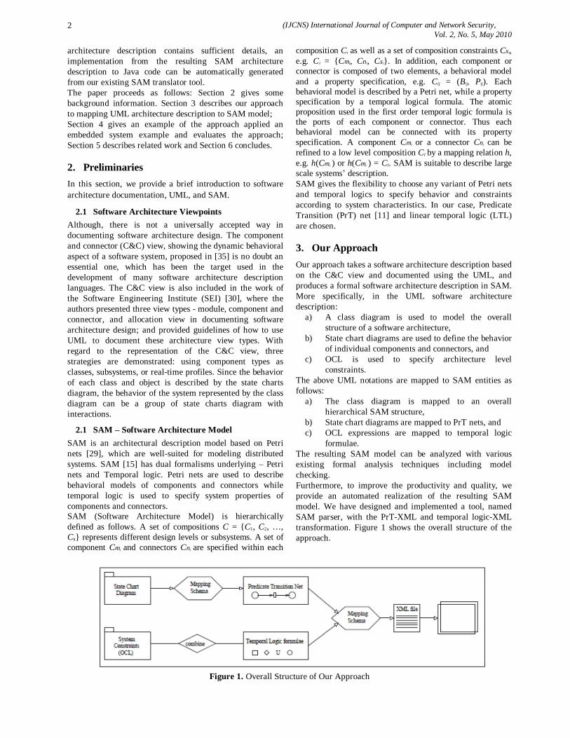
3. Our Approach Our approach takes a software architecture description based on the C&C view and documented using the UML, and produces a formal software architecture description in SAM. More specifically, in the UML software architecture description:
a) A class diagram is used to model the overall structure of a software architecture,
b) State chart diagrams are used to define the behavior of individual components and connectors, and
c) OCL is used to specify architecture level constraints.
The above UML notations are mapped to SAM entities as follows:
a) The class diagram is mapped to an overall hierarchical SAM structure,
b) State chart diagrams are mapped to PrT nets, and c) OCL expressions are mapped to temporal logic
formulae. The resulting SAM model can be analyzed with various existing formal analysis techniques including model checking. Furthermore, to improve the productivity and quality, we provide an automated realization of the resulting SAM model. We have designed and implemented a tool, named SAM parser, with the PrT-XML and temporal logic-XML transformation. Figure 1 shows the overall structure of the approach.
Figure 1. Overall Structure of Our Approach
(IJCNS) International Journal of Computer and Network Security, Vol. 2, No. 5, May 2010
3
3.1 Mapping from State-charts to SAM Composition
It is straightforward to map each class into a composition in a SAM model. In this section, we mainly focus on the mapping from state charts to a SAM composition. A statechart diagram specified the states that an object can inhabit in, describes the events triggered flow of control and actions responded from the system, as the result of the objects reactions to events from the environment. The semantics of statecharts is based on the run-to-completion assumption [1]. A State is an abstract metaclass that models a situation during which some (usually implicit) invariant conditions hold. The structure of a state vertex, defined by the following function children, incarnates the hierarchy of state machines. Definition 1 (Children). Let S be a set of state vertices. The function children: S defines for each state the set of its direct substates. We define childreni(s) = s’|s’ ∈ childreni-1(s) for i > 1. Thus the function children+(s) = ∪i>0childreni(s) defines for each state a set of its transitively nested substates. Incoming events are processed one at a time and an event can only be processed if the processing of the previous event has been completed – when the statechart component is in a stable state configuration. In our study, we considered the events and actions defined by the methods which are specified in the corresponding classes. Thus we can obtain more detailed implementation information. To map the state chart diagram to SAM composition, we present a translation algorithm (fT) in the following steps.
a) Each super state S, where children(S) ≠ Φ, is mapped into a composition C in SAM model, i.e., fT(S) = Ci, where children(S) ≠ Φ.
b) Each substate s ∈ S, where children(S) = Φ, is mapped into a component Cm ∈ C. We have fT(S) = Cm, where children(S) = Φ, Cm ∈ C, and Cm = < Bm, Pm> . Let S be < En,Ex,Do,A,G> , where En, Ex, Do, and A represent entry, exit, do and other regular actions taken inside the states respectively, G denotes the guard of any actions.
b.1 The behavior model of the component (Bm) is described by following mapping: fT(S) = <<pt_in, ten>, <pt_out, tex>, ti, gt >, where pt_in, and pt_out denote input and output port respectively, ten and tex denotes transitions that are corresponding to entry and exit action respectively, ti denotes transitions that corresponding to the do action and other internal actions, gt denotes the internal transition’s guard function.
b.2 The property specified (Pm) by OCL can be transformed into first order (or propositional) logic and temporal logic.
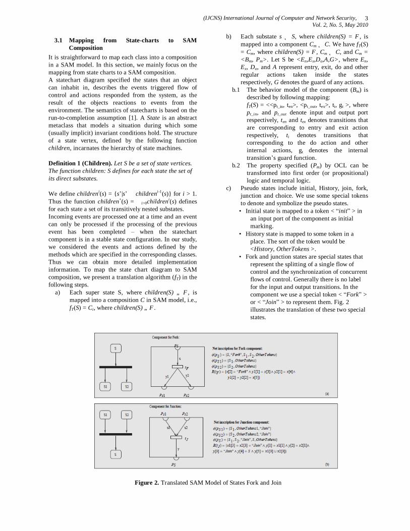
c) Pseudo states include initial, History, join, fork, junction and choice. We use some special tokens to denote and symbolize the pseudo states.
• Initial state is mapped to a token < “init” > in an input port of the component as initial marking.
• History state is mapped to some token in a place. The sort of the token would be <History, OtherTokens >.
• Fork and junction states are special states that represent the splitting of a single flow of control and the synchronization of concurrent flows of control. Generally there is no label for the input and output transitions. In the component we use a special token < “Fork” > or < “Join” > to represent them. Fig. 2 illustrates the translation of these two special states.
Figure 2. Translated SAM Model of States Fork and Join
(IJCNS) International Journal of Computer and Network Security, Vol. 2, No. 5, May 2010
4
d) A transition tS inside the super state S is mapped
into a connector Cn ∈ C. Let S be <E,A,Valr,G> . In this case, we have: fT (< E,A,Valr,G>) = <<pt_in, t>, <pt_out, t>, tk, gt_internal>, where E denotes trigger event or action, A denotes action, pt_in, and pt_out denote input and output port respectively, t denotes transition, tk denotes tokens in the ports, Valr denotes returned value of the action A, and G denotes guard of the label, gt_internal denotes the internal transition’s guard function.
e) Generally, we can merge the place holding the return value for entry action with the place holding the parameters for the do action, the holding the return value for do action with the place holding the parameters for the exit action.
From above translation algorithm (fT), we can realize a mapping relation between each item in the state-chart diagram and the SAM architecture model. This translation algorithm (fT) is meaningful for the formal verification of UML architecture document.
3.2 Mapping from OCL to First Order Temporal Logic
In the translation from OCL to first order and temporal logic, it is worth to note that following features of OCL restrict the translation to temporal logic.
1. There is not timing concept in the OCL specification.
2. There is not object concept in the temporal logic specification.
3. OCL is an implementation-based and oriented specification language, while temporal logic is a high level specification language. Thus there is not type system, data structure, condition and flow control sentence in temporal logic.
4. Finally, OCL is 3-value function logic (true, false, and undefined,) while temporal logic is a 2-value logic.
Considering the above features and difference between OCL and temporal logic and first order logic, we decide to map OCL expression to the first order logic with the following concerns:
• Context: It indicates the scope of the entity. It can be translated to the quantifiers ∀ or ∃. The difference is that the scope of the quantifiers in the OCL context generally is finite.
• Navigation: Navigation through association either results in a Set(Object) or in a Seq(Object) if association is marked as ordered. We can use a quantifier ∃ on Set(Object), Seq(Object) or Collection, since the later two also have the set concept. In addition, select and reject used in the Collection can be mapped to the quantifiers ∀ and ∃, since they restrict the scope of instances.
• forall and exists: are obviously translated into quantifiers ∀ and ∃.
• allinstance: It semantically matches ∃. • operations, attributes: All predefined boolean
operations can be mapped into first order logic operations. All mathematic operations can be used
directly. Some other predefined operations, such as toUpper(), Concat() have no images in the logic domain. Attributes can be (atomic) predicates in the first order or propositional logic.
• invariants: This means that the constraints are always holding in the context, thus it is a context-specific safety property: invariants
• pre- and post-condition: can be mapped to the following temporal formula precondition → ⋄ postcondition. In the case that it is an invariants, we have (precondition → ⋄postcondition)
• let-in clause: let clause defines some variables used in the in clause. In the in clause, you can use any defined syntax in the OCL.
• if-then-else clause: Let use format if cond then r1 else r2, we have the logic formula as follows
cond → r1 ∨ r2. • previous value @pre: The postfix @pre refers to a
value of a property at the start of an operation in a postcondition. In this case we have to record the previous value and then invoke the value through some method since there is not a corresponding mapping in the logic.
3.3 Tool Support – SAM Translator Runtime verification, composed of a software module and an observer, monitors the execution of a program, and checks its conformity with a requirement specification, often written in a temporal logic. Runtime verification can be applied to evaluate automatically test runs, either on-line or o_-line, analyzing stored execution traces; or it can be used on-line during operation, potentially steering the application back to a safety region if a property is violated. It is highly scalable. Several runtime verification systems have been developed, such as JPaX [14], Java-MAC [17], etc.. We have developed a runtime monitoring system, SAM Parser, on Software Architecture Model (SAM) [15] whose behavior is modeled by Petri Nets and properties by temporal logic. To validate the translated state charts model, we adapted it to SAM parser to reuse that tool. We introduce the SAM Parser simply introduced in the following. Input: The runtime checker has to have two input data: transformed SAM model and temporal logic. These data are specified in the PNML and XML format. Code Generation: The code of SAM model and temporal logic and first order logic formulae are automatically generated from the input files. In our work, we construct a class as a child of templates for each net, place, transition, arc, inscription, initial marking, and guard. The reason for this is to make it easier to understand and maintain. For example, the user can provide a more efficient way to check the enableness of a transition and the way to fire it by replacing methods of corresponding classes without any side effects on other transitions. The execution of generated code is non-deterministic, i.e. we choose an enabled transition and a valid assignment randomly to fire. It is hard to generate code automatically given a Petri net due to the complexity of sorts, guard conditions of transition and arc labels [25]. If some restrictions[10] are satisfied, we can achieve it.
(IJCNS) International Journal of Computer and Network Security, Vol. 2, No. 5, May 2010
5
Temporal logic and first order logic formulae are transformed into automata by a logic engine Maude ([5]). These translated automata will feed into our runtime checker generator to produce monitors for different formulae. Runtime Checker Generation: Runtime checkers are generated by breaking the temporal logic formula into subformulae and creating a matrix for the formula [33]. In order to generate monitoring codes for properties (linear temporal formulae), a logic server, Maude [5] in our case, is necessary. Maude, acting as the main algorithm generator in the framework, constructs an e_cient dynamic programming algorithm (i.e. monitoring code) from any LTL formula [33]. The generated algorithm can check if the corresponding LTL formula is satisfied over an event trace.
4. An Application of the MDA Approach We present an instance of our approach in a statechart diagram, which is one of the state machine in the UML models, through a case study. The case study deals with a simplified cruise control system adapted from [13]. In this section we will first introduce the cruise control system and a state chart diagram for the cruise controller. Then we present some properties of this example. Finally, the runtime verification results are discussed.
4.1 Cruise Control System and UML Documentation The purpose of a cruise control system is to accurately maintain the driver’s desired set speed, without
intervention from the driver, by actuating the throttle-accelerator pedal linkage. A modern automotive cruise control is a control loop that takes over control of the throttle, which is normally controlled by the driver with the gas pedal, and holds the vehicle speed at a set value. We assume an automatic transmission vehicle. When turned on by the driver, a cruise-control system (CCS) automatically maintains the speed of a car over varying terrain. The CCS can be turned on by pressing Start button, and enabled by pressing SetSpeed button. Resume button will enable the CCS at the last maintained speed when the brake is released. The cruise control function is disabled when the brake or accelerator pedal is pressed. Pressed once Resume button can increase the speed with 1mph and the SetSpeed button can decrease the speed with 1mph when the cruise control function is enabled. The cruise control system should be automatically disabled when the speed is below 25mph and above 90mph. For the space limit, we cannot show the UML diagram and generated code. Each place or port must carry its state information which is also ignored in the tables. Finally, we have to point out that the guard function for a transition has to be added some more restrictions for the evaluations. For instance, if there is a token “void” in the input place of a transition, it means the previous action does not have return value, we have to justify that field to evaluate the firing condition of the transition. This means that automatically mapping a guard condition in a state chart diagram to a guard function is not sufficient in some cases.
4.2 Experiment Results and Discussion The time of generated code with monitors is 4.3s. We checked 5 properties covering 5 components and 4 connectors. Since the events and actions are defined by the methods which are specified in the corresponding classes, each fired transition represents a method is operated under some guard condition. The properties specified in the OCL expressions for the state chart diagram is mapped to temporal formulae and further used to generate monitors.
All properties are true if the conditions and guard are satisfied. We also check some conditions that is not suitable for the method, such as different parameters feeding for the method that makes the guard is not satisfied, in that case the formula is evaluated as false. The Results are consistent with what we expected from the state chart diagram. Finally, we also find a mapping mistake in the component Accelerating and component Decelerating when we check properties relative to them. We modified the mapped SAM composition according to the checking results.
5. Related Work Our MDA approach and the presented framework integrate two aspects: software architecture with UML design notation and its extension. Moreover, our approach also provided a runtime validation and verification technique by using SAM Parser. The related works are discussed in the following. Formal Modeling and Analysis of Architecture Descriptions in UML: Our work has been influenced by a large body of research and practical experience. In the interest of brevity, we only compare it to the most relevant approaches. The work reported in this paper relates to works that focus on specifying structural and possibly behavioral aspects of a software system using UML. The representative UML architecture description examples are provided by Kruchten [21], Hofmeister et al. [16] and Clements et al. [31]. Although several researchers have explored the formal
analysis of generic UML object-oriented designs [7, 34, 12, 24, 4, 26, 35], their results may not be ready applicable to UML architecture level designs. Code Generation from the UML Description and Verification in the Implementation: There is a significant amount of research that considers mappings from UML to other (mostly formal) modeling techniques to validate UML models (e.g. using B [22], CSP [8], SPIN [23], PVS [2], Petri Nets [27, 38], Z/Eves [3] and the work with Object-Z [19, 20, 18, 39]). These works focus on the mapping from UML diagrams to formal methods for model checking or some specification language for the model checkers. Moreover, less of them address the code generation and verification in the implementation level. Property Specification – OCL Expression and Temporal Logic: Various methodologies proposed to deal with the property specification of object-oriented systems. There are two main streams to cooperate OCL with temporal logics, one is extending OCL with temporal notations ([31, 9, 37]
(IJCNS) International Journal of Computer and Network Security, Vol. 2, No. 5, May 2010
6
etc.), another is add object concepts into temporal logics ([6]). The work in both streams increases the complexity of the extended language and obstacles of the usage.
6. Conclusion and Future Works In this paper, we have presented an integrated approach for transferring an architecture description represented in UML to a formal architecture model represented in SAM, which not only supports design level analysis but also automated code generation with run-time verification capability. The specific details of the approach, outlined in the algorithms in Section 3, are likely to evolve as our research on the relationship between UML and software architectures deepens; however, we believe that the approach is flexible and general enough to accommodate needed new changes. As pointed out by Medvidovic in the work [27] ensuring system properties at the level of architecture is of little value unless it can also be ensured that those properties will be preserved in the resulting implementation. This reflects the importance of the code generation and runtime verification of system properties in the implementation. Our automated code generation and run-time verification approach nicely addresses the above research issue. Acknowledgements We appreciate for all reviewers to read this paper. This work is supported by Title III under grant PO31B085057-08.
References [1] Uml 2.0 specification. http://www.omg.org/
technology/documents/formal/uml.htm. [2] Enhancing Structured Review with Model-Based
Verification. IEEE Transaction on Software Engineering, 30(11):736–753, 2004. Member-Issa Traore and Member-Demissie B. Aredo.
[3] N. Am´alio, S. Stepney, and F. Polack. Formal proof from uml models. In ICFEM’04, volume 3308 of Lecture Notes in Computer Science, pages 418–433, 2004.
[4] D. B. Aredo. Semantics of UML statecharts in PVS. In Proceeding of 12th Nordic Workshop on Programming Theory, Bergen, Norway, 2000.
[5] M. Clavel, F. J. Dur´an, S. Eker, P. Lincoln, N. Mart ı-Oliet, J. Meseguer, and J. F. Quesada. Maude: Specification and Programming in Rewriting Logic. http://maude.csl.sri.com/papers, March 1999.
[6] D. Distefano, J.-P. Katoen, and A. Rensink. On a Temporal Logic for Object-Based Systems. In S. F. Smith and C. L. Talcott, editors, Formal Methods for Open Object-Based Distributed Systems IV - Proc. FMOODS’2000, Stanford, California, USA, September 2000. Kluwer Academic Publishers.
[7] Z. Dong and X. He. Integrating UML State-chart and Collaboration Diagrams Using Hierarchical Predicate Transition Nets. In GI Lecture Notes in Informatics, 2001.
[8] G. Engels, R. Heckel, and J. M. K¨uster. Rule-based specification of behavioral consistency based on the UML meta-model. volume 2185, pages 272–284, 2001.
[9] S. Flake and W. Mueller. An OCL extension for real-time constraints. In Object Modeling with the OCL, pages 150–171, 2002.
[10] Y. Fu, Z. Dong, and X. He. A Methodology of Automated Realization of a Software Architecture Design. In Proceedings of The Seventeenth International Conference on Software Engineering and Knowledge Engineering (SEKE2005), 2005.
[11] H. J. Genrich. Predicate/Transition Nets. Lecture Notes in Computer Science, 254, 1987.
[12] M. Gogolla and F. P. Presicce. State Diagrams in UML: A Formal Semantics using Graph Transformations. In Proceedings of International Conference of Software Engineering, Workshop on Precise Semantics of Modeling Techniques, pages 55–72, 1998.
[13] H. Gomaa. Designing Concurrent, Distributed, and Real-Time Applications with UML. Addison-Wesley Professional, 2000.
[14] K. Havelund and G. Rosu. An overview of the runtime verification tool java pathexplorer. Journal of Formal Methods in System Design, 2004.
[15] X. He and Y. Deng. A Framework for Specifying and Verifying Software Architecture Specifications in SAM. volume 45 of The Computer Journal, pages 111–128, 2002.
[16] C. Hofmeister, R. L. Nord, and D. Soni. Describing Software Architecture with UML. In Proceedings of the TC2 1st Working IFIP Conference on Software Architecture (WICSA1), pages 145 – 160, 1999.
[17] M. Kim, S. Kannan, I. Lee, and O. Sokolsky. Java-MaC: a Run-time Assurance Tool for Java. In Proceedings of RV’01: First International Workshop on Runtime Verification, Paris, France, Electronic Notes in Theoretical Computer Science. Elsevier Science, 2001.
[18] S.-K. Kim, D. Burger, and D. Carrington. An mda approach towards integrating formal and informal modeling languages. In FM 2005: Formal Methods, International Symposium of Formal Methods Europe,, volume 3582 of Lecture Notes in Computer Science, pages 448–464, 2005.
[19] S.-K. Kim and D. Carrington. Formalizing the UML Class Diagrams Using Object-Z. In UML’99: The Unified Modeling Language - Beyond the Standard, Second International Conference, volume 1723 of Lecture Notes in Computer Science, 1999.
[20] S.-K. Kim and D. Carrington. A Formal Mapping between UML Models and Object-Z Specifications. Lecture Notes in Computer Science, volume 1878, pages 2–21, 2000.
[21] P. Kruchten. The 4+1 view model of architecture. IEEE Software, 12(6):42–50, 1995.
[22] K. Lano, D. Clark, and K. Androutsopoulos. UML to B: Formal Verification of Object-Oriented Models. volume 2999 of Lecture Notes in Computer Science, pages 187–206,2004.
[23] D. Latella, I. Majzik, and M. Massink. Automatic Verification of a Behavioural Subset of UML Statechart Diagrams Using the SPIN Model-checker. Formal Aspects of Computing, 11(6):637 – 664, 1999.

(IJCNS) International Journal of Computer and Network Security, Vol. 2, No. 5, May 2010
7
[24] D. Latella, I. Majzik, and M. Massink. Towards a Formal Operational Semantics of UML Statechart Diagrams. In Proceedings of the 3rd IFIP International Conference on Formal Methods for Open Object-based Distributed Systems, pages 331–347, February 1999.
[25] S. W. Lewandowski and X. He. Generating Code for Hierarchical Predicate Transition Net Based Designs. In Proceedings of the 12th International Conference on Software Engineering & Knowledge Engineering, pages 15–22, Chicago, U.S.A., July 2000.
[26] J. Lilius and I. P. Paltor. The Semantics of UML State Machines. Technical Report 273, Turku Centre for Computer Science, 1999.
[27] N. Medvidovic, D. S. Rosenblum, and D. F. Redmiles. Modeling Software Architectures in the Unified Modeling Language. ACM Transactions on Software Engineering and Methodology, 11(1):2–57, January 2002.
[28] H. Motameni. Mapping to Convert Activity Diagram in Fuzzy UML to Fuzzy Petri Net. World Applied Sciences Journal, 3(3): 514 – 521, 2008. ISBN: 1818-4952.
[29] T. Murata. Petri Nets: Properties, Analysis and Applications. Proceedings of the IEEE, 77(4):541–580, 1989.
[30] J. S. e. a. Paul Clements, Len Bass. Documenting Software Architectures: Views and Beyond. Addison-Wesley, January 2003.
[31] S. Ramakrishnan and J. McGregor. Extending OCL to Support Temporal Operators. In 21st International Conference on Software Engineering (ICSE 99), Workshop on Testing Distributed Component-Based Systems, May 1999.
[32] J. E. Robbins, N. Medvidovic, D. F. Redmiles, and D. S. Rosenblum. Integrating architecture description languages with a standard design method. In ICSE ’98: Proceedings of the 20th international conference on Software engineering, pages 209–218, Washington, DC, USA, 1998. IEEE Computer Society.
[33] G. Rosu and K. Havelund. Rewriting-Based Techniques for Runtime Verification. Journal of Automated Software Engineering, 2004.
[34] J. Saldhana and S. M. Shatz. UML Diagrams to Object Petri Net Models: An Approach for Modeling and Analysis. In Proceedings of the International Conference on Software Engineering and Knowledge Engineering, pages 103–110, 2000.
[35] T. Sch¨afer, A. Knapp, and S. Merz. Model Checking UML State Machines and Collaborations. Electronic Notes in Theoretical Computer Science, 55(3):1–13, 2001.
[36] M. Shaw and D. Garlan. Software Architecture: Perspectives on an Emerging Discipline. Prentice Hall, 1996.
[37] P. Ziemann and M. Gogolla. An Extension of OCL with Temporal Logic. In Critical Systems Development with UML – Proceedings of the UML’02 workshop, pages 53–62, TUM, Institut fur Informatik, TUM-I0208, September 2002.
[38] Jiexin Lian, Zhaoxia Hu, Sol M. Shatz. Simulation-based analysis of UML statechart diagrams: methods and case studies. Software Quality Journal. 16(1), March, 2008. ISBN: 0963-9314. Springer Netherlands.
[39] Rafael M. Borges and Alexandre C. Mota. Integrating UML and Formal Methods. Electronic Notes in Theoretical Computer Science (ENTCS). Volume 184. Page 97-112. July 2007. Elsevier Science Publishers.
Authors Profile Yujian Fu received the B.S. and M.S. degrees in Electrical Engineering from Tianjin Normal University and Nankai University in 1992 and 1997, respectively. In 2007, she received her Ph.D. degree in computer science from Florida International University. She joined the faculty of Department of Computer Science at the Alabama A&M University in the same year. Dr. Yujian Fu conducts research in the software verification, software quality assurance, runtime verification, and formal methods. Dr. Yujian Fu also actively serves as reviewers of several top journals and prestigious conferences. She continuously committed as a member of IEEE, ACM and ASEE. Zhijiang Dong received the B.S. and M.S. degrees in Huazhong Tech University, Ph.D. degree in computer science from Florida International University. He currently is assistant professor at Middle Tennessee University. Dr. Dong’s research is mainly in the software engineering. Dr. Dong also actively serves as reviewers of several top journals and conferences. He continuously committed as a member of IEEE, ACM. Xudong He is a professor of school of computing and information science and director of center for advanced and distributed system engineering at Florida International University. Dr. He’s research are software engineering, formal verification and specification. Dr. He currently has over one hundred publications in prestigious journals and conferences. Sha Li is an associate professor at department of curriculum, teaching and educational leadership, school of education of Alabama A&M University. Dr. Sha Li received his doctorial degree of educational technology from Oklahoma State University, 2001. Sha Li' research interests include distance education, instructional technology, instructional design and multimedia for learning. Phil Bording is an associate professor and chair of department of computer science at Alabama A&M University. Dr. Phil Bording received his Ph.D. degree in computer science from University of Tulsa in 1995 and M.S. degree from University of Alabama at Huntsville in 1984. Dr. Bording’s research area is parallel computing.
(IJCNS) International Journal of Computer and Network Security, Vol. 2, No. 5, May 2010
8
Principle Component Analysis From Multiple Data Representation
Rakesh Kumar yadav1, Abhishek K Mishra 2, Navin Prakash3 and Himanshu Sharma4
1College of Engineering and Technology, IFTM Campus,
Lodhipur Rajput, Moradabad, UP, INDIA [email protected]
2College of Engineering and Technology, IFTM Campus,
Lodhipur Rajput, Moradabad, UP, INDIA [email protected]
3College of Engineering and Technology, IFTM Campus,
Lodhipur Rajput, Moradabad, UP, INDIA [email protected]
4College of Engineering and Technology, IFTM Campus,
Lodhipur Rajput, Moradabad, UP, INDIA [email protected]
Abstract: For improving accuracy and increasing efficiency of classifier, there are available many effective techniques. One of them combining multiple classifier technique is used for this purpose. In this paper I present a novel approach to a combining algorithm designed to improve the accuracy of principle component classifier. This novel approach combines multiple PCA classifiers, each of using a subset of feature. In contrast other combining algorithms usually manipulate the training pattern. Keywords: PCA classifier, Eigenface, Eigenvector, Voting, Covariance matrix, new projected data, face recognition.
1. Introduction The PCA classifier is one of the oldest and simplest methods for classification. PCA involves a mathematical course of action that transform a number of possible correlated variable into a smaller no of uncorrelated variable called principle component. PCA is mathematically defined as an orthogonal linear transform that transform the data to a new coordinate system such that greatest variance by any projection of the statistics comes to lie on the first coordinate. The second greatest variance on the second coordinate and so on [10]. 1.1. Method of Pronouncement PCA. Step 1: Acquire some data Step 2: Subtract the mean Step 3: Compute the covariance matrix Step4: Compute the eigenvectors and eigenvalues of the covariance Matrix Step 5: Choosing components and forming a feature vector Step 6: Deriving the new data set. 1.2. Related work Image classification is a thorny task because images are multidimensional. There are many classifiers although there are a number of face recognition algorithms which works well in constrained situation; face recognition is still an
open and very challenging dilemma in real application. The area of face recognition has focused on detecting individual feature such as the eyes, nose, mouth, lips and head outline and defining face model by the position, size, perimeter and relationship among features. Bledsoe’s [3] and Kanade’s [4] recognition based on these parameter. A Mathew A. Turk and Alex P. Pentland [1] track a subject’s and then recognizes the person by comparing characteristics of the face to those of known individuals. Face images are projected onto a feature space that best encodes the variation among known face images. The face space is defined by the “eigenface” which are the eigenvectors of the set of faces; they do not necessarily correspond to isolated feature such as eyes, ear and nose. The framework provides the ability to learn to recognize new faces in an unsupervised manner. In mathematical terms, we want to find the principle component of the distribution of faces or the eigenvectors of the covariance matrix of set of face images. These eigenvectors can be thought of as a set of feature which together characterizes the variation between face images. Each image location contributes more or less to each eigenvector so that we can display the eigenvector as a sort of ghostly face which we call an eigenfaces. There are many approaches available to combining the classifier such as Stephen O.Bay, “Nearest Neighbor Classification from Multiple Feature Subset” [7] and Bing-Yu-Sun- Xiao-Ming Zhang and Rujing Wans, “Training SVMs for Multiple Feature Classifier Problem” [5] but there in no any approach available to combining the base classifiers. Actually the combination of classifier can be implemented at two levels, feature level and decision level. Xiaoguang Lu, Yunhong Wang, Anil K. Jain, “combining classifier for face recognition”[4] provide frameworks to combine different Classifier on feature based .We are using feature level combination and want to present combination of classifier which works on low level feature in this approach.

(IJCNS) International Journal of Computer and Network Security, Vol. 2, No. 5, May 2010
9
2. Classification amalgamation 2.1. Training Phase In the training phase we extract feature vector for each subset of images in training data set. Let T1 be a training subset in which every image has pixel resolution of M by N (M row, N column). In order to extract PCA features of T1 we will first convert image into a pixel vector by concatenating each of M rows into single vector V1. The length of pixel vector V1 will be M*N. we will use the PCA algorithm as a dimensionality reduction technique which transform the vector V1 to a vector W1. Which has dimensionality d where d<=M*N. For each training image subset Ti, we will calculate and store these feature vector Wi. 2.2 Recognition Phase In the recognition phase, we will be given a test set of images Tj of known person. As in the training phase we will compute the feature vector of this test set using PCA and match the identity name of persons. In order to identity we will compute the similarities between test set and training subset. For this we will use the combining algorithm method. 2.3. Combining algorithm. The algorithm for PCA classification from multiple feature subsets is simple and can be treated as: Using voting, combining the output from multiple PCA classifiers each having access each subset of feature. We select the subset of features by sampling from original set of features we use two different sampling functions: sampling with replacement and sampling without replacement. In sampling with replacement a feature can be selected more than once which we treat as increasing its weight. Each of the PCA classifiers uses the same number of features. This is parameter of algorithm which we set by cross confirmation performance estimates on the training set. The similarity among new projected data can be calculated using euclidean distance the identity of most similar Wi will be output of our classifier. If i=j it means that we have correctly identified the subset otherwise we have misclassified the subset. The schematic diagram of this presented in figure 1. 2.4. Pseudo code of combining algorithm
1. Prepare training set which contains subset of images
2. Set PCA dimensionality parameter 3. Read training subset 4. Form training data matrix. 5. Form training class label matrix 6. Calculate PCA transform Matrix 7. Calculate feature vector , projected data of all
subset of training set by using PCA transformation matrix
8. Store training feature vector and projected data in a matrix.
9. Read test set
Figure 1
10. Calculate the feature vector of test set and also
calculate new projected data buy using PCA transformation matrix.
11. Compute the similarity between subset and test set by using voting method.
12. store the similarity 13. Now we go the subset test set which have lowest
similarity factors determine the person id and match the id between training subset and test set.
14. Initialize error count to zero 15. For each test face If the id is match then
recognition done and accuracy will be hundred percent.
16. If the id of any test face image is not equal to id of training subset of each image then increment in error count.
17. Compute the accuracy by using error count value.
3. Experiment Discussion To access the possibility of this approach to face recognition, we have performed experiments .we used the ORL database [9] which available in public domain. We also used image processing tool of MATLAB 7.6. Using ORL database we have conducted 3 experiments to access the accuracy of recognition by formula: (1-(error count/total test image count))*100 In the experiments we take 5 training subset of face image. Each subset contains 20 face images of 4 different person and one test set which contains 5 images of a person. In the first experiment we set up 60 percent accuracy. In the
(IJCNS) International Journal of Computer and Network Security, Vol. 2, No. 5, May 2010
10
second experiment we set up 80 percent accuracy and at last in third experiment we found 60 % accuracy. As can seen my result are no where near perfect yet with my best outcomes in with almost 80 percent matches. If we study this approach in the view of complexity then definitely I assured both time and space complexity will be reduced because we are using multiple feature subset concepts as like in nearest neighbor classifier from multiple feature subsets [7]. The nearest neighbor classifier from multiple feature subsets supports lower complexity.
4. Conclusion and future work As can be seen my results are near to perfect while these results may be improve. Conceptually this approach reduced the complexity also but this approach has two limitations one voting can only improve accuracy if the classifier select the correct class more often than only other class. Another algorithm has two parameter value need to be set first is size of features subset and second is number of classifier. So in the near future we can also improve the accuracy and complexity of this approach.
5. References [1] M. Turk and A. Pentland,”Face recognition using
eigenface”, In Computer Vision and Pattern Recognition, 1991.
[2] W.W.Bledsoe, “the model method in facial recognition”, panoramic research inc. Palo alto.ca roe. Pr: 15, Aug 1966
[3] T. Kanade, “picture processing system by computer complex and recognition of human faces”, dept pf information science, Kyoto university, Nov 1973.
[4] Xiaoguang Lu, Yunhong Wang, Anil K. Jain, “combining classifier for face recognition”.
[5] Bing-Yu-Sun- Xiao-Ming Zhang and Ru-jing Wang, “Training SVMs for Multiple feature classifier problem”.
[6] Julein Meynet Vlad Popovici, Matteo, Sorci and jean Philippe Thiran, “combining SVMs for face class modeling”.
[7] Stephen D.Bay,” Nearest neighbor classification from multiple feature subset”, November 15, 1998.
[8] Linday I smith, “A tutorial on principle component analysis”, February 26, 2002
[9] http://homepages.cae.wiseedu/~ece533/ [10]http://en.wikipedia.org/wiki/Principal_component_anal
ysis Authors Profile Rakesh Kumar Yadav received the B.Tech Degree in Information Technology from A K G Engineering College Ghaziabad, INDIA in 2004. Currently pursuing M.Tech and Working as Sr. Lecturer in college of Engineering and Technology, IFTM Moradabad. INDIA.
Abhishek K Mishra received the M.Tech Degree in computer Technology and Application from school of Information Technology, UTD, RGPV, Bhopal, India.. Currently Working as Sr. lecturer in college of Engineering and Technology, IFTM Moradabad. INDIA. Navin prakash received the B Tech Degree in Computer Science from BIET Jhansi in 2001, India. Currently Working as Sr. lecturer in college of Engineering and Technology, IFTM Moradabad. INDIA. Himanshu Sharma received the B.Tech Degree in computer Science and Information technology from MIT, Moradabad, India. Currently Working as Sr. lecturer in college of Engineering and Technology, IFTM Moradabad, INDIA.

(IJCNS) International Journal of Computer and Network Security, Vol. 2, No. 5, May 2010
11
Performance Evaluation of MPEG-4 Video Transmission over IEEE802.11e
Abdirisaq Mohammed Jama1, Sinzobakwira Issa2 and Othman O. Khalifa3
1International Islamic University Malaysia,
Department of Electrical & Computer Engineering, P.O.Box 10, 50728, Kuala Lumpur, Malaysia
2International Islamic University Malaysia, Department of Electrical & Computer Engineering,
P.O.Box 10, 50728, Kuala Lumpur, Malaysia [email protected]
3International Islamic University Malaysia,
Department of Electrical & Computer Engineering, P.O.Box 10, 50728, Kuala Lumpur, Malaysia
Abstract: Transmitting MPEG-4 video over Wireless Local Area Networks is expected to be an important component of many emerging multimedia applications. One of the critical issues for multimedia applications is to ensure that the Quality of Service (QoS) requirement to be maintained at an acceptable level. The IEEE802.11 working group developed a standard called IEEE802.11e to support Quality of Service (QoS) in WLANs. This standard aims to support QoS by providing differentiated classes of service at the Medium Access Control (MAC) layer to enhance the ability of physical layers to deliver time-critical traffic in the presence of traditional data packets. In this Paper, Network Simulator 2 (NS-2) & Evalvid are used as simulation tool to evaluate the Performance of MPEG-4 Video Transmissions over IEEE802.11e. A modification of the parameters of NS-2 and Evalvid were done to present the evaluated method. This has allowed us to control the different design metrics values such as Frame/Packet loss, PSNR & Decodable Frame Rate (Q). In this paper, we evaluate a framework which consists of a MAC-centric cross-layer architecture to allow MAC layer to retrieve video streaming packet information, and a single-video multi-level queue to prioritize I/P/B slice (packet) delivery, the evaluated systematic scheme shows better results for lower packet loss, higher PSNR & Decodable Frame Rate (Q) for MPEG-4 video transmission over IEEE 802.11e..
Keywords: IEEE802.11e, MPEG-4, NS-2, Evalvid.
1. Introduction Efficient video transmission over wireless remains one of the challenging goals for multimedia communications because of the scarce wireless resources, high bandwidth and quality of service (QoS) requirement for video transmission. However, studies on the MPEG-4 video transmission in the wireless networks are not well explored. This paper proposes a study of the transfer of video sequences coded in MPEG-4 over wireless networks using the IEEE802.11e technology. Quantifying the effects of these simulations will help us in the design of a scheme for
the adaptation of MPEG-4 Video transmission over wireless channel. In the following section 2, we briefly preview the related work involved in the transmission of MPEG-4 video packets over IEEE802.11e. Section 3 presents the simulation set-up, & Network topology of our simulation study. In section 4, simulation results are presented and discussed. The conclusion is given in Section 5 followed by the References.
2. Related Work IEEE802.11 is one of most popular medium access control protocols in the world. However, with IEEE802.11 it is difficult to guarantee QoS because all stations use the equal access method and network parameters. With the development of services such as multimedia streaming, the demands for QoS guarantees are increasing. The IEEE standard [13] proposed IEEE802.11e medium access control protocol for QoS guarantee extends the existent and enhancements of IEEE802.11 Medium Access Control protocols and newly defines the HCF (Hybrid Coordination Function). HCF proposed two methods: EDCA (Enhanced Distributed Channel Access) and HCCA (HCF Controlled Channel Access). The EDCA model is the competition base medium access method and the HCCA model is a polling base medium access method to act under the control of the HC (Hybrid Coordinator). The EDCA model is designed to provide a differentiation service based on priority, and is similar with the DCF (Distributed Coordination Function) model of existing 802.11 MAC. The EDCA model is the defining concept of AC (Access Category) for QoS support. Each AC has competition parameters, AIFS [AC] (Arbitration Inter-frame Space) that alternate DIFS (Distributed Inter-frame Space), CWmin [AC] and CWmax [AC] [1], [2].

(IJCNS) International Journal of Computer and Network Security, Vol. 2, No. 5, May 2010
12
Fig. 1 shows the structure of IEEE802.11e EDCA model, Wireless Station (WSTA) that have QoS parameters to decide priority and four transmission queues that are recognized by the virtual station. If more than two values of the back-off counter in a station reach to 0 at the same time, the scheduler of WSTA prevents a virtual collision.
Figure 1. Structure of IEEE802.11e model
Fig. 2 shows the medium access method of the EDCA model. Each frame has an AIFS [AC] of different size according to the priority. Frames of highest priority have IFS (Inter-frame Space) such as DIFS, and low priority frames have longer IFS than others. As a result, the probability of access to the medium of frame and the priority of frame are in proportion. The sizes of the competition windows are different CWmin [AC] and CWmax [AC] according to each AC.
Figure 2. Medium Access Control method of IEEE802.11e EDCA
If the priority of the frame is high, it has a small CWmin [AC] and CWmax [AC]. Therefore, the latency times to medium access of the high priority frames can be reduced even if a collision arises, and the data in transmission queue can have a transmission opportunity easily.
There is much research taking place on transmitting multimedia video efficiently using the medium access control method of the IEEE802.11e EDCA model [3],[4],[5]. Techniques, among the ones being researched to improve quality of service, use the discriminating medium access control method of IEEE802.11e EDCA model according to the importance of the video data type [6].
However, these techniques can create attempts at unnecessary data transmission that exceed available bandwidth of networks because it does not have an adaptive transmission rate adjustments scheme. As a result, transmission queue overflow or loss of data causes degradation in the quality of the video streaming service. In [7] the authors classify cross-layer architectures for video transport over wireless networks into five categories:- 1. Top-down approach: the higher-layer protocols optimize their parameters and the strategies at the next lower layer. 2. Bottom-up approach: the lower layers try to insulate the higher layers from losses and bandwidth variations. 3. Application-centric approach: the APP layer optimizes the lower layer parameters one at a time in a bottom-up (starting from the PHY) or top-down manner, based on its requirements. 4. MAC-centric approach: the APP layer passes its traffic information and requirements to the MAC, which decides which APP layer packets/flows should be transmitted and at what QoS level. 5. Integrated approach: strategies are determined jointly by all the open system interconnection (OSI) layers.
Figure 3. MAC Centric Cross-layer Architecture
As shown in Fig. 3, the MAC layer treats video streams differently. Thus, the application layer passes its traffic information (the priority of the streams) with their QoS requirements to the MAC layer, which maps these partitions to different traffic categories to improve the perceived video quality.
(IJCNS) International Journal of Computer and Network Security, Vol. 2, No. 5, May 2010
13
Figure 4. Prioritized Packetization
Prioritized Packetization gives priority to each frame according to the importance of the MPEG-4 video frames. The frame degree of importance becomes different according to the relativity of the frames and the compression rate [8]. Fig. 4 shows the structure of the prioritized packetization module that gives priority to each frame according to the degree of importance of the frame; the parser program reads each compressed video stream from the video encoder output and generates a traffic trace file.
3. Simulation Set-up To evaluate the performance of IEEE802.11e we have conducted simulations using a widely adopted network Simulator (NS-2) [9] integrated with EvalVid [10]. The original NS2 software supports the IEEE802.11e only, and it was necessary to augment it with the new IEEE802.11e. The EDCA setup is added using the TKN implementation of IEEE802.11e [11]. All simulations were done under Windows XP Service Pack 2 using Cygwin [11] in order to run NS-2 under Windows Operating Systems.
3.1 Network Topology We consider a wireless topology having an infrastructure WLAN with a varying number of wireless stations, and one access point (AP) as shown in Fig. 5.
Figure 5. Simulation Network Topology
All stations communicate with each other through the AP. All stations are located in the same domain with the AP. There is no mobility in the system to avoid the wireless problems such as the hidden node problem. All stations send CBR (Constant Bit Rate) traffic at a fixed sending rate and interval. UDP is implemented as the transport layer protocol.
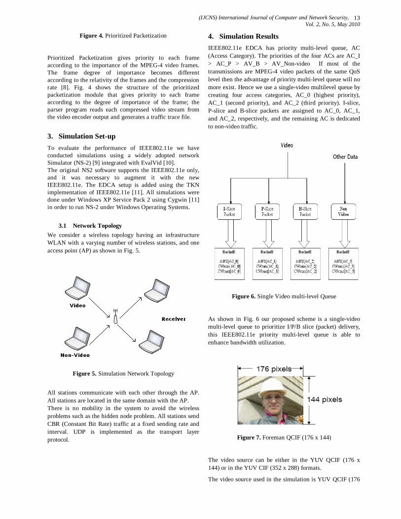
4. Simulation Results IEEE802.11e EDCA has priority multi-level queue, AC (Access Category). The priorities of the four ACs are AC_I > AC_P > AV_B > AV_Non-video If most of the transmissions are MPEG-4 video packets of the same QoS level then the advantage of priority multi-level queue will no more exist. Hence we use a single-video multilevel queue by creating four access categories, AC_0 (highest priority), AC_1 (second priority), and AC_2 (third priority). I-slice, P-slice and B-slice packets are assigned to AC_0, AC_1, and AC_2, respectively, and the remaining AC is dedicated to non-video traffic.
Figure 6. Single Video multi-level Queue
As shown in Fig. 6 our proposed scheme is a single-video multi-level queue to prioritize I/P/B slice (packet) delivery, this IEEE802.11e priority multi-level queue is able to enhance bandwidth utilization.
Figure 7. Foreman QCIF (176 x 144)
The video source can be either in the YUV QCIF (176 x 144) or in the YUV CIF (352 x 288) formats.
The video source used in the simulation is YUV QCIF (176
(IJCNS) International Journal of Computer and Network Security, Vol. 2, No. 5, May 2010
14
x 144), Foreman. Each video frame was fragmented into packets before transmission, and the maximum transmission packet size over the simulated network is 1000 bytes, Fig. 7 shows the video used in our simulations.
The video sequence has temporal resolution 30 frames per second, and GoP (Group of Pictures) pattern IBBPBBPBBPBBI. In Table 1 & Table 2 shows the Total amount of each frame/packet in the video sequence respectively.
Table 1: Amount of video frames in the video source
Table 2: Amount of video packets in the video source
In table 3 shows the simulation parameters of the simulation; we simulated two different traffics which is Video & Voice.
Table 3: Simulation parameters
Simulation Parameter
Video
Voice
I -frame P-frame B- frame
Transport Protocol
UDP
UDP
UDP
UDP
CWmin 3 7 15 7 CWmax 7 15 1023 15 AIFSN 2 3 3 4
Packet Size (bytes)
1028
1028
1028
160
Packet Interval 10 ms
10 ms
10 ms
20 ms
Data rate (kbps)
1024
1024
1024
64
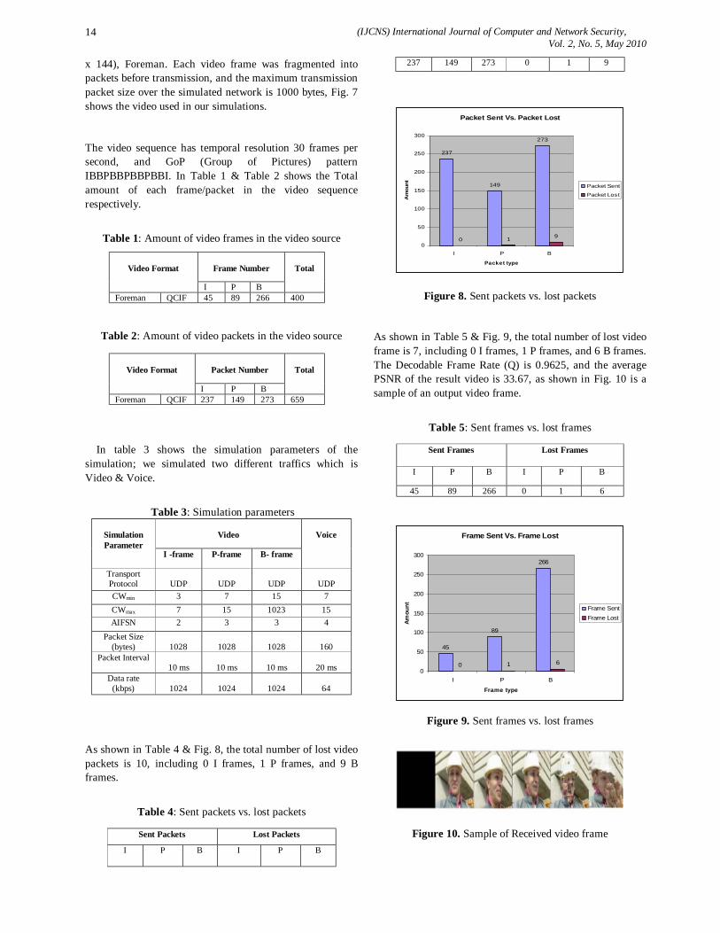
As shown in Table 4 & Fig. 8, the total number of lost video packets is 10, including 0 I frames, 1 P frames, and 9 B frames.
Table 4: Sent packets vs. lost packets
Sent Packets Lost Packets
I P B I P B
237 149 273 0 1 9
Packet Sent Vs. Packet Lost
237
149
273
0 1 9
0
50
100
150
200
250
300
I P B
Packet type
Am
ount Packet Sent
Packet Lost
Figure 8. Sent packets vs. lost packets
As shown in Table 5 & Fig. 9, the total number of lost video frame is 7, including 0 I frames, 1 P frames, and 6 B frames. The Decodable Frame Rate (Q) is 0.9625, and the average PSNR of the result video is 33.67, as shown in Fig. 10 is a sample of an output video frame.
Table 5: Sent frames vs. lost frames
Sent Frames Lost Frames
I P B I P B
45 89 266 0 1 6
Frame Sent Vs. Frame Lost
45
89
266
0 1 60
50
100
150
200
250
300
I P B
Frame type
Amou
nt Frame SentFrame Lost
Figure 9. Sent frames vs. lost frames
Figure 10. Sample of Received video frame
Video Format
Frame Number
Total
I P B Foreman QCIF 45 89 266 400
Video Format
Packet Number
Total
I P B Foreman QCIF 237 149 273 659
(IJCNS) International Journal of Computer and Network Security, Vol. 2, No. 5, May 2010
15
5. Conclusions In this paper, we evaluated a framework to improve the quality of video streaming. This framework consists of MAC-centric cross-layer architecture to allow MAC-layer to retrieve video streaming packet information (slice type), to save unnecessary packet waiting time, and a single-video multi-level queue to prioritize I/P/B slice (packet) delivery. We evaluated our simulations based on the decodable frame rate (Q) and PSNR. Through simulations, we also revealed that PSNR & decodable frame rate can evaluate the perceived quality well by an end user. Therefore, we found that the larger the Q & PSNR value, the better the video quality perceived by the end user. Simulations show that the evaluated methodology outperforms IEEE802.11e in packet loss rate, and PSNR.
References [1] IEEE 802.11e, “Wireless LAN Medium Access Control
(MAC) Enhancements for Quality of Service (QoS),” 802.11e Draft 8.0, 2004.
[2] S. Choi, “Overview of Emerging IEEE 802.11 Protocols for MAC and Above,” Telecommunications Review, Special Edition, November 2003.
[3] D. Gu, and J. Zhang, “QoS Enhancement in IEEE 802.11 Wireless Local Area Networks,” IEEE Communications Magazine, June 2003.
[4] D. Chen, D. Gu, J. Zhang, “Supporting Real-Time Traffic with QoS in IEEE802.11e Based Home Networks,” IEEE Consumer Communications and Networking Conference, January 2004.
[5] D. Gao, J. Cai, P. Bao, Z. He, “MPEG-4 Video Streaming Quality Evaluation in IEEE802.11e WLANs,” IEEE International Conference on Image Processing, September 2005.
[6] A. Ksentini, A. Gueroui, M. Naimi, “Toward an improvement of H.264 Video Transmission over IEEE802.11e through a Cross Layer Architecture,” IEEE Communications Magazine, Special Issue on Cross-Layer Protocol Engineering, January 2006.
[7] Sai Shankar N, Mihaela van der Schaar, “Performance Analysis of Video Transmission over IEEE 802.11a/e WLANs,” IEEE Transactions on Vehicular, VOL. 56, Issue 4, 2007.
[8] Pilgyu Shin, Kwangsue Chung, “A Cross-Layer Based Rate Control Scheme for MPEG-4 Video Transmission by Using Efficient Bandwidth Estimation in IEEE 802.11e,” School of Electronics Engineering, Kwangwoon University, Seoul, Korea, 2007.
[9] NS-2, http://www.isi.edu/nsnam/ns. [10] Chih-Heng, Ke, “How to evaluate MPEG video
transmission using the NS2 simulator,” EE Department, NCKU, Taiwan, 2007.
[11] S. Wiethölter and C. Hoene, “Design and Verification of An IEEE802.11e EDCF Simulation Model in ns-2.26,” Tech. Rep. TKN-03-019, Technische Universität Berlin, 2003.
[12] Cygwin, http://www.cygwin.com [13] IEEE Std 802.11e-2005, “Wireless LAN Medium
Access Control (MAC) and Physical Layer (PHY) specifications Amendment 8: Medium Access Control (MAC) Quality of Service Enhancements,” November 2005.
[14] Zhen-ning Kong, Danny H. K. Tsang, Brahim Bensaou, Deyun Gao, “Performance Analysis of IEEE802.11e
Contention-Based Channel Access,” IEEE JOURNAL ON SELECTED AREAS IN COMMUNICATIONS, VOL. 22, No. 10, December 2004.

(IJCNS) International Journal of Computer and Network Security, Vol. 2, No. 5, May 2010
16
Face Recognition Using Subspace LDA
Sheifali Gupta 1, O.P.Sahoo 2, Ajay Goel3 and Rupesh Gupta4
1 Department of Electronics & Communication Engineering, Singhania University, Rajasthan,India
2Department of Electronics & Communication Engineering, N.I.T. Kurukshetra, India,
3Department of Computer Science & Engineering Singhania University, Rajasthan, India
4Department of of Mechanical Engineering Singhania University, Rajasthan, India
Abstract: In this paper we have developed subspace LDA approach for face recognition. This approach consists of two steps; the face image is projected into the eigenface space which is constructed by PCA, and then the eigenface space projected vectors are projected into the LDA classification space to construct a linear classifier. We have focused on the effects of taking the number of significant eigen vectors in LDA approach. Experimental results using MATLAB are presented in this paper to demonstrate the viability of the proposed face recognition method. It shows that a high recognition rate is observed when the eigenface space’s dimension is small (40-60) and it is less when eigenface space’s dimension is large (175-200). It also shows that if the minimum Euclidian distance of the test image from other images is zero, then the test image completely matches the existing image in the database. If minimum Euclidian distance is non-zero but less than threshold value, then it is a known face but having different face expression else it is an unknown face.
Keywords: Face Recognition, Eigenvalues, Principle component analysis (PCA), LDA (Linear Discriminant Analysis)
1. Introduction In recent years considerable progress has been made on
the problem of face detection and recognition. The best results have been attained with frontal facial images. The problem of recognizing a human face from a general view remains largely unsolved. Biological changes such as aging cause similar problems.
An information theory approach to face recognition decomposes face images into a small set of characteristic feature images called ‘eigenfaces’, which are actually the principal components of the initial training set of face images. Then recognition is performed by projecting a new image into the subspace spanned by the eigenfaces (‘face space’) and then classifying the face by comparing its position in the face space with the positions of the known individuals [1].
2. Background and Related Work Much of the work in computer recognition of faces has
focused on detecting individual features such as eyes, nose, mouth and head outline and defining a face model by position, size and relationships among features. Eigenfaces and Fisherfaces are reference face recognition methods which build reduced subspaces in order to generate optimal features of facial images.
2.1 Principal Component Analysis PCA is a general method used for the identification of linear directions in which a set of vectors is best represented. It is commonly used as a pre-processing technique for dimensional reduction. Kirby and Sirovich used PCA in 1987 in order to obtain a reduced image space [2]. After that in 1991 Turk, Pentland, Moghaddam and Starner extended the idea to eigenspace projections in the solution of face recognition [3]. 2.2 Fisher Discriminant Analysis R. A. Fisher developed Linear/Fisher Discriminant Analysis (LDA) in 1936 [4]. Fisher Discriminant Analysis (FDA) is a powerful method for face recognition yielding an effective representation that linearly transforms the original data space into a low-dimensional feature space where the data is as well separated as possible under the assumption that the data classes are Gaussian with equal covariance structure. While PCA tries to generalize the input data to extract the features, LDA tries to discriminate the input data by dimension reduction. The Linear Discriminant Analysis searches for the best projection to project the input data on a lower dimensional space, in which the patterns are discriminated as much as possible. For this purpose, LDA tries to maximize the scatter between different classes and minimize the scatter between the input data in the same class.

(IJCNS) International Journal of Computer and Network Security, Vol. 2, No. 5, May 2010
17
3. Subspace LDA Method It is an alternative method which combines PCA and
LDA [5]. This method consists of two steps; the face image is projected into the eigenface space which is constructed by PCA, and then the eigenface space projected vectors are projected into the LDA classification space to construct a linear classifier. In this method, the choice of the number of eigenfaces used for the first step is critical; the choice enables the system to generate class separable features via LDA from the eigenface space representation. Projecting the data to the eigenface space generalizes the data, whereas implementing LDA by projecting the data to the classification space discriminates the data. Thus, Subspace LDA approach seems to be a complementary approach to the Eigenface method.
4. Experimental Results To analyze the performance of human face recognition using subspace LDA, we performed experiments on ORL databases using MATLAB. There are 10 different images of 40 distinct subjects in ORL database. For some of the subjects, the images were taken at different times, varying lighting slightly, facial expressions (open/closed eyes, smiling/non-smiling) and facial details (glasses/no-glasses). All the images are taken against a dark homogeneous background and the subjects are in up-right, frontal position (with tolerance for some side movement). The files are in .TIF file format (Tagged Image File Format). The size of each image is 92 x 112 (width x height), 8-bit grey levels. In this part of the experiments, the effect of using different number of eigenvectors while projecting the images is studied. From Fig 1, it can be observed that when the eigenface space’s dimension is small (40-60), it performs better. When the eigenface space’s dimension is large (175-200) there is a decrease in recognition rate.
Figure 1. Recognition Rate Vs Number of EigenFace
Now we have taken the Euclidean distance as a metric for face recognition. The Euclidean distance of test image from
each image in the database is calculated. The test image will match the image in the database having the minimum Euclidean distance with it. In figure 2, Euclidean distance of one test image from all the 400 images is shown. The Euclidean distance is zero with the image no. 7 in the database as clear from the figure 2. As the Euclidean distance is zero, so test image completely match the image from our database as shown in figure 3.
Figure 2. Euclidean Distance of a test image from other
images in database
Figure 3.
For another test image no. 3, Euclidean distance from other images is shown in figure 4. The minimum Euclidean distance is with the Image no.5 in the database. This distance is less than threshold value; hence it is a known face.

(IJCNS) International Journal of Computer and Network Security, Vol. 2, No. 5, May 2010
18
Figure 4.
The test image matches the image in the database having different face expression as clear from the figure 5.
Figure 6.
5. Conclusions The subspaceLDA method is a combination of eigenface
method and LDA approach. Eigenface method is used for dimension reduction to decrease the processing time and LDA approach is used for classification due to its discrimination power to enhance the recognition rate. From the observations, it is clear that a high recognition rate is observed when the eigenface space’s dimension is small (40-60) and it is less when eigenface space’s dimension is large (175-200).
It is also clear that if the minimum Euclidian distance of the test image from other images is zero, then the test image completely matches the existing image in the database. If minimum Euclidian distance is non-zero but less than threshold value, then it is a known face but having different face expression else it is an unknown face.
References [1] S.A. Rizvi, P.J. Phillips, and H. Moon, “A verification
protocol and statistical performance analysis for face recognition algorithms”, pp. 833-838, IEEE Proc. Conf. Computer Vision and Pattern Recognition (CVPR), Santa Barbara, June 1998.
[2] M.Kirby and L. Sirovich “Application of the Karhunen-Loeve procedure for the characterization of human faces". IEEE Transactions on Pattern analysis and Machine Intelligence 12 (1): 103–108. doi: 10.1109 /34.41 39
[3] A.Pentland, B.Moghaddam, T.Starner, O. Oliyide, and M. Turk (1993), “View - based and modular Eigenspaces for face recognition". Technical Report 245, M.I.T Media Lab.
[4] R.A.Fisher, “The Use of Multiple Measurements in Taxonomic Problems”, Annals of Eugenics, Vol. 7, No. 2. (1936), pp. 179-188.\
[5] P. N. Belhumeur, J. P. Hespanha and D. J. Kriegman, “Eigenfaces vs. Fisherfaces: Recognition Using Class Spesific Linear Projection”, IEEE Transactions on Pattern Analysis and Machine Intelligence, Vol. 19, No. 7, July 1997.

(IJCNS) International Journal of Computer and Network Security, Vol. 2, No. 5, May 2010
19
Travelling Salesman’s Problem: A Petri net Approach
Sunita Kumawat 1 , G.N.Purohit 2 1, 2 Department of Mathematics and statistics, Centre of Mathematical Sciences (CMS),
Banasthali University,Banasthali (Rajasthan)-304022, India. email: [email protected], [email protected]
Abstract: In this paper, we consider the Travelling salesman’s problem (TSP). Where TSP is modelled as a TSP-graph, in which each edge is treated as a parallel combination of oppositely directed edges. We model TSP-graph as a Petri Net-graph, where Petri Net- graph is an underlying graph of TSP-graph. Then solve TSP by defining suitable binary operation on elements of columns in sign incidence matrix representation of Petri Net-graph. In Petri Net-graph, we find a set of places which is both Siphon and Trap with minimum sum of capacities, whose set of input transitions equals to the set of output transitions, and both of them are equal to the set of all transitions in Petri Net. Then edges in TSP-graph corresponding to these places in Petri Net-graph will form a shortest route for the salesman to return the point of origin, after traversing all the cities exactly ones. For the solution of TSP, we describe a new algorithm, based on siphon-trap and bounded-ness property of the Petri Nets. 2000 Mathematics Subject Classification: 68R10, 90C35, 94C15. Keywords: Travelling Salesman’s Problem, Weighted Directed Graph, Spanning Cycle, Petri Net, Siphon and Trap.
1. Introduction The Travelling Salesman’s Problem (TSP) is one of the most intensely studied problems in computational mathematics [5]. Mathematical problems related to the TSP were treated in the early nineteenth century by W.R Hamilton and British mathematician T. P. Kirkman. Although there are many algorithms given for the solution of TSP [6, 7, 8, 13, 14], yet no effective solution is known for the general case for the TSP. In this paper, we address the same problem with a different approach, using Petri Net model. Here we present a new algorithm to solving a TSP using the siphon-trap and bounded-ness property of the places in the One-one Petri Net model of given TSP-graph. For the TSP we find a set of places in Petri Net, which is both Siphon and Trap [1, 3], with minimum sum of capacities, having the property that set of input transitions equals to the set of output transitions, and both of them are equal to the set of all transitions given in the Net. Then edges in TSP-graph corresponding to these places form a shortest route for the salesman. In Petri Net theory, Petri Net is a formal tool which is particularly well suited for discrete event systems. Its application has emerged from the initial seminal PhD thesis of C. A. Petri, so C.A. Petri is considered as the originator of Petri Net applications [10, 11]. The computational algorithmic aspects of graph theory are emphasized in the study of the Petri Nets. The most
interesting connections between graph theory and Petri Nets have been brought out by T. Murata [9]. This paper is organized as follows: Section 2 provides the necessary preliminaries, Section 3 formulates the problem, Section 4 describes the algorithm for TSP with illustrative example and Section 5 briefly concludes this paper. 2 . An Overview Of Petri Net Approach This section of the paper provides the necessary preliminaries for the readers who are not familiar with Petri nets. As Petri Nets are also called place-transition net (PT-Net), it is a particular kind of directed graphs together with an initial state called the initial marking. In general a Petri Net is an underlying graph of any directed graph, which is in essence a directed bipartite graph with two types of nodes called places and transitions. The arcs are either from places to transitions (output of places) or from transitions to places (input of places). In the Petri Net graph a place is denoted by a circle, a transition by a box or a bar and an arc by a directed line. A Petri Net is a PT-Net with tokens assigned to its places denoted by black dots, and the token distribution over its places is done initially by a marking function denoted by M0. A token is interpreted as a command given to a condition (place) for the firing of an event (transition). An event can happen, when its all input conditions are fulfilled, See Fig.1.
Figure 1.
There are many subclasses of Petri Nets such as One-one Petri Nets, free choice Petri Nets, colored and stochastic Petri Nets etc. Here we introduce only One-one Petri Net, as it is an ordinary Petri Net such that each place P has exactly one input transition and one output transition having weight one on each edge, but we ignore these weights generally in the model representation of the Net PN. One-one Petri Net is also called as Marked Graph [4]. In our paper standard notation PN is treated as One-one Petri Net. More detailed and formal description of Petri Nets is given in [2, 9, 10,

(IJCNS) International Journal of Computer and Network Security, Vol. 2, No. 5, May 2010
20
15]. We include here some basic definitions, which are relevant to this paper. Definition 2.1: A place-transition net (PT-Net) is a quadruplet PN = ⟨P, T, F, W⟩, where P is the set of places, T is the set of transitions, such that P ∪ T≠∅ and P ∩ T=∅, F⊆ (P x T) ∪ (T x P) is the set of arcs and W: F à1, 2 ... is the weight function. PN is said to be an ordinary PT-Net if and only if W: Fà 1. A marking is a function M0: Pà 0, 1, 2 ..., which distributes the tokens to the places initially. Here M0 (p) is the number of tokens in the place p at initial marking M0, it is a non- negative integer less then or equal to the capacity of the place. Capacity of the place is defined as the capability of holding the maximum no. of tokens at any reachable marking M from M0. A marking M is said to reachable to M0 if there exist a firing sequence σ = t1, t2… tn such that M can be obtained from M0 as firing of transitions t1, t2,…, tn. A Petri Net structure PN = ⟨P, T, F, W⟩ without any specific initial marking is denoted by PN and Petri Net with the given initial marking is denoted by ⟨ PN, M0⟩. *x and x* are the set of input transitions (or places) and the set of output transitions (or places) respectively, as x∈ P (or T). Here | *x | and | x* | stands for number of the input transitions (or places) and the output transitions (or places) respectively. Thus a One-one Petri Net is an ordinary PT-Net such that ∀ p ∈ P: |*p|=|p*| =1, i.e., the number of the input transitions for p ∈ P equals to the number of the output transitions and both of them are equal to one. For a PT-Net, a path is a sequence of nodes ρ = ⟨ x1, x2… xn ⟩ where (xi, xi+1) ∈F for i = 1, 2… n-1. ρ is said to be elementary if and only if it does not contain the same node more than once and a cycle is a sequence of places ⟨ p1 , p2 , …pn ⟩ such that there exist t1, t2,…, tn ∈ T : ⟨ p1, t1, p2, t2,…., pn , tn ⟩ forms an elementary path and (tn, p1) ∈F. Definition 2.2: For a PT-Net ⟨PN, M0⟩, a place p is said to be k-bounded (or bounded by k) where k∈ R+, if and only if M0 (p) < k., denotes the capacity of the place in the Net. (PN, M0⟩ is said to be k-bounded if and only if every place is k-bounded. Definition 2.3: A non-empty subset of places S is called a Siphon if *p⊆ p* ∀ p∈S denoted also *S⊆ S*; i.e., every transition having an output place in S has an input place in S. Likewise a non-empty subset of places Q is called a Trap if p*⊆ *p ∀ p∈Q denoted also Q* ⊆ *Q; i.e., every transition having an input place in Q has an output place in Q. 3. Problem Formulation: Travelling Salesman’s Problem (TSP) For a given network of cities and the cost of travel between each pair of them, the Travelling Salesman’s Problem or TSP for short, is to find the shortest route for the salesman, visiting to all of the cities exactly ones and returning to the starting point. In the standard version of TSP, the travel costs or distances are symmetric in the sense that travelling from city X to city Y costs just as much as travelling from Y to X. Any round-trip tour that
goes through every city exactly once is a feasible tour with a given cost, if it is smaller than the other minimum cost tour. 3.1 Modelling TSP as a Graph (TSP-graph): A pair G = V, E, where V= v1,v2,v3,…,vn is the set of vertices and E = e1,e2,…,em is the set of edges such that each edge ei having some weights wi∈W, where W:Eà R+
is the weight function and wi =w(ei) is the weight associated with edge ei . Further when the edges vi vj and vj vi are considered different then G=V,E is called a weighted directed graph. In weighted directed graph, a directed cycle is a closed sequence of directed edges without repetition of vertices except terminals and it said to be Spanning if it contains all the vertices of the graph. If any edge from the sequence is deleted then cycle becomes open. Thus solving a TSP amounts to finding a minimum weight spanning cycle. As an illustration we consider a weighted graph on four vertices denoting the four cities A, B, C, D, where each city has a direct link with the other three. The numbers (weights) associated with the edges denotes the physical distance between the cities, See Fig. 2. We construct a directed weighted graph (TSP-graph) of the same graph in Fig. 3.
Distance between two cities in Fig.3 can be represented in terms of adjacency matrix as depicted below:
V1 V2 V3
V4
V1 --- 128 163 298
V2 128 --- 98 206 V3 163 98 --- 137 V4 298 206 137 ---
TSP- Graph
e1 V1
V3
V2
V4
e2 e8
e3
e7
e4
e5
e10
e9 e11
e12
e6
Figure 3.
A
D B
C Figure 2. Network of cities
128
206
163
298
137
98
(IJCNS) International Journal of Computer and Network Security, Vol. 2, No. 5, May 2010
21
3.2 Modelling TSP-graph as a Petri Net A Petri Net PN is modelled from TSP-graph given in Fig. 3 as follows: edges es are transformed into places ps and vertices vk are transformed into transitions tk so that the place ps has an input from a transition ti, and an output to a transition tj, if es is an directed edge vi vj in graph, then weights (distance between two cities) of es’s are replaced by capacities ks of corresponding places ps and number of tokens for places ps‘s is the value of sk . Fig. 4 in Appendix (1), shows the One-one Petri Net model say PN, of the TSP-graph, having the set of transitions T= t1 t2, t3, t4 and the set of places is P = p1, p2,…,p12 corresponding to the set of verticesv1,v2,v3,v4 and the set of edges e1,e2,…,e12 respectively in the given TSP-graph. For the sake of clarity, we observe that t1 is the input transitions for the places p2, p7, p10 and the output transition for the places p1, p8, and p9. Similarly p1 is the input place for the transition t1 and output place for the transition t4. Using this same procedure, we find a set of the places in Net which is both siphon and trap with minimum sum of capacities, whose set of the input transitions equals to the set of output transitions and both of them are equal to the set of all transitions in the Net PN. 4. Description of algorithm for Travelling Salesman’s Problem As in above we model the TSP-graph as a Petri Net-graph. Now here we present an algorithm for solving the Travelling Salesman’s Problem. For the description of the algorithm for TSP; we introduce some new notations as follows: In a Petri Net PN with n-transitions and m-places, the sign incidence matrix I = [aij] is the n x m matrix, whose entries are defined as, aij = + if place j is an output place of transition i. aij = - if place j is an input place of transition i. aij = ± if place j is both input and output places of transition i, (i.e., transition i and place j form a self loop)
aij = 0 otherwise.
As an illustration, the Sign incidence matrix I of PN is: p1 p2 p3 p4 p5 p6 p7 p8 p9 p10 p11 p12
t1 - + 0 0 0 0 + - - + 0 0
t2 0 0 0 0 + - - + 0 0 + - t3 0 0 + - - + 0 0 + - 0 0 t4 + - - + 0 0 0 0 0 0 - +
Hare we introduce a commutative binary operation, denoted by ⊕ on the set U= (0, +, - ,±). ⊕ defined as following: + ⊕ - = ± (i.e., ‘+’ entry is said to be neutralized by adding a ‘–‘entry to get a ‘±’ entry). a ⊕ a = a ∀ a∈U ± ⊕ a = ± ∀ a∈ 0 ⊕ a = a ∀ a∈U For the Travelling salesman’s problem, we choose a subset of k places X = p1, p2…pk in sign incidence matrix
I of PN, which is both siphon and trap and also *X= X* = T, i.e., set of the input transitions of X is equals to the set of output transitions of X, and both of them equal to the set of all transition in T. This equality holds only if the addition under the operation ⊕, of the k column vectors say C1, C2, C3,…, Ck i.e., C1 ⊕ C2⊕ C3⊕…..⊕ Ck contains only ± entries everywhere, where Cj , j = 1, 2... k, denotes the column vector corresponding to the place pj in I. Now let C1 ⊕ C2⊕ C3⊕…..⊕ Ck will be a column vector denoted by γ = [γi] where γi denotes the i th element of the column vector γ, have as elements from set U. Then from the definition of I under the operation⊕, we interprets about γi as. γi = 0 means no place in X is an input or output place of transition i. γi = - means some place in X is an input place of transition i.γi = + means some place in X is an output place of transition i. γi = ± means some place in X is an input place as well as output place for transition i. From the above it can be seen that every transition having an output place in X has an input place in X only if γi ≠ +, and likewise every transition having an input place in X has an output place in X only if γi ≠-. So X is both siphon and trap if and only if γ has either 0 or ± entries. And if γ has only ± entries everywhere, then the places corresponding to columns C1, C2, C3,…, Ck in C1 ⊕ C2⊕ C3⊕…..⊕ Ck forms a set of places, which is both siphon and trap, whose input transitions equals to the output transitions and both of them are equal to the set of all transitions T, with having some capacities. We select only those set of places X such that *X = X* = T, having minimum sum of capacities among all. Algorithm discussed below, gives us a siphon–trap set of places X with minimum sum of capacities, having the property *X = X* = T, whose corresponding edges in TSP-graph will form a shortest route for the salesman. ALGORITHM: Input Sign incidence matrix I of order n x m.
Step 1 Select Cj, the first column in the sign incidence matrix I having ‘+’ entry whose corresponding place and capacity is denoted as PLACEj and CAPACITYj Set recursion level r to 1 Set Vjr = Cj Set PLACEjr = PLACEj; Set CAPACITYjr =CAPACITYj; Set X =∅, W=∅, Sum =0 and K =∅.
Step 2 If Vjr has a ‘±’ entry at the ith row then PLACEjr is a self loop with transition i, Go to Step 5.
Step 3 If Vjr has a ‘+’ entry in the kth row find a column Cs which contains a ‘–‘entry at kth row.
(i) If no such column Cs exists then go to Step 5. (ii) If such Cs exists, add it to Vjr to obtain Vj(r+1) = Vjr ⊕
Cs, containing a ‘±’ entry at kth row. Then PLACEj(r+1) = PLACEjr ∪ PLACEs

(IJCNS) International Journal of Computer and Network Security, Vol. 2, No. 5, May 2010
22
CAPACITYj(r+1) = CAPACITYjr ∪ CAPACITYs (iii) Repeat this step for all neutralizing columns Cs. This
gives a new set of Vj(r+1)’s, PLACEj(r+1)‘s and CAPACITYj(r+1)
Step 4 Increase r by 1, Repeat Step 3 until there are no ‘+’entries in each Vjr = C1 ⊕ C2⊕ C3⊕…..⊕ Cjr.
Step 5 Any Vjr with all entries as ‘±’ represents both siphon and trap such that their input transitions equal to the output transitions and both of them equal to the set of all transitions T. X = X ∪ PLACEjr
K= K ∪ CAPACITYjr W=Sum + Sumw K, where Sumw K is the sum of the capacities in the set K, Store it any other set and compare it to minimum weight set at each iteration. Step 6 Delete Cj
j = j + 1 Go to Step 1. Output: Set X has places both siphon and trap such that their input transitions equal to the output transitions and both of them equal to the set of all transitions T with minimum sum of capacities. Whose corresponding edges set in TSP-graph, forms a shortest route for the salesman. As an illustration consider the graph in Fig 2. Step 1 Select first column having ‘+’ entry. Here is C1, then
11V =
+
−
00 ; PLACE11 = pl;
CAPACITY11 = 137 Steps 2, 3 and 4, V11 has a ‘+’ entry at 4th row. The neutralizing columns are C2, C3 and C11.
)1(12V = 11V ⊕ C2 =
+
−
00 ⊕
−
+
00 =
±
±
00 ;
PLACE )1(12 = pl , p2; CAPACITY )1(
12 =137,137
)2(12V = 11V ⊕ C3 =
+
−
00 ⊕
−+00
=
±+
−0 ;
PLACE )2(12 = pl, p3; CAPACITY )2(
12 = 137,206
)3(12V = 11V ⊕ C11 =
+
−
00 ⊕
−
+0
0
=
±
+−
0;
PLACE )3(12 = pl, p11; CAPACITY )3(
12 = 137,298
)2(12V has ‘+’ entry at 3rd row. The neutralizing columns
are C4, C5 and C10.
)1(13V = )2(
12V ⊕ C4 =
±+
−0 ⊕
+−00
=
±±
−0 ;
PLACE )1(13 = pl,p3, p4; CAPACITY )1(
13 = 137,206,206
)2(13V = )2(
12V ⊕ C5 =
±+
−0 ⊕
−+
0
0
=
±±+−
;
PLACE )2(13 =pl, p3, p5; CAPACITY )2(
13 = 137, 206,128
)3(13V = )2(
12V ⊕ C10 =
±+
−0 ⊕
−
+
0
0 =
±±
±0 ;
PLACE )3(13 = pl, p3, p10; CAPACITY )3(
13 = 137, 206, 98
)3(12V has ‘+’ entry at 2nd row. The neutralizing column is
C6, C7 and C12.
)4(13V = )3(
12V ⊕ C6 =
±
+−
0 ⊕
+−
0
0
=
±+±−
;
PLACE )4(13 = pl, p11, p6; CAPACITY )4(
13 = 137,298,128
)5(13V = )3(
12V ⊕ C7 =
±
+−
0 ⊕
−+
00
=
±
±±
0;
PLACE )5(13 = pl , p11, p7; CAPACITY )5(
13 = 137,298,163
)6(13V = )3(
12V ⊕ C12 =
±
+−
0 ⊕
+
−0
0
=
±
±−
0;
PLACE )6(13 = pl, p11, p12; CAPACITY )6(
13 = 137,298,298
)1(13V and )6(
13V has no ‘+’ entry , also all the entries are not ‘±’ only, but those sets which have all entries ‘±’ or ‘0’ are both siphon and trap ( as )1(
12V , )3(13V and )5(
13V )
)2(13V has ‘+’ entry at 2rd row. The neutralizing columns are
C6, C7, and C12.
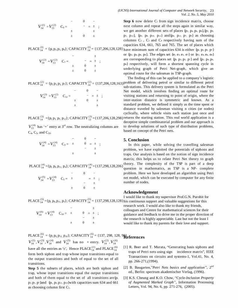
(IJCNS) International Journal of Computer and Network Security, Vol. 2, No. 5, May 2010
23
)1(14V = )2(
13V ⊕ C6 =
±±+−
⊕
+−
0
0
=
±±±−
;
PLACE )1(14 = pl, p3, p5, p6; CAPACITY )1(
14 = 137,206,128,128
)2(14V = )2(
13V ⊕ C7 =
±±+−
⊕
−+
00
=
±±±±
;
PLACE )2(14 = pl, p3, p5, p7; CAPACITY )2(
14 = 137,206,128,163
)3(14V = )2(
13V ⊕ C12 =
±±+−
⊕
+
−0
0
=
±±±−
;
PLACE )3(14 =pl, p3, p5, p12; CAPACITY )3(
13 =137,206,128,298
)4(13V has ‘+’ entry at 3rd row. The neutralizing columns are
C4, C5, and C10.
)4(14V = )4(
13V ⊕ C4 =
±+±−
⊕
+−00
=
±±±−
;
PLACE )4(14 =pl, p6, p11, p4; CAPACITY )4(
14 =137,298,128,206
)5(14V = )4(
13V ⊕ C5 =
±+±−
⊕
−+
0
0
=
±±±−
;
PLACE )5(14 =pl, p6, p11, p5; CAPACITY )5(
14 = 137,298,128,128
)6(14V = )4(
13V ⊕ C10 =
±+±−
⊕
−
+
0
0 =
±±±±
;
PLACE )6(14 = pl, p6, p11, p10; CAPACITY )6(
14 = 137, 298, 128, 98 )1(
14V , )3(14V , )4(
14V and )5(14V has no + entry. )2(
14V , )6(14V
have all the entries as ‘±’, Hence PLACE )2(14 and PLACE )6(
14 form both siphon and trap whose input transitions equal to the output transitions and both of equal to the set of all transitions. Step 5 the subsets of places, which are both siphon and trap, whose input transitions equal the output transitions and both of them equal to the set of all transitions arepl, p3, p5, p7and pl,, p6, p11, p10with capacities sum 634 and 661 as choosing column first C1.
Step 6 now delete C1 from sign incidence matrix, choose next column and repeat all the steps again in similar way, we get another different sets of places p2, p4, p6, p8,p2, p9,
p5, p12, p3, p8, p10, p12 andp4, p11, p7, p9 as choosing columns C2 , C3 and C4 respectively having sum of the capacities 634, 661, 765 and 765. The set of places which have minimum sum of capacities 634 is either pl, p3, p5, p7 or p2, p4, p6, p8. The edges set el, e3, e5, e7 or e2, e4, e6, e8 are corresponding to places set pl, p3, p5, p7 and p2, p4, p6, p8 respectively, will form a shortest spanning cycle in underlying graph of Petri Net-graph, which give an optimal route for the salesman in TSP-graph. The finding of this can be applied to a company’s logistic problem of delivering petrol or similar to different petrol sub-stations. This delivery system is formulated as the Petri Net model, which involves finding an optimal route for visiting stations and returning to point of origin, where the inter-station distance is symmetric and known. As a standard problem, we defined it simply as the time spent or distance traveled by salesman visiting n cities (or nodes) cyclically, where vehicle visits each station just once and returns the starting station. This real world application is a deceptive simple combinatorial problem and our approach is to develop solutions of such type of distribution problems, based on concept of the Petri nets. 5. Conclusion In this paper, while solving the travelling salesman problem, we have exploited the potentials of siphons and traps. Our analysis is based on the notion of sign incidence matrix; this helps us to relate Petri Net theory to graph theory. The complexity of the TSP is part of a deep question in mathematics, as TSP is a NP- complete problem. Here we have developed an algorithm using Petri net model, which can be executed by computer for any finite number of nodes. Acknowledgement I would like to thank my supervisor Prof.G.N. Purohit for his continuous support and valuable suggestions for this research work. I would also like to thank my friends, colleagues and Centre for mathematical sciences for their guidance and feedback to drive me in the proper direction of the research is highly appreciable. Last but not the least I would like to thank my parents for their love and support. References [1] R. Boer and T. Murata, “Generating basis siphons and
traps of Petri nets using sign incidence matrix”, IEEE Transactions on circuits and systems-1, Vol.41, No. 4, pp. 266-271,(1994).
[2] B. Baugarten,”Petri Nets basics and application” , 2nd ed., Berlin: spectrum akademischer Verlag, (1996).
[3] K.S. Cheung and K.O. Chow, “Cycle-Inclusion Property of Augmented Marked Graph” , Information Processing Letters, Vol. 94, No. 6, pp. 271-276, (2005).
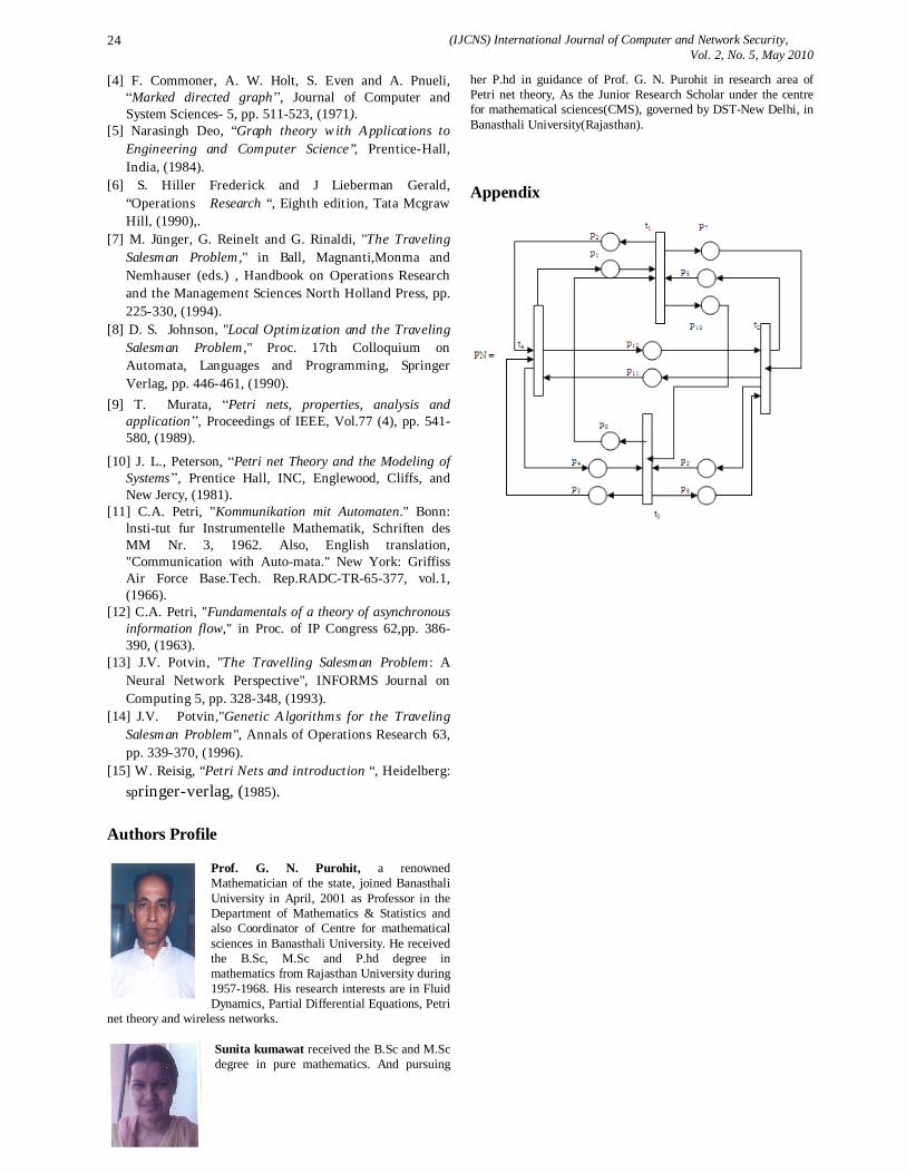
(IJCNS) International Journal of Computer and Network Security, Vol. 2, No. 5, May 2010
24
[4] F. Commoner, A. W. Holt, S. Even and A. Pnueli, “Marked directed graph” , Journal of Computer and System Sciences- 5, pp. 511-523, (1971).
[5] Narasingh Deo, “Graph theory with Applications to Engineering and Computer Science”, Prentice-Hall, India, (1984).
[6] S. Hiller Frederick and J Lieberman Gerald, “Operations Research “, Eighth edition, Tata Mcgraw Hill, (1990),.
[7] M. Jünger, G. Reinelt and G. Rinaldi, "The Traveling Salesman Problem," in Ball, Magnanti,Monma and Nemhauser (eds.) , Handbook on Operations Research and the Management Sciences North Holland Press, pp. 225-330, (1994).
[8] D. S. Johnson, "Local Optimization and the Traveling Salesman Problem," Proc. 17th Colloquium on Automata, Languages and Programming, Springer Verlag, pp. 446-461, (1990).
[9] T. Murata, “Petri nets, properties, analysis and application” , Proceedings of IEEE, Vol.77 (4), pp. 541-580, (1989).
[10] J. L., Peterson, “Petri net Theory and the Modeling of Systems” , Prentice Hall, INC, Englewood, Cliffs, and New Jercy, (1981).
[11] C.A. Petri, "Kommunikation mit Automaten." Bonn: lnsti-tut fur Instrumentelle Mathematik, Schriften des MM Nr. 3, 1962. Also, English translation, "Communication with Auto-mata." New York: Griffiss Air Force Base.Tech. Rep.RADC-TR-65-377, vol.1, (1966).
[12] C.A. Petri, "Fundamentals of a theory of asynchronous information flow," in Proc. of IP Congress 62,pp. 386-390, (1963).
[13] J.V. Potvin, "The Travelling Salesman Problem: A Neural Network Perspective", INFORMS Journal on Computing 5, pp. 328-348, (1993).
[14] J.V. Potvin,"Genetic Algorithms for the Traveling Salesman Problem", Annals of Operations Research 63, pp. 339-370, (1996).
[15] W. Reisig, “Petri Nets and introduction “, Heidelberg: springer-verlag, (1985).
Authors Profile
Prof. G. N. Purohit, a renowned Mathematician of the state, joined Banasthali University in April, 2001 as Professor in the Department of Mathematics & Statistics and also Coordinator of Centre for mathematical sciences in Banasthali University. He received the B.Sc, M.Sc and P.hd degree in mathematics from Rajasthan University during 1957-1968. His research interests are in Fluid Dynamics, Partial Differential Equations, Petri
net theory and wireless networks.
Sunita kumawat received the B.Sc and M.Sc degree in pure mathematics. And pursuing
her P.hd in guidance of Prof. G. N. Purohit in research area of Petri net theory, As the Junior Research Scholar under the centre for mathematical sciences(CMS), governed by DST-New Delhi, in Banasthali University(Rajasthan). Appendix

(IJCNS) International Journal of Computer and Network Security, Vol. 2, No. 5, May 2010
25
PET/CT and MR Image Registration using Normalized Cross Correlation Algorithm and
Spatial Transformation Techniques
1 B.Balasubramanian 2 Dr. K. Porkumaran
1Associate Professor, Sri Ramakrishna Engg. College, Affiliated to Anna University Coimbatore, India 2Vice Principal, Dr.NGP Institute of Technology, Affiliated to Anna University Coimbatore, India
[email protected], [email protected]
Abstract: This paper presents the current status of PET/CT brain image registration. Registration of brain images is a more complex problem, Automatic registration, based on computer programs, might, however, offer better accuracy and repeatability and save time. Computed Tomography (CT) is used for the attenuation correction of Positron Emission Tomography (PET) to enhance the efficiency of data acquisition process and to improve the quality of the reconstructed PET data in the brain. Due to the use of two different modalities, chances of misalignment between PET and CT images are quite significant. Template matching is used for applications in image processing. Cross Correlation is the basic statistical approach to image registration. It is used for template matching or pattern recognition. Template can be considered a sub-image from the reference image, and the image can be considered as a sensed image. The objective is to establish the correspondence between the reference image and sensed image. It gives the measure of the degree of similarity between an image and template. This paper describes medical image registration by template matching based on Normalized Cross-Correlation (NCC) using Cauchy-Schwartz inequality.
Keywords: Positron Emission Tomography (PET), Computed Tomography (CT), Magnetic Resonance (MR), Normalized Cross-Correlation (NCC) 1. Introduction
Image registration is the process of overlaying two or more images of the same scene taken at different times, from different viewpoints, and/or by different sensors. It geometrically aligns two images—the reference and sensed images. The present differences between images are introduced due to different imaging conditions. Image registration is a crucial step in all image analysis tasks in which the final information is gained from the combination of various data sources like in image fusion, change detection, and multichannel image restoration. Typically, registration is required in remote sensing (multispectral classification, environmental monitoring, change detection, weather forecasting, creating super-resolution images, integrating information into geographic information systems, in medicine (combining computer tomography (CT) and NMR data to obtain more complete information about the patient, monitoring tumor growth, treatment verification, comparison of the patient’s data with anatomical atlases), in cartography (map updating), and in
computer vision (target localization, automatic quality control), to name a few. During the last decades, image acquisition devices have undergone rapid development and growing amount and diversity of obtained images invoked the research on automatic image registration. A comprehensive survey of image registration methods was published in 1992 by Brown . According to the database of the Institute of Scientific Information, in the last 10 years more than 1000 papers were published on the topic of image registration. Methods published before 1992 that became classic or introduced key ideas, which are still in use, are included as well to retain the continuity and to give complete view of image registration research.
Biomedical imaging based on different physical principles has played a more and more important role in medical diagnosis. Multiform methods of image diagnosis provide doctors and clinicians with various anatomical and functional information to carry out exact diagnosis and effective treatment. Image registration is the process of combination the different sets of data of the same object, which come from different modalities (CT, MRI, SPECT, PET etc.). Pre-processing algorithms improve image quality and image registration algorithms transform the object of images into one coordinate system.
Nowadays, medical image diagnosis is considered as one of the fields taking advantage of high-technology and modern instrumentation. DSA, Ultrasound, CT, MRI, SPECT, PET etc. have played an important role in diagnosis, research, and treatment. In general, there are two basic types of medical images [1]: functional images (such as SPECT or PET scans), which provide physiological information, and anatomical images (such as X-ray, Ultrasound, CT or MRI), which provide anatomic structure of the body.The combination process consists of alignment (registration) and data fusion steps. After the combination process, the physician could use his knowledge to determine which anatomical areas are normal or abnormal in their functional characteristics.
2. Image Registration Methodology
(IJCNS) International Journal of Computer and Network Security, Vol. 2, No. 5, May 2010
26
Figure 1. Concept of Image registration Image registration, as it was mentioned above, is
widely used in remote sensing, medical imaging, computer vision etc. In general, its applications can be divided into four main groups according to the manner of the image acquisition: Different viewpoints (multiview analysis). Images of the same scene are acquired from different viewpoints. The aim is to gain larger a 2D view or a 3D representation of the scanned scene. Examples of applications: Remote sensing—mosaicing of images of the surveyed area. Computer vision—shape recovery (shape from stereo). Different times (multitemporal analysis). Images of the same scene are acquired at different times, often on regular abasis, and possibly under different conditions. The aim is to find and evaluate changes in the scene which appeared between the consecutive image acquisitions. Examples of applications: Remote sensing—monitoring of global land usage, landscape planning. Computer vision—automatic change detection for security monitoring, motion tracking. Medical imaging - monitoring of the healing therapy, monitoring of the tumor evolution. Different sensors (multimodal analysis) - Images of the same scene are acquired by different sensors. The aim is to integrate the information obtained from different source streams to gain more complex and detailed scene representation.
Examples of applications: Remote sensing—fusion of information from sensors with different characteristics like panchromatic images, offering better spatial resolution, color/multispectral images with better spectral resolution, or radar images independent of cloud cover and solar illumination. Medical imaging—combination of sensors recording the anatomical body structure like magnetic resonance image (MRI), ultrasound or CT with sensors monitoring functional and metabolic body activities like positron emission tomography (PET), single photon emission computed tomography (SPECT) or magnetic resonance spectroscopy (MRS). Results can be applied, for instance, in radiotherapy and nuclear medicine. Scene to model registration. Images of a scene and a model of the scene are registered. The model can be a computer representation of the scene, for instance maps or digital elevation models (DEM) in GIS, another scene with similar content (another patient), ‘average’ specimen, etc. The aim is to localize the acquired image in the scene/model and/or to compare them. Examples of applications: Remote sensing—registration of aerial or satellite data into maps or other GIS layers. Computer vision—target template matching with real-time images, automatic quality
inspection. Medical imaging— comparison of the patient’s image with digital anatomical atlases, specimen classification. Due to the diversity of images to be registered and due to various types of degradations it is impossible to design a universal method applicable to all registration tasks. Every method should take into account not only the assumed type of geometric deformation between the images but also radiometric deformations and noise corruption, required registration accuracy and application-dependent data characteristics.
The detection methods should have good
localization accuracy and should not be sensitive to the assumed image degradation. In an ideal case, the algorithm should be able to detect the same features in all projections of the scene regardless of the particular image deformation. Physically corresponding features can be dissimilar due to the different imaging conditions and/or due to the different spectral sensitivity of the sensors. The choice of the feature description and similarity measure has to consider these factors. The feature descriptors should be invariant to the assumed degradations. Simultaneously, they have to be discriminable enough to be able to distinguish among different features as well as sufficiently stable so as not to be influenced by slight unexpected feature variations and noise. The matching algorithm in the space of invariants should be robust and efficient. Single features without corresponding counterparts in the other image should not affect its performance. The type of the mapping functions should be chosen according to the a priori known information about the acquisition process and expected image degradations. If no a priori information is available, the model should be flexible and general enough to handle all possible degradations which might appear. The accuracy of the feature detection method, the reliability of feature correspondence estimation, and the acceptable approximation error need to be considered too. Moreover, the decision about which differences between images have to be removed by registration has to be done. It is desirable not to remove the differences we are searching for if the aim is a change detection. This issue is very important and extremely difficult. Finally, the choice of the appropriate type of resampling technique depends on the trade-off between the demanded accuracy of the interpolation and the computational complexity.
3. PET/CT Image Processing Steps The PET and CT data are acquired using a GE
discovery STE scanner and exported as DICOM images for the post processing. The specifications and the parameters of the acquisition device and the PET and CT data are provided in [5]. The PET and CT images are aligned as described below. 3.1 Image Segmentation
In the first step of the segmentation process, the image data is low pass filtered to smooth out the boundary of the brain in the PET as well as the CT images. To segment the brain in the PET images, adaptive thresholding
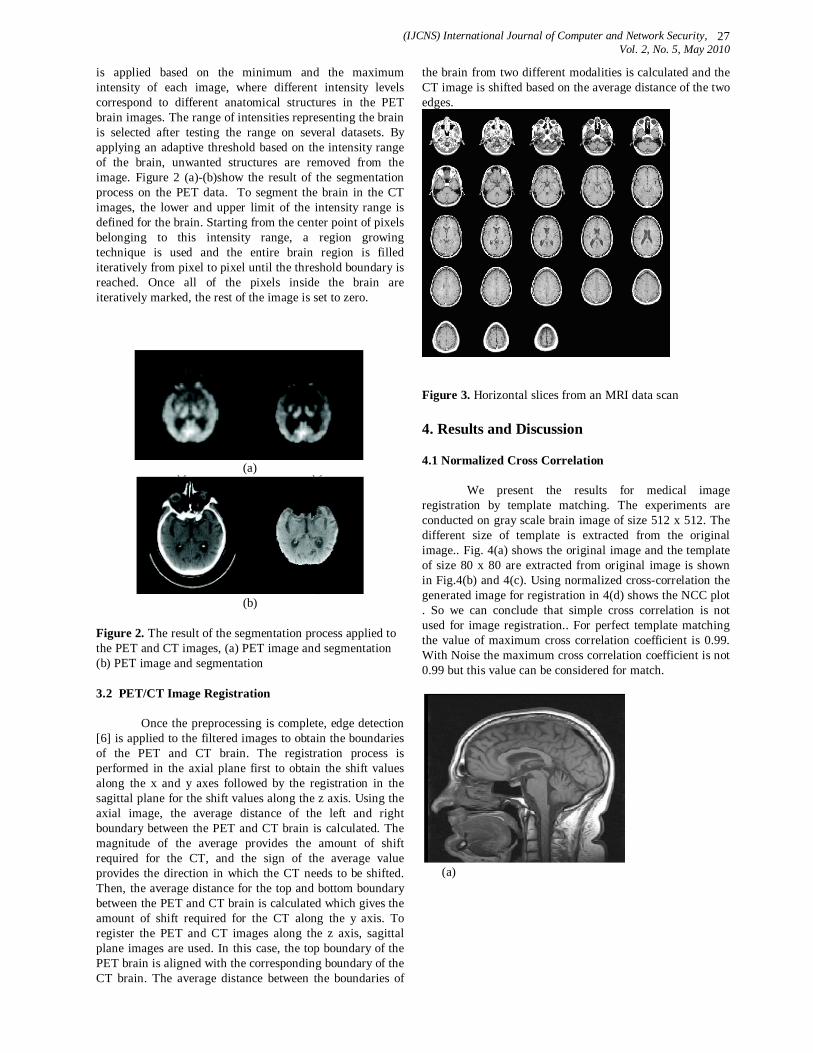
(IJCNS) International Journal of Computer and Network Security, Vol. 2, No. 5, May 2010
27
is applied based on the minimum and the maximum intensity of each image, where different intensity levels correspond to different anatomical structures in the PET brain images. The range of intensities representing the brain is selected after testing the range on several datasets. By applying an adaptive threshold based on the intensity range of the brain, unwanted structures are removed from the image. Figure 2 (a)-(b)show the result of the segmentation process on the PET data. To segment the brain in the CT images, the lower and upper limit of the intensity range is defined for the brain. Starting from the center point of pixels belonging to this intensity range, a region growing technique is used and the entire brain region is filled iteratively from pixel to pixel until the threshold boundary is reached. Once all of the pixels inside the brain are iteratively marked, the rest of the image is set to zero.
(a)
(b)
Figure 2. The result of the segmentation process applied to the PET and CT images, (a) PET image and segmentation (b) PET image and segmentation 3.2 PET/CT Image Registration
Once the preprocessing is complete, edge detection [6] is applied to the filtered images to obtain the boundaries of the PET and CT brain. The registration process is performed in the axial plane first to obtain the shift values along the x and y axes followed by the registration in the sagittal plane for the shift values along the z axis. Using the axial image, the average distance of the left and right boundary between the PET and CT brain is calculated. The magnitude of the average provides the amount of shift required for the CT, and the sign of the average value provides the direction in which the CT needs to be shifted. Then, the average distance for the top and bottom boundary between the PET and CT brain is calculated which gives the amount of shift required for the CT along the y axis. To register the PET and CT images along the z axis, sagittal plane images are used. In this case, the top boundary of the PET brain is aligned with the corresponding boundary of the CT brain. The average distance between the boundaries of
the brain from two different modalities is calculated and the CT image is shifted based on the average distance of the two edges.
Figure 3. Horizontal slices from an MRI data scan 4. Results and Discussion 4.1 Normalized Cross Correlation
We present the results for medical image registration by template matching. The experiments are conducted on gray scale brain image of size 512 x 512. The different size of template is extracted from the original image.. Fig. 4(a) shows the original image and the template of size 80 x 80 are extracted from original image is shown in Fig.4(b) and 4(c). Using normalized cross-correlation the generated image for registration in 4(d) shows the NCC plot . So we can conclude that simple cross correlation is not used for image registration.. For perfect template matching the value of maximum cross correlation coefficient is 0.99. With Noise the maximum cross correlation coefficient is not 0.99 but this value can be considered for match.
(a)

(IJCNS) International Journal of Computer and Network Security, Vol. 2, No. 5, May 2010
28
(b) (c)
050
100150
200250
0
100
200
300-0.4
-0.2
0
0.2
0.4
0.6
(d) Figure 4. (a) Original image (b), (c)Templates (d) NCC Plot
The misregistration between PET and CT is the major drawback for the CT based attenuation correction of the PET. In PET/CT studies of the human brain, the misregistration occurs mainly due to the physical motion of the patient, as most patients are unable to keep their heads still during the entire exam. The misregistration between the PET and CT brain geometries results in erroneous attenuation correction parameters for the PET reconstruction. The reconstructed PET images obtained using the misaligned CT attenuation map show areas of abnormal metabolic activity in the brain, where the PET brain is projected outside the CT brain. One approach to address the PET/CT misalignment problem is to repeat the CT scan of the brain in case of a misalignment between the PET and the original CT. In this approach, the PET and CT is downloaded to the processing unit and overlaid. If the brains geometries of the PET are CT align properly, then this CT is used for the reconstruction of the PET. However, if the PET and CT have a significant misregistration, then the patient has to go through another CT scan of the brain. In this case, the patient is exposed to an unnecessary radiation dose that can be avoided if software-aligned PET and CT is used. Also, this process can be very time-consuming and inefficient in terms of clinical resources. In contrast, software based PET/CT brain registration has the advantage of being fast with no need for operator intervention, which increases the potential for routine clinical application. Only one CT scan is needed in this case, which is aligned with the PET and then used as the attenuation correction map. This approach also reduces the radiation dose.
The original PET image and its transformed versions are shown in Figure 5. The original image is shown in Fig,5(a). Fig. 5(b) shows the affine transformed image.
The image in Fig.5(c) is obtained by applying projective transformation to the original image
(a) (b)
(c) Figure 5. a) original image b) affine transform c) projective transform The MR image in various views using rigid registration is shown in Figure 6. Fig. 6(a) shows the coronal view. Fig.6(b) and (c) shows the sagittal and axial views of an MR image
(a) (b)
(c) Figure 6. a) coronal view b) sagittal view c) axial view 5. Conclusion
Image registration is an important task that enables comparative analysis of images acquired at different occasions. We presented a simple and fast registration method that can be applied to 3DMR images of the brain. It is based on the normalized cross correlation and spatial transformation techniques. We have described a algorithm based on Normalized Cross-Correlation (NCC) is the ideal approach to image registration by template matching. It

(IJCNS) International Journal of Computer and Network Security, Vol. 2, No. 5, May 2010
29
gives perfect template matching in the given reference image. The Maximum Cross-correlation coefficient values from the NCC plot indicate the perfect template matching with noise and without noise condition. This approach gives registered image, if the sensed images do not have any rotation or scaling. We have also presented a simple and fast rigid registration method that can be applied to 3DMR images of the brain. It is based on automatic brain segmentation, automatic mid-sagittal plane location, image alignment. Finally the various transformation techniques are discussed
References
[1] M. V. Green, J. Seidel, J. J. Vaquero, E. Jagoda, I. Lee,
and W. C. Eckelman, “High resolution PET, SPECT and projection imaging in small animals,” Comput. Med. Imaging Graph., vol. 25, pp. 79–86, 2001.
[2] C. A. Pelizzari, G. T. Y. Chen, D. R. Spelbring, R. R. Weichselbaum, and C. T. Chen, “Accurate 3- dimensional registration of CT, PET, and or MR images of the brain,” J. Comput. Assist. Tomog., vol. 13, pp. 20–26, 1989.
[3] R. P. Woods, J. C. Mazziotta, and S. R. Cherry, “MRI-PET registration with automated algorithm,” J. Comput. Assist. Tomog., vol. 17, pp. 536–546, 1993.
[4] B. A. Ardekani, M. Braun, B. F. Hutton, I. Kanno, and H. Iida, “A fully-automatic multimodality image registration algorithm,” J. Comput.Assist. Tomog., vol. 19, pp. 615–623, 1995.
[5] W. M. Wells, P. Viola, H. Atsumi, S. Nakajima, and S. Kikinis, “Multi-modal volume registration by maximization of mutual information,” Med. Image Anal., vol. 1, pp. 35–51, 1996.
[6] F. Maes, A. Collignon, D. Vandermeulen, G. Marchal, and P. Suetens, “Multimodality image
registration by maximization of mutual information,” IEEE Trans. Med. Imaging, vol. 16, pp. 187–198, 1997.
[7] C. Studholme, D. L. G. Hill, and D. J. Hawkes, “An overlap invariant entropy measure of 3D medical image alignment,” Pattern Recognit., vol. 32, pp. 71–86, 1999.
Authors Profile
Prof. B.Balasubramanian is a research scholar. He is working as an Associate professor in the Dept. of Biomedical Engg at Sri Ramakrishna Engg. College, Coimbatore-22. . He has a bachelor’s degree in Instrumentation & control Engineering, a master’s degree in Medical
Electronics and currently pursing PhD in Biomedical Engineering . He has 11 years of industry experience and has 5 years of teaching experience & has guided many UG and PG projects. His research and teaching interests include Human Anatomy & Physiology, Medical Physics, Biomedical Instrumentation, Bio-signal Processing, Biomedical Image Processing, Artificial Neural Networks, Human Assist Devices and Radiological Equipments .He is
a Student member of IEEE Society. He has contributed in publishing several research papers in national Journals and Conferences.
Dr. K. Porkumaran is presently Vice-Principal cum Professor and Head, EEE Department of Dr. N G P Institute of Technology, Kalapatti Road, Coimbatore 641035. He has a bachelor’s degree in Instrumentation & control Engineering, a
master’s degree in Control systems and Ph.D in Control Systems. He has 10 years of teaching experience and has guided many UG and PG projects. His research and teaching interests include Modeling and Simulation, Instrumentation System Design, Linear and Non-Linear Control Systems, Process Dynamics and Control, Neural Networks. He is a Life member of Indian Society for Technical Education (ISTE) and Associate member of Institution of Engineers (AMIE).He has published several research papers in International and national Journals. He has organized many conferences and chaired several technical session. He is the reviewer for international conferences and journals.

(IJCNS) International Journal of Computer and Network Security, Vol. 2, No. 5, May 2010
30
Effect of Community Based Mobility Model and SMS Mobility Model on the Performance of
AOMDV, DYMO, FSR, LAR, OLSR and TORA Routing Protocols in MANET Under Diversified
Scenarios
Gowrishankar.S1, T.G.Basavaraju2 and SubirKumarSarkar3
1Department of Electronics and Telecommunication Engineering, Jadavpur Universisty, Kolkata 700032, West Bengal, India.
[email protected], [email protected]
2Department of Computer Science and Engineering, Acharya Institute of Technology, Visvesvaraya Technological University,
Belgaum 590014, Karnataka, India. [email protected]
Abstract: In this paper we have compared six different routing protocols namely AOMDV, DYMO, FSR, LAR, OLSR and TORA using Community Based Mobility Model and SMS mobility Model. Of these LAR, AOMDV and TORA routing protocols are analyzed with Community Mobility Model and OLSR, DYMO and FSR protocols are analyzed using SMS mobility Model. The reason for bifurcation of routing protocols was to see whether these routing protocols were able to take finical advantage of the mobility model on which they were being applied. This allows us to analyze the application of routing protocols in a network scenario for a particular application like identifying the location of the moving nodes. The Community Based Mobility Model and SMS Mobility Model are modern day mobility models with close resemblance to real world vehicular or human group mobility. It is still not clear how these routing protocols behave under these mobility models. Our research paper tries to address various issues like effect of mobility, traffic, energy consumption and quality of services of these routing protocols on the mentioned mobility models. The results obtained in this paper also colligates with the results obtained in [16]. Various metrics like packet delivery ratio, average network delay, network throughput, routing overhead and average energy consumption have been considered by varying the mobility speed, number of nodes and the traffic load in the network. We also claim that our paper is the first to compare these six routing protocols with Community mobility model and SMS mobility model as the underlying mobility models. We were also able to unravel some of the amplifications inherently associated with these routing protocols.
Keywords: Routing Protocols, Performance, Mobility Models, Ad Hoc Networks, Simulation.
1. Introduction Ad hoc networks are a specialized class of networks comprising of hundreds of nodes which are able to communicate among each other in a dynamic arbitrary manner. Ubiquitous computing is intertwined with the ad hoc networking. In this type of environment the devices
make use of the resources provided in their current setup. Also the mobile nodes are crippled with the amount of power used in mobility and for sending and receiving the messages. Infrastructure less setup of ad hoc networks can be used in military deployment and emergency operations. The main contribution of this paper is that we have made an inviolable effort to study the performance of six routing protocols namely AOMDV, DYMO, FSR, LAR, OLSR and TORA over Community Based Mobility Model and SMS Mobility Model. To the best of our knowledge, no work has been reported that compares and studies the performance of all these six Routing Protocols with Community Mobility Model and SMS mobility Model in a single research paper. The rest of the paper is organized as follows. Previous related work is discussed in section two. In the Third section a brief description of the routing protocols, Mobility models and the energy model is given. Various simulation parameters used in this paper is mentioned in section four. Analysis of the result is done in section five and finally we conclude the paper.
2. Related Work In [1] the routing protocols are compared in MANET and Sensor network scenario. In MANET scenario protocols like AODV, DSDV and TORA are compared. In sensor scenario AODV, DSDV, TORA and LEACH protocols are considered. The authors come to conclusion that AODV is the best routing protocol in MANET with less overhead and higher packet delivery. In sensor network environment the LEACH protocol has improved performance over AODV. It is also shown that that TORA is the worst protocol in both the scenarios. Five different mobility models like Random Waypoint, Random Direction, Gauss Markov Model, City Section and

(IJCNS) International Journal of Computer and Network Security, Vol. 2, No. 5, May 2010
31
Manhattan Mobility Model are compared in [2]. These mobility models are compared using link disjoint and node disjoint multipath routing algorithms. With lifetime as the parameter the Gauss Markov mobility model and Random Waypoint mobility model has highest lifetime at link disjoint and node disjoint multipaths at a low speed. The lifetime of these mobility models decreases as the speed increases. For a multi path set size parameter the maximum number of paths are generated for city section and random waypoint at both low speed and high speed. A performance analysis of AODV and OLSR is done traffic load and node density in [3]. The parameters considered are packet delivery and the number of collisions per packet. The authors show that with less mobility and more traffic load the delivery of packet is highest. But with increase in mobility and the traffic load the packet delivery decreases. This trend is observed for AODV and OLSR both. There is an increase in the number of collisions that occurs in the network when the number of neighboring node is increased. This is found to be severe in OLSR routing protocol. Popular mobility models like Random Waypoint, Random Walk and Random Direction Mobility Models are compared in [4]. Packet delivery ratio, routing overhead and throughput are the metrics considered. These mobility models are compared by varying the number of nodes and the mobility speed. For a varying mobile density the Random waypoint has highest packet delivery and throughput and Random direction has the highest overhead. Increase in mobility speed results in Random Walk having highest routing overhead. Same as in varying node density even with varying mobility speed the highest packet delivery and throughput is associated with Random Waypoint mobility model. A new group mobility model based on “virtual track” is proposed in [5]. This mobility model considers the military scenarios that can be applied in ad hoc networks. This mobility model is then compared with random waypoint mobility model. Through simulation it is shown that this group mobility model based on real world scenario provides more realistic results than random way point model. Routing protocols like AODV, FSR, DSR and TORA are compared in a city section environment [6]. In a city section model the AODV routing protocol scores over other routing protocols and FSR comes a close second.
3. Description of Routing Protocols, Mobility Models and Energy Model
In this section we give a description of routing protocols like AOMDV, DYMO, FSR, LAR, OLSR and TORA. Community Based Mobility Model and SMS Mobility Model are also discussed along with the Energy Model.
3.1 Adhoc On Demand Multipath Distance Vector Routing Algorithm (AOMDV)
Adhoc On Demand Multipath Distance Vector Routing Algorithm (AOMDV) is proposed in [7]. AOMDV employs the “Multiple Loop-Free and Link-Disjoint path” technique. In AOMDV only disjoint nodes are considered in all the
paths, thereby achieving path disjointness. For route discovery RouteRequest packets are propagated through out the network thereby establishing multiple paths at destination node and at the intermediate nodes. Multiples Loop-Free paths are achieved using the advertised hop count method at each node. This advertised hop count is required to be maintained at each node in the route table entry. The route entry table at each node also contains a list of next hop along with the corresponding hop counts. Every node maintains an advertised hop count for the destination. Advertised hop count can be defined as the “maximum hop count for all the paths”. Route advertisements of the destination are sent using this hop count. An alternate path to the destination is accepted by a node if the hop count is less than the advertised hop count for the destination. We have used the AOMDV implementation for NS-2 provided by [8].
3.2 DYMO Routing Protocol DYMO Routing protocol is an improved version of AODV routing protocol. Routes are established on demand. When a source node needs to establish a route to the destination the RouteRequest (RREQ) messages are flooded through out the network. During broadcasting only those nodes that have not broadcasted previously will forward the messages. The RREQ message includes its own address (source address), sequential number, a hop count and the destination node address. A hop count of one is added to a RREQ packet originating at the source node. Each node that forwards the RREQ packet adds its own address and the sequence number. After the source node has sent the RREQ packet it waits for RREQ_WAIT_TIME duration. This is a constant value and is fixed at 1000 milliseconds. Processing of RREQ by other nodes is done as follows. When a node receives the RREQ message it is compared with its own routing table. If the routing table does not contain any information regarding the source node, then an entry is created for the source node. The next hop is to the node from which it had received the packets. This helps in establishing a route back to the originator.
Figure 1. Route Breakage Scenario in Dymo
Since the network is flooded with RREQ messages almost all the nodes do contain information regarding the source node. If an entry is found to the source node, the node which had received the RREQ packet compares its sequence number and hop count with the information found in its own routing table. If an entry exists and if it is not stale then the node updates its routing table with the latest information or otherwise the RREQ is dropped. Every node that evaluates a valid RREQ is capable of creating a reverse route to all the
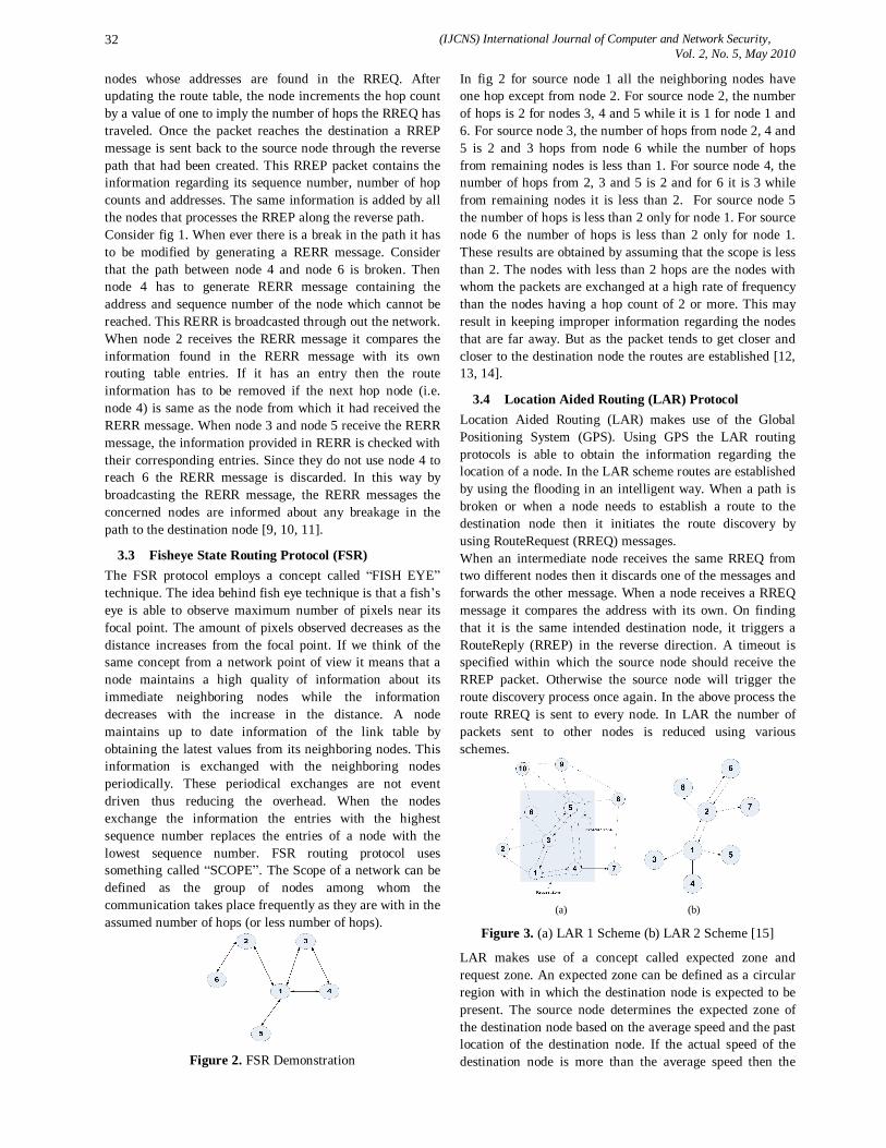
(IJCNS) International Journal of Computer and Network Security, Vol. 2, No. 5, May 2010
32
nodes whose addresses are found in the RREQ. After updating the route table, the node increments the hop count by a value of one to imply the number of hops the RREQ has traveled. Once the packet reaches the destination a RREP message is sent back to the source node through the reverse path that had been created. This RREP packet contains the information regarding its sequence number, number of hop counts and addresses. The same information is added by all the nodes that processes the RREP along the reverse path. Consider fig 1. When ever there is a break in the path it has to be modified by generating a RERR message. Consider that the path between node 4 and node 6 is broken. Then node 4 has to generate RERR message containing the address and sequence number of the node which cannot be reached. This RERR is broadcasted through out the network. When node 2 receives the RERR message it compares the information found in the RERR message with its own routing table entries. If it has an entry then the route information has to be removed if the next hop node (i.e. node 4) is same as the node from which it had received the RERR message. When node 3 and node 5 receive the RERR message, the information provided in RERR is checked with their corresponding entries. Since they do not use node 4 to reach 6 the RERR message is discarded. In this way by broadcasting the RERR message, the RERR messages the concerned nodes are informed about any breakage in the path to the destination node [9, 10, 11].
3.3 Fisheye State Routing Protocol (FSR) The FSR protocol employs a concept called “FISH EYE” technique. The idea behind fish eye technique is that a fish’s eye is able to observe maximum number of pixels near its focal point. The amount of pixels observed decreases as the distance increases from the focal point. If we think of the same concept from a network point of view it means that a node maintains a high quality of information about its immediate neighboring nodes while the information decreases with the increase in the distance. A node maintains up to date information of the link table by obtaining the latest values from its neighboring nodes. This information is exchanged with the neighboring nodes periodically. These periodical exchanges are not event driven thus reducing the overhead. When the nodes exchange the information the entries with the highest sequence number replaces the entries of a node with the lowest sequence number. FSR routing protocol uses something called “SCOPE”. The Scope of a network can be defined as the group of nodes among whom the communication takes place frequently as they are with in the assumed number of hops (or less number of hops).
Figure 2. FSR Demonstration
In fig 2 for source node 1 all the neighboring nodes have one hop except from node 2. For source node 2, the number of hops is 2 for nodes 3, 4 and 5 while it is 1 for node 1 and 6. For source node 3, the number of hops from node 2, 4 and 5 is 2 and 3 hops from node 6 while the number of hops from remaining nodes is less than 1. For source node 4, the number of hops from 2, 3 and 5 is 2 and for 6 it is 3 while from remaining nodes it is less than 2. For source node 5 the number of hops is less than 2 only for node 1. For source node 6 the number of hops is less than 2 only for node 1. These results are obtained by assuming that the scope is less than 2. The nodes with less than 2 hops are the nodes with whom the packets are exchanged at a high rate of frequency than the nodes having a hop count of 2 or more. This may result in keeping improper information regarding the nodes that are far away. But as the packet tends to get closer and closer to the destination node the routes are established [12, 13, 14].
3.4 Location Aided Routing (LAR) Protocol Location Aided Routing (LAR) makes use of the Global Positioning System (GPS). Using GPS the LAR routing protocols is able to obtain the information regarding the location of a node. In the LAR scheme routes are established by using the flooding in an intelligent way. When a path is broken or when a node needs to establish a route to the destination node then it initiates the route discovery by using RouteRequest (RREQ) messages. When an intermediate node receives the same RREQ from two different nodes then it discards one of the messages and forwards the other message. When a node receives a RREQ message it compares the address with its own. On finding that it is the same intended destination node, it triggers a RouteReply (RREP) in the reverse direction. A timeout is specified within which the source node should receive the RREP packet. Otherwise the source node will trigger the route discovery process once again. In the above process the route RREQ is sent to every node. In LAR the number of packets sent to other nodes is reduced using various schemes.
(a) (b)
Figure 3. (a) LAR 1 Scheme (b) LAR 2 Scheme [15]
LAR makes use of a concept called expected zone and request zone. An expected zone can be defined as a circular region with in which the destination node is expected to be present. The source node determines the expected zone of the destination node based on the average speed and the past location of the destination node. If the actual speed of the destination node is more than the average speed then the
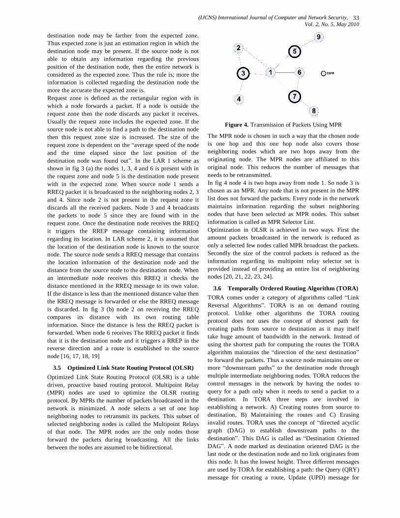
(IJCNS) International Journal of Computer and Network Security, Vol. 2, No. 5, May 2010
33
destination node may be farther from the expected zone. Thus expected zone is just an estimation region in which the destination node may be present. If the source node is not able to obtain any information regarding the previous position of the destination node, then the entire network is considered as the expected zone. Thus the rule is; more the information is collected regarding the destination node the more the accurate the expected zone is. Request zone is defined as the rectangular region with in which a node forwards a packet. If a node is outside the request zone then the node discards any packet it receives. Usually the request zone includes the expected zone. If the source node is not able to find a path to the destination node then this request zone size is increased. The size of the request zone is dependent on the “average speed of the node and the time elapsed since the last position of the destination node was found out”. In the LAR 1 scheme as shown in fig 3 (a) the nodes 1, 3, 4 and 6 is present with in the request zone and node 5 is the destination node present with in the expected zone. When source node 1 sends a RREQ packet it is broadcasted to the neighboring nodes 2, 3 and 4. Since node 2 is not present in the request zone it discards all the received packets. Node 3 and 4 broadcasts the packets to node 5 since they are found with in the request zone. Once the destination node receives the RREQ it triggers the RREP message containing information regarding its location. In LAR scheme 2, it is assumed that the location of the destination node is known to the source node. The source node sends a RREQ message that contains the location information of the destination node and the distance from the source node to the destination node. When an intermediate node receives this RREQ it checks the distance mentioned in the RREQ message to its own value. If the distance is less than the mentioned distance value then the RREQ message is forwarded or else the RREQ message is discarded. In fig 3 (b) node 2 on receiving the RREQ compares its distance with its own routing table information. Since the distance is less the RREQ packet is forwarded. When node 6 receives The RREQ packet it finds that it is the destination node and it triggers a RREP in the reverse direction and a route is established to the source node [16, 17, 18, 19]
3.5 Optimized Link State Routing Protocol (OLSR) Optimized Link State Routing Protocol (OLSR) is a table driven, proactive based routing protocol. Multipoint Relay (MPR) nodes are used to optimize the OLSR routing protocol. By MPRs the number of packets broadcasted in the network is minimized. A node selects a set of one hop neighboring nodes to retransmit its packets. This subset of selected neighboring nodes is called the Multipoint Relays of that node. The MPR nodes are the only nodes those forward the packets during broadcasting. All the links between the nodes are assumed to be bidirectional.
Figure 4. Transmission of Packets Using MPR
The MPR node is chosen in such a way that the chosen node is one hop and this one hop node also covers those neighboring nodes which are two hops away from the originating node. The MPR nodes are affiliated to this original node. This reduces the number of messages that needs to be retransmitted. In fig 4 node 4 is two hops away from node 1. So node 3 is chosen as an MPR. Any node that is not present in the MPR list does not forward the packets. Every node in the network maintains information regarding the subset neighboring nodes that have been selected as MPR nodes. This subset information is called as MPR Selector List. Optimization in OLSR is achieved in two ways. First the amount packets broadcasted in the network is reduced as only a selected few nodes called MPR broadcast the packets. Secondly the size of the control packets is reduced as the information regarding its multipoint relay selector set is provided instead of providing an entire list of neighboring nodes [20, 21, 22, 23, 24].
3.6 Temporally Ordered Routing Algorithm (TORA) TORA comes under a category of algorithms called “Link Reversal Algorithms”. TORA is an on demand routing protocol. Unlike other algorithms the TORA routing protocol does not uses the concept of shortest path for creating paths from source to destination as it may itself take huge amount of bandwidth in the network. Instead of using the shortest path for computing the routes the TORA algorithm maintains the “direction of the next destination” to forward the packets. Thus a source node maintains one or more “downstream paths” to the destination node through multiple intermediate neighboring nodes. TORA reduces the control messages in the network by having the nodes to query for a path only when it needs to send a packet to a destination. In TORA three steps are involved in establishing a network. A) Creating routes from source to destination, B) Maintaining the routes and C) Erasing invalid routes. TORA uses the concept of “directed acyclic graph (DAG) to establish downstream paths to the destination”. This DAG is called as “Destination Oriented DAG”. A node marked as destination oriented DAG is the last node or the destination node and no link originates from this node. It has the lowest height. Three different messages are used by TORA for establishing a path: the Query (QRY) message for creating a route, Update (UPD) message for

(IJCNS) International Journal of Computer and Network Security, Vol. 2, No. 5, May 2010
34
creating and maintaining routes and Clear (CLR) message for erasing a route. Each of the nodes is associated with a height in the network
(a) (b)
Figure 5. Directed Path in TORA
. A link is established between the nodes based on the height. The establishment of the route from source to destination is based on the DAG mechanism thus ensuring that all the routes are loop free. Packets move from the source node having the highest height to the destination node with the lowest height. It’s the same top to down approach. When there is no directed link from source to destination the source node trigger the QRY packet. The source node (node 1) broadcasts the QRY packet across all the nodes in the network. This QRY packet is forwarded by all the intermediate nodes which may contain a path to the destination. Consider fig 5(a). When the QRY packet reaches the destination node (node 9) then the destination node replies with a UPD message. Each node receiving this UPD message will set the value of the height to a value greater than the height of the node from which it had received. This results in the creation of the directed link from the source to the destination. This is the concept involved in the link reversal algorithm. This enables to establish a number of multiple routes from the source to destination. Assume that the path between node 5 and node 6 is broken (fig 5(b)). Then node 6 generates an UPD message with a new height value with in a given “defined time”. Node 3 reverses its link on receiving the UPD message. This reverse link indicates that the path to destination through that directed link is not available. If there is a break between node 1 and node 3 then it results in partition of the network where the resulting invalid routes are erased using the CLR message [25, 26, 27].
3.7 Community Based Mobility Model A new social network based model called Community Mobility Model was proposed by [29]. This mobility model can be used to model humans moving in groups or groups of humans which are clustered together. The authors of the community model have evaluated their model by using the real time synthetic mobility traces provided by the Inter Research Laboratory, Cambridge. The Community Model can be conceptualized as below:
Figure 6. Steps Involved in the Establishment of the
Community Mobility Model [29]
The first step in establishing a community model is using the “Social network as input” to the community mobility model. It involves two ways i.e. “modeling of social relationships” and “detection of community structures”. Modeling of social relationship can be represented as a weighted graph matrix. If any of the elements in the matrix is greater than the specified threshold value then that element in the graph is set to 1 and if it is less than the threshold value then it is set to 0. A value of 1 represents strong social interaction between the groups and a value of 0 represents no interaction. The concept of 1 and 0 is used to emphasize the relation between any two members of a group or any individuals of the group. The next step is to conceptualize the interaction between groups of a social community network. The authors of the community model have implemented this aspect by considering an algorithm provided by [28]. Groups communicate with each other through “inter community edges” and this concept is called as “betweeness of edges”. Once the connection between the individuals in the communities and the interaction between the communities itself is established then the next step is the placement of the communities in a square location on a grid. This can be represented by Spq i.e. “a square in position of p, q”. The next step is the dynamics of the mobile host. For mobility, a host from each group or community is selected. For each of the host the first goal is randomly chosen inside the square Spq. Here goal represents the mobility position. The next goal is selected by the “social attractivity”. Each host will have a certain attraction for another host representing another square location. When a host is attracted to another host then the community moves from the present square location to the square location of another host to which the present host is attracted. Finally, the mobile host needs to be associated with the mobility dynamics.
3.8 Semi-Markov Smooth (SMS) Mobility Model Semi Markov Smooth (SMS) mobility model obeys the physical law of smooth mobility. It has three phases a) speed up phase b) middle smooth phase and c) slow down phase. In the speed up phase or α phase the object is accelerated until it reaches an acceptable speed. The speed up phase time interval is given by [ ] [ ]ttttt ∆++= αα 000 , where t0

(IJCNS) International Journal of Computer and Network Security, Vol. 2, No. 5, May 2010
35
is the initial time and tα is the alpha phase time. Once the object is moving at an acceptable normal speed then it has to maintain this speed for some time. The middle smooth phase or β phase is represented by [ ]ttttt ∆+= βααβα ,, where β is uniformly distributed
over [βmin, βmax]. As we know that every moving object at some point of time has to slow down and eventually stop. The node reaches γ phase or slow down phase. The node remains in this phase for a random period of time before the speed reaches to Vγ = 0. Distance between any two points is treated as the Euclidian distance. Trace length is the actual length traveled by a node during one movement without any change in that direction. Distance evolution is the way the traveling of a node is observed. If the speed of a node increases continuously then the α phase and β phase of the trace length is equivalent to the distance evolution. This results in a smooth trace. When the speed of the node decreases in the γ phase it results in a sharp curve. SMS mobility model can also be considered as a group mobility model. In this scenario a node is selected as a leader. This group leader selects a speed and direction which the other nodes do follow. The velocity of a group member m at its nth step is given by
( ) max1 VUVV Leadern
mn ∆⋅⋅−+= ρ
( )max1 φρφφ ∆⋅⋅−+= ULeadern
mn
Where U is a random variable, ∆Vmax is the maximum speed and φmax is the difference in the direction of the common node and the leader node in one step [30, 31].
3.9 Energy Model The Energy Consumption model considered in this paper is based on a study done in [32, 33]. The amount of energy spent in transmitting and receiving the packets is calculated by using the following equations: Energytx = (330*PacketSize)/2*106 Energyrx = (230*PacketSize)/2*106 where packet size is specified in bits. Average Energy Consumed is defined as
desNumberofNoodesumedbyallNEnergyConsPercentage∑
4. Simulation Environment Simulations are performed using Network Simulator NS-2 [34]. The simulated values of the radio network interface card are based on the 914MHz Lucent WaveLan direct sequence spread spectrum radio model. This model has a bit rate of 2 Mbps and a radio transmission range of 250m. The IEEE 802.11 distributed coordinated function with CSMA/CA is used as the underlying MAC protocol. Interface Queue (IFQ) value of 70 is used to queue the routing and data packets. Following metrics have been selected for evaluating the
mobility models: Packet Delivery Ratio: It is defined as
∑∑
Packets DataSent ofNumber
Packets Data Received ofNumber
Average Network Delay: It is defined as ( )
Pairs Connection ofNumber Total@sourcesent packet Time@dest arrivepacket Time∑ −
Throughput of the network: Throughput is defined as
Nodes ofNumber TotalonTransmissi Data of sThroughput Node∑
Routing Overhead: It is defined as ( ) ( )[ ]
sim
fwdSizepkt sentsizepkt
ΔT
Control MAC Control MAC∑ +
Table 1: Simulation Parameters Simulator NS2
Routing Protocols AOMDV, DYMO, FSR, LAR, OLSR and TORA
Mobility Model Community Mobility Model and SMS Mobility Model
Simulation Time (sec)
900
Pause Time (sec) 10
Simulation Area (m)
1000 x 1000
Number of Nodes 10, 20, 30, 40, 50
Transmission Range
250 m
Maximum Speed (m/s)
5, 10, 15, 20, 25
Traffic Rate (pkts/sec)
5, 10, 15, 20, 25
Data Payload (Bytes)
512
5. Result Analysis All the simulations scenarios are averaged for 5 different seeds while running independently. We have considered the effect of mobility speed, node density and traffic load on the performance of these routing protocols using Community based mobility model and SMS mobility model. Effect of Mobility Speed
5.1 Effect of Mobility Speed Both the Mobility speed and the type of Mobility model play a vital role in determining the performance of routing protocols. The mobility speed is varied from 5 m/s to 25 m/s in steps of 5. The routing protocols LAR, AOMDV and TORA are compared using the Community Based Mobility Model and the routing protocols OLSR, DYMO and FSR are compared using SMS mobility model. In this paper scheme one implementation of route establishment is employed in LAR routing protocol. The
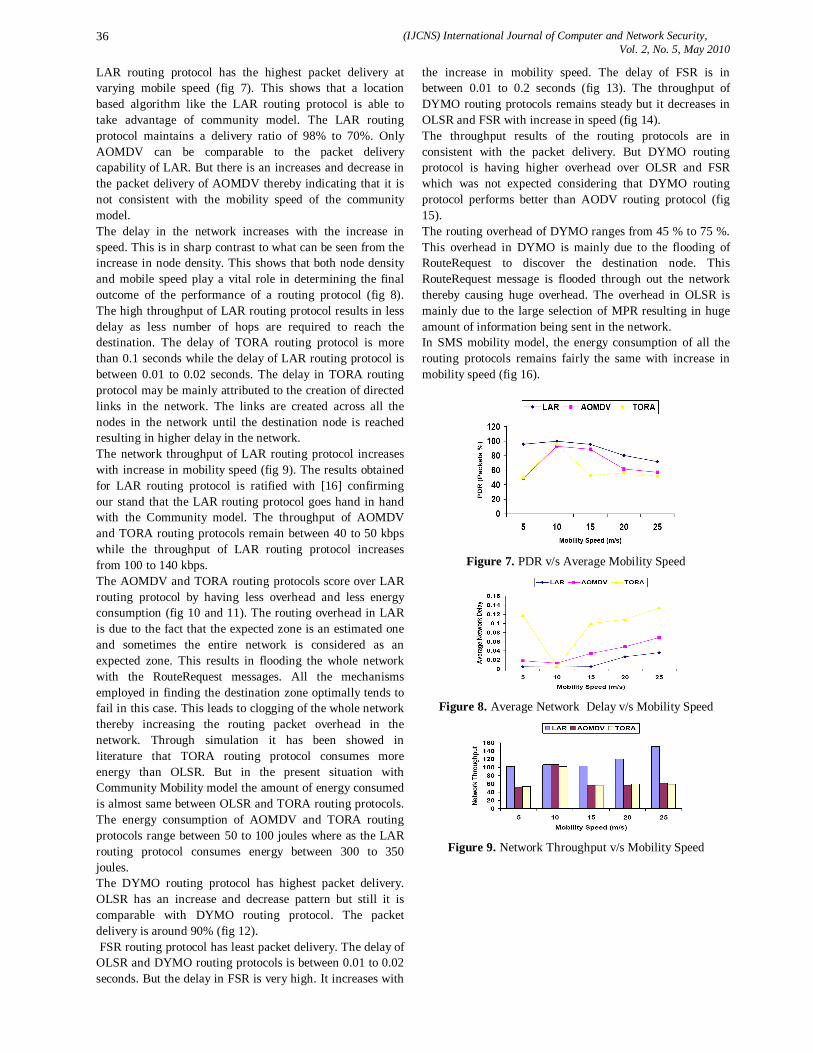
(IJCNS) International Journal of Computer and Network Security, Vol. 2, No. 5, May 2010
36
LAR routing protocol has the highest packet delivery at varying mobile speed (fig 7). This shows that a location based algorithm like the LAR routing protocol is able to take advantage of community model. The LAR routing protocol maintains a delivery ratio of 98% to 70%. Only AOMDV can be comparable to the packet delivery capability of LAR. But there is an increases and decrease in the packet delivery of AOMDV thereby indicating that it is not consistent with the mobility speed of the community model. The delay in the network increases with the increase in speed. This is in sharp contrast to what can be seen from the increase in node density. This shows that both node density and mobile speed play a vital role in determining the final outcome of the performance of a routing protocol (fig 8). The high throughput of LAR routing protocol results in less delay as less number of hops are required to reach the destination. The delay of TORA routing protocol is more than 0.1 seconds while the delay of LAR routing protocol is between 0.01 to 0.02 seconds. The delay in TORA routing protocol may be mainly attributed to the creation of directed links in the network. The links are created across all the nodes in the network until the destination node is reached resulting in higher delay in the network. The network throughput of LAR routing protocol increases with increase in mobility speed (fig 9). The results obtained for LAR routing protocol is ratified with [16] confirming our stand that the LAR routing protocol goes hand in hand with the Community model. The throughput of AOMDV and TORA routing protocols remain between 40 to 50 kbps while the throughput of LAR routing protocol increases from 100 to 140 kbps. The AOMDV and TORA routing protocols score over LAR routing protocol by having less overhead and less energy consumption (fig 10 and 11). The routing overhead in LAR is due to the fact that the expected zone is an estimated one and sometimes the entire network is considered as an expected zone. This results in flooding the whole network with the RouteRequest messages. All the mechanisms employed in finding the destination zone optimally tends to fail in this case. This leads to clogging of the whole network thereby increasing the routing packet overhead in the network. Through simulation it has been showed in literature that TORA routing protocol consumes more energy than OLSR. But in the present situation with Community Mobility model the amount of energy consumed is almost same between OLSR and TORA routing protocols. The energy consumption of AOMDV and TORA routing protocols range between 50 to 100 joules where as the LAR routing protocol consumes energy between 300 to 350 joules. The DYMO routing protocol has highest packet delivery. OLSR has an increase and decrease pattern but still it is comparable with DYMO routing protocol. The packet delivery is around 90% (fig 12). FSR routing protocol has least packet delivery. The delay of OLSR and DYMO routing protocols is between 0.01 to 0.02 seconds. But the delay in FSR is very high. It increases with
the increase in mobility speed. The delay of FSR is in between 0.01 to 0.2 seconds (fig 13). The throughput of DYMO routing protocols remains steady but it decreases in OLSR and FSR with increase in speed (fig 14). The throughput results of the routing protocols are in consistent with the packet delivery. But DYMO routing protocol is having higher overhead over OLSR and FSR which was not expected considering that DYMO routing protocol performs better than AODV routing protocol (fig 15). The routing overhead of DYMO ranges from 45 % to 75 %. This overhead in DYMO is mainly due to the flooding of RouteRequest to discover the destination node. This RouteRequest message is flooded through out the network thereby causing huge overhead. The overhead in OLSR is mainly due to the large selection of MPR resulting in huge amount of information being sent in the network. In SMS mobility model, the energy consumption of all the routing protocols remains fairly the same with increase in mobility speed (fig 16).
Figure 7. PDR v/s Average Mobility Speed
Figure 8. Average Network Delay v/s Mobility Speed
Figure 9. Network Throughput v/s Mobility Speed

(IJCNS) International Journal of Computer and Network Security, Vol. 2, No. 5, May 2010
37
Figure 10. Routing Overhead v/s Mobility Speed
Figure 11. Average Energy Consumed v/s Mobility
Speed
Figure 12. PDR v/s Mobility Speed
Figure 13. Average Network Delay v/s Mobility Speed
Figure 14. Network Throughput v/s Mobility Speed
Figure 15. Routing Overhead v/s Mobility Speed
Figure 16. Average Energy Consumed v/s Mobility
Speed
5.2 Effect of Node Density The number of nodes is varied from 10 to 50 in steps of 10. Our goal is not to find the optimum number of nodes for these routing protocols but to see how these routing protocols fare against different node densities. Higher node density enables us to analyze whether these routing protocols are able to take the inherent advantages of a community model especially the LAR routing protocol. The routing protocols LAR, AOMDV and TORA are mapped against number of nodes using Community Based Mobility Model. At higher node density the connectivity between nodes is significantly better resulting in better packet delivery. When the number of nodes is less the LAR routing protocol has better packet delivery ratio. But when the number of nodes is increased to more than 30 then all the routing protocols converge to the same level. At higher node density all the routing protocols are able to provide nearly 100% packet delivery (fig 17). The TORA routing protocol has the highest delay at lower node density (fig 18). But as the node increases delay decreases among all the routing protocols. AOMDV has the least delay when compared to LAR and TORA routing protocols. The delay in AOMDV is less due to the availability of alternate routes thus avoiding the necessity of sending the RouteRequest packets again and again. It can be noticed that the throughput of all the protocols increases with the increase in node density (fig 19). This is due to increase in network connectivity. The routing overhead of LAR routing protocol is astronomically high when compared to AOMDV and TORA routing protocols. This can be attributed to the amount of RouteRequest packet that is flooded through out the network. Even though the LAR routing protocol has various mechanisms to make the flooding of network an intelligent one still the amount of packet needed to discover the destination node in the estimated zone itself results in too much overhead in the network (fig 20). The routing overhead of AOMDV is due to the additional RouteRequest that are needed to maintain multiple path in the network. The energy consumption of all the routing protocols increases with the increase in the number of nodes. More energy is consumed by LAR routing protocol (fig 21). The increase in the energy consumption in LAR routing protocol is due to the underlying flooding nature of the routing protocol. Our simulation result sprang a few quite surprises. We were

(IJCNS) International Journal of Computer and Network Security, Vol. 2, No. 5, May 2010
38
expecting TORA to take advantage of its location capabilities when employed under the Community Mobility Model. But here the best all round performer was AOMDV routing protocol. This shows that if were to employ a routing protocol for analyzing realistic mobility models like community models then AOMDV is the well versed routing protocol.
Figure 17. PDR v/s Number of Nodes
Figure 18. Average Network Delay v/s
Number of Nodes
Figure 19. Network Throughput v/s Number
of Nodes
Figure 20. Routing Overhead v/s Number of
Nodes
Figure 21. Average Energy Consumed v/s
Number of Nodes
5.3 Effect of Traffic Load The traffic load is varied from 5 pkts/sec to 25 pkts/sec in steps of 5. The OLSR, DYMO and FSR routing protocols are analyzed using SMS mobility model with varying traffic load. The packet delivery of OLSR and DYMO remains close to 100% up to 10 pkts/sec (fig 22). With the increase in traffic load the packet delivery of all the routing protocols tend to decrease. The DYMO Routing protocol is able to cope with the congestion in the network better than OLSR and FSR routing protocols. The delay in FSR is the worst when compared to OLSR and DYMO. There is an astronomical increase in delay for FSR routing protocol starting from 5 pkts/sec and for OLSR the delay increases after 10 pkts/sec. The DYMO routing protocol has less delay when compared to other two routing protocols (fig 23). The delay in DYMO routing protocol increases after 15 pkts/sec. The delay varies from 0.1 seconds to 0.4 seconds. Even though DYMO has less delay and more packet delivery to fails to maintain the momentum for network throughput (fig 24). Surprisingly both OLSR and FSR routing protocols score over DYMO in network throughput. The throughput of all the routing protocols increases with the increase in the traffic load. The routing overhead of DYMO increases with increase in traffic load while the routing overhead of OLSR and FSR decreases with increase in traffic load. FSR is having less routing overhead. This factor can be attributed to the unique feature in FSR where it maintains the information of its immediate neighboring nodes thereby it is able to find the destination node with minimum number of hops (fig 25). DYMO protocol’s routing overhead increases up to 15 pkts/sec and maintain a steady state after that indicating that the network is saturated. The routing overhead of OLSR and FSR decreases with the increase in traffic load. The routing overhead of FSR decreases from 10% to 4% with the increase in traffic load. Both OLSR and FSR have high energy consumption. Above 10 pkts/sec the energy consumption of OLSR increases at a very high rate. But the energy consumption of FSR routing is more than 300 joules starting from 5 pkts/sec (fig 26). DYMO routing protocol maintains steady energy consumption between 150 to 200 joules. For SMS mobility model if high packet delivery, less delay and less energy consumption are the criterion to employ a routing protocol then the routing protocol of choice should

(IJCNS) International Journal of Computer and Network Security, Vol. 2, No. 5, May 2010
39
be the DYMO routing protocol.
Figure 22. PDR v/s Traffic Load
Figure 23. Average Network Delay v/s Traffic Load
Figure 24. Network Throughput v/s Traffic Load
Figure 25. Routing Overhead v/s Traffic Load
Figure 26. Average Energy Consumed v/s Traffic
Load
6 Conclusion In this paper we have evaluated six routing protocols over two realistic mobility models. We have conducted these experiments in best possible scenarios conductive for an ad hoc network to understand the performance of these routing protocols over different mobility model. The LAR routing protocol is the protocol of choice for a community model moving at high speed. We came across few surprises like
AOMDV performing better than the LAR routing protocol at higher node density for a Community Based Mobility Model. The DYMO routing protocol outperforms both OLSR and FSR with varying mobility speed and traffic load. At the end of the day the type of routing protocols that needs to be deployed depends on the situation in hand in addition to the various parameters given in our paper.
Acknowledgments The first author of this paper would like to acknowledge the help of Tracy Camp, Wenye Wang, Mirco Musolesi in this work.
References [1] A.K.Dwivedi et al.,”Performance of Routing Protocols
for Mobile Adhoc and Wireless Sensor Networks: A Comparative Study”, International Journal of Recent Trends in Engineering, Vol 2, No. 4, November 2009.
[2] Nicholas Cooper and Natarajan Meganathan,”Impact of Mobility Models on Multi Path Routing in Mobile Ad Hoc Networks”, International Journal of Computer Networks and Communications (IJCNC), Vol 2, No 1, January 2010.
[3] Anders Nilsson,”Performance Analysis of Traffic Load and Node Density in Ad hoc Networks”, In Proceedings of the 5th European Wireless Conference (EW2004) Mobile and Wireless Systems, Barcelona, Spain, Feb 24-27, 2004.
[4] M.I.M Saad et al,“Performance Analysis of Random Based Mobility Models in MANET Routing Protocol”, European Journal of Scientific Research, Vol 32, No. 4, pp 444-454.
[5] Biao Zhou, Kaixin Xu and Mario Gerla,”Group and Swarm Mobility Models for Ad hoc Network Scenarios Using Virtual Tracks”, IEEE Military Communications Conference (MILCOM’04), Moneterey, California, USA, Oct 31-Nov 3, 2004.
[6] Sven Jaap, Marc Bechler and Lars Worf,”Evaluation of Routing Protocols for Vehicular Ad hoc Networks in City Traffic Scenarios”, In Proceedings of the 5th International Conference o Intelligent Transportation Systems Telecommunications (ITST), Brest, France, June 2005.
[7] Mahesh K. Marina and Samir R.Das, “ On-Demand Multipath Distance Vector Routing in Ad-hoc Networks”, In proceedings of the IEEE International Conference on Network Protocols, 2001 pp 14-23.
[8] M.Caleffi, G.Ferraiuolo and L.Pauro, “On Reliability of Dynamic Addressing Protocols in Mobile Ad hoc Networks”, Proceedings of WRECOM’07, Wireless Rural and Emergency Communications Conference, Roma, Italy, October 2007.
[9] Ian D Chakeres and Charles E Perkins,”Dynamic Manet On Demand Routing Protocol”, IETF Internet Draft, draft-ietf-manet-dymo-12.txt, February 2008.
[10] Rolf Ehrenreich Thorup,”Implementing and Evaluating the DYMO Routing Protocol”, Master’s Thesis, Department of Comptuer Science, University of Aarhus, Denmark.
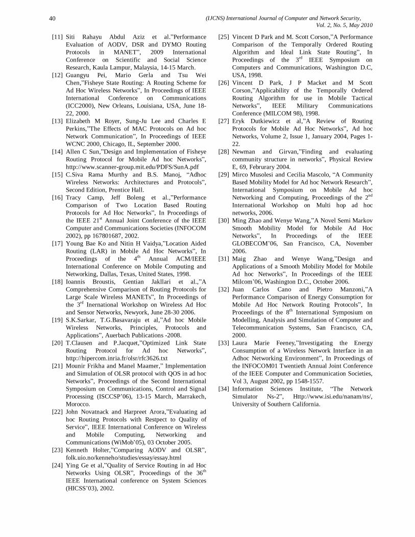
(IJCNS) International Journal of Computer and Network Security, Vol. 2, No. 5, May 2010
40
[11] Siti Rahayu Abdul Aziz et al.”Performance Evaluation of AODV, DSR and DYMO Routing Protocols in MANET”, 2009 International Conference on Scientific and Social Science Research, Kaula Lampur, Malaysia, 14-15 March.
[12] Guangyu Pei, Mario Gerla and Tsu Wei Chen,”Fisheye State Routing: A Routing Scheme for Ad Hoc Wireless Networks”, In Proceedings of IEEE International Conference on Communications (ICC2000), New Orleans, Louisiana, USA, June 18-22, 2000.
[13] Elizabeth M Royer, Sung-Ju Lee and Charles E Perkins,”The Effects of MAC Protocols on Ad hoc Network Communication”, In Proceedings of IEEE WCNC 2000, Chicago, IL, September 2000.
[14] Allen C Sun,”Design and Implementation of Fisheye Routing Protocol for Mobile Ad hoc Networks”, http://www.scanner-group.mit.edu/PDFS/SunA.pdf
[15] C.Siva Rama Murthy and B.S. Manoj, “Adhoc Wireless Networks: Architectures and Protocols”, Second Edition, Prentice Hall.
[16] Tracy Camp, Jeff Boleng et al.,”Performance Comparison of Two Location Based Routing Protocols for Ad Hoc Networks”, In Proceedings of the IEEE 21st Annual Joint Conference of the IEEE Computer and Communications Societies (INFOCOM 2002), pp 167801687, 2002.
[17] Young Bae Ko and Nitin H Vaidya,”Location Aided Routing (LAR) in Mobile Ad Hoc Networks”, In Proceedings of the 4th Annual ACM/IEEE International Conference on Mobile Computing and Networking, Dallas, Texas, United States, 1998.
[18] Ioannis Broustis, Gentian Jakllari et al.,”A Comprehensive Comparison of Routing Protocols for Large Scale Wireless MANETs”, In Proceedings of the 3rd Inernational Workshop on Wireless Ad Hoc and Sensor Networks, Newyork, June 28-30 2006.
[19] S.K.Sarkar, T.G.Basavaraju et al,”Ad hoc Mobile Wireless Networks, Principles, Protocols and Applications”, Auerbach Publications -2008.
[20] T.Clausen and P.Jacquet,”Optimized Link State Routing Protocol for Ad hoc Networks”, http://hipercom.inria.fr/olsr/rfc3626.txt
[21] Mounir Frikha and Manel Maamer,” Implementation and Simulation of OLSR protocol with QOS in ad hoc Networks”, Proceedings of the Second International Symposium on Communications, Control and Signal Processing (ISCCSP’06), 13-15 March, Marrakech, Morocco.
[22] John Novatnack and Harpreet Arora,”Evaluating ad hoc Routing Protocols with Restpect to Quality of Service”, IEEE International Conference on Wireless and Mobile Computing, Networking and Communications (WiMob’05), 03 October 2005.
[23] Kenneth Holter,”Comparing AODV and OLSR”, folk.uio.no/kenneho/studies/essay/essay.html
[24] Ying Ge et al,”Quality of Service Routing in ad Hoc Networks Using OLSR”, Proceedings of the 36th IEEE International conference on System Sciences (HICSS’03), 2002.
[25] Vincent D Park and M. Scott Corson,”A Performance Comparison of the Temporally Ordered Routing Algorithm and Ideal Link State Routing”, In Proceedings of the 3rd IEEE Symposium on Computers and Communications, Washington D.C, USA, 1998.
[26] Vincent D Park, J P Macket and M Scott Corson,”Applicability of the Temporally Ordered Routing Algorithm for use in Mobile Tactical Networks”, IEEE Military Communications Conference (MILCOM 98), 1998.
[27] Eryk Dutkiewicz et al,”A Review of Routing Protocols for Mobile Ad Hoc Networks”, Ad hoc Networks, Volume 2, Issue 1, January 2004, Pages 1-22.
[28] Newman and Girvan,”Finding and evaluating community structure in networks”, Physical Review E, 69, Februrary 2004.
[29] Mirco Musolesi and Cecilia Mascolo, “A Community Based Mobility Model for Ad hoc Network Research”, International Symposium on Mobile Ad hoc Networking and Computing, Proceedings of the 2nd International Workshop on Multi hop ad hoc networks, 2006.
[30] Ming Zhao and Wenye Wang,”A Novel Semi Markov Smooth Mobility Model for Mobile Ad Hoc Networks”, In Proceedings of the IEEE GLOBECOM’06, San Francisco, CA, November 2006.
[31] Maig Zhao and Wenye Wang,”Design and Applications of a Smooth Mobility Model for Mobile Ad hoc Networks”, In Proceedings of the IEEE Milcom’06, Washington D.C., October 2006.
[32] Juan Carlos Cano and Pietro Manzoni,”A Performance Comparison of Energy Consumption for Mobile Ad Hoc Network Routing Protocols”, In Proceedings of the 8th International Symposium on Modelling, Analysis and Simulation of Computer and Telecommunication Systems, San Francisco, CA, 2000.
[33] Laura Marie Feeney,”Investigating the Energy Consumption of a Wireless Network Interface in an Adhoc Networking Environment”, In Proceedings of the INFOCOM01 Twentieth Annual Joint Conference of the IEEE Computer and Communication Societies, Vol 3, August 2002, pp 1548-1557.
[34] Information Sciences Institute, “The Network Simulator Ns-2”, Http://www.isi.edu/nanam/ns/, University of Southern California.
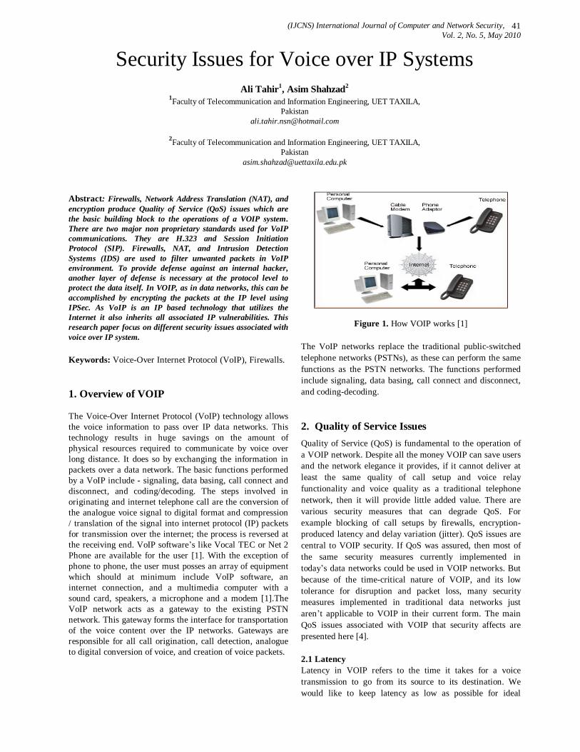
(IJCNS) International Journal of Computer and Network Security, Vol. 2, No. 5, May 2010
41
Security Issues for Voice over IP Systems
Ali Tahir1, Asim Shahzad2 1Faculty of Telecommunication and Information Engineering, UET TAXILA,
Pakistan [email protected]
2Faculty of Telecommunication and Information Engineering, UET TAXILA,
Pakistan [email protected]
Abstract: Firewalls, Network Address Translation (NAT), and encryption produce Quality of Service (QoS) issues which are the basic building block to the operations of a VOIP system. There are two major non proprietary standards used for VoIP communications. They are H.323 and Session Initiation Protocol (SIP). Firewalls, NAT, and Intrusion Detection Systems (IDS) are used to filter unwanted packets in VoIP environment. To provide defense against an internal hacker, another layer of defense is necessary at the protocol level to protect the data itself. In VOIP, as in data networks, this can be accomplished by encrypting the packets at the IP level using IPSec. As VoIP is an IP based technology that utilizes the Internet it also inherits all associated IP vulnerabilities. This research paper focus on different security issues associated with voice over IP system. Keywords: Voice-Over Internet Protocol (VoIP), Firewalls.
1. Overview of VOIP
The Voice-Over Internet Protocol (VoIP) technology allows the voice information to pass over IP data networks. This technology results in huge savings on the amount of physical resources required to communicate by voice over long distance. It does so by exchanging the information in packets over a data network. The basic functions performed by a VoIP include - signaling, data basing, call connect and disconnect, and coding/decoding. The steps involved in originating and internet telephone call are the conversion of the analogue voice signal to digital format and compression / translation of the signal into internet protocol (IP) packets for transmission over the internet; the process is reversed at the receiving end. VoIP software’s like Vocal TEC or Net 2 Phone are available for the user [1]. With the exception of phone to phone, the user must posses an array of equipment which should at minimum include VoIP software, an internet connection, and a multimedia computer with a sound card, speakers, a microphone and a modem [1].The VoIP network acts as a gateway to the existing PSTN network. This gateway forms the interface for transportation of the voice content over the IP networks. Gateways are responsible for all call origination, call detection, analogue to digital conversion of voice, and creation of voice packets.
Figure 1. How VOIP works [1] The VoIP networks replace the traditional public-switched telephone networks (PSTNs), as these can perform the same functions as the PSTN networks. The functions performed include signaling, data basing, call connect and disconnect, and coding-decoding.
2. Quality of Service Issues Quality of Service (QoS) is fundamental to the operation of a VOIP network. Despite all the money VOIP can save users and the network elegance it provides, if it cannot deliver at least the same quality of call setup and voice relay functionality and voice quality as a traditional telephone network, then it will provide little added value. There are various security measures that can degrade QoS. For example blocking of call setups by firewalls, encryption-produced latency and delay variation (jitter). QoS issues are central to VOIP security. If QoS was assured, then most of the same security measures currently implemented in today’s data networks could be used in VOIP networks. But because of the time-critical nature of VOIP, and its low tolerance for disruption and packet loss, many security measures implemented in traditional data networks just aren’t applicable to VOIP in their current form. The main QoS issues associated with VOIP that security affects are presented here [4]. 2.1 Latency Latency in VOIP refers to the time it takes for a voice transmission to go from its source to its destination. We would like to keep latency as low as possible for ideal

(IJCNS) International Journal of Computer and Network Security, Vol. 2, No. 5, May 2010
42
systems but there are practical lower bounds on the delay of VOIP. The ITU-T Recommendation G.114 establishes a number of time constraints on one-way latency. The upper bound is 150 ms in [2] for one-way traffic experienced in domestic calls across PSTN lines in the continental United States. For international calls, a delay of up to 400 ms was deemed tolerable, but since most of the added time is spent routing and moving the data over long distances, we consider here only the domestic case and assume our solutions are upwards compatible in the international realm. VOIP calls must achieve the 150 ms bound to successfully emulate the QoS that today’s phones provide. It places a genuine constraint on the amount of security that can be added to a VOIP network. The encoding of voice data can take between 1 and 30 ms and voice data traveling across the North American continent can take upwards of 100 ms although actual travel time is often much faster . Assuming the worst case (100 ms transfer time), 20 –50 ms remain for queuing and security implementations [4].
Figure 2. Sample Latency Budget [4]
Delay is not confined to the endpoints of the system. Each hop along the network introduces a new queuing delay and possibly a processing delay if it is a security checkpoint (i.e. firewall or encryption/decryption point). Also, larger packets tend to cause bandwidth congestion and increased latency. In light of these issues, VOIP tends to work best with small packets on a logically abstracted network to keep latency at a minimum. 2.2 Jitter Jitter refers to non-uniform packet delays. It is often caused by low bandwidth situations in VOIP and can be exceptionally detrimental to the overall QoS. Variations in delays can be more detrimental to QoS than the actual delays themselves. Jitter can cause packets to arrive and be processed out of sequence. RTP, the protocol used to transport voice media, is based on UDP so packets out of order are not reassembled at the protocol level. However, RTP allows applications to do the reordering using the sequence number and timestamp fields. The overhead in
reassembling these packets is non-trivial, especially when dealing with the tight time constraints of VOIP. When jitter is high, packets arrive at their destination in spurts. The general prescription to control jitter at VOIP endpoints is the use of a buffer, but such a buffer has to release its voice packets at least every 150 ms (usually a lot sooner given the transport delay) so the variations in delay must be bounded. The buffer implementation issue is compounded by the uncertainty of whether a missing packet is simply delayed an anomalously long amount of time, or is actually lost. Jitter can also be controlled throughout the VOIP network by using routers, firewalls, and other network elements that support QoS. These elements process and pass along time urgent traffic like VOIP packets sooner than less urgent data packets. Another method for reducing delay variation is to pattern network traffic to diminish jitter by making as efficient use of the bandwidth as possible. This constraint is at odds with some security measures in VOIP. Chief among these is IPSec, whose processing requirements may increase latency, thus limiting effective bandwidth and contributing to jitter. The window of delivery for a VOIP packet is very small, so it follows that the acceptable variation in packet delay is even smaller. Thus, although we are concerned with security, the utmost care must be given to assuring that delays in packet deliveries caused by security devices are kept uniform throughout the traffic stream [4]. 2.3 Packet Loss VOIP is exceptionally intolerant of packet loss. Packet loss can result from excess latency, where a group of packets arrives late and must be discarded in favor of newer ones. It can also be the result of jitter, that is, when a packet arrives after its surrounding packets have been flushed from the buffer, making the received packet useless. Compounding the packet loss problem is VOIP’s reliance on RTP, which uses the unreliable UDP for transport, and thus does not guarantee packet delivery. However, the time constraints do not allow for a reliable protocol such as TCP to be used to deliver media. The good news is that VOIP packets are very small, containing a payload of only 10-50 bytes, which is approximately 12.5-62.5 ms in [4], with most implementations tending toward the shorter range. The loss of such a minuscule amount of speech is not discernable or at least not worthy of complaint for a human VOIP user. The bad news is these packets are usually not lost in isolation. Bandwidth congestion and other such causes of packet loss tend to affect all the packets being delivered around the same time. So although the loss of one packet is fairly inconsequential, probabilistically the loss of one packet means the loss of several packets, which severely degrades the quality of service in a VOIP network. Despite the infeasibility of using a guaranteed delivery protocol such as TCP, there are some remedies for the packet loss problem. One cannot guarantee all packets are delivered, but if bandwidth is available, sending redundant information can probabilistically annul the chance of loss.
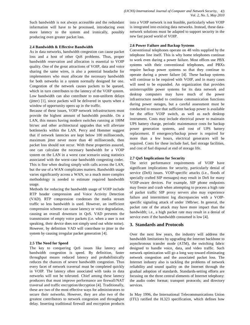
(IJCNS) International Journal of Computer and Network Security, Vol. 2, No. 5, May 2010
43
Such bandwidth is not always accessible and the redundant information will have to be processed, introducing even more latency to the system and ironically, possibly producing even greater packet loss. 2.4 Bandwidth & Effective Bandwidth As in data networks, bandwidth congestion can cause packet loss and a host of other QoS problems. Thus, proper bandwidth reservation and allocation is essential to VOIP quality. One of the great attractions of VOIP, data and voice sharing the same wires, is also a potential headache for implementers who must allocate the necessary bandwidth for both networks in a system normally designed for one. Congestion of the network causes packets to be queued, which in turn contributes to the latency of the VOIP system. Low bandwidth can also contribute to non-uniform delays (jitter) [1], since packets will be delivered in spurts when a window of opportunity opens up in the traffic. Because of these issues, VOIP network infrastructures must provide the highest amount of bandwidth possible. On a LAN, this means having modern switches running at 100M bit/sec and other architectural upgrades that will alleviate bottlenecks within the LAN. Percy and Hommer suggest that if network latencies are kept below 100 milliseconds, maximum jitter never more than 40 milliseconds, then packet loss should not occur. With these properties assured, one can calculate the necessary bandwidth for a VOIP system on the LAN in a worst case scenario using statistics associated with the worst-case bandwidth congesting codec. This is fine when dealing simply with calls across the LAN, but the use of a WAN complicates matters. Bandwidth usage varies significantly across a WAN, so a much more complex methodology is needed to estimate required bandwidth usage. Methods for reducing the bandwidth usage of VOIP include RTP header compression and Voice Activity Detection (VAD). RTP compression condenses the media stream traffic so less bandwidth is used. However, an inefficient compression scheme can cause latency or voice degradation, causing an overall downturn in QoS. VAD prevents the transmission of empty voice packets (i.e. when a user is not speaking, their device does not simply send out white noise). However, by definition VAD will contribute to jitter in the system by causing irregular packet generation [4]. 2.5 The Need for Speed The key to conquering QoS issues like latency and bandwidth congestion is speed. By definition, faster throughput means reduced latency and probabilistically reduces the chances of severe bandwidth congestion. Thus every facet of network traversal must be completed quickly in VOIP. The latency often associated with tasks in data networks will not be tolerated. Chief among these latency producers that must improve performance are firewall/NAT traversal and traffic encryption/decryption [4]. Traditionally, these are two of the most effective ways for administrators to secure their networks. However, they are also two of the greatest contributors to network congestion and throughput delay. Inserting traditional firewall and encryption products
into a VOIP network is not feasible, particularly when VOIP is integrated into existing data networks. Instead, these data-network solutions must be adapted to support security in the new fast paced world of VOIP. 2.6 Power Failure and Backup Systems Conventional telephones operate on 48 volts supplied by the telephone line itself. This is why home telephones continue to work even during a power failure. Most offices use PBX systems with their conventional telephones, and PBXs require backup power systems so that they continue to operate during a power failure [4]. These backup systems will continue to be required with VOIP, and in many cases will need to be expanded. An organization that provides uninterruptible power systems for its data network and desktop computers may have much of the power infrastructure needed to continue communication functions during power outages, but a careful assessment must be conducted to ensure that sufficient backup power is available for the office VOIP switch, as well as each desktop instrument. Costs may include electrical power to maintain UPS battery charge, periodic maintenance costs for backup power generation systems, and cost of UPS battery replacement. If emergency/backup power is required for more than a few hours, electrical generators will be required. Costs for these include fuel, fuel storage facilities, and cost of fuel disposal at end of storage life. 2.7 QoS Implications for Security The strict performance requirements of VOIP have significant implications for security, particularly denial of service (DoS) issues. VOIP-specific attacks (i.e., floods of specially crafted SIP messages) may result in DoS for many VOIP-aware devices. For example, SIP phone endpoints may freeze and crash when attempting to process a high rate of packet traffic SIP proxy servers also may experience failure and intermittent log discrepancies with a VOIP-specific signaling attack of under 1Mb/sec. In general, the packet rate of the attack may have more impact than the bandwidth; i.e., a high packet rate may result in a denial of service even if the bandwidth consumed is low [4].
3. Standards and Protocols
Over the next few years, the industry will address the bandwidth limitations by upgrading the Internet backbone to asynchronous transfer mode (ATM), the switching fabric designed to handle voice, data, and video traffic. Such network optimization will go a long way toward eliminating network congestion and the associated packet loss. The Internet industry also is tackling the problems of network reliability and sound quality on the Internet through the gradual adoption of standards. Standards-setting efforts are focusing on the three central elements of Internet telephony: the audio codec format; transport protocols; and directory services.
In May 1996, the International Telecommunications Union (ITU) ratified the H.323 specification, which defines how

(IJCNS) International Journal of Computer and Network Security, Vol. 2, No. 5, May 2010
44
voice, data, and video traffic will be transported over IP– based local area networks; it also incorporates the T.120 data conferencing standard. The recommendation is based on the real-time protocol/real-time control protocol (RTP/RTCP) for managing audio and video signals.
As such, H.323 addresses the core Internet-telephony applications by defining how delay-sensitive traffic, (i.e., voice and video), gets priority transport to ensure real-time communications service over the Internet [1].
Figure 3: H.323 Architecture [4]
4. Firewalls, NAT AND IDS Firewalls and NAT present a formidable challenge to VOIP implementers. However, there are solutions to these problems, if one is willing to pay the price. It is important to note that all three major VOIP protocols, SIP, H.323, and H.248 all have similar problems with firewalls and NATs. Although the use of NATs may be reduced as IPv6 is adopted in [4], they will remain a common component in networks for years to come, and IPv6 will not alleviate the need for firewalls, so VOIP systems must deal with the complexities of firewalls and NATs. Some VOIP issues with firewalls and NATs are unrelated to the call setup protocol used. Both network devices make it difficult for incoming calls to be received by a terminal behind the firewall / NAT. Also, both devices affect QoS and can impose strong inflict with the RTP stream. 4.1 Firewalls Firewalls are a staple of security in today’s IP networks. Whether protecting a LAN, WAN, encapsulating a DMZ, or just protecting a single computer, a firewall is usually would be the first line of defense against attackers. Traffic not meeting the requirements of the firewall is dropped. Processing of traffic is determined by a set of rules programmed into the firewall by the network administrator. These may include such commands as “Block all FTP traffic (port 21)” or “Allow all HTTP traffic (port 80)”. Much more complex rule sets are available in almost all firewalls. A useful property of a firewall, in this context, is that it provides a central location for deploying security policies. It is the ultimate bottleneck for network traffic because when properly designed, no traffic can enter or exit the LAN
without passing through the firewall. The introduction of firewalls to the VOIP network complicates several aspects of VOIP, most notably dynamic port trafficking and call setup procedures. 4.2 Stateful Firewalls Most VOIP traffic travels across UDP ports. Firewalls typically process such traffic using a technique called packet filtering. Packet filtering investigates the headers of each packet attempting to cross the firewall and uses the IP addresses, port numbers, and protocol type contained therein to determine the packets’ legitimacy [4]. In VOIP and other media streaming protocols, this information can also be used to distinguish between the start of a connection and established connection.There are two types of packet filtering firewalls, stateless and stateful. Stateless firewalls retain no memory of traffic that has occurred earlier in the session. Stateful firewalls do remember previous traffic and can also investigate the application data in a packet. Thus, stateful firewalls can handle application traffic that may not be destined for a static port. 4.1.1 VOIP specific Firewall Needs In addition to the standard firewall practices, firewalls are often deployed in VOIP networks with the added responsibility of brokering the data flow between the voice and data segments of the network. This is a crucial functionality for a network containing PC-Based IP phones that are on the data network, but need to send voice messages. All voice traffic emanating from or traveling to such devices would have to be explicitly allowed in if no firewall was present because RTP (Real Time Protocol) makes use of dynamic UDP ports (of which there are thousands). Leaving this many UDP ports open is an egregious breach of security. Thus, it is recommended that all PC-based phones be placed behind a stateful firewall to broker VOIP media traffic. Without such a mechanism, a UDP DoS attack could compromise the network by exploiting the excessive amount of open ports [10]. Firewalls could also be used to broker traffic between physically segmented traffic (one network for VOIP, one network for data) but such an implementation is fiscally and physically unacceptable for most organizations, since one of the benefits of VOIP is voice and data sharing the same physical network. 4.2 Network Address Translation (NAT) NAT is commonly performed by firewalls to conserve IP addresses and hide internal IP addresses/ports from direct, external access. This causes issues for VoIP. When VoIP endpoints negotiate ports for media exchange, they communicate these ports to one another in packet payloads. So a conventional NAT remains unaware of ports selected, cannot translate them meaningfully and blocks them at the firewall. A Real Time Mixed Media (RTMM) firewall uses the Back-to-Back User Agent (B2BUA) to work with the NAT to rewrite the addresses in the signaling stream, providing NAT pathways for the media streams. To do this,
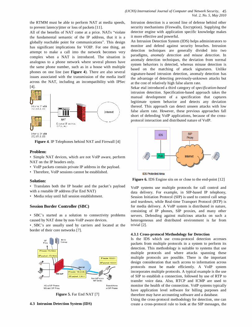
(IJCNS) International Journal of Computer and Network Security, Vol. 2, No. 5, May 2010
45
the RTMM must be able to perform NAT at media speeds, to prevent latency/jitter or loss of packets [11]. All of the benefits of NAT come at a price. NATs “violate the fundamental semantic of the IP address, that it is a globally reachable point for communications”. This design has significant implications for VOIP. For one thing, an attempt to make a call into the network becomes very complex when a NAT is introduced. The situation is analogous to a phone network where several phones have the same phone number, such as in a house with multiple phones on one line (see Figure 4). There are also several issues associated with the transmission of the media itself across the NAT, including an incompatibility with IPSec [4].
Figure 4. IP Telephones behind NAT and Firewall [4]
Problem: • Simple NAT devices, which are not VoIP aware, perform NAT on the IP headers only. • VoIP packets contain private IP address in the payload. • Therefore, VoIP sessions cannot be established.
Solution: • Translates both the IP header and the packet’s payload with a routable IP address (Far End NAT) • Media relay until full session establishment. Session Border Controller (SBC) • SBC’s started as a solution to connectivity problems caused by NAT done by non-VoIP aware devices. • SBC’s are usually used by carriers and located at the border of their core networks [7].
Figure 5. Far End NAT [7]
4.3 Intrusion Detection System (IDS)
Intrusion detection is a second line of defense behind other security mechanisms (Firewalls, Encryption). Supplying the detector engine with application specific knowledge makes it more effective and powerful. An Intrusion Detection System (IDS) helps administrators to monitor and defend against security breaches. Intrusion detection techniques are generally divided into two paradigms, anomaly detection and misuse detection. In anomaly detection techniques, the deviation from normal system behaviors is detected, whereas misuse detection is based on the matching of attack signatures. Unlike signature-based intrusion detection, anomaly detection has the advantage of detecting previously-unknown attacks but at the cost of relatively high false alarm rate. Sekar etal introduced a third category of specification-based intrusion detection. Specification-based approach takes the manual development of a specification that captures legitimate system behavior and detects any deviation thereof. This approach can detect unseen attacks with low false alarm rate. However, these previous approaches fall short of defending VoIP applications, because of the cross-protocol interaction and distributed nature of VoIP.
Figure 6. IDS Engine sits on or close to the end-point [12] VoIP systems use multiple protocols for call control and data delivery. For example, in SIP-based IP telephony, Session Initiation Protocol (SIP) is used to control call setup and teardown, while Real-time Transport Protocol (RTP) is for media delivery. A VoIP system is distributed in nature, consisting of IP phones, SIP proxies, and many other servers. Defending against malicious attacks on such a heterogeneous and distributed environment is far from trivial [2]. 4.3.1 Cross-protocol Methodology for Detection Is the IDS which use cross-protocol detection accesses packets from multiple protocols in a system to perform its detection. This methodology is suitable to systems that use multiple protocols and where attacks spanning these multiple protocols are possible. There is the important design consideration that such access to information across protocols must be made efficiently. A VoIP system incorporates multiple protocols. A typical example is the use of SIP to establish a connection, followed by use of RTP to transfer voice data. Also, RTCP and ICMP are used to monitor the health of the connection. VoIP systems typically have application level software for billing purposes and therefore may have accounting software and a database. Using the cross-protocol methodology for detection, one can create a cross-protocol rule to look at the SIP messages, the

(IJCNS) International Journal of Computer and Network Security, Vol. 2, No. 5, May 2010
46
transaction messages between the accounting software and the database, and the RTP flows later on. Specifically, each of the following three conditions must hold [12]. 1. The SIP message should follow the correct format. 2. When the accounting software sends out a transaction to denote a call from user A to user B, check if user A has sent a SIP Call Initialization message to user B. If user A has not set up the call with a legitimate SIP Call Initialization message, then this condition will be violated. 3. Check the source/destination IP addresses of the subsequent RTP flows. Together with information from DNS and SIP Location Servers, we can reconfirm that each RTP flow has a corresponding legitimate call setup. 4.3.2 Stateful Methodology for Detection A second abstraction useful for VoIP systems in particular is stateful detection. Stateful detection implies building up relevant state within a session and across sessions and using the state in matching for possible attacks. It is important that the state aggregation be done efficiently so that the technique is applicable in high throughput systems, such as VoIP systems. A VoIP system maintains considerable amount of system state. The client side maintains state about all the active connections – when the connection was initiated, when it can be torn down, and what the properties of the connection are. The server side also maintains state relevant to billing, such as the duration of the call.
5. Encryption and IPsec The only focus on security of the network, protecting endpoints, other components, from malicious attacks is not enough for VoIP systems. Firewalls, IDS, NAT, and other such devices can help keep intruders from compromising a network, but firewalls are no defense against an internal hacker in [4]. Another layer of defense is necessary at the protocol level to protect the data itself. In VOIP, as in data networks, this can be accomplished by encrypting the packets at the IP level using IPsec. This way if anyone on the network, authorized or not, intercepts VOIP traffic not intended for them, these packets will be impossible to understand. The IPsec suite of security protocols and encryption algorithms is the standard method for securing packets against unauthorized viewers over data networks and will be supported by the protocol stack in IPv6. Hence, it is both logical and practical to extend IPsec to VOIP, encrypting the signal and voice packets on one end and decrypting them only when needed by their intended recipient. Also, several factors, including the expansion of packet size, ciphering latency, and a lack of QoS urgency in the cryptographic engine itself can cause an excessive amount of latency in the VOIP packet delivery. This leads to degraded voice quality, so once again there is a tradeoff between security and voice quality, and a need for speed. Fortunately, the difficulties are not insurmountable. IPsec can be incorporated into a SIP network with roughly a three-second additional delay in call setup times, an acceptable delay for many applications. This section explains the issues involved
in successfully incorporating IPsec encryption into VOIP services. 5.1 IPSec IPsec is the preferred form of VPN tunneling across the Internet. There are two basic protocols defined in IPsec: Encapsulating Security Payload (ESP) and Authentication Header (AH) (see Figure 7). Both schemes provide connectionless integrity, source authentication, and an anti-replay service. The tradeoff between ESP and AH is the increased latency in the encryption and decryption of data in ESP and a “narrower” authentication in ESP, which normally does not protect the IP header “outside” the ESP header, although Internet Key Exchange (IKE: Responsible for key agreement using public key cryptography) can be used to negotiate the security association (SA), which includes the secret symmetric keys. In this case, the addresses in the header (transport mode) or new/outer header (tunnel mode) are indirectly protected, since only the entity that negotiated the SA can encrypt/decrypt or authenticate the packets. Both schemes insert an IPsec header (and optionally other data) into the packet for purposes, such as authentication [4]. IPsec also supports two modes of delivery: Transport and Tunnel. Transport mode encrypts the payload (data) and upper layer headers in the IP packet. The IP header and the new IPsec header are left in plain sight. So if an attacker were to intercept an IPsec packet in transport mode, they could not determine what it contained; but they could tell where it was headed, allowing rudimentary traffic analysis. On a network entirely devoted to VOIP, this would equate to logging which parties were calling each other, when, and for how long. Tunnel mode encrypts the entire IP datagram and places it in a new IP Packet [9]. Both the payload and the IP header are encrypted. The IPsec header and the new IP Header for this encapsulating packet are the only information left in the clear.
Figure 7. IPsec Tunnel and Transport Modes [9] IPSec supports the Triple DES encryption algorithm (168-bit) in addition to 56-bit encryption. Triple DES (3DES) is a strong form of encryption that allows sensitive information to be transmitted over untrusted networks. It enables

(IJCNS) International Journal of Computer and Network Security, Vol. 2, No. 5, May 2010
47
customers, particularly in the finance industry, to utilize network layer encryption.
Table 1: Encryption Algorithms for VoIP [9]
5.2 The Role of IPSec in VOIP The prevalence and ease of packet sniffing and other techniques for capturing packets on an IP based network makes encryption a necessity for VOIP. Security in VOIP is concerned both with protecting what a person says as well as to whom the person is speaking. IPSec can be used to achieve both of these goals as long as it is applied with ESP using the tunnel method. This secures the identities of both the endpoints and protects the voice data from prohibited users once packets leave the corporate intranet. The incorporation of IPSec into Ipv6 will increase the availability of encryption, although there are other ways to secure this data at the application level. VOIPsec (VOIP using IPSec) helps reduce the threat of man in the middle attacks, packet sniffers, and many types of voice traffic analysis. Combined with the firewall implementations, Ipsec makes VOIP more secure than a standard phone line. It is important to note, however, that Ipsec is not always a good fit for some applications, so some protocols will continue to rely on their own security features. 5.3 Local VPN Tunnels Virtual Private Networks (VPNs) are “tunnels” between two endpoints that allow for data to be securely transmitted between the nodes. The IPSec ESP tunnel is a specific kind of VPN used to traverse a public domain (the Internet) in a private manner. The use and benefits of VPNs in IPSec have been great enough for some to claim “VOIP is the killer app for VPNs”. VPN tunnels within a corporate LAN or WAN are much more secure and generally faster than the IPSec VPNs across the Internet because data never traverses the public domain, but they are not scaleable [4]. Also, no matter how the VPN is set up, the same types of attacks and issues associated with IPSec VPNs are applicable, so we consider here only the case of IPSec tunneling and assume the security solutions can be scaled down to an internal network if needed. 5.4 Memory and CPU Considerations Packets that are processed by IPSec are slower than packets that are processed through classic crypto. There are several reasons for this and they might cause significant performance problems: 1. IPSec introduces packet expansion, which is more likely
to require fragmentation and the corresponding reassembly of IPSec datagrams. 2. Encrypted packets are probably authenticated, which means that there are two cryptographic operations that are performed for every packet. 3. The authentication algorithms are slow, although work has been done to speed up things as the Diffie−Hellman computations [4]. 5.5 Difficulties Arising from VOIPsec IPSec has been included in IPv6. It is a reliable, robust, and widely implemented method of protecting data and authenticating the sender. However, there are several issues associated with VOIP that are not applicable to normal data traffic. Of particular interest are the Quality of Service (QoS) issues and some others like latency, jitter, and packet loss. These issues are introduced into the VOIP environment because it is a real time media transfer, with only 150 ms to deliver each packet. In standard data transfer over TCP, if a packet is lost, it can be resent by request. In VOIP, there is no time to do this. Packets must arrive at their destination and they must arrive fast. Of course the packets must also be secure during their travels. However, the price of this security is a decisive drop in QoS caused by a number of factors. A study by researchers focused on the effect of VOIPsec on various QoS issues and on the use of header compression as a solution to these problems. They studied several codecs, encryption algorithms, and traffic patterns to garner a broad description of these effects. Some empirical results developed by Cisco are available as well in [4]. Delay • Processing—PCM to G.729 to packet • Encryption — ESP encapsulation + 3DES • Serialization — time it takes to get a packet out of the router, each “hop” generally has fixed delay. • IPsec overhead: about 40 bytes (depending configuration) • IP header: 20 bytes • UDP + RTP headers: 20 bytes • RTP header compression: 3 bytes for IP+UDP+RTP Effects on 8 kbps CODEC (voice data: 20 bytes) • clear text voice has an overhead of 3 bytes, which suggests required bandwidth of approximately 9 kbps • IPsec encrypted voice: overhead 80 bytes and required bandwidth 40 kbps 5.6 Encryption / Decryption Latency The cryptographic engine is bottleneck for voice traffic transmitted over IPsec. The driving factor in the degraded performance produced by the cryptography was the scheduling algorithms in the crypto-engine itself However, there still was significant latency due to the actual encryption and decryption. Encryption/decryption latency is a problem for any cryptographic protocol, because much of it results from the computation time required by the underlying encryption. With VOIP’s use of small packets at a fast rate and
Encryption Algorithms for IPSec Type Key Strengt
h DES Symmetric 56-bit Weak
3DES Symmetric 168-bit Medium
AES Symmetric 128, 192, or 256-bit
Strong
RSA Asymmetric 1024-bit minimum Strong

(IJCNS) International Journal of Computer and Network Security, Vol. 2, No. 5, May 2010
48
intolerance for packet loss, maximizing throughput is critical. However, this comes with a price, because although DES is the fastest of these encryption algorithms, it is also the easiest to crack [4]. Thus, designers are once again forced to toe the line between security and voice quality.
5.7 Expanded Packet Size IPsec also increases the size of packets in VOIP, which leads to more QoS issues. The increase is actually just an increase in the header size due to the encryption and encapsulation of the old IP header and the introduction of the new IP header and encryption information. This leads to several complications when IPsec is applied to VOIP. First, the effective bandwidth is decreased as much as 63% [4]. Thus connections to single users in low bandwidth areas (i.e. via modem) may become infeasible. The size discrepancy can also cause latency and jitter issues as packets are delayed by decreased network throughput or bottlenecked at hub nodes on the network (such as routers or firewalls).
5.8 IPsec and NAT Incompatibility IPsec and NAT compatibility is far from ideal. NAT traversal completely invalidates the purpose of AH because the source address of the machine behind the NAT is masked from the outside world. Thus, there is no way to authenticate the true sender of the data. The same reasoning demonstrates the inoperability of source authentication in ESP. We have defined this as an essential feature of VOIPsec, so this is a serious problem. There are several other issues that arise when ESP traffic attempts to cross a NAT. If only one of the endpoints is behind a NAT, the situation is easier. If both are behind NATs, IKE negotiation can be used for NAT traversal, with UDP encapsulation of the IPsec packets.
6. Solutions to the VOIPsec Issues We have raised a number of significant concerns with IPsec’s role in VOIP. However, many of these technical problems are solvable. Despite the difficulty associated with these solutions it is very important for the establishment of a secure implementation of VOIPsec.
6.1 Encryption at the End Points One proposed solution to the bottlenecking at the routers due to the encryption issues is to handle encryption/decryption solely at the endpoints in the VOIP network. One consideration with this method is that the endpoints must be computationally powerful enough to handle the encryption mechanism. Though ideally encryption should be maintained at every hop in a VOIP packet’s lifetime, this may not be feasible with simple IP phones with little in the way of software or computational power. In such cases, it may be preferable for the data be encrypted between the endpoint and the router (or vice versa) but unencrypted traffic on the LAN is slightly less damaging than unencrypted traffic across the Internet [4]. Fortunately, the increased processing power of newer
phones is making endpoint encryption less of an issue.
6.2 Secure Real Time Protocol (SRTP) The Secure Real-time Protocol is a profile of the Real-time Transport Protocol (RTP) offering not only confidentiality, but also message authentication, and replay protection for the RTP traffic as well as RTCP (Real-time Transport Control Protocol). SRTP provides a framework for encryption and message authentication of RTP and RTCP streams. SRTP can achieve high throughput and low packet expansion. SRTP is independent of a specific RTP stack implementation and of a specific key management standard, but Multimedia Internet Keying (MIKEY) has been designed to work with SRTP. In comparison to the security options for RTP there are some advantages to using SRTP. The advantages over the RTP standard security and also over the H.235 security for media stream data are listed below [4, 12]. SRTP provides increased security, achieved by • Confidentiality for RTP as well as for RTCP by encryption of the respective payloads; • Integrity for the entire RTP and RTCP packets, together with replay protection; • The possibility to refresh the session keys periodically, which limits the amount of cipher text produced by a fixed key, available for an adversary to cryptanalyze; • An extensible framework that permits upgrading with new cryptographic algorithms; • A secure session key derivation with a pseudo-random function at both ends; • The usage of salting keys to protect against pre-computation attacks; • Security for unicast and multicast RTP applications. SRTP has improved performance attained by • Low computational cost asserted by pre-defined algorithms; • Low bandwidth cost and a high throughput by limited packet expansion and by a framework preserving RTP header compression efficiency; • Small footprint that is a small code size and data memory for keying information and replay lists. 6.3 Key Management for SRTP – MIKEY SRTP uses a set of negotiated parameters from which session keys for encryption, authentication and integrity protection are derived. MIKEY describes a key management scheme that addresses real-time multimedia scenarios (e.g. SIP calls and RTSP sessions, streaming, unicast, groups, multicast). The focus lies on the setup of a security association for secure multimedia sessions including key management and update, security policy data, etc., such that requirements in a heterogeneous environment are fulfilled. MIKEY also supports the negotiation of single and multiple crypto sessions.

(IJCNS) International Journal of Computer and Network Security, Vol. 2, No. 5, May 2010
49
MIKEY has some important properties in [4]: • MIKEY can be implemented as an independent software library to be easily integrated in a multimedia communication protocol. It offers independency of a specific communication protocol (SIP, H.323, etc.) • Establishment of key material within a 2-way handshake, therefore best suited for real-time multimedia scenarios There are four options for Key Distribution: • Pre-shared key • Public-key encryption • Diffie-Hellman key exchange protected by public-key encryption • Diffie-Hellman key exchange protected with pre-shared-key and keyed hash functions (using an MIKEY extension (DHHMAC))
6.4 Better Scheduling Schemes Without a way for the crypto-engine to prioritize packets, the engine will still be susceptible to DoS attacks and starvation from data traffic impeding the time-urgent VOIP traffic. A few large packets can clog the queue long enough to make the VOIP packets over 150 ms late (sometimes called head-of-line blocking), effectively destroying the call. Ideally, the crypto-engine would implement QoS scheduling to favor the voice packets, but this is not a realistic scenario due to speed and compactness constraints on the crypto-engine. One solution implemented in the latest routers is to schedule the packets with QoS in mind prior to the encryption phase. It is not surprising that for voice traffic the crypto-engine can be a serious bottleneck. Rather than the expected constraints on the crypto-engine throughput, the critical factor turned out to be the impossibility to control and schedule access to the crypto-engine so as to favor real-time traffic over regular one. This applies regardless of whether the scheduler is implemented as a software module or a hardware component. Therefore, if voice traffic is interleaved with other types of traffic, e.g., ftp or http traffic, during a secure session, it may happen that the latter (usually characterized by big packets) is scheduled in the crypto-engine before voice traffic. In this case voice traffic might be delayed to the point that packets are discarded most of the times.
6.5 Compression of Packet Size Compression of Packet Size turn results in considerably less jitter, latency, and better crypto-engine performance. There is, of course, a price for these speedups. The compression scheme puts more strain on the CPU and memory capabilities of the endpoints in order to achieve the compression, and, of course, both ends of a connection must use the same compression algorithm. Efficient solution for packet header compression is known as cIPsec, for VoIPsec traffic. Simulation results from different sources show that the proposed compression scheme significantly reduces the overhead of packet headers, thus increasing the effective bandwidth used by the
transmission. In particular, when cIPsec is adopted, the average packet size is only 2% bigger, rather than 50% longer plain VoIPsec packets, which makes VoIPsec and VoIP equivalent from the bandwidth usage point of view. However, packet loss does have an exacerbated detrimental effect on packets compressed under the cIPsec scheme. When packets are lost, they cannot be re-sent and the endpoints need to resynchronize. However, the time saved in the crypto-engine and the security provided may be well worth this price of this approach [5].
6.6 Resolving NAT/IPSec Incompatibilities The most likely widespread solution to the problem of NAT traversal is UDP encapsulation of IPSec. This implementation is supported by the IETF and effectively allows all ESP traffic to traverse the NAT. In tunnel mode, this model wraps the encrypted IPSec packet in a UDP packet with a new IP header and a new UDP header, usually using port 500. This port was chosen because it is currently used by IKE peers to communicate so overloading the port does not require any new holes to be punched in the firewall. The SPI field within the UDP-encapsulated packet is set to zero to differentiate it from an actual IKE communication. This solution allows IPsec packets to traverse standard NATs in both directions. The adoption of this standard method should allow VOIPsec traffic to traverse NATs cleanly, although some extra overhead is added in the encapsulation/decapsulation process. IKE negotiation will also be required to allow for NAT traversal. The problem still remains that IP-based authentication of the packets cannot be assured across the NAT, (although fully qualified domain names could be used) but the use of a shared secret (symmetric key) negotiated through IKE could provide authentication. It is important to note that IP-based authentication is weak compared with methods using cryptographic protocols. There are several other solutions to the IPsec/NAT incompatibility problem, including Realm-Specific IP RSIP), IPv6 Tunnel Broker, IP Next Layer (IPNL), and UDP encapsulation. RSIP is designed as a replacement for NAT and provides a clear tunnel between hosts and the RSIP Gateway. RSIP supports both AH and ESP, but implementing RSIP would require a significant overhaul of the current LAN architecture so while it is quite an elegant solution, it is currently infeasible. Perhaps as a result of these problems, RSIP is not widely used. The IPv6 tunnel broker method uses an IPv6 tunnel as an IPSec tunnel, and encapsulates an IPv6 packet in an IPv4 packet. But this solution also requires LAN upgrades and doesn’t work in situations where multiple NATs are used. IPNL introduces a new layer into the network protocols between IP and TCP/UDP to solve the problem, but IPNL is in competition with IPv6 and IPv6 is a much more widely used standard [4].

(IJCNS) International Journal of Computer and Network Security, Vol. 2, No. 5, May 2010
50
7. Security Threats in VoIP In the early days of VoIP, there was no big concern about security issues related to its use. People were mostly concerned with its cost, functionality and reliability. Now that VoIP is gaining wide acceptance and becoming one of the mainstream communication technologies, security has become a major issue. The security threats cause even more concern when we think that VoIP is in fact replacing the oldest and most secure communication system the world ever known – POTS (Plain Old Telephone System). Let us have a look at the threats VoIP users face.
7.1 Identity and Service Theft Service theft can be exemplified by phreaking, which is a type of hacking that steals service from a service provider, or use service while passing the cost to another person. Encryption is not very common in SIP, which controls authentication over VoIP calls, so user credentials are vulnerable to theft. Eavesdropping is how most hackers steal credentials and other information. Through eavesdropping, a third party can obtain names, password and phone numbers, allowing them to gain control over voicemail, calling plan, call forwarding and billing information. This subsequently leads to service theft. Stealing credentials to make calls without paying is not the only reason behind identity theft. Many people do it to get important information like business data. A phreaker can change calling plans and packages and add more credit or make calls using the victim’s account. He can of course as well access confidential elements like voice mail, do personal things like change a call forwarding number [10].
7.2 Vishing Vishing is another word for VoIP Phishing, which involves a party calling you faking a trustworthy organization (e.g. your bank) and requesting confidential and often critical information.
7.3 Viruses and Malware VoIP utilization involving soft-phones and software are vulnerable to worms, viruses and malware, just like any Internet application. Since these soft-phone applications run on user systems like PCs and PDAs, they are exposed and vulnerable to malicious code attacks in voice applications.
7.4 DoS (Denial of Service) A DoS attack is an attack on a network or device denying it of a service or connectivity. It can be done by consuming its bandwidth or overloading the network or the device’s internal resources. In VoIP, DoS attacks can be carried out by flooding a target with unnecessary SIP call-signaling messages, thereby
degrading the service. This causes calls to drop prematurely and halts call processing. Why would someone launch a DoS attack? Once the target is denied of the service and ceases operating, the attacker can get remote control of the administrative facilities of the system [10, 12].
7.5 Spamming over Internet Telephony (SPIT) If you use email regularly, then you must know what spamming is. Put simply, spamming is actually sending emails to people against their will. These emails consist mainly of online sales calls. Spamming in VoIP is not very common yet, but is starting to be, especially with the emergence of VoIP as an industrial tool. Every VoIP account has an associated IP address. It is easy for spammers to send their messages (voicemails) to thousands of IP addresses. Voice mailing as a result will suffer. With spamming, voicemails will be clogged and more space as well as better voicemail management tools will be required. Moreover, spam messages can carry viruses and spyware along with them. [10]
7.6 Call Tampering Call tampering is an attack which involves tampering a phone call in progress. For example, the attacker can simply spoil the quality of the call by injecting noise packets in the communication stream. He can also withhold the delivery of packets so that the communication becomes spotty and the participants encounter long periods of silence during the call.
7.7 Man-in-the-Middle Attacks VoIP is particularly vulnerable to man-in-the-middle attacks, in which the attacker intercepts call-signaling SIP message traffic and masquerades as the calling party to the called party, or vice versa. Once the attacker has gained this position, he can hijack calls via a redirection server [10]. 8. Conclusion This paper provides an overview of the VoIP and of the issues related to VoIP security. There are numerous challenges to the secure implementation, deployment and use of the VoIP on a same network which is used to carry other network data. These challenges are related to the service availability, Quality of Service, Firewalls, Intrusion Detection, IPSec, VoIP threats, and privacy. The next step for the ongoing research project is to identify specific areas that will be addressed in the near term research efforts. References [1] Rinzam A. VoIP: Voice Over Internet Protocol.
Department of Computer Science and Engineering, M G College of Engineering.
[2] H. Sengar, D. Wijesekera. Center for Secure Information Systems, George Mason University, Fairfax, USA. H. Wang, S. Jajodia. Department of CS, College of William and Mary, Williamsburg, USA. “IDS: VoIP
(IJCNS) International Journal of Computer and Network Security, Vol. 2, No. 5, May 2010
51
Intrusion Detection through Interacting Protocol State Machines”.
[3] M. Marjalaakso. Security Requirements and Constraints of VoIP. Helsinki University of Technology, Department of Electrical Engineering and Telecommunications.
[4] D. Richard Kuhn, Thomas J. Walsh, and Steffen Fries, “Security Considerations for Voice Over IP Systems: Recommendations of the National Institute of Standards and Technology” Special Publication 800-58, Sections 8 and 9, January 2005.
[5] R. Barbieri, D. Bruschi, E. Rosti. Voice over IPsec: Analysis and Solutions. Department of Science, University of Milano, Itlay.
[6] G. Egeland, “Introduction to IPsec in IPv6”. http://www.eurescom.de/~publicwebdeliverables/P1100series/P1113/D1/pdfs/pir1/41_IPsec_intro.pdf
[7] Check Point Software Technologies Ltd. “Check Point Solution for Secure VoIP”. 2003 - 2007.
[8] NAT: Network Address Translation and Voice Over Internet Protocol. http://www.voip-info.org/wiki/view/NAT+and+VOIP
[9] Jeremy Stretch. IPSEC: Internet Protocol Security. http://www. packetlife.net
[10] M. Hurley. “VoIP VULNERABILITIES”. Centre for Critical Infrastructure Protection (CCIP). Information Note, Issue 06, Wellington, New Zealand, January 2007.
[11] Mark D. Collier. Firewall Requirements for Securing VoIP, SecureLogix Corporation.www.securelogix.com
[12] Yu-Sung Wu, S. Bagchi. School of Electrical & Computer Eng, Purdue University, S. Garg, N. Singh, Tim Tsai, Avaya Labs. “A Stateful and Cross Protocol Intrusion Detection Architecture for VoIP Environments”.
Authors Profile
Ali Tahir is an MS Scholar at University of Engineering and Technology, Taxila, Pakistan. He did his B.Sc Software Engineering from UET TAXILA in 2005. He has worked in Nokia Siemens Network for two years as an implementation engineer. Currently he is working in cryptography and network security center at a Government organization. His areas
of interest are digital image processing, computer vision, network security and wireless communication.
Asim Shahzad is pursuing his PhD from University of Engineering and Technology Taxila, Pakistan. He has also completed his MS in Computer Engineering from UET TAXILA. He has done MS in Telecommunication Engineering from institute of communication technologies, Islamabad, Pakistan. He is working as
Assistant Professor at UET TAXILA in Telecommunication Engineering Department. His areas of interest are optical communication, Data and network Security.

(IJCNS) International Journal of Computer and Network Security, Vol. 2, No. 5, May 2010
52
A Novel Run-Time Memory Leak Detection and Recovery (MLDR) Using Aging in Physical
Memory Space
Ahmed Otoom1, Mohammad Malkawi2 and Mohammad Alweh3
1Royal Jordanian Air Force, IT Directorate, Amman 11134, Jordan
2Middle East University Amman, Jordan
3 Southern Illinois State University Carbondale, Illinois, USA
[email protected] Abstract: This paper provides a novel run-time approach for memory leak detection and recovery (MLDR) using aging in physical memory space. MLDR algorithm reflects both the physical and virtual behavior of memory allocation and benefits from the hardware support available for tracking physical pages in real memory in order to detect leak in virtual address space.
MLDR detects stale and unreachable memory objects. A conservative implementation of MLDR recovers only unreachable leaky objects in order to avoid the potential false positives stale objects. MLDR has a coarse granularity in the sense that it deals with pages rather than memory chunks, thus enabling it to avoid costly scans of heap allocation. Simulation results show the effectiveness of MLDR in detecting and recovering memory leaks at run time.
Keywords: memory leak detection, memory leak recovery,
memory aging, and dynamic memory management.
1. Introduction Several approaches for solving memory leak have been developed including static analysis tools, dynamic tools, and automatic dynamic tools. Static analysis tools [1], [7] are used to identify leaks in development environment before executing the program; they do not cause any run time overhead. These tools lack dynamic information so they produce false positives and can not find all leaks. Some dynamic tools [10] analyze memory consumption interactively by inspecting and comparing snapshots of the heap. They allow for the search for causes of leaked objects at runtime environments and facilitate the use of garbage collection. Automatic dynamic tools report the leaked objects and leak sites at the end of the program run. Some tools [4] instrument allocation functions to report immortal objects. Insure++ [8] uses a reference counting garbage collection approach to detect where the last reference to an object disappears. Others [11] instrument allocation function and use mark and sweep garbage collectors to capture unreachable objects. These tools either miss many leaks or incur high overhead cost. Besides operating outside the run time environment, the current approaches have relatively high overhead cost. The concept of detecting leak based on
object access is used in SWAT [15]. SWAT is an automatic dynamic memory leak detection tool that traces memory allocations/frees to build a heap model and uses an adaptive statistical profiling approach to monitor loads/stores to these objects. Objects that are not accessed for a long time are reported as leaks. This tool detects leaks with a less than 10% false positive rate. Leaks are reported at the end of an application run; SWAT can not decide on its own to deallocate them.
Different businesses can deal with software failures in different ways. In some cases, system administrators simply restart the system whenever the memory leaks to a point where a crash is imminent or performance degrades beyond an acceptable level. Systems with critical applications can not tolerate the cost of frequent shutdowns or performance degradation. For example, rebooting and restarting the software systems such as the Patriot Software [3] every 8 hours was responsible for losing lives during the first Gulf War. The consequences of unresolved memory leaks in real-time systems can have a direct impact on human safety, security and business sustainability.
This paper introduces a new memory leak detection and recovery (MLDR) algorithm. MLDR provides a run-time solution; it helps recover leaky objects which results in enhancing the system performance and making mission critical programs live longer. The main concept underlying the design of MLDR is the concept of memory objects aging in the physical space rather than in the virtual space.
Software aging, in general, refers to source contention issues that can cause performance degradation or can cause systems to hang, panic, or crash. Software aging mechanisms can include memory leaks, unreleased file locks, accumulation of unterminated threads, data corruption/round-off accrual, file space fragmentation, shared memory pool latching, and others [6], [13], [14]. Parnas [9] documents software aging as a phenomenon wherein legacy software becomes difficult to maintain as it ages.
Aging, in this paper, refers to the time a piece of memory object remains untouched. A leaky object by definition will
(IJCNS) International Journal of Computer and Network Security, Vol. 2, No. 5, May 2010
53
begin to age since it will no longer be accessed by any application program. Aging, in this context, can then be used to detect memory leakage. Memory leaks and aging refer to objects in the heap virtual space. Detecting leaky objects by estimating their age in the virtual space [15] is time consuming. However, detecting the age of a page in the physical space is much less time consuming and can be done using the already available support for virtual memory systems. MLDR makes use of page aging in the physical space to detect actual leaks in the virtual space. Hence, MLDR can be used to detect and recover leaks at run time reducing the risk of performance degradation or crashes.
This paper is organized as follows. Section 2 presents the new memory leak detection and recovery algorithm (MLDR). Section 3 presents a simulation model to measure the performance and effectiveness of MLDR. Section 4 presents a summary of the conclusions.
2. Memory Leak Detection and Recovery (MLDR) Using Aging in Physical Memory
2.1 Background A memory object is said to have leaked if it is not freed by the program or the system after it becomes no longer used or accessible. The main job for a memory leak detector is to determine whether an object has leaked at a given point of time. In most general terms, memory leak occurs because of 1) unreachable objects: a program either unintentionally or maliciously neglects to free heap-allocated objects and therefore these objects are lost. In this case, there is no reference chain for these objects from the root set starting from global and stack variables and 2) useless objects: a program maintains references to objects which are never used again.
The memory leak detection and recovery (MLDR) algorithm is able to detect both types (unreachable and useless/stale objects). In this paper, we present two versions of MLDR; a conservative one which recovers only unreachable objects, and a liberal version which recovers both unreachable and stale objects. The conservative approach does not produce false positives, i.e, falsely identified leaks. The liberal approach produces false positives, mostly related to stale objects. Recovering stale objects without incurring false positives is more complicated and requires significant architectural changes, and will not be discussed in this paper.
MLDR has a coarse granularity in the sense that it deals with pages instead of memory chunks. Hence, we introduce the term “leaky page” where a leaky page is a page which contains potentially leaky chunks. A leaky page may contain any combination of the following types of objects: 1) unreachable objects and 2) stale objects. In the context of this paper, stale objects are objects that have not been accessed for a given period of time. They are either a) useless objects or b) active but have not been referenced for that period of time. In our approach, the MLDR leak detection mechanism identifies the potential leaky pages. Depending on the page size and the sizes of allocated memory chunks, a page may contain several memory
chunks or the page may constitute a portion of one memory chunk.
The recovery mechanism of the conservative MLDR identifies unreachable objects from the set of leaky pages. The remaining objects are stale objects. The unreachable objects are relinquished (freed) and returned to the operating system.
MLDR is particularly useful in long lived applications. As time passes, age accumulates and MLDR will be able to identify a set of unreachable objects. These objects will be freed which makes enough room for new allocations and enables the program to continue execution. Another consequence of memory leak is thrashing. Memory leak can cause extreme low locality of reference as live objects are dispersed over a large virtual address space. MLDR will relinquish unreachable locations causing the operating system to reuse these locations and enhance the locality of reference as a result.
2.2 Description of MLDR Once a memory object has leaked, it will no longer be accessed by the application program. Hence, a leaky memory object will begin to age. Aging, in this context, is related to the time a piece of memory remains untouched. In virtual memory computer systems, memory allocation is done both at the virtual and physical levels. A memory leakage in the virtual space will render the corresponding mapped physical memory in a “page-out status”. A page-out status makes a page in the physical memory a target for the replacement policy that swaps the target page out to disk. Going backward, a swapped out page can correspond, but not necessarily, to a leaked chunk in the virtual space. We define “the age of a page” as the time elapsed since the page is swapped out from the physical to the virtual space. More precisely, the age of a page begins to accumulate from the time a page is marked by the replacement policy as a target for replacement. Note that a page may remain in the physical space for a long time after it has been marked as a replaceable page. A memory chunk will be considered a candidate leak if the age of the page to which it belongs exceeds a certain limit (threshold). This threshold can be either user-defined or tuned by a telemetry tool.
Memory leak detection policies can rely on memory aging either in the virtual or physical space. Aging in the virtual space is more accurate than aging in the physical space; however, using the concept of physical space aging has several advantages. The physical space is much smaller than the virtual address space, which makes the time required to scan for leaky pages much less than the time needed to search for leaky chunks in the virtual space. Also, tracing the age of a page in the physical space can greatly benefit from the available hardware support for virtual memory organization such as page tables and address translation buffers. Of course, the age of a page in the physical space may not be entirely due to the behavior of the owner of the page; it might well depend on the behavior of other programs as well as on the page replacement policy (LRU, FIFO, OPT, LFU) [12] deployed by the operating system.
It should be noted that several chunks, whose sizes are smaller than a page, may be mapped to one physical page. If
(IJCNS) International Journal of Computer and Network Security, Vol. 2, No. 5, May 2010
54
only one of these chunks remains active, while the other chunks have leaked, then the corresponding page will be considered active and the leaks in that page will not be detected; this case is known as “false negative”. We show in this paper how the problem of false negatives can be reduced.
2.3 MLDR Algorithm Main Functions MLDR algorithm utilizes the following functions: Main(), Initialize(), Bookkeeping(), StalenessDetector(), StalenessRecovery(), and new versions of malloc() and free() functions.
2.3.1 Main() and Initialize() Functions The “main()” function of the algorithm keeps iterating over monitored processes. Main() calls two functions: Initialize() and Bookkeeping(). For each monitored process, the Initialize() function sets some user-configurable parameters that affect the behavior of the MLDR algorithm. These parameters can be user-configurable or they can be automatically tuned using a telemetry tool. These parameters are: upper heap size threshold(UHST), lower heap size threshold(LHST), staleness detector sleeps time(SDST), and a normalized parameter(K). The UHST is used to initiate the leak detection process once the size of the heap for the monitored process exceeds the UHST limit. The LHST is used to suspend the detection and recovery process once the current heap size drops below LHST. The SDST is the time (in milliseconds) a StalenessDetector() will wait between any two successive scans to the page table of a given process. The page age threshold(PAT) is used to identify aged pages. When the age of a page exceeds PAT, it will be marked as a candidate leaky page. PAT is calculated dynamically as an accumulated average and is fine-tuned using the K parameter.
2.3.2 Bookkeeping() Function The page table is augmented with a new entry called timestamp(TS). For every victim page selected from the mapped physical space, the bookkeeping() function timestamps the corresponding page in the virtual address space by setting the TS to the current time. The TS is used to calculate the age of a page. Whenever a page is paged back into physical memory, the TS entry is reset to zero. Pages whose TS value is larger than zero begin to age as time progresses.
2.3.3 Memory Allocation and Deallocation Functions For implementation purposes, we need to modify memory allocation and deallocation functions, e.g., malloc() and free(). Other functions are treated in a similar manner, and hence will not be provided in this paper.
(a) malloc () Function The malloc() function incorporates two major changes before it returns a pointer to the newly allocated memory chunk. The first, Malloc() checks the heap size and if the UHST is reached, it invokes the StalenessDetector(). The StalenessDetector() is suspended when the heap size reaches the lower limit LHST. This modification to malloc() helps reducing the overhead associated with leak detection and recovery.
The latter, the execution of malloc() updates the entries of a table called “MallocTable” which includes the address
of the allocated chunk, its size and a flag. The flag is initially set to one, indicating that the object is alive and reachable. The flag is reset to zero by the StalenessRecovery() function as a result of scanning the stack and registers. If a memory chunk in the MallocTable is not matched by any address value in the stack and address registers, then the corresponding flag is set to zero, and the chunk is deemed unreachable.
(b) free() Function Before deallocating a chunk of memory and exiting, the free() function removes the deallocated chunk from the MallocTable; these are objects with flag value reset to zero.
2.3.4 StalenessDetector() Function The StalenessDetector() traverses the page table of a given process in order to identify leaky pages. It identifies all pages whose age has exceeded the page age threshold (PAT). Note that any identified page at this phase is considered to be only a candidate leaky page, meaning that it may or may not contain leaky chunks. A memory chunk contained in a leaky page could in fact be active, but has not been referenced for a relatively long time, such that the aging algorithm marked their corresponding page as a leaky page; this is a case of “false positive”.
2.3.5 StalenessRecovery() Function. StalenessRecovery() works on the set of identified leaky pages(aged pages). Its main task is to remove unreachable objects, given that a leaky page is found to include a leak. In order to identify the set of chunks in a leaky page, the StalenessRecovery() intersects the MallocTable with the range of addresses in that page [page_number * PAGE_SIZE, (page_number+1)*PAGE_SIZE-1]. The result of intersection (working set), will contain the potential leaky chunks. Unreachable chunks in the working set will be identified by scanning the roots (static, stack, and registers) searching for reachable objects in the given set of leaky pages. Once reachable objects are identified, the remaining objects in this set are definitely unreachable. Identified unreachable chunks are passed to the free function to be deallocated from the virtual address space and from the MallocTable, respectively. The remaining chunks in the working set are stale objects. The conservative version of MLDR ignores all stale objects in order to avoid running the risk of false positives.
2.4 False Positives and False Negatives 2.4.1 False Positives
One of the main problems in memory leak detection tools is the potential error known as “false positives”. In other words, a detected leak is not a real leak. Since MLDR is a run-time solution it is not recommended to deallocate chunks which may turn out to be false positives. This is especially true for systems running critical applications. Referencing an object after it has been removed or deallocated leads to incorrect results or program crash. MLDR identifies potential leaky pages which might contain false positive objects. In order to avoid the consequences of false positives, the set of leaky pages are passed to the StalenessRecovery() which identifies and recovers unreachable objects. Of course, the leaky but reachable (stale) objects will persist in the system and will be counted as false negatives. The liberal approach would consider all
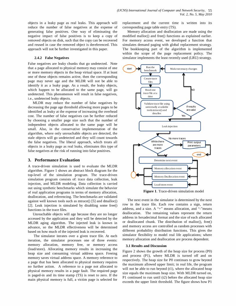
(IJCNS) International Journal of Computer and Network Security, Vol. 2, No. 5, May 2010
55
objects in a leaky page as real leaks. This approach will reduce the number of false negatives at the expense of generating false positives. One way of eliminating the negative impact of false positives is to keep a copy of removed objects on disk, such that the copy can be recovered and reused in case the removed object is dereferenced. This approach will not be further investigated in this paper.
2.4.2 False Negatives False negatives are leaky chunks that go undetected. Note that a page allocated to physical memory may consist of one or more memory objects in the heap virtual space. If at least one of these objects remains active, then the corresponding page may never age and the MLDR will not be able to identify it as a leaky page. As a result, the leaky objects, which happen to be allocated to the same page, will go undetected. This phenomenon will result in false negatives, i.e., undetected leaky objects.
MLDR may reduce the number of false negatives by decreasing the page age threshold allowing more pages to be identified as leaky at the expense of increasing the overhead cost. The number of false negatives can be further reduced by choosing a smaller page size such that the number of independent objects allocated to the same page will be small. Also, in the conservative implementation of the algorithm, where only unreachable objects are detected, the stale objects will go undetected and they will count towards the false negatives. The liberal approach, which treats all objects in a leaky page as real leaks, eliminates this type of false negatives at the risk of running into false positives.
3. Performance Evaluation A trace-driven simulation is used to evaluate the MLDR algorithm. Figure 1 shows an abstract block diagram for the top-level of the simulation program. The trace-driven simulation program consists of: trace data collection, leak injection, and MLDR modeling. Data collection is carried out using synthetic benchmarks which simulate the behavior of real application programs in terms of memory allocation, deallocation, and referencing. The benchmarks are validated against well known tools such as mtrace() [5] and dmalloc() [2]. Leak injection is simulated by disabling some free() functions in the trace files.
Unreachable objects will age because they are no longer accessed by the application and they will be detected by the MLDR aging algorithm. The injected leak is known in advance, so the MLDR effectiveness will be determined based on how much of the injected leak is recovered.
The simulator iterates over a given trace file. At each iteration, the simulator processes one of three events: memory allocation, memory free, or memory access (load/store). Allocating memory results in increasing the heap size and consuming virtual address space. Freeing memory saves virtual address space. A memory reference to a page that has been allocated to physical memory requires no further action. A reference to a page not allocated to physical memory results in a page fault. The required page is paged-in and its time stamp (TS) is reset to zero. If the main physical memory is full, a victim page is selected for
replacement and the current time is written into its corresponding page table entry (TS).
Memory allocation and deallocation are made using the modified malloc() and free() functions as explained earlier. For memory access event, we developed a function that simulates demand paging with global replacement strategy. The bookkeeping part of the algorithm is implemented within the scope of the page replacement policy. The simulator implements the least recently used (LRU) strategy.
start Run the benchmark
Create trace files
Read one trace file a t a
time
Validate trace file using universally available
tools mtrace() and dma lloc
if results are valid
Make necessa ry cha nges
NO
Leak injection
Yes
While there are more
traces
No more traces
end
Determine next event
Load/store event
Memory Dea llocation event
Memory alloca tion event
Print output parameters
Figure 1. Trace-driven simulation model
The next event in the simulator is determined by the next
row in the trace file. Each row contains a sign, return address, and a size. A “+” means allocation, and “-”means deallocation. The remaining values represent the return address in hexadecimal format and the size of each allocated or deallocated chunk. The distribution of malloc(), free() and memory access are controlled as random processes with different probability distribution functions. This gives the simulator flexibility to model real life applications; where memory allocation and deallocation are process dependent.
3.1 Results and Discussion Figure 2 shows the growth of the heap size for process (P0) and process (P1), where MLDR is turned off and on respectively. The heap size for P0 continues to grow beyond the maximum allowed upper limit; in real life, the program will not be able to run beyond (t1), where the allocated heap size equals the maximum heap size. With MLDR turned on, P1 continued to run until (t2) before the allocated heap size exceeds the upper limit threshold. The figure shows how P1
(IJCNS) International Journal of Computer and Network Security, Vol. 2, No. 5, May 2010
56
heap allocation oscillates between the upper and lower heap size thresholds, due to the activation and deactivation of the StalenessDetector() and StalenessRecovery() functions. This experiment shows how MLDR extends the life of a process due to keeping the allocated heap size below an upper limit threshold.
Hea
p si
ze
Time
Time Vs Heap sizeMaxHeapSize
Upper_Heap_Size_Threshold (80%)Lower_Heap_Size_Threshold (50%)
Figure 2. Time vs. heap size
Figure 3 shows the impact of the page age threshold on the number of false negatives. As expected, the number of false negatives increases with the increase in the page age threshold. With relatively small page age, many pages will be identified as potential leaks. All unreachable objects will be identified. Stale but reachable objects will persist in the system. In the conservative implementation of the algorithm, only unreachable objects will be removed from the system. For relatively large age threshold, the number of pages which are deemed leaky is relatively small. As a result, smaller number of leaks will be detected.
Num
ber o
f Fa
lse
Neg
ativ
es
Page_Age_Threshold
Page Age Threshold Vs False Negatives
Figure 3. Page age threshold vs. false negatives
The liberal implementation of the algorithm allows the system to treat all objects contained in pages whose age has surpassed the age threshold as real leaks. This implementation is less costly because it does not require a scan of the stack and registry entries. However, it runs the risk of generating false positives, especially for smaller values of age threshold.
Figure 4 shows the number of false positives versus the age threshold. The advantage of this implementation is that it detects all type of leaks without having to incur the cost of scanning the stack and registry. The disadvantage though is
running the risk of false positives which if exist can cause the system to fail. The conservative implementation is preferred when the system runs critical applications. The liberal implementation may be used in systems running less critical applications or systems used for testing applications before deployment.
Num
ber o
f Fal
se P
ositi
ves
Page_Age_Threshold
Page Age Threshold Vs False Positives
Figure 4. Page age threshold vs. false positives
Figure 5 shows the overhead cost of running the MLDR
algorithm. The overhead measures the time spent on executing the StalenessDetector, StalenessRecovery, bookkeeping, memory allocation, and memory deallocation. The overhead cost is dominated by the cost of the detection and recovery functions. As expected, the overhead cost is smaller for larger values of the page age threshold.
Ove
rhea
d C
ost
Page_Age_Threshold
Page Age Threshold Vs Overhead
Figure 5. Page age threshold vs. overhead cost
4. Conclusions We have described a new approach for memory leak detection and recovery (MLDR) using aging in physical memory. This algorithm reflects both the physical and virtual behavior of memory allocation and benefits from the hardware support available for tracking physical pages in real memory. MLDR is shown to follow a conservative approach in removing unreachable objects. A liberal MLDR detects stale objects at the expense of running the risk of false positives. The conservative MLDR produces no false positives and the number of false negatives can be minimized, albeit at more overhead cost. The false negative rates and overhead cost were shown to be highly dependent on the user-configurable input parameters. MLDR is recommended for mission critical, server, or long live
t1 t2 ∆t S

(IJCNS) International Journal of Computer and Network Security, Vol. 2, No. 5, May 2010
57
applications that need to run 24x7. The trace-driven simulation results have shown that the MLDR is capable of removing unreachable objects and providing more room for new allocations which makes the applications avoid or delay imminent crashing.
References [1] William R. Bush, Jonathan D. Pincus, and David J.
Sielaff, “A Static analyzer for finding dynamic programming errors,” In Software Practice and Experience, 2000.
[2] “Debug Malloc Library,” [Online]. Available: http://dmalloc.com/. [Accessed: Jan 20, 2010].
[3] E. Marshall, “Fatal Error: How Patriot Overlooked a Scud,” Science, page 1347, March 13, 1992.
[4] Erwin Andreasen and Henner Zeller. “LeakTracer,” [Online]. Available:Http://www.andreasen.org/ leakTracer/ . [Accessed: Mar 20, 2003].
[5] “GNU C Library,” [Online]. Available: http://www.gnu.org/software/libc/manual/html_node/Allocation-Debugging.html, [Accessed: Feb 14, 2010].
[6] K. C. Gross, V. Bhardwaj, and R. Bickford, “Proactive Detection of Software Aging Mechanisms in Performance Critical Computers,” Software Engineering Workshop, 2002. Proceedings. 27th Annual NASA Goddard/IEEE, 2002.
[7] David L. Heine, and Monica S. Lam, “A Practical Flow-Sensitive and Context-Sensitive C and C++ Memory Leak Detector,” In ACM SIGPLAN conference on Programming Language Design and Implementation (PLDI), 2003.
[8] “Parasoft Insure++,” [Online]. Available: http://www.parasoft.com/jsp/products/home.jsp?product=Insure&. [Accessed: Mar 15, 2010].
[9] D. L. Parnas, "Software Aging", Proc. 16th Int. Conf. on Software Eng., Sorento, Italy, IEEE Press, pp. 279-287, May 16-21/94.
[10] “Quest JProbe Memory Debugger,” [Online]. Available: http://www.quest.com/jprobe/. [Accessed: Apr 10, 2010].
[11] R. Hasting and B. Joyce, “Purify: Fast Detection of memory leaks and access errors,” In Proceedings of the Winter USENIX Conference, pages 125-136, 1992.
[12] A. Silberschatz, P. Galvin, and G. Gagne, Operating System Concepts, 7th edition, John Wiley and Sons, 2005.
[13] K. S. Trivedi, K. Validyanathan, and K. Goseva-Postojanova, "Modeling and Analysis of Software Aging and Rejuvenation,” Proc. 33rd Annual Simulation Symp., pp. 270-279, IEEE Computer Society Press, 2000.
[14] K. Validyanathan, R. E. Harper, S. W. Hunter, and K. S. Trivedi, “Analysis and Implementation of Software Rejuvenation in Cluster Systems,” ACM Sigmetrics 2001/Performce 2001, June 2001.
[15] T. M. Chilimbi, and M. Hauswirth, “Low-Overhead Memory Leak Detection Using Adaptive Statistical Profiling,” ACM, 2004.
Authors Profile
Dr. Ahmed Otoom received his Ph.D. degree in Computer Science from Amman Arab University in 2007, dual M.S. degrees in Computer Science and Information Technology Management from Naval Postgraduate School, CA in 2000 and a B.S. degree in Computer Science from Mutah University in 1992.
During 1992-2010, he worked as a system analyst, developer, and researcher for the IT Directorate in Royal Jordanian Air Force (RJAF). During the same period, he also taught many computer science classes in the Air Force Technical College and Alzaytoonah University of Jordan, respectively. His major areas of interest are in operating systems and interoperability in large heterogeneous information systems.
Dr. Mohammad Malkawi received his Ph.D. degree in computer engineering from the University of Illinois at Urbana-Champaign in 1986. He received his BS and MS in computer engineering in 1980 and
1983. He was a member of the High Productivity Computing Systems team at SUN Microsystems, and the high availability platform team at Motorola. Currently, he is associate professor at Middle East University in Jordan.
Dr. Mohammad Alweh received his Ph.D. degree in electrical and computer engineering from Southern Illinois University in 2010. He received his BS and MS in computer engineering from SIU. Dr. Alweh worked at Motorola between 1999 and 2003 in the network infrastructure
group. His interests include computer architecture, software engineering, and system reliability.
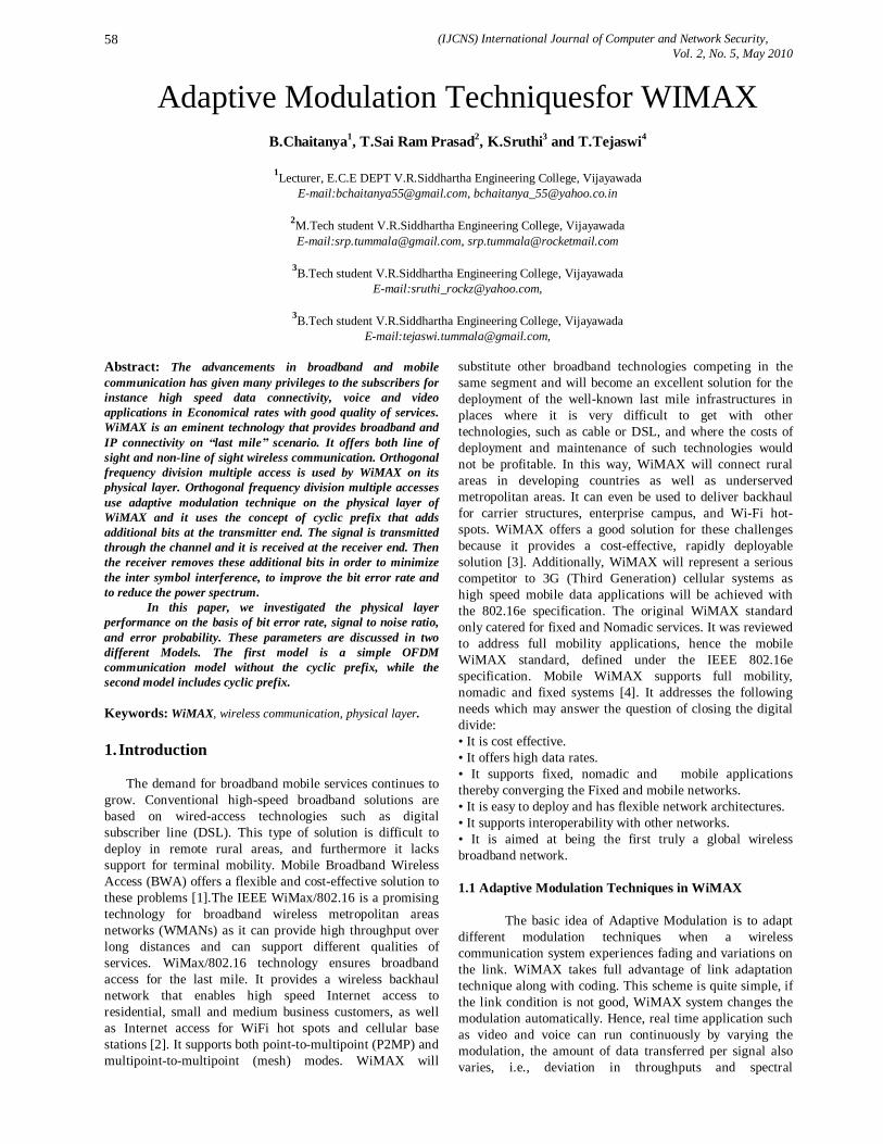
(IJCNS) International Journal of Computer and Network Security, Vol. 2, No. 5, May 2010
58
Adaptive Modulation Techniquesfor WIMAX
B.Chaitanya1, T.Sai Ram Prasad2, K.Sruthi3 and T.Tejaswi4
1Lecturer, E.C.E DEPT V.R.Siddhartha Engineering College, Vijayawada E-mail:[email protected], [email protected]
2M.Tech student V.R.Siddhartha Engineering College, Vijayawada
E-mail:[email protected], [email protected]
3B.Tech student V.R.Siddhartha Engineering College, Vijayawada E-mail:[email protected],
3B.Tech student V.R.Siddhartha Engineering College, Vijayawada
E-mail:[email protected],
Abstract: The advancements in broadband and mobile communication has given many privileges to the subscribers for instance high speed data connectivity, voice and video applications in Economical rates with good quality of services. WiMAX is an eminent technology that provides broadband and IP connectivity on “last mile” scenario. It offers both line of sight and non-line of sight wireless communication. Orthogonal frequency division multiple access is used by WiMAX on its physical layer. Orthogonal frequency division multiple accesses use adaptive modulation technique on the physical layer of WiMAX and it uses the concept of cyclic prefix that adds additional bits at the transmitter end. The signal is transmitted through the channel and it is received at the receiver end. Then the receiver removes these additional bits in order to minimize the inter symbol interference, to improve the bit error rate and to reduce the power spectrum. In this paper, we investigated the physical layer performance on the basis of bit error rate, signal to noise ratio, and error probability. These parameters are discussed in two different Models. The first model is a simple OFDM communication model without the cyclic prefix, while the second model includes cyclic prefix. Keywords: WiMAX, wireless communication, physical layer. 1. Introduction The demand for broadband mobile services continues to grow. Conventional high-speed broadband solutions are based on wired-access technologies such as digital subscriber line (DSL). This type of solution is difficult to deploy in remote rural areas, and furthermore it lacks support for terminal mobility. Mobile Broadband Wireless Access (BWA) offers a flexible and cost-effective solution to these problems [1].The IEEE WiMax/802.16 is a promising technology for broadband wireless metropolitan areas networks (WMANs) as it can provide high throughput over long distances and can support different qualities of services. WiMax/802.16 technology ensures broadband access for the last mile. It provides a wireless backhaul network that enables high speed Internet access to residential, small and medium business customers, as well as Internet access for WiFi hot spots and cellular base stations [2]. It supports both point-to-multipoint (P2MP) and multipoint-to-multipoint (mesh) modes. WiMAX will
substitute other broadband technologies competing in the same segment and will become an excellent solution for the deployment of the well-known last mile infrastructures in places where it is very difficult to get with other technologies, such as cable or DSL, and where the costs of deployment and maintenance of such technologies would not be profitable. In this way, WiMAX will connect rural areas in developing countries as well as underserved metropolitan areas. It can even be used to deliver backhaul for carrier structures, enterprise campus, and Wi-Fi hot-spots. WiMAX offers a good solution for these challenges because it provides a cost-effective, rapidly deployable solution [3]. Additionally, WiMAX will represent a serious competitor to 3G (Third Generation) cellular systems as high speed mobile data applications will be achieved with the 802.16e specification. The original WiMAX standard only catered for fixed and Nomadic services. It was reviewed to address full mobility applications, hence the mobile WiMAX standard, defined under the IEEE 802.16e specification. Mobile WiMAX supports full mobility, nomadic and fixed systems [4]. It addresses the following needs which may answer the question of closing the digital divide: • It is cost effective. • It offers high data rates. • It supports fixed, nomadic and mobile applications thereby converging the Fixed and mobile networks. • It is easy to deploy and has flexible network architectures. • It supports interoperability with other networks. • It is aimed at being the first truly a global wireless broadband network. 1.1 Adaptive Modulation Techniques in WiMAX The basic idea of Adaptive Modulation is to adapt different modulation techniques when a wireless communication system experiences fading and variations on the link. WiMAX takes full advantage of link adaptation technique along with coding. This scheme is quite simple, if the link condition is not good, WiMAX system changes the modulation automatically. Hence, real time application such as video and voice can run continuously by varying the modulation, the amount of data transferred per signal also varies, i.e., deviation in throughputs and spectral
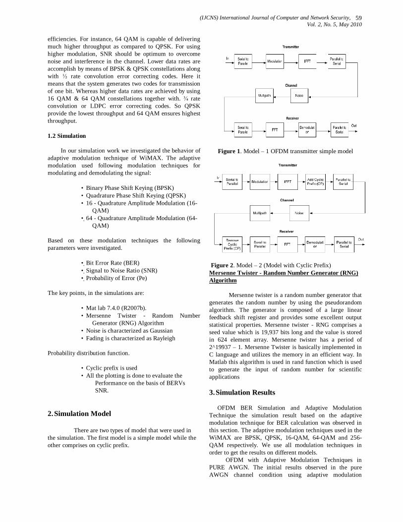
(IJCNS) International Journal of Computer and Network Security, Vol. 2, No. 5, May 2010
59
efficiencies. For instance, 64 QAM is capable of delivering much higher throughput as compared to QPSK. For using higher modulation, SNR should be optimum to overcome noise and interference in the channel. Lower data rates are accomplish by means of BPSK & QPSK constellations along with ½ rate convolution error correcting codes. Here it means that the system generates two codes for transmission of one bit. Whereas higher data rates are achieved by using 16 QAM & 64 QAM constellations together with. ¾ rate convolution or LDPC error correcting codes. So QPSK provide the lowest throughput and 64 QAM ensures highest throughput. 1.2 Simulation In our simulation work we investigated the behavior of adaptive modulation technique of WiMAX. The adaptive modulation used following modulation techniques for modulating and demodulating the signal:
• Binary Phase Shift Keying (BPSK) • Quadrature Phase Shift Keying (QPSK) • 16 - Quadrature Amplitude Modulation (16-
QAM) • 64 - Quadrature Amplitude Modulation (64-
QAM) Based on these modulation techniques the following parameters were investigated.
• Bit Error Rate (BER) • Signal to Noise Ratio (SNR) • Probability of Error (Pe)
The key points, in the simulations are:
• Mat lab 7.4.0 (R2007b). • Mersenne Twister - Random Number
Generator (RNG) Algorithm • Noise is characterized as Gaussian • Fading is characterized as Rayleigh
Probability distribution function.
• Cyclic prefix is used • All the plotting is done to evaluate the
Performance on the basis of BERVs SNR. 2. Simulation Model
There are two types of model that were used in the simulation. The first model is a simple model while the other comprises on cyclic prefix.
Figure 1. Model – 1 OFDM transmitter simple model
Figure 2. Model – 2 (Model with Cyclic Prefix) Mersenne Twister - Random Number Generator (RNG) Algorithm Mersenne twister is a random number generator that generates the random number by using the pseudorandom algorithm. The generator is composed of a large linear feedback shift register and provides some excellent output statistical properties. Mersenne twister - RNG comprises a seed value which is 19,937 bits long and the value is stored in 624 element array. Mersenne twister has a period of 2^19937 – 1. Mersenne Twister is basically implemented in C language and utilizes the memory in an efficient way. In Matlab this algorithm is used in rand function which is used to generate the input of random number for scientific applications 3. Simulation Results OFDM BER Simulation and Adaptive Modulation Technique the simulation result based on the adaptive modulation technique for BER calculation was observed in this section. The adaptive modulation techniques used in the WiMAX are BPSK, QPSK, 16-QAM, 64-QAM and 256-QAM respectively. We use all modulation techniques in order to get the results on different models. OFDM with Adaptive Modulation Techniques in PURE AWGN. The initial results observed in the pure AWGN channel condition using adaptive modulation
(IJCNS) International Journal of Computer and Network Security, Vol. 2, No. 5, May 2010
60
techniques and compared the performance of these techniques while using the 256 multicarrier OFDM waves.
Figure 3. OFDM with Adaptive Modulation Techniques in PURE AWGN
3.1 Theoretical Values of BER using Adaptive
Modulation Techniques in OFDM The theoretical value of BER with respect to adaptive modulation techniques in the presence of pure AWGN is used to estimate the theoretical value of SNR with 256 sub carriers
Figure 4. Theoretical Values of BER using Adaptive
Modulation Techniques in OFDM (CP) 3.2 OFDM with Adaptive Modulation Techniques in AWGN + Rayleigh Fading Channel with Cyclic Prefix There is another model which consists on AWGN and Rayleigh Fading Channel with the addition of Cyclic Prefix (CP) at the transmitter as well as receiver end. We investigate the effects of CP while using adaptive modulation techniques and compared the performance of OFDM symbols in terms of BER and SNR
Figure 5. OFDM with Adaptive Modulation Techniques in AWGN + Rayleigh Fading Channel with Cyclic Prefix (CP) 4. Probability of Error (Pe) for Adaptive
Modulation The Probability of Error (Pe) is the assumption of the rate of the error that introduce in the system because of noise and fading effects in the channel and also due to the cable losses at transmitter and the receiver ends. The Probability of Error for M-ary PSK has been calculated using the following formula:
Also for M-ary QAM the error probability given as:
Figure 6. Probability of Error (Pe) for Adaptive Modulation
5. Conclusion
We concluded that BPSK is more power efficient and need less bandwidth amongst all other modulation techniques used in an OFDM adaptive modulation. In case of bandwidth utilization the 64 and 256QAM modulation
(IJCNS) International Journal of Computer and Network Security, Vol. 2, No. 5, May 2010
61
requires higher bandwidth and gives an excellent data rates as compared to others. While the QPSK and the 16QAM techniques are in the middle of these two and need higher bandwidth and less power efficient than BPSK. But they required lesser bandwidth and lower data rates than 64QAM. Also, BPSK has the lowest BER while the 64-QAM has highest BER than others. There are other aspects as well that we conclude: 1 The inclusion of the Cyclic Prefix reduces the Inter Symbol Interference (ISI) that causes the lower BER in the OFDM system but increases the complexity of the system. 2. Model with CP requires high power as compared to the non-CP model. In future, adaptive modulation technique and OFDMA as physical layer will be adapted by Long Term Evaluation (LTE) and High Altitude Platform (HAP) References [1] Mai Tran, George Zaggoulos, Andrew Nix and Angela Doufexi,” Mobile WiMAX Performance Ana lysis and Comparison with Experimental Results” [2] J. El-Najjar, B. Jaumard, C.Assi, “Minimizing
Interference in WiMax/802.16 based Mesh Networks with Centralized Scheduling”, Global Telecommunications Conference, 2008. pp.1-6. http://www.intel.com/netcomms
/technologies/WiMAX/304471.pdf [3] Intel white paper, Wi-Fi and Wimax Solution: “Understanding Wi-Fi and Wimax as
Metro-Access Solution, “Intel Corporation 2004.
[4] A. Yarali, B. Mbula, A. Tumula, “WiMAX: A Key to Bridging the Digital Divide ”IEEE Volume, 2007, pp. 159 – 164. [5] WiMAX Forum, “Fixed, Nomadic, Portable and
Mobile Applications for 802.16-2004 and 802.16eWiMAXNetworks”, November,
2005. [6] T.TAN BENNY BING, "The World Wide Wi-
Fi: Technological Trends and B u s i n e s s Strategies", J O H N W I L E Y & S O N S , INC., 2003
[7] M. Nadeem Khan, S. Ghauri, “The WiMAX 802.16e Physical Layer Model”, IET
International Conference on Volume, 2008, pp.117 – 120.
[8] Kavesh Pahlavan and prashant Krishna Murthy “Principles of Wireless Network “Prentice-Hall, Inc., 2006 [9] Yango Xiao, “Wimax/Mobile”MobileFi Advanced Research and Technology Auerbach publications, 2008.
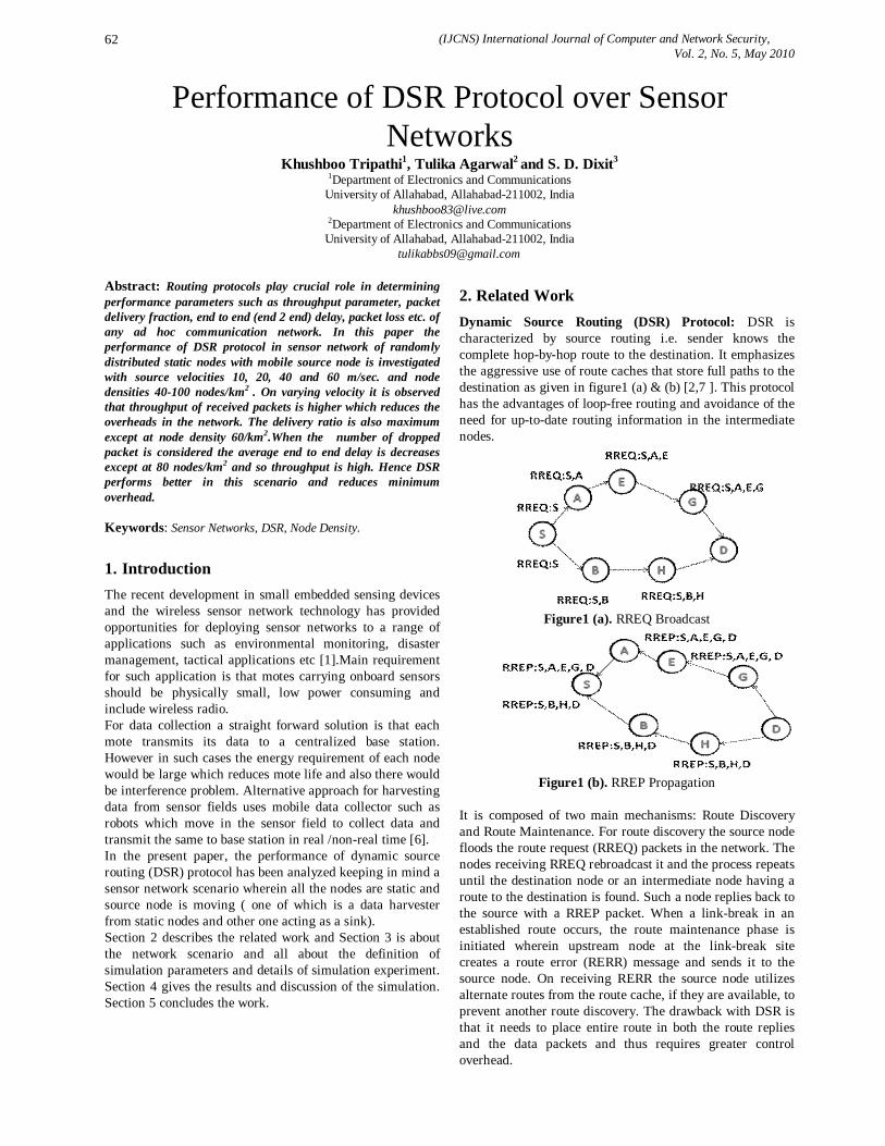
(IJCNS) International Journal of Computer and Network Security, Vol. 2, No. 5, May 2010
62
Performance of DSR Protocol over Sensor Networks
Khushboo Tripathi1, Tulika Agarwal2 and S. D. Dixit3 1Department of Electronics and Communications University of Allahabad, Allahabad-211002, India
[email protected] 2Department of Electronics and Communications University of Allahabad, Allahabad-211002, India
Abstract: Routing protocols play crucial role in determining performance parameters such as throughput parameter, packet delivery fraction, end to end (end 2 end) delay, packet loss etc. of any ad hoc communication network. In this paper the performance of DSR protocol in sensor network of randomly distributed static nodes with mobile source node is investigated with source velocities 10, 20, 40 and 60 m/sec. and node densities 40-100 nodes/km2 . On varying velocity it is observed that throughput of received packets is higher which reduces the overheads in the network. The delivery ratio is also maximum except at node density 60/km2.When the number of dropped packet is considered the average end to end delay is decreases except at 80 nodes/km2 and so throughput is high. Hence DSR performs better in this scenario and reduces minimum overhead. Keywords: Sensor Networks, DSR, Node Density.
1. Introduction
The recent development in small embedded sensing devices and the wireless sensor network technology has provided opportunities for deploying sensor networks to a range of applications such as environmental monitoring, disaster management, tactical applications etc [1].Main requirement for such application is that motes carrying onboard sensors should be physically small, low power consuming and include wireless radio. For data collection a straight forward solution is that each mote transmits its data to a centralized base station. However in such cases the energy requirement of each node would be large which reduces mote life and also there would be interference problem. Alternative approach for harvesting data from sensor fields uses mobile data collector such as robots which move in the sensor field to collect data and transmit the same to base station in real /non-real time [6]. In the present paper, the performance of dynamic source routing (DSR) protocol has been analyzed keeping in mind a sensor network scenario wherein all the nodes are static and source node is moving ( one of which is a data harvester from static nodes and other one acting as a sink). Section 2 describes the related work and Section 3 is about the network scenario and all about the definition of simulation parameters and details of simulation experiment. Section 4 gives the results and discussion of the simulation. Section 5 concludes the work.
2. Related Work Dynamic Source Routing (DSR) Protocol: DSR is characterized by source routing i.e. sender knows the complete hop-by-hop route to the destination. It emphasizes the aggressive use of route caches that store full paths to the destination as given in figure1 (a) & (b) [2,7 ]. This protocol has the advantages of loop-free routing and avoidance of the need for up-to-date routing information in the intermediate nodes.
Figure1 (a). RREQ Broadcast
Figure1 (b). RREP Propagation
It is composed of two main mechanisms: Route Discovery and Route Maintenance. For route discovery the source node floods the route request (RREQ) packets in the network. The nodes receiving RREQ rebroadcast it and the process repeats until the destination node or an intermediate node having a route to the destination is found. Such a node replies back to the source with a RREP packet. When a link-break in an established route occurs, the route maintenance phase is initiated wherein upstream node at the link-break site creates a route error (RERR) message and sends it to the source node. On receiving RERR the source node utilizes alternate routes from the route cache, if they are available, to prevent another route discovery. The drawback with DSR is that it needs to place entire route in both the route replies and the data packets and thus requires greater control overhead.

(IJCNS) International Journal of Computer and Network Security, Vol. 2, No. 5, May 2010
63
3. Network Scenario and Simulation Details The simulation scenario consists of tcl script that runs over TCP connections for various number of nodes (40, 60, 80 and of 100 nodes) in an area of size of 1000 1000m2. Figure 2 shows the random node topology of the network. The simulation time is set to 150 seconds. TCP connection has been used to set communication between the source node and the sink node.
Figure 2. NAM Windows showing network topology for
100 nodes The simulation is carried out in the network simulator NS-2 (version-2.31) over LINUX (FEDORA 8) environment [3] [4].The experiment has been performed for a set of 5 random network topologies having number of nodes 40,60,80 and 100 respectively. In each topology all nodes are fixed except the source node. For a given topology two nodes are selected to be source-sink nodes and the observations are made for five different velocities 10, 20, 40 and 60 m/sec. The experiment was repeated by selecting another pairs of source-sink nodes chosen randomly. Five such observations were taken for each of the following three performance parameters and their averages are obtained to plot graphs: 1. Bytes Delivery Fraction: The ratio of the number of data sends (in bytes) successfully delivered to the destinations to those are generated by TCP agents/sources. Thus, Bytes Delivery Fraction = (Received data /Total sent data) 2. Average Number of Dropped Packets: This parameter is worth mentioning while taking the effectiveness of this routing protocol. These are the average number of dropped packets in simulation study of our scenario. 3. Average Simulation End to End Delay: The delivery delay for the data is the interval between when it is generated at a sensor node and when it is collected by a sink [2]. It does not depend on the time for collecting data from the network. These are the possible delays caused by buffering during route discovery latency, queuing at the interface queue, retransmission delays at the MAC and propagation and transfer times. Simulation Parameters: The parameter values for simulation are given in table 1.
Table1: Parameter values for simulation
Maximum simulation time
150 seconds
Area size (Flat area) 1000×1000 m2 Routing protocol (proactive)
DSR
Propagation Model Two Ray Ground Propagation
MAC layers protocol IEEE802.11 Node placement Static Random
Distribution Number of nodes 40,60,80,100 Velocities of source and sink nodes
10,20,40,60 m/sec
4. Results and Discussion The throughput vs. node density graph is given in figure3. According to our topology considerations, in sparse network, for the velocities 10, 20, 40 and 60 m/sec different throughput graphs are obtained. For all the velocities at the node density 60 per square km minimum throughput is obtained while higher velocities give maximum throughput with node density parameter. At velocity 10m/sec throughput is minimum whereas at velocity 60 m/sec throughput is higher in comparison to other velocities. This is because of the nature of DSR on-demand routing protocol. Once the route is formed the possibility of (link-breakage) is lesser as compared to the former case where the probability of route formation is lower. Hence it is clear from figure after node density 60 per square km throughput is generally increasing in nature with different node densities due to less link breakage in route formation. It is obtained that When the throughput of received packets is maximum the number of overheads reduces in the network.
40 50 60 70 80 90 1003000
3500
4000
4500
5000
5500
6000
Node Density(per square km)
Thro
ughp
ut
nv10nv20nv40nv60
Figure3.Throughput (of received packets) vs. node density
The packet delivery fraction vs. node density behavior is given in figure 4. We have seen the effect of delivery ratio with node density on varying the velocities 10, 20, 40 and 60 m/sec. The delivery fraction graph is almost similar to the throughput vs. node density figure. On varying node density the delivery fraction is increased for all the velocities except at node density 60 per square km.
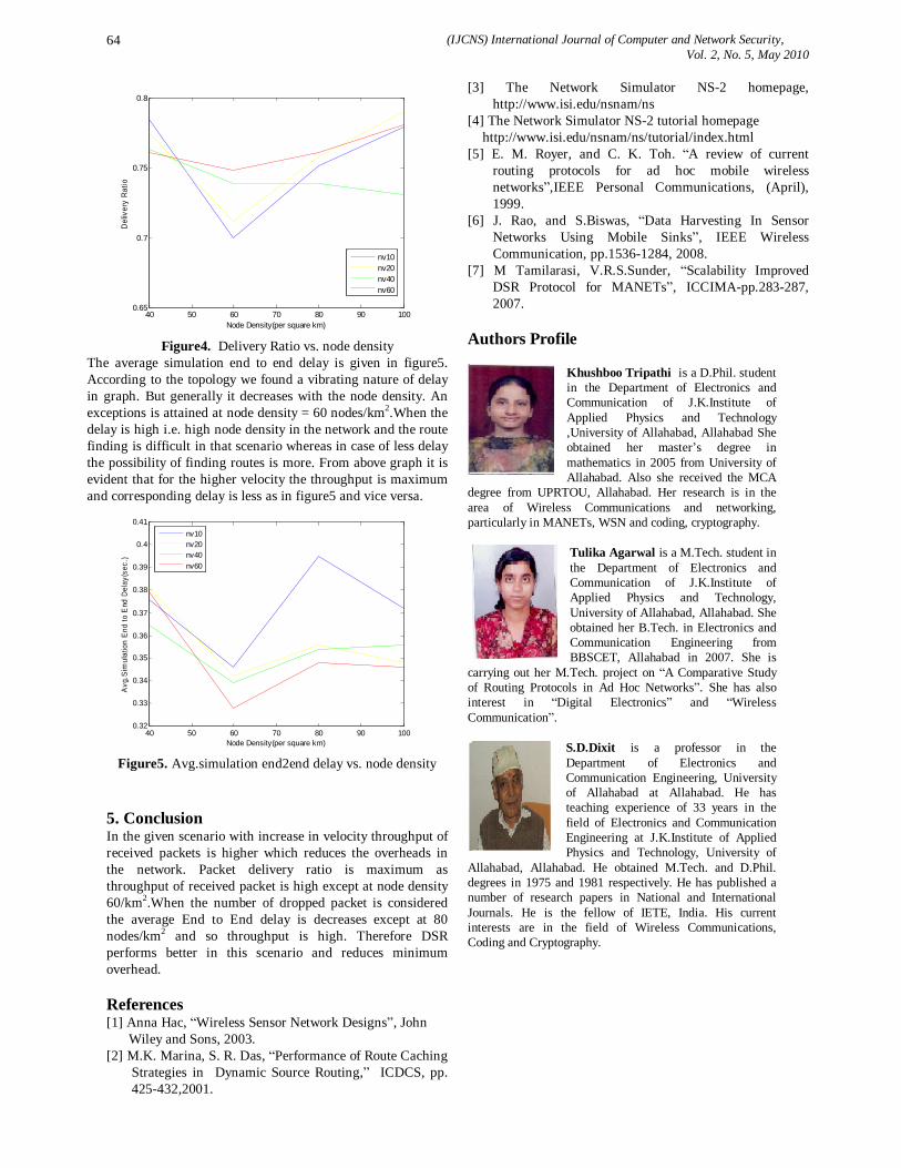
(IJCNS) International Journal of Computer and Network Security, Vol. 2, No. 5, May 2010
64
40 50 60 70 80 90 1000.65
0.7
0.75
0.8
Node Density(per square km)
Del
iver
y Ra
tio
nv10nv20nv40nv60
Figure4. Delivery Ratio vs. node density
The average simulation end to end delay is given in figure5. According to the topology we found a vibrating nature of delay in graph. But generally it decreases with the node density. An exceptions is attained at node density = 60 nodes/km2.When the delay is high i.e. high node density in the network and the route finding is difficult in that scenario whereas in case of less delay the possibility of finding routes is more. From above graph it is evident that for the higher velocity the throughput is maximum and corresponding delay is less as in figure5 and vice versa.
40 50 60 70 80 90 1000.32
0.33
0.34
0.35
0.36
0.37
0.38
0.39
0.4
0.41
Node Density(per square km)
Avg
.Sim
ulat
ion
End
to E
nd D
elay
(sec
.)
nv10nv20nv40nv60
Figure5. Avg.simulation end2end delay vs. node density
5. Conclusion In the given scenario with increase in velocity throughput of received packets is higher which reduces the overheads in the network. Packet delivery ratio is maximum as throughput of received packet is high except at node density 60/km2.When the number of dropped packet is considered the average End to End delay is decreases except at 80 nodes/km2 and so throughput is high. Therefore DSR performs better in this scenario and reduces minimum overhead.
References [1] Anna Hac, “Wireless Sensor Network Designs”, John Wiley and Sons, 2003. [2] M.K. Marina, S. R. Das, “Performance of Route Caching
Strategies in Dynamic Source Routing,” ICDCS, pp. 425-432,2001.
[3] The Network Simulator NS-2 homepage, http://www.isi.edu/nsnam/ns
[4] The Network Simulator NS-2 tutorial homepage http://www.isi.edu/nsnam/ns/tutorial/index.html [5] E. M. Royer, and C. K. Toh. “A review of current
routing protocols for ad hoc mobile wireless networks”,IEEE Personal Communications, (April), 1999.
[6] J. Rao, and S.Biswas, “Data Harvesting In Sensor Networks Using Mobile Sinks”, IEEE Wireless Communication, pp.1536-1284, 2008.
[7] M Tamilarasi, V.R.S.Sunder, “Scalability Improved DSR Protocol for MANETs”, ICCIMA-pp.283-287, 2007.
Authors Profile
Khushboo Tripathi is a D.Phil. student in the Department of Electronics and Communication of J.K.Institute of Applied Physics and Technology ,University of Allahabad, Allahabad She obtained her master’s degree in mathematics in 2005 from University of Allahabad. Also she received the MCA
degree from UPRTOU, Allahabad. Her research is in the area of Wireless Communications and networking, particularly in MANETs, WSN and coding, cryptography.
Tulika Agarwal is a M.Tech. student in the Department of Electronics and Communication of J.K.Institute of Applied Physics and Technology, University of Allahabad, Allahabad. She obtained her B.Tech. in Electronics and Communication Engineering from BBSCET, Allahabad in 2007. She is
carrying out her M.Tech. project on “A Comparative Study of Routing Protocols in Ad Hoc Networks”. She has also interest in “Digital Electronics” and “Wireless Communication”.
S.D.Dixit is a professor in the Department of Electronics and Communication Engineering, University of Allahabad at Allahabad. He has teaching experience of 33 years in the field of Electronics and Communication Engineering at J.K.Institute of Applied Physics and Technology, University of
Allahabad, Allahabad. He obtained M.Tech. and D.Phil. degrees in 1975 and 1981 respectively. He has published a number of research papers in National and International Journals. He is the fellow of IETE, India. His current interests are in the field of Wireless Communications, Coding and Cryptography.

(IJCNS) International Journal of Computer and Network Security, Vol. 2, No. 5, May 2010
65
Route Information Update in Mobile Ad Hoc Networks
Seungjin Park1 and Seong-Moo Yoo2
1University of Southern Indiana, Department of Management, MIS & CS,
8600 University Blvd., Evansville, IN 47712, USA [email protected]
2The University of Alabama in Huntsville, Electrical & Computer Engineering Department,
301 Sparkman Dr., Huntsville, AL 35899, USA [email protected]
Abstract: A mobile ad hoc network (MANET) is composed of moving wireless hosts that, within range of each other, form wireless networks. For communication to occur between hosts that are not within each other’s range, routes involving intermediate nodes should be established. However, due to the mobility of the nodes, finding routes in a MANET is quite a challenging task, and takes up a lot of system resources such as bandwidth and battery power. Although it would be wise to take full advantage of the already discovered paths, many algorithms simply discard the paths if their topology has changed. To overcome this shortcoming, we have proposed a routing table maintenance algorithm that responds to the changes in network topology promptly, and adjusts the paths so that their lifetimes could be maximized.
Keywords: mobile ad hoc network, routing, routing table, unicast
1. Introduction A mobile ad hoc network (MANET) consists of wireless mobile hosts without any centralized control point or fixed infrastructure. Since a MANET does not require any prior arrangement, it can be quickly deployed and used in such applications including fast establishment of military communication and rescue missions where an established network is neither feasible nor available [1].
Discovering a path from the source node to the destination node is quite challenging in a MANET due to the mobility of hosts. A node implementing a proactive algorithm [2] maintains a routing table that contains the routes to all nodes in the network by periodical exchanges of local information with other nodes. However, this information exchange takes up a lot of bandwidth and battery power. On the other hand, nodes in reactive algorithms [3, 4, 5] do not maintain any routing information. Instead, a node dynamically discovers a path to the destination on demand. Therefore, it may reduce considerable overhead to enhance the network throughput. Although other routing algorithm could be used, this paper is based on DSR [5]. DSR is reactive and has been proved it could be as competitive as any other algorithms in MANET [7, 8, 9]. Like many reactive routing protocol, DSR consists of two phases: route discovery phase and data delivery phase. When node S has a data for node D, S starts finding a path to D in the route discovery phase. Once a route is
found, S sends data along the path in the data delivery phase. In the route discovery phase S broadcasts a control packet called a route request packet (REQ) to all its neighbor nodes. If a neighbor node does not have route information to D, it appends its information to the REQ and relays the REQ to all its neighbor nodes, and so on until the REQ reaches D. (This forwarding of requests from one node to all its neighbors is called “flooding” and consumes a lot of time and bandwidth.) If the REQ reaches either D or a node that contains the path information to D, the node sends a control packet called route reply packet (RPY) back to S by reversing the path stored in the REQ.
On receiving the RPY, S knows that the path to D has been established, and S sends its data packet along the path. For example, suppose node A in Figure 1 tries to find a path to G that is not found yet. As a first step, A prepares an REQ with its ID appended to it, and sends it to its neighbors including B. If B does not have any information about G, B appends its ID to the REQ and retransmits it to its neighbors including C, and so on until it reaches G. The snapshot of the REQ at E would contain the nodes it passed through thus far, which is A, B, C, D. When the REQ reaches the destination node G, G prepares a RPY which is transmitted to A along the path stored in the REQ.
A
B C
D E
F G
I H
Figure 1. There are two paths, P(A, B, C, D, E, F, G) and
P(H, I, C, D, E, F, G) in the networks.
For example, on receiving the RPY, node A in Figure 1 stores the path (A, B, C, D, E, F, G), and node C stores the path (C, D, E, F, G) in their routing tables so that they can use it later. As mentioned before, it takes a lot of resources to discover a path in a MANET. Therefore, it would be wise to take advantage of it as much as possible. However, most routing protocols do not efficiently utilize the existing paths, because they do not respond properly and promptly to the changes in the network topology. In this paper, we propose a strategy that tries to use the existing paths
(IJCNS) International Journal of Computer and Network Security, Vol. 2, No. 5, May 2010
66
efficiently by modifying route table as quickly as possible. This paper is organized as follows. Previous work is mentioned in section 2. Terminology needed to understand this paper is explained in section 3. Proposed algorithm is presented in section 4, followed by the theoretical analysis in section 5. Section 6 presents the conclusion.
2. Previous Works Wu et al. [6] proposed an algorithm that tries to fix some problems in paths such as finding shorter paths and fixing broken links. However, nodes in their algorithm stores only the destination, next hop, hop count, etc. for each path so that the coverage of the algorithm is limited. Ko and Vaidya [10] proposed a location-aided routing scheme where a route request is flooded in the direction of the target node. Here, a node’s response to the route request depends on whether or not it is in the region approaching the destination. Liao et al. [11] proposed a routing scheme called GRID. This scheme imposes a grid system on the earth’s surface and selects a leader in each grid to act as the gateway. Data packets are then forwarded to their destination grid by grid. This protocol confirms that the availability of location information improves the routing performance.
Lee and Gerla [12] proposed AODV-BR algorithm that utilizes a mesh structure to provide multiple alternate paths to existing on-demand routing protocols without producing additional control messages. In their algorithm, data packets are delivered through the primary route unless there is a route disconnection. When a node detects a link break, data packets can be delivered through one or more alternate routes and are not dropped. Route maintenance is executed utilizing alternate paths. Here, the route is maintained only when a link is broken.
Li and Mohapatra [13] introduced LAKER, a location-aided knowledge extraction routing. This scheme reduces the flooding overhead in route discovery by extracting knowledge of the nodal density distribution of the network and remembering the series of locations along the route where there are many nodes around. However, this scheme does not deal with route maintenance.
Stoimenovic [14] reviewed many position-based routings in ad hoc networks. It is likely that only position-based approaches provide satisfactory performance for large networks. Greedy mode routing was shown to nearly guarantee delivery for dense graphs, but to fail frequently for sparse graphs since the destination is also moving and it is not clear where to send message. The routing process is converted from the greedy mode to recovery mode at a node where greedy mode fails to advance a message toward the destination
Park et al. [15] proposed an anticipated route maintenance protocol with two extensions to route discovery based routing scheme: extending a route by inserting a common neighbor of two nodes in a route when the two nodes move apart from each other that may cause link breakage, and
shrinking a route when a node discovers a shorter path than the existing one. By utilizing only local geographic information, a host can anticipate its neighbor’s departure and, if other hosts are available, choose a host to bridge the gap, keeping the path connected. The benefits are that this reduces the need to find new routes and prevents interruptions in service.
Chou et al. [16] presented a dynamic route maintenance algorithm for beacon-based geographic routing. In this approach, the mobile nodes dynamically adjust their beacon intervals based on their speed of movement. Moreover the routing information could be well managed using the mobility prediction.
Park et al. [17] proposed an algorithm that is a preliminary version of the paper. However, the algorithm presented in this paper considers more cases that may save more battery power and bandwidth.
3. Terminology A Graph can be represented by G(V, E), where V is the set of nodes and E is the set of links in the graph G. In a wireless network, if a node B is within the transmission range of node A, then it is said that there is a link from A to B which is denoted as (A, B). A is an upstream node of B, and B is the downstream node of A. B is also called as a neighbor of A. If (A, B) implies (B, A), then the link is called bidirectional, and unidirectional otherwise. A path P(v1, v2, . . . , vn-1, vn), where vi ∈ V, 1 ≤ i ≤ n, consists of a set of links (v1, v2), (v2, v3), … , (vn-1, vn). A subpath of P(v1, v2, . . . , vn-1, vn) is the path that is a part of P. Function rem (P, vi) returns the portion of path P starting at node vi to the end of P. For example, both P(B, C, D, E) and P(A, B) are subpaths of P(A, B, C, D, E), and rem (P(A, B, C, D, E), B) is P(B, C, D, E). |P| denotes the number of the links in path P. For example, |P(A, B, C, D, E)| is four, since P consists of four links. Note that if the links are bidirectional (unidirectional, resp.), then the paths are also bidirectional (unidirectional, resp.). Although links assumed to be bidirectional in this paper, paths are assumed to be unidirectional for simplicity in explanation. It can be easily extended to cover the handling of unidirectional paths. When a new path is found, each node in the path may contain the path information in its Routing Table for possible later use. This can be done without any extra expense at each node by simply storing the path information when the RPY passes through the node. For example in Figure 1, nodes A, B, C, D, E, and F in the path P(A, B, C, D, E, F, G) store the path information when the RPY passes through them.
4. Proposed Routing Table Maintenance Scheme
Based on the assumption that all links are bidirectional, the proposed scheme is hybrid, since it discovers new paths
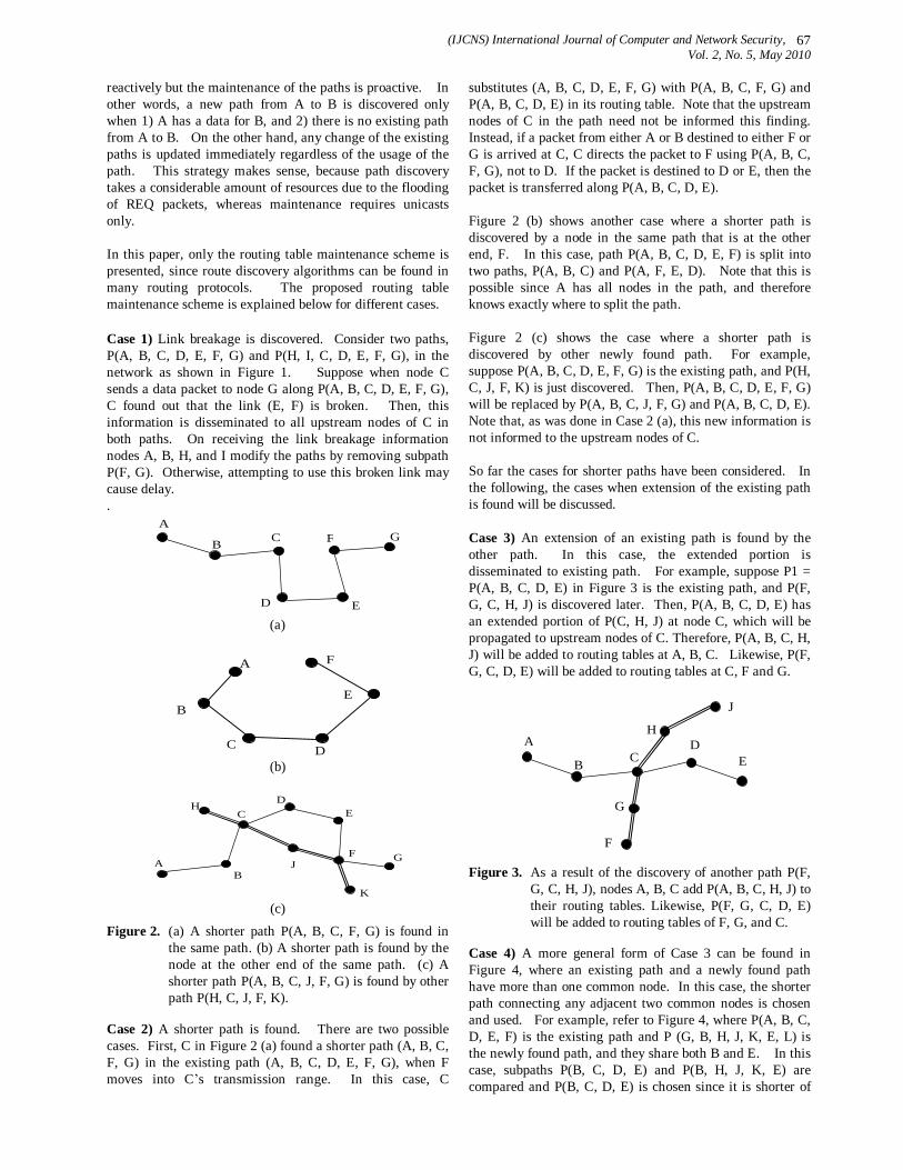
(IJCNS) International Journal of Computer and Network Security, Vol. 2, No. 5, May 2010
67
reactively but the maintenance of the paths is proactive. In other words, a new path from A to B is discovered only when 1) A has a data for B, and 2) there is no existing path from A to B. On the other hand, any change of the existing paths is updated immediately regardless of the usage of the path. This strategy makes sense, because path discovery takes a considerable amount of resources due to the flooding of REQ packets, whereas maintenance requires unicasts only. In this paper, only the routing table maintenance scheme is presented, since route discovery algorithms can be found in many routing protocols. The proposed routing table maintenance scheme is explained below for different cases. Case 1) Link breakage is discovered. Consider two paths, P(A, B, C, D, E, F, G) and P(H, I, C, D, E, F, G), in the network as shown in Figure 1. Suppose when node C sends a data packet to node G along P(A, B, C, D, E, F, G), C found out that the link (E, F) is broken. Then, this information is disseminated to all upstream nodes of C in both paths. On receiving the link breakage information nodes A, B, H, and I modify the paths by removing subpath P(F, G). Otherwise, attempting to use this broken link may cause delay. .
A
B C
D E
F G
(a)
A
B
C D
E
F
(b)
A B
C E
F G
H
J
K
D
(c)
Figure 2. (a) A shorter path P(A, B, C, F, G) is found in the same path. (b) A shorter path is found by the node at the other end of the same path. (c) A shorter path P(A, B, C, J, F, G) is found by other path P(H, C, J, F, K).
Case 2) A shorter path is found. There are two possible cases. First, C in Figure 2 (a) found a shorter path (A, B, C, F, G) in the existing path (A, B, C, D, E, F, G), when F moves into C’s transmission range. In this case, C
substitutes (A, B, C, D, E, F, G) with P(A, B, C, F, G) and P(A, B, C, D, E) in its routing table. Note that the upstream nodes of C in the path need not be informed this finding. Instead, if a packet from either A or B destined to either F or G is arrived at C, C directs the packet to F using P(A, B, C, F, G), not to D. If the packet is destined to D or E, then the packet is transferred along P(A, B, C, D, E). Figure 2 (b) shows another case where a shorter path is discovered by a node in the same path that is at the other end, F. In this case, path P(A, B, C, D, E, F) is split into two paths, P(A, B, C) and P(A, F, E, D). Note that this is possible since A has all nodes in the path, and therefore knows exactly where to split the path. Figure 2 (c) shows the case where a shorter path is discovered by other newly found path. For example, suppose P(A, B, C, D, E, F, G) is the existing path, and P(H, C, J, F, K) is just discovered. Then, P(A, B, C, D, E, F, G) will be replaced by P(A, B, C, J, F, G) and P(A, B, C, D, E). Note that, as was done in Case 2 (a), this new information is not informed to the upstream nodes of C. So far the cases for shorter paths have been considered. In the following, the cases when extension of the existing path is found will be discussed. Case 3) An extension of an existing path is found by the other path. In this case, the extended portion is disseminated to existing path. For example, suppose P1 = P(A, B, C, D, E) in Figure 3 is the existing path, and P(F, G, C, H, J) is discovered later. Then, P(A, B, C, D, E) has an extended portion of P(C, H, J) at node C, which will be propagated to upstream nodes of C. Therefore, P(A, B, C, H, J) will be added to routing tables at A, B, C. Likewise, P(F, G, C, D, E) will be added to routing tables at C, F and G.
A
B C D
E
F
G
H
J
Figure 3. As a result of the discovery of another path P(F,
G, C, H, J), nodes A, B, C add P(A, B, C, H, J) to their routing tables. Likewise, P(F, G, C, D, E) will be added to routing tables of F, G, and C.
Case 4) A more general form of Case 3 can be found in Figure 4, where an existing path and a newly found path have more than one common node. In this case, the shorter path connecting any adjacent two common nodes is chosen and used. For example, refer to Figure 4, where P(A, B, C, D, E, F) is the existing path and P (G, B, H, J, K, E, L) is the newly found path, and they share both B and E. In this case, subpaths P(B, C, D, E) and P(B, H, J, K, E) are compared and P(B, C, D, E) is chosen since it is shorter of
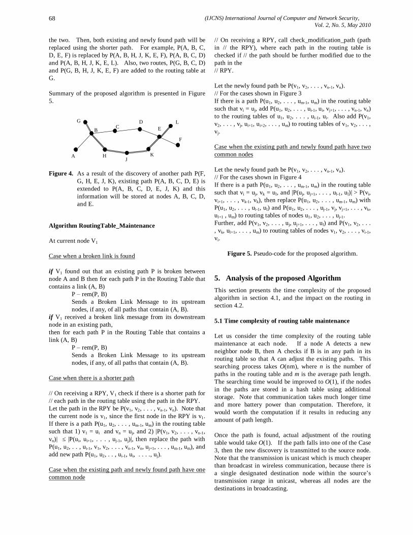
(IJCNS) International Journal of Computer and Network Security, Vol. 2, No. 5, May 2010
68
the two. Then, both existing and newly found path will be replaced using the shorter path. For example, P(A, B, C, D, E, F) is replaced by P(A, B, H, J, K, E, F), P(A, B, C, D) and P(A, B, H, J, K, E, L). Also, two routes, P(G, B, C, D) and P(G, B, H, J, K, E, F) are added to the routing table at G. Summary of the proposed algorithm is presented in Figure 5.
A
B C D
E
F
G
H J
K
L
Figure 4. As a result of the discovery of another path P(F,
G, H, E, J, K), existing path P(A, B, C, D, E) is extended to P(A, B, C, D, E, J, K) and this information will be stored at nodes A, B, C, D, and E.
Algorithm RoutingTable_Maintenance At current node V1 Case when a broken link is found if V1 found out that an existing path P is broken between node A and B then for each path P in the Routing Table that contains a link (A, B)
P – rem(P, B) Sends a Broken Link Message to its upstream nodes, if any, of all paths that contain (A, B).
if V1 received a broken link message from its downstream node in an existing path, then for each path P in the Routing Table that contains a link (A, B)
P – rem(P, B) Sends a Broken Link Message to its upstream nodes, if any, of all paths that contain (A, B).
Case when there is a shorter path // On receiving a RPY, V1 check if there is a shorter path for // each path in the routing table using the path in the RPY. Let the path in the RPY be P(v1, v2, . . . , vn-1, vn). Note that the current node is v1, since the first node in the RPY is v1. If there is a path P(u1, u2, . . . , um-1, um) in the routing table such that 1) v1 = ui and vn = uj, and 2) |P(v1, v2, . . . , vn-1, vn)| ≤ |P(ui, ui+1, . . . , uj-1, uj)|, then replace the path with P(u1, u2, . . , ui-1, v1, v2, . . . , vn-1, vn, uj+1, . . . , um-1, um), and add new path P(u1, u2, . . , ui-1, ui, . . . ., uj). Case when the existing path and newly found path have one common node
// On receiving a RPY, call check_modification_path (path in // the RPY), where each path in the routing table is checked if // the path should be further modified due to the path in the // RPY. Let the newly found path be P(v1, v2, . . . , vn-1, vn). // For the cases shown in Figure 3 If there is a path P(u1, u2, . . . , um-1, um) in the routing table such that vi = uj, add P(u1, u2, . . . , ui-1, ui, vj+1, . . . , vn-1, vn) to the routing tables of u1, u2, . . . , ui-1, ui. Also add P(v1, v2, . . . , vj, ui+1, ui+2, . . . , um) to routing tables of v1, v2, . . . , vj. Case when the existing path and newly found path have two common nodes Let the newly found path be P(v1, v2, . . . , vn-1, vn). // For the cases shown in Figure 4 If there is a path P(u1, u2, . . . , um-1, um) in the routing table such that vi = uj, vk = ul, and |P(uj, uj+1, . . . , ul-1, ul)| > P(vi, vi+1, . . . , vk-1, vk), then replace P(u1, u2, . . . , um-1, um) with P(u1, u2, . . . , ul-1, ul) and P(u1, u2, . . . , uj-1, vj, vj+1, . . . , vk, ul+1 , um) to routing tables of nodes u1, u2, . . . , uj-1. Further, add P(v1, v2, . . . , uj, uj+1, . . . , ul) and P(v1, v2, . . . , vk, ul+1, . . . , um) to routing tables of nodes v1, v2, . . . , vi-1, vi.
Figure 5. Pseudo-code for the proposed algorithm.
5. Analysis of the proposed Algorithm This section presents the time complexity of the proposed algorithm in section 4.1, and the impact on the routing in section 4.2. 5.1 Time complexity of routing table maintenance Let us consider the time complexity of the routing table maintenance at each node. If a node A detects a new neighbor node B, then A checks if B is in any path in its routing table so that A can adjust the existing paths. This searching process takes O(nm), where n is the number of paths in the routing table and m is the average path length. The searching time would be improved to O(1), if the nodes in the paths are stored in a hash table using additional storage. Note that communication takes much longer time and more battery power than computation. Therefore, it would worth the computation if it results in reducing any amount of path length. Once the path is found, actual adjustment of the routing table would take O(1). If the path falls into one of the Case 3, then the new discovery is transmitted to the source node. Note that the transmission is unicast which is much cheaper than broadcast in wireless communication, because there is a single designated destination node within the source’s transmission range in unicast, whereas all nodes are the destinations in broadcasting.

(IJCNS) International Journal of Computer and Network Security, Vol. 2, No. 5, May 2010
69
5.2 Impact on route discovery This section presents the theoretical analysis of the proposed algorithm to show how our proposed algorithm can reduce communication overhead and battery power by modifying routing tables on discovering a new path. Suppose N is the average number of neighbors of each node in the network. If an algorithm abandons the path on its topological changes, then it would take at least
110 ... −⋅⋅⋅ LNNN ≈ N2L REQ transmissions to find a path of length L all over again by using broadcast. On the other hand, if an algorithm can adjust to the minor topological changes of paths like our proposed algorithm, then it would take only L transmissions for the path of length L. Therefore, the advantage of having the proposed algorithm is obvious. This analysis would be true, if the changed path is used, otherwise, the adjustment would be a waste.
6. Conclusion Routing in a wireless mobile ad hoc network is quite a challenging task, because it takes up a lot of network resources. Therefore, although it would be wise to take full advantage of the already discovered paths, many algorithms simply discard the paths when their topology is changed. To overcome this shortcoming, we have proposed a routing table maintenance algorithm that responds to the changes in network topology as promptly yet efficiently as possible to fully utilize existing paths by modifying them. Our simple analysis shows that the proposed algorithm reduces number of packet transmissions, and therefore saves resources such as bandwidth and battery power.
References [1] C. Perkins, “Ad Hoc Networking,” Addison-Wesley,
2001. [2] C. Perkins, and P. Bhagwat, “Highly-dynamic
destination-sequenced distance-vector routing (DSDV) for mobile computers,” pp. 234-244, SIGCOM’94, 1994.
[3] C. Perkins, E. Royer and S. Das, “Ad hoc on demand distance vector (AODV) routing,” Internet draft, IETF, Oct. 1999.
[4] V. Park and M. Corson, “A highly adaptive distributed routing algorithm for mobile wireless networks,” In Proc. IEEE Infocom, pp.1405-1413, Apr. 1997
[5] D. Johnson and D. Maltz, “Dynamic source routing in ad-hoc wireless networking,” in Mobile Computing, T. Imielinski and H. Korth, editors Kluwer Academic Publishing, 1996.
[6] S. Wu, S. Ni, Y. Tseng, and J. Sheu, “Route maintenance in a wireless mobile ad hoc network,” Proc. 33 Hawaii International Conference on System Sciences, 2000.
[7] J. Broch, D. Maltz, D. Johnson, Y. Hu, and J. Jetcheva, “Performance comparison of multi-hop wireless ad hoc network routing protocols,” MobiCom’98, 1998.
[8] A. Rahman, S. Islam, and A. Talevski, “Performance measurement of various routing protocols in ad-hoc network,” Proc. International Multiconference of Engineers and Computer Scientists, 2009.
[9] G. Jayakumar and G. Gopinath, “Performance Comparison of two on-demand routing protocols for ad-choc networks based on random way point mobility model,” American Journal of Applied Sciences, 5 (6), pp. 659 – 664, 2008.
[10] Y. B. Ko and N.H. Vaidya, “Location-aided routng (LAR) in mobile ad hoc networks,” Annual International Conference on Mobile Computing and Networking (MobiCom), Oct. 1998, pp. 66-75.
[11] W.H. Liao, Y.C. Tseng, and J.P. Sheu, “GRID: a fully location-aware routing protocol for mobile ad hoc networks,” Telcommunication Systems, 18(13), 2001, pp. 37-60.
[12] S.J. Lee and M. Gerla, "AODV-BR: backup routing in ad hoc networks", IEEE Wireless Communications and Networking Conference (WCNC), Sept. 2000, pp. 1311–1316.
[13] Jian Li and P. Mohapatra, "LAKER: location aided knowledge extraction routing for mobile ad hoc networks", IEEE Wireless Communications and Networking (WCNC), March 2003, pp. 1180–1184.
[14] I. Stojmenovic, “Position-based routing in ad hoc networks,” IEEE Communications Magazine, July 2002, pp. 2-8.
[15] S. Park, S.M. Yoo, M. Al-Shurman, B. VanVoorst, and C.H. Jo, “ARM: anticipated route maintenance scheme in location-aided mobile ad hoc networks,” Journal of Communications and Networks, vol. 7, no. 3, pp. 325-336, Sep. 2005.
[16] C.H. Chou, K.F. Ssu, and H.C. Jiau, “Dynamic route maintenance for geographic forwarding in mobile ad hoc networks,” Computer Networks, vol. 52, issue 2, pp. 418-431, Feb. 2008.
[17] S. Park and S. Yoo, Routing table Maintenance in Mobile Ad Hoc Networks, The 12th International Conference on Advanced Communication Technology, pp. 1321 - 1325, Feb., 2010.
Authors Profile Seungjin Park received the BE degree in civil engineering from Hanyang University, Korea, in 1973, MS degree in computer science from University of Texas at Arlington, in 1986, and PhD degree in computer science from Oregon State University, in 1993. He is currently an assistant professor in the Department of MNGT, MIS, and CS, University of Southern Indiana. His research interests include parallel algorithms, wireless ad hoc networks, and sensor networks. Seong-Moo Yoo is an Associate Professor of Electrical and Computer Engineering at the University of Alabama in Huntsville (UAH), USA. Before joining UAH, he was an Assistant Professor at Columbus State University, Georgia – USA. He earned MS and PhD degrees in Computer Science at the University of Texas at Arlington. He was a Fulbright Scholar, Kazakhstan 2008-2009. His research interests include computer network security, wireless network routing, and parallel computer architecture. He has co-authored over 70 scientific articles in refereed journals and international conferences.

(IJCNS) International Journal of Computer and Network Security, Vol. 2, No. 5, May 2010
70
An Improved Proxy Ring Signature Scheme with Revocable Anonymity
Binayak Kar1, Pritam Prava Sahoo2 and Ashok Kumar Das3
1Department of Computer Science and Engineering
International Institute of Information Technology, Bhubaneswar 751 013, India [email protected]
2Department of Computer Science and Engineering
International Institute of Information Technology, Bhubaneswar 751 013, India [email protected]
3Department of Computer Science and Engineering
International Institute of Information Technology, Bhubaneswar 751 013, India [email protected]
Abstract: In this paper, we review Hu et al.'s proxy ring signature with revocable anonymity. We then briefly review Zhang and Yang's attacks on Hu et al.'s proxy ring signature scheme. In order to eliminate those security flaws in Hu et al.'s proxy ring signature scheme, we propose an improvement of Hu et al.'s proxy ring signature with revocable anonymity. We show that our proposed scheme provides better security as compared to that for Hu et al.'s scheme.
Keywords: Proxy signature, ring signature, revocable anonymity, security.
1. Introduction In Mobile Ad hoc Networks in order to ensure the service available to the customers distributed in the whole networks, the server needs to delegate his/her rights to some other parties in the systems, for example to mobile agents. The way of realizing this delegation is based on the notion of proxy signature. Digital signature is a cryptographic means through which the authority, data integrity and signer’s non-repudiation can be verified. The proxy signature is a kind of digital signature scheme. In the proxy signature scheme, one user called the original signer, can delegate his/her signing capability to another user called the proxy signer. This is similar to a person delegating his/her seal to another person in the real world. The notion of proxy signature was first introduced by Mambo, Usuda and Okamoto in 1996 [3]. After that the concept of ring signature was formalized in 2001 by Rivest, Shamir and Tauman [4]. In the ring signature an anonymous signature allows an user to anonymously sign on behalf of a group, where no one can know which the actual signer is. When verifying the verifier only knows that the signature has been produced by some member of this ring, but he/she has no information about who is the actual of the signature. Proxy signature can be combined with other special signatures to obtain some new types of proxy signatures (for
examples, [2, 7, 10]). Since it is proposed, the proxy signature schemes have been suggested for use in many applications [6, 8] particularly in distributed computing where delegation of right is quite common. Examples discussed in in the literature include distributed systems, grid computing, mobile agent applications, distributed shared object systems, global distribution networks and mobile communications. To adapt to different requirements, many variants of ring signature [5] were put forward, such as ring blind signature, proxy ring signature, etc. In this paper, we propose an improvement of Hu et al.’s proxy ring signature scheme [1] in order to eliminate Zhang and Yang’s attacks [9] on Hu et al.’s proxy ring signature scheme. The remainder of this paper is organized as follows. In Section 2, we give a brief overview of Hu et al.’s proxy ring signature scheme with revocable anonymity and then we discuss Zhang and Yang’s attacks on Hu et al.’s proxy ring signature scheme. In Section 3, we propose an improved version of Hu et al.’s proxy ring signature scheme in order to withstand Zhang and Yang’s attacks in their scheme. In Section 4, we discuss the security aspects of our proposed improved scheme and then in Section 5, we compare the performances of our scheme with those for Hu et al.’s proxy ring signature scheme. Finally, we conclude the paper in Section 6.
2. Overview and Attacks on Hu et al’s Proxy Ring Signature Scheme
In this section, we first discuss in brief Hu et al.’s proxy ring signature scheme. We then describe Zhang and Yang’s attacks on Hu et al.’s proxy ring signature scheme. 2.1 Overview of Hu et al.'s Proxy Ring
Signature Scheme Hu et.al introduced a new type of signature scheme called the proxy ring signature scheme with revocable anonymity which combines ring signature with proxy signature.

(IJCNS) International Journal of Computer and Network Security, Vol. 2, No. 5, May 2010
71
In the following, we briefly review their scheme. 2.1.1 System Parameters The following system parameters are used in describing the scheme. • qp, : two large prime numbers, 1| −pq .
• g : an element of *pZ whose order is q .
• nxxx ,,1,0 ⋅⋅⋅ : the original signer 0A 's secret key and proxy signers iU 's secret key, where ni ,,1 ⋅⋅⋅= .
• pgy x mod00 = : 0A 's public key.
• pgy ixi mod= : iU 's public key.
• H : a hash function, qZH →*1,0: .
2.1.2 Proxy Phase 1. Commission Generation: For the user iU , the original
Signer 0A randomly chooses qi Zk ∈ and then
computes qkgxs ik
ii modˆ 0 += and qgr ik
i modˆ = . Then 0A sends ( )ii rs ˆ,ˆ secretly to iU and keeps ik secret. 2. Proxy Verification: Each user iU checks whether qryg i
ro
s ii modˆˆˆ = . If it holds, then iU computes qsxs iii modˆ+= . is is his/her proxy signing key. 2.1.3 Signing Phase Let the user iU be the real signer and the ring be
( )nUUB ,,1 ⋅⋅⋅= . On input a group size Zn ∈ , a message m and a public key set ( )nN yyy ,,1 ⋅⋅⋅= , the signer iU does the followings: 1. Selects qR Zd ∈ and randomly computes the followings:
( )mHh = and dsi
ih −=δ .Then set iiA /1δ= .
2. Randomly chooses qi Zw ∈ and computes iwi ga =
and iwi hb = .
3. For all ij ≠ , picks up at random qjjj Zrcz ∈,, and
if 10−≠ yr j , then computes: ( ) jj c
jjz
j ryyga 0= , j
j A=δ , and jj cj
zj hb δ=
4. Let ( )nN aaa ,,1 ⋅⋅⋅= , ( )nN bbb ,,1 ⋅⋅⋅= . iU then
computes dggV
−
= and ( )VbamHc NN ,,,= .
5. Computes the following ∑≠=
−=n
ijjji ccc
,1
and
dcscwz iiiii +−= .
6. Finally computes di
ri gryr i −−= ˆ1ˆ
0 . Let ( )nN zzz ,,1 ⋅⋅⋅= , ( )nN ccc ,,1 ⋅⋅⋅= , and
( )nN rrr ,,1 ⋅⋅⋅= . The resultant proxy ring signature on message m is
( )VrczAm NNN ,,,,,=δ .
2.1.4 Verification Phase For verification of the signature ( )VrczAm NNN ,,,,,=δ on message m , the verifier executes the followings: 1. Computes ( )mHh = . 2. For ni ,,2,1 ⋅⋅⋅= , computes i
i A=δ , ii c
iz
i hb δ= ,
( ) ii cii
zi ryyga 0=
3. If 10−= yri , rejects the signature.
4. Otherwise, checks whether ( ) ∑∈
=Bi
iNN cVbamH ,,,
is satisfied or not. If the verification is valid, then the verifier accepts δ as a valid proxy ring signature of message m . 2.1.5 Open Phase To open a signature and reveal the actual identity of the signer, the original signer checks the following. For 1=i to n , verifies whether i
iri ryr Vg ˆ1ˆ
0−
= . If for some i , the verification phase , it indicates that iU is the actual signer. 2.2 Attacks on Hu et al.'s Proxy Ring Signature
Scheme In the following, we briefly review the attacks due to Zhang and Yang on Hu et al.’s scheme. 2.2.1 Attack on Unforgeability This attack consists of the following steps.
1. Assume that the message m is a forged message. We then compute ( )mHh = .
2. Randomly choose a number qR Za ∈ to compute a
i ga = , and ai hb = .
3. Randomly choose a number qR Zl ∈ to compute lhA= .
4. For all ij ≠ , randomly select qjjj Zrcz ∈,, and
if 10−≠ yr j then compute the followings:
( ) jj cjj
zj ryyga 0= ,
jj A=δ , and jj c
jz
j hb δ= . 5. Set ( )nN aaa ,,1 ⋅⋅⋅= and ( )nN bbb ,,1 ⋅⋅⋅= . 6. Randomly choose pZV ∈ to compute
( ) cVbamH NN =,,, .
7. Set ∑≠=
−=n
ijjji ccc
,1
, and then set
qcliaz ii mod⋅⋅−= . 8. After this, compute 1
01 −−⋅= yygr i
lii , and then set
( )nN rrr ,,1 ⋅⋅⋅= . 9. Finally, the resultant proxy ring signature on
message m becomes ( )VrczAm NNN ,,,,,=δ .

(IJCNS) International Journal of Computer and Network Security, Vol. 2, No. 5, May 2010
72
By verifying the following three equations:
( ) jj cjj
zj ryyga 0= ,
jj A=δ , and
jj cj
zj hb δ=
Zhang and Yang showed that the forged proxy ring signature is valid signature.
2.2.2 Attack on Revocable Anonymity In the following, Zhang and Yang showed how to produce a proxy ring signature in which the anonymity of the dishonest proxy signer’s identity is not revoked. Let the user iU be the real signer and the ring be
( )nUUB ,,1 ⋅⋅⋅= . On inputs, a group size Zn ∈ , a
message m and the public key set ( )nN yyy ,,1 ⋅⋅⋅= , the
signer iU performs the following:
1. Here, for 1=j to n , the generations of
jjj ba ,,δ and A remain same as those for Hu et
al.’s scheme. 2. Sets ( )nN aaa ,,1 ⋅⋅⋅= , ( )nN bbb ,,1 ⋅⋅⋅= and
randomly chooses pZV ∈ to compute
( ) cVbamH NN =,,, . Here we note that
generation of V is different from that of Hu et al.’s scheme and V is a random number.
3. Computes ∑≠=
−=n
ijjji ccc
,1
and
dcscwz iiiii +−= .
4. Then computes di
ri gryr i −−= ˆ1ˆ
0 .
Let ( )nN zzz ,,1 ⋅⋅⋅= , ( )nN ccc ,,1 ⋅⋅⋅= , and ( )nN rrr ,,1 ⋅⋅⋅= .
Finally, the resultant proxy ring signature on message m is ( )VrczAm NNN ,,,,,=δ . From the above generation process of proxy ring signature, the original signer cannot revoke the identity of proxy signer, because of the fact that V in the signature ( )VrczAm NNN ,,,,,=δ is a random number and the value of i can not be retrieved by using the above open algorithm. As a result, the original signer can not revoke the anonymity of the proxy signer’s identity.
3. Improved Proxy Ring Signature Scheme In this section, we describe our improved signature scheme in order to eliminate the security flaws discussed in Section 2.2. We use the same set of system parameters as used in Hu et al.’s proxy ring signature scheme given in Section 2.1.1. The different phases of our improved scheme are given in the following subsections.
3.1 Proxy Phase This phase consist of the followings.
1. Commission Generation: For the user iU , the
original signer 0A randomly chooses qi Zk ∈ and
then computes qgxs iki modˆ 0= and
qgr iki modˆ = , where 0x is the original signer
0A ’s secret (private) key. After that 0A sends
( )ii rs ˆ,ˆ secretly to iU and keeps ik as secret.
2. Proxy Verification: Each user iU checks whether
qgg iki gxs mod0ˆ ⋅= . Here 0y is the original
signer 0A ’s public key. Then iU computes
qsxs iii modˆ+= as his/her proxy signing key.
3.2 Singing Phase
Assume that the user iU be the real signer. Let the ring be
( )nUUB ,,1 ⋅⋅⋅= . Inputs in this phases are ( )i a group size
Zn ∈ , ( )ii a message m and ( )iii a public set
( )nN yyy ,,1 ⋅⋅⋅= . The signer iU then executes the following steps:
Step-1. Selects qR Zd ∈ randomly and then computes
( )mHh = and dsi
ih −=δ .
After computing these, iU sets iiA /1δ= .
Step-2. Randomly choose qi Zw ∈ and then compute
iwii ya = and iw
i hb = .
Step-3. For all ij ≠ , selects at random
qjjj Zrcz ∈,, such that 10−≠ yr j . Then computes
jjjjj cj
ccxzjj ryya 0
+= ,
jj A=δ , and jj c
jz
j hb δ= .
Step-4. Let ( )nN aaa ,,1 ⋅⋅⋅= , and ( )nN bbb ,,1 ⋅⋅⋅= .
iU then computes 1
0−−
= yy digV and
( )VbamHc NN ,,,= .
Step-5. Computes ∑≠=
−=n
ijjji ccc
,1
and
dcscwz iiiii +−= .
Step-6. Computes di
rxi yyr ii −−= 1ˆ
0 .
Let ( )nN zzz ,,1 ⋅⋅⋅= , ( )nN ccc ,,1 ⋅⋅⋅= , and

(IJCNS) International Journal of Computer and Network Security, Vol. 2, No. 5, May 2010
73
( )nN rrr ,,1 ⋅⋅⋅= . Finally, the resultant proxy ring signature on message m is
( )VrczAm NNN ,,,,,=δ .
3.3 Verification Phase
To verify the signature ( )VrczAm NNN ,,,,,=δ on message m , the verifier needs to execute the following steps. Step-1. Computes ( )mHh = . Step-2. For ni ,,1 ⋅⋅⋅= , computes
iiiii ci
ccxzii ryya 0
+= , i
i A=δ , and ii c
iz
i hb δ= .
Step-3. If 10−= yri , then the verifier immediately rejects
the signature. Step-4. Otherwise, if 1−≠ oi yr , the verifier checks the
validity of the equation: ( ) ∑∈
=Bi
iNN cVbamH ,,,
If the above equation is valid , then the verifier accepts δ as a valid proxy ring signature on message m .
3.4 Open Phase
In order to open a signature and reveal the actual identity of the signer, the original signer can verify the following equation:
For 1=i to n , checks whether is
ii yr Vgˆ
= .
If the verification passes for some i , then the user iU is the actual signer.
4. Analysis of Our Improved Scheme In this section, we give correctness proofs for our verification phase as well as open phase. We then describe the security analysis of our scheme. 4.1 Correctness of Verification Phase We prove the correctness of verification process as follows:
For the signer i , ( )iii
ii A /1δδ == ,
( ) iiiiiiii
iiiiiiiiiiii
wci
ci
wci
dscw
ci
scdcwci
dcscwci
zi
hhhh
hhhhb
===
===−−−
−+−
δδδ
δδδ
[ ]
[ ]
[ ]
iiiiii
iiiiii
iiiiiiiiii
iiiiiiiii
iiiiiiiiiiii
iiiiiiiiiiiiiii
wi
rxci
rxci
wi
crxrxci
wi
crxcxi
sci
xci
wi
crxcxi
sxci
wi
dci
ccrxccxi
dci
sci
wi
cdi
rxccxi
dcscwi
ci
ccxi
zii
yyyy
yyy
yyyyy
yyyy
yyyyyyyy
yyyyyryyya
==
=
=
=
=
==
−
⋅⋅−
⋅⋅−−
⋅⋅+−
−−⋅⋅−
−−+−
ˆˆ
ˆ0
ˆ
ˆ0
ˆ
ˆ0
ˆ0
ˆ00
1ˆ000
00
0
Thus if the proxy ring signature is generated by a valid member in the ring, the verification of the equation
( ) ∑∈
=Bi
iNN cVbamH ,,, passes.
4.2 Correctness of Open Phase We prove the correctness of open algorithm as follows:
( )is
iirx
i
irixxirixirixd
i
di
irixdi
irixi
yy
gyyyy
yyyyyr
VV
VVg
ggg
ˆˆ0
ˆ0ˆ0
ˆ01
0
10
ˆ0
1ˆ0
==
===
==−−
−−−−
4.3 Security Analysis In this section, we show that our scheme preserves the unforgeability as well as revocable anonymity properties
• Unforgeability: The improved scheme satisfies the unforgeability property as follows. Assume that B denotes the ring. We prove that any adversary BA∉ can not forge the valid ring signature. Suppose A can repeat the proxy phase and also query the original signer for ks and kr ,
where Bk ∈ in order to receive some proxy signature key which does not belong the ring B . To forge a ring signature, A needs to execute
the signing phase. Let A select randomly
qiii Zrcz ∈,, , for all Bi ∈ and compute
( )VbamHc NN ,,,= . However, this becomes impossible because in order to compute
iiiii ci
ccxzii ryya 0
+= , Aneeds the private key ix
of the proxy signer iU . Computation of the
private key ix from the public key iy is computationally infeasible, since it is based on the discrete logarithm problem (DLP) for a large prime q. As a result, except iU no one can
calculate ia and hence, our scheme satisfies the unforgeability property.
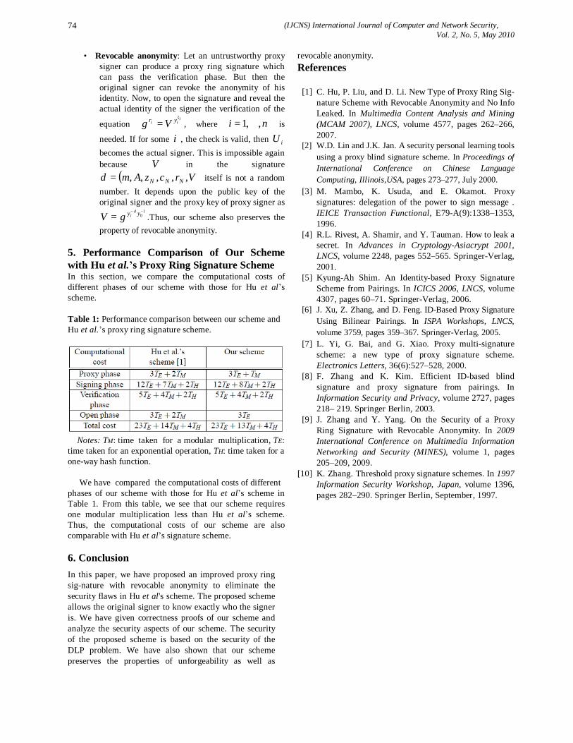
(IJCNS) International Journal of Computer and Network Security, Vol. 2, No. 5, May 2010
74
• Revocable anonymity: Let an untrustworthy proxy signer can produce a proxy ring signature which can pass the verification phase. But then the original signer can revoke the anonymity of his identity. Now, to open the signature and reveal the actual identity of the signer the verification of the
equation is
ii yr Vgˆ
= , where ni ,,1 ⋅⋅⋅= is
needed. If for some i , the check is valid, then iU
becomes the actual signer. This is impossible again because V in the signature
( )VrczAm NNN ,,,,,=δ itself is not a random number. It depends upon the public key of the original signer and the proxy key of proxy signer as
10−−
= yy digV .Thus, our scheme also preserves the
property of revocable anonymity. 5. Performance Comparison of Our Scheme with Hu et al.’s Proxy Ring Signature Scheme In this section, we compare the computational costs of different phases of our scheme with those for Hu et al’s scheme. Table 1: Performance comparison between our scheme and Hu et al.’s proxy ring signature scheme.
Notes: TM: time taken for a modular multiplication, TE: time taken for an exponential operation, TH: time taken for a one-way hash function. We have compared the computational costs of different phases of our scheme with those for Hu et al’s scheme in Table 1. From this table, we see that our scheme requires one modular multiplication less than Hu et al’s scheme. Thus, the computational costs of our scheme are also comparable with Hu et al’s signature scheme.
6. Conclusion In this paper, we have proposed an improved proxy ring sig-nature with revocable anonymity to eliminate the security flaws in Hu et al's scheme. The proposed scheme allows the original signer to know exactly who the signer is. We have given correctness proofs of our scheme and analyze the security aspects of our scheme. The security of the proposed scheme is based on the security of the DLP problem. We have also shown that our scheme preserves the properties of unforgeability as well as
revocable anonymity. References
[1] C. Hu, P. Liu, and D. Li. New Type of Proxy Ring Sig-nature Scheme with Revocable Anonymity and No Info Leaked. In Multimedia Content Analysis and Mining (MCAM 2007), LNCS, volume 4577, pages 262–266, 2007.
[2] W.D. Lin and J.K. Jan. A security personal learning tools using a proxy blind signature scheme. In Proceedings of International Conference on Chinese Language Computing, Illinois,USA, pages 273–277, July 2000.
[3] M. Mambo, K. Usuda, and E. Okamot. Proxy signatures: delegation of the power to sign message . IEICE Transaction Functional, E79-A(9):1338–1353, 1996.
[4] R.L. Rivest, A. Shamir, and Y. Tauman. How to leak a secret. In Advances in Cryptology-Asiacrypt 2001, LNCS, volume 2248, pages 552–565. Springer-Verlag, 2001.
[5] Kyung-Ah Shim. An Identity-based Proxy Signature Scheme from Pairings. In ICICS 2006, LNCS, volume 4307, pages 60–71. Springer-Verlag, 2006.
[6] J. Xu, Z. Zhang, and D. Feng. ID-Based Proxy Signature Using Bilinear Pairings. In ISPA Workshops, LNCS, volume 3759, pages 359–367. Springer-Verlag, 2005.
[7] L. Yi, G. Bai, and G. Xiao. Proxy multi-signature scheme: a new type of proxy signature scheme. Electronics Letters, 36(6):527–528, 2000.
[8] F. Zhang and K. Kim. Efficient ID-based blind signature and proxy signature from pairings. In Information Security and Privacy, volume 2727, pages 218– 219. Springer Berlin, 2003.
[9] J. Zhang and Y. Yang. On the Security of a Proxy Ring Signature with Revocable Anonymity. In 2009 International Conference on Multimedia Information Networking and Security (MINES), volume 1, pages 205–209, 2009.
[10] K. Zhang. Threshold proxy signature schemes. In 1997 Information Security Workshop, Japan, volume 1396, pages 282–290. Springer Berlin, September, 1997.
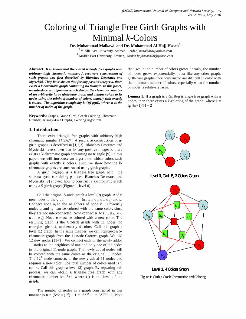
(IJCNS) International Journal of Computer and Network Security, Vol. 2, No. 5, May 2010
75
Figure 1: Girth g Graph Construction and Coloring
v1
v4
v5
v2
v3
Level 0, Girth 5, 3 Colors Graph
v1
v4
v5
v2
v3
Level 0, Girth 5, 3 Colors Graph
v1
v4
v5
v2
v3
Level 0, Girth 5, 3 Colors Graph
v1
v4
v5
v2
v3
Level 0, Girth 5, 3 Colors Graph
v1
v4
v5
v2
v3
Level 0, Girth 5, 3 Colors Graph
v1
v4
v5
v2
v3
Level 0, Girth 5, 3 Colors Graph
v1
v4
v5
v2
v3
Level 0, Girth 5, 3 Colors Graph
v1
v4
v5
v2
v3
u1
u2
u3u4
u5u
v1
v4
v5
v2
v3
u1
u2
u3u4
u5u
v1
v4
v5
v2
v3
u1
u2
u3
u4
u5u
Level 1, 4 Colors Graph
v1
v4
v5
v2
v3
u1
u2
u3u4
u5u
v1
v4
v5
v2
v3
u1
u2
u3u4
u5u
v1
v4
v5
v2
v3
u1
u2
u3
u4
u5u
Level 1, 4 Colors Graph
v1
v4
v5
v2
v3
u1
u2
u3
u4
u5u
Level 1, 4 Colors Graph
Coloring of Triangle Free Girth Graphs with Minimal k-Colors
Dr. Mohammad Malkawi1 and Dr. Mohammad Al-Hajj Hasan2
1Middle East University, Amman, Jordan, [email protected] 2 Middle East University, Amman, Jordan [email protected]
Abstract: It is known that there exist triangle free graphs with arbitrary high chromatic number. A recursive construction of such graphs was first described by Blanches Descrates and Mycielski. They have shown that for any positive integer k, there exists a k-chromatic graph containing no triangle. In this paper, we introduce an algorithm which detects the chromatic number of an arbitrarily large girth-base graph and assigns colors to its nodes using the minimal number of colors, namely with exactly k colors.. The algorithm complexity is O(Lg(n)), where n is the number of nodes of the graph. Keywords: Graphs, Graph Girth, Graph Coloring, Chromatic Number, Triangle-Free Graphs, Coloring Algorithm.
1. Introduction There exist triangle free graphs with arbitrary high
chromatic number [4,5,6,7]. A recursive construction of g-girth graphs is described in [1,2,3]. Blanches Descrates and Mycielski have shown that for any positive integer k, there exists a k-chromatic graph containing no triangle [9]. In this paper, we will introduce an algorithm, which colors such graphs with exactly k colors. First, we show how the k-chromatic graphs are constructed using girth graphs.
A girth g-graph is a triangle free graph with the shortest cycle containing g nodes. Blanches Descrates and Mycielski [9] showed how to construct a k-chromatic graph using a 5-girth graph (Figure 1, level 0).
Call the original 5-node graph a level (0) graph. Add 6 new nodes to the graph (u1, u 2, u 3, u 4, u 5) and u. Connect node ui to the neighbors of node vi . Obviously nodes ui and vi can be colored with the same color, since they are not interconnected. Now connect u to (u1, u 2, u 3, u 4, u 5). Node u must be colored with a new color. The resulting graph is the Grötzch graph with 11 nodes, no triangles, girth 4, and exactly 4 colors. Call this graph a level (1) graph. In the same manner, we can construct a 5-chromatic graph from the 11-node Grötzch graph. We add 12 new nodes (11+1). We connect each of the newly added 11 nodes to the neighbors of one and only one of the nodes in the original 11-node graph. The newly added nodes will be colored with the same colors as the original 11 nodes. The 12th node connects to the newly added 11 nodes and requires a new color. The total number of colors used is 5 colors. Call this graph a level (2) graph. By repeating this process, we can obtain a triangle free graph with any chromatic number k= 3+i, where (i) is the level of the graph.
The number of nodes in a graph constructed in this
manner is n = (5*2i)+( 2i) – 1 = 6*2i– 1 = 3*2k-2– 1. Note
that, while the number of colors grows linearly, the number of nodes grows exponentially. Just like any other graph, girth-base graphs once constructed are difficult to color with the minimum number of colors, especially when the number of nodes is relatively large.
Lemma 1: If a graph is a Girth-g triangle free graph with n nodes, then there exists a k-coloring of the graph, where k = lg [(n+1)/3] + 2
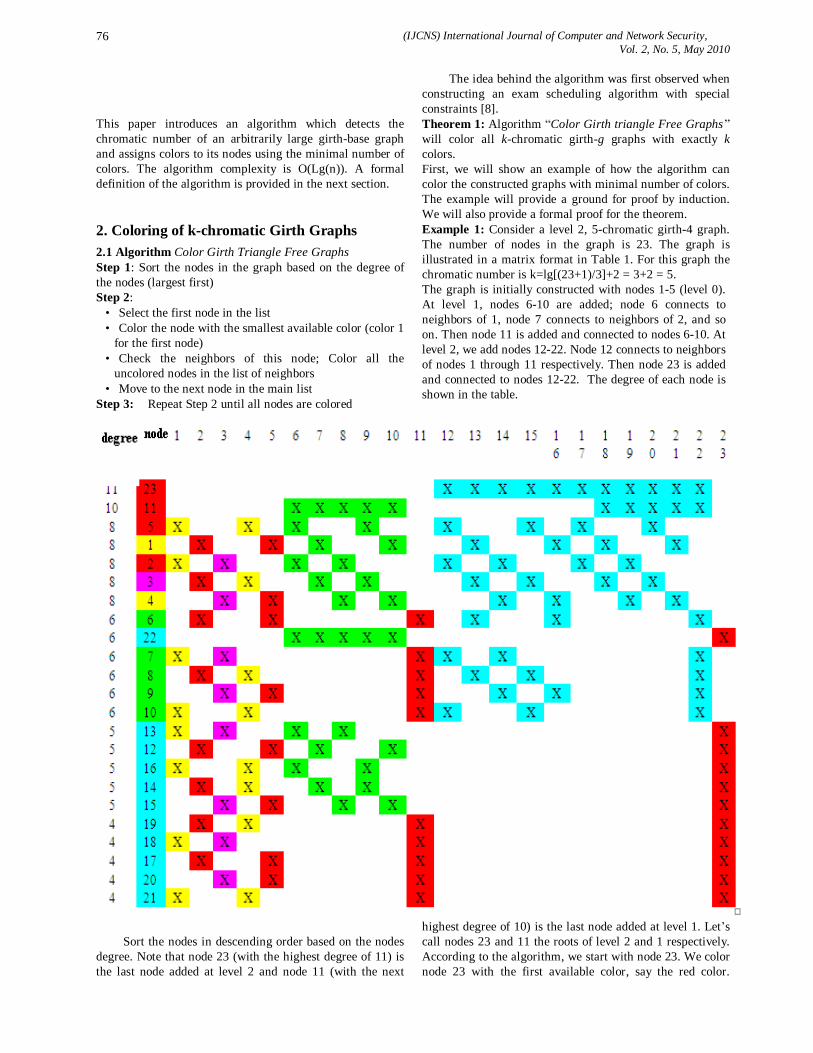
(IJCNS) International Journal of Computer and Network Security, Vol. 2, No. 5, May 2010
76
This paper introduces an algorithm which detects the chromatic number of an arbitrarily large girth-base graph and assigns colors to its nodes using the minimal number of colors. The algorithm complexity is O(Lg(n)). A formal definition of the algorithm is provided in the next section.
2. Coloring of k-chromatic Girth Graphs 2.1 Algorithm Color Girth Triangle Free Graphs Step 1: Sort the nodes in the graph based on the degree of the nodes (largest first) Step 2:
• Select the first node in the list • Color the node with the smallest available color (color 1
for the first node) • Check the neighbors of this node; Color all the
uncolored nodes in the list of neighbors • Move to the next node in the main list
Step 3: Repeat Step 2 until all nodes are colored
The idea behind the algorithm was first observed when constructing an exam scheduling algorithm with special constraints [8]. Theorem 1: Algorithm “Color Girth triangle Free Graphs” will color all k-chromatic girth-g graphs with exactly k colors. First, we will show an example of how the algorithm can color the constructed graphs with minimal number of colors. The example will provide a ground for proof by induction. We will also provide a formal proof for the theorem. Example 1: Consider a level 2, 5-chromatic girth-4 graph. The number of nodes in the graph is 23. The graph is illustrated in a matrix format in Table 1. For this graph the chromatic number is k=lg[(23+1)/3]+2 = 3+2 = 5. The graph is initially constructed with nodes 1-5 (level 0). At level 1, nodes 6-10 are added; node 6 connects to neighbors of 1, node 7 connects to neighbors of 2, and so on. Then node 11 is added and connected to nodes 6-10. At level 2, we add nodes 12-22. Node 12 connects to neighbors of nodes 1 through 11 respectively. Then node 23 is added and connected to nodes 12-22. The degree of each node is shown in the table.
Sort the nodes in descending order based on the nodes
degree. Note that node 23 (with the highest degree of 11) is the last node added at level 2 and node 11 (with the next
highest degree of 10) is the last node added at level 1. Let’s call nodes 23 and 11 the roots of level 2 and 1 respectively. According to the algorithm, we start with node 23. We color node 23 with the first available color, say the red color.
(IJCNS) International Journal of Computer and Network Security, Vol. 2, No. 5, May 2010
77
Node 23 has 11 neighbors. All the neighbors can be colored with the same color, since by definition they are not interconnected with each other. So we color nodes 12-22 with blue. The number of nodes colored at this step is (1+11) = 12. Actually this is equal to the number of nodes added at level 2, i.e., (N+1)/2.
Next we move down the list to the root node at level 1,
i.e., node 11 with degree 10. By definition, node 11 is not connected to node 23. Thus it may reuse the red color. Half of the neighbors of node 11 are also neighbors of node 23 since they were added at the second level, and thus they must have been colored at the previous step with the blue color (nodes 19-22). The other half (nodes 6-10) were added at level 1. Each of these nodes is connected to at least one of the nodes that have been colored at the previous step. A new color, say color green, is required to color nodes 6-10. Note that nodes 6-10 are not connected within each other, so they all can use the same color. At the end of this step, all nodes added at level one (5+1) are colored, and only one new color is added.
The next node in the list is node 5. Note that at this stage, we have arrived at the original 5 nodes cycle (1 through 5). All of these nodes have the same degree. So we can start with any of them and get the same result. Node 5 has 8 neighbors. 6 out of 8 nodes have already been colored with colors green and blue. Node 5 can take the color red. Note that color red is only used by the root nodes (11 and 23) at levels 1 and 2. These nodes do not connect to any of the inner most 5-nodes cycle. The neighbors of 5 (nodes 1 and 4) require a new color, say the yellow color. The total number of nodes colored at this stage is (2+1). It is worth noting that the inner 5-node cycle requires at most 3 colors. One of the already used colors can certainly be reused. This is the color given to the root nodes added at each of the subsequent levels of the graph construction. So, when the algorithm reaches the last 5 nodes in the graph, only 2 new colors will be required. The next node in the list is node 1. Node 1 has already been colored with the yellow color. All the neighbors of node 1 have been colored except for node 2, which can take the color red. The next node in the list is node 2. Node 2 has already been colored. All of its neighbors are colored except for node 3. Node 3 requires a new color, say the color pink.
At this stage all the nodes of the graph have been colored with five colors, and the algorithm terminates. The termination criterion of the algorithm is simple. The algorithm maintains a list of all the nodes that have not been colored. Every time a node is colored, the node will be removed from the list. The algorithm terminates when the list becomes empty. We observe the followings from the process of coloring the graph. 1. The number of nodes and colors covered at each stage
are as follows: a. First stage: 12 nodes = ((23+1)/2). Number of colors
used is 2 b. 2nd stage: 6 nodes = ((23+1)/4). Number of colors is
1
c. 3rd stage: 3 nodes (23+1/8). Number of colors is 1 d. 4th and 5th stages: 2 nodes. Number of colors is 1
2. The total number of steps required to color the graph is 5 = 23Lg
2.2 Proof:
We now present a formal proof of the theorem. By construction, a girth graph consists of two major parts; the foundation, which is the 5-node cycle, and a multi-level structure of nodes. Each level adds twice the number of nodes to the previous level plus one root. The root at each level is connected only to the newly added nodes, and is isolated from all the nodes added at the previous level(s). The largest degree node is the root of the last level in the graph. The degree of this node is d=(N-1)/2. The next largest degree node is the root of the next level down, with degree = d-1, and so on.
The algorithm sorts the nodes of the graph in a descending order based on the degree of nodes. By definition, the largest degree node is the root of the last (highest) level.
Assume that we construct a girth graph with (i) levels. For (i=0), the graph has 5 nodes. For (i=1), the graph has 11 nodes. For (i=5), the graph has 191 nodes. At the (ith) level, the number of nodes is N=(5*2i)+( 2i)-1. The node with the largest degree is the last node added to the graph, i.e., the root at level (i) and is connected to (N-1)/2-1 nodes; so the degree at level (i) di = (3*2i-1). The next largest degree node is the root node added at the previous level (i-1). This node is connected to nodes at the current level (i-1) and nodes at the upper level (i). The number of nodes connected at the current level (i-1) = (3*2i-1-1). The number of nodes connected to the root at the upper level (i) is = (3*2i-1-1). So the degree at level (i-1), di-1 =2*(3*2i-1-1) = 3*2i-2. The next largest degree node is the root at level (i-2). The root is connected to (3*2i-2-1) nodes at level (i-2). It is connected to same number of nodes at level (i-1). It is also connected to 2*(3*2i-2-1) at level (i). So the degree at level (i-2) di-2 = (3*2i-2-1) + (3*2i-2-1) + 2*(3*2i-2-1) = (3*2i-2-1)*22. In general, the degree of a root node at level (i-k), where k = 0,1, 2, … (i-2) is given by di-k= (3*2i-k-1)* 2k.
For example, let (i=5). The total number of nodes in the graph is (6*25-1) = 191. d5= (3*25-1) = 95; d4= 2*(3*24-1) = 94; d3= 22*(3*23-1) = 92; d2= 23*(3*22-1) = 88.
The algorithm sorts the nodes based on node degrees in a descending order. Thus, the algorithm will color the nodes starting with the roots at each level.
At level (i), the algorithm will color the root node and all its adjacent nodes. Since the adjacent nodes are not interconnected, they can assume the same color. The root will have a different color. So step one, will consume two colors. The next step will take care of the nodes at the next lower level. Since the root at this level is not connected to the root at the upper level, it can assume the color of the root at the upper level; so no new color is consumed. The neighbors of the root at this level are split in two sets. One set belongs to the upper level, so this set has already been colored. The second set is not inter-connected, so the nodes of this set can all be colored with the same color. A new color will be consumed. Similarly, at the next level, the root

(IJCNS) International Journal of Computer and Network Security, Vol. 2, No. 5, May 2010
78
can assume the same colors of the previous roots, since they are not interconnected. The neighbors of this node are split in 3 sets. Two sets belong to the upper 2 levels and one set belongs to the current level. The nodes, which belong to the upper 2 levels, have been colored at the previous steps. The nodes in the current level are not interconnected, so they can assume one color. Continuing in this manner, the algorithm will consume one color at each level until it reaches the lowest 5 nodes in the graph, where it will consume 2 new colors.
Thus, the algorithm detects the structure of the graph and colors the nodes with the minimal number of
colors ∑+
+1
12i
. The algorithm also uses minimum number
of steps because it colors the roots and their neighbors first.
3. Conclusions This paper presents a coloring algorithm which colors
a girth-g, triangle free graphs with arbitrarily large k-chromatic number. The algorithm detects the structure of a girth-g graph and colors the graph with exactly k colors. The algorithm terminates in O(Lg(n)) steps.
References
[1] Bollobas,B., Sauer,N.: ”Uniquely Colorable Graphs with Large Girth,” Canad. J. Math. 28 (1976), no. 6, 1340-1344.
[2] Emden-Weinert,T., Hougardy,S., Kreuter,B.: ”Uniquely Colorable Graphs and the Hardness of Coloring Graphs of Large Girth,” Com-bin. Probab. Comput. 7 (1998), no. 4, 375-386.
[3] Erdos,P.: ”Graph Theory and Probability,” Canad. J. Math 11 (1959), 34-38.
[4] Muller,V.: ”On Colorings of Graphs Without Short Cycles,” Discrete Mathematics 26 (1979), 165-176.
[5] Nesetril,J., Zhu,X.: ”Construction of Sparse Graphs with Prescribed Circular Colorings,” Discrete Mathematics 233 (2001), 277-291.
[6] Steffen,E., Zhu,X.: ”Star Chromatic Numbers of Graphs,” Combinatoria 16 (1996), no. 3, 439-448.
[7] Zhu,X.: ”Uniquely H-colorable Graphs with Large Girth”, J. Graph Theory 23 (1996), no. 1, 33-41.
[8] Mohammad Malkawi, Mohammad Al-Haj Hassan, and Osama Al-Haj Hassan, “A New Exam Scheduling Algorithm Using Graph Coloring”, The International Arab Journal of Information Technology, Vol. 5, No. 1, 2008; pp. 80-86.
[9] Soifer, Alexander “Mathematics of Coloring and the Colorful Life of its Creators”, Springer; pp, 83-86; ISBN: 978-0-387-74640-1
Authors Profile
Dr. Mohammad Malkawi received his Ph.D. degree in computer engineering from the University of Illinois at Urbana-Champaign in 1986. He received his BS and MS in computer engineering in 1980 and 1983. He was a member of the High Productivity Computing Systems team at
SUN Microsystems, and the high availability platform team at Motorola. Currently, he is associate professor at Middle East University in Jordan.
Mohammad M Al-Haj Hassan obtained his B.Sc. and Master degrees from The University of Jordan in 1973 and 1977 respectively, and his Ph.D. degree in Computer Science from Clarkson University at NY / USA. His main field of Specialization is Computer Algorithms with specific concentration on Graph Algorithms & Their Applications. Other fields of research are: Machine Learning, Parallel Computations and Algorithms,
Distance Learning and Web-Based Courses Design. Professor M. Al-Haj Hassan was the Dean of several Faculties in several universities. He is a member in the Editorial Board and/or referee of several journals. He has been the Secretary General of The International Arab Conference on Information Technology (ACIT) for 4 years. Currently, he is a professor of Computer Science and the Vice President at Middle East University in Jordan.

(IJCNS) International Journal of Computer and Network Security, Vol. 2, No. 5, May 2010
79
An Efficient Solution for Privacy Preserving Association Rule Mining
Chirag N. Modi1, Udai Pratap Rao1 and Dhiren R. Patel2
1Department of Computer Engineering, Sardar Vallabhbhai National Institute of Technology,
Ichchhanath, Surat, India-395 007 [email protected]
2Department of Computer Science & Engineering, Indian Institute of Technology Gandinagar, Ahmedabad, Gujarat, India-382 424
Abstract: The recent advances of data mining techniques played an important role in many areas for various applications. However the misuse of these techniques may disclose the private or sensitive information which database owners do not want reveal to others. To preserve privacy for sensitive association rules in statistical databases, many approaches have been found. In this paper, we propose two heuristic blocking based algorithms named ISARC (Increase Support of common Antecedent of Rule Clusters) and DSCRC (Decrease Support of common Consequent of Rule Clusters) to preserve privacy for sensitive association rules. Proposed algorithms cluster the sensitive rules based on some criteria and hide them in fewer selected transactions by using unknowns (“?”). They preserve certain privacy for sensitive rules in database, while maintaining knowledge discovery. An example illustrating proposed algorithms is given. We also discuss the performance results of both the algorithms.
Keywords: Data Mining, Association Rule Hiding, Knowledge Hiding, Clustering, Sensitivity, Database Security and Privacy.
1. Introduction Recently privacy preserving data mining (PPDM) become a hot directive to prevent disclosure of sensitive knowledge or rules by data mining techniques. M.Attallah et al. [1] was the first to present disclosure limitation of sensitive knowledge by data mining algorithms and proposed heuristic algorithms to prevent disclosure of sensitive knowledge. The authors in [2] presented some suggestions for defining and measuring privacy preservation and showed how these relate to both privacy policy and practice in wider community and to techniques in privacy preserving data mining. Oliveria and Saygin et al. [4] presented taxonomy of attacks against sensitive knowledge. Clifton et al. [7] was the first to show the importance of association rule hiding and also discussed security and privacy implication of data mining.
1.1 Motivation Consider, as a tea reseller we are purchasing tea at low price from two companies, Tata Tea Ltd. and Lipton Tea Ltd., while granting them to access our customer database. Now,
suppose the Lipton Tea supplier misuse the database and mines association rules related to the Tata Tea, saying that most of the customers who buy bread also buy Tata tea. Lipton tea supplier now runs a coupon scheme that offers some discount on bread with purchase of Lipton Tea. So, the amount of sales on Tata Tea is down rapidly and Tata Tea supplier cannot offer tea at low price to us as before and Lipton monopolizes the tea market and is not offering tea at low price to us as before. As a result, we may start losing business to our competitors. So, releasing database with sensitive knowledge is bad for us. This scenario leads to the research of sensitive knowledge (or rule) hiding in database.
The knowledge privacy problem, in context of association rule mining which is proved NP hard in [1]. There are several heuristic techniques have been found to solve above problem. M.Attallah et al. [1] were the first to propose heuristic algorithms which decrease significance of the rules for hiding the sensitive rules in databases. Verykios et al. [5] proposed five algorithms which reduce the support or confidence of sensitive rules by removing or inserting some items in selected transactions. These algorithms hide only one sensitive rule or sensitive item at a time and provide certain privacy. Y-H Wu et al. [10] proposed a method to reduce the side effects produced by sanitization, which formulates set of constraints related to the possible side effects and allows item modification based on more significant constraint. K.Duraiswamy et al. [9] proposed an efficient clustering based approach that clusters the sensitive rules based on common item in R.H.S. of the sensitive rules and hides the R.H.S. items in each cluster by reducing support of it.
Y.Saygin et al. [8][11] were the first proposed blocking approach to increase or decrease the support of item by placing unknowns (“?”) in place of 1’s or 0’s .So, It is difficult for an adversary to know the value behind unknowns (“?”). The safety margin is also used to show how much below the minimum threshold new significance of a rule should. This approach is effective and provides certain privacy. Wang and Jafari [6] proposed more efficient approaches than other approaches as in [8][11]. They require less number of database scans and prune more

(IJCNS) International Journal of Computer and Network Security, Vol. 2, No. 5, May 2010
80
number of rules, while hiding many rules at a time. But they produce undesirable side effects.
In this paper, we propose two heuristic blocking based algorithms named ISARC (Increase Support of common Antecedent of Rule Clusters) and DSCRC (Decrease Support of common Consequent of Rule Clusters) to preserve privacy for sensitive association rules in database. To hide sensitive rules, proposed algorithms replace the 1’s or 0’s by unknowns (“?”) in fewer selected transactions for decreasing their confidence. So, it is difficult for an adversary to know the value behind unknowns (“?”). To decrease the confidence of specified rules, first algorithm increases the support of rule antecedent, while another decreases the support of rule consequent. They can hide many rules at a time in rule clusters. So, they are more efficient than other heuristic approaches. Moreover they maintain data quality in database.
The rest of this paper is organized as follows: In section 2, we discuss some related background and concepts, while a detailed description of proposed algorithms (ISARC and DSCRC) is given in section 3. An example illustrating ISARC and DSCRC is given in section 4. In section 5 we discuss and analyze the performance results of both the proposed algorithm. Finally in section 6, we conclude proposed algorithms by defining some future trends.
2. Theoretical Background and Preliminaries
The standard definition of association rule is given in [5], which is as follows: Let I=i1,…,imbe a set of items. Database D=T1,….,Tnis a set of transactions, where Ti⊆I(1≤i≤m). Each transaction T is an itemset such that T⊆I. We say that a transaction T supports X, a set of items in I, if X⊆I. The association rule is an implication formula like X⇒Y, where X⊂I, Y⊂I and X∩Y=∅. The itemset X∪Y called generating itemset which lead to the generation of an association rule which is consists of two parts: left hand side (L.H.S.) item (X) called rule antecedent and right hand side (R.H.S) item (Y) called rule consequent. The rule with support s and confidence c is called, if |X∪Y|/|D| ≥ s and |X∪Y|/|X| ≥ c. Because of interestingness, we consider user specified thresholds for support and confidence, MST (minimum support threshold) and MCT (minimum confidence threshold). A detailed overview of association rule mining algorithms are presented in [3].
2.1 Problem Description Let given dataset D, a set of association rules R over D is given and also Rh⊆R, Rh is specified as sensitive rules set. Now, the problem is to find sanitized database D’ such that there exist only a set of rules R-Rh, can be mined. It should achieve one of the following goals: (1) All the sensitive association rules must be hidden in sanitized database. (2) All the rules that are not specified as sensitive can be mined from sanitized database. (3) No new rule that was not previously found in original database can be mined from
sanitized database. First goal considers privacy issue. Second goal is related to the usefulness of sanitized dataset. Third goal is related to the side effect of the sanitization process.
2.2 Basic Concepts
2.2.1 Rule Hiding by Reducing Confidence To hide an association rule like X ⇒Y, we decrease its confidence (|X∪Y|/|X|) to be smaller than pre-specified minimum confidence threshold (MCT). To decrease the confidence of a rule, two strategies as in [5] can be considered. The first one is to increase the support of rule antecedent (X), but not support of generating itemset (X∪Y). The second one is to decrease the support of generating itemset (X∪Y). To decrease support of generating itemset, we decrease the support of rule consequent Y only in transactions containing both X and Y. So, it can reduce the rule confidence faster than reducing the support of X.
2.2.2 Increasing or Decreasing Support of item by using Unknowns
Instead of distorting transactions, we increase or decrease support of one item at a time in a selected transaction by replacing from 0 to unknowns (“?”) or 1 to unknowns (“?”) respectively. A detailed overview of unknown technique to decrease or increase support of item is given in [8].
2.2.3 Clustering We cluster the sensitive rules based on common antecedent or common consequent to hide many rules at a time by replacing fewer 1’s or 0’s to unknowns (“?”) in selected transactions.
2.2.4 Sensitivity We use sensitive characteristics of sensitive rules to select transactions for modification. A detailed overview of sensitivities is given in [13]. Following sensitivities are used in our proposed algorithms: (1) Item Sensitivity: is the frequency of data item exists in the number of the sensitive association rules containing sensitive item. It is used to measure rule sensitivity. (2) Rule Sensitivity: is the sum of the sensitivities of all items containing that association rule. (3) Cluster Sensitivity: is the sum of the sensitivities of all association rules in cluster. Cluster sensitivity defines the rule cluster which is most affecting to the privacy. (4) Sensitive Transaction: is the transaction in given database which contains sensitive item. (5) Transaction sensitivity: is the sum of sensitivities of sensitive items contained in the transaction.
3. ISARC and DSCRC - Proposed Privacy Preserving Association Rule Mining Algorithms
3.1 Proposed Framework The proposed common framework for ISARC and DSCRC is shown in Fig. 1. As shown in Fig. 1, First both the
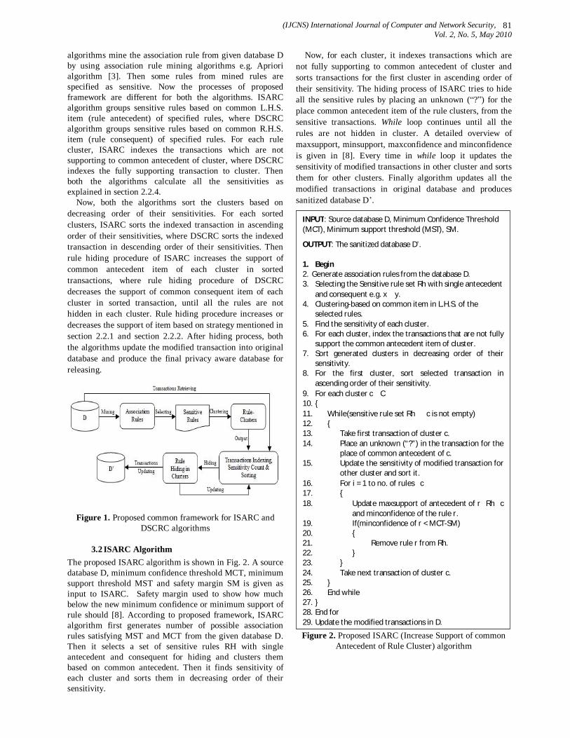
(IJCNS) International Journal of Computer and Network Security, Vol. 2, No. 5, May 2010
81
algorithms mine the association rule from given database D by using association rule mining algorithms e.g. Apriori algorithm [3]. Then some rules from mined rules are specified as sensitive. Now the processes of proposed framework are different for both the algorithms. ISARC algorithm groups sensitive rules based on common L.H.S. item (rule antecedent) of specified rules, where DSCRC algorithm groups sensitive rules based on common R.H.S. item (rule consequent) of specified rules. For each rule cluster, ISARC indexes the transactions which are not supporting to common antecedent of cluster, where DSCRC indexes the fully supporting transaction to cluster. Then both the algorithms calculate all the sensitivities as explained in section 2.2.4.
Now, both the algorithms sort the clusters based on decreasing order of their sensitivities. For each sorted clusters, ISARC sorts the indexed transaction in ascending order of their sensitivities, where DSCRC sorts the indexed transaction in descending order of their sensitivities. Then rule hiding procedure of ISARC increases the support of common antecedent item of each cluster in sorted transactions, where rule hiding procedure of DSCRC decreases the support of common consequent item of each cluster in sorted transaction, until all the rules are not hidden in each cluster. Rule hiding procedure increases or decreases the support of item based on strategy mentioned in section 2.2.1 and section 2.2.2. After hiding process, both the algorithms update the modified transaction into original database and produce the final privacy aware database for releasing.
Figure 1. Proposed common framework for ISARC and DSCRC algorithms
3.2 ISARC Algorithm The proposed ISARC algorithm is shown in Fig. 2. A source database D, minimum confidence threshold MCT, minimum support threshold MST and safety margin SM is given as input to ISARC. Safety margin used to show how much below the new minimum confidence or minimum support of rule should [8]. According to proposed framework, ISARC algorithm first generates number of possible association rules satisfying MST and MCT from the given database D. Then it selects a set of sensitive rules RH with single antecedent and consequent for hiding and clusters them based on common antecedent. Then it finds sensitivity of each cluster and sorts them in decreasing order of their sensitivity.
Now, for each cluster, it indexes transactions which are not fully supporting to common antecedent of cluster and sorts transactions for the first cluster in ascending order of their sensitivity. The hiding process of ISARC tries to hide all the sensitive rules by placing an unknown (“?”) for the place common antecedent item of the rule clusters, from the sensitive transactions. While loop continues until all the rules are not hidden in cluster. A detailed overview of maxsupport, minsupport, maxconfidence and minconfidence is given in [8]. Every time in while loop it updates the sensitivity of modified transactions in other cluster and sorts them for other clusters. Finally algorithm updates all the modified transactions in original database and produces sanitized database D’.
Figure 2. Proposed ISARC (Increase Support of common
Antecedent of Rule Cluster) algorithm
INPUT: Source database D, Minimum Confidence Threshold (MCT), Minimum support threshold (MST), SM.
OUTPUT: The sanitized database D’. 1. Begin 2. Generate association rules from the database D. 3. Selecting the Sensitive rule set Rh with single antecedent
and consequent e.g. x⇒y. 4. Clustering-based on common item in L.H.S. of the
selected rules. 5. Find the sensitivity of each cluster. 6. For each cluster, index the transactions that are not fully
support the common antecedent item of cluster. 7. Sort generated clusters in decreasing order of their
sensitivity. 8. For the first cluster, sort selected transaction in
ascending order of their sensitivity. 9. For each cluster c∈ C 10. 11. While(sensitive rule set Rh ∈ c is not empty) 12. 13. Take first transaction of cluster c. 14. Place an unknown (“?”) in the transaction for the
place of common antecedent of c. 15. Update the sensitivity of modified transaction for
other cluster and sort it. 16. For i = 1 to no. of rules∈c 17. 18. Update maxsupport of antecedent of r∈Rh∈c
and minconfidence of the rule r. 19. If(minconfidence of r < MCT-SM) 20. 21. Remove rule r from Rh. 22. 23. 24. Take next transaction of cluster c. 25. 26. End while 27. 28. End for 29. Update the modified transactions in D.

(IJCNS) International Journal of Computer and Network Security, Vol. 2, No. 5, May 2010
82
3.3 DSCRC Algorithm The proposed DSCRC algorithm is shown in Fig. 3. It clusters the sensitive rules based on common R.H.S. item of rules and sorts sensitive transaction in decreasing order of their sensitivities.
The hiding process of DSCRC tries to hide all the sensitive rules by placing an unknown (“?”) for the place common consequent of the rule clusters, from the sensitive transactions. While loop continues until all the rules are not hidden in cluster c. Every time in while loop it updates the sensitivity of modified transaction in other cluster and sorts them for other clusters. Finally algorithm updates all the modified transactions in original database and produces sanitized database D’, in which most of the sensitive rules are hidden.
Figure 3. Proposed DSCRC (Decrease Support of common Consequent of Rule Cluster) algorithm
Both the proposed ISARC and DSCRC algorithms hide many rules in an iteration of hiding process and modify fewer transactions in database. But DSCRC hides rules faster than ISARC, because it reduces the confidence of sensitive rule faster than ISARC. The safety margin is also used in both the algorithms to provide better privacy.
4. Example A sample transaction database D taken from [8] is shown in Table 1. TID shows unique transaction number. Binary valued item shows whether an item is present or absent in that transaction. Suppose MST, MCT and SM are selected 50%, 70% and 0 respectively. Table 2 shows frequent itemsets satisfying MST, generated from sample database D. In following, the possible number of association rules satisfying MST and MCT, generated by Apriori algorithm [2] are given: 0⇒1, 1⇒0, 0⇒3, 3⇒0. Suppose the rules 0⇒1 and 0⇒3 are specified as sensitive and should be hidden in sanitized database. There are one different L.H.S. item in selected rules, named “0” and two different R.H.S. items in selected rules, named “1” and “3”. As shown in Table 3(a), ISARC algorithm generates one cluster based on common L.H.S. item of the selected rules, where Table 3(b) shows rule clusters based on common R.H.S. item of the selected rules, generated by DSCRC algorithm.
Table 1: Sample database D
TID Items
Items (Binary Form)
0 0 1 3 1101
1 1 0100
2 0 2 3 1011
3 0 1 1100
4 0 1 3 1101
Table 2: Frequent itemsets in sample database D
Frequent Itemsets with Support(%)
0:80, 1:80, 3:60, 01:60, 03:60 For ISARC algorithm, cluster 1 includes sensitive rules
namely 0⇒1 and 0⇒3. For cluster 1 sensitivities of items 0, 1, and 3 have 2, 1 and 1 respectively. Total sensitivity for cluster-1 is 6. For DSCRC algorithm, cluster 1 includes sensitive rule namely 0⇒1, where cluster 2 includes 0⇒3. For cluster 1 sensitivities of items 0 and 1 have 1 and 1 respectively, where sensitivities for items 0 and 3 in cluster 2 have 1and 1 respectively. Total sensitivity for cluster-1 and cluster-2 is 2 and 2 respectively.
INPUT: Source database D, Minimum Confidence Threshold (MCT), Minimum support threshold (MST).
OUTPUT: The sanitized database D’. 1. Begin 2. Generate association rules from the database D.
Selecting the Sensitive rule set Rh with single antecedent and consequent e.g. x⇒y.
4. Clustering based on common item in R.H.S. of the selected rules.
5. Find the sensitivity of each cluster. For each cluster, index the transactions that are fully
support the rules of cluster. 7. Sort generated clusters in decreasing order of their
sensitivity. 8. For the first cluster, sort selected transaction in
decreasing order of their sensitivity 9. For each cluster c∈ C 10. 11. While(sensitive rule set Rh ∈ c is not empty) 12. 13. Take first transaction of cluster c. 14. Place an unknown (“?”) in the transaction for the
place of common consequent of c. 15. Update the sensitivity of modified transaction for
other cluster and sort it. 16. For i = 1 to no. of rules∈c 17. 18. Update minsupport and minconfidence of the
rule r∈Rh∈c. 19. If(minconfidence of r < MCT-SM or
minsupport of r < MST-SM) 20. 21. Remove rule r from Rh. 22. 23. 24. Take next transaction of cluster c. 25. 26. End while 27. 28. End for 29. Update the modified transactions in D.
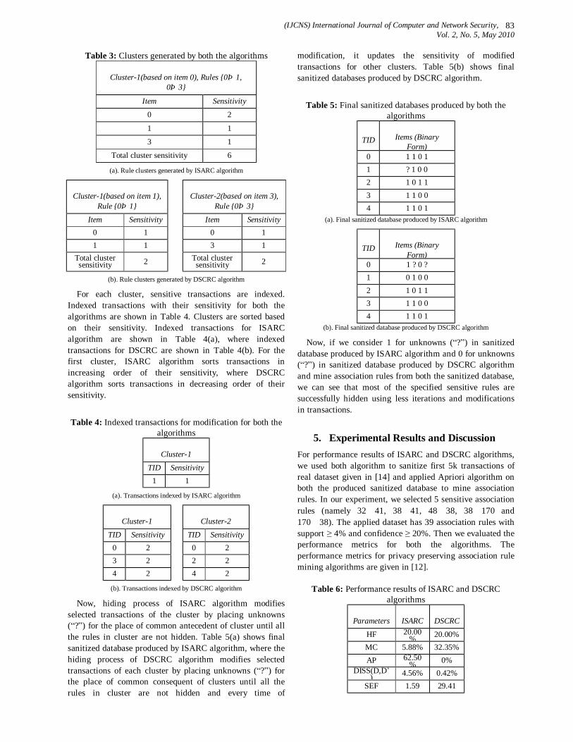
(IJCNS) International Journal of Computer and Network Security, Vol. 2, No. 5, May 2010
83
Table 3: Clusters generated by both the algorithms
Cluster-1(based on item 0), Rules 0⇒1, 0⇒3
Item Sensitivity
0 2
1 1
3 1
Total cluster sensitivity 6
(a). Rule clusters generated by ISARC algorithm
Cluster-1(based on item 1), Rule 0⇒1
Cluster-2(based on item 3), Rule 0⇒3
Item Sensitivity Item Sensitivity 0 1 0 1 1 1 3 1
Total cluster sensitivity 2
Total cluster sensitivity 2
(b). Rule clusters generated by DSCRC algorithm
For each cluster, sensitive transactions are indexed. Indexed transactions with their sensitivity for both the algorithms are shown in Table 4. Clusters are sorted based on their sensitivity. Indexed transactions for ISARC algorithm are shown in Table 4(a), where indexed transactions for DSCRC are shown in Table 4(b). For the first cluster, ISARC algorithm sorts transactions in increasing order of their sensitivity, where DSCRC algorithm sorts transactions in decreasing order of their sensitivity.
Table 4: Indexed transactions for modification for both the algorithms
Cluster-1
TID Sensitivity 1 1
(a). Transactions indexed by ISARC algorithm
Cluster-1 Cluster-2
TID Sensitivity TID Sensitivity 0 2 0 2 3 2 2 2 4 2 4 2
(b). Transactions indexed by DSCRC algorithm
Now, hiding process of ISARC algorithm modifies selected transactions of the cluster by placing unknowns (“?”) for the place of common antecedent of cluster until all the rules in cluster are not hidden. Table 5(a) shows final sanitized database produced by ISARC algorithm, where the hiding process of DSCRC algorithm modifies selected transactions of each cluster by placing unknowns (“?”) for the place of common consequent of clusters until all the rules in cluster are not hidden and every time of
modification, it updates the sensitivity of modified transactions for other clusters. Table 5(b) shows final sanitized databases produced by DSCRC algorithm.
Table 5: Final sanitized databases produced by both the algorithms
TID Items (Binary Form)
0 1 1 0 1 1 ? 1 0 0 2 1 0 1 1 3 1 1 0 0 4 1 1 0 1
(a). Final sanitized database produced by ISARC algorithm
TID Items (Binary Form)
0 1 ? 0 ? 1 0 1 0 0 2 1 0 1 1 3 1 1 0 0 4 1 1 0 1
(b). Final sanitized database produced by DSCRC algorithm
Now, if we consider 1 for unknowns (“?”) in sanitized database produced by ISARC algorithm and 0 for unknowns (“?”) in sanitized database produced by DSCRC algorithm and mine association rules from both the sanitized database, we can see that most of the specified sensitive rules are successfully hidden using less iterations and modifications in transactions.
5. Experimental Results and Discussion For performance results of ISARC and DSCRC algorithms, we used both algorithm to sanitize first 5k transactions of real dataset given in [14] and applied Apriori algorithm on both the produced sanitized database to mine association rules. In our experiment, we selected 5 sensitive association rules (namely 32⇒41, 38⇒41, 48⇒38, 38⇒170 and 170⇒38). The applied dataset has 39 association rules with support ≥ 4% and confidence ≥ 20%. Then we evaluated the performance metrics for both the algorithms. The performance metrics for privacy preserving association rule mining algorithms are given in [12].
Table 6: Performance results of ISARC and DSCRC algorithms
Parameters ISARC DSCRC
HF 20.00% 20.00%
MC 5.88% 32.35% AP 62.50
% 0% DISS(D,D’
) 4.56% 0.42% SEF 1.59 29.41

(IJCNS) International Journal of Computer and Network Security, Vol. 2, No. 5, May 2010
84
As shown in Table 6, performance results of ISARC and DSRRC are better in terms of hiding failure (HF), misses cost (MC), artifactual patterns (AP), dissimilarity (DISS), and side effect factor (SEF). They provide certain privacy and knowledge discovery. Here we selected 0.1% safety margin. If we select higher safety margin, both the algorithms provide more privacy to sensitive rules. Performance results of both the algorithms depend on database to modify and specified sensitive rules.
We can see that both the proposed algorithms hide many sensitive rules successfully, while maintaining knowledge discovery in terms of data quality By analyzing performance results,. The number of modifications in database is very less because of clustering and use of sensitivities. Efficiency is improved by clustering which helps to hide many rules at a time by modifying less sensitive transactions.
Suppose an adversary is more intelligent and he/she knows that the original database is modified by some safety margin and thresholds. If he/she mines association rules satisfying support and confidence below the MST-SM and MCT-SM respectively. Then he/she can derive sensitive rules from the sanitized database. Therefore, if random safety margin for each rule or each rule cluster is used in sanitization process, it can provide more privacy to sensitive rules.
6. Conclusion and Future Scope In this paper, we proposed two algorithms named ISARC and DSCRC to hide sensitive rules in database for privacy issue. Both algorithms provide certain privacy to sensitive rules by using unknowns and maintain data quality for knowledge discovery. Through an example we have demonstrated proposed algorithms and analyzed performance results. Both algorithms can hide rules which have single antecedent or consequent and they are more efficient than other heuristic approaches.
Proposed algorithms viz; ISARC and DSCRC can be modified to hide sensitive rules which have different number of L.H.S. items or R.H.S. items. In future, a parallelization can be also applied to improve efficiency of proposed algorithms.
References [1] M. Atallah, E. Bertino, A.K. Elmagarmid, M. Ibrahim,
V.S. Verykios. “Disclosure Limitation of Sensitive Rules”. In Proceedings of the 1999 IEEE Knowledge and Data Engineering Exchange Workshop (KDEX 1999), pp. 45-52, 1999.
[2] C. Clifton, M. Kantarcioglu, J. Vaidya. “Defining Privacy for Data Mining”. In Proceedings US Nat'l Science Foundation Workshop on Next Generation Data Mining, pp. 126-133, 2002.
[3] J. Han, M. Kamber. Data Mining: Concepts and Techniques, Morgan Kaufmann Publishers, San Francisco, pp. 227–245, 2001.
[4] S.R.M. Oliveira, O.R. Zaïane, Y. Saygın. “Secure Association Rule Sharing”. In Proceedings of the 8th Pacific-Asia Conference on PAKDD2004, Sydney, Australia, pp. 74–85, 2004.
[5] V.S. Verykios, A.K. Elmagarmid, E. Bertino, Y. Saygin, E. Dasseni. “Association Rule Hiding”. IEEE Transactions on Knowledge and Data Engineering, Vol. 16, no. 4, pp. 434–447, 2004.
[6] S.L. Wang, A. Jafari. “Using Unknowns for Hiding Sensitive Predictive Association Rules”. In Proceedings IEEE International Conference on Information Reuse and Integration (IRI 2005), pp. 223–228, 2005.
[7] C. Clifton, D. Marks. “Security and Privacy Implications of Data Mining”. In Proceedings ACM SIGMOD International Conference on Management of Data (SIGMOD’96), pp. 15–19, 1996.
[8] Y. Saygin, V.S. Verykios, C. Clifton. “Using Unknowns to Prevent Discovery of Association Rules”. ACM SIGMOD, Vol. 30, no. 4, pp. 45–54, 2001.
[9] K. Duraiswamy, D. Manjula. “Advanced Approach in Sensitive Rule Hiding”. Modern Applied Science, Vol. 3, no. 2, 2009.
[10] Y.H. Wu, C.M. Chiang, A.L.P. Chen. “Hiding Sensitive Association Rules with Limited Side Effects”. IEEE Transactions on Knowledge and Data Engineering, Vol. 19, no. 1, pp. 29–42, 2007.
[11] Y. Saygin, V.S. Verykios, A.K. Elmagarmid. “Privacy Preserving Association Rule Mining”. In Proceedings International Workshop on Research Issues in Data Engineering (RIDE 2002), pp.151–163, 2002.
[12] C.C. Aggarwal, P.S. Yu. Privacy-Preserving Data Mining: Models and Algorithms, Springer, Heidelberg, pp. 267–286, 2008.
[13] S. Wu, H. Wang. “Research On The Privacy Preserving Algorithm Of Association Rule Mining In Centralized Database”. International Symposiums on Information Processing (ISIP), pp. 131 – 134, 2008.
[14] T. Brijis, G. Swinnen, K.Vanhoof and G. Wets, “The use of association rules for product assortment decisions: a case study,” In Proceedings of the Fifth International Conference on Knowledge Discovery and Data Mining, San Diego (USA), pp. 254-260, 1999.
Authors Profile
Chirag N. Modi was born in Patan, Gujarat, India, on 3rd Feb 1987. He received his B.E. degree in Computer Engineering from S.P. University Anand (Gujarat)-India in 2008. He is Pursuing M.Tech degree in Computer Engineering at S. V. National Institute of Technology Surat (Gujarat)-India. His research interests include Data Mining and
Database security.

(IJCNS) International Journal of Computer and Network Security, Vol. 2, No. 5, May 2010
85
Udai Pratap Rao received the B.E. degree in Computer Science and Engineering in 2002 & M.Tech degree in Computer Science and Engineering in 2006, and currently working as Assistant Professor in the Department of Computer Engineering at S. V. National Institute of Technology Surat (Gujarat)-INDIA. His research interests include Data
Mining, Database security, Information Security, and distributed systems.
Dr. Dhiren R. Patel is currently a visiting Professor of Computer Science & Engineering at IIT Gandhinagar, Ahmedabad, India (on leave from NIT Surat, India). He carries 20 years of experience in Academics, Research & Development and Secure ICT Infrastructure Design. His research interests cover Security and
Encryption Systems, Web Services & Programming, SOA and Cloud Computing, Digital Identity Management, e-Voting, Advanced Computer Architecture etc. Besides numerous journal and conference articles, Prof. Dhiren has authored a book "Information Security: Theory & Practice" published by Prentice Hall of India (PHI) in 2008. He is actively involved in Indo-UK, Indo-French, and Indo-UK security research collaborations.
(IJCNS) International Journal of Computer and Network Security, Vol. 2, No. 5, May 2010
86
A Modified Location-Dependent Data Encryption for Mobile Information System with Interlacing, key
dependent Permutation and rotation
Prasad Reddy. P.V.G.D1, K.R.Sudha2 , P Sanyasi Naidu3
1 Department of Computer Science and Systems Engineering, Andhra University, Visakhapatnam, India,
[email protected] 2 Department of Electrical Engineering, Andhra University, Visakhapatnam, India,
[email protected] 3 Department of Computer Science and Systems Engineering, GITAM University, Visakhapatnam, India
[email protected], Abstract: The wide spread use of WLAN (Wireless LAN) and the popularity of mobile devices increases the frequency of data transmission among mobile users. In such scenario, a need for Secure Communication arises. Secure communication is possible through encryption of data. A lot of encryption techniques have evolved over time. However, most of the data encryption techniques are location-independent. Data encrypted with such techniques can be decrypted anywhere. The encryption technology cannot restrict the location of data decryption. GPS-based encryption (or geo-encryption) is an innovative technique that uses GPS-technology to encode location information into the encryption keys to provide location based security. In this paper a location-dependent approach is proposed for mobile information system. The mobile client transmits a target latitude/longitude coordinate and an LDEA key is obtained for data encryption to information server. The client can only decrypt the ciphertext when the coordinate acquired form GPS receiver matches with the target coordinate. For improved security, a random key (R-key) is incorporated in addition to the LDEA key. The cipher text is obtained by interlacing , permuting and rotating based on the R-key. Keywords: data security, location-based key, mobile security, random generator, permutation 1. Introduction The dominant trend in telecommunications in recent years is towards mobile communication. The next generation network will extend today’s voice-only mobile networks to multi-service networks, able to carry data and video services alongside the traditional voice services. Wireless communication is the fastest growing segment of communication industry. Wireless became a commercial success in early 1980’s with the introduction of cellular systems. Today wireless has become a critical business tool and a part of everyday life in most developed countries. Applications of wireless range from common appliances that are used everyday, such as cordless phones, pagers, to high frequency applications such as cellular phones. The widespread deployment of cellular phones based on the frequency reuse principle has clearly indicated the need for mobility and convenience. The concept of mobility in application is not only limited to voice transfer over the wireless media, but also data transfer in the form of text , alpha numeric characters and images which include the
transfer of credit card information, financial details and other important documents. The basic goal of most cryptographic system is to transmit some data, termed the plaintext, in such a way that it cannot be decoded by unauthorized agents[5][6][7][8][9]. This is done by using a cryptographic key and algorithm to convert the plaintext into encrypted data or cipher text. Only authorized agents should be able to convert the cipher text back to the plaintext. GPS-based encryption (or geo-encryption) is an innovative technique that uses GPS-technology to encode location information into the encryption keys to provide location based security[12][13][14][15]. GPS-based encryption adds another layer of security on top of existing encryption methods by restricting the decryption of a message to a particular location. It can be used with both fixed and mobile. The terms location-based encryption or geo-encryption are used to refer to any method of encryption in which the encrypted information, called cipher text, can be decrypted only at a specified location. If, someone attempts to decrypt the data at another location, the decryption process fails and reveals no details about the original plaintext information. The device performing the decryption determines its location using some type of location sensor such as a GPS receiver. Location-based encryption can be used to ensure that data cannot be decrypted outside a particular facility - for example, the headquarters of a government agency or corporation or an individual's office or home. Alternatively, it may be used to confine access to a broad geographic region. Time as well as space constraints can be placed on the decryption location. Adding security to transmissions uses location-based encryption to limit the area inside which the intended recipient can decrypt messages. The latitude/longitude coordinate of node B is used as the key for the data encryption in LDEA. When the target coordinate is determined, using GPS receiver, for data encryption, the ciphertext can only be decrypted at the expected location. A toleration distance(TD) is designed to overcome the inaccuracy and inconsistent problem of GPS receiver. The sender can also determine the TD and the receiver can decrypt the ciphertext within the range of TD. Denning’s model is effective when the sender of a message knows the

(IJCNS) International Journal of Computer and Network Security, Vol. 2, No. 5, May 2010
87
recipient’s location L and the time that the recipient will be there, and can be applied especially effectively in situations where the recipient remains stationary in a well-known location. The mobile client transmits a target latitude/longitude coordinate and an LDEA key is obtained for data encryption to information server. The client can only decrypt the ciphertext when the coordinate acquired form GPS receiver matches with the target coordinate. For improved security, a random key (R-key) is incorporated in addition to the LDEA key. In the present paper the objective is to modify the cipher by introducing the concept of key dependent circular rotation. In this the bits are rotated depending upon the R- key after whitening with the LDEA key using the Exclusive – OR operation. 2. Random number generator using quadruple vector: For the generation of the random numbers a quadruple vector is used[7][10]. The quadruple vector T is generated for 44 values i.e for 0-255 ASCII values. T=[0 0 0 0 0 0 0 0 1 1 ……………… 0 0 0 0 1 1 1 1 2 2…………………….. 0 1 2 3 0 1 2 3 0 1 ……………………..3] The recurrence matrix[1][2][3] [4]
=
100011010
A
is used to generate the random sequence for the 0-255 ASCII characters by multiplying r=[ A] *[T] and considering the values to mod 4. The random sequence generated using the formula [40 41 42]*r is generated.[10] 3. Development of the cipher: Consider a plain text represented by P which is represented in the form P=[Pij] where i=1to n and j=1 to n ---1 Let the R-key matrix be defined by K=[Kij] where i=1 to n and j=1 to n ---2 Let the cipher text be denoted by C=[ Cij] where i=1to n and j=1 to n corresponding to the plain text (1) For the sake of convenience the matrices P,K and C are represented as P=[p1 p2 ……pn2] K=[k1 k2 ……kn2] C=[c1 c2 ……cn2] 3.1 Algorithm for generation of R-key and LDEA key: Algorithm: Algorithm for Encryption: read n,K,P,r Permute(P) For i=1 to n p=convert(P); X=p LDEA key Interlace(X) C1=Permute(X) C=LRotate(C1) Write(C) Algorithm for Decryption:
read LDEA-key,R-key,n,C for i=1 to n Rrotate(C) X=permute(C) Interlace(X) p= X LDEA key P=convert(p) Permute(P) write P; 4 Illustration of the Cipher: Encryption : “The distance between every pair of points in the universe is negligible by virtue of communication facilities. Let us reach each point in the sky. This is the wish of scientists.” ASCII equivalent is obtained LDEA- key:2334719 X=P xor LDEA key After interlacing ,permuting and rotating with the key,cipher text is obtained as shown in fig 1 Decryption: cipher text C after interlacing ,permuting and rotating with the key is as shown in Fig 2 P=X xor LDEA key,the required plain text is obtained.
(a)
(b) Figure 1. Prototype for Encryption
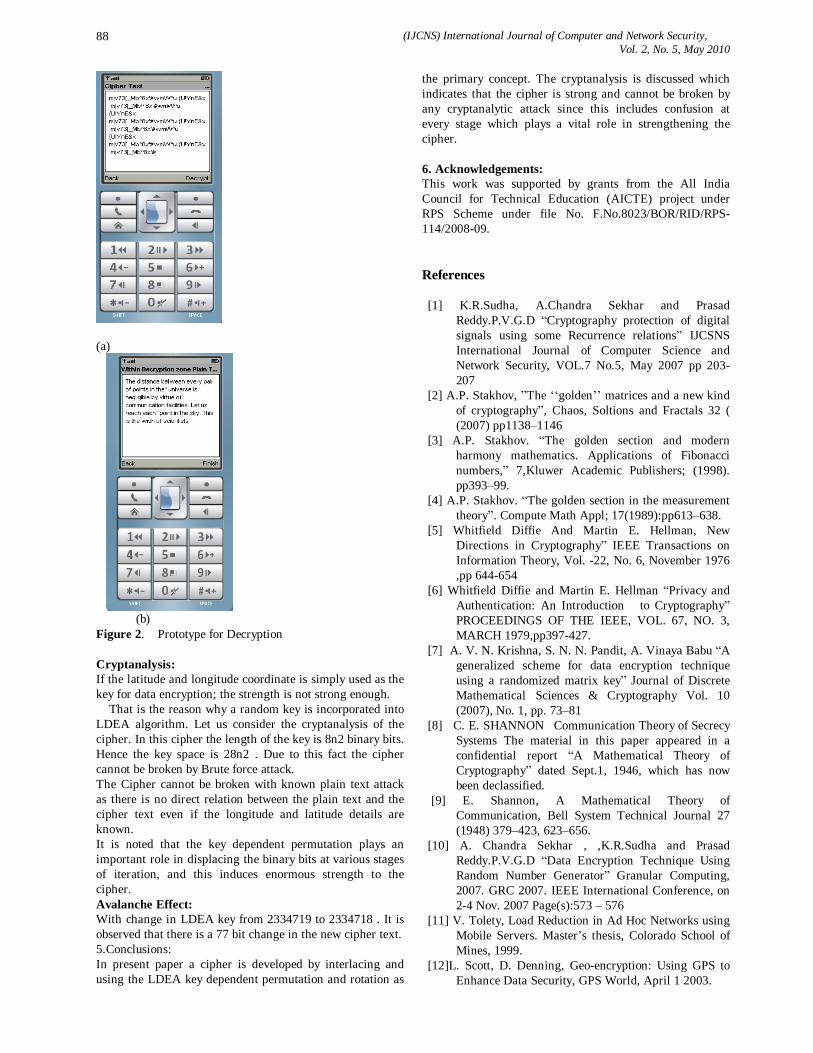
(IJCNS) International Journal of Computer and Network Security, Vol. 2, No. 5, May 2010
88
(a)
(b) Figure 2. Prototype for Decryption Cryptanalysis: If the latitude and longitude coordinate is simply used as the key for data encryption; the strength is not strong enough. That is the reason why a random key is incorporated into LDEA algorithm. Let us consider the cryptanalysis of the cipher. In this cipher the length of the key is 8n2 binary bits. Hence the key space is 28n2 . Due to this fact the cipher cannot be broken by Brute force attack. The Cipher cannot be broken with known plain text attack as there is no direct relation between the plain text and the cipher text even if the longitude and latitude details are known. It is noted that the key dependent permutation plays an important role in displacing the binary bits at various stages of iteration, and this induces enormous strength to the cipher. Avalanche Effect: With change in LDEA key from 2334719 to 2334718 . It is observed that there is a 77 bit change in the new cipher text. 5.Conclusions: In present paper a cipher is developed by interlacing and using the LDEA key dependent permutation and rotation as
the primary concept. The cryptanalysis is discussed which indicates that the cipher is strong and cannot be broken by any cryptanalytic attack since this includes confusion at every stage which plays a vital role in strengthening the cipher. 6. Acknowledgements: This work was supported by grants from the All India Council for Technical Education (AICTE) project under RPS Scheme under file No. F.No.8023/BOR/RID/RPS-114/2008-09. References [1] K.R.Sudha, A.Chandra Sekhar and Prasad
Reddy.P.V.G.D “Cryptography protection of digital signals using some Recurrence relations” IJCSNS International Journal of Computer Science and Network Security, VOL.7 No.5, May 2007 pp 203-207
[2] A.P. Stakhov, ”The ‘‘golden’’ matrices and a new kind of cryptography”, Chaos, Soltions and Fractals 32 ( (2007) pp1138–1146
[3] A.P. Stakhov. “The golden section and modern harmony mathematics. Applications of Fibonacci numbers,” 7,Kluwer Academic Publishers; (1998). pp393–99.
[4] A.P. Stakhov. “The golden section in the measurement theory”. Compute Math Appl; 17(1989):pp613–638.
[5] Whitfield Diffie And Martin E. Hellman, New Directions in Cryptography” IEEE Transactions on Information Theory, Vol. -22, No. 6, November 1976 ,pp 644-654
[6] Whitfield Diffie and Martin E. Hellman “Privacy and Authentication: An Introduction to Cryptography” PROCEEDINGS OF THE IEEE, VOL. 67, NO. 3, MARCH 1979,pp397-427.
[7] A. V. N. Krishna, S. N. N. Pandit, A. Vinaya Babu “A generalized scheme for data encryption technique using a randomized matrix key” Journal of Discrete Mathematical Sciences & Cryptography Vol. 10 (2007), No. 1, pp. 73–81
[8] C. E. SHANNON Communication Theory of Secrecy Systems The material in this paper appeared in a confidential report “A Mathematical Theory of Cryptography” dated Sept.1, 1946, which has now been declassified.
[9] E. Shannon, A Mathematical Theory of Communication, Bell System Technical Journal 27 (1948) 379–423, 623–656.
[10] A. Chandra Sekhar , ,K.R.Sudha and Prasad Reddy.P.V.G.D “Data Encryption Technique Using Random Number Generator” Granular Computing, 2007. GRC 2007. IEEE International Conference, on 2-4 Nov. 2007 Page(s):573 – 576
[11] V. Tolety, Load Reduction in Ad Hoc Networks using Mobile Servers. Master’s thesis, Colorado School of Mines, 1999.
[12]L. Scott, D. Denning, Geo-encryption: Using GPS to Enhance Data Security, GPS World, April 1 2003.

(IJCNS) International Journal of Computer and Network Security, Vol. 2, No. 5, May 2010
89
[13] Geo-encryption protocol for mobile networks A. Al-Fuqaha, O. Al-Ibrahim / Computer Communications 30 (2007) 2510–25
[14] PrasadReddy.P.V.G.D, K.R.Sudha and S.Krishna Rao “Data Encryption technique using Location based key dependent Permutation and circular rotation” (IJCNS) International Journal of Computer and Network Security,Vol. 2, No. 3, March 2010 pp46-49
[15]PrasadReddy.P.V.G.D, K.R.Sudha and S.Krishna Rao Rao “Data Encryption technique using Location based key dependent circular rotation” Journal of Advanced Research in Computer Engineering, Vol. 4, No. 1, January-June 2010, pp. 27 – 30
Authors Profile
Dr Prasad Reddy P V G D, is a Professor of Computer Engineering with Andhra University, Visakhapatnam, INDIA. He works in the areas of enterprise/distributed technologies, XML based object models. He is specialized in scalable web applications as an enterprise architect. With over 20 Years of experience in filed of IT and teaching, Dr Prasad Reddy has developed a number of
products, and completed several industry projects. He is a regular speaker in many conferences and contributes technical articles to international Journals and Magazines with research areas of interest in Software Engineering, Image Processing, Data Engineering , Communications & Bio informatics
K.R.Sudha received her B.E. degree in Electrical Engineering from GITAM, Andhra University 1991.She did her M.E in Power Systems 1994. She was awarded her Doctorate in Electrical Engineering in 2006 by Andhra University. During 1994-2006, she worked with GITAM Engineering College and presently she is working as Professor in the
department of Electrical Engineering, Andhra University, Visakhapatnam, India.
P Sanyasi Naidu is currently working as Associate Professor in the Department of Computer Science and systems Engg., GITAM University, Visakhapatnam. He is pursuing his PhD in Andhra University under the guidance of Prof.Prasad Reddy.
(IJCNS) International Journal of Computer and Network Security, Vol. 2, No. 5, May 2010
90
Factors Identification of Software Process Model – Using a Questionnaire
Abdur Rahshid Khan1, Zia Ur Rehman2
1 Institute of Computing & Information Technology,
Gomal Univeristy Dera Ismail Khan, Pakistan Email: [email protected]
2 Institute of Information Technology,
Kohat University of Science and Technology (KUST), Kohat, Pakistan
Email: [email protected]
Abstract: this work is an attempt to identify factors that are critical to software process model for a software project. Diverse types of software engineers can get benefit to select a software process model during development of software project. A questionnaire was developed with the help of domain experts, cited literature and rules of thumbs. This was sent to 100 domain experts with highest qualification and a vast experience of the fields of various institutions in Pakistan. Experts’ opinions from 34 domain experts were received with remarkable comments and suggestions. This questionnaire will be used as a Knowledge Acquisition tool for ESPMS (Expert System for Software Process Model Selection); which will integrate the knowledge of experts of various domains, like Software Engineering, Artificial Intelligence and Project Management. This questionnaire will lead to become a standard document of knowledge acquisition for selection of an appropriate software process model for a particular project. Further work is required to verify this tool through experts of various organizations (public and private) software houses within country and abroad.
Keywords: Software Engineering, Project Management, Artificial Intelligence, Expert System, Knowledge Acquisition Tool, Questionnaire
1. Study Background Explicit models of software evaluation date back to the
earliest projects developing large software systems in the 1950’s and 1960’s [1]-[2]. The main purpose of early life cycle models was to provide a conceptual scheme for managing the development of software system. Since the 1960’s descriptions of the classic software life cycle have appeared e.g., [1, 2, 3, 4 & 5].
If software is not a product, then software development is not a product. It cannot be. If the true product is not the software but the knowledge contained in the software, then software development can only be a knowledge acquisition activity. Translating that Knowledge into a specific language form known as “code” [7]. Knowledge is crucial resource of each organization and therefore it will be carefully managed. Knowledge is intensive in business areas. Knowledge is a mandatory source of business success [6].
Building and running corporate-wide knowledge management systems in the domain of Software Engineering is an idea that was initiated about 20 years ago [8]. There are two types of knowledge, tacit knowledge and explicit knowledge. Tacit knowledge is personal knowledge embedded in personal experience and is shared and exchanged through direct, face-to-face contact. Explicit knowledge is formal or semi-formal knowledge that can be packaged as information [6].
In article [6], author defined “Knowledge Management” (KM) as human resource management activities, such as hiring new staff or to train staff in order to increase the company’s capacities. The goal of KM is to improve organizational skills of all levels of the organization (individual, group, division, organization) by better usage of the resource knowledge. It is a management activity, and as such is goal oriented, planned and monitored.
The three laws for process are: (1) Process only allows us to do things we already know how to do. (2) We can only define software processes at two levels: too vague or too confining. (3) The very last type of knowledge to be considered as a candidate for implementation into an executable software system is the knowledge of how to implement knowledge into an executable software system. Author also focuses attention, that there are several problems in defining process in industry [7].
Comperative Study of Software Process Models Software process is a framework for the tasks that are
required to build high quality software [9]. A descriptive model describes the history of how a
particular software system was developed [4 & 13]. Prescriptive models are used as guidelines or frameworks
to organize and structure how software development activities should be performed, and in what order. Prescriptive models are also used to package the development tasks and techniques for using a given set of software engineering tools or environment during a development project. Descriptive life cycle models, characterize how particular software systems are actually developed in specific settings [3 & 4].
(IJCNS) International Journal of Computer and Network Security, Vol. 2, No. 5, May 2010
91
In order to ensure that cost-effective, quality systems are developed which address an organization’s business needs, developers employ some kind of system development Process Model to direct the project’s lifecycle [10]. To solve actual problems in an industry setting, a software engineer or a team of engineers must incorporate a development strategy that encompasses the process, methods, and tools layers and the generic phases [9].
Software process models often represent a networked sequence of activities, objects, transformations, and events that embody strategies for accomplishing software evolution. Software process networks can be viewed as representing multiple interconnected task chains. Task chains can be employed to characterize either prescriptive or descriptive action sequences. Prescriptive task chains are idealized plans of what actions should be accomplished, and in what order [11].
Some of the important models have been described in the following paragraphs.
The Linear Sequential Model, The linear sequential model, sometimes called the Classic or Waterfall model, proposed by Winsten Royce [11]. The linear sequential model suggests a systematic, sequential approach to software development that begins at the system level and progresses through analysis, design, coding, testing, and support [9].
Waterfall Model has some criticisms as: • Real projects rarely follow the sequential flow that the
model proposes. • At the beginning of most projects there is often a great
deal of uncertainty about requirements and goals, and it is therefore difficult for customers to identify these criteria on a detailed level. The model does not accommodate this natural uncertainty very well.
• Blocking state: means in this model some project team members must wait for other members of the team to complete dependant tasks.
• Developing a system using the Waterfall Model can be a long, painstaking process that does not yield a working version of the system until late in the process [10].
The Prototyping Model: A customer defines a set of general objectives for software but does not identify detailed input, processing, or output requirements. In these, and many other situations, a prototyping paradigm may offer the best approach [9 &11].
There are a few different approaches that may be followed when using the Prototyping Model [10]:
• Creation of the major user interfaces without any substantive coding in the background in order to give the users a “feel” for what the system will look like,
• Development of an abbreviated version of the system that performs a limited subset of functions; development of a paper system.
• Use of an existing system or system components to demonstrate some functions that will be included in the developed system.
Criticisms of the Prototyping Model generally fall into the following categories [10]:
• Prototyping can lead to false expectations. • Prototyping can lead to poorly designed systems. The RAD Model: Rapid Application Development
(RAD) is an incremental software development process model that emphasizes an extremely short development life cycle. It is a component-based construction, but high speed linear sequential. If requirements are well understood and project scopes constrained, the RAD process enables a development team to create “a fully functional system” with in very short time periods (e.g., 60 to 90 days) [9 & 11].
The RAD approach has drawbacks [9]: • Large and scalable projects require sufficient human
resources. • RAD requires developers and customers who are
committed to the rapid-fire activities necessary to get a system complete in specified time. If commitment is lacking from either constituency, RAD project will fail.
• If a system cannot be properly modularized, building the components necessary for RAD will be problematic.
• If high performance is issue and performance is to be achieved through tuning the interfaces to system components, the RAD approach may not work.
• RAD is not appropriate when technical risks are high. This occurs when a new application makes heavy use of new technology or when the new software requires a high degree of interoperability whit existing computer programs.
Evolutionary Software Process Model: Evolutionary models are iterative, which is one of the modern software development processes. Evolutionary models enable software engineers to develop increasingly more complete versions of the software [9 & 11].
Incremental Models: It combines elements of the linear sequential model applied respectively with the iterative philosophy of prototyping. First increment is often a core product. It is iterative in nature [5 & 9].
The Spiral Model: The spiral model, proposed by [3], is an evolutionary software process model that couples the iterative nature of prototyping with controlled and systematic aspects of the linear sequential model. A spiral model is divided into a number of framework activities, also called tasks or regions [9 & 11].
The Win-Win Spiral Model: The Customer wins by getting the system or product that satisfy the majority of the customer’s needs and the developer wins by working to realistic and achievable budgets and deadlines. Boehm’s WINWIN spiral model [12] defines a set of negotiation activities at the beginning of each pass around the spiral.
Criticism of a spiral model: The risk assessment component of the Spiral Model provides both developers and customers with a measuring tool that earlier Process Models do not have. The measurement of risk is a feature that occurs every day in real-life situations but (unfortunately) not as often in the system development industry. The practical nature of this tool helps to make the
(IJCNS) International Journal of Computer and Network Security, Vol. 2, No. 5, May 2010
92
Spiral Model a more realistic Process Model than some of its predecessors.
The Concurrent Development Model: The concurrent development model is also called concurrent engineering, [12]. The concurrent process model defines a series of events that will trigger transitions from state to state for each of the software engineering activities. A system and component activities occur simultaneously and can be modeled using the state-oriented approach described previously. Each activity on the network exists simultaneously with other activities [5, 9 & 11].
Component-Based Development: Object-Oriented technologies provide the technical framework for a component-based process model for Software Engineering [5, 9 & 11]. A general criticism of the Component-Based Model is that it is limited for use in object-oriented development environments. Although this environment is rapidly growing in popularity, it is currently used in only a minority of system development applications [10].
1.1 Creating and Combining Models: In many cases, parts and procedures from various Process
Models are integrated to support system development. This occurs because most models were designed to provide a framework for achieving success only under a certain set of circumstances. It is sometimes necessary to alter the existing model to accommodate the change in circumstances, or adopt or combine different models to accommodate the new circumstances. The selection of an appropriate Process Model hinges primarily on two factors: organizational environment and the nature of the application. Frank Land, from the London School of Economics, suggests that suitable approaches to system analysis, design, development, and implementation be based on the relationship between the information system and its organizational environment. Four categories of relationships are identified: The Unchanging Environment, the Turbulent Environment, the Uncertain Environment, and the Adaptive Environment [10].
1.2 Expert Systems Application For decision making and for problem solving Expert
System tools are used, which is Artificial Intelligence tool, they have ability to imitate the reasoning of human expert with in a specialized area [14]. Now in various areas such as computer science, agriculture, engineering, geology, space technology, medicine, etc expert systems are being used and developed (Durken 1990). The knowledgebase component of expert system is consists of human experts’ knowledge. The most difficult task is to acquire knowledge from experts and identification of problem in the development of expert systems [7, 8]. Interview, observation analysis, case study analysis, questionnaire, protocol analysis are the some knowledge acquisition techniques to acquiring knowledge and expertise in domain experts [14, 15, 16 & 17].
1.3 Knowledge Acquistion Capturing knowledge source from expertise is known as
knowledge acquisition technique. There are different sources from which knowledge can be acquired such as human experts, books, journals, reports, databases and other computer system [14]. The process through which knowledge engineers extract knowledge called Knowledge Acquisition [18]. Knowledge acquisition process is the first phase to develop an expert system [18]. There are some difficulties in during knowledge acquisition process i.e. sometime problem is not very clear to knowledge engineers, knowledge engineers have lack of knowledge in particular domain, sometime experts are not available in particular domain [16 & 18].
There are several reasons for employing an expert system such as [14]:-
§ Replacement of human expert § Assistant to human expert § Transfer of expertise to novice
From literature study it is revealed that there are a number of knowledge acquisition techniques exist, such as questionnaire, protocol analysis, Interview (structured and unstructured interview), case study analysis, observation analysis, simulation and prototyping [14 & 15).
Depending upon the nature of the problem, need, situation and domain experts, different acquisition techniques can be used accordingly. If the domain experts can easily be accessed, an interview is the best technique. If the expert are far-away from access of knowledge engineers or experts are much busy, then questionnaire is the most suitable tool. Similarly, if the target problem is complex, multiple techniques can be adopted.
2. Problem Domain Knowledge acquisition process was started from
identification of critical factors that affect directly or indirectly the process models, being critical in selection of appropriate software process model to software engineers. This tool will be used in ESPMS (Expert System for Software Process Model Selection), which is available free of cost.
Literature study reveals that research has been conducted on different phases of software process models, such as requirement analysis and specification, planning of software project, System Design and Architectural Design etc but there is no proper guidance for novice software designer and engineer, how to select a process model for a particular situation.
Ref [7] described the three laws of software process and also highlighted that there are several problems in defining a process in industry. Author also highlights rule of process bifurcation (Software process rules that are stated in terms of two levels: a general statement of the rule, and a specific detailed example), and the dual hypothesis of knowledge discovery (we can only “discover” knowledge in an environment that contains that knowledge). Ref [6] stated overall objective of Learning Software Organization (LSO)

(IJCNS) International Journal of Computer and Network Security, Vol. 2, No. 5, May 2010
93
is to improve software processes and products according to the strategic goals of the organization. Knowledge Management (KM) was defined, because KM is prerequisite of learning organization. Ref [19] stated that there is still lacking integration of software process modeling and software process measurement by software engineers. Language construct is used to better understand the process modeling technique. The Attribute Grammar (AG) approach to realize modeling of software processes modeling in language construct is based on its specification and automatic construction of language-based editors. Ref [20] Build Knowledge Analysis System (KANAL), which relates pieces of information in process models among themselves and to the existing Knowledge Base (KB), analyzing how different pieces of input are put together to achieve some effect. It builds interdependency models from this analysis and uses them to find errors and propose fixes. Ref [21] Recent research in software engineering has moved away from this linear approach of the life cycle in order to take account of dependencies between decisions taken in different parts of the development and to allow methods to be selected during developments which are appropriate to address problems that arise. The most advanced approach is the spiral model proposed by Boehm [3]. The major research project on KBS methodology is the KADS (Knowledge Acquisition and Design System). KADS proposes that knowledge modelling should pass through five stages: (Data, Conceptual Model, Design Model, Detailed Design Model, and Implementation). The Conceptual Model is further divided into a four layer knowledge model where each successive layer interprets the description of the lower layer: static domain knowledge, knowledge sources, task, and strategic knowledge. The major difficulty with advice on maintenance is that there is very little data or published experience on maintaining KBS. Two main properties directly influence the maintainability of a KBS. (1) The homogeneity of the maintained representation: (2) the predictability of the representation.
3. Approach In this research we are introducing the tool (i.e. a
questionnaire) for knowledge acquisition process to solve a selected problem. During development of this Knowledge Acquisition tool, following steps were adopted:
A). Selection of Domain Experts (B), Design and Distribution of Questionnaire and (C) Analysis and Findings.
3.1 Selection of Domain Experts Knowledge Base (collection of expert knowledge) is
critical and important component of the expert system [22]. The questionnaire was properly evaluated by domain
experts, which will lead to become a standard document for selection of appropriate software process model.
In Pakistan SE and AI are used mostly for research in Education, that’s why this questionnaire was distributed in various Higher Education Commission (HEC) recognized
universities of Pakistan. 100 domain experts along with detailed about them were found in 124 universities of Pakistan. See Table I for detail.
3.2 Design and Distribution of Questionnaire Extracting experts’ opinion to develop standard criteria
for factors that can affect software process model’s performance is the main purpose of this questionnaire. Questionnaire was the tool through which we could solicit experts’ opinion. A total of 99 questions (parameters) were identified, which were grouped into 11 main factors. Five fuzzy variables scales were defined, like, 5=Strongly Agree (Critical to process’s performance), 4 = Agree (Important to process’s performance), 3= Neutral (Helpful to process’s performance), 2= Disagree (Minimally affects process’s performance), 1= Strongly Disagree (Do not affect process’s performance).
We designed the questionnaire in such a way that the respondent have to rank the importance of factor regarding to its objective. Among 100 domain experts we received 34 experts’ opinions with valuable and remarkable suggestions.
Table 1: Experts Detail with their Responses
Experts’ Charac. Gender Designation Degree Subject
Specialty Demographic
Categorical Responses
Male: 30 Professor: 4 PhD: 4 Software Engineering: 20
Federal: 10
Female:4 Associate Professor: 8
M.Phil/MS:12
Artificial Intelligence: 8
Sindh:0
- Assistant Professor: 9
MCS/ MSc: 12
Software Project Management: 6
Punjab:4
- - Lecturers: 7 BCS (Hons): 6 - NWFP:10
- - Teachers: 6 - - Baluchistan: 10
- - - - - Azad Jammu & Kashmir: 0
- - - - - Total: 34 34 34 34 34 34
3.3 Analysis and Findings SPSS was used to analyze the collected facts. Table 2
shows the summary of questionnaire distribution.
Table 2: Questionnaire Distribution Medium Questionnaire
Distributed Responses %age
Through Email 60 20 33.33
Through Post 28 9 32.14
Through By hand 12 4 33.33
Total 100 34 34 The questionnaire was resulted in 11 main groups with 84
questions after repeatedly contact with the domain experts. Statistical analysis showed that System Integration &
Testing, User Community & Unit Development, Software Integration & Testing were the most important factors among rest of the main factors. See Table 3 for detail.

(IJCNS) International Journal of Computer and Network Security, Vol. 2, No. 5, May 2010
94
The ranking of factors were also helpful in determining the weights of the various factors, which influence the decision making process.
Table 3: Response Summary for Affect on Proces’
Performance (Total Reponses N: 34, 5= Critical Affects, 1=Do not Affect)
Main Groups of Factors Mean Std. Deviation
System Integration and Testing 3.8941 1.1494 User Community 3.4510 1.1441 Unit Development, Software Integration &
Testing 3.7426 1.0890 Implementation & Maintenance 3.7904 1.0881 Project Type and Risk Management 3.7941 1.0184 Validation and Verification 3.8168 0.9981 Quality Assurance and Quality Control 3.8333 0.9774 Requirement Analysis and Specification 3.8407 0.9762 System Design and Architectural Design 3.8848 0.9613 Project Team 3.8445 0.9565 Documentation 4.1823 0.8577
Table 4 depicts weights assigned to the main factors. In
weight criteria documentation, system integration and testing and validation and verification were the most important factors among rest of the main factors.
Table 4: Weight Assignment to main factors
S.No Main Groups of Factors Weights
1 Documentation 0.1041 2 System Integration and Testing 0.0971 3 Validation and verification 0.0969 4 System Design and Architectural Design 0.0956 5 Quality Assurance and Quality Control 0.0952 6 Project Team 0.0923 7 Implementation & Maintenance 0.0915
8 Requirements Analysis And Specification 0.0914
9 Project Type and Risk Management 0.0849
10 Unit Development, Software Integration & Testing 0.0793
11 User Community 0.0718 Total weight: 1.0000
After calculation of mean and standard deviation of main factors, we calculated mean and standard deviation of each and every sub-factor (questions).
4. Conclusions and Future Recommendation Each and every factor was properly analyzed, means and
standard deviations were calculated of each factors with the help of SPSS. Weights of the main factors were evaluated. Overall score will be calculated at run time through summation function, which will be used for ranking in the selection of a process model. (See my research thesis for detail).
It is further recommended that this questionnaire is not in final shape which will be distributed in local (Pakistan) and international software houses. This questionnaire is not final standard tool for selection of an appropriate software process
model but it is just an approach, guideline and helping tool for software engineer in selection of process model. This questionnaire may become a standard Knowledge Acquisition tool for Expert System development.
Figure 1: Knowledge Elicitation Process of a Software Process Model Selection
References
[1] Hoiser, W.A., “Pitfalls and Safegaurds in Rea-Time Digital Systems with Emphasis on programming,” IRE Trans. Engineering Management, EM-8, June 1961.
[2] Royce, W. W., “Managing the Development of Large Software Systems,” Proc. 9th. Intern. Conf.Software Engineering, ,IEEE Computer Society, 1987 ,328-338 Originally published in Proc. WESCON, 1970.
[3] Boehm, B., “A Spiral Model for Software Development and Enhancement,” Computer, Vol. 21, no. 5, May 1988, pp. 61-72
[4] Scacch i W., Process Models in Software Engineering, Institute for Software Research, University of California, Irvine February 2001.
[5] Sommerville I., Software Engineering 5th Edition, 2000 [6] Ruhe G. (2000), “Learning Software Organizations”,
Fraunhofer Institute for Experimental Software Engineering (IESE).
[7] Caesar & Cleopatra (2004), “Chapter 1,The Nature of Software and the Laws of Software Process” www.ism-journal.com/ITToday/AU1489_C01.pdf, CRC Press, LLC.
[8] Basili V.R, Zelkowitz, M. V. McGarry, F. Page, S. Waligora, R. Pajerski. SEL’s Software Process Improvement Program, IEEE Software, vol. 12, November, pp 83-87, 1995.
[9] Pressman R. S, Software Engineering a Practitioner’s Approach, Fifth Edition, 2001.
[10] SUNY 1988 , “ A Survey of System Development Pr ocess Models” , CTG.MFA – 00, Center for Technology in Government, University at Albany.
Questionnaire
Characteristics of Software Process Models
Factors Identification
Domain Experts (Books, Journals, Databases, Reports, Internet etc)
Reference Knowledge
Analyzed Facts (Knowledge Elicitation)

(IJCNS) International Journal of Computer and Network Security, Vol. 2, No. 5, May 2010
95
[11] Reddy A. R. M, Govindarajulu P., Naidu M., A Process Model for Software Architecture, IJCSNS, VOL.7 No.4, April 2007.
[12] Davis, A. and Sitaram P., “A Concurrent Process Model for Software Development,” Software Engineering Notes, ACM Press, vol. 19, n0. 2, April 1994, pp. 38-51
[13] Curtis, B., H. Krasner, and N. Iscoe, A Field Study of the Software Design Process for Large Systems, Communications ACM, 31, 11, 1268-1287, November, 1988.
[14] Awad, E.M. “Building Experts Systems: Principals, Procedures, and Applications,” New York: West Publishing Company. 1996.
[15] Durkin, J. “Application of Expert Systems in the Sciences,” OHIO J. SCI. Vol. 90 (5), pp. 171-179, 1990.
[16] Medsker, L. and Liebowits, J. “Design and Development of Experts Systems and Neural Networks,” New York: Macmillan Publishing Company, 1987.
[17] Sagheb-Tehrani, M.“The design process of expert systems development: some concerns, Expert system,” Vol. 23 (2), pp. 116-125, 2006.
[18] Wagner, W.P., Najdawi, M.K., Chung, Q.B “Selection of Knowledge Acquisition techniques based upon the problem domain characteristics of the production and operations management expert systems,” Expert system, vol. 18 (2), pp. 76-87, 2001.
[19] Atan, R. Abd, A. A. Ghani, M. H.S. & Mahmod, R. “ Software Process Modelling using Attribute Grammar” University Putra Malaysia, Serdang, Selangor Darul Ehsan, Malaysia, IJCSNS International Journal of Computer Science and Network Security, VOL.7 No.8, August 2007.
[20] Kim, J. & Gil, Y. “Knowledge Analysis on Process Models”, Information Sciences Institute University of Southern California, International Joint Conference on Artificial Intelligence (IJCAI-2001), Seattle, Washington, USA, August 2001.
[21] Wilson, “Knowledge Acquisition: The current position”, Science and Engineering Research Council Rutherford Appleton Laboratory.
[22] Lightfoot,J.M.” Expert knowledge acquisition and the unwilling experts: a knowledge engineering perspective,” Expert system, vol. 16(3), pp.141-147, 1999.
[23] Futrell R. T., Shafer L. I, Shafer D. F, “Quality Software Project Management”, Low Price Edition, 2004.
[24] Anderson S., & Felici M., “Requirement Engineering Questionnaire”, Version 1.0, Laboratory for Foundation of Computer Science, Edinburgh EH9 3JZ, Scotland, UK (2001).
[25] Skonicki M., “QA/QC Questionnaire for Software Suppliers”, January 2006.
[26] Energy U. S. D., “Project Planning Questionnaire”, www.cio.energy.gov/Plnquest.pdf (last access, 04 August 2009)
[27] Liu & Perry (2004), “On the Meaning of Software Architecture, Interview Questionnaire, (July, 2004), Version 1.2
Authors Profile
Abdur Rashid Khan is presently working as an Associate Professor at ICIT, Gomal University D.I.Khan, Pakistan. He has received his PhD degree from Kyrgyz Republic in 2004. His research interest includes AI, Software Engineering, MIS and DSS. Zia Ur Rehman is currently pursuing his MS degree in Computer Science from the Institute of Information Technology, Kohat University of Science & Technology (KUST), Kohat, Pakistan. His area of interest includes Software Engineering, Artificial Intelligence/Expert System, Databases and Data Mining.

(IJCNS) International Journal of Computer and Network Security, Vol. 2, No. 5, May 2010
96
Appendix: (Questionnaire) A SURVEY ON FACTORS AFFECTING TO SELECT A SOFTWARE DEVELOPMENT PROCESS MODEL Respondent’s Name: _______________ Qualification: _________ Designation: ______________ Address/University: __________________________
5= Strongly Agree 4= Agree 3=Neutral 2= Disagree 1=Strongly Disagree
Critical to Process’s Performance
Important to Process’s Performance
Helpful to Process’s performance
Minimally affects Process’s performance
Do not affect Process’s performance
ATTRIBUTES LEVELS 5 4 3 2 1
1 Requirements Analysis And Specification
1.1 Are the requirements precisely defined, well defined and well known? 1.2 Are requirements sufficient to help you understand the problem structure? 1.3 Are the requirements defined early in the cycle [23]? 1.4 Are the requirements will change often in the cycle [23]? 1.5 Is there need to demonstrate capability proof of concept [23]? 1.6 Does the requirement indicate a complex system/simple system [23]? 1.7 Is there appropriate procedure prepared for cost/benefit analysis [24]? 1.8 Does the requirements phase meet the requirements methodology [24]? 1.9 Are you sensible to organizational and political factors which influence requirements sources while eliciting requirements [24]? 1.10 Have you reuse requirements from other systems which have been developed in the same application area [24]? 1.11 How do you handle continuous requirements change [24]? 1.12 Does any risk analysis are performed on requirements [24]? 1.13 Is the requirements document easy to change [24]? 1.14 Do you define Cost-effectiveness criteria [24]? 1.15 Do you identify accuracy and completeness risks on the requirements analysis [24]? 1.16 Are rules established on handling inaccurate and incomplete data [24]? 1.17 Do you cross-check operational and functional requirements against safety (or security, availability, etc.) requirements [24]? 1.18 Are specifications kept up-to-date and controlled [25]? 1.19 Are your software-product versions reviewed for conformity to customer’s specifications [25]? 1.20 Are the versions reviewed for compliance to quality requirements before submission for customer approval [25]? 2 Project Team 2.1 Does the majority of team members new to the problem domain [23]? 2.2 Does the majority of team members new to the technology domain [23]? 2.3 Is there need to train to project team [23]? 2.4 Is the team more comfortable with structure than flexibility [23]? 2.5 Will the project manager closely track the team’s progress [23]? 2.6 Is ease of resource allocation important [23]? 2.7 Does the team accept peer reviews and inspections, management/customer reviews, and mile-stones [23]? 3 User Community 3.1 Will the availability of the user representatives be restricted or limited during the life cycle [23]? 3.2 Are the user experts in the problem domain [23]? 3.3 Do the users want to be involved in all phases of the life cycle [23]? 4 Project Type and Risk 4.1 Dose the customer want to track project progress [23]? 4.2 Does the project identify a new product direction for the organization [23]? 4.3 Is the project a system integration project [23]? 4.4 Is the project an enhancement to an existing system [23]? 4.5 Is the funding for the project expected to be stable throughout the life cycle [23]? 4.6 Is the product expected to have a long life in the organization [23]? 4.7 Is high reliability a must [23]? 4.8 Is the system expected to be modified perhaps in ways not anticipated, post-deployment [23]? 4.9 Is the schedule constrained [23]? 4.10 Are the modules interfaces clean [23]? 4.11 Are reusable components available [23]?
INSTRUCTIONS Different software process model exist, to select one for a particular software depends upon the nature of project, problem structure, risk involve, budget estimation, goals & objectives of the project etc. As an EXPERT in this area, you are requested to examine each item in terms of suitability and then to explain the degree of your agreement to each item whether, in your opinion, it would measure the factors affecting the selection of software development process model and to what extent. You may recommend new & delete unnecessary items from the existing scale. Your in-time response will highly be appreciated. Please, use the scale below to mark (P) your responses in the area provided.
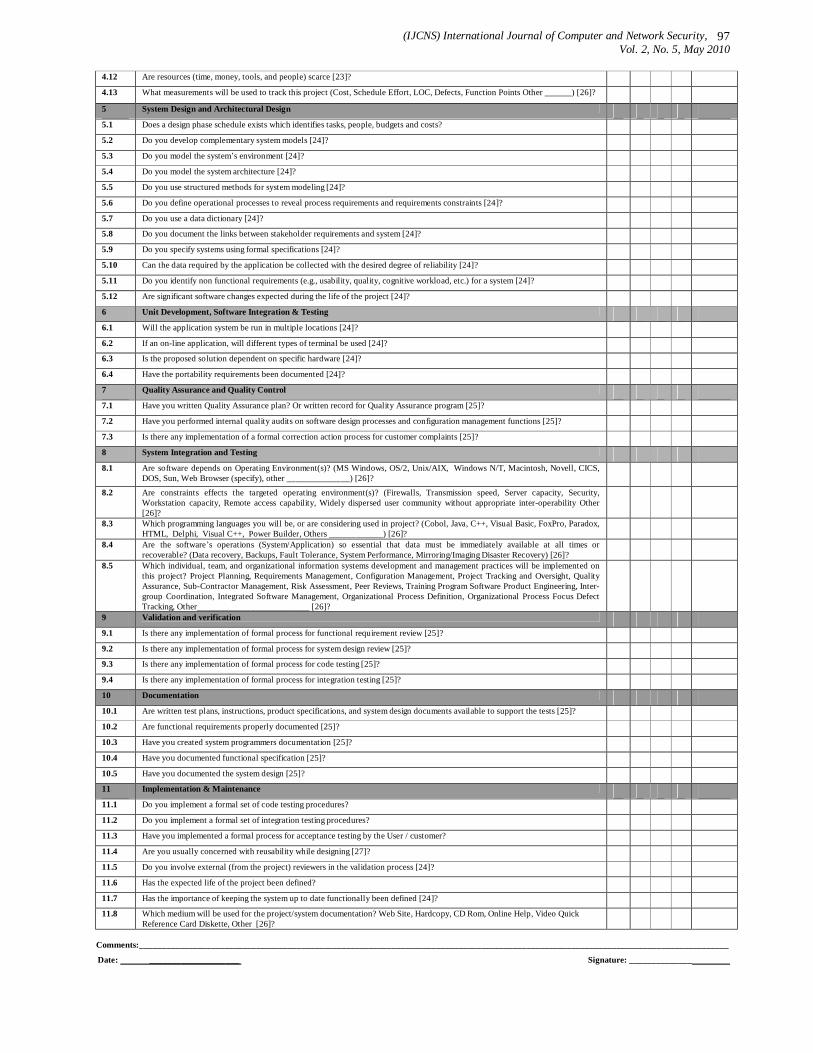
(IJCNS) International Journal of Computer and Network Security, Vol. 2, No. 5, May 2010
97
4.12 Are resources (time, money, tools, and people) scarce [23]? 4.13 What measurements will be used to track this project (Cost, Schedule Effort, LOC, Defects, Function Points Other ______) [26]? 5 System Design and Architectural Design 5.1 Does a design phase schedule exists which identifies tasks, people, budgets and costs? 5.2 Do you develop complementary system models [24]? 5.3 Do you model the system’s environment [24]? 5.4 Do you model the system architecture [24]? 5.5 Do you use structured methods for system modeling [24]? 5.6 Do you define operational processes to reveal process requirements and requirements constraints [24]? 5.7 Do you use a data dictionary [24]? 5.8 Do you document the links between stakeholder requirements and system [24]? 5.9 Do you specify systems using formal specifications [24]? 5.10 Can the data required by the application be collected with the desired degree of reliability [24]? 5.11 Do you identify non functional requirements (e.g., usability, quality, cognitive workload, etc.) for a system [24]? 5.12 Are significant software changes expected during the life of the project [24]? 6 Unit Development, Software Integration & Testing 6.1 Will the application system be run in multiple locations [24]? 6.2 If an on-line application, will different types of terminal be used [24]? 6.3 Is the proposed solution dependent on specific hardware [24]? 6.4 Have the portability requirements been documented [24]? 7 Quality Assurance and Quality Control 7.1 Have you written Quality Assurance plan? Or written record for Quality Assurance program [25]? 7.2 Have you performed internal quality audits on software design processes and configuration management functions [25]? 7.3 Is there any implementation of a formal correction action process for customer complaints [25]? 8 System Integration and Testing 8.1 Are software depends on Operating Environment(s)? (MS Windows, OS/2, Unix/AIX, Windows N/T, Macintosh, Novell, CICS,
DOS, Sun, Web Browser (specify), other ______________) [26]?
8.2 Are constraints effects the targeted operating environment(s)? (Firewalls, Transmission speed, Server capacity, Security, Workstation capacity, Remote access capability, Widely dispersed user community without appropriate inter-operability Other [26]?
8.3 Which programming languages you will be, or are considering used in project? (Cobol, Java, C++, Visual Basic, FoxPro, Paradox, HTML, Delphi, Visual C++, Power Builder, Others ____________) [26]?
8.4 Are the software’s operations (System/Application) so essential that data must be immediately available at all times or
recoverable? (Data recovery, Backups, Fault Tolerance, System Performance, Mirroring/Imaging Disaster Recovery) [26]?
8.5 Which individual, team, and organizational information systems development and management practices will be implemented on this project? Project Planning, Requirements Management, Configuration Management, Project Tracking and Oversight, Quality Assurance, Sub-Contractor Management, Risk Assessment, Peer Reviews, Training Program Software Product Engineering, Inter-group Coordination, Integrated Software Management, Organizational Process Definition, Organizational Process Focus Defect Tracking, Other_________________________ [26]?
9 Validation and verification 9.1 Is there any implementation of formal process for functional requirement review [25]? 9.2 Is there any implementation of formal process for system design review [25]? 9.3 Is there any implementation of formal process for code testing [25]? 9.4 Is there any implementation of formal process for integration testing [25]? 10 Documentation 10.1 Are written test plans, instructions, product specifications, and system design documents available to support the tests [25]? 10.2 Are functional requirements properly documented [25]? 10.3 Have you created system programmers documentation [25]? 10.4 Have you documented functional specification [25]? 10.5 Have you documented the system design [25]? 11 Implementation & Maintenance 11.1 Do you implement a formal set of code testing procedures? 11.2 Do you implement a formal set of integration testing procedures? 11.3 Have you implemented a formal process for acceptance testing by the User / customer? 11.4 Are you usually concerned with reusability while designing [27]? 11.5 Do you involve external (from the project) reviewers in the validation process [24]? 11.6 Has the expected life of the project been defined? 11.7 Has the importance of keeping the system up to date functionally been defined [24]? 11.8 Which medium will be used for the project/system documentation? Web Site, Hardcopy, CD Rom, Online Help, Video Quick
Reference Card Diskette, Other [26]?
Comments:___________________________________________________________________________________________________________________________________
Date: ____________________ Signature: ______________
(IJCNS) International Journal of Computer and Network Security, Vol. 2, No. 5, May 2010
98
MOBINA: A Novel DBA Method Based on Second Price Auction in Ethernet Passive Optical Network
AR. Hedayati1, M.N Feshaaraki1 ,K. Badie2 , A. Khademzadeh2 and M. Davari3
1Department of Computer Engineering, Science and Research Branch, Islamic Azad University(IAU) Hesarak ,poonak SQ, Tehran, Iran.
[email protected] 2Iran Telecom Research Center North kargar str, Tehran, Iran
3Department of Computer Engineering, Central Tehran Branch, Islamic Azad University Hamila Blv, poonak SQ, Tehran, Iran.
Abstract: Ethernet Passive Optical Network(EPON) is one of the best solutions for implementing the next generation access networks. One of the key issue in these network is bandwidth allocation to provide the quality of service for the End users.In this paper, we present a Novel Dynamic Bandwidth Allocation (DBA) method based on Second Price Auction in Ethernet Passive Optical Network. Results have shown improvements of the packet loss rate, throughput rate, and utilization line of our method when compared with other methods.
Keywords: Ethernet Passive Optical Network, Dynamic Bandwidth Allocation, Second price auction, Quality of Services.
1. Introduction Ethernet Passive Optical Network is one of the most important solutions for implementing the next generation of access networks. High capacity and low cost of implementing are among the characteristics of this technology, which can provide the required quality service in spite of expansion the quantity of user and their requests to use different multimedia services [1]. An EPON system is a point-to-multipoint fiber optical network with no active elements in the transmission path from its source, i.e., an optical line terminal (OLT), to a destination, i.e., an optical network unit (ONU). It can use different multipoint topologies, such as bus, ring, tree, and different network architectures [2]. The most typical EPON architecture is based on a tree topology and consists of an OLT, a 1:N passive star coupler (or splitter/combiner), and multiple ONUs, as shown in Figure (1). The OLT resides in a central office (CO) that connects the access network to a metropolitan area network (MAN) or a wide area network (WAN), and is connected to the passive star coupler through a single optical fiber [2]- [5].
Figure 1. EPON’s Architecture
One of the main concerns in this network is bandwidth allocation to provide end users quality of service for using multimedia service. To solve this problem, there have suggested different static and dynamic bandwidth allocation methods [2], [4]. In this paper, along with studying bandwidth allocation methods in EPON, we present a novel method named MOBINA, based on Second Price Auction. The MOBINA can allocate the users required bandwidth righteously and with high profitability. The rest of this paper is organized as follows: In Section 2, we introduce related work of Bandwidth allocation methods in EPON. In section 3, we explain MOBINA method in details. In section 4, we present simulation results. In section 5, we conclude this paper.
2. Related work Bandwidth allocation methods are discussed as one of the most important QOS’s parameters in EPON [6]. In bandwidth allocating for each network unit, optical line terminal needs to provide some method based on the received bandwidth demands of optical network units and some allocation policies or service level agreements are in this content [7]. At present many methods are recommended, in general they classified in two general types: Static Bandwidth Allocation and Dynamic Bandwidth Allocation.
2.1 Static Bandwidth Allocation methods Each ONU is assigned with a constant bandwidth regardless to its actual bandwidth demand. As a result, the allocated bandwidth might either not be fully utilized, in the case of ONUs with light traffic requirement or not be adequate to accommodate heavy traffic load ONUs, resulting in both scenarios to inefficient bandwidth utilization rate. In contrast a dynamic MAC protocol could more successfully allocate bandwidth according to ONUs’ instantaneous buffer queue status increasing the bandwidth utilization rate [8]. Research initiatives in MAC protocol development over the years have attempted to enhance further bandwidth allocation of standardized PON topologies, tracing back to PONs and more intensively to more recent and lately deployed EPONs . In common to all these topologies, the feeder pathway is shared in the time domain, and as a result each ONU can utilize the whole upstream optical carrier
(IJCNS) International Journal of Computer and Network Security, Vol. 2, No. 5, May 2010
99
capacity for defined, according to network penetration, and in most cases flexible duration time-slots, assigned by the OLT [7].
2.2 Dynamic Bandwidth Allocation methods To increase bandwidth utilization, the OLT must dynamically allocate a variable timeslot to each ONU based on the instantaneous bandwidth demand of the ONUs. Given that QoS is the main concern in EPONs, these methods classified into DBA with QoS support, DBA without QoS support, and describe their characteristics and performances [11].
2.2.1 DBA without differentiated QoS support There are several DBA methods proposed for EPON which do not support differentiated services, such as IPACT [9], it employs a resource negotiation process to facilitate queue report and bandwidth allocation. The OLT polls ONUs and grants timeslots to each ONU in a round robin fashion. The timeslot granted to an ONU is determined by the queue status reported from that ONU. Therefore, the OLT is able to know the dynamic traffic load of each ONU and allocate the upstream bandwidth in accordance with the bandwidth demand of each ONU. So demanded bandwidth can be granted efficiently also there exists three different ways for the OLT to determine the granted efficiently also there exists three different ways for the OLT to determine the granted window size to allocate bandwidth so they introduced Fixed service, Gated service, Limited service as IPACT service discipline to demonstrate bandwidth allocation in this method . Development and improvement of this method is considered in IPACT GE [10], Estimation-based DBA [11] and IPACT with SARF [2]. Bandwidth guaranteed polling (BGP) is another DBA method proposed for providing bandwidth guarantees in EPONs [12]. In BGP, all ONUs are divided into two groups: bandwidth guaranteed and bandwidth non-guaranteed. The OLT performs bandwidth allocation through using couple of polling tables. The number of bandwidth units allocated to an ONU is determined by the bandwidth demand of that ONU, which is given by its SLA with a service provider. A bandwidth guaranteed ONU with more than one entry in the poling table has its entries spread through the table. This can reduce the average queuing delay because the ONU is polled more frequently. However, this leads to more grants in a cycle and thus requires more guard times between grants, which reduces channel utilization. Methods have been introduced for all best effort traffic is suitable.
2.2.2 DBA with differentiated QoS support
An EPON system is expected to deliver not only the best effort data traffic, but also real-time data traffic (e.g., voice and video) that have strict bandwidth, packet delay, and delay jitter requirements. In this subsection present several DBA methods that can provide differentiated QoS support for different types of data traffic in EPON. One of the most important methods in field is fair sharing with dual SLAs (FSD-SLA) proposed a fair sharing with dual SLAs (FSD-SLA) method, which employs dual SLAs in IPACT to manage the fairness for both subscribers and service
providers [13]. The primary SLA specifies those services whose minimum requirements must be guaranteed with a high priority. The secondary SLA describes the service requirements with a lower priority. This method first allocates timeslots to those services with the primary SLA to guarantee their upstream transmissions. After the services with the primary SLA are guaranteed, the next round is to accommodate the secondary SLA services. If the bandwidth is not sufficient to accommodate the secondary SLA services, the max-min policy is adopted to allocate the bandwidth with fairness. If there is excessive bandwidth, FSD-SLA will allocate the bandwidth to the primary SLA entities first and then to the secondary SLA entities, both by using max-min fair allocation. Another optimizing method for dynamic bandwidth allocation with differentiated QoS support is LSTP .during the waiting period and thus more accurately grants bandwidth to each ONU. For each class of traffic, LSTP estimates the data that arrive during the waiting period based on the data of this class that actually arrived in previous transmission cycles by using a linear predictor [14]. The bandwidth demand of an ONU is thus the reported queue length plus the estimation. The OLT arbitrates the upstream bandwidth using this estimation and reserves a portion of the upstream bandwidth for transmitting the estimated data in the earliest transmission cycle, thus reducing packet delay and loss. Other methods proposed for dynamic bandwidth allocation with differentiated QoS support are: COPS, HGP, DBAM and so forth [2].
3. The MOBINA DBA Method
The MOBINA is dynamic bandwidth allocation based on Second Price Auction. In this method, all bandwidth requests are sent to OLT by ONUs. OLT can make a dynamic and fair decision about bandwidth allocation by auction process. The steps of auction process and bandwidth allocation in the suggested method are as follows: Step 1: Kick-off the auction by OLT Step 2: Submit the bid by ONUs Step 3: Assess received bids by OLT Step 4: Schedule and allocate bandwidth to winners Step5: Update and go to next round of auction Figure (2) represents the block diagram of the MOBINA method.

(IJCNS) International Journal of Computer and Network Security, Vol. 2, No. 5, May 2010
100
Figure 2.Dialgue diagram of the MOBINA method As shown in Figure (2), in Step 1 a signal is sent from OLT to ONUs in order to ONUs send their requested bandwidth allocation to OLT for participation in an auction. In step 2 based on the MOBINA method, ONUs calculate their Bid amount based on two parameters of the requested bandwidth and the last time of bandwidth allocation by OLT to ONU, and send it to OLT. Equation (1) shows the sent Bid amount by ONUi to OLT.
( )( ) ( ), ( 1)onu onui i iBid t BRQ t LST t= β −
(1)
In Equation (1), onu
iBRQ is the total bandwidth amount that
has been requested by the users from ONUi and onuiLST Is
the Boolean parameter that shown the last time of ONUi received bandwidth service. Equation (2) shows ONUi requested bandwidth.
e
1
( ) ( )K
R qonui J
J
BRQ t BW t=
= ∑
(2)
In Equation (2), eR q
JBW is the bandwidth required by users connected to ONUi. Equation (3) shows the required bandwidth of each user.
Re ( )q P PJ J JJBW t m L P= × × (3)
In Equation (3), P
Jm is the number of requested packets to
send for user j. PJL is the length of requested packets to
send, and JP is the priority of the jth user. In MOBINA suggested method, the priority of all users linked to an ONU is the same and is equal to (1/j). In step 3, after receiving all the Bids based on second price auction, OLT will select ONUs that win in auction and will
send the result to ONUs. In step 4, ONU will allocate the requested bandwidth for each user according to the timing of auction winners, considering the maximum accessible bandwidth. Equation (4) shows bandwidth allocation by OLT.
( ) ( )
( )
0 ( )
onuBRQ t ONU wini ionuBW ti
ONU lossi
=
(4)
In step 5, OLT updates the onu
iLST value of all the ONUs that have received bandwidth service in time t and will send the respective ONU. Equation (5) shows the value of
onuiLST .
0 ( )( )
1 ( )
ionu
i
i
ONU winLST t
ONU loss
=
(5)
Finally, after sending onuiLST values, OLT holds for a time
in order to allocated bandwidth be released and the conditions for holding auction by OLT is provided.
4. Computer Simulations To measure the performance of each bandwidth allocation methods we designed an event-driven C++ based EPON simulator. NS-2 and C# software is used as a unique system to compare simulation results. In this article we use EPON structure, as shown in Figure (1), to measure QoS parameters. The parameters considered for simulation are as illustrated in Table (1):
Table 1: Simulation Parameters Parameters Symbol Value Number of ONUs N 16 Bit Rate Λ 5 to 57.5 MBit/s Two way delay fiber Tfiber 200 µs Processing Time Tproc 35 µs Packet Size B 15000Byte(30
Packets) Ethernet Overhead Beth 38 Byte Request Message Size Breq 570 Bit Upstream Bandwidth Ru 1 GBit/s Maximum Transition Window
Pmax 10 Packets
Guard Time Tg 5 µs Max cycling time TMax 2 ms Buffer capacity BQmax 10 Mbyte Guarantied Bandwidth BAga 60 MBit/s Interval traffic randomly Interval 50 µs-100 µs Traffic Type CBR
All the provided results in this section which will be introduced, are measured the QoS based on proposed approach in comparison with other methods, will be analyzed by some different charts with their quantities such

(IJCNS) International Journal of Computer and Network Security, Vol. 2, No. 5, May 2010
101
as delay, jitter, Throughput, Packet loss and Utilization rate . Figure (3) shows traffic packet delay. The proposed approach has less delay in comparison with the methods of bandwidth allocation without QoS, although in the previous methods of bandwidth allocation with different QoS, at the first place in this approach delay is more because of providing situation awareness for ONUs, nevertheless in the other times delay is much better.
Figure 3.The charts for average of packets Delay Also, Figure (4), shows the vector of The Average of Traffic Packet Jitter. This chart we see that BGP and FSD-SLA jitter range is higher than other methods. Albeit with increasing traffic load and good behavior of IPACT methods, they have good Jitter rather than the other methods . At the point of view in jitter charts, which is implied much better jitter ratio of proposed approach compared to the other methods.
Figure 4.The Charts for Average of Packet Jitter
In addition, The chart related to throughput and loss rate of this traffic Loads is shown in Figure (5) and (6). As a result of analyzing these charts that implied better and more sufficient throughput compared to the other methods that we mentioned completely. Also we can realize that packet lost is reduced by increasing traffic load.
Figure 5.The Charts for Throughput Rate
Figure 6 . The Charts for Packet Loss Rate
Finally, Figure (7) depicts the rate of utilization in EPON systems. This Fig demonstrates that increasing of traffic load has anonymous utilization compared to the best methods. MOBINA approach has the most rate of network Utilization. Albeit this subject, the behavior of this Approach was predictable. By increasing the traffic load to network, Utilization rate in other methods didn’t have any difference.
Figure 7.The Charts for Line Utilization rate
5. Conclusion Bandwidth allocation is a critical issue in the design of an EPON system. Since multiple ONUs share a common upstream channel, an EPON system must efficiently utilize the limited upstream bandwidth in order to meet the bandwidth demands and quality of service requirements of end users. In this article, MOBINA method optimizes the bandwidth limitation problem. The results of the simulations showed that in comparison to other methods, the proposed method offers better performance in terms of average packet loss ratio and throughput ratio. And as a result, we improve the overall network performance.
(IJCNS) International Journal of Computer and Network Security, Vol. 2, No. 5, May 2010
102
References [1] G. Kramer and G. Pesavento, "Ethernet passive optical
network (EPON):building a next-generation optical access network," IEEE Communications Magazine, pp. 66-73, 2002.
[2] J. Zhenga, T. Hussein, ”A survey of dynamic bandwidth allocation methods for Ethernet Passive Optical Networks ”, Elsevier Journal Optical Switching and Networking, pp. 151-162, 2009.
[3] A. Xiaofeng ,s. Abdallah , “On the fairness of dynamic bandwidth allocation schemes in Ethernet passive optical networks”, Elsevier journal of computer communications, pp. 2123-2135, 2008.
[4] H. Naser, H. Mouftah, “A joint-ONU interval-based dynamic scheduling algorithm for Ethernet passive optical networks”, IEEE/ACM Transactions on Networking ,pp. 889-899 , 2006.
[5] Z. J., "Efficient Bandwidth Allocation Method for Ethernet Passive Optical Networks," in Proceedings of IEE Communications, pp.464-468, 2006.
[6] X. Bai, A. Shami, C. Assi, Statistical Bandwidth Multiplexing in Ethernet Passive Optical Networks, in Proceedings of IEEE Global Telecommunications Conference, 2005.
[7] J. Zheng, H. T. Mouftah, "An Adaptive MAC Polling Protocol for Ethernet Passive Optical Networks", in Proceedings of IEEE ICC, pp. 1874-1878, 2005.
[8] B. Moon, “Emergency handling in Ethernet passive optical networks using priority-based dynamic bandwidth allocation”, in Proceeding of IEEE INFOCOM'08, pp. 1319_1327, 2008. .
[9] S. Bhatia, R. Bartos, IPACT with smallest available report first: A new DBA method for EPON, in Proceeding. of IEEE ICC'07, pp. 2168_2173, 2007.
[10] H. Song, B.-W. Kim, B. Mukherjee, Multi-thread polling: A dynamic bandwidth distribution scheme in long-reach PON, IEEE Journal on Selected Areas in Communications ,) pp. 134-142, 2009.
[11] Y. Zhu, M. Ma, “IPACT with grant estimation (IPACT-GE) scheme for Ethernet passive optical networks”, IEEE/OSA Journal of Lightwave Technology, pp. 2055-2063, 2008.
[12] M. Ma, Y. Zhu, T. Cheng, “A bandwidth guaranteed polling MAC protocol for Ethernet passive optical Networks”, in Proceeding of IEEE INFOCOM'03, pp. 22_31, 2003.
[13] A. Banerjee, G. Kramer, B. Mukherjee, “Fair sharing using dual service-level agreements to achieve open access in a passive optical network”, IEEE Journal on Selected Areas in Communications, pp. 32_44, 2006.
[14] Y. Luo, N. Ansari, “Limited sharing with traffic prediction for dynamic bandwidth allocation and QoS provisioning over EPONs”, OSA Journal of Optical Networking, pp.561_572, 2005 .
Authors Profile Alireza Hedayati:. received his B.Sc. and M.Sc. in Computer Hardware Engineering from Azad University of Tehran Central Branch and Tehran science and research branch in 2000 and 2003, respectively. He is currently studying Computer Hardware in his Ph.D. degree. His research interests include
Optical Networks, Next Generation Network, Network Management and QoS.
Mehdi N. Feshaaraki:. received his Ph.D. in computer Engineering from NSW university of Australia. He is currently associate professor in computer Engineering Department of IAU. . His research interests include Computer Networks, information and knowledge architecture.
Kambiz Badie:. received his B.Sc., M.,Sc, and Ph.D. in electronic engineering from the Tokyo Institute of Technology, Japan, majoring in Pattern Recognition & Arlificia1lntelligance. His major research interests are Machine Learning, Cognitive Modeling, and Systematic Knowledge Processing in general, and Analogical Knowledge Processing, Experience-Based
Modeling and Interpretative Modeling in particular with emphasis on ides and technique generation .He is currently associate professor in Iran Telecom Research Center(ITRC).
Ahmad Khadem zadeh : He received the B.Sc. degree in applied physics from Ferdowsi University, Meshed, Iran, in1969 and the M.Sc., Ph.D. degrees respectively in Digital Communication and Information Theory & Error Control Coding from the University of Kent,
Canterbury, U. K .He is currently associate professor in Iran Telecom Research Center and also He is the Head of Education & National Scientific and Informational Scientific Cooperation Department at Iran Telecom Research Center (ITRC).
Masoud Davari:. received his B.Sc. in Computer Engineering from Azad University of Tehran Central Branch 2010. His research interests include Computer network, Network simulation and Software Engineering

(IJCNS) International Journal of Computer and Network Security, Vol. 2, No. 5, May 2010
103
An Efficient Key Management Scheme for Mobile Ad hoc Networks with Authentication
N.Suganthi1, Dr. V.Sumathy2
1Asst.Professor, Dept. of Information Technology
Kumaraguru College of Technology, Coimbatore, Tamil Nadu.
2Asst.Professor, Dept. of ECE Government College of Technology,
Coimbatore, Tamil Nadu. [email protected]
Abstract: mobile ad hoc networks (MANETs) are dynamically reconfigured networks in which security is a major concern. MANETs face serious security problems due to their unique characteristics such as mobility, dynamic topology and lack of central infrastructure support. Key management is crucial part of security, this issue is even bigger in MANETs. The distribution of encryption keys in an authenticated manner is a difficult task. Because of dynamic nature of MANETs, when a node leaves or joins it need to generate new session key to maintain forward and backward secrecy. In this paper we divide the network into clusters. Cluster head will maintain the group key, it will also update the group key whenever there is a change in the membership. Here the re-keying process will be performed only if there is any movement of nodes within the clusters. So the computation and communication cost will be reduced. And also we provide authentication between communicating nodes both in inter and intra cluster. The network life time will be extended with the help of monitoring node. The performance results prove the effectiveness of our key management scheme. Keywords: Network Security, Key Management, Key Update, Mobile Networks, clusters
1. Introduction We encounter new types of security problems in ad hoc networks because these networks have little or no support of infrastructure. The network has no base stations, access points, remote servers etc. All network functions are performed by the nodes itself. Each node performs the functionality of host & router. In mobile ad hoc networks, nodes within their wireless transmission range can communicate with each other directly, while nodes outside the range have to rely on some other nodes to relay message. MANET is autonomous, multihop networks interconnected via wireless links. Thus a multi-hop scenario occurs, where the packets sent by the source node are relayed by several intermediate nodes before reaching the destination. The success of communication highly depends on the other nodes’ cooperation. While mobile ad hoc networks can be quickly and inexpensively setup as needed, security is a critical issue compared to wire or other wireless counterparts. Many passive and active security attacks could be launched from the outside by malicious hosts or from the
inside by compromised hosts. Without the appropriate security precautions, critical applications for commercial or military use cannot employ networking technologies.
Key management is an essential cryptographic primitive upon which other security primitives such as privacy, authenticity and integrity are built. However, none of the existing key management schemes are suitable for ad hoc networks. The major limitation of these schemes is that most of them rely on a trusted third party (TTP), thus not fulfilling the self-organization requirement of an ad hoc network. Special mechanisms and protocols designed specifically for ad hoc networks are necessary. Key management deals with key generation, storage, distribution, updating, and revocation and certificate service in accordance with security policies.
Due to dynamic behavior of the MANET, secret key used for communication is need to be updated whenever any node joins or leaves the network in order to maintain the forward and backward secrecy with in the network. If the network is large and also the mobility is higher, updating of the key will be more frequent. It will consume more computation power and also communication power of nodes. So in our proposal we divide the network into clusters consisting of small group of nodes. Here the re-keying process will be performed only if there is any movement of nodes with in the clusters.
The re-keying process will be distributed between cluster heads. And also using monitoring node the life time of the network is extended. The monitoring node is continuously checking the cluster head for its energy. If the cluster head has less energy next high capability node will be elected as cluster head. And also the details contained in the CH will be shifted to new CH and this process will be informed to all other nodes by monitoring nodes.
2. Previous Work Majority of research on security of ad hoc networks emphasize the secure routing protocols, there are some proposals on key generation and distribution issues. Zhou et al [7] proposed a technique to distribute certificate authority (CA) functionality. In this method, the
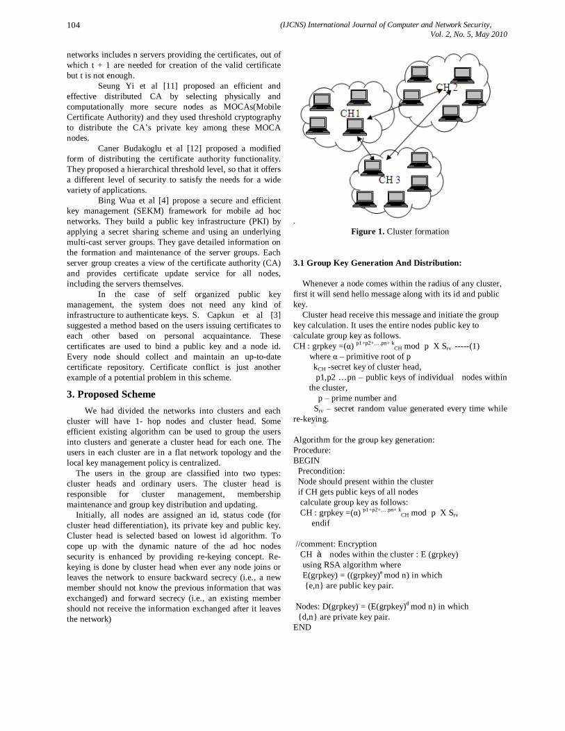
(IJCNS) International Journal of Computer and Network Security, Vol. 2, No. 5, May 2010
104
networks includes n servers providing the certificates, out of which t + 1 are needed for creation of the valid certificate but t is not enough.
Seung Yi et al [11] proposed an efficient and effective distributed CA by selecting physically and computationally more secure nodes as MOCAs(Mobile Certificate Authority) and they used threshold cryptography to distribute the CA’s private key among these MOCA nodes.
Caner Budakoglu et al [12] proposed a modified form of distributing the certificate authority functionality. They proposed a hierarchical threshold level, so that it offers a different level of security to satisfy the needs for a wide variety of applications.
Bing Wua et al [4] propose a secure and efficient key management (SEKM) framework for mobile ad hoc networks. They build a public key infrastructure (PKI) by applying a secret sharing scheme and using an underlying multi-cast server groups. They gave detailed information on the formation and maintenance of the server groups. Each server group creates a view of the certificate authority (CA) and provides certificate update service for all nodes, including the servers themselves.
In the case of self organized public key management, the system does not need any kind of infrastructure to authenticate keys. S. Capkun et al [3] suggested a method based on the users issuing certificates to each other based on personal acquaintance. These certificates are used to bind a public key and a node id. Every node should collect and maintain an up-to-date certificate repository. Certificate conflict is just another example of a potential problem in this scheme.
3. Proposed Scheme We had divided the networks into clusters and each cluster will have 1- hop nodes and cluster head. Some efficient existing algorithm can be used to group the users into clusters and generate a cluster head for each one. The users in each cluster are in a flat network topology and the local key management policy is centralized. The users in the group are classified into two types: cluster heads and ordinary users. The cluster head is responsible for cluster management, membership maintenance and group key distribution and updating. Initially, all nodes are assigned an id, status code (for cluster head differentiation), its private key and public key. Cluster head is selected based on lowest id algorithm. To cope up with the dynamic nature of the ad hoc nodes security is enhanced by providing re-keying concept. Re-keying is done by cluster head when ever any node joins or leaves the network to ensure backward secrecy (i.e., a new member should not know the previous information that was exchanged) and forward secrecy (i.e., an existing member should not receive the information exchanged after it leaves the network)
. Figure 1. Cluster formation
3.1 Group Key Generation And Distribution: Whenever a node comes within the radius of any cluster, first it will send hello message along with its id and public key. Cluster head receive this message and initiate the group key calculation. It uses the entire nodes public key to calculate group key as follows. CH : grpkey =(α) p1+p2+….pn+ k
CH mod p X Srv -----(1) where α – primitive root of p
kCH -secret key of cluster head, p1,p2 …pn – public keys of individual nodes within the cluster, p – prime number and
Srv – secret random value generated every time while re-keying. Algorithm for the group key generation: Procedure: BEGIN Precondition: Node should present within the cluster if CH gets public keys of all nodes calculate group key as follows: CH : grpkey =(α) p1+p2+….pn+ k
CH mod p X Srv endif //comment: Encryption CH à nodes within the cluster : E (grpkey) using RSA algorithm where E(grpkey) = ((grpkey)e mod n) in which e,n are public key pair. Nodes: D(grpkey) = (E(grpkey)d mod n) in which d,n are private key pair. END

(IJCNS) International Journal of Computer and Network Security, Vol. 2, No. 5, May 2010
105
The distribution of group key is done using RSA algorithm. Cluster head having (e,n) public key and every node maintains (d,n) private key. When ever any new node joins into the cluster, cluster head calculates new group key and multicast to already existing nodes. And cluster head unicast the group key to new node along with private key for RSA algorithm. 3.2 New Node Joins When ever a node A joins in the network the following messages are exchanged. Node A joins CH already existing nodes (hello msg, ida, pka,N) calculates new group key multicast group
key to all nodes unicast (grp key, private key(d,n)) First group key will be encrypted using RSA algorithm and it is again encrypted using new node public key. CH à new node: E(Pbnode , (E(e,[Ko]) || (d,n) ) ) where Pbnode - public key of new node, e, n - Public key pair of RSA algorithm and d, n - Private key pair of RSA algorithm. Initially the new node gets the RSA private key pair by decrypting received key information using its own private key, after then it decrypts using RSA private key to get group key. All other already existing nodes receive encrypted information and decrypt using RSA algorithm to get the updated group key. 3.3 Existing Node Leaves Whenever an existing node B leaves the cluster the following messages are exchanged. Node B leaves CH already existing nodes (leave msg, idb) calculates new group key unicast group key to all individual nodes (grp key, private key(d,n)) The group key is encrypted first using RSA algorithm and then using individual nodes public keys.
C = (M)e mod n (e,n) – public key ---(2)
M = (C)d mod n (d,n) – private key ---(3) Suppose if any node leaves the cluster to maintain forward secrecy, cluster head calculate new group key and also it will change key encryption key also. And using individual node’s public key, key encryption key will be transmitted and using that key group key will be encrypted. Cluster head will unicast this information to all the nodes.
CH à all node: E(Pbnode , (E(e,[Ko]) || (d,n) ) ) where Pbnode - public key of new node, e, n - Public key pair of RSA algorithm and d, n - Private key pair of RSA algorithm.
3.4 Providing Authentication Within the network, if any two nodes A and B want to communicate first it will authenticate each other. The authentication steps are as follows.
1. Node A calculate hash value using its (id, public key, group key) and transmit the hash value, id and public key to node B 2. Node B receive hash value and also it calculate new
hash value from A’s id, public key and group key. 3. Node B will check the received values and
calculated value both are equal or not. 4. If the hashed values are equal, it identifies the peer
node as authenticated node. Algorithm for authentication: Procedure: BEGIN Precondition: The nodes must wish to communicate with each other. if get the peer nodes public key and ID. calculate the hash value and transmit to the peer one. A à B : hash (ida ,pka, group key) || ida ,pka peer node : calcuate the same hash value. endif if both hash values are same both are authenticated nodes endif END 3.5 To maintain network connectivity After clustering, the cluster head has to do more computation and so its energy may drain fast. To check this we can use periodic hello message. If the cluster head is not done any re-keying operation for the threshold time of 20 s, it has to broadcast hello message. This network maintenance can be done with the help of monitoring nodes. This node can be next highest resource available node after the cluster head. This node will maintain a timer, it will check for any communication from CH. If it does not receive any message (or) rekeying information, it will send hello message to CH
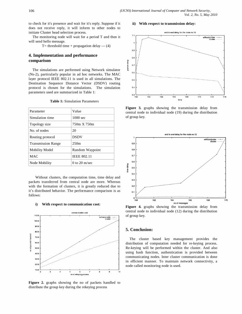
(IJCNS) International Journal of Computer and Network Security, Vol. 2, No. 5, May 2010
106
to check for it's presence and wait for it's reply. Suppose if it does not receive reply, it will inform to other nodes to initiate Cluster head selection process. The monitoring node will wait for a period T and then it will send hello message.
T= threshold time + propagation delay --- (4) 4. Implementation and performance comparison The simulations are performed using Network simulator (Ns-2), particularly popular in ad hoc networks. The MAC layer protocol IEEE 802.11 is used in all simulations. The Destination Sequence Distance Vector (DSDV) routing protocol is chosen for the simulations. The simulation parameters used are summarized in Table 1:
Table 1: Simulation Parameters Parameter Value
Simulation time 1000 sec
Topology size 750m X 750m
No. of nodes 20
Routing protocol DSDV
Transmission Range 250m
Mobility Model Random Waypoint
MAC IEEE 802.11
Node Mobility 0 to 20 m/sec
Without clusters, the computation time, time delay and packets transferred from central node are more. Whereas with the formation of clusters, it is greatly reduced due to it’s distributed behavior. The performance comparison is as follows:
i) With respect to communication cost:
Figure 2. graphs showing the no of packets handled to distribute the group key during the rekeying process
ii) With respect to transmission delay:
Figure 3. graphs showing the transmission delay from central node to individual node (19) during the distribution of group key.
Figure 4. graphs showing the transmission delay from central node to individual node (12) during the distribution of group key. 5. Conclusion: The cluster based key management provides the distribution of computation needed for re-keying process. Re-keying will be performed within the cluster. And also using hash function, authentication is provided between communicating nodes. Inter cluster communication is done in efficient manner. To maintain network connectivity, a node called monitoring node is used.

(IJCNS) International Journal of Computer and Network Security, Vol. 2, No. 5, May 2010
107
References [1] Aftab Ahmad, Mona El-Kadi Rizvi, Stephan Olariu
“Common Data Security Network (CDSN)” Q2SWinet’05, Montreal, Quebec, Canada, 2005.
[2] P.Papadimitratos and Z.J. Haas. "Secure Data Communication in Mobile Ad Hoc Networks" IEEE Journal on Selected Areas in Communications (JSAC), Special Issue on Security in Wireless Ad Hoc Networks, 2nd Quarter of 2006.
[3] S.Capkun, L. Butty´an, and J.-P. Hubaux. “Self-organized public-key management for mobile ad hoc networks” IEEE Transactions on MobileComputing, 2(1), January-March 2003.
[4] Bing Wu, Jie Wu, Eduardo B. Fernandez, Spyros Magliveras. “Secure and Efficient Key Management in Mobile Ad Hoc Networks” Proceedings of the 19th IEEE International Parallel and Distributed Processing Symposium (IPDPS’05) IEEE, 2005
[5] Ozkan M.Erdem.” Efficient Distributed Key Management for Mobile Ad Hoc Networks”0-7803-8623-W04, IEEE, 2004
[6] YANG Ya-tao, ZENG Ping, FANG Yong, CHI Ya-Ping. “A Feasible Key Management Scheme in Adhoc Network” Eighth ACIS International Conference on Software Engineering, Artificial Intelligence, Networking, and Parallel/Distributed, IEEE, 2007
[7] Zhou, L. and Z. Haas. “Securing Ad Hoc Networks”, IEEE Network Magazine, Vol. 13, 1999.
[8] Aldar C-F. Chan, “Distributed Symmetric Key Management for Mobile Ad hoc Networks”, IEEE INFOCOM, 2004.
[9] Atef Z. Ghalwash, Aliaa A. A. Youssif, Sherif M. Hashad and †Robin Doss “Self Adjusted Security Architecture for Mobile Ad Hoc Networks (MANETs)” 6th IEEE/ACIS International Conference on Computer and Information Science (ICIS 2007)
[10] Yanchao Zhang, Wei Liu, Wenjing Lou, and Yuguang Fang, “Securing Mobile Ad Hoc Networks with Certificateless Public Keys”, IEEE Transactions on Dependable and Secure Computing, vol. 3, No. 4, Oct-Dec 2006.
[11] Seung Yi, Robin Kravets, “Key Management for Heterogeneous Ad Hoc Wireless Networks ”, Proc. of the 10th IEEE International conference on Network Protocols (ICNP’02), pages 202-203, Nov. 2002.
[12] Caner Budakoglu and T.Aaron Gulliver, “Hierarchical Key Management for Mobile Ad Hoc Networks”, 0 -7803-8521-7/04 IEEE, 2004.
[13]Renuka. A and Shet K.C, “Cluster Based Group Key Management in Mobile Ad hoc Networks”, International Journal of Computer Science and Network Security, Vol 9, No 4, 2009.
[14] Patrick P.C.Lee, John C.S Lui, and David K.Y. Yau, “Distributed Collaborative Key Agreement and Authentication Protocols for Dynamic Peer Groups”, IEEE/ACM Transactions on Networking (TON) Volume 14, Issue 2 Pages: 263 – 276, 2006.
[15]Lihao Xu, and Cheng Huang, “Computation Efficient Multicast Key Distribution”, Parallel and Distributed
Systems, IEEE Transactions on Volume 19, Issue 5, Page(s):577 – 587, 2008.
[16]Kejie Lu, Yi Qian, Mohsen Guizani, and Hsiao-Hwa Chen, “A Framework for a Distributed Key Management Scheme in Heterogeneous Wireless Sensor Networks”, IEEE Transactions on Wireless Communications, Vol 7, No. 2, Feb’ 2008
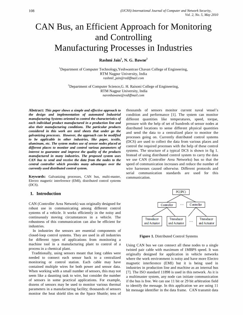
(IJCNS) International Journal of Computer and Network Security, Vol. 2, No. 5, May 2010
108
CAN Bus, an Efficient Approach for Monitoring and Controlling
Manufacturing Processes in Industries
Rashmi Jain1, N. G. Bawne2
1Department of Computer Technology,Yeshwantrao Chavan College of Engineering, RTM Nagpur University, India
2Department of Computer Science,G. H. Raisoni College of Engineering, RTM Nagpur University, India
Abstract: This paper shows a simple and effective approach to the design and implementation of automated Industrial manufacturing Systems oriented to control the characteristics of each individual product manufactured in a production line and also their manufacturing conditions. The particular products considered in this work are steel sheets that under go the galvanizing processes. However, the approach can be modified to be applicable in other industries, like paper, textile, aluminum, etc. The system makes use of sensor nodes placed at different places to monitor and control various parameters of interest to guarantee and improve the quality of the products manufactured in many industries. The proposed system uses CAN bus to send and receive the data from the nodes to the central controller which provides many advantages over the currently used distributed control system. Keywords: Galvanizing processes, CAN bus, multi-master, Electro magnetic interference (EMI), distributed control systems (DCS). 1. Introduction
CAN (Controller Area Network) was originally designed for robust use in communicating among different control systems of a vehicle. It works efficiently in the noisy and continuously moving circumstances in a vehicle. The robustness of this communication can also be efficient for industries. In industries the sensors are essential components of closed-loop control systems. They are used in all industries for different types of applications from monitoring a machine tool in a manufacturing plant to control of a process in a chemical plant. Traditionally, using sensors meant that long cables were needed to connect each sensor back to a centralized monitoring or control station. Each cable may have contained multiple wires for both power and sensor data. When working with a small number of sensors, this may not seem like a daunting task to wire, but consider the number of sensors in some practical applications. For example, dozens of sensors may be used to monitor various thermal parameters in a manufacturing facility; thousands of sensors monitor the heat shield tiles on the Space Shuttle; tens of
thousands of sensors monitor current naval vessel’s condition and performance [1]. The system can monitor different quantities like temperatures, speed, torque, pressure with the help of set of hundreds of sensor nodes at distributed locations to sense different physical quantities and send the data to a centralized place to monitor the processes going on. Currently distributed control systems (DCS) are used to collect the data from various places and control the required processes with the help of these control systems. The structure of a typical DCS is shown in fig 1. Instead of using distributed control system to carry the data we use CAN (Controller Area Networks) bus so that the speed of communication increases and reduce the number of wire harnesses caused otherwise. Different protocols and serial communication standards are used for this communication.
Figure 1. Distributed Control Systems
Using CAN bus we can connect all these nodes to a single twisted pair cable with maximum of 1MBPS speed. It was originally designed for application in vehicle networks where the work environment is noisy and have more Electro magnetic interference (EMI) but it is being used in industries in production line and machine as an internal bus [7]. The ISO standard 11898 is used in this network. As it is a multimaster system, any node can initiate communication if the bus is free. We can use 11 bit or 29 bit arbitration field to identify the message. In this application we are using 11 bit message identifier in the data frame. CAN transmit data
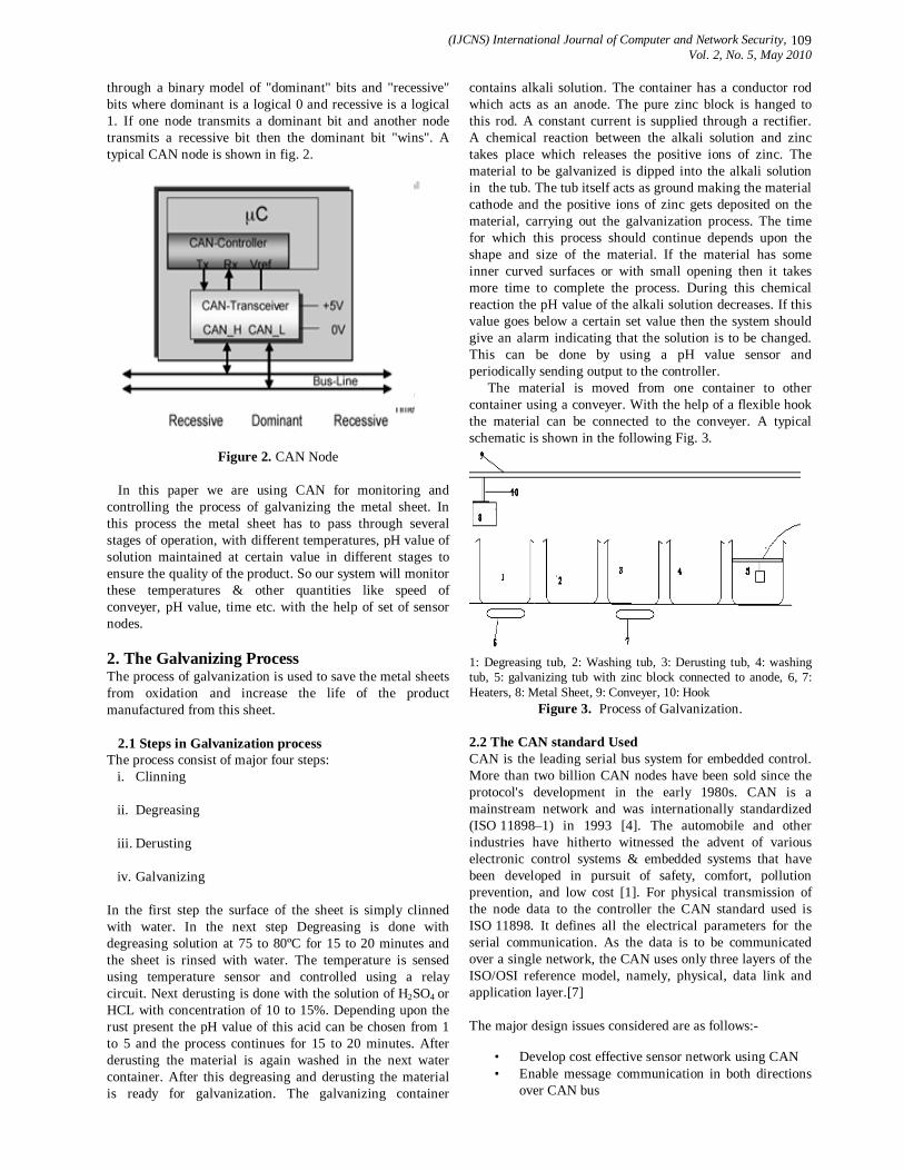
(IJCNS) International Journal of Computer and Network Security, Vol. 2, No. 5, May 2010
109
through a binary model of "dominant" bits and "recessive" bits where dominant is a logical 0 and recessive is a logical 1. If one node transmits a dominant bit and another node transmits a recessive bit then the dominant bit "wins". A typical CAN node is shown in fig. 2.
Figure 2. CAN Node
In this paper we are using CAN for monitoring and controlling the process of galvanizing the metal sheet. In this process the metal sheet has to pass through several stages of operation, with different temperatures, pH value of solution maintained at certain value in different stages to ensure the quality of the product. So our system will monitor these temperatures & other quantities like speed of conveyer, pH value, time etc. with the help of set of sensor nodes. 2. The Galvanizing Process The process of galvanization is used to save the metal sheets from oxidation and increase the life of the product manufactured from this sheet. 2.1 Steps in Galvanization process The process consist of major four steps:
i. Clinning
ii. Degreasing
iii. Derusting
iv. Galvanizing
In the first step the surface of the sheet is simply clinned with water. In the next step Degreasing is done with degreasing solution at 75 to 80ºC for 15 to 20 minutes and the sheet is rinsed with water. The temperature is sensed using temperature sensor and controlled using a relay circuit. Next derusting is done with the solution of H2SO4 or HCL with concentration of 10 to 15%. Depending upon the rust present the pH value of this acid can be chosen from 1 to 5 and the process continues for 15 to 20 minutes. After derusting the material is again washed in the next water container. After this degreasing and derusting the material is ready for galvanization. The galvanizing container
contains alkali solution. The container has a conductor rod which acts as an anode. The pure zinc block is hanged to this rod. A constant current is supplied through a rectifier. A chemical reaction between the alkali solution and zinc takes place which releases the positive ions of zinc. The material to be galvanized is dipped into the alkali solution in the tub. The tub itself acts as ground making the material cathode and the positive ions of zinc gets deposited on the material, carrying out the galvanization process. The time for which this process should continue depends upon the shape and size of the material. If the material has some inner curved surfaces or with small opening then it takes more time to complete the process. During this chemical reaction the pH value of the alkali solution decreases. If this value goes below a certain set value then the system should give an alarm indicating that the solution is to be changed. This can be done by using a pH value sensor and periodically sending output to the controller. The material is moved from one container to other container using a conveyer. With the help of a flexible hook the material can be connected to the conveyer. A typical schematic is shown in the following Fig. 3.
1: Degreasing tub, 2: Washing tub, 3: Derusting tub, 4: washing tub, 5: galvanizing tub with zinc block connected to anode, 6, 7: Heaters, 8: Metal Sheet, 9: Conveyer, 10: Hook
Figure 3. Process of Galvanization. 2.2 The CAN standard Used CAN is the leading serial bus system for embedded control. More than two billion CAN nodes have been sold since the protocol's development in the early 1980s. CAN is a mainstream network and was internationally standardized (ISO 11898–1) in 1993 [4]. The automobile and other industries have hitherto witnessed the advent of various electronic control systems & embedded systems that have been developed in pursuit of safety, comfort, pollution prevention, and low cost [1]. For physical transmission of the node data to the controller the CAN standard used is ISO 11898. It defines all the electrical parameters for the serial communication. As the data is to be communicated over a single network, the CAN uses only three layers of the ISO/OSI reference model, namely, physical, data link and application layer.[7] The major design issues considered are as follows:-
• Develop cost effective sensor network using CAN • Enable message communication in both directions
over CAN bus

(IJCNS) International Journal of Computer and Network Security, Vol. 2, No. 5, May 2010
110
• Flexibility in increasing number of nodes without any problem,
• Make system more reliable, as wire harnesses is reduced
3. The System Architecture
Various nodes with multiple sensors can be deployed in various sections to sense the quantity of interest and send it over the CAN bus to the base station as given in the block diagram in fig 5. Some processing is done on this data so that the size of the data to be further communicated to the server can be reduced and bandwidth utilization will be done efficiently. At the server end the data gathered will be analyzed for proper monitoring purpose and taking appropriate actions during the manufacturing process. The structure of the Centralized monitoring server is given in
following fig 4.
Figure 4. Centralized Monitoring Server
Figure 5. Node Structure Different nodes can have the number of sensors attached to them. Here for demonstration purpose we are using temperature senor, LM35, at a node. The data from the sensors is collected and processed by the microcontroller. The microcontroller used here is AVR ATMEGA16 which has an inbuilt 8 channel ADC implemented at port PA. The output of the temperature controller is given to PA0 pin. Microcontroller converts this to digital value and compares
it with the preset value. If the temperature is less than this set point then the heater is switched on with the help of a relay, otherwise it is switched off. This relay operates with he interrupt signal at pin PD3/INT1. The information generated i.e. current temperature value and status of relay, by the microcontroller is sent to the centralized controller through the CAN port for further processing. The CAN controller used is 8 pin chip MCP2551. It is connected to microcontroller at pins PD0/RXD and PD1/TXD. The circuit diagram of the node structure or slave unit is shown in fig. 6.
GND
12V VCC
12V
PA0/ADC040
PA1/ADC139
PA2/ADC238
PA3/ADC337
PA4/ADC436
PA5/ADC535
PA6/ADC634
PB0/XCK/T01
PB1/T12
PB2/INT2/AIN03
PB3/OC0/AIN14
PB4/SS5
PB5/MOSI6
PB6/MISO7
PB7/SCK8
PA7/ADC733
RESET9
XTAL113
XTAL212
PC0/SCL 22
PC1/SDA 23
PC2/TCK 24
PC3/TMS 25
PC4/TDO 26
PC5/TDI 27
PC6/TOSC1 28
PC7/TOSC2 29
PD0/RXD 14
PD1/TXD 15
PD2/INT0 16
PD3/INT1 17
PD4/OC1B 18
PD5/OC1A 19
PD6/ICP 20
PD7/OC2 21
AVCC 30
AREF 32
U1
ATMEGA16
A8 R 2
Y5
D 3
B7
Z6
U2
MCP2551
162738495
J2
CONN-D9M
CAN BUS
R1
47k
D1
1N4007D2
1N4007
C12200u
VI1 VO 3
GN
D2
U47805
C2100n
C3100n
123
J3
CONN-SIL3
SLAVE UNIT
POWER SUPPLY
GN
D3
+VS
1
VOUT 2
U3
LM35
TEMP SENSOR
RL1OMI-SH-124L
Q1BC547
R247k
OUTPUT RELAY
Figure 6. Circuit Diagram of Node Centralized controller may use some keypad with 3 buttons UP, DOWN, ENTER for entering the new set points by increasing or decreasing the current set point. A LCD (16 X 2 lines) is used to display value of temperature and the status of the relay. To receive the information from the nodes and sending new set point it again uses the CAN port. ATMEGA16 is used as the controller here. For further use and storage of the monitored data it is sent to the PC via serial communication port, MAX232 [7]. It is connected to the TXD and RXD pins of the microcontroller. The circuit diagram of the Centralized controller is shown in fig. 7. Both the circuits use the regulated power supply which will give 5V output for driving the circuits.
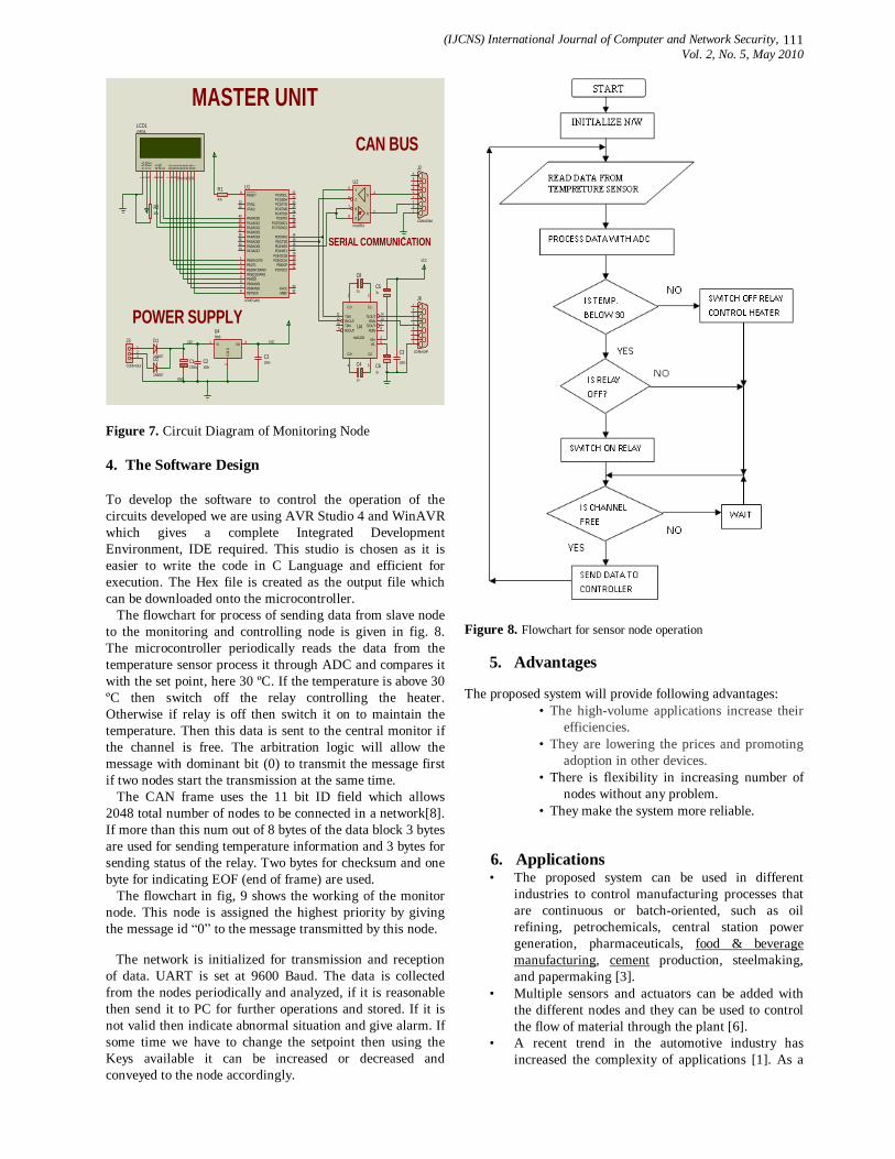
(IJCNS) International Journal of Computer and Network Security, Vol. 2, No. 5, May 2010
111
GND
12V VCC
PA0/ADC040
PA1/ADC139
PA2/ADC238
PA3/ADC337
PA4/ADC436
PA5/ADC535
PA6/ADC634
PB0/XCK/T01
PB1/T12
PB2/INT2/AIN03
PB3/OC0/AIN14
PB4/SS5
PB5/MOSI6
PB6/MISO7
PB7/SCK8
PA7/ADC733
RESET9
XTAL113
XTAL212
PC0/SCL 22
PC1/SDA 23
PC2/TCK 24
PC3/TMS 25
PC4/TDO 26
PC5/TDI 27
PC6/TOSC1 28
PC7/TOSC2 29
PD0/RXD 14
PD1/TXD 15
PD2/INT0 16
PD3/INT1 17
PD4/OC1B 18
PD5/OC1A 19
PD6/ICP 20
PD7/OC2 21
AVCC 30
AREF 32
U1
ATMEGA16
A8 R 2
Y5
D 3
B7
Z6
U2
mcp2551
D7
14D
613
D5
12D
411
D3
10D
29
D1
8D
07
E6
RW5
RS
4
VSS
1V
DD
2V
EE3
LCD1LM016L
162738495
J2
CONN-D9M
C4
1u
C51u
C61u
C8
1u
T1IN11
R1OUT12
T2IN10
R2OUT9
T1OUT 14
R1IN 13
T2OUT 7
R2IN 8
C2+
4
C2-
5
C1+
1
C1-
3
VS+ 2
VS- 6
U4
MAX232
162738495
J6
CONN-D9F
VCC
C3
100n
SERIAL COMMUNICATION
CAN BUS
R1
47k
R247k
D1
1N4007D2
1N4007
C12200u
VI1 VO 3
GN
D2
U47805
C2100n
C3100n
123
J3
CONN-SIL3
MASTER UNIT
POWER SUPPLY
Figure 7. Circuit Diagram of Monitoring Node 4. The Software Design To develop the software to control the operation of the circuits developed we are using AVR Studio 4 and WinAVR which gives a complete Integrated Development Environment, IDE required. This studio is chosen as it is easier to write the code in C Language and efficient for execution. The Hex file is created as the output file which can be downloaded onto the microcontroller. The flowchart for process of sending data from slave node to the monitoring and controlling node is given in fig. 8. The microcontroller periodically reads the data from the temperature sensor process it through ADC and compares it with the set point, here 30 ºC. If the temperature is above 30 ºC then switch off the relay controlling the heater. Otherwise if relay is off then switch it on to maintain the temperature. Then this data is sent to the central monitor if the channel is free. The arbitration logic will allow the message with dominant bit (0) to transmit the message first if two nodes start the transmission at the same time. The CAN frame uses the 11 bit ID field which allows 2048 total number of nodes to be connected in a network[8]. If more than this num out of 8 bytes of the data block 3 bytes are used for sending temperature information and 3 bytes for sending status of the relay. Two bytes for checksum and one byte for indicating EOF (end of frame) are used. The flowchart in fig, 9 shows the working of the monitor node. This node is assigned the highest priority by giving the message id “0” to the message transmitted by this node.
The network is initialized for transmission and reception of data. UART is set at 9600 Baud. The data is collected from the nodes periodically and analyzed, if it is reasonable then send it to PC for further operations and stored. If it is not valid then indicate abnormal situation and give alarm. If some time we have to change the setpoint then using the Keys available it can be increased or decreased and conveyed to the node accordingly.
Figure 8. Flowchart for sensor node operation
5. Advantages
The proposed system will provide following advantages: • The high-volume applications increase their
efficiencies. • They are lowering the prices and promoting
adoption in other devices. • There is flexibility in increasing number of
nodes without any problem. • They make the system more reliable.
6. Applications • The proposed system can be used in different
industries to control manufacturing processes that are continuous or batch-oriented, such as oil refining, petrochemicals, central station power generation, pharmaceuticals, food & beverage manufacturing, cement production, steelmaking, and papermaking [3].
• Multiple sensors and actuators can be added with the different nodes and they can be used to control the flow of material through the plant [6].
• A recent trend in the automotive industry has increased the complexity of applications [1]. As a

(IJCNS) International Journal of Computer and Network Security, Vol. 2, No. 5, May 2010
112
result, the number of nodes connected to the CAN bus has increased.
• Safety and efficiency requirements such as latency, high data rate, immunity to noise, and error-detection capability are challenging the current CAN capabilities.
Figure 9. Flowchart for Controller node operation
7. Conclusion
The system developed with the help of sensor nodes and CAN Bus improves the performance of the system and reliability of the system at lower costs as compared to the presently applied system of distributed control systems using RS-232 based communication. Multimaster communication allows any node to initiate communication when bus is free. The intelligent nodes make proper utilization of the bus. Automobile industries and other industries are making use of it for better noise immunity and EMI. Along with the application in vehicle networks CAN bus is efficiently used in industries also. In the Galvanization process also the quality of the finished product will increase if all the phases are completed in due course of stipulated time and at controlled temperature and pH value of the solution. References [1] W. Xing, H. Chen, H. Ding, “The Application of
Controller Area Network on Vehicle”, Proc. IVEC, 1999, pp. 455 – 458.
[2] Krishna Chaitanya Emani, Keong Kam, Maciej
Zawodniok Yahong Rosa Zheng, Jagannathan Sarangapani, “Improvement of CAN Bus Performance By Using Error-Correction Codes”, IEEE Region 5 Technical, Professional & Student conference 2007.
[3] Ian F. Akyildiz, Weilian Su, Yogesh Sankarasubramaniam,“A Survey on Sensor Networks”, Erdal Cayirci Georgia Instetude of Technology. IEEE Communication Magazine- August 2002
[4] Kay R¨omer and Friedemann Mattern, “The Design Space of Wireless Sensor Networks”, IEEE Wireless Communications, Dec. 2004.
[5] Ping Ran, Baoqiang Wang, Wei Wang, “The Design of Communication Convertor Based on CAN Bus”, Proceedings of the 2008 IEEE/ASME International Conference on Advanced Intelligent Mechatronics, July 2 - 5, 2008.
[6] William Kaisar and Gregory Pottie, “Principles of
Embedded Network System Design”, First edition, Cambridge University Press 2005.
[7] Xia Dong, Kedian Wang, Kai Zhao, “Design and Implementation of an Automatic Weighing System Based on CAN Bus”,,Proceedings of the 2008 IEEE/ASME International Conference on Advanced Intelligent Mechatronics July 2 - 5, 2008...O
[8] Javier Diaz, Elias Rodriguez, Luis Hurtado, Hugo
Cacique, Nimrod Vazquez, Agustin Ramirez,,“CAN Bus Embedded System for Lighting Network Applications Proceedings of the 2008 IEEE/ASME International Conference on Advanced Intelligent Mechatronics, July 2 - 5, 2008.
Authors Profile
Rashmi Jain completed her B. E. (Computer Technology) from Kavi Kulguru Institute of Technology and Science, Nagpur University in 1997. Currently completing M.E. in Embedded systems and Computing from G. H. Raisoni College of Engineering, Nagpur University. Meanwhile worked as a lecturer in Comp. Tech. Dept. at KITS Ramtek, SSGMCE Shegaon and YCCE Nagpur.ET VOLUME 31
JULY 2008 ISSN 1307-6884 513 © 2008 WASET.ORG Dr. Narendra G Bawane is Professor and Former Head of Computer Science and Engineering department at G. H. Raisoni college of Engineering, Nagpur (Maharashtra). Prior to this assignment, he worked with B.D. College of Engineering Sewagram and Govt. Polytechnic, Nagpur for several years. He has total teaching experience of more than 22 years. He has
completed his B.E. from Nagpur University in 1987 and M. Tech. in 1992 from IIT, New Delhi. He completed his Ph. D. in 2006 at VNIT, Nagpur.
(IJCNS) International Journal of Computer and Network Security, Vol. 2, No. 5, May 2010
113
A Novel Architecture for QoS Management in MANET using Mobile Agent
A.K.Vatsa1 and Gaurav Kumar2
1Assistant Professor
School of Computer Engineering and Information Technology, SHOBHIT UNIVERSITY, NH-58, MODIPURAM, MEERUT, UTTAR PRADESH, INDIA.
2Bachelor of Technology School of Computer Engineering and Information Technology, SHOBHIT UNIVERSITY,
NH-58, MODIPURAM, MEERUT, UTTAR PRADESH, INDIA. [email protected]
Abstract: The wide availability of mobile devices equipped with infrastructure-free wireless communication capabilities together with the technical possibility to form ad-hoc networks paved the path for building highly dynamic communities of mobile users. In many performance oriented applications like co-operative information sharing, defense applications, disaster management, mission critical applications and commercial production applications needs QoS, which is, no doubt, a critical issue. In this paper, we propose a novel architecture using hierarchical model to effectively manage the resources on and attached with Mobile ad-hoc Network and provide robustness with zero probability of fault. The dynamic clustering and the criteria for cluster formation causes adaptability to various situations and enhancement of load bearing capacity as well as an effective co-operation between several nodes to bear the responsibilities. The main focus is to minimize the overhead transmission in the network for which a new approach of co-operative routing is implemented.
Keywords: MANET, QoS, Mobile Agent, Cluster, Cluster Head, co-operative Routing, Hierarchical model, Dynamic Clustering, Hybrid Approach and Host.
1. Introduction 1.1 MANET
Mobile Ad hoc network [9], is infrastructure less, dynamic multi-hop wireless network, where each node acts as a mobile router. They are equipped with a wireless transceiver and by a group of mobile hosts formed on a shared wireless channel by virtue of their proximity to each other [10]. Routing protocols should adapt to such dynamics and continue to maintain connection between the communicating nodes. As a consequence of mobility and disconnection of mobile hosts, the dynamics of wireless ad hoc networks, causes a lot of problems to emerge in designing proper routing algorithms for effective communication [11]-[12]. Also the time of entering the node to the network and exiting from it be unpredictable. Work on unipath routing has been proposed in many literatures [18]-[22]. There two main classes of routing protocols in MANET, i.e., table-based or proactive and on demand or reactive protocols [23]. Any suitable mix may give better results. Their varied scope and promising features cause
interest in this field and researches to be carried out for betterment of the network functioning.
1.2 Mobile Agent Mobile agents are programs that can migrate from host to host in a network [11], at times and to places of their own choosing where this is mandatory for the host to posses’ agent hosting capability. The agent code should not have to be installed on every machine the agent could visit providing them platform independency [11]. Agents are able to decide, based on their local knowledge, if, when and where to migrate in the network. The ability of mobile agents to replicate themselves into many copies that travel to different points across the network sounds promising. During migration, the agent’s local state variables [7] are transferred to the new host to continue computation there. Mobile agents are chosen for many applications, due to several reasons [8], viz. improvements in latency and bandwidth of client-server applications and reducing vulnerability to network disconnection.
1.3 Quality of Service QoS support in MANET’s is a challenging task and it is required to have a better management over parameters like minimum bandwidth; minimum delay, jitter guarantee, dis-connectivity and denial of services and contract based enforced service agreements. Although, MANET’s are used for a variety of applications, but, the commercial one’s mainly multimedia applications require a predefined Quality of Service [1]. This QoS is in the form of an agreed upon service level agreement [1]. QoS means a guarantee of some parameters and their threshold value. We know that different applications have different requirements of resources. QoS roughly means providing the applications with enough network resources, so that they can function within acceptable performance limits. Since the requirements of resources vary, the value of QoS parameters also varies for every application.
1.4 Problem Identification The problem considered in this paper is to provide a routing scheme for MANET’s so that the QoS can be provided to the mobile nodes with decreasing the amount of overhead transmission and providing such an architecture which
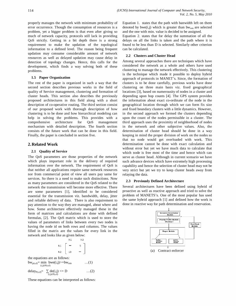
(IJCNS) International Journal of Computer and Network Security, Vol. 2, No. 5, May 2010
114
properly manages the network with minimum probability of error occurrence. Though the consumption of resources is a problem, yet a bigger problem is that even after giving so much of network capacity, protocols still lack in providing QoS strictly. Getting in a bit depth there is a strong requirement to make the updation of the topological information to a defined level. The reason being frequent updation may consume considerable amount of network resources as well as delayed updation may cause delay in detection of topology changes. Hence, this calls for the development, which finds a way solving both of these problems.
1.5 Paper Organization The rest of the paper is organized in such a way that the second section describes previous works in the field of quality of Service management, clustering and formation of cluster heads. This section also describes the previously proposed architectures in this field along with a short description of co-operative routing. The third section consist of our proposed work with thorough description of how clustering is to be done and how hierarchical modeling can help in solving the problems. This provides with a comprehensive architecture for QoS management mechanism with detailed description. The fourth section consists of the future work that can be done in this field. Finally, the paper is concluded in section five.
2. Related Work 2.1 Quality of Service
The QoS parameters are those properties of the network which plays important role in the delivery of required information over the network. The requirement of QoS is that neither all applications require same network resources nor from commercial point of view all users pay same for services. So there is a need to make such distinctions. Now as many parameters are considered in the QoS related to the network the transmission will become more effective. There are some parameters [1], identified to be considered essential for the transmission viz. bandwidth, delay, jitter and reliable delivery of data. There is also requirement to pay attention to the way they are managed, about where and how. Some architecture effectively managed these in the form of matrices and calculations are done with defined formulas, [2]. The QoS matrix which is used to store the values of parameters of links between every two nodes is having the node id on both rows and columns. The values filled in the matrix are the values for every link in the network and looks like as given below:
the equations are as follows: bwp(s,d)= min bwe(i,j)>=bwmin …(1) (i,j)έP(s,d)
delayP(s,d)= ∑ de(i,j) <= D …(2) (i,j)έP(s,d)
These equations can be interpreted as follows:
Equation 1. states that the path with banwidth left on them denoted by bwe(i,j) which is greater than bwmin are selected and the one with min. value is decided to be assigned. Equation 2. states that for delay the summation of all the delays on all the links is taken and the path where it is found to be less than D is selected. Similarly other criterion can be calculated.
2.2 Clusters and Cluster Head Among several approaches there are techniques which have considered the network as a whole and others have used clustering to manage the network effectively. This clustering is the technique which made it possible to deploy hybrid approach of protocols in MANET’s. Since, the formation of clusters is to be done carefully, previous works have done clustering on three main basis viz. fixed geographical locations [3], based on numerousity of nodes in a cluster and depending upon hop counts [4]. The GPS system provides the information about exact co-ordinate of the node in the geographical location through which we can form fix size and fixed boundary clusters with a little dynamics. However, in the second approach we formed the clusters depending upon the count of the nodes permissible in a cluster. The third approach uses the proximity of neighborhood of nodes in the network and other subjective values. Also, the determination of cluster head should be done in a way keeping in mind the proper division of work on the nodes so that no node would get overloaded with work. This determination cannot be done with exact calculation and without error but yet we have much data to calculate that which node is free most of the time and hence which can serve as cluster head. Although in current scenario we have such advance devices which have extremely high processing capability and hence the selection of cluster head may not be very strict but yet we try to keep cluster heads away from relaying the data.
2.3 Previously Defined Architecture Several architectures have been defined using hybrid of proactive as well as reactive approach and tried to solve the problem of MANETS’s. One of the most popular has used the same hybrid approach [1] and defined how the work is done in reactive way for path determination and reservation.
(a) Contract enforcer
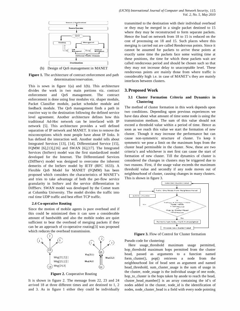
(IJCNS) International Journal of Computer and Network Security, Vol. 2, No. 5, May 2010
115
(b) Design of QoS management in MANET
Figure 1. The architecture of contract enforcement and path determination/reservation.
This is sown in figure 1(a) and 1(b). This architecture divides the work in two main portions viz. contract enforcement and QoS management. The contract enforcement is done using four modules viz. shaper module, Packet Classifier module, packet scheduler module and feedback module. The QoS management finds a path in reactive way to the destination following the defined service level agreement. Another architecture defines how this traditional Ad-Hoc network can be interfaced with IP network [5]. This architecture provides a well defined separation of IP network and MANET. It tries to remove the misconceptions which most people have about IP links. It has defined the interaction well. Another model tells about Integrated Services [13], [14], Differentiated Service [15], FQMM [6],[13],[16] and SWAN [6],[17]. The Integrated Services (IntServ) model was the first standardized model developed for the Internet. The Differentiated Services (DiffServ) model was designed to overcome the inherent demerits of the IntServ model by IETF (RFC 1633). A Flexible QoS Model for MANET (FQMM) has been proposed which considers the characteristics of MANET’s and tries to take advantage of both the per-flow service granularity in IntServ and the service differentiation in DiffServ. SWAN model was developed by the Comet team at Columbia University. The model divides the traffic into real time UDP traffic and best effort TCP traffic.
2.4 Co-operative Routing Since the motion of mobile agents is pure overhead and if this could be minimized then it can save a considerable amount of bandwidth and also the mobile nodes are quiet sufficient to bear the overhead of merging packets if they can be an approach of co-operative routing[3] was proposed which reduces the overhead transmission.
Figure 2. Cooperative Routing
It is shown in figure 2. The message from 22, 23 and 24 arrived 18 at three different times and are destined to 1, 2 and 3. As in figure 1 either they could be individually
transmitted to the destination with their individual overhead or they may be merged in a single packet destined to 15 where they may be reconstructed to form separate packets. Hence the load on network from 18 to 15 is reduced on the cost of processing on 18 and 15. Such places where this merging is carried out are called Rendezvous points. Since it cannot be assumed for packets to arrive these points at exactly same time the packets face some waiting time at these positions, the time for which these packets wait are called rendezvous period and should be chosen such so that they may not increase delay to unacceptable level. These rendezvous points are mainly those from where traffic is considerably high i.e. in case of MANET’s they are mainly interfaces between clusters.
3. Proposed Work 3.1 Cluster Formation Criteria and Dynamics in
Clustering The method of cluster formation in this work depends upon two conditions. Depending upon previous experiences we have data about what amount of time some node is using the transmission medium. The sum of this value should not exceed a threshold value within a period of time. Hence as soon as we reach this value we start the formation of new cluster. Though it may increase the performance but can cause non-symmetric structure of cluster. To keep it symmetric we pose a limit on the maximum hops from the cluster head permissible in the cluster. Now, these are two criteria’s and whichever is met first can cause the start of formation of new cluster. Till the dynamics of cluster is considered the changes in clusters may be triggered due to two reasons. First, if the usage value exceeds the maximum threshold value and secondly if any node moves out of neighbourhood of cluster, causing changes in many clusters. This is shown in figure 3.
Figure 3. Flow of Control for Cluster formation
Pseudo code for clustering: Here usage_threshold maximum usage permitted, hop_threshold maximum hops permitted from the cluster head, passed as arguments to a function named form_cluster(), pop() retrieves a node from the neighbourhood list of head sent as argument and named head_threshold, sum_cluster_usage is the sum of usage in the cluster, node_usage is the individual usage of one node, hop_to_cluster is the hops taken by anode to reach the head, cluster_head_mamber[] is an array containing the id’s of nodes added in the cluster, node_id is the identification of nodes, node_cluster_head is a field with every node pointing

(IJCNS) International Journal of Computer and Network Security, Vol. 2, No. 5, May 2010
116
to the cluster head of itself, current_cluster_head is the head of the cluster for which clustering is done presently and least_usage_value is a function finding the node with least usage among unassigned nodes kept in a list and passed as argument called list_unassigned_node.
form_cluster(usage_threshold,hop_threshold) (1) pop(head_neighbourhood) (2) if(sum_cluster_usage+node_usage <
usage_threshold || hop_to_cluster < hop_threshold) (3) then: cluster_head_member[next]= node_id; (4) :node_cluster_head= cluster_head_id; (5) else current_cluster_head =
least_usage_value(list_unassigned_node) (6) goto step(1);
3.3 Hierarchical Model The hierarchy in the network means dividing the network in smaller regions and managing the regions as if they are small MANET’s. This is like the divide and conquers approach in the algorithms which we use to divide the problem in smaller parts. Initially it looks like the same clustering approach. This gives us several benefits, as this may divide the load between several nodes to maintain the topology of the network. This hierarchy will also cause effective path determination as well as routing and need not to travel on any path which may not lead to the destination. This causes the QoS effectively managed. The hierarchy which we use is rooted to several levels and taking an abstract view the functioning is similar. The cluster formation criterions which are previously described can be used to make upper layer clusters. Now consider a tree where root is the complete MANET and the leaves are the lowest and most fundamental clusters. Each node on the n-1th level is a group of these fundamental clusters. All such clusters on every level are on equivalent positions on the network. The formation and splitting criteria are same except the values which will be different in every level. The values will also be dynamically generated since there is no limitation over maximum Value of levels. This can be better shown by figure below. The hierarchical model is maintained by a mobile agent instances of which are travelling in the network inside each cluster and instances are also running on every level in proactive way updating the information after every certain time intervals. Also this mobile agent waits for some time on every node. There are nodes which act as interfaces between clusters acting as Rendezvous points where mobile agents co-operate to carry the information. It is illustrated in figure 4.
Figure 4. Cluster Formation and Hierarchical Model
3.2 Architecture The architecture shown in the figure is just a more detailed and modified form a previously proposed architectures. This architecture mainly defines the way in which path determination is done in case of multilevel hierarchical model and reservation is done afterwards. The architecture can be referred in figure 5. This calls for generation of a mobile agent on demand hence reactive in nature. The agent after finding the QoS path to the destination returns via same path to the source reserving resources at each intermediate cluster head. If the reservation fails due to reservation of resources by some other agent meanwhile, then again the path determination is done. However the path determination phase requires contract as well as the information of network capacity left at that time which is maintained by the cluster heads.
Figure 5. The Proposed Architecture for QoS management
3.3 Working Principle and Explanation
3.3.1 Hybrid Approach The previously defined problem of finding a way between high bandwidth consumption for overhead transmission and delayed updation can be better solved by the hybrid approach where at each level the topological information is updated by mobile agent for every cluster after certain time and the path determination can be done in reactive way by another mobile agent on demand. Before coming on to the actual description of operation of mobile agents we must discuss that there are several instances of same mobile agent travelling in the network and hence to distinguish between them we need to give every instance a unique Id.
3.3.2 Topology Maintaining Mobile Agent The mode of operation can be described in following steps: • Every node performs the neighbouhood detection. Each
node must detect the neighbor nodes with which it has a direct link. Neighbor Discovery Protocol (NDP) is used to discover the neighbors and update the neighbors table. It periodically transmits HELLO message at regular intervals. The reception of NDP beacons indicates "node found" or "node unreachable" information, the node will respond as follows:
Node found NDP packet: upon receiving a beacon from a new neighbor; the neighbor table is updated by adding this neighbor information as a new record with a zero in the NV field. Unreachable NDP packet: NDP packet could be detected as an unreachable neighbor node, so that neighbor record will be deleted from the neighbors table. • If any change is detected, it is communicated to mobile
agent when comes to the node. The motive of communicating only changes is to minimize the amount

(IJCNS) International Journal of Computer and Network Security, Vol. 2, No. 5, May 2010
117
of load on network again on the cost of extra processing on the side of nodes.
• This mobile agent moves inside the cluster and collects all such information as well as updates all such information on the node. This causes the maintenance of topology of the cluster on every node. The cluster head calculates some figures about the paths and the network capacity left with its cluster. This complete information with the agent is updated when it reaches the cluster head. It is later on communicated to the higher level cluster head by another agent and the process of updation goes on to maintain the complete topological information.
This updation in upper level cluster is done in following way: • The information of cluster available at lower level is
calculated to generate some information for upper layer cluster head.
• Every such lower level cluster head is travelled through interfaces by agent and agent for this level takes information from cluster heads only.
• This information is updated for upper level cluster head. An important point to be noted is that the generated information is not the info about each link but an abstract knowledge of the bandwidth available through that cluster, delay through that cluster and similar information about other parameters. Also if some change in the node membership is encountered. In this way the info is updated at the highest cluster head.
3.3.3 Path Determining and Resource Reserving Mobile Agent
The process of path determination and reservation is done by another mobile agent who works in the following way: • Whenever any node needs to transmit the data, it
generates the mobile agent and directs it to the cluster head.
• At cluster head if the destination node is in the current cluster then the head tells a QoS path to the agent.
• If the destination is not in the current cluster, the agent is told the way for upper layer cluster head.
• The process is repeated till the cluster of some level tells that the node is available in its cluster. From here the agent takes the path from source to destination following the lowest level clusters.
• This movement of the mobile agent till it reaches such a cluster head which has both the source and destination in its region causes the agent to see from the highest level the topology of the required region.
• The agent then reaches the destination’s lowest cluster head following the told path by the cluster head.
At this stage the path to the destination cluster is known. All the intermediate cluster heads of lowest level are then travelled in reverse order to reserve the path resources for the source in the following way: • The agent itself returns from the lowest level cluster
heads, intermediate in the path. • At every cluster head it reaches intermediately it reserves
the required amount of resources which should strictly follow the contract.
• The agent reaches back to the source. In this way a quality of service path is reserved for the source.
The last packet of transmission moves on with setting resources free. For this we need a special field value of which causes continuation of reservation or setting resources free.
3.3.4 QoS Path Determination in detail This process is done by reaching every cluster head and collecting the information for various parameters. The formulas in equation 1 and 2 are as it is followed in our work and give a clear picture about how the calculations are done to determine the paths fulfilling the criteria. However from the side of cluster head the responsibilities are to provide access to the data on the node about its cluster to the mobile agent. The rest is on the agent. Whenever the destination node is found in the cluster the head is responsible to tell the lowest level QoS path. In case of failure of path determination an alternative path is chosen, which in our work, we try to prepare for, if it happens to occur. For this we maintain several such paths and choose alternative on the spot. However, choosing such alternative path may constrain our future selections. If all such paths are not found then we move forward for second execution of path determination. Another point which should be considered is there are some QoS parameters which themselves depend upon other parameters such as delay or congestion, jitter and reliability on mobility of nodes etc. The guarantee for control of jitter is given by cashing of packets i.e. in case a data packet is delayed due to excessive traffic load or caused due to new path selection then the packet already cashed in the memory is used to make up the delivery gap. Another thing to be considered is the handoff process. If handoff occurs frequently, it has adverse effect on every aspect of QoS. Hence several factors which could cause potential problems during handoff are also managed under QoS. This management of QoS during handoff is considered differently. During handoff process, the data available at the cluster head is to be transmitted to the new cluster head. This transmission of data is always inter-cluster in cases when the handoff is due to head moving out of the cluster, since the indication of need of handoff is received only at the motion of head out of the cluster. Also the handoff may occur if the load on the node is so increased that it can no more bear the responsibility of cluster head in that case the handoff is intra-cluster. To manage this handoff process we divide the information available at the cluster head to be divided into two parts:
1) Readily available 2) Calculated information
This readily available information is the one which can be gathered inside the cluster as and when it is required. The calculated info is very concentrated and calculated from a long time in the past. Now since the handoff process requires some transfer of information about the cluster if the cluster head is leaving the cluster this transferred info would be only the calculated info. The will be gathered by a request.
(IJCNS) International Journal of Computer and Network Security, Vol. 2, No. 5, May 2010
118
4. Conclusion The architecture proposed and the model used solves the problem of management of topology and providing QoS in a better way than any other work proposed in this field however the practicality and implementation are no doubt matter of molding the proposals and to change them the way they fit. Higher load of processing is imposed on the nodes having ample amount of processing capacity and the load of transmission is reduced thereby saving bandwidth. Reliability of the routing protocol depends on its performance within highly dynamic networks. Scalability is determined by the protocol's performance at crowded networks. QoS is expressed by the protocol resistance to the network changes. Applying divide and conquer approach used in this design helps to effectively manage the network in highly dynamic situations and decreases the probability of fault on the network.
5. Future Scope The architecture in view of its functioning provides a strict set of rules for effective management of QoS in MANET’s yet it deserves thorough study and simulation on some test bed to evaluate its practical results and feasibility. Still the work can be done to minimize the overhead transmission for topology maintenance. If feasible to deploy in practical environment GPS tracking can also be used to reduce load on bandwidth. Also fixed geographical clustering has its own advantages and hence can be modified in similar way to reduce load. Consider agent's size, especially in scalable networks. Minimizing agent size may benefit from the idea of MPRs. Regulate TtM value depending on the network state to save the unnecessary fast updating. Adjust the agent population to maintain the optimal node-agent ratio in the network.
References [1] M.Sulleman Memon, Manzoor Hashmani and Niaz
A.Memon,A Framework for QoS Management and Contract Enforced Services in MANETs for Prioritized Traffic Environment, IJCSNS International Journal of Computer Science and Network Security, VOL.9 No.4, April 2009.
[2] S.S.Manvi and P.Venkataram, Mobile agent based approach for QoS routing, The Institution of Engineering and Technology 2007.
[3] Parama Bhaumik, Somprokash Banyopadhyay, Mobile Agent Based Message Communication in Large Ad hoc Networks through Co-operative Routing using Inter-Agent Negotiation at Rendezvous Points.
[4] S.A.Hosseini-Seno, B.Pahlevanzadeh, T.C.Wan, R. Budiarto, M.M.Kadhum, A DISTRIBUTED RESOURCE-MANAGEMENT APPROACH IN MANETS, Journal of Engineering Science and Technology Vol. 4, No. 2 (2009) 142 – 153,2009.
[5] Thomas Heide Clausen, A MANET Architecture Model, INSTITUT NATIONAL DE RECHERCHE EN INFORMATIQUE ET EN AUTOMATIQUE, January 2007.
[6] John B. Oladosu, Akinwale O. Alao, Matthew O. Adigun, Justice O. Emuoyibofarhe, Design and Simulation of a Quality of Service (QoS) Guaranteed Model for Mobile Ad Hoc Networks.
[7] David Kotz and Robert S. Gray, Mobile Agents and the Future of the Internet, ACM Operating Systems Review, August 1999, pp. 7-13
[8] Danny B. Lange and Mitsuru Oshima. Seven good reasons for mobile agents Communications of the ACM, 42(3):88– 89, March 1999.
[9] Corson, S., J.Macker, “Mobile ad hoc networking (MANET): routing protocol performance issues and evaluation considerations,” RFC 2501, Jan.1999.
[10] Hakim Badis and Khaldoun Al Agha, An Efficient QOLSR Extension Protocol For QoS in Ad hoc Networks.
[11] Manal Abdullah, Helen Bakhsh, Agent-based Dynamic Routing System for MANETs, ICGST-CNIR Journal, Volume 9, Issue 1, July 2009.
[12] K. A. H. Amin, “resource efficient and scalable routing using,” university of north texas, 2003.
[13] Hannan Xiao, Winston K.G. Seah, Anthony L O and Kee Chaing Chua, A flexible Quality of service Model For Mobile Ad-Hoc Networks, IEEE, 2000
[14] R. Braden, D. Clark, and S. Shenker, “Integrated Services in the Internet Architecture – an Overview,” IETF RFC1663, June 1994.
[15] K. Nichols, V. Jacobson, and L. Zhang, “A Two-Bit Differentiated Services Architecture for the Internet,” RFC2638, ftp://ftp.rfceditororg/in-notes/rfc2638.txt, July 1999.
[16] K. Wu and J. Harms, “QoS Support in Mobile Ad Hoc Networks,” Crossing Boundaries – an interdisciplinary journal, vol.1, no. 1, pp. 92-104.
[17] R. Sivakumar, P. Sinha, and V. Bharghavan, “CEDAR: A Core-Extraction Distributed Ad Hoc Routing Algorithm,” IEEE Journal on Selected Areas in Communication, vol. 17, no.8, pp. 1454-1465, August 1999.
[18] S. Murthy and G. L. Aceves, “An Efficient Routing Protocol for Wireless Networks,” Mobile Networks and Applications, 1996, Vol. 1, No. 2.
[19] C. E. Perkins and P. Bhagwat, “Highly Dynamic Destination-Sequenced Distance-Vector Routing (DSDV) for Mobile Computers,” Proceedings of ACM SIGCOMM, 1994, pp. 234-244.
[20] C. E. Perkins and E. M. Royer, “Ad-hoc On-Demand Distance Vector Routing,” Proceedings of the 2nd IEEE Workshop on Mobile Computing Systems and Applications, 1999.
[21] D. B. Johnson and D.A. Maltz, “Dynamic Source Routing in Ad Hoc Wireless Networks,” Mobile Computing, 1996, pp. 153-181.
[22] S. Mueller, R. P. Tsang and D. Ghosal, “Multipath Routing in Mobile Ad Hoc Networks: Issues and Challenges,” In Performance Tools and Applications to Networked Systems, Vol. 2965 of LNCS, 2004.

(IJCNS) International Journal of Computer and Network Security, Vol. 2, No. 5, May 2010
119
[23] Muhammad Sulleman Memon, Manzoor Hashmani and Niaz A. Memon, 2008, A review for uniqueness and variations in throughput due to performance parameters of simulators on MANETs routing protocols, presented in 7th International Conference on EHAC’08, University of Cambridge, UK Cambridge, 20-22 Feb, 2008, PP: 202-208.
Authors Profile
A.K.Vatsa is working as Assistant Professor in the School of Computer Engineering and Information Technology at Shobhit University, Meerut (U.P.). He obtained his M-Tech(C.E.) from Shobhit University and B-Tech(I.T.) from V.B.S. Purvanchal University, Jaunpur (U.P.). He has worked as software engineer in software industry. He has been in teaching for the past one decade. He has been member of
several academic and administrative bodies. During his teaching he has coordinated several Technical fests and National Conferences at Institute and University Level. He has attended several seminars, workshops and conferences at various levels. His several papers are published in various national and international conferences across India. His area of research includes MANET (Mobile Ad-Hoc network), Congestion Control and VOIP-SIP (Voice over IP).
Gaurav Kumar is pursuing his Bachelor of Technology in Computer Science and Engineering from Shobhit University, Meerut (Formally Shobhit Institute of Engineering and Technology, Meerut) affiliated to Uttar Pradesh Technical University and is likely to complete in the June, 2010. He has published several papers in National Conferences. He
has good organizing and leadership skills and has been a part of several societies. He has organized several technical events at Inter and Intra University and Institute level. He has keen interest in research area related to MANET (Mobile Ad-Hoc Network) and WSN (Wireless Sensor Network).
(IJCNS) International Journal of Computer and Network Security, Vol. 2, No. 5, May 2010
120
A Critical Evaluation of Relational Database Systems for OLAP Applications
Sami M. Halawani1, Ibrahim A. Albidewi2, Jahangir Alam3 and Zubair Khan4
1, 2, Faculty of Computing and Information Technology,
Rabigh Campus, King Abdulaziz University
Saudi Arabia [email protected], [email protected]
3University Women’s Polytechnic, Faculty of Engineering & Technology
Aligarh Muslim University, Aligarh 202002, India [email protected]
4Department of Computer Science and Engineering IIET, Bareilly, India
[email protected] Abstract: This paper analyses in detail various aspects of currently available Relational Database Management Systems (RDBMS) and investigates why the performance of RDBMS suffers even on the most powerful hardware when they support OLAP, Data Mining and Decision Support Systems. A large number of data models and algorithms have been presented during the past decade to improve RDBMS performance under heavy workloads. We argue if the problems presented here will be taken care of in the future architectures of relational databases then RDBMS would be at least the moderate platform for OLAP, Data mining and Decision Support Systems.
Keywords: RDBMS, OLAP, Data Mining, Decision Support Systems
1. Introduction Commercial server applications such as database services, file services, media and email services are the dominant applications run on the server machines. Database applications occupied around 57% of the server volume and the share is increasing [8]. Corporate profits and organizational efficiency are becoming increasingly dependent upon their database server systems, and those systems are becoming so complex and diverse that they are difficult to maintain and control. With the advent of modern Internet based tools for accessing the remote and local databases, more emphasis is being placed on improving the performance of Computer Systems along with their functionality[7][12]. To monitor, predict and improve the performance of databases has always been a challenge for database administrators.
A database server performs only database functions. In terms of workload it performs only transactions. When a SELECT/ UPDATE statement is executed a database server interprets it as a series of reads/ writes. Considering that atomic level of anything is smallest part i.e. it could be said that the atomic level of a transaction consists of the reads or writes it generates. If broken down to this level a database server processes I/Os. So, the database systems can be classified based on the type of transactions
they handle and the subsequent I/Os. This classification leads to the following two types of database systems:
(i) Online Transaction Processing (OLTP) Systems.
(ii) Decision Support Transaction Processing (DSS) Systems.
1.1 OLTP Transactions
An OLTP transaction is a unit of work that is usually expected to run in a very short duration of time because it deals with the database in real time or online mode. In other words these transactions constantly update the database based on the most current information available so, the next user can rely on that information being the most current. An example of this kind of system will be a Library Information System. In this case, all the information pertaining to the system is kept in tables spread across a disk system, and the database is online. Any user in the community will have access to that information.
1.2 Decision Support Transactions:
A different type of application system that is currently in demand is the DSS (Decision Support System). This type of system is generally used to provide information to management so decisions can be made about issues such as business growth, levels of stock on hand etc. The challenge is in deriving answers to business questions from the available data, so that decision makers at all levels can respond quickly to changes in the business climate. While a standard transactional query might ask, "When did order 84305 ship?" a typical decision support might ask, "How do sales in the Southwestern region for this quarter compare with sales a year ago? What can we predict for sales next quarter? What factors can we alter to improve the sales forecast?"
In the OLTP system the rate of the throughput of transaction is commonly measured in transactions per second (TPS) or transactions per minute (TPS). With DSS, throughput is usually measured in queries per hour (QPH).

(IJCNS) International Journal of Computer and Network Security, Vol. 2, No. 5, May 2010
121
This unit itself indicates that these queries are of extreme size and overwhelm the machine’s resource until they are complete. In almost all cases, the ratio between OLTP and DSS transactions equals thousands (sometimes tens of thousands) of OLTP transactions to one DSS transaction [6]. An OLTP system, even a large one, is usually not much more than 300 GB, whereas a large DSS system can be 2-5 TB in size. Examples of Decision Support Systems are On Line Analytical Processing (OLAP) and Data Mining.
1.2.1 On Line Analytical Processing:
OLAP may be defined as “the interactive process of creating, managing, analyzing and reporting on data”. The first point is that analytical processing invariably requires some kind of data aggregation, usually in many different ways (i.e. according to many different groupings. In fact, one of the fundamental problems of analytical processing is that the number of possible groupings becomes very large very quickly, and yet users need to consider all or most of them. Relational languages do support such aggregations but each individual query in such a language produces just one table as its result (and all rows in that table are of the same form and have the same kind of interpretation). Thus, to obtain n distinct groupings require n distinct queries and produces n distinct result tables. In RDBMS the drawbacks to approach is obvious. Formulating so many similar but distinct queries is a tedious job for the user. Executing those queries means passing over the same data over and over again – is likely to be expensive in execution time. Thus the challenges with OLAP are:
Requesting several levels of aggregation in a single query.
Offering the implementation the opportunity to compute all those aggregations more efficiently (probably in a single pass).
Special SQL statements are provided to take up the above challenges in RDBMS. Examples are the use of GROUPING SETS, ROLLUP, and CUBE options available with the GROUP BY clause. But, as far as efficiency is concerned, almost all commercially available RDBMS exhibit poor performance under OLAP workloads [1][5].
Following table [9] summarizes the major differences between OLTP and OLAP systems.
Table 1: Differences between OLTP and OLAP
OLTP System OLAP System
Source of Data
Operational data: OLTPs are the
original Source of the Data.
Consolidation Data: OLAP data comes
from the various OLTP Databases.
Purpose of Data
To control and run fundamental business
tasks.
To help with planning, problem solving and
decision support.
What the Data Reveals
A snapshot of ongoing business processes.
Multi-dimensional views of various kinds of business activities.
Inserts and Updates
Short and fast inserts and updates initiated
by end users.
Periodic long-running batch jobs refresh the
data.
Queries
Relatively standardized and simple queries,
Returning relatively few records.
Often complex queries involving aggregations.
Processing Speed Typically very fast.
Depends on the amount of data
involved, batch data refreshers and complex queries may take many
hours, Query speed may be improved by
creating indexes
Space Requirements
Can be relatively small if historical data is archived
Larger due to the existence of
aggregation structures and history data
Database Design
Highly normalized with many tables
Typically de-normalized with fewer
tables for faster processing
Backup and Recovery
Backup Religiously, Operational data is critical to run the
business
Instead of regular backups, some
environments may consider simply
reloading the OLTP data as a recovery
method
1.2.2 Data Mining:
Data mining can be described as “exploratory data analysis”. The aim is to look for interesting patterns in data, patterns that can be used to set business strategy or to identify unusual behavior (e.g. a sudden change in credit card activity could mean a card has been stolen). Data mining tools apply statistical techniques to large quantities of stored data in order to look for such patterns. Data mining databases are often very large. Data Mining is also known as discovering knowledge form a very large database i.e. getting the interesting patterns from very large databases. The process certainly involves thorough analysis of data hence executing one Data Mining query means execution of several OLAP queries. Thus Data Mining may also be referred as “repeated OLAP”. RDBMS don’t support OLAP queries efficiently. Executing repeated OLAP on an RDBMS means to bring the system on its knees.
2. Performance Issues of Relational Databases Most of the relational databases currently in use were developed during 1990s. Since then their architecture has rarely been revised. The design decisions made at that time still influence the way RDBMS processes the transactions. For example designers at that time were not aware of the exponential growth of Internet and nobody could expect that one day databases would serve as the backbone of large Content Management and Decision Support Systems. The current RDBMS architecture was developed keeping in mind the OLTP, i.e. the architecture was optimized for the Hardware, available at that time, to efficiently support OLTP. In the following sections we discuss some problems which affect the performance, efficiency and usage of RDBMS for OLAP and Data Mining applications.
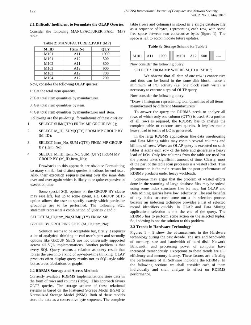
(IJCNS) International Journal of Computer and Network Security, Vol. 2, No. 5, May 2010
122
2.1 Difficult/ Inefficient to Formulate the OLAP Queries:
Consider the following MANUFACTURER_PART (MP) table:
Table 2: MANUFACTURER_PART (MP) M_ID Item_No QTY M101 A11 1000 M101 A12 500 M102 A11 800 M102 A12 900 M103 A12 700 M104 A12 200
Now, consider the following OLAP queries:
1: Get the total item quantity.
2: Get total item quantities by manufacturer.
3: Get total item quantities by item.
4: Get total item quantities by manufacturer and item. Following are the psudoSQL formulations of these queries:
1. SELECT SUM(QTY) FROM MP GROUP BY ( );
2. SELECT M_ID, SUM(QTY) FROM MP GROUP BY (M_ID);
3. SELECT Item_No, SUM (QTY) FROM MP GROUP BY (Item_No);
4. SELECT M_ID, Item_No, SUM (QTY) FROM MP GROUP BY (M_ID,Item_No);
Drawbacks to this approach are obvious: Formulating so many similar but distinct queries is tedious for end user. Also, their execution requires passing over the same data over and over again which is likely to be quite expensive in execution time.
Some special SQL options on the GROUP BY clause may ease life, but up to some extent, e.g. GROUP SETS option allows the user to specify exactly which particular groupings are to be performed. The following SQL statement represents a combination of Queries 2 and 3:
SELECT M_ID,Item_No,SUM(QTY) FROM MP
GROUP BY GROUPING SETS (M_ID,Item_No);
Solution seems to be acceptable but, firstly it requires a lot of analytical thinking at end user’s part and secondly options like GROUP SETS are not universally supported across all SQL implementations. Another problem is that every SQL Query returns a relation as query result that forces the user into a kind of row-at-a-time thinking. OLAP products often display query results not as SQL-style table but as cross tabulations or graphs.
2.2 RDBMS Storage and Access Methods Currently available RDBMS implementations store data in the form of rows and columns (table). This approach favors OLTP queries. The storage scheme of these relational systems is based on the Flattened Storage Model (FSM) or Normalized Storage Model (NSM). Both of these models store the data as a consecutive byte sequence. The complete
table (rows and columns) is stored in a single database file as a sequence of bytes, representing each row, with some free space between two consecutive bytes (figure 1). The space is left to accommodate future updates.
Table 3: Storage Scheme for Table 2
M101 A11 1000 M101 A12 500 ----
Now consider the following query: SELECT * FROM MP WHERE M_ID = ‘M101’;
We observe that all data of one row is consecutive and thus can be found in the same disk block, hence a minimum of I/O activity (i.e. one block read/ write) is necessary to execute a typical OLTP query. Now consider the following query: “Draw a histogram representing total quantities of all items manufactured by different Manufacturers” To answer the query the RDBMS needs to analyze all rows of which only one column (QTY) is used. As a portion of all rows is required, the RDBMS has to analyze the complete table to execute such queries. It implies that a heavy load in terms of I/O is generated. In the large RDBMS applications like data warehousing and Data Mining tables may contain several columns and billions of rows. When an OLAP query is executed on such tables it scans each row of the table and generates a heavy load of I/Os. Only few columns from the table are used but the process takes significant amount of time. Clearly, most of the part of the table scan processes is a wasted effort. This phenomenon is the main reason for the poor performance of RDBMS products under heavy workloads. Someone may argue that the problem of wasted efforts done in the scanning of large database files may be solved using some index structures like bit map, but OLAP and Data Mining queries have low selectivity. The real benefits of any index structure come out a in selection process because an indexing technique provides a list of selected record identifiers quickly. In OLAP and Data Mining applications selection is not the end of the query. The RDBMS has to perform some action on the selected tuples. So, indexing is not the solution to this problem. 2.3 Trends in Hardware Technology Figures 1 – 9 show the advancements in the Hardware technology during the past decade. The size and bandwidth of memory, size and bandwidth of hard disk, Network Bandwidth and processing power of computer have increased tremendously. Exceptions to these trends are I/O efficiency and memory latency. These factors are affecting the performance of all Software including the RDBMS. In the following sections we shall consider each of them individually and shall analyze its effect on RDBMS performance.
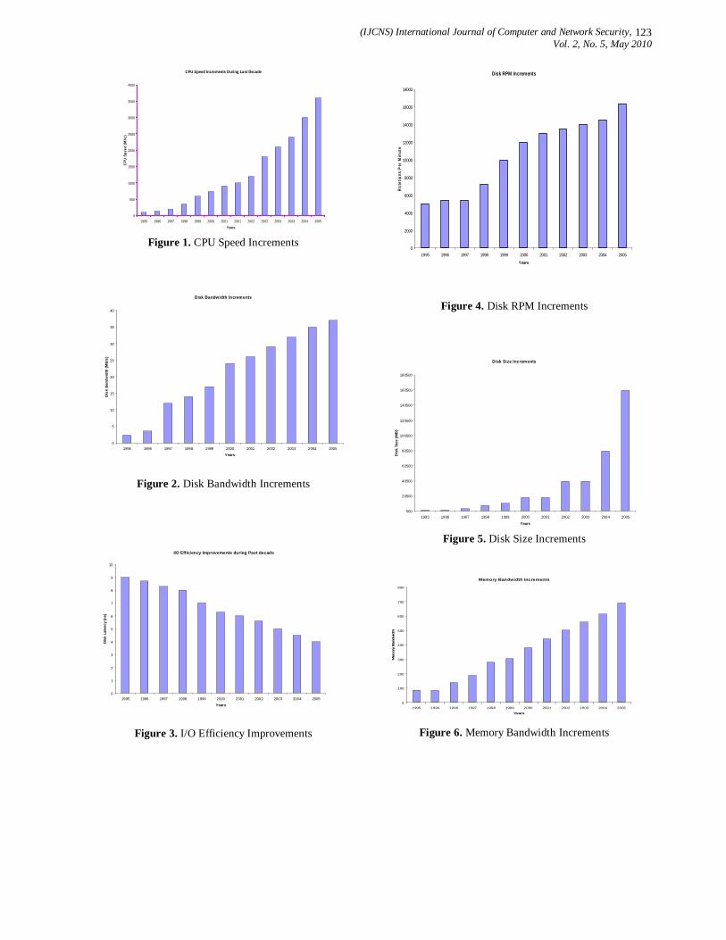
(IJCNS) International Journal of Computer and Network Security, Vol. 2, No. 5, May 2010
123
CPU Speed Increments During Last Decade
0
500
1000
1500
2000
2500
3000
3500
4000
1995 1996 1997 1998 1999 2000 2001 2001 2002 2002 2003 2003 2004 2005
Years
CPU
Spee
d (M
hz)
Figure 1. CPU Speed Increments
Disk Bandwidth Increments
0
5
10
15
20
25
30
35
40
1995 1996 1997 1998 1999 2000 2001 2002 2003 2004 2005
Years
Dis
k Ba
ndw
idth
(MB
/s)
Figure 2. Disk Bandwidth Increments
I/O Efficiency Improvements during Past decade
0
1
2
3
4
5
6
7
8
9
10
1995 1996 1997 1998 1999 2000 2001 2002 2003 2004 2005
Years
Disk
Lat
ency
(ns)
Figure 3. I/O Efficiency Improvements
Disk RPM Increments
0
2000
4000
6000
8000
10000
12000
14000
16000
18000
1995 1996 1997 1998 1999 2000 2001 2002 2003 2004 2005
Years
Rote
tions
Per
Min
ute
Figure 4. Disk RPM Increments
Disk Size Increments
500
20500
40500
60500
80500
100500
120500
140500
160500
180500
1995 1996 1997 1998 1999 2000 2001 2002 2003 2004 2005
Years
Dis
k Si
ze (M
B)
Figure 5. Disk Size Increments
Memory Bandwidth Increments
0
100
200
300
400
500
600
700
800
1995 1996 1996 1997 1998 1999 2000 2001 2002 2003 2004 2005
Years
Mem
ory
Ban
dwid
th
Figure 6. Memory Bandwidth Increments
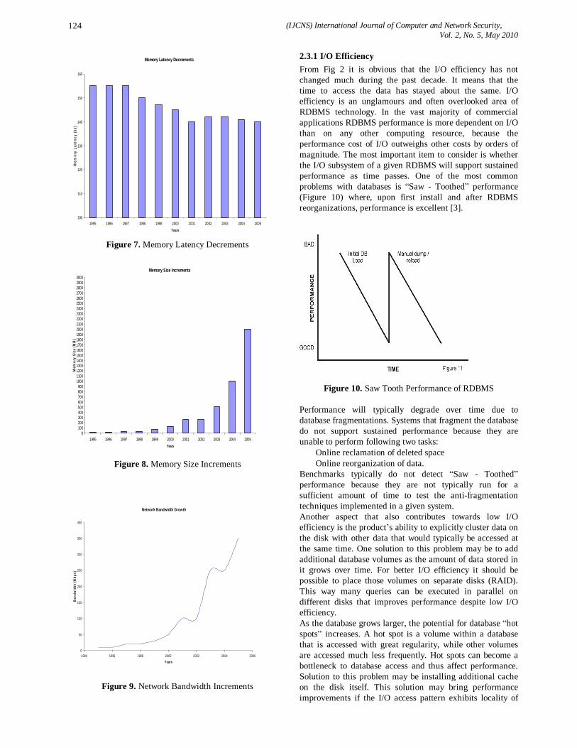
(IJCNS) International Journal of Computer and Network Security, Vol. 2, No. 5, May 2010
124
Memory Latency Decrements
100
110
120
130
140
150
160
1995 1996 1997 1998 1999 2000 2001 2002 2003 2004 2005
Years
Mem
ory
Late
ncy
(ns)
Figure 7. Memory Latency Decrements
Memory Size Increments
0100200300400500600700800900
100011001200130014001500160017001800190020002100220023002400250026002700280029003000
1995 1996 1997 1998 1999 2000 2001 2002 2003 2004 2005Years
Mem
ory
Size
(MB
)
Figure 8. Memory Size Increments
Network Bandwidth Growth
0
50
100
150
200
250
300
350
400
1994 1996 1998 2000 2002 2004 2006
Years
Band
wid
th (M
bps)
Figure 9. Network Bandwidth Increments
2.3.1 I/O Efficiency From Fig 2 it is obvious that the I/O efficiency has not changed much during the past decade. It means that the time to access the data has stayed about the same. I/O efficiency is an unglamours and often overlooked area of RDBMS technology. In the vast majority of commercial applications RDBMS performance is more dependent on I/O than on any other computing resource, because the performance cost of I/O outweighs other costs by orders of magnitude. The most important item to consider is whether the I/O subsystem of a given RDBMS will support sustained performance as time passes. One of the most common problems with databases is “Saw - Toothed” performance (Figure 10) where, upon first install and after RDBMS reorganizations, performance is excellent [3].
Figure 10. Saw Tooth Performance of RDBMS Performance will typically degrade over time due to database fragmentations. Systems that fragment the database do not support sustained performance because they are unable to perform following two tasks: Online reclamation of deleted space Online reorganization of data. Benchmarks typically do not detect “Saw - Toothed” performance because they are not typically run for a sufficient amount of time to test the anti-fragmentation techniques implemented in a given system. Another aspect that also contributes towards low I/O efficiency is the product’s ability to explicitly cluster data on the disk with other data that would typically be accessed at the same time. One solution to this problem may be to add additional database volumes as the amount of data stored in it grows over time. For better I/O efficiency it should be possible to place those volumes on separate disks (RAID). This way many queries can be executed in parallel on different disks that improves performance despite low I/O efficiency. As the database grows larger, the potential for database “hot spots” increases. A hot spot is a volume within a database that is accessed with great regularity, while other volumes are accessed much less frequently. Hot spots can become a bottleneck to database access and thus affect performance. Solution to this problem may be installing additional cache on the disk itself. This solution may bring performance improvements if the I/O access pattern exhibits locality of

(IJCNS) International Journal of Computer and Network Security, Vol. 2, No. 5, May 2010
125
reference and that is not the case with OLAP and Data Mining queries. 2.3.2 Network Latency:
Figure 11. Database CPU Demand
Low I/O efficiency is not the only form of I/O one should be concerned with. Network Latency is also equally important particularly in a Client – Server environment. An RDBMS should be able to move groups of objects (fields) to and from the Client when it is appropriate for the application. To optimally use Network Bandwidth, only objects that are requested by the Client should be returned. But what the RDBMS does is that, it passes all objects that reside together on a physical disk block to the Client, whether they are needed or not. This is really a serious problem with current RDBMS architecture. 2.3.3 Disk and Memory Bandwidth: From Figure 1 and 5 it is obvious that Disk and Memory bandwidths have increased tremendously during the past decade. In section 3.3.1 we have pointed out that I/O efficiency can be improved by installing RAID devices, but it may create another serious problem. It leads to poor performance if the total bandwidth of all RAID disks exceeds the memory bandwidth. As there is no way to scale the memory bandwidth, it can become a hurdle in installations with RAID and may contribute to poor RDBMS performance. 2.3.4 Memory Latency: Figure 7 shows the improvements in the Memory Latency. Clearly we can store more (Figure 5) and process faster but the time the memory takes to access the data has stayed about the same. Memory latency is the most urgent reason for low performance of RDBMS under heavy workloads. The only solution to this problem provided by vendors has been to install more cache memory. An application that has a memory access pattern that achieves a low cache hit rate can’t take the advantage of this solution. RDBMS applications that have this property are hash join and sorting [2], which are common operations in OLAP and Data Mining Queries.
2.3.5 CPU Utilization: Most of the researches relating database performance to processor have been carried out on multiprocessor platforms using OLTP workloads [10] [13]. Few studies evaluate database performance on multiprocessor platforms using both types of loads (i.e. OLTP and OLAP) [11]. All of the studies agree that the RDBMS behavior depends upon the nature of workloads (DSS or OLTP). With the development of www and emergence of DSS and CMS (Content Management Systems), RDBMS demand for CPU has doubled every 9-12 months according to Greg’s Law. At the same time processor speed has doubled every 18 months based on Moor’s Law. As shown in Figure 11, the gap between RDBMS demand and CPU speed is increasing [1]. Figure 12 shows CPU Utilization under OLTP workloads. A response time versus CPU utilization curve can be obtained using the following formula [6]: RESPONSE_TIME = ∑ Response_TIMES = ((QUEUE_LENGTH * SERVICE_TIME) + SERVICE_TIME) Figure 13 shows CPU Utilization Percentage versus response time. From figure 12 it is clear that at about 75% utilization, the growth of the queue length shifts from linear to asymptotic. The curve in the queue length graph also exists in response time graph. This is why we never want to run our CPUs in a steady state over 75%. We are seeing techniques such as speculative pre-fetch and multithreading in the processors but the RDBMS demand for CPU is still increasing. The main reason is that modern CPUs tend to be stalled for the majority of their time achieving the low utilization of their true power [5]. These CPU stalls are because of the memory latency. One solution to get the most out of modern CPUs may be that the performance intensive parts of program must contain only processor dependent instructions. This is a hard requirement and RDBMS applications can’t be designed using this principle. RDBMS instructions are more memory or I/O dependent, so RDBMS can’t take full advantage of modern CPUs.
Queue Length Vs. Processor Utilization
0
2000
4000
6000
8000
10000
12000
14000
16000
0 20 40 60 80 100 120Utilization (% Values)
Que
ue L
engt
h
Figure 12. CPU Utilization under OLTP workloads.

(IJCNS) International Journal of Computer and Network Security, Vol. 2, No. 5, May 2010
126
Response Time Vs. Processor Utilization
0
0.2
0.4
0.6
0.8
1
1.2
0 10 20 30 40 50 60 70 80 90 100
CPU Utilization (%)
Res
pons
e Time (S
ec.)
Figure 13. CPU Utilization Percentage versus response
time. We are seeing techniques such as speculative pre-fetch and multithreading in the processors but the RDBMS demand for CPU is still increasing. The main reason is that modern CPUs tend to be stalled for the majority of their time achieving the low utilization of their true power [5]. These CPU stalls are because of the memory latency. One solution to get the most out of modern CPUs may be that the performance intensive parts of program must contain only processor dependent instructions. This is a hard requirement and RDBMS applications can’t be designed using this principle. RDBMS instructions are more memory or I/O dependent, so RDBMS can’t take full advantage of modern CPUs. 3. Inability to Support Other Data Models In the RDBMS world the relational model and its query language (SQL) are most popular. Every entity is expressed in the form of table and the attributes of entity are the columns of the table. Relations between tables (Entities) are established by including the prime attribute (or a set of attributes which defines the primary key) of one table into another. This approach restricts the user to think in terms of tables, primary key, foreign key and other related terminologies. Clearly the thinking of an RDBMS database designer is narrow when it comes on expressing the data. Other data models like Object Oriented Model, Object – Relational Model and Multidimensional Data Model are becoming increasingly popular as they perform better under heavy workloads generated by DSS queries. We argue that if the RDBMS architecture is revised to support other data models too, then performance issues may be resolved up to some extent.
4. Conclusions and Future Work Relational Databases are the backbones of several Decision Support Systems and Content Management System in use. Despite the performance optimization found in today’s relational database systems, they are still not able to take full advantage of many improvements in the computing technology during the last decade. In this paper we have examined various aspects which contribute to the poor performance of relational databases when they support OLAP, Data Mining and Decision Support Systems. Several available solutions to address the performance issues and why they are insufficient have been discussed at length throughout the paper. We have also shown that expressing the queries related to these applications is a tough task in
the native language of relational databases and that the RDBMS tends to restrict the designer’s thinking around the row-column concept which shows the inability of relational databases to support any other data model. The results from our analysis suggest that hardware engineers must pay more attention to improve I/O, memory and network efficiencies. Memory latency has been identified as the most urgent reason contributing to the poor performance of RDBMS under heavy workloads. This is also responsible for long CPU stalls and can’t be cured by simply installing more caches. SQL must be revised and must be implemented to support other data models and should not bind the designer’s thinking around rows columns. Also it must be revised form the point of view of expressing the OLAP, Data Mining and DSS queries in an easy way. The RDBMS kernel must be rewritten to take the full advantage of the hardware trends seen during the last decade. References [1] X. CUI, “A Capacity Planning Study of DBMS With
OLAP Workloads”, Masters Thesis, School of Computing, Queen’s University, Ontario, Canada October 2003.
[2] S. Manegold, P. Boncz and M. Kersten “Optimizing Join on Modern Hardware” IEEE TKDE, 14(4), July 2002.
[3] H. Zawawy “Capacity Planning for DBMS Using Analytical Modeling”, Master Thesis, School of Computing, Queen’s University, Ontario, Canada, December 2001.
[4] S. Manegold, P. Boncz and M. Kersten “What Happens During a Join? Dissecting CPU and Memory Optimization Effects” In Proceedings of VLDB Conference, Cairo, Egypt, July 2000.
[5] Anastassia Ailamaki, D.J. DeWitt, M.D. Hill, and D.A. Wood “DBMSs on a modern processor: Where Does Time Go?” In Proceedings of the 25th VLDB Conference, Edinburg, Scotland, 1999.
[6] E. Whalen “Teach Yourself Oracle 8 in 21 Days”, Macmillan Computer Publishing, 1998, USA.
[7] J. Vijavan “Capacity Planning More Vital Than Ever”, Computer World, pp 1, February 1999.
[8] PC Quest Magazine www.pcquest.com.
[9] Rain Maker Group Whitepapers and Tools Library available from www.rainmakerworks.com.
[10] K. Keeton, D.A. Patterson, Y.Q. He, R.C. Raphael and W.E. Baker “Performance Characterization of a Quad Pentium Pro SMP using OLTP Workloads.” In Proceedings of the 25th International Symposium on Computer Architecture, pages 15 – 26, Barcelona, Spain, June 1998.
[11] P. Ranganathan, K. Gharachorloo, S. Adve and L. Barroso “Performance of Database Workloads on Shared Memory Systems with Out-of-Order
(IJCNS) International Journal of Computer and Network Security, Vol. 2, No. 5, May 2010
127
Processors.” In Proceeding of the 8th International Conference on Architectural Support for Programming Languages and Operating Systems, San Jose, California, October 1998.
[12] D.A. Menasce, V.A.F. Almeida “Challenges in Scaling e-Business Sites”, In Proceedings of Computer Measurement Group Conference, 2000.
[13] L.Lo, L.A. Barroso, S.J. Eggers, K.Gharachorloo, H.M. Levy and S.S. Parekh, “An Analysis of Database Workload Performance on Simulated Multithreaded Processors.” In Proceedings of the 25th International Symposium on Computer Architecture, pages 39 – 50, Barcelona, Spain, June1998.
Authors Profile
Dr. Sami M. Halawani Received the M.S. degree in Computer Science from the University of Miami, USA, in 1987. He received the Professional Applied Engineering Certificate from The George Washington University, USA, in 1992. He earned the Ph.D. degree in Information Technology from the George Mason University, USA in 1996. He is a faculty
member of the College of Computing and Information Technology, King Abdul aziz University, Jeddah, Saudi Arabia. He is currently working as the Dean for Graduate Studies and Research. He has authored/ co-authored many publications in journals/conference proceedings.
Dr. Ibrahim Albidewi is an Associate Professor at the department of Information Systems, Faculty of Computing and Information Technology, King Abdualziz University, Jeddah. He was the director of Computer Center at King Abdulaziz University. His experience and publications are in the area of image processing,
new vision of programming, expert system, computer education, and management of information centers. 1986: Bachelor degree from Department of Islamic Economic, College of Islamic Studies, University of Umm Al-Qura, 1989: Master degree from Department of Computer Science, College of Sciences, swansea University, 1993: Doctorate degree from Electrical and Electronics Eng, College of Engineering, Swansea University.
Jahangir Alam graduated in science from Meerut University, Meerut in the year 1992 and received Master degree in Computer Science and Applications from Aligarh Muslim University, Aligarh in the year 1995 and Master in Technology (M.Tech) Degree in Computer Engineering from
JRN Rajasthan Vidyapeeth University, Udaipur, Rajasthan, in the year 2008. He is currently working towards his Ph.D. in Computer Engineering from Thapar University, Patiala. He is also serving as an Assistant Professor in University Women’s Polytechnic, Faculty of Engineering and Technology at Aligarh Muslim University, Aligarh. His areas of interest include Interconnection Networks, Scheduling and Load Balancing, Computer Communication Networks and Databases. He has authored/ co-authored over 12 publications in journals/conference proceedings
Zubair Khan received his Bachelor Degree in Science and Master of Computer Application Degree from MJP Rohilkhand University Bareilly, India in 1996 and 2001 respectively and also Master in Technology (M.Tech) Degree in Computer Science and Engineering from Uttar Pardesh Technical University in the year 2008. He is currently pursuing his P.hd in
computer science and Information Technology from MJP Rohilkhand University Bareilly, UP India. He also worked as a senior lecturer in JAZAN University Kingdom of Saudi Arbia. He is also servicing as Reader in the Department Of Computer Science and Engineering Invertis Institute of Technology Bareilly, India. His areas of interest include data mining and warehousing, parallel systems and computer communication networks. He is an author/ co-author of more than 15 international and national publications in journals and conference proceedings.
(IJCNS) International Journal of Computer and Network Security, Vol. 2, No. 5, May 2010
128
Cluster Based Hierarchical Routing Protocol For Wireless Sensor Network
Md. Golam Rashed1, M. Hasnat Kabir2, Muhammad Sajjadur Rahim3, Shaikh Enayet Ullah4
1 Department of Electronic and Telecommunication Engineering (ETE),
University of Development Alternative (UODA), Bangladesh .
2,4 Department of Information and Communication Engineering
University of Rajshahi, Rajshahi-6205, Bangladesh. 3School of Information Engineering, University of Padova, Italy.
Abstract: The efficient use of energy source in a sensor node is most desirable criteria for prolong the life time of wireless sensor network. In this paper, we propose a two layer hierarchical routing protocol called Cluster Based Hierarchical Routing Protocol (CBHRP). We introduce a new concept called head-set, consists of one active cluster head and some other associate cluster heads within a cluster. The head-set members are responsible for control and management of the network. Results show that this protocol reduces energy consumption quite significantly and prolongs the life time of sensor network as compared to LEACH.
Keywords: WSN, Cluster, Routing Protocols
1. Introduction
Wireless Sensor Networks (WSN) consists with huge tiny sensors that are arranged in spatially distributed terrain. Due to a large number of applications such as security, agriculture, automation and monitoring, WSN has been identified as one of the pioneer technique in 21st century. The deployment and maintenance of the small sensor nodes should be straightforward and scalable when they are useless. But the small sensor nodes are usually inaccessible to the user, and thus replacement of the energy source is not feasible. There are some technical constrains also in microsensor node such as low energy in battery and processing speed etc. This limitation should be overcome as much as possible to use the node in wireless sensor network. The source of energy in sensor is a main constrain among them [1]. It can be minimized by increasing the density of energy in conventional energy sources [2],[3]. One of the elegant ways to prolong the lifetime of the network is to be reduced energy consumption in sensor nodes. This idea has been applied many research [4],[5] to increase the life time of the network. Cluster based Low-Energy Adaptive Clustering Hierarchy (LEACH) is an attractive routing protocol that disperses the energy load among the sensor nodes [6],[7],[8]. The improvements of LEACH have been presented elsewhere [9],[10],[11]. Proposed protocol is another approach to improve of LEACH protocol by
reducing energy consumption and prolong the life time of the network.
2. The Proposed Approach (CBHRP)
In this paper an optimum energy efficient cluster based hierarchical routing protocol for wireless sensor network is proposed, which is a two layer protocol where a number of cluster cover the whole region. Proposed protocol introduces a concept of head-set instead of a cluster head. At one time, only one member of head-set is active and the remaining are in sleep mode. Several states of a node are found in this protocol such as- candidate state, non-candidate state, active state, associate state, and passive associate state. This protocol divides the network into a few real clusters including an active cluster head and some associate cluster heads. For a given number of data collecting nodes, the head-set members are systematically adjusted to reduce the energy consumption, which increases the network life.
3. Architecture of CBHRP
In the proposed model, the number of clusters k and nodes n are pre-determined for the wireless sensor network. Iteration consists of two stages: an election phase, and a data transfer phase. At the beginning of election phase, a set of cluster heads are chosen on random basis. These cluster heads send a short range advertisement broadcast message. The sensor nodes receive the advertisements and choose their cluster heads based on the signal strength of the advertisement messages. Each sensor node sends an acknowledgment message to its cluster head. Moreover, in each iteration, the cluster heads choose a set of associate heads based on the signal strength of the acknowledgments. A head-set consists of a cluster head and the associates. The head-set member is responsible to send messages to the base station. Each data transfer phase consists of several epochs. Each member of head-set becomes a cluster head once during an epoch. A round consists of several iterations. In one round, each sensor node becomes a member of head-set for one time. All the head-set members share the same time slot to transmit their frames.
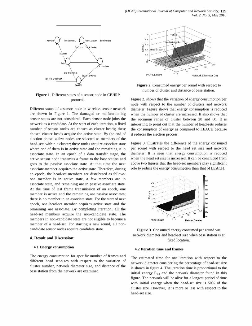
(IJCNS) International Journal of Computer and Network Security, Vol. 2, No. 5, May 2010
129
Figure 1. Different states of a sensor node in CBHRP protocol.
Different states of a sensor node in wireless sensor network are shown in Figure 1. The damaged or malfunctioning sensor states are not considered. Each sensor node joins the network as a candidate. At the start of each iteration, a fixed number of sensor nodes are chosen as cluster heads; these chosen cluster heads acquire the active state. By the end of election phase, a few nodes are selected as members of the head-sets within a cluster; these nodes acquire associate state where one of them is in active state and the remaining is in associate state. In an epoch of a data transfer stage, the active sensor node transmits a frame to the base station and goes to the passive associate state. At that time the next associate member acquires the active state. Therefore, during an epoch, the head-set members are distributed as follows: one member is in active state, a few members are in associate state, and remaining are in passive associate state. At the time of last frame transmission of an epoch, one member is active and the remaining are passive associates; there is no member in an associate state. For the start of next epoch, one head-set member acquires active state and the remaining are associate. By completing iteration, all the head-set members acquire the non-candidate state. The members in non-candidate state are not eligible to become a member of a head-set. For starting a new round, all non-candidate sensor nodes acquire candidate state.
4. Result and Discussion:
4.1 Energy consumption
The energy consumption for specific number of frames and different head set-sizes with respect to the variation of cluster number, network diameter size, and distance of the base station from the network are examined.
050
100150
200
0
20
40
600
0.2
0.4
0.6
0.8
1
Network Diameter (m)# Of Clusters
Ein
it(J)
Head-set size=4
Head-set size=2
LEACH
Figure 2. Consumed energy per round with respect to number of cluster and distance of base station.
Figure 2. shows that the variation of energy consumption per node with respect to the number of clusters and network diameter. Figure shows that energy consumption is reduced when the number of cluster are increased. It also shows that the optimum range of cluster between 20 and 60. It is interesting to point out that the number of head-sets reduces the consumption of energy as compared to LEACH because it reduces the election process.
Figure 3. illustrates the difference of the energy consumed per round with respect to the head set size and network diameter. It is seen that energy consumption is reduced when the head set size is increased. It can be concluded from above two figures that the head-set members play significant role to reduce the energy consumption than that of LEACH.
Figure 3. Consumed energy consumed per round wrt network diameter and head-set size when base station is at
fixed location.
4.2 Iteration time and frames
The estimated time for one iteration with respect to the network diameter considering the percentage of head-set size is shown in figure 4. The iteration time is proportional to the initial energy Einit and the network diameter found in this figure. The network will be alive for a longest period of time with initial energy when the head-set size is 50% of the cluster size. However, it is more or less with respect to the head-set size.

(IJCNS) International Journal of Computer and Network Security, Vol. 2, No. 5, May 2010
130
Figure 4. Time for iteration with respect to network diameter and head-set size.
Figure 5. Time for iteration with respect to number of clusters and network diameter.
Figure 5 shows a graph that illustrates the estimated time for one iteration with respect to the number of clusters and network diameter. The number of cluster does not affect on iteration time for a particular network diameter. However, the head-set size plays a significant role to increase the iteration time. In contrast to LEACH, iteration time is increased by several times for a given number of head-set.
100110
120130
140150
140
160
180
2000
1
2
3
4
5
x 104
DiameterDistance
# of
Fra
mes
Head set size=5
Head set size=3
LEACH
Figure 6. Number of frames transmission per iteration with respect to distance of BS and network diameter.
Data transmission in a wireless network is one of the most important issues. It is a measuring tool of a network suitability and perfectness. Our results show that the proposed method is able to transmit higher data frame in contrast to LECAH for the same dimension and distance of BS. While, head-set size is responsible to increase the data frame transmission. On the other hand, it is clearly found that the transmission rate slightly decreases with respect to the distance of BS. Figure 6 shows the number of frames transmitted with respect to network diameter and distance from BS.
5. Conclusion
An effective routing protocol is designed and tested it performances to overcome some present limitation of WSN. Introducing head-set concepts instead of only one cluster head within a cluster, our results show the better performance than that of LEACH in context of energy consumption, frame transmition and the life time of the sensor network.
References
[1] K. Pister, “On the limits and applications of MEMS sensor networks”, Defense Science Study Group report, Institute for Defense Analysis, Alexandria, VA.
[2] J. M. Rabaey, M. J. Ammer, J. L. da Silva, D. Patel, S. Roundy, “PicoRadio supports ad hoc ultra-low power wireless networking, IEEE Computer, July 2000, pp. 42-48.
[3] D. Timmermann, “Smart environments”, Invited Paper, Ladenburger Diskurs, Ladenburg, January 2001.
[4] L. Zhong, R. Shah, C. Guo, J. Rabaey, “An ultra low power and distributed access protocol for broadband wireless sensor networks”, IEEE Broadband Wireless Summit, Las Vegas, May 2001.
[5] V. Rodoplu, T. H. Meng, “Minimum energy mobile wireless networks”, IEEE Jour. Selected Areas Comm., August 1999, pp. 1333-1344.
[6] W. Heinzelman, A. Sinha, A. Wang, A. Chandrakasan, “Energyscalable algorithms and protocols for wireless microsensor networks”, Proc. International Conference on Acoustics, Speech, and Signal Processing (ICASSP '00), June 2000.
[7] W. Heinzelman, A. Chandrakasan, and H.Balakrishnan, “Energy-efficient communication protocol for wireless microsensor Networks”, Proceedings of the 33rd International Conference on System Sciences (HICSS ’00), January 2000.
[8] S. Lindsey, C. Raghavendra, K. Sivalingam, “Data gathering in sensor networks using the energy*delay metric”, Proc. of the IPDPS Workshop on Issues in Wireless Networks and Mobile Computing, April 2001.
[9] E. B. Heinzelman, A. P. Chandrakasan, and H. Balakrishnan, “An Application-Specific Protocol Architecture for Wireless Microsensor Networks”, IEEE Transactions On Woreless Communications, Vol. 1, No. 4, October 2002.
(IJCNS) International Journal of Computer and Network Security, Vol. 2, No. 5, May 2010
131
[10] A. Manjeshwar and D.P. Agrawal, "APTEEN: A Hybrid Protocol for Efficient Routing and Comprehensive Information Retrieval in Wireless Sensor Networks," in the Proceeding of the 2nd International Workshop on Parallel and Distributed Computing Issues in Wireless Networks and Mobile Computing, Ft.Lauderdale, FL, April 2002.
[11] Wang Wei, “Study on Low Energy Grade Routing Protocols of Wireless Sensor Networks”, Dissertation, Hang Zhou, Zhe Jiang university,2006.
Authors Profile Md. Golam Rashed received the B.Sc. and M.Sc. degree in Information and Communication Engineering from University of Rajshahi, Bangladesh in 2008 and 2009, respectively. He is currently working as a Lecturer in the department of Electronic and Telecommunication Engineering(ETE), University of Development Alternative (UODA), Bangladesh . M. Hasnat Kabir received the B.Sc. and M.Sc. degree in Applied Physics and Electronics from University of Rajshahi, Bangladesh in 1995 and 1996, respectively. He has completed his PhD from Kochi University of Technology, Japan in 2007. Now he is working as an Assistant Professor in the dept. of Information and Communication Engineering, University of Rajshahi, Bangladesh. M. Sajjadur Rahim received his B.Sc. (Engg.) degree in Electrical and Electronic Engineering from Bangladesh University of Engineering and Technology, Bangladesh and Master of Engineering degree in Information Science and Systems Engineering from Ritsumeikan University, Japan in 1999 and 2006, respectively. He is working as an Assistant Professor in the dept. of Information and Communication Engineering, University of Rajshahi, Bangladesh. At present, he is pursuing his PhD degree in the School of Information Engineering at the University of Padova, Italy on study leave. Shaikh Enayet Ullah received the B.Sc. and M.Sc. degree in Applied Physics and Electronics from University of Rajshahi, Bangladesh. He has completed his PhD from Jahangirnagor University, Bangladesh. He is currently working as a Professor and Chairman of the dept. of Information and Communication Engineering, University of Rajshahi, Bangladesh.
(IJCNS) International Journal of Computer and Network Security, Vol. 2, No. 5, May 2010
132
Analysis of Subband Speech Enhancement Technique for Digital Hearing Aids
D. Deepa1, Dr. A. Shanmugam2
Bannari Amman Institute o Technology, Sathyamangalam, Tamilnadu, India
1 [email protected], 2 [email protected]
Abstract: Hearing impairment is the number one chronic disability affecting people in the world. Many people have great difficulty in Understanding speech with background noise. Speech Enhancement plays a vital role in such situations. Random noise will disturb the signal between speaker and the listener. Therefore the background noise has to be removed from the noisy speech signal to increase the signal intelligibility and to reduce the listener fatigue. The proposed approach is a speech enhancement method based on the preprocessed sub band spectral subtraction method, and the preprocessing is done by using partial differential equation. This method provides a greater degree of flexibility and control on the noise subtraction levels that reduces artifacts in the enhanced speech, resulting in improved speech quality and intelligibility.
Key words- Sub band Spectral Subtraction, Partial differential equation, Adaptive noise estimation, Signal to Noise ratio, IS distance.
1. Introduction Understanding speech with background noise is difficult even for normal hearing people, for the people with hearing disability it is one of the major problem which is to be reduced. This is especially true for a large number of elderly people and the sensorineural impaired persons. Several investigations on speech intelligibility have demonstrated that subjects with sensorineural loss may need a 5-15 dB higher signal-to-noise ratio than the normal hearing subjects. Recent statistics of the hearing impaired patients applying for a hearing aid reveal that 20% of the cases are due to conductive losses, more than 50% are due to sensorineural losses, and the rest 30% of the cases are of mixed origin. Presenting speech to the hearing impaired in an intelligible form remains a major challenge in hearing-aid research today. In single channel system, speech enhancement is a challenging on because reference noise signal will not be available for enhancement. The clean speech cannot be processed prior to being affected by the noise. This is one of the most difficult situations in speech enhancement for a single channel system. The conventional power spectral subtraction method for single channel speech enhancement substantially reduces the noise levels in the noisy speech but this will introduce musical noise.
The proposed method is a preprocessed sub band spectral subtraction method of speech enhancement and the preprocessing technique is using partial differential equation. In this method first the input noisy speech signal is enhanced using PDE by taking the adjacent samples and calculating the gradient, influencing coefficients and then the output of this process is applied to the input for sub band spectral subtraction method. The noise estimate in spectral
subtraction is updated by averaging the noise speech spectrum using a time and frequency dependant smoothing factor, which is adjusted based on signal presence probability in sub bands. Signal presence is determined by computing the ratio of the noisy speech power spectrum to its local minimum, which is computed by averaging past values of the noisy speech power spectra with a look-ahead factor. This local minimum estimation algorithm adapts very quickly to highly non stationary noise environments. By using this noise estimation algorithm in this method outperforms the standard power spectral subtraction method resulting in superior speech quality and largely reduced musical noise in single channel system for both stationary and non stationary noise environments.
2. Partial Differential Equation Technique Input noisy speech signal affected by additive background noise can be enhanced by this method. First step in speech enhancement using PDE is to obtain the gradient (g) of each sample in noisy speech signal using the samples before and after the current sample.
),(),(),(),(
txStxxSgtxStxxSg
b
f
−∆+=
−∆−= --------- (2.1)
Where, S(x,t) is the noisy speech signal, Δx is the sampling rate. After the gradient is calculated the influencing coefficients in each directions of the current sample are computed.
2
2
1
1
1
1
+
=
+
=
kg
IC
kg
IC
bb
ff
---------- (2.2)
Where, ICf is the Forward influencing coefficient and ICb is the backward influencing coefficient. In the equation (2) ‘k’ is constant value between 1 and 100. From the above calculated influencing coefficients and gradients the speech signal is enhanced using
)(),(),( bbff ICgICgttxSttxS +∆+=∆+ ------- (2.3)
In the above equations S(x,t) is the input noisy speech signal, Δt is a coefficient between 0.1 t0 0.6 representing the step of noise reduction in each iteration. The output of the signal is again processed by applying into the algorithm of

(IJCNS) International Journal of Computer and Network Security, Vol. 2, No. 5, May 2010
133
Sub band spectral subtraction method to reduce the non stationary noise.
3. Sub band Spectral Subtraction method Sub band Spectral subtraction method is the
frequency dependent processing of the Spectral Subtraction procedure. This method offers better quality [9] of the enhanced speech with reduced residual noise. This approach has been justified due to variation in signal to noise ratio across the speech spectrum. White Gaussian noise has a flat spectrum, where as the real world noise is not flat. The noise spectrum does not affect the speech signal uniformly over the whole spectrum; some frequencies are affected more adversely than others.
To take into account the fact that colored noise affects the speech spectrum differently at various frequencies, we use this approach to spectral subtraction. The speech spectrum is divided into non-overlapping bands, and spectral subtraction is performed independently in each band. The estimate of the clean speech spectrum in the ith band is obtained by:
2
(k)iDiiα2(k)Y2
(k)iS δ−= ; iekib ≤≤
(3.1) where bi and ei are the beginning and ending frequency bins of the ith frequency band, a i is the over subtraction factor and δi is the band subtraction factor. Over subtraction factor provides a degree of control over the noise subtraction level in each band, the use of multiple frequency bands and the use of the δi weights provide an additional degree of control within each band. 4. Noise estimation
Noise estimation plays an important role in this work of speech enhancement. For an efficient noise estimation algorithm the resultant signal estimation will have great accuracy. 4.1. Adaptive noise-estimation algorithm
Several noise-estimation algorithms have been proposed for speech enhancement applications [2] [3] [4] [5] [6]. The main drawback of most of the noise estimation algorithms is that they are either slow in tracking sudden increases of noise power or that they are over estimating the noise energy resulting in speech distortion.
In the adaptive method the smoothed power spectrum of noisy speech is computed using the following first-order recursive equation:
2k),Y(g)(1k)1,gP(α),( αα −+−=kP --------(4.1)
where P(α,k) is the smoothed power spectrum, α is the frame index, k is the frequency index, |Y(α,K)| 2 is the short-time power spectrum of noisy speech and g is a smoothing constant. The proposed algorithm is summarized in the following steps. 4.1.1 Speech present and speech absent frames.
In any speech sentence there are pauses between words which do not contain any speech, those frames will
contain only background noise. The noise estimate can be updated by tracking those noise only frames. To identify those frames, a simple procedure is used which calculates the ratio of noisy speech power spectrum to the noise power spectrum at 3 different frequency bands in each frame and the sampling frequency respectively. If all the three ratios are smaller than the threshold that frame is concluded as a noise only frame, otherwise , if any one or all the ratios are greater than threshold that frame is considered as speech present frame. The noise estimate is updated in speech absent frames with a constant smoothing factor. In speech present frames the noise is updated by tracking the local minimum of noisy speech and the deciding speech presence in each frequency bin separately using the ration of noisy speech power to its local minimum. 4.1.2 The minimum of noisy speech
In our method for tracking the minimum of the noisy speech by continuously averaging past spectral values. In this algorithm if the value of the noisy speech spectrum in the present frequency bin is greater than the minimum value of previous frequency bin then the minimum value is updated, else the previous value is maintained as it is. 4.1.3. Detection of Speech-presence frames
The approach taken to determine speech presence in each frequency bin is similar to the method used in [4]. Let the ratio of noisy speech power spectrum and its local minimum be defined as
k),(minPk),P(k),(rS α
αα = -------- (4.2)
This ratio is compared with a frequency dependent threshold, and if the ratio is found to be greater than the threshold, it is taken as a speech-present frequency bin else it is taken as a speech-absent frequency bin. This is based on the principle that the power spectrum of noisy speech will be nearly equal to its local minimum when speech is absent. Hence the smaller the ratio is in (6), the higher the probability that it will be a noise-only region and vice versa. Note that in [4], a fixed threshold was used in place of threshold.
From the above rule, the speech-presence probability, p(α,K), is updated using the following first-order recursion: p(α,k) = a p(α -1,k) + (1- a ) I (α,k) ------- (4.3) where a is a smoothing constant. Note that the above recursion implicitly exploits the correlation for speech presence in adjacent frames. This may result in slight overestimate of the noise spectrum but will not likely have much effect on the enhanced speech. 4.1.4. Calculation of Smoothing Constants
Using the above speech-presence probability estimate, we compute the time–frequency dependent smoothing factor as follows [4]. a(α,K) = d + ( 1- d) p(α,k) ------------ (4.4) where d is a constant. Note that a(α,K) takes values in the range of d ≤ a(α,K) ≤ 1. 4.1.5 Updation of noise spectrum estimate Finally, after computing the frequency- dependent smoothing factor a(α,k), the noise spectrum estimate is updated as

(IJCNS) International Journal of Computer and Network Security, Vol. 2, No. 5, May 2010
134
D(α,k) = a(α,k) D(α -1,k) + (1- a(α,k) ) |Y(α,K)| 2 -----(4.5)
where D(α,k) is the estimate of the noise power spectrum. Finally the noise spectrum estimate is updated using the time–frequency dependent smoothing factor.
For each frequency band this estimated noise is subtracted from the input noisy speech signal, finally the output of each band is combined by using OLA method to get an estimate of clean speech (Enhanced speech). 5. Objective measures for performance evaluation
Objective measures are based on a mathematical comparison of the original and processed speech signals. It is desired that the objective measures be consistent with the judgement of the human perception of speech [7]. However, it has been seen that the correlation between the results obtained by objective measures are not highly correlated with those obtained by subjective measures. The signal-to-noise ratio (SNR) and the Itakura-Saito (IS) measure are two of the most widely used objective measures. 5.1 Signal-to-noise ratio (SNR)
The SNR is a popular method to measure speech quality. As the name suggests, it is a calculated as the ratio of the signal to noise power in decibels. If the summation is performed over the whole signal length, the operation is called global SNR.
[ ]
∑ −
∑=
n
2(n)SS(n)n
(n)2S
1010logdBSNR ----------(5.1)
5.2 Itakura - Saito Distance
Itakura - Saito measure is one of the distance measures. Lower the IS distance, better will be the quality of speech (i.e. minimum phase difference between clean and enhanced signal). The average Itakura-Saito measure across all speech frames of the given sentence will be computed to evaluate the spectral noise subtraction algorithm.
Raa
baRbabad r
r )()(),( −−= ----------(5.2)
where a is the vector for the prediction coefficients of the clean speech signal, vector R is the autocorrelation matrix of the clean speech signal and vector b is the prediction coefficients of the enhanced signal.
6. Experimental Results
Test samples are taken from SpEAR (Speech Enhancement Assessment Resource) database of CSLU (Center for Spoken Language Understanding). Time domain Results : Sample 1
Figure 1 a. Car Clean Signal
Figure 1 b. Noisy Car Signal
Figure1 c. Enhanced Car Signal
Sample 2:
Figure 2 a. Clean speech
Figure2 b. White stationary Noisy speech
Figure 2 c. Enhanced speech
Frequency Domain Analysis:
Power Spectral Density of Reference Clean signal, Noisy Signal and the Enhanced Signals were obtained and compared
0 20 40 60 80 100 120 1400
0.1
0.2
0.3
0.4
0.5
0.6
0.7
Time
Amplitu
de
PSD COMPARISON
NOISY SIGNALENHANCED SIGNALdata3
Figure 3. PSD plot of Cellular noisy, clean and Enhanced signal
Inference for Fig3: Power spectrum density of the enhanced signal is close to the power spectrum magnitude of clean signal.
0 20 40 60 80 100 120 1400
0.05
0.1
0.15
0.2
0.25
0.3
0.35
Freque ncy
PSD
PSD Comparison of White Stationary Noisy s ignal
Noisy SignalClean SignalEnhanced Signal
Figure 4. PSD comparisons for White Stationary Noisy
signal Inference: Figure 4 shows the Power spectral density comparison for White stationary noisy signal. The output shows that the stationary noise signal in higher frequency range (i.e. 40 to 130) is minimized
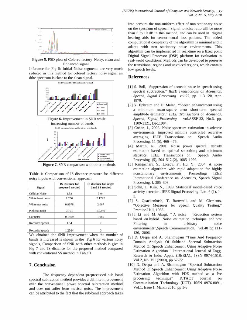
(IJCNS) International Journal of Computer and Network Security, Vol. 2, No. 5, May 2010
135
0 20 40 60 80 100 120 1400
0.05
0.1
0.15
0.2
0.25
0.3
0.35
Frequency
PSD
PSD COMPARISON
NOISY SIGNALENHANCED SIGNALCLEAN SIGNAL
Figure 5. PSD plots of Colored factory Noisy, clean and
Enhanced signal Inference for Fig 5: Initial Noise segments are very much reduced in this method for colored factory noisy signal an dthe spectrum is close to the clean signal.
SNR O btaine d for different num be r of bands
-100
1020304050
Single band
2 bands
4 bands
8 bands Figure 6. Improvement in SNR while
increasing number of bands SNR comparison with other methods
-10
0
10
20
30
40
50
Whit
e stationa
ry 0db
noisy s
igna
l
White st
ationa
ry 7db
noisy sig
nal
White bur
sting
0db
noisy
Signa
l
White bursti
ng 3db
noisy
Signa
l
Pink
statio
nary
0db no
isy signa
l
Pink
stationa
ry 6d
b no
isy signa
l
Car n
oisy
(female)
signa
l
Cellu
lar 0
db nois
y sig
nal
Reco
rded
sam
ple1
(yok
vet)
Typa of Noise
SNR
Single band4 bandsSS methodDEKF Algorihm
Figure 7. SNR comparison with other methods Table 1: Comparison of IS distance measure for different noisy inputs with conventional approach
We obtained the SNR improvement when the number of bands is increased is shown in the Fig 6 for various noisy signals, Comparison of SNR with other methods is give in Fig 7 and IS distance for the proposed method compared with conventional SS method in Table 1.
7. Conclusion
The frequency dependent preprocessed sub band spectral subtraction method provides a definite improvement over the conventional power spectral subtraction method and does not suffer from musical noise. The improvement can be attributed to the fact that the sub-band approach takes
into account the non-uniform effect of non stationary noise on the spectrum of speech. Signal to noise ratio will be more than 6 to 10 dB in this method, and can be used in digital hearing aids for sensorineural loss patients. The added computational complexity of the algorithm is minimal and it adapts with non stationary noise environments. This algorithm can be implemented in real-time on a fixed point Digital Signal Processor (DSP) platform for evaluation in real-world conditions. Methods can be developed to preserve the transitional regions and unvoiced regions, which contain low speech levels.
References
[1] S. Boll, “Suppression of acoustic noise in speech using spectral subtraction,” IEEE Transactions on Acoustics, Speech, Signal Processing vol.27, pp. 113-120, Apr. 1979.
[2] Y. Ephraim and D. Malah, “Speech enhancement using a minimum mean-square error short-term spectral amplitude estimator,” IEEE Transactions on Acoustics, Speech, Signal Processing vol.ASSP-32, No.6, pp. 1109-1121, Dec.1984.
[3] Cohen, I., 2003. Noise spectrum estimation in adverse environments: improved minima controlled recursive averaging. IEEE Transactions on Speech Audio Processing. 11 (5), 466–475.
[4] Martin, R., 2001. Noise power spectral density estimation based on optimal smoothing and minimum statistics. IEEE Transactions on Speech Audio Processing (5), 504–512.(2), 1085–1099.
[5] Rangachari, S., Loizou, P., Hu, Y., 2004. A noise estimation algorithm with rapid adaptation for highly nonstationary environments. Proceedings IEEE International Conference on Acoustics, Speech Signal Processing. I, 305–308.
[6] Sohn, J., Kim, N., 1999. Statistical model-based voice activity detection. IEEE Signal Processing. Lett. 6 (1), 1–3.
[7] S. Quackenbush, T. Barnwell, and M. Clements, “Objective Measures for Speech Quality Testing,” Prentice-Hall, 1988.
[8] J. Li and M. Akagi, “ A noise Reduction system based on hybrid Noise estimation technique and post Filtering in arbitrary noise environments”,Speech Communication, vol.48 pp 111- 126, 2006.
[9] D. Deepa and A. Shanmugam “Time And Frequency Domain Analysis Of Subband Spectral Subtraction Method Of Speech Enhancement Using Adaptive Noise Estimation Algorithm ” International Journal of Engg. Research & Indu. Appls. (IJERIA)., ISSN 0974-1518, Vol.2, No. VII (2009), pp 57-72
[10] D. Deepa and A. Shanmugam “Spectral Subtraction Method Of Speech Enhancement Using Adaptive Noise Estimation Algorithm with PDE method as a Pre processing technique” ICTACT Journal on Communication Technology (IJCT). ISSN 0976-0091, Vol.1, Issue 1, March 2010, pp 1-6
Signal IS Distance for
proposed method IS distance for single
band SS method
Cellular Noise 1.53 3.04 White burst noise 1.256 2.1722
White stat noise 0.9978 2.067
Pink stat noise 0.791 1.0246
Car noise 0.1569 1.989
Recorded speech 1.54 0
Recorded speech 1.2564 0
(IJCNS) International Journal of Computer and Network Security, Vol. 2, No. 5, May 2010
136
An improved low voltage, low power class AB operational transconductance amplifier for mobile
Applications
M.SanthanaLakshmi1 and Dr. P.T. Vanathi 2
1PSG College of Technology, Peelamedu, Coimbatore, India
2PSG College of Technology, Peelamedu, Coimbatore, India
Abstract: This paper presents a 1.1V Class AB pseudo differential operational transconductance amplifier (OTA) for mobile applications. The circuit design consists of a Class AB pseudo differential cascoded input stage which acts as a voltage to current converter and a current multiplier to provide tuning ability to the transconductor. Simulation results show that the proposed OTA attains a high transconductance value of 580µS and is used to realize a second- order Butterworth low pass filter. All the simulations are carried out using TSMC 0.35µm CMOS Technology in H-spice, Synopsis tool. The filter implemented consumes very low power of 0.75mW with a tuning range from 155 KHz to 3.9MHz. This makes it available for various wireless applications like GSM, Bluetooth, and CDMA.
Keywords: operational transconductance amplifier, current multiplier, low pass filter, transconductor.
1. Introduction Low pass filter is an important component for direct
conversion receiver for mobile applications. Low pass filter is used to select the required information under desired channel band width. It acts between the variable gain amplifier and the base band detection block [1] as shown in Fig.1. A large tuning range of the low pass filters would be required for various mobile applications like European Global System for Mobile Communications (GSM), Blue tooth, CDMA2000 and WCDMA.
LNA
PLL 90 0
VGA
VGA
LPF
LPF
Base band
Detection
I
Q
Figure 1. Basic diagram of the direct conversion receiver
Various topologies are presented in literature to implement the low pass filter such as active RC filters, passive RLC filters, MOSFET-C filters, Switched capacitor filters and
Gm-C filters. The active RC filter [2] has limited DC gain and bandwidth thus providing a hindrance to operate in high frequency region. Passive RLC filters have high potential to operate at high frequency range applications but it needs large inductor sizes for integrated circuit design[3]. The switched capacitor filters are popular due to its accuracy in frequency response, good linearity and dynamic range [4] but requires sampling in time domain. Clock cycle needs to be at least twice the maximum frequency of the signal to prevent aliasing. Thus, its ability to operate at high frequency is limited. MOSFET-C filter [5] is almost similar to active-RC filter with the exception that the MOS transistors are operating in triode region. The operating frequency range of MOSFET-C filter is lower than Gm-C filter because of the Miller-integrator and op-amp structure in MOSFET-C filter. So, among all these filter topologies, Gm-C filter topology has high potential to operate at high frequency ranges, good linearity and good controllability.
Operational Transconductance Amplifier (OTA) is an important building block in the design of Gm-C filter topology [6]. The design of OTA requires an input stage to perform voltage to current conversion (V-I). Here, a Class AB pseudo differential input stage is preferred as it consumes very low power and can be applied to very high speed switched capacitor applications. Conventional class AB structures have high power dissipation due to large parasitic capacitance. So, a cascoded flipped voltage follower (CASFVF) is used in the Pseudo-Differential pair since it excels in its performance in terms of signal swing, slew rate, bandwidth, power dissipation and the lowest output impedance [7]. The output from a V-I converter is given to a current multiplier which linearise the output and provide a wide tuning range. Thus the proposed transconductor consists of a Class AB pseudo differential with cascoded FVF as voltage to current converter and a current multiplier.
In this paper, the design of proposed OTA is discussed in Section 2. Section 3 explains the implementation of a second order Butterworth low pass filter with the proposed OTA. Performance comparison of different filters and their simulation results are reported in Section 4. Conclusions are summarised in Section 5.

(IJCNS) International Journal of Computer and Network Security, Vol. 2, No. 5, May 2010
137
2. Proposed operational transconductance amplifier An Operational Transconductance Amplifier (OTA) is the basic analog building block of Gm-C topology. It provides high open loop DC gain, large gain-bandwidth product (GBW) and high slew rate and consists of an input stage, current multiplier and common mode feed back (CMFB) circuit. The conventional OTA structure is shown in Fig. 2[1].
M1 M2
M5
M6
M3 M4
M15M16
M17
M7M8
M18
M13M14
M11 M12
M9 M10
M19
MF9 MF10
MF7MF8
MF3MF4
MF5MF6
MF1 MF2MF11
Ib
Vi+ Vi-
Vcm
ItuneVB1
Vo+
Vo-
VDD
Vref
Figure 2. Conventional Operational Transconductance
Amplifier [1]
The conventional structure also utilizes a class AB pseudo differential stage along with a flipped voltage follower circuit but has limited voltage swing, low slew rate and larger power dissipation compared to Class AB structure with a cascoded FVF. Also a wide bandwidth is obtained with low supply voltage using a cascoded FVF circuit which makes it suitable for low voltage, low power applications [7]. A high linearity current multiplier is used to linearise the current from a V-I converter to attain a better noise performance. A switched capacitor common mode feedback circuit (CMFB) is used in order to maintain the stability of the pseudo differential structure.
2.1 Class AB Pseudo Differential Input Stage
The cascoded Flipped Voltage Follower (CASFVF) is shown in Fig 3. In this circuit, a PMOS cascoding transistor M3 is connected between the gate of M2 and the drain of M1. This transistor provides additional gain to the negative feedback loop and leads to an extremely low output resistance [8]. The output resistance is given by equation (1).
M1
Ib
M2
M3Vin Vb
B
Vout
Id
Figure 3. Cascoded Flipped Voltage Follower (CASFVF)
By varying the current source Id, the quiescent voltage at
the drain of M1 is set to close to Vdd. So the CASFVF provides maximal signal swings and very low output impedance compared with FVF. A class AB pseudo differential input stage employing CASFVF structure is shown in Fig.4.
Figure 4. Voltage-to-Current (V-I) converter
The MOS transistors M3, M4 and M5 and the current
source Ib form a Cascoded Flipped Voltage Follower (CASFVF). The CASFVF provides very low impedance at the node X and the voltage at X approximately equal to Vcm-VGS3. The transistors M1 and M2 are source coupled and are operated in saturation region. So this pair resembles the working of a “Pseudo-differential” structure [8]. When a large balanced differential input voltage is applied, the output current variations will be large at node X. This quiescent current is controlled by Ib and the transistor M4 suppresses the variations at the node X. So, the circuit operates in a class-AB fashion. Thus this structure which employs a CASFVF at the input stage performs a voltage to current conversion.
2.2. Current Multiplier
Current multiplier are broadly classified into current mode multipliers and voltage mode multipliers In order to achieve wider band width, greater linearity, wider dynamic range and simple circuitry, current mode multipliers are

(IJCNS) International Journal of Computer and Network Security, Vol. 2, No. 5, May 2010
138
preferred as compared to voltage-mode multipliers [9]. So, current multipliers are best suited as a programming element in systems such as filters, neural networks, mixers and modulators. The linearity multiplier tries to linearise the output from the V-I Converter and provides a wide tuning range. The conventional current multiplier [1] is as shown in Fig. 5.
Voltage-to-Current
Converter
I1 + ii I1 - ii
M7 M8
M9 M10
2I2
I2I2
i0 i0
VDD
Figure 5. Conventional Current Multiplier
The transistors in the multiplier work in linear region to
enhance the linearity performance of the OTA. The current equation for a MOSFET operating in the linear region is given by equation (2)
Where W and L are the width and the length of the transistor, respectively, is the reverse saturation current, n is the sub threshold slope factor, and is the thermal voltage. From the V-I conversion circuit [1], it is found that
(3) Therefore
= =
In equation (4) n is the sub threshold slope factor and is
equal to where and are the gate
and depletion capacitance per unit area respectively. The output current equation for the differential pair of transistors M9 and M10 is as in equation (5) and (6).
= )
=
Thus the output current is given by equation (7)
The conventional current multiplier is modified by adding
two diode connected transistors M9 and M10 to increase the output impedance and enhance the performance of the filter.
Also M11 and M12 transistors in the conventional OTA are replaced with two diode connected transistors M13 and M14 as in Fig.6, to linearise the output current and to reduce the noise effect in the transconductor.
M7 M8
M11 M12
Vb1
vss
Vop Von
VDD
M5 M6
M15 M16
M13
M9 M10
M14
VCMF
I1+ii I1- ii IO IO
Voltage to current
converter Itune
Figure 6. Linearity current multiplier
2.3. Common Mode Feed Back Circuit
The switched capacitor circuits have become extremely popular because they accurate frequency response, good linearity and dynamic range. In switched capacitor circuits the accurate discrete time frequency responses are obtained due to filter coefficients and are determined by capacitance ratios. This capacitance ratios can be set quite precisely (in ordre od 0.1%) in integrated circuits. This accuracy is much better than that which occurs for integrated RC time constants (on order of 20%). The basic building blocks in switched capacitor circuits are
• Capacitors. • Switches. • Non over lapping clocks.
The common mode fedd back (CMFB) circuit using Switched capacitor technique [10] is shown in Fig. 7. The switched capacitor CMFB circuits are area efficiant and does not need an additional amplifier.
Vref
Itune
P1 P1P2 P2
CS CSCaCa
VSS
Vop Von
VCMF
MF1 MF2
MF3 MF4
MF5 MF6
MF7 MF8 MF9
Figure 7. Switched capacitor CMFB.
The switched capacitor CMFB uses capacitive voltage division to control the output common mode voltage. The circuit consists of two capacitors Ca and CS to average the output voltages and it adds the bias voltage
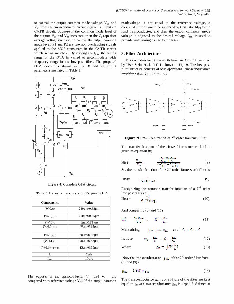
(IJCNS) International Journal of Computer and Network Security, Vol. 2, No. 5, May 2010
139
to control the output common mode voltage. Vop and Von from the transconductor circuit is given as inputs to CMFB circuit. Suppose if the common mode level of the outputs Vop and Von increases, then the Ca capacitor average voltage increases to control the output common mode level. P1 and P2 are two non overlapping signals applied to the MOS transistors in the CMFB circuit which act as switches. By varying the Itune, the tuning range of the OTA is varied to accommodate wide frequency range in the low pass filter. The proposed OTA circuit is shown in Fig. 8 and its circuit parameters are listed in Table 1.
M1 M2
M3
M4
M5M6
M7 M8
M15 M16
M13
M11 M12
Ib
Vi+ Vi-Vcm
Vb1
VDD
VSS
Vref
p1 p2 p1p2
p1p2 p2 p1
Itune
vop von
vop von
VCMF
VCMF
MF1 MF2
MF3 MF4
MF5 MF6
MF7 MF8
MF9
CS CSCa CaM14
M17
M9 M10
VB
Figure 8. Complete OTA circuit
Table 1 Circuit parameters of the Proposed OTA
The ouput’s of the transconductor Vop and Von are compared with reference voltage Vref. If the output common
modevoltage is not equal to the reference voltage, a corrected current would be mirrored by transistor MF9 to the load transconductor, and then the output common mode voltege is adjusted to the desired voltage. Itune is used to provide wide tuning trange to the filter.
3. Filter Architecture The second-order Butterworth low-pass Gm-C filter used by Uwe Stehr et al. [11] is shown in Fig. 9. The low pass filter structure consists of four operational transconductance amplifiers gm1, gm2, gm3 and gm4.
in+
in-
+
+ +
+
+
+gm1 gm2 gm3 gm4
+
out-
out+
2*C1
2*C1
2*C2
2*C2
Figure. 9 Gm- C realization of 2nd order low-pass Filter
The transfer function of the above filter structure [11] is given as equation (8)
H(s)= (8)
So, the transfer function of the 2nd order Butterworth filter is H(s)= (9) Recognizing the common transfer function of a 2nd order low-pass filter as H(s) = (10)
And comparing (8) and (10)
(11)
Maintaining and leads to (12)
Where (13)
Now the transconductance of the 2nd order filter from (8) and (9) is
(14)
The transconductance gm1, gm3 and gm4 of the filter are kept equal to gm and transconductance gm2 is kept 1.848 times of
Components Value
(W/L)1,2 250µm/0.35µm
(W/L)3,17 200µm/0.35µm
(W/L)4 1µm/0.35µm (W/L)5,6,7,8 40µm/0.35µm
(W/L)9,10 50µm/0.35µm
(W/L)11,12 20µm/0.35µm
(W/L)13,14,15,16 15µm/0.35µm
Ib 2µA Itune 10µA

(IJCNS) International Journal of Computer and Network Security, Vol. 2, No. 5, May 2010
140
gm to get the 2nd order Butterworth low pass filter response. This low pass filter is used in a direct conversion receiver to receive the mobile standards.
4. Simulation Results
4.1. Operational transconductance amplifier
Simulations of the proposed OTA and the filter are carried out with TSMC 0.35µm CMOS technology using H-Spice in synopsis. The implemented OTA and its open- loop AC frequency response are as shown in Fig. 10 (a) and (b) respectively.
Figure 10. (a) H-Spice Schematic of Implemented OTA circuit
Figure 10. (b) Frequency response of OTA
The step response of the OTA measures the slew rate of the filter to be 130 V/µs and is shown in Fig. 11.
Figure 11. Step transient response of the OTA
The variation in transconductance with reference to frequency is shown in Fig. 12. Simulation shows that the filter attains a transconductance value of 580µS.
Figure 12. Transconductance curve of the OTA
Figure 13. (a) Implemented 2nd order
4.2. 2nd order Butterworth low pass filter
The implemented circuit of 2nd order Butterworth low pass filter and its unity gain frequency response are shown in Fig. 13 (a) and (b) respectively. The maximum cut-off frequency of the filter is 3.9 MHz.

(IJCNS) International Journal of Computer and Network Security, Vol. 2, No. 5, May 2010
141
Figure 13. (b) Frequency response of the filter Butterworth Low Pass Filter circuit
A performance comparison of the 2nd order Butterworth low pass filter based on proposed OTA with other filters presented in literature recently is tabulated in Table 2.
Table 2 Performance Comparison Table
Parameter
Uwe
Stehr et
al. [11]
Wongnamk
um et al.
[10]
Tien-Yu
Lo et al.
[1]
Proposed
Work
CMOS- Tech
0.35-µm 0.35-µm 0.35-µm 0.35-µm
Supply voltage
2.5-V 1.5-V 2.5-V 1.1-V
MOS transistors
120 92 120 108
Power 500-mW 172-mW 1.9-mW 0.75-mW
THD
-35dB (0.6VPP
@ 2.5MHz)
-34dB (0.4VPP@ 2.5MHz)
-34dB (0.4VPP@ 2.5MHz)
-41dB (0.4VPP@ 2.5MHz)
HD3
-39dB
(0.6VPP
@
2.5MHz)
-41dB
(0.4VPP@
2.5MHz)
-50dB
(0.4VPP@
2.5MHz)
-47dB
(0.4VPP @2.5MH
z)
Slew rate of OTA
216 V/µs 185 V/µs 13 V/µs 130 V/µs
Gm 50µS 330µS 25µS 580µS
Tuning range
200KHz-2.5MHz
50KHz-5.7MHz
120KHz-2.25MHz
155KHz-
3.9.MHz
The filter proposed by Uwe Stehr et al. [11] utilizes conventional folded cascoded OTA for realizing the second order filter. This filter consumes large amount of power with poor noise performance though it has got a good slew rate. Also the OTA attains a very low transconductance value. In [10], a new class AB structure is introduced to increase the slewing behavior and transconductance value f OTA but with a high power consumption. In the transconductor proposed by Tien-Yu Lo et al.[1], a class AB structure utilizing FVF circuit act as a voltage to current converter along with a high linearity multiplier to minimize the third order harmonic distortion. This there forth reduces the power consumption of the filter but with poor the slew rate and transconductance value. So, in this paper an improved class AB structure which employs a cascoded FVF circuit to increase the slew rate and transconductance value of OTA is presented. The table illustrates that the filter with the proposed OTA outperforms the other filters in terms of low supply voltage, low power, reduced noise and wide tuning range.
5. Conclusion An improved operational transconductance amplifier is
proposed with a class AB pseudo differential structure with cascoded FVF. A 2nd order butter worth low pass filter used in a direct conversion receiver is implemented using 0.35µm, CMOS process with under 1.1V supply voltage. Simulation results show that the OTA attains a maximum transconductance value of 580µS as compared to other transconductor. Also the power consumption of the filter is 0.75mW at its maximum cutoff frequency. There forth the filter is suitable for low voltage, low power analog processing units.
References [1] Tien-Yu Lo and Chung-Chih Hung (2008), “Multi
mode Gm-C channel selections filter for mobile applications in 1-V supply voltage”, IEEE transactions on circuits and systems-II: express briefs, Vol.55.no.4, April.2008.
[2] J. Lim, Y. Jung and K. Jung, “A Wide-Band Active RC filter with a fast tuning scheme for wireless communication receivers”, Proc. IEEE CICC, Sep 2005 , pp. 637-640.
[3] A. C. M. de Queiroz and L. P. Caloba, “Passive symmetrical RLC filters suitable for active simulation”, IEEE International Symposium on Circuits and Systems, vol.3, Jun 1988, pp.2411-2414.
[4] B. Manai and P. Loumeau,“A Wide-band CMOS Switched Capacitor for UMTS direct conversion receiver”, Proc. IEEE MWSCAS, vol.1, 2001, pp.377-380.
[5] Y. Tsividis, M. Banu and J. Khoury, “Continuous-Time MOSFET-C filter in VLSI”, IEEE Trans. Circ. Syst.-II, Vol. CAS-33, No.2, 1886, pp.125–140.
[6] Sanchez-Sinencio, E, and Silva-Martinez J, “CMOS transconductance amplifiers, architectures and active filters: a tutorial,” IEEE Proc. On Circuits, Devices and Systems, vol.147, no.1, Feb 2000, pp.3-12.

(IJCNS) International Journal of Computer and Network Security, Vol. 2, No. 5, May 2010
142
[7] Ramon Gonzalez Carvaja, Jaime Ramirez-Angulol, Antonio J.Lopez-Martin, Antonio Torralba , Juan Antonio Gomez Galan, Alfonso Carlosena and Fernando Chavero, “The Flipped Voltage Follower : A Useful Cell for Low-Voltage Low-Power Circuit Design”, IEEE transactions on circuits and systems-I: Regular papers, Vol.52.no.7, July 2005.
[8] J. Ramirez-Angulo, S. G. Ivan Padilla, R. G. Carvajal, A. Torralba, M. Jimenez, F. Munoz and Antonio Lopez-Martin, “Comparison of Conventional and New Flipped Voltage Structures With Increased Input/output Signal Swing and Current Sourcing/Sinking Capabilities”, IEEE International Midwest Symposium on Circuits and Systems, Aug. 2005, pp. 1151-1154.
[9] Vlademir J.S Oliveira and Nobuo oki, “Low Voltage Four-Quadrant Current Multiplier: An improved Topology for n-well CMOS process”, IEEE, Trans. Design & Technology of Integrated Systems in Nanoscale Era, DTIS, Sept. 2007, pp.52-55.
[10] S. Wongnamkum and A. Thanachayanont , “New Class-AB Operational Transconductance Amplifier for High-Speed Switched-Capacitor Circuits”, IEEE International Symposium on Communications and Information Technology, vol.1, Oct 2004, pp. 531-535.
[11] Uwe Stehr, Frank Henkel, Lutz Dallige and Peter Waldow (2003), “A Fully Differential CMOS integrated 4th order reconfigurable GM-C Low Pass filter for mobile communication”, Proc. IEEE ICECS, Vol.1, Dec 2003, pp. 144-147.
Authors Profile
M.santhanalakshmi is currently working as Senior Lecturer in Electronics and Communication Department, PSG College of Technology, Coimbatore, India. She has about 9 years of teaching experience. Her research areas are Low power VLSI Design, Analog VLSI Design and Mixed Signal VLSI Design.
Dr.P.T.Vanathi is currently working as an Assistant Professor in Electronics and Communication department, PSG College of Technology, Coimbatore India. She has about 20 years of teaching experience. Her research areas are Speech Signal Processing, Image Processing and VLSI Design.
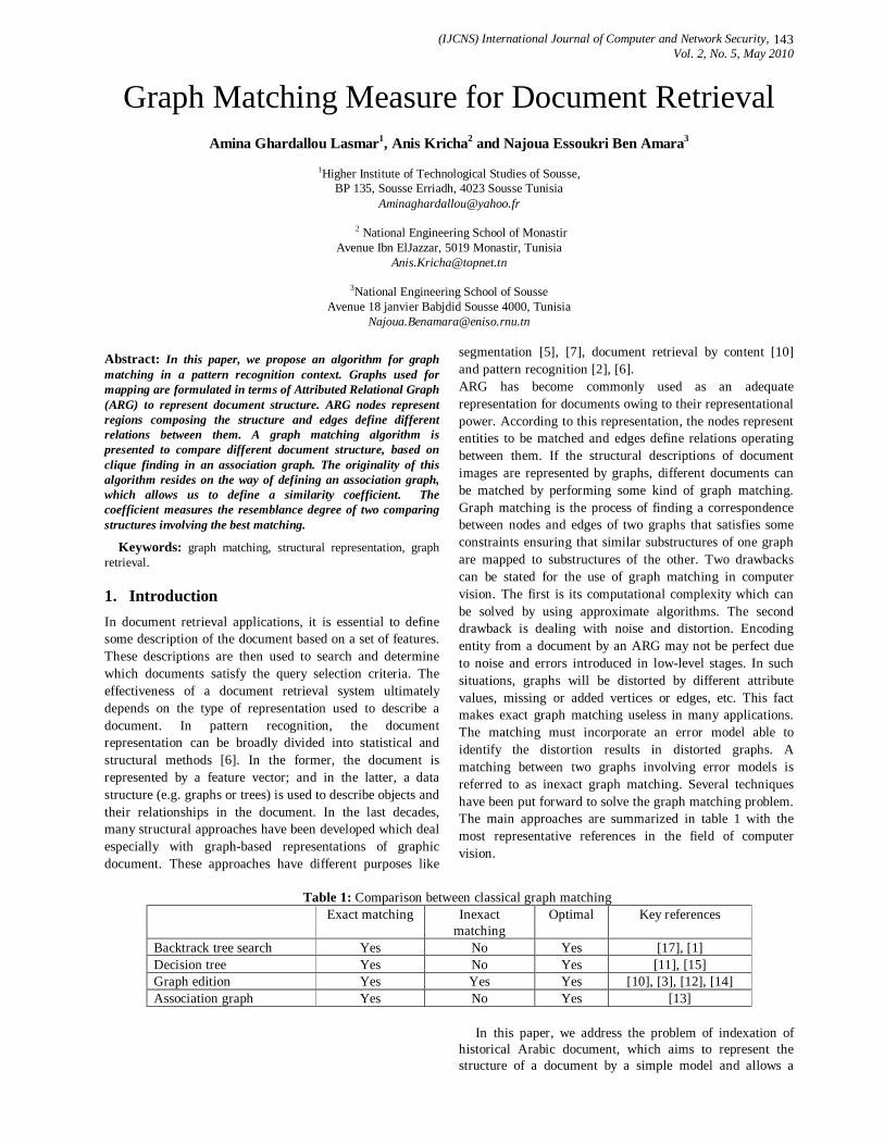
(IJCNS) International Journal of Computer and Network Security, Vol. 2, No. 5, May 2010
143
Graph Matching Measure for Document Retrieval
Amina Ghardallou Lasmar1, Anis Kricha2 and Najoua Essoukri Ben Amara3
1Higher Institute of Technological Studies of Sousse, BP 135, Sousse Erriadh, 4023 Sousse Tunisia
2 National Engineering School of Monastir Avenue Ibn ElJazzar, 5019 Monastir, Tunisia
3National Engineering School of Sousse Avenue 18 janvier Babjdid Sousse 4000, Tunisia
Abstract: In this paper, we propose an algorithm for graph matching in a pattern recognition context. Graphs used for mapping are formulated in terms of Attributed Relational Graph (ARG) to represent document structure. ARG nodes represent regions composing the structure and edges define different relations between them. A graph matching algorithm is presented to compare different document structure, based on clique finding in an association graph. The originality of this algorithm resides on the way of defining an association graph, which allows us to define a similarity coefficient. The coefficient measures the resemblance degree of two comparing structures involving the best matching.
Keywords: graph matching, structural representation, graph retrieval.
1. Introduction In document retrieval applications, it is essential to define some description of the document based on a set of features. These descriptions are then used to search and determine which documents satisfy the query selection criteria. The effectiveness of a document retrieval system ultimately depends on the type of representation used to describe a document. In pattern recognition, the document representation can be broadly divided into statistical and structural methods [6]. In the former, the document is represented by a feature vector; and in the latter, a data structure (e.g. graphs or trees) is used to describe objects and their relationships in the document. In the last decades, many structural approaches have been developed which deal especially with graph-based representations of graphic document. These approaches have different purposes like
segmentation [5], [7], document retrieval by content [10] and pattern recognition [2], [6]. ARG has become commonly used as an adequate representation for documents owing to their representational power. According to this representation, the nodes represent entities to be matched and edges define relations operating between them. If the structural descriptions of document images are represented by graphs, different documents can be matched by performing some kind of graph matching. Graph matching is the process of finding a correspondence between nodes and edges of two graphs that satisfies some constraints ensuring that similar substructures of one graph are mapped to substructures of the other. Two drawbacks can be stated for the use of graph matching in computer vision. The first is its computational complexity which can be solved by using approximate algorithms. The second drawback is dealing with noise and distortion. Encoding entity from a document by an ARG may not be perfect due to noise and errors introduced in low-level stages. In such situations, graphs will be distorted by different attribute values, missing or added vertices or edges, etc. This fact makes exact graph matching useless in many applications. The matching must incorporate an error model able to identify the distortion results in distorted graphs. A matching between two graphs involving error models is referred to as inexact graph matching. Several techniques have been put forward to solve the graph matching problem. The main approaches are summarized in table 1 with the most representative references in the field of computer vision.
Table 1: Comparison between classical graph matching
Exact matching Inexact matching
Optimal Key references
Backtrack tree search Yes No Yes [17], [1] Decision tree Yes No Yes [11], [15] Graph edition Yes Yes Yes [10], [3], [12], [14] Association graph Yes No Yes [13]
In this paper, we address the problem of indexation of historical Arabic document, which aims to represent the structure of a document by a simple model and allows a

(IJCNS) International Journal of Computer and Network Security, Vol. 2, No. 5, May 2010
144
further process like document or object retrieval. Therefore, we propose an ARG-based representation for the document physical structure. A graph matching method is then developed based on clique finding in an association graph to compare document structures. Results are then ranked according to coefficients which convey the degree of similarity between a query document and database documents. The remainder of the paper is organized as follows: In the next section, we propose the graph matching algorithm and we also introduce a similarity coefficient between two graphs. Experimentation is discussed in section 3. The final part concerns the conclusion and future works.
2. Proposed approach Even thought we are not interested in the segmentation step, we should consider error introduced by this step knowing that we operate with ancient documents, which includes much degradation. Thus, we will adapt an exact graph matching algorithm to our application to overcome distortion and errors introduced in precedent stages. The developed approach is based on a maximal clique finding in a modified association graph. First, we define a graph-based structure representation; the document structure is organized in an ARG whose nodes represent the different regions composing the document and the graph edges defining the spatial relations between these regions. The second step consists of constructing the association graph which is modified compared to the proposed definition in literature [8], [15] and adapted to our application. Finally, we define a similarity coefficient by examining the characteristics of the maximal clique in the AG.
2.1 Definition of the ARG ARG is a powerful means of giving structural
descriptions of visual patterns. Within an ARG, we can distinguish a syntactic part, made of the layout of unlabeled nodes and edges respectively identifying the structural primitive components of the pattern and their relations, and a semantic part consisting of the attributes associated to nodes and edges.
Formally an ARG graph is defined as a quadruple ),,,( EV LLEVG = , where V is the set of vertices,
VVE ×⊆ is the set of edges, and LV and LE are two labeling functions associating attributes to vertices and edges respectively. A document and its corresponding ARG structure are illustrated in Figure 1. In this figure, we denote the node labels (text or graphics), and near the connecting lines we denote edge labels (Upper; on the Right; Included; and Upper Right). We have excluded other spatial relations to avoid redundancy since the existence of a relation in a direction implies that it is complementary in the other one.
R
I
R
I1
I3
I2I2 I3
I1
(type: graphic)
(type: graphic)
(type:text)
R:in the right
I:included
Figure 1. A document image and the corresponding ARG
representation
2.2 A modified association graph for structure retrieval of the ARG
The proposed algorithm for graph matching is based on clique finding in an association graph, which is one of the most popular algorithms that can achieve an exact matching.
For the two graphs ),,1,1(1 11 EV LLEVG = and ),,2,2(2 22 EV LLEVG = , the association graph is a vertex labeled, undirected graph which can be created by the two step process [8], [15]:
1. For each correct vertex mapping from graph G1 to G2, insert a vertex in the association graph. This vertex is labeled with the vertex mapping between the vertices of G1 and G2.
2. For each pair of vertices va and wa in the association graph, insert the edge (va ,wa) if the vertices mapped from G1 have the same edge characteristics as the vertices mapped from G2.
Our approach is based on the construction of an association graph but with modification of the second step. We will insert edges not only when we retrieve all characteristics from vertices mapped from G1 and G2 but also when some characteristics are existing. In this way, the edges of the association graph will be level-headed with weights.
We note (I1, I2) tow vertices from G1and (J1, J2) from G2, where (I1, J1) and (I2, J2) present two correct mappings from graph G1 to G2. These weights are affected to AG edges as follows:
=⊂
≠
=
==
=
=
inverslyor
URJJLandRUIILifJJLIILif
JJLIILif
JJorIIifJIJIwv
EE
EE
EE
aa
)),(,),((),(),(2.0
),(),(1
)()(0)),(),,((),(
212211
212211
212211
2121
2211
32
(1)
In Figure 2, we illustrate an example of the way that we create an association graph from two graphs G1 (figure 2.a) and G2 (figure 2.b), candidates for comparison. Vertices of the AG are created from tow correspondent vertices from G1 and G2 (tow vertices are correspondent when they have similar attributes). Then AG edges are introduced between tow vertices with different weights (figure 2.c).
Let us remember that a clique is a complete sub-graph so that every pair of vertices is joined by an edge. Each clique within the association graph represents a set of vertices which have the same mutual relationships in G1 and G2; i.e., the cliques represent sub-graphs common to G1 and G2. In order to determine the number of possible common sub-graphs between two graphs, it is sufficient to examine the
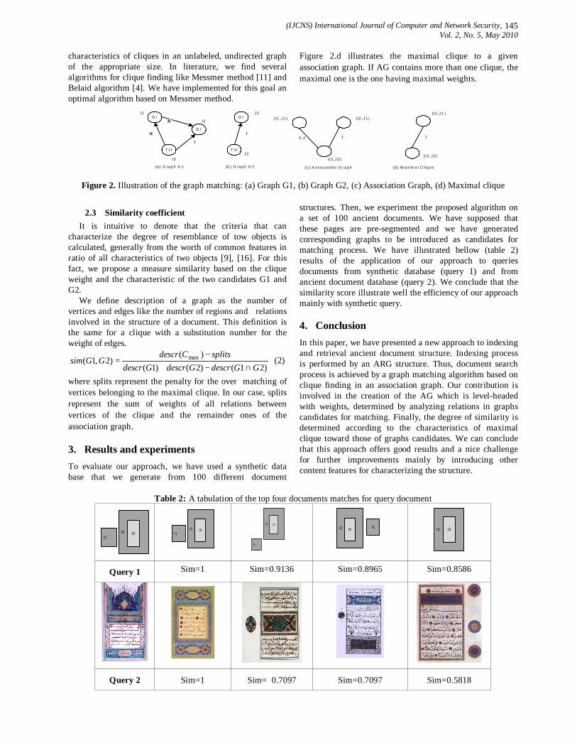
(IJCNS) International Journal of Computer and Network Security, Vol. 2, No. 5, May 2010
145
characteristics of cliques in an unlabeled, undirected graph of the appropriate size. In literature, we find several algorithms for clique finding like Messmer method [11] and Belaid algorithm [4]. We have implemented for this goal an optimal algorithm based on Messmer method.
Figure 2.d illustrates the maximal clique to a given association graph. If AG contains more than one clique, the maximal one is the one having maximal weights.
R
I
R
G r
T x t
G r
I1
I3
I2
T x t
G r
I
J 2
J 1(I2 ,J 1 )(I1 ,J 1 )
( I3 ,J 2 )
0 .2 1
(a ) G ra p h G 1 (b ) G ra p h G 2 (c ) A s s o c ia tio n G ra p h
1
(I2 ,J 1 )
(I3 ,J 2 )
(d ) M a x im a l C liq u e
Figure 2. Illustration of the graph matching: (a) Graph G1, (b) Graph G2, (c) Association Graph, (d) Maximal clique
2.3 Similarity coefficient It is intuitive to denote that the criteria that can
characterize the degree of resemblance of tow objects is calculated, generally from the worth of common features in ratio of all characteristics of two objects [9], [16]. For this fact, we propose a measure similarity based on the clique weight and the characteristic of the two candidates G1 and G2.
We define description of a graph as the number of vertices and edges like the number of regions and relations involved in the structure of a document. This definition is the same for a clique with a substitution number for the weight of edges.
)21()2()1()(
)2,1( max
GGdescrGdescrGdescrsplitsCdescr
GGsim∩−+
−= (2)
where splits represent the penalty for the over matching of vertices belonging to the maximal clique. In our case, splits represent the sum of weights of all relations between vertices of the clique and the remainder ones of the association graph.
3. Results and experiments To evaluate our approach, we have used a synthetic data base that we generate from 100 different document
structures. Then, we experiment the proposed algorithm on a set of 100 ancient documents. We have supposed that these pages are pre-segmented and we have generated corresponding graphs to be introduced as candidates for matching process. We have illustrated bellow (table 2) results of the application of our approach to queries documents from synthetic database (query 1) and from ancient document database (query 2). We conclude that the similarity score illustrate well the efficiency of our approach mainly with synthetic query.
4. Conclusion In this paper, we have presented a new approach to indexing and retrieval ancient document structure. Indexing process is performed by an ARG structure. Thus, document search process is achieved by a graph matching algorithm based on clique finding in an association graph. Our contribution is involved in the creation of the AG which is level-headed with weights, determined by analyzing relations in graphs candidates for matching. Finally, the degree of similarity is determined according to the characteristics of maximal clique toward those of graphs candidates. We can conclude that this approach offers good results and a nice challenge for further improvements mainly by introducing other content features for characterizing the structure.
Table 2: A tabulation of the top four documents matches for query document
I2 I3I1
I2 I3I1
I2 I3
I1
I2 I3 I1
I2 I3
Query 1 Sim=1 Sim=0.9136 Sim=0.8965 Sim=0.8586
Query 2 Sim=1 Sim= 0.7097 Sim=0.7097 Sim=0.5818

(IJCNS) International Journal of Computer and Network Security, Vol. 2, No. 5, May 2010
146
References [1] C. Ah-Soon. Analyse de plans architecturaux. Ph.D.
Thesis, Institut National Polytechnique de Lorraine, 1998.
[2] D. Arivault. Apport des graphes dans la reconnaissance non-contrainte de caractères manuscrits anciens. Ph.D Thesis, Université de Poitiers, 2006.
[3] R. Ambauen, S. Fisher, and H. Bunke. Graph edit distance with node splitting and merging, and its application to diatom identification. IAPR-TC15 Workshop on GbRPR, LNCS 2726, pp. 95-106, 2003.
[6] A. Belaïd, Y. Belaïd, “Reconnaissance des formes: Méthodes et applications,” InterEditions, 1992.
[7] F.P.G. Bergo, A.X. Falcão, P.A. Miranda, L.M. Rocha. “Automatic image segmentation by tree pruning,” Journal of Mathematical Imaging and Vision, 29(2-3), pp. 141-162, 2007.
[8] H. Bunke, S.Gunter, X.Jiang, “Towards bridging the gap between statistical and structural pattern recognition: Two new concepts in graph matching,” Advances in pattern recognition: ICAPR, Bresil, pp. 1-11, March 2001.
[9] P.F. Felzenszwalb, D.P. Huttenlocher, “Efficient graph-based image segmentation,” International Journal of Computer Vision, 59(2), pp. 167-181,2004.
[10] P. Heroux. “Contribution au problème de la rétro-conversion des documents structurés,” Ph.D.Thesis, Université de Rouen, 2001.
[11] D. Lin, An information theoric definition of Similarity. International Conférence on machines learning, pp. 296-304. Morgan Kaufmann, 1998.
[12] J. Lladós, “Symbol recognition by error-tolerant subgraph matching between region adjacency graphs,” IEEE Transactions on Pattern Analysis and Machine Intelligence, Vol. 23, No. 10, 2001.
[13] B.T Messmer. “Efficient graph matching algorithms for pre-processed model graphs,” Ph.D Thesis, Institut für Informatik und angewandte Mathematik, Université de Bern, Suisse, 1995.
[14] M. Neuhaus, H. Bunke. “Automatic learning of cost functions for graph edit distance,” Inform.Sci, 177 (1): pp 239-247, 2007.
[15] M.Pelillo, K.Siddiqi, S.W. Zucker. “Matching hierarchical structures using association graphs,” IEEE Trans. Pattern Analysis and Machine Intelligence, vol. 21, no. 11, pp.1105-1120, November 1999.
[16] K. Riesen, and H. Bunke. “Approximate graph edit distance computation by means of bipartite graph matching,” Image and Vision Computing, 27 (7), pp. 950-959, 2009.
[17] K. Shearer, H. Bunke, S. Venkatesh. “Video indexing and similarity retrieval by largest common subgraph detection using decision trees,” Pattern Recognition 34, pp.1075-1091, 2001.
[18] S.Sorlin. “Mesurer la similarité de graphes,” Ph. D Thesis, Université Claude Bernard Lyon I, 24 Novembre 2006.
[19] J.R. Ullman. “An algorithm for subgraph isomorphism,” Journal Association for Computer Machinery 23, pp.31-42, 1976.

(IJCNS) International Journal of Computer and Network Security, Vol. 2, No. 5, May 2010
147
Probability of Inquiry Interference in Bluetooth Discovery: Mathematical Analysis and Modeling
Khaled Morsi 1, Gao Qiang 2 and Xiong Huagang 3
1,2,3 Department of Electronic and Information Engineering
Beihang University (BUAA), Beijing, 100191, China 1 [email protected], 2 [email protected] and 3 [email protected]
Abstract: Bluetooth device discovery process involves nodes seeking to join neighboring piconets to enter inquiry substate. Nodes in a scatternet as well enter inquiry substate to discover other nodes within range. Inquiring nodes periodically send inquiry packets on a predetermined frequency partition of hop frequencies used by piconets. Intuitively, potential collisions will occur between inquiry packets and packets exchanged between piconet nodes during connection state, which lead to degraded network performance and longer discovery process. In this paper, we develop a mathematical model for interference caused by a single inquiring node, and extend the model to predict the severe interference levels due to multiple inquirers. We further validate our mathematical model through a simulation scenario. Analytical and simulation results proved that the probability of packets interfered and disrupted during inquiry procedure is periodic repeating every 3.16 sec and interference caused by a single inquiring node is about 1.25%. Results also revealed that five inquirers can disrupt 5.9% of network packets, and with increased number of inquiring nodes, the interference levels become more crucial approaching 35.3%.
Keywords: Bluetooth, Inquiry, Device Discovery, Interference
1. Introduction Device discovery is an essential process to establish and
maintain successful Bluetooth scatternets. This process is based on completing two phases; inquiry and paging. The inquiry phase is used to search and locate other Bluetooth devices within range. Nodes in a scatternet enter inquiry substate to discover other neighboring nodes. Nodes arriving in the vicinity as well enter inquiry substate seeking to join a pico- or scatternet. The inquiry procedure involves sending periodically inquiry packets on a predefined 32-frequency subset of 79 hop frequencies used by scatternet packets in normal connection state. Thus, interference is likely to occur between inquiry packets and connection state packets if they share the same frequency. Such interference will degrade network throughput, preclude device discovery process, and may result in undiscovered devices even within radio range.
The discovery process was discussed in previous studies. The authors in [1] developed an analytical model for time required by a master to discover one slave and proved that discovery time is affected by presence of multiple potential slaves. The work in [2] investigated optimization parameters needed to improve the performance of Bluetooth connection time. The authors in [5] analyzed the delay in discovery process for different situations and proposed means to decrease it. The proposed protocol in [6] does not separate inquiry and page phases to decrease interference, provide
faster links, and consume less power. In [7], the authors evaluated the factors affecting discovery time for multiple neighboring devices and introduced a modified inquiry scheme to accelerate discovery process. Through analysis and simulation, the authors in [8] proposed two ways to reduce delay in discovery process. The work in [9] analyzed the frequency-matching delay and proposed three schemes to speed up discovery procedure in Bluetooth.
The previous studies provided different mechanisms and new protocols to accelerate discovery process. However, the role of inquiry packets interference during discovery process was under estimated in most previous researches. We believe that reducing delay in discovery process, especially for multiple inquirers, depends mainly on avoiding such interference. This interference is not only generated when inquiry packets share same frequency with connection state packets. Both packets can also be indirectly disrupted if the header of the preceding packet is directly disrupted, even if they do not share the same frequency with inquiry packets. Thus, direct and indirect disruption will aggravate the inquiry interference problem.
The rest of this paper is organized as follows: In section 2, the Bluetooth inquiry substate is summarized. The Bluetooth connection state is illustrated in section 3. In section 4, the developed mathematical model for single inquiring node interference is presented. The extended model of multiple inquiring node interference is deduced in section 5. Final conclusions are given in section 6.
2. The Bluetooth Inquiry Substate A node enters the inquiry substate and acts as a master to
discover other potential slave nodes to form a piconet. In contrast, a node in the inquiry scan substate acts as a slave to be discovered by potential masters in the inquiry substate. Inquiring nodes use their resident CLK and General Inquiry Access Code (GIAC) address, (9E8B33)16, to generate a frequency hopping sequence among a predetermined 32-frequency subset of 79 Bluetooth frequencies [3]. The set of 32 inquiry frequencies is further segmented during inquiry into two 16-frequency trains, A and B.
An inquirer chooses A or B train for initial transmission and repeats this train for 256 times (256 x 625 usec x 16 = 2.56 sec), before switching to the other train [3]. The A-train or B-train is chosen when the parameter KOFFSET is set up to 24 or 8, respectively. The change of train is made by adding 16 to the current value of KOFFSET modulo 32. Three

(IJCNS) International Journal of Computer and Network Security, Vol. 2, No. 5, May 2010
148
changes have to be done within inquiry procedure length, which corresponds to 10.24 sec each 60 sec, as specified in [3]. As shown in Fig.1, the frequencies in these trains change over time such that each train always has 8 frequencies in the 54-69 index range (Lower Range) and 8 frequencies in the 70-79 and 1-6 index range (Upper Range).
Figure 1. Shifting and Selection of Inquiry Frequencies
An inquiring device transmits a 68-bit inquiry packet during an even time slot, when its two least significant clock bits are zero (CLK1,0=002). The frequency used is pseudo-randomly selected from lower range frequencies (FL) of the current train, A or B. Another upper range frequency (FU) is selected from the same train and used to transmit the second inquiry packet 312.5 usec later when (CLK1,0=012) as shown in Fig.2. During odd time slots, the inquirer listens for responses from neighboring devices in inquiry scan substate. Responses are transmitted 625 usec after an inquiry packet is received and transmitted on same frequencies, FL and FU [3]. The inquirer then selects new frequencies, FL and FU, and repeats the process, collecting data from as many neigh-boring nodes as possible during inquiry substate duration.
Figure 2. Bluetooth Inquiry, DH1, DH3, and DH5 Packets
3. The Bluetooth Connection State All members of a Bluetooth piconet hop together among
79 frequencies with a sequence that is a function of master's 28 bit free-running clock and first 28 bits of the master's 48 bit address [4]. The hop sequence cycle covers about 23.3 hours, spanning about 64 MHz of spectrum, spreading transmissions over 80% of the available 79 MHz band, and visiting all frequencies with equal probability [4]. The FH channel is based on Time Division Duplexing (TDD) using 625 usec time slots. Master packets are transmitted on even time slots and slaves respond on odd slots. Each time slot uses different hop frequency with hopping rate 1600 hops/s.
To increase data rate, and intuitively reduce hopping rate, multi-slot packets are defined to cover 1, 3, or 5 time slots, named DH1, DH3, or DH5, respectively. As shown in Fig.2, all packets contain a 72-bit Access Code to identify piconet and 54-bit Packet header containing the 3-bit slave address. Multi-slot packets will continue using same hop channel as being decided by first time slot, then, the system tunes back to the carrier frequency sequence as if only a single slot packet had been transmitted. Using this way, the hop frequency selection is not affected by packet lengths and all nodes can still hop synchronously.
During connection state, the instantaneous probability of a frequency being selected is based on 32-frequency partitions of the Bluetooth frequency band. The hop generator begins with a group of 32 frequencies that we call Master Frequencies Cycle (MFC) determined by master of piconet. The probability that a MFC is the same 32-frequency subset as that used by the inquiry substate is 1/79. The master transmits on a pseudo-randomly chosen frequency from MFC. The slave subsequently transmits on a frequency selected from a 32-frequency partition immediately right to the MFC which we term Slave Frequencies Cycle (SFC). Once each of the 32-frequencies in the MFC and SFC have been used exactly once (taking 64 time slots), both intervals shift right by 16 frequencies modulo 79 and frequency selection begins again as shown in Fig.3. The MFC/SFC shifts such that it uses all 79 MFC/SFC combinations before repeating a MFC/SFC such that the frequency selection is uniform across 79 frequencies. Within each MFC/SFC, the hopping sequence is pseudo-random, based on the master’s CLK and address [4].
Figure 3. MFC and SFC in Connection State
4. Single Inquiry Node Interference The time delay (DL) between inquiry packets and
piconets master and slave packets is significant, since it illustrates, not only difference between direct and indirect interference, but also it determines which packet (master,
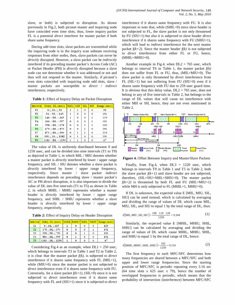
(IJCNS) International Journal of Computer and Network Security, Vol. 2, No. 5, May 2010
149
slave, or both) is subjected to disruption. As shown previously in Fig.2, both piconet master and inquiring node have coincided even time slots, thus, lower inquiry packet FL is a potential direct interferer for master packet if both share same frequency.
During odd time slots, slave packets are transmitted while the inquiring node is in the inquiry scan substate receiving responses from other nodes, then, slave packets can never be directly disrupted. However, a slave packet can be indirectly interfered if its preceding master packet’s Access Code (AC) or Packet Header (PH) is directly disrupted because a slave node can not determine whether it was addressed or not and thus will not respond to the master. Similarly, if piconet’s even slots coincided with inquiring node odd slots, slave / master packets are susceptible to direct / indirect interference, respectively.
Table 1: Effect of Inquiry Delay on Packet Disruption
The value of DL is uniformly distributed between 0 and
1250 usec, and can be divided into nine intervals (T1 to T9) as depicted in Table 1, in which MIL / MIU denotes whether a master packet is directly interfered by lower / upper range frequency, and SIL / SIU denotes whether a slave packet is directly interfered by lower / upper range frequency, respectively. Since master / slave packet indirect interference depends on preceding slave / master packet’s AC or PH direct disruption, it is also important to divide the value of DL into five intervals (T1 to T5) as shown in Table 2, in which MHIL / MHIU represents whether a master header is directly interfered by lower / upper range frequency, and SHIL / SHIU represents whether a slave header is directly interfered by lower / upper range frequency, respectively.
Table 2: Effect of Inquiry Delay on Header Disruption
Considering Fig.4 as an example, when DL1 = 250 usec,
which belongs to intervals T3 in Table 1 and T2 in Table 2, it is clear that the master packet f(k), is subjected to direct interference if it shares same frequency with FL (MIL=1), while (MIU=0) since the master packet is not subjected to direct interference even if it shares same frequency with FU. Conversely, for a slave packet f(k+1), (SIL=0) since it is not subjected to direct interference even if it shares same frequency with FL and (SIU=1) since it is subjected to direct
interference if it shares same frequency with FU. It is also important to note that, while (SHIL=0) since slave header is not subjected to FL, the slave packet is not only threatened by FU (SIU=1) but also it is subjected to slave header direct interference if it shares same frequency with FU (SHIU=1), which will lead to indirect interference for the next master packet f(k+ 2). Since the master header f(k) is not subjected to direct interference from either FL or FU, hence, (MHIL=MHIU=0).
Another example in Fig.4, when DL2 = 765 usec, which belongs to interval T6 in Table 1, the master packet f(k) does not suffer from FL or FU, thus, (MIL=MIU=0). The slave packet is only threatened by direct interference from FL (SIL=1) but not suffering from FU (SIU=0) even if it shares same frequency with FU due to 259 usec guard time. It is obvious that this delay value, DL2 = 765 usec, does not belong to any of five intervals in Table 2, but belongs to the range of DL values that will cause no interference with either MH or SH, hence, they are not even mentioned in Table 2.
Figure 4. Offset Between Inquiry and Master/Slave Packets
Finally, from Fig.4, when DL3 = 1220 usec, which belongs to intervals T9 in Table 1 and T5 in Table 2, both the slave packet f(k+1) and slave header are not subjected, therefore, (SIL=SIU=SHIL=SHIU=0). The master packet f(k+2) is threatened by both FL and FU (MIL=MIU=1) while MH is only subjected to FL (MHIL=1, MHIU=0).
If DL is unknown, the expected value E [MIL, MIU, SIL, SIU] can be used instead, which is calculated by averaging and dividing the range of values of DL which cause MIL, MIU, SIL, and SIU to equal 1 by the total range of DL, thus:
[ ] 344.01250
120119190,,, =++
=SIUSILMIUMILE (1)
Similarly, the expected value E [MHIL, MHIU, SHIL, SHIU] can be calculated by averaging and dividing the range of values of DL which cause MHIL, MHIU, SHIL, and SHIU to equal 1 by the total range of DL, hence:
[ ] 154.01250192,,, ==SHIUSHILMHIUMHILE (2)
The first frequency in each MFC/SFC determines how many frequencies are shared between a MFC/SFC and both upper and lower range frequencies. Since the starting position of MFC/SFC is periodic repeating every 3.16 sec (64 time slots x 625 usec x 79), hence the number of overlapped frequencies is periodic, which means that the probability of intersection (interference) between MFC/SFC
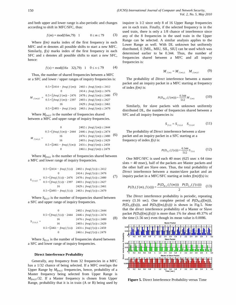
(IJCNS) International Journal of Computer and Network Security, Vol. 2, No. 5, May 2010
150
and both upper and lower range is also periodic and changes according to shift in MFC/SFC, thus:
1)79,16mod()( += mmf 790 ≤≤ m (3)
Where f(m) marks index of the first frequency in each MFC and m denotes all possible shifts to start a new MFC. Similarly, f(s) marks index of the first frequency in each SFC and s denotes all possible shifts to start a new SFC, hence:
1)79),3216mod(()( ++= ssf 790 ≤≤ s (4)
Thus, the number of shared frequencies between a MFC or a SFC and lower / upper ranges of inquiry frequencies is:
( )
( )( )
( )
−×
−×−×
−×
=
))((24935.016
2397))((5.02476))((5.0
0))((24145.0
),(
mffreq
mffreqmffreq
mffreq
M Umf
≤≤≤≤≤≤≤≤≤≤≤≤
2479))((24632461))((24292427))((24032480))((24782476))((24142412))((2402
mffreqmffreqmffreqmffreqmffreqmffreq
(5)
Where Mf(m),U is the number of frequencies shared between a MFC and upper range of inquiry frequencies.
( )
( )
−×
−×
=
0))((24615.0
1616
2444))((5.00
),(
mffreq
mffreq
M Lmf
≤≤≤≤≤≤≤≤≤≤≤≤
2479))((24612459))((24312429))((24032480))((24762474))((24462444))((2402
mffreqmffreqmffreqmffreqmffreqmffreq
(6)
Where Mf(m),L is the number of frequencies shared between a MFC and lower range of inquiry frequencies.
( )
( )( )
( )
−×
−×−×
−×
=
))((24935.016
2397))((5.02476))((5.0
0))((24145.0
),(
sffreq
sffreqsffreq
sffreq
S Usf
≤≤≤≤≤≤≤≤≤≤≤≤
2479))((24632461))((24292427))((24032480))((24782476))((24142412))((2402
sffreqsffreqsffreqsffreqsffreqsffreq
(7)
Where Sf(s),U is the number of frequencies shared between a SFC and upper range of inquiry frequencies.
( )
( )
−×
−×
=
0))((24615.0
1616
2444))((5.00
),(
sffreq
sffreq
S Lsf
≤≤≤≤≤≤≤≤≤≤≤≤
2479))((24612459))((24312429))((24032480))((24762474))((24462444))((2402
sffreqsffreqsffreqsffreqsffreqsffreq
(8)
Where Sf(s),L is the number of frequencies shared between a SFC and lower range of inquiry frequencies.
Direct Interference Probability
Generally, any frequency from 32 frequencies in a MFC has a 1/32 chance of being selected. If a MFC overlaps the Upper Range by Mf(m),U frequencies, hence, probability of a Master frequency being selected from Upper Range is Mf(m),U/32. If a Master frequency is chosen from Upper Range, probability that it is in train (A or B) being used by
inquirer is 1/2 since only 8 of 16 Upper Range frequencies are in each train. Finally, if the selected frequency is in the used train, there is only a 1/8 chance of interference since any of the 8 frequencies in the used train in the Upper Range can be selected. A similar analysis applies to the Lower Range as well. With DL unknown but uniformly distributed, E [MIL, MIU, SIL, SIU] can be used which was determined earlier to be 0.344. Thus, the number of frequencies shared between a MFC and all inquiry frequencies is:
UmfLmfmf MMM ),(),()( += (9)
The probability of Direct interference between a master packet and an inquiry packet in a MFC starting at frequency of index f(m) is:
)(, 512344.0)))((( mfIM MmfDP = (10)
Similarly, for slave packets with unknown uniformly distributed DL, the number of frequencies shared between a SFC and all inquiry frequencies is:
UsfLsfsf SSS ),(),()( += (11)
The probability of Direct interference between a slave packet and an inquiry packet in a SFC starting at a frequency of index f(s) is:
)(, 512344.0)))((( sfIS SsfDP = (12)
One MFC/SFC is used each 40 msec (625 usec x 64 time slots = 40 msec), half of the packets are Master packets and the other half are Slave ones. Thus, the total probability of Direct interference between a master/slave packet and an inquiry packet in a MFC/SFC starting at index f(m)/f(s) is:
2)))((()))(((
)))(),((( ,, sfDPmfDPsfmfDP ISIM
I+
= (13)
The Direct interference probability is periodic, repeating every (3.16 sec). One complete period of P(DM,I(f(m))), P(DS,I(f(s))), and P(DI(f(m),f(s))) is shown in Fig.5. Note that the direct interference probability of a Master or Slave packet P(DI(f(m),f(s))) is more than 1% for about 49.37% of the time (1.56 sec) even though its mean value is 0.0086.
0 0.2 0.4 0.6 0.8 1 1.2 1.4 1.6 1.8 2 2.2 2.4 2.6 2.8 3 3.20
0.01
0.02
Master Packet
0 0.2 0.4 0.6 0.8 1 1.2 1.4 1.6 1.8 2 2.2 2.4 2.6 2.8 3 3.20
0.01
0.02
Slave Packet
Dire
ct I
nter
fere
nce
Pro
babi
lity
0 0.2 0.4 0.6 0.8 1 1.2 1.4 1.6 1.8 2 2.2 2.4 2.6 2.8 3 3.20
0.005
0.01
Master or Slave Packet
Time ( sec )
Figure 5. Direct Interference Probability versus Time
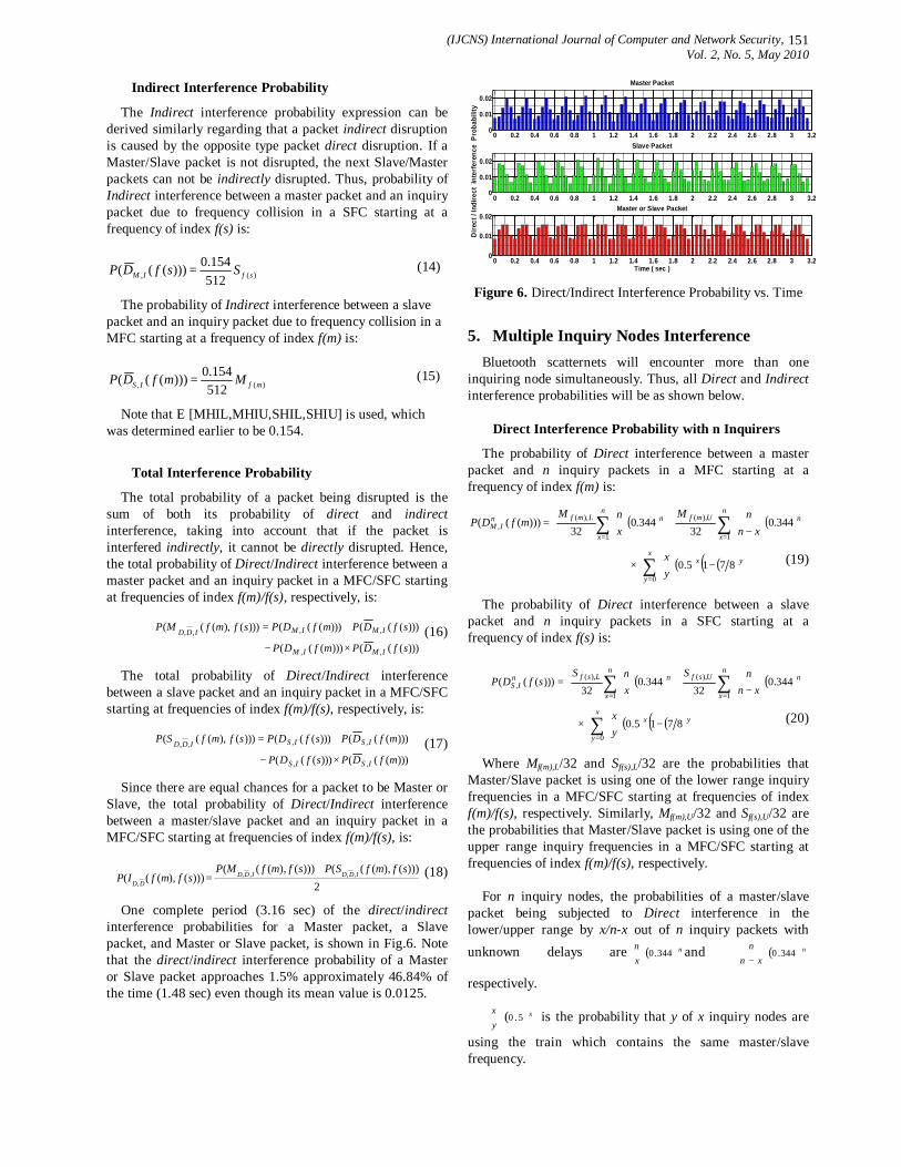
(IJCNS) International Journal of Computer and Network Security, Vol. 2, No. 5, May 2010
151
Indirect Interference Probability
The Indirect interference probability expression can be derived similarly regarding that a packet indirect disruption is caused by the opposite type packet direct disruption. If a Master/Slave packet is not disrupted, the next Slave/Master packets can not be indirectly disrupted. Thus, probability of Indirect interference between a master packet and an inquiry packet due to frequency collision in a SFC starting at a frequency of index f(s) is:
)(, 512154.0)))((( sfIM SsfDP = (14)
The probability of Indirect interference between a slave packet and an inquiry packet due to frequency collision in a MFC starting at a frequency of index f(m) is:
)(, 512154.0)))((( mfIS MmfDP = (15)
Note that E [MHIL,MHIU,SHIL,SHIU] is used, which was determined earlier to be 0.154.
Total Interference Probability
The total probability of a packet being disrupted is the sum of both its probability of direct and indirect interference, taking into account that if the packet is interfered indirectly, it cannot be directly disrupted. Hence, the total probability of Direct/Indirect interference between a master packet and an inquiry packet in a MFC/SFC starting at frequencies of index f(m)/f(s), respectively, is:
)))((()))(((
)))((()))((()))(),(((
,,
,,,,
sfDPmfDP
sfDPmfDPsfmfMP
IMIM
IMIMIDD
×−
+= (16)
The total probability of Direct/Indirect interference between a slave packet and an inquiry packet in a MFC/SFC starting at frequencies of index f(m)/f(s), respectively, is:
)))((()))(((
)))((()))((()))(),(((
,,
,,,,
mfDPsfDP
mfDPsfDPsfmfSP
ISIS
ISISIDD
×−
+= (17)
Since there are equal chances for a packet to be Master or Slave, the total probability of Direct/Indirect interference between a master/slave packet and an inquiry packet in a MFC/SFC starting at frequencies of index f(m)/f(s), is:
2)))(),((()))(),(((
)))(),((( ,,,,,
sfmfSPsfmfMPsfmfIP IDDIDD
DD
+= (18)
One complete period (3.16 sec) of the direct/indirect interference probabilities for a Master packet, a Slave packet, and Master or Slave packet, is shown in Fig.6. Note that the direct/indirect interference probability of a Master or Slave packet approaches 1.5% approximately 46.84% of the time (1.48 sec) even though its mean value is 0.0125.
0 0.2 0.4 0.6 0.8 1 1.2 1.4 1.6 1.8 2 2.2 2.4 2.6 2.8 3 3.20
0.01
0.02
Master Packet
0 0.2 0.4 0.6 0.8 1 1.2 1.4 1.6 1.8 2 2.2 2.4 2.6 2.8 3 3.20
0.01
0.02
Slave Packet
Dir
ect /
Indi
rect
Int
erfe
renc
e P
roba
bilit
y
0 0.2 0.4 0.6 0.8 1 1.2 1.4 1.6 1.8 2 2.2 2.4 2.6 2.8 3 3.20
0.01
0.02Master or Slave Packet
Time ( sec ) Figure 6. Direct/Indirect Interference Probability vs. Time
5. Multiple Inquiry Nodes Interference Bluetooth scatternets will encounter more than one
inquiring node simultaneously. Thus, all Direct and Indirect interference probabilities will be as shown below.
Direct Interference Probability with n Inquirers
The probability of Direct interference between a master packet and n inquiry packets in a MFC starting at a frequency of index f(m) is:
( ) ( )
−
+
= ∑∑
==
nn
x
Umfnn
x
LmfnIM xn
nMxnM
mfDP 344.032
344.032
)))(((1
),(
1
),(,
( ) ( )( )
−
× ∑
=
yxx
y yx
8715.00
(19)
The probability of Direct interference between a slave packet and n inquiry packets in a SFC starting at a frequency of index f(s) is:
( ) ( )
−
+
= ∑∑
==
nn
x
Usfnn
x
LsfnIS xn
nSxnS
sfDP 344.032
344.032
)))(((1
),(
1
),(,
( ) ( )( )
−
× ∑
=
yxx
y yx
8715.00
(20)
Where Mf(m),L/32 and Sf(s),L/32 are the probabilities that Master/Slave packet is using one of the lower range inquiry frequencies in a MFC/SFC starting at frequencies of index f(m)/f(s), respectively. Similarly, Mf(m),U/32 and Sf(s),U/32 are the probabilities that Master/Slave packet is using one of the upper range inquiry frequencies in a MFC/SFC starting at frequencies of index f(m)/f(s), respectively.
For n inquiry nodes, the probabilities of a master/slave packet being subjected to Direct interference in the lower/upper range by x/n-x out of n inquiry packets with unknown delays are ( )n
xn
344.0
and ( )n
xnn
344.0
−
respectively.
( )x
yx
5.0
is the probability that y of x inquiry nodes are
using the train which contains the same master/slave frequency.
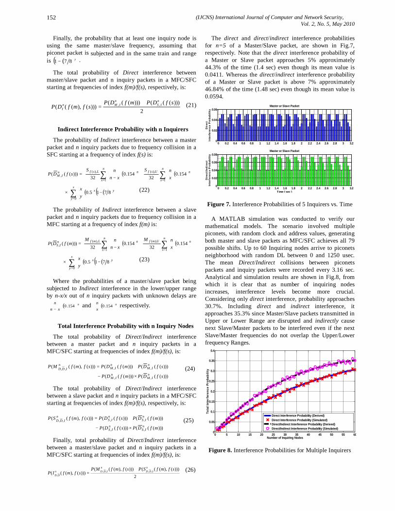
(IJCNS) International Journal of Computer and Network Security, Vol. 2, No. 5, May 2010
152
Finally, the probability that at least one inquiry node is using the same master/slave frequency, assuming that piconet packet is subjected and in the same train and range is ( )( )y871 − .
The total probability of Direct interference between master/slave packet and n inquiry packets in a MFC/SFC starting at frequencies of index f(m)/f(s), respectively, is:
2)))((()))(((
)))(),((( ,, sfDPmfDPsfmfDP
nIS
nIMn
I+
= (21)
Indirect Interference Probability with n Inquirers
The probability of Indirect interference between a master packet and n inquiry packets due to frequency collision in a SFC starting at a frequency of index f(s) is:
( ) ( )
+
−
= ∑∑
==
nn
x
Usfnn
x
LsfnIM x
nSxn
nSsfDP 154.0
32154.0
32)))(((
1
),(
1
),(,
( ) ( )( )
−
× ∑
=
yxx
y yx
8715.00
(22)
The probability of Indirect interference between a slave packet and n inquiry packets due to frequency collision in a MFC starting at a frequency of index f(m) is:
( ) ( )
+
−
= ∑∑
==
nn
x
Umfnn
x
LmfnIS x
nMxn
nMmfDP 154.0
32154.0
32)))(((
1
),(
1
),(,
( ) ( )( )
−
× ∑
=
yxx
y yx
8715.00
(23)
Where the probabilities of a master/slave packet being subjected to Indirect interference in the lower/upper range by n-x/x out of n inquiry packets with unknown delays are
( )n
xnn
154.0
−
and ( )n
xn
154.0
respectively.
Total Interference Probability with n Inquiry Nodes
The total probability of Direct/Indirect interference between a master packet and n inquiry packets in a MFC/SFC starting at frequencies of index f(m)/f(s), is:
)))((()))(((
)))((()))((()))(),(((
,,
,,,,
sfDPmfDP
sfDPmfDPsfmfMPn
IMn
IM
nIM
nIM
nIDD
×−
+= (24)
The total probability of Direct/Indirect interference between a slave packet and n inquiry packets in a MFC/SFC starting at frequencies of index f(m)/f(s), respectively, is:
)))((()))(((
)))((()))((()))(),(((
,,
,,,,
mfDPsfDP
mfDPsfDPsfmfSPn
ISn
IS
nIS
nIS
nIDD
×−
+= (25)
Finally, total probability of Direct/Indirect interference between a master/slave packet and n inquiry packets in a MFC/SFC starting at frequencies of index f(m)/f(s), is:
2)))(),((()))(),(((
)))(),((( ,,,,,
sfmfSPsfmfMPsfmfIP
nIDD
nIDDn
DD
+= (26)
The direct and direct/indirect interference probabilities for n=5 of a Master/Slave packet, are shown in Fig.7, respectively. Note that the direct interference probability of a Master or Slave packet approaches 5% approximately 44.3% of the time (1.4 sec) even though its mean value is 0.0411. Whereas the direct/indirect interference probability of a Master or Slave packet is above 7% approximately 46.84% of the time (1.48 sec) even though its mean value is 0.0594.
0 0.2 0.4 0.6 0.8 1 1.2 1.4 1.6 1.8 2 2.2 2.4 2.6 2.8 3 3.20
0.02
0.04
0.06Master or Slave Packet
Dir
ect
Inte
rfer
ence
Pro
babi
lity
0 0.2 0.4 0.6 0.8 1 1.2 1.4 1.6 1.8 2 2.2 2.4 2.6 2.8 3 3.20
0.02
0.04
0.06
0.08Master or Slave Packet
Dir
ect/I
ndir
ect
Inte
rfer
ence
Pro
babi
lity
Time ( sec )
Figure 7. Interference Probabilities of 5 Inquirers vs. Time
A MATLAB simulation was conducted to verify our mathematical models. The scenario involved multiple piconets, with random clock and address values, generating both master and slave packets as MFC/SFC achieves all 79 possible shifts. Up to 60 Inquiring nodes arrive to piconets neighborhood with random DL between 0 and 1250 usec. The mean Direct/Indirect collisions between piconets packets and inquiry packets were recorded every 3.16 sec. Analytical and simulation results are shown in Fig.8, from which it is clear that as number of inquiring nodes increases, interference levels become more crucial. Considering only direct interference, probability approaches 30.7%. Including direct and indirect interference, it approaches 35.3% since Master/Slave packets transmitted in Upper or Lower Range are disrupted and indirectly cause next Slave/Master packets to be interfered even if the next Slave/Master frequencies do not overlap the Upper/Lower frequency Ranges.
0 5 10 15 20 25 30 35 40 45 50 55 600
0.05
0.1
0.15
0.2
0.25
0.3
0.35
0.4
Number of Inquiring Nodes
Tota
l Int
erfe
renc
e Pr
obab
ility
Direct Interference Probability (Derived)Direct Interference Probability (Simulated)Direct/Indirect Interference Probability (Derived)Direct/Indirect Interference Probability (Simulated)
Figure 8. Interference Probabilities for Multiple Inquirers
(IJCNS) International Journal of Computer and Network Security, Vol. 2, No. 5, May 2010
153
6. Conclusions In this paper, we showed that during discovery process,
the potential collisions between both inquiry and scatternet packets in connection state are significant. Scatternet nodes and inquiring nodes will be affected by such interference that degrades network throughput and elongate discovery time. We further developed a mathematical model for interference probability caused by a single inquirer, and extended the model to predict the severe interference levels due to multiple inquiring nodes. Results revealed that interference probability is periodic, repeating every 3.16 sec over all possible MFC/SFC. The interference caused by a single inquirer is 1.25%. Five inquiring nodes result in interference probability of more than 7% for approximately 1.48 sec even though the mean probability of interference is only 0.059. However, as number of inquirers increase, the interference levels become more crucial. Considering only direct interference, results proved that probability reaches 30.7%. Including both direct and indirect interference, it approaches 35.3% since Master/Slave packets transmitted in Upper or Lower Range are always disrupted and indirectly cause the next Slave/Master packets to be interfered.
References [1] D. Chakraborty, G. Chakraborty, K. Naik, N. Shiratori,
“Analysis of the Bluetooth device discovery protocol”, Springer Wireless Networks Journal, February 2010, Vol. 16, pp.421-436.
[2] T. Thamrin, S. Sahib, “The Inquiry and Page Procedure in Bluetooth Connection,” IEEE Inter. Conf. SOCPAR09, Dec.2009, pp.218-222.
[3] www.bluetooth.com, “Bluetooth Specification v4.0”,Dec.17,2009
[4] M. Khaled, H. Xiong, Q. Gao, “Performance Estimation and Evaluation of Bluetooth Frequency Hopping Selection Kernel,” IEEE International Conference ICPCA09, Dec.2009, pp.461-466.
[5] D. Chakraborty, G. Chakraborty, S. Naik, N. Shiratori, “Discovery and Delay Analysis of Bluetooth Devices”, IEEE International Conference MDM06, May 2006, pp.113-117.
[6] S. Z. Kardos, A. Vidacs, “Performance of a new device discovery and link establishment protocol for Bluetooth”, IEEE International Conference GLOBECOM05, January 2006, Vol.6, pp.3522-3527.
[7] X. Zhang, G.F. Riley, “Evaluation and accelerating Bluetooth device discovery,” Radio and Wireless Symposium, Jan. 2006, pp.467-470.
[8] G. Chakraborty, K. Naik, D. Chakraborty, N. Shiratori, & D. Wei, , “Delay analysis and improvement of the device discovery protocol in Bluetooth”, IEEE Vehicular Tech. Conf., 2004, Los Angeles, USA.
[9] J. Jiang, B. Lin, & Y. Tseng, “Analysis of Bluetooth device discovery and some speedup mechanisms”, Journal of Institute of Electrical Engineering, 2004, 11(4), 301–310.
(IJCNS) International Journal of Computer and Network Security, Vol. 2, No. 5, May 2010
154
Color Image Segmentation Using Double Markov Random Field (DMRF) Model with Edge Penalty
Function
Sami M. Halawani1 , Ibrahim A. Albidewi2, M. M. Sani3 and M. Z. Khan3
1,2Faculty of Computing and Information Technology-Rabigh Campus King Abdulaziz University
Saudi Arabia [email protected], [email protected]
3Faculty of computer Science and Info. System
Jazan University K.S.A [email protected]
& Department of Computer Science and Engineering, IIET, Bareilly India
Abstract: In our paper color image segmentation using DMRF model with edge penalty function as image model and for color model using RGB and OHTA( )3,2,1 III color model. In our paper we are proposing Hybrid algorithm based on DMRF model and The image segmentation problem is formulated as a pixel labeling problem and the pixel labels are estimated using Maximum a Posterior(MAP) criterion. The MAP estimate of the labels are obtained by the proposed hybrid algorithm converges to the solution faster than that of Simulated Annealing(SA) algorithm. The DMRF with edge preserving attribute yields better segmentation result with local edge boundary. It is also found that Exponential function improved the result to some extend. The paper is divided in six section in second section we explain the model use for Hybrid Algorithm. Keywords: DMRF, MAP, RGB-Plane, Edge penalty function. 1. Introduction & Background Image segmentation is an important process in automated image analysis. In color image segmentation, choice of proper color model is one of the important factors for segmentation and different color models such as RGB, HSV, YIQ, OHTA ( )3,2,1 III , CIE (XYZ, Luv, Lab) are used to
represent different colors [1],[2][3]. Besides color model, image model does play a crucial role for color image segmentation. Stochastic models, particularly Markov Random Field (MRF) models, have been extensively used as the image model for image restoration and segmentation problems [4][5]. Often, in stochastic framework, the color image segmentation problem is formulated as a pixel labeling problem and the pixel labels are estimated using the Maximum a Posteriori (MAP) criterion[6][7]. By and large, the MAP estimates of the pixel labels are obtained using Simulated Annealing (SA) algorithm [11][8]. MRF model has also been successfully used as the image model while addressing the problem of color image segmentation in supervised and unsupervised framework [9]. Here we use, color image segmentation problem is formulated in stochastic framework. Markov Random Field model is used as the image model and RGB and OHTA model have been
used as the color models. we proposed a Double MRF (DMRF) model that takes case of intra-plane interactions as well as the inter-plane interactions[10]. These proposed models have been tested on different images and also the results obtained have been compared with the results obtained using only MRF. Both first order and second order models have also been studied. As expected, it has been observed that the use of OHTA model yielded better results than that of using RGB model We have used line process in the clique potential function and it has been found that although the line process could preserve well defined edges it failed to preserve loosely defined boundaries [11][12]. In order to preserve loosely defined boundaries, we have employed the edge penalty model proposed by Qiyao Yu et al [11][12]. Here, we have used RGB color models with MRF and DMRF models. Qiyao Yu et al [11][12] have used exponential edge penalty function preserve the weak edges together with strong edges. We have proposed the exponential edge penalty function in the DMRF model to preserve edge. Here also, the problem is formulated as a pixel labeling problem and the pixel label estimates are the MAP estimates.
2. Methodology Here we are proposing the model for our algorithms. The image segmentation problem is formulated as a pixel labeling problem. The labels are estimated using the MAP estimation criterion usually, the MAP estimates are obtained by Simulated Annealing (SA) algorithm. It is observed that SA algorithm is computationally involved and hence we have proposed a hybrid algorithm. Which is found to be faster than that of SA algorithm. The proposing models are as fallow. 2.1 Model 1 (Double Markov Random Field (DMRF) Model) The DMRF IS DEFINE AS In order color planes, the a prior

(IJCNS) International Journal of Computer and Network Security, Vol. 2, No. 5, May 2010
155
model takes case of intra-plane interactions and inter-plane interactions as well. This MRF model taking case of intra-plane and inter-plane interaction is called Double MRF (DMRF) model. Capturing salient spatial properties of an image leads to the development of image models. MRF theory provides a convenient and consistent way to model context dependent entities for eg. image pixel and correlated features. Through the MRF model takes into account the local spatial interactions, it has limitation in modeling natural scenes of distinct regions. In case of color models, it is known that there is a correlation among the color components of RGB model. In our formulation, we have de-correlated the color components and introduced an interaction process to improve the segmentation accuracy. We have employed inter-color plane interaction (OHTA ( 3,2,1 III ) color model) process which reinforces partial correlation among different color components. We assume all images to be defined on discrete on rectangular lattice .21 MM × Let Z denote the label process corresponding to the segmented image and z is a realization of the label process i.e. the segmented image. The observed image X is assumed to be a random field that is assumed to be the degraded version of the label process Z and this degradation process is assumed to be Gaussian process W. The label process Z in a given plane is assume to be MRF. The prior model takes care of inter as well as intra color plane interactions. The prior probability distribution of z is constructed with clique potential function corresponding to intra-color plane interaction, for example 1I and another clique potential function within inter plane interactions (for example between 1I and 2I ).The of inter color plane interaction are shows in Figure1.Thus X is a compound MRF. MRF model taking care of both inter as well as intra plane interactions. It known that if Z is assumed MRF, then the prior probability distribution P(Z=z) is Gibb’s distributed that can be expressed
as ( )θ|zZP = = ( )θ,'
1 zUe
Z
− , where ( )∑
−= z
zUeZ
θ,' is the
partition function,θ denotes the clique parameter vector, the exponential term U(z, θ ) is the energy function and is of the form
( ) ( )∑ ∈= Cc zcVzU θθ ,, with ( )θ,zcV being referred as the clique potential function. Since the inter-plane process is viewed to be MRF, we know
that ( ) ( ) ( )
∈∀≠== 1,,,,,1
,1,|2
,2
, IlkjilkI
lkzI
lkZI
jizI
jiZP
= ( ) ( ) ( )
∈≠== 1
,,,,,,1,
1,|2
,2
,I
jilkjilkI
lkzI
lkZI
jizI
jiZP η Where
1I and 2I denotes color planes respectively. In other words a
pixel in one plane (say for e.g 1I -plane) is assumed to have
interaction with pixel of 2I and 3I planes, the interaction process of each color plane is shown in Fig. 1(a). For the sake of illustration, the interaction of ( )thji, pixel in 2I plane with the neighboring pixels of 1I plane for a first order neighborhood system is also depicted in Fig. 1(b). The
observed image X which is assumed to be MRF is considered as a degraded version of the label process and hence consists of Z and W. The model parameter for both inter and intra color plane processes are selected on a trial and error basis. The weak membrane model is considered to the model intra as well as inter plane clique potential function. For example, the weak membrane model for inter-plane interaction process for two color components, ( 1I and 2I ) (as shown in Fig.1(b) ) can be expressed as
( )
−−+
−−=
21
1','2
','
21
',1'2
','1 I
jin
Iji
nI
jin
Iji
nzcV α +
+−+
+−
21
',1'2
','
21
1','2
','I
jin
Iji
nI
jin
Iji
n
Where α is the MRF field parameter. Superscripts 1I and
2I corresponds to
1I -plane and 2I -plane respectively. This
notation is depicted in Fig.1, where the intra plane and inter plane interaction are shown. The model parameter both Z and I processes are selected on an Ad hoc manner. The weak membrane model for intra plane as well as inter plane clique potential function.
Figure 1. (a) RGB Plane Interaction
Figure 1. (b) Interaction of one plane of R-plane with G-
plane 2.2 Model 2 (Segmantation in MRF-Map Framework Using Edge Penalty Function) Let Y denote the observed data (i.e the original image) and X the desired segmentation. The following optimality criterion is used
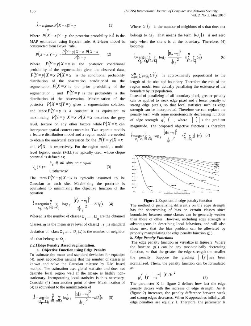
(IJCNS) International Journal of Computer and Network Security, Vol. 2, No. 5, May 2010
156
( )yYxXPx
x === |maxarg) (1)
Where ( )yYxXP == | the posterior probability is x) is the MAP estimation using Baysian rule. A 2-layer model is constructed from Bayes’ rule.
( ) ( ) ( )( )yYP
xXPxXyYPyYxXP
====
===|
| (2)
Where ( )xXyYP == | is the posterior conditional probability of the segmentation given the observed data,
( ) ( )xXPxXyYP === | is the conditional probability distribution of the observation conditioned on the segmentation, ( )xXP = is the prior probability of the
segmentation , and ( )yYP = is the probability is the distribution of the observation. Maximization of the posterior ( )yYxXP == | gives a segmentation solution,
and since ( )yYP = is a constant it is equivalent to
maximizing ( ) ( )xXPxXyYP === | describes the grey
level, texture or any other factors while ( )xXP = can incorporate spatial context constraint. Two separate models a feature distribution model and a region model are needed to obtain the analytical expression for the ( )xXyYP == |
and ( )xXP = respectively. For the region model, a multi-level logistic model (MLL) is typically used, whose clique potential is defined as;
=)(XcV
otherwise
equalconsitesallifc
:0
:β (3)
The term ( )xXyYP == | is typically assumed to be Gaussian at each site. Maximizing the posterior is equivalent to minimizing the objective function of the equation
( )[ ]
( )( )∑
=∑ −
−+=
Ω=ΩΩ
n
isiU
i
isYix
isn 1 22
2logminarg
,....1
βσ
µσ) (4)
Whereη is the number of classesn
ΩΩ ,.....,1
are the obtained
Classes, iµ is the mean grey level of class iΩ , iσ is standard
deviation of class iΩ ,and )(sU i is the number of neighbor
of s that belongs to iΩ .
2.2.1Edge Penalty Based Segmentation. a. Objective Function using Edge Penalty
To estimate the mean and standard deviation for equation (4), most approaches assume that the number of classes is known and solve the Gaussian mixture by E-M based method. The estimation uses global statistics and does not describe local region well if the image is highly non-stationary. Incorporating local statistics is thus necessary. Consider (4) from another point of view. Maximization of (4) is equivalent to the minimization of
( ) ( )[ ]( )
( )
∑=
∑Ω=
−−
+ΩΩ
=n
i ssiU
i
isYi
nx
1 1
'22
2log
,...1minarg β
σ
µσ) (5)
Where ( )siU ' is the number of neighbors of s that does not
belongs to iΩ . That means the term ( )siU 'β is not zero
only when the site s is at the boundary. Therefore, (4) becomes
( )[ ]
( )( )∑
=∑Ω=
∑=
∑Ω=
+−
+ΩΩ
=
n
i is
n
i issiU
i
isYi
nx
1 1'
22
2log
,....1minarg β
σ
µσ) (6)
( )∑ = ∑ Ω=ni is siU1
' is approximately proportional to the
length of the obtained boundary. Therefore the role of the region model term actually penalizing the existence of the boundary by its population. Instead of penalizing of all boundary pixel, greater penalty can be applied to weak edge pixel and a lesser penalty to strong edge pixels, so that local statistics such as edge strength can be incorporated. Therefore we can replace the penalty term with some monotonically decreasing function of edge strength ( )( ).∇g , where ( ).∇ is the gradient magnitude. The proposed objective function is therefore
( )[ ]( )
( )( )( )∑=
∑ ∑ ∑ ∇+−
+=Ω= = Ω=ΩΩ
n
is
n
i isn isYg
i
isYix
1 22
2logminarg
1,....1β
σ
µσ) (7)
Figure 2.Exponential edge penalty function
The method of penalizing differently on the edge strength has the shortcoming of bias on certain classes since boundaries between some classes can be generally weaker than those of other. However, including edge strength is advantageous in describing local behaviors, and will also show next that the bias problem can be alleviated by properly manipulating the edge penalty function g(.). b. Edge Penalty Functions The edge penalty function as visualize in figure 2. Where the function g(.) can be any monotonically decreasing function, so that the greater the edge strength the smaller the penalty. Suppose the grading ( )Y∇ has been normalized. Them, the penalty function can be formulated as:
( )( ) ( )( )2/KYeYg
∇−=∇ (8)
The parameter K in figure 2 defines how fast the edge penalty decays with the increase of edge strength. As K (figure 2) increases, the penalty difference between weak and strong edges decreases. When K approaches infinity, all edge penalties are equally 1. Therefore, the parameter K
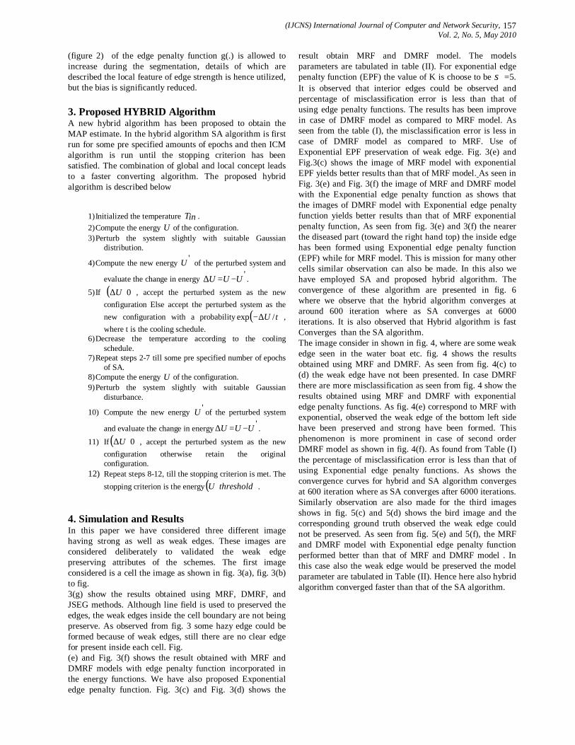
(IJCNS) International Journal of Computer and Network Security, Vol. 2, No. 5, May 2010
157
(figure 2) of the edge penalty function g(.) is allowed to increase during the segmentation, details of which are described the local feature of edge strength is hence utilized, but the bias is significantly reduced. 3. Proposed HYBRID Algorithm A new hybrid algorithm has been proposed to obtain the MAP estimate. In the hybrid algorithm SA algorithm is first run for some pre specified amounts of epochs and then ICM algorithm is run until the stopping criterion has been satisfied. The combination of global and local concept leads to a faster converting algorithm. The proposed hybrid algorithm is described below
1) Initialized the temperature inT . 2) Compute the energy U of the configuration. 3) Perturb the system slightly with suitable Gaussian
distribution.
4) Compute the new energy 'U of the perturbed system and
evaluate the change in energy 'UUU −=∆ . 5) If ( )0⟨∆U , accept the perturbed system as the new
configuration Else accept the perturbed system as the new configuration with a probability ( )tU /exp ∆− , where t is the cooling schedule.
6) Decrease the temperature according to the cooling schedule.
7) Repeat steps 2-7 till some pre specified number of epochs of SA.
8) Compute the energy U of the configuration. 9) Perturb the system slightly with suitable Gaussian
disturbance.
10) Compute the new energy 'U of the perturbed system
and evaluate the change in energy 'UUU −=∆ . 11) If ( )0⟨∆U , accept the perturbed system as the new
configuration otherwise retain the original configuration.
12) Repeat steps 8-12, till the stopping criterion is met. The stopping criterion is the energy( )thresholdU ⟨ .
4. Simulation and Results In this paper we have considered three different image having strong as well as weak edges. These images are considered deliberately to validated the weak edge preserving attributes of the schemes. The first image considered is a cell the image as shown in fig. 3(a), fig. 3(b) to fig. 3(g) show the results obtained using MRF, DMRF, and JSEG methods. Although line field is used to preserved the edges, the weak edges inside the cell boundary are not being preserve. As observed from fig. 3 some hazy edge could be formed because of weak edges, still there are no clear edge for present inside each cell. Fig. (e) and Fig. 3(f) shows the result obtained with MRF and DMRF models with edge penalty function incorporated in the energy functions. We have also proposed Exponential edge penalty function. Fig. 3(c) and Fig. 3(d) shows the
result obtain MRF and DMRF model. The models parameters are tabulated in table (II). For exponential edge penalty function (EPF) the value of K is choose to be σ =5. It is observed that interior edges could be observed and percentage of misclassification error is less than that of using edge penalty functions. The results has been improve in case of DMRF model as compared to MRF model. As seen from the table (I), the misclassification error is less in case of DMRF model as compared to MRF. Use of Exponential EPF preservation of weak edge. Fig. 3(e) and Fig.3(c) shows the image of MRF model with exponential EPF yields better results than that of MRF model. As seen in Fig. 3(e) and Fig. 3(f) the image of MRF and DMRF model with the Exponential edge penalty function as shows that the images of DMRF model with Exponential edge penalty function yields better results than that of MRF exponential penalty function, As seen from fig. 3(e) and 3(f) the nearer the diseased part (toward the right hand top) the inside edge has been formed using Exponential edge penalty function (EPF) while for MRF model. This is mission for many other cells similar observation can also be made. In this also we have employed SA and proposed hybrid algorithm. The convergence of these algorithm are presented in fig. 6 where we observe that the hybrid algorithm converges at around 600 iteration where as SA converges at 6000 iterations. It is also observed that Hybrid algorithm is fast Converges than the SA algorithm. The image consider in shown in fig. 4, where are some weak edge seen in the water boat etc. fig. 4 shows the results obtained using MRF and DMRF. As seen from fig. 4(c) to (d) the weak edge have not been presented. In case DMRF there are more misclassification as seen from fig. 4 show the results obtained using MRF and DMRF with exponential edge penalty functions. As fig. 4(e) correspond to MRF with exponential, observed the weak edge of the bottom left side have been preserved and strong have been formed. This phenomenon is more prominent in case of second order DMRF model as shown in fig. 4(f). As found from Table (I) the percentage of misclassification error is less than that of using Exponential edge penalty functions. As shows the convergence curves for hybrid and SA algorithm converges at 600 iteration where as SA converges after 6000 iterations. Similarly observation are also made for the third images shows in fig. 5(c) and 5(d) shows the bird image and the corresponding ground truth observed the weak edge could not be preserved. As seen from fig. 5(e) and 5(f), the MRF and DMRF model with Exponential edge penalty function performed better than that of MRF and DMRF model . In this case also the weak edge would be preserved the model parameter are tabulated in Table (II). Hence here also hybrid algorithm converged faster than that of the SA algorithm.
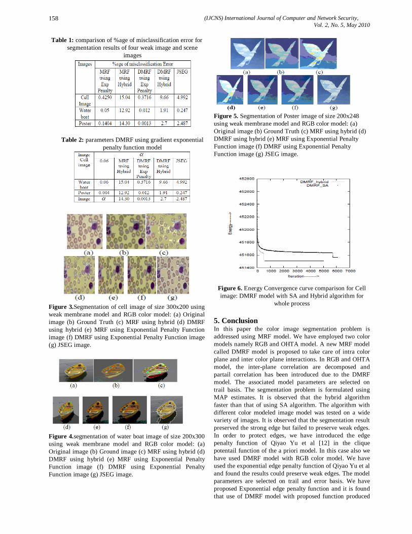
(IJCNS) International Journal of Computer and Network Security, Vol. 2, No. 5, May 2010
158
Table 1: comparison of %age of misclassification error for segmentation results of four weak image and scene
images
Table 2: parameters DMRF using gradient exponential penalty function model
Figure 3.Segmentation of cell image of size 300x200 using weak membrane model and RGB color model: (a) Original image (b) Ground Truth (c) MRF using hybrid (d) DMRF using hybrid (e) MRF using Exponential Penalty Function image (f) DMRF using Exponential Penalty Function image (g) JSEG image.
Figure 4.segmentation of water boat image of size 200x300 using weak membrane model and RGB color model: (a) Original image (b) Ground image (c) MRF using hybrid (d) DMRF using hybrid (e) MRF using Exponential Penalty Function image (f) DMRF using Exponential Penalty Function image (g) JSEG image.
Figure 5. Segmentation of Poster image of size 200x248 using weak membrane model and RGB color model: (a) Original image (b) Ground Truth (c) MRF using hybrid (d) DMRF using hybrid (e) MRF using Exponential Penalty Function image (f) DMRF using Exponential Penalty Function image (g) JSEG image.
Figure 6. Energy Convergence curve comparison for Cell image: DMRF model with SA and Hybrid algorithm for
whole process 5. Conclusion In this paper the color image segmentation problem is addressed using MRF model. We have employed two color models namely RGB and OHTA model. A new MRF model called DMRF model is proposed to take care of intra color plane and inter color plane interactions. In RGB and OHTA model, the inter-plane correlation are decomposed and partail correlation has been introduced due to the DMRF model. The associated model parameters are selected on trail basis. The segmentation problem is formulated using MAP estimates. It is observed that the hybrid algorithm faster than that of using SA algorithm. The algorithm with different color modeled image model was tested on a wide variety of images. It is observed that the segmentation result preserved the strong edge but failed to preserve weak edges. In order to protect edges, we have introduced the edge penalty function of Qiyao Yu et al [12] in the clique potentail function of the a priori model. In this case also we have used DMRF model with RGB color model. We have used the exponential edge penalty function of Qiyao Yu et al and found the results could preserve weak edges. The model parameters are selected on trail and error basis. We have proposed Exponential edge penalty function and it is found that use of DMRF model with proposed function produced

(IJCNS) International Journal of Computer and Network Security, Vol. 2, No. 5, May 2010
159
better result than that of using DMRF model. We have employed hybrid and SA to obtain segmentation and hybrid algorithm converges faster than that of SA algorithm. Current work focuses estimation of model parameters and devising an unsupervised scheme. References [1] L. Lucchese and S.K. Mitra , “Color Image
Segmentation: A state of the art survey”, Proc of the Indian National Science Academy , volume 67, No. 2, (feb 2006): pp. 207-221
[2] Chen H.D., Jiang X.H., Sun Y., and Wang J., “Color Image Segmentation: advances and prospects,”Pattern Recognition, volume 34, 2000: pp.2259-2281.
[3] Gonzalez R.C. and Woods R.E. Digital image processing. Singapore: Pearson Education, 2001.
[4] Stan Z. Li, “Markov Field Modeling in Image analysis,” Japan: Springer, 2001.
[5] Geman. S and Geman D, “ Stochastic relaxation, Gibbs distributions, and the Bayesian
Restoration of images, “IEEE Transaction on Pattern Analysis and Machine Intelligence, volume 6, No. 6, November 1984: 721-741.
[6] Kato. Z Pong. T. and Lee J.C., “Color Image Segmentation and Parameter Estimation in a Markovian framework,” Pattern Recognition Letters, volume 22, No. 2, 2001: pp. 309-321.
[7] Kato. Z. and Pong. T. , “ A Markov Random Field Image Segmentation model using Combined Color and Texture Feature, “ Proceeding of International Conference on Computer Analysis of Image and Patterns. (September 2001): pp. 547-554.
[8] Kirkpatrick S., Gelatt C.D., and Vecchi M.P., “Optimization by Simulated Annealing,” Science, volume 220, No. 4598, 1983: pp. 671-679.
[9] Panjawani D.K. and healey G., “Markov Random Field Models for Unsupervised Segmentation of Texture Color Images.” IEEE Transaction on Pattern Analysis and Machine Intelligence, volume 17, No.10,(October 1995): pp. 939-954.
[10] P.K. Nanda, MRF Model Learning and its Application to Image Restoration and Segmentation PhD Dessertation, Electrical Engg. Department, IIT Bombay 1995
[11] Qiyao Yu, David A . Clausi, “IRGS: Image Segmentation Using Edge Penalties and Region Growing,” IEEE Transaction on Pattern Analysis and Machine Intelligence PAMI.
[12] Qiyao Yu, David A. Clausi, “Combination Local and Global Feature for Image Segmentation Using Iterative
Classification and Region Merging,” Proc of the Second Canadian Conference on Computer and Robot Vision volume 1(May 2005):pp.579-586.
(IJCNS) International Journal of Computer and Network Security, Vol. 2, No. 5, May 2010
160
Performance Evaluation of a Reed-Solomon Encoded Multi-user Direct Sequence Code Division
Multiple Access (DS-CDMA) Communication System
Nargis Parvin, Farhana Enam, Shaikh Enayet Ullah and Md. Saifur Rahman
Department of Information and Communication Engineering
Rajshahi University, Rajshahi-6205, Bangladesh. Abstract: This paper incorporates a comprehensive study on the performance evaluation of a Reed-Solomon encoded multi-user Direct Sequence Code Division Multiple Access (DS-CDMA) communication system in terms of Bit Error Rate (BER). The DS-CDMA system under present study employing uncorrelated spreading codes has incorporated BPSK digital modulation over an Additive White Gaussian Noise (AWGN) and other fading (Rayleigh and Rician) channels. Computer simulation results on BER demonstrate that the Reed-Solomon encoded multi-user DS-CDMA system outperforms in retrieving the transmitted messages of the individual senders .The system is highly effective to combat inherent interferences under Rayleigh and Rician fading channels. It is anticipated from the study that the performance of the communication system degrades with the lowering of the Signal-to-Noise Ratio (SNR).
Keywords: Direct Sequence Code Division Multiple Access
(DS- CDMA), Signal-to-Noise Ratio (SNR), Additive White Gaussian Noise (AWGN), Fading channels.
1. Introduction Direct Sequence Code Division Multiple Access (DS-CDMA) is one of the most prominent air-interface techniques in today’s wireless communication systems [1]. In a DS-CDMA system all users transmit in the same bandwidth simultaneously [2]. This transmission technique is a multiple access communication scheme in which each user is assigned a unique spreading code for modulating the transmitted symbols. Thus, a receiver with knowledge about the code of the intended transmitter can select the desired signal. A DS-CDMA communication system receiver has generally three main obstacles to overcome such as Multiple Access Interference (MAI) from other users, Inter-symbol Interference (ISI) due to a multipath channel and additive noise at the receiver. In a DS-CDMA system, the transmitter multiplies each user’s signal by a pseudo-random spreading sequence [3], [4]. In fact, user’s spreading codes are designed to be orthogonal (or quasi-orthogonal). However, due to channel properties like multipath propagation, orthogonality cannot be maintained at the receiver and the signals interfere with each other. In practical CDMA systems the spreading codes among the users are not perfectly orthogonal. Thus, a CDMA channel with randomly
and independently chosen spreading sequences accurately models the situation where pseudo-noise sequences span many symbol periods [5]. Direct Sequence Code Division Multiple Access (DS-CDMA) has already been established as a strong candidate for third-generation mobile and personal communication systems. Now a days, the most prominent applications of the CDMA are in mobile communication systems like cdmaOne (IS-95), UMTS or cdma2000. To apply CDMA in a mobile radio environment, specific additional methods are required to be implemented in all these systems. Methods such as power control and soft handover have to be applied to control the interference by other users and to be able to separate the users by their respective codes [6], [7].
2. System Description We assume that a multi-user Direct Sequence Code Division Multiple Access (DS-CDMA) communication system depicted in Figure 1 utilizes a Reed-Solomon channel coding scheme. In transmitting section of the present Reed-Solomon encoded DS-CDMA system, a typically named b source information bits of rate rb are grouped and mapped to one of the M= 2b information symbols. The information symbols with rate of rs= rb/ log2M ks/s (ksymbols/s) enter a (n, k, t) Reed–Solomon encoder operating in GF (M) with n, k, t=[n-k]/2. The output of the Reed–Solomon encoded symbols is of rate rsc= rs/rc, where, rc= k/n. The coded symbols are fed into symbol to binary converter and its output are then converted into bipolar NRZ format and subsequently fed into BPSK digital modulator. The digitally modulated signals are then multiplied with the generated pseudo-random noise for each user. The pseudo randomly noise contaminated modulated signals for user1 and user2 are then added up and passed through AWGN or fading channel. The channel output is then multiplied with the generated pseudo-random noise and demodulated. The demodulated signal for each user is processed through integrator. The integrated output is sent up to the decision-making device and eventually, the information bits

(IJCNS) International Journal of Computer and Network Security, Vol. 2, No. 5, May 2010
161
transmitted for each user are recovered [8], [9].
Figure 1. Block diagram of a Reed- Solomon Encoded Multi-user DS-CDMA system
The present study has been made on the consideration of model parameters shown in Table 1.
Table 1: parameters used in system simulation No. of bits used for synthetic data 1,912 Bit rate 1,000 bits/sec Energy per bit (eb) 0.5 Chip rate 10,000
chips/sec Channel Coding Reed-
Solomon Doppler Frequency 100 HZ Carrier frequency 5 MHz K-factor used in Rician fading 10 SNR 0 to10 dB
3. Results and Discussion Figure 2 shows a segment of original binary bit stream of individual user. The noise contaminated received signals for a typical SNR value of 5 dB in Rayleigh fading channel and its amplitude spectrum are illustrated in Figure 3 and
Figure 4 respectively. In Figure 4, it is quite evident that the amplitude of the signal is maximum around the frequency of 100 KHz. Figure 5 demonstrates the simulation results for uncoded multi-user DS-CDMA communication system under an AWGN channel. It is observable that its value approaches zero for a SNR value of 5 dB. In Figure 6, the BER simulated graphs under AWGN and Rayleigh fading channels are illustrated for user 1 and user 2.
Figure 2. A segment of original binary bit stream of individual user.
Figure 3. Received Signal with Additive White Gaussian
noise and Rayleigh fading effects incorporated.
Figure 4. Amplitude Spectrum of noise contaminated
received signal with added Rayleigh fading channel effect.
Binary data for user #1
Binary data for user #2
Direct sequence generator for user # 2
Retrieved data Reed-Solomon Decoder
Mapping into bipolar NRZ 1 to +1 0 to –1
BPSK modulator
RF carrier
Mapping into bipolar NRZ: 1 to +1 0 to –1
BPSK modulator
RF carrier
Direct sequence generator
for user # 2
Direct sequence generator for user # 1
BPSK Demodulator
BPSK Demodulator
Integrator
Sampling
Detection Device
Retrieved data
d
Integrator
Sampling
Detection Device
Reed-Solomon Encoder
Reed-Solomon Encoder
Reed-Solomon Decoder
RF carrier
RF carrier
AWGN/ Fading channel
Direct sequence generator for user #1

(IJCNS) International Journal of Computer and Network Security, Vol. 2, No. 5, May 2010
162
Figure 5. BER Performance of the uncoded multiuser DS-
CDMA communication system under AWGN channel.
Figure 6. BER Performance of the uncoded multiuser DS-
CDMA communication system under AWGN and Rayleigh fading channels
In Figure 7, the BER simulated graphs under AWGN and Rician fading channels are illustrated for user 1 and user 2. The bit error rate approaches zero at 3 dB and 4 dB for user 1 and user 2 respectively. The BER performance of multi-user DS-CDMA communication system on deployment with Reed-Solomon channel coding scheme under AWGN channel is shown in Figure 8. It is observable that the bit error rate approaches zero at 2 dB for both user 1 and user 2 viz. the system provides better performance as compared to uncoded situation.
Figure 7. BER Performance of the uncoded multi-user DS-CDMA communication system under AWGN and
Rician fading channels.
Figure 8. BER Performance of the Reed- Solomon
encoded multi-user DS-CDMA communication system under AWGN channel.
The BER performance of Reed-Solomon encoded multi-user DS-CDMA communication system under AWGN and Rayleigh fading channels is shown in Figure 9. Similarly, the system performance under AWGN and Rician fading channels is shown in Figure 10. In comparison of BER values for a typical SNR value of zero dB (Figure 9 and Figure 10), it is found that the bit error rate for Rayleigh and Rician fading channels are 0.0455 and 0.011 respectively. This is due to the fact that in case of Rician fading, the direct component of transmitted signal is more prominent as compared to multipath components and as a consequence of which the bit error rate is reduced with enhancement of system performance.
Figure 9. BER Performance of the Reed- Solomon
encoded multi-user DS-CDMA communication system under AWGN and Rayleigh fading channels.
Figure 10. BER Performance of the Reed- Solomon
encoded multi-user DS-CDMA communication system under AWGN and Rician fading channels.
(IJCNS) International Journal of Computer and Network Security, Vol. 2, No. 5, May 2010
163
4. Conclusions In our present study, we have studied the performance of a multi-user Direct Sequence Code Division Multiple Access (DS-CDMA) communication system adopting the Reed-Solomon channel coding and BPSK digital modulation scheme. A range of system performance results highlight the impact of a simplified digital modulation technique and different uncorrelated spreading codes. In the context of system performance, it can be concluded that the implementation of BPSK digital modulation technique in Reed-Solomon channel encoded multi-user Direct Sequence Code Division Multiple Access (DS-CDMA) communication system provides satisfactory performance in retrieving the transmitted messages of the individual users.
References [1] W. C. Y. Lee, “Overview of cellular CDMA,” IEEE
Transactions on Vehicular Technology, vol. 40, no. 2, pp. 291–302, 1991.
[2] P. Jung, P. W. Baeir, and A. Steil, “Advantages of CDMA and spread spectrum techniques over FDMA and TDMA in cellular mobile radio applications,” IEEE Transactions on Vehicular Technology, vol. 42, no. 3, pp. 357–364, 1993.
[3] R L. Pickholtz, D. L. Schilling, and L. B. Milstein, “Theory of spread-spectrum communications” A tutorial, IEEE Transactions on Communications, vol. 30, no. 5, pp. 855–884, 1982.
[4] R. L. Pickholtz, L. B. Milstein, and D. L. Schilling, “Spread spectrum for mobile communications,” IEEE Transactions on Vehicular Technology, vol. 40, no. 2, pp. 313–322, 1991.
[5] F. C. M. Lau and C. K. Tse, “Chaos-Based Digital Communication Systems: Operating Principles, Analysis Methods, and Performance Evaluation,” First edition, Springer, 2003.
[6] K.S. Gilhousen et al., “On the Capacity of a Cellular CDMA System”, IEEE Trans. Vehic. Technol., Vol. 40, no. 2, pp. 303–312, 1991.
[7] M.G. Jansen and R. Prasad, “Capacity, Throughput, and Delay Analysis of a Cellular DS CDMA System With Imperfect Power Control and Imperfect Sectorization”, IEEE Trans. Vehic. Technol., Vol. 44, no. 1, pp. 67–75, 1995.
[8] A.C. Iossifides and F-N. Pavlidou, ‘’ Performance of RS-Coded DS/CDMA Micro cellular Systems with
M-ary orthogonal Signaling,” Wireless Personal Communications 10: pp. 33–52, Netherlands, 1998.
[9] Rappaport, S.Theodore,“Wireless Communications,” Principle and Practice, Second Edition, Pearson Educatiob (Singapore) Pte., Ltd.,New Delhi,India, 2004.
Authors Profile Nargis Parvin received the B.Sc. and M.Sc. degree in Information and Communication Engineering from University of Rajshahi, Bangladesh. Farhana Enam received the B.Sc. and M.Sc. degree in Computer Science from University of Rajshahi, Bangladesh.. She is currently working as Assistant Professor of the dept. of Information and Communication Engineering, University of Rajshahi, Bangladesh. Shaikh Enayet Ullah received the B.Sc. and M.Sc. degree in Applied Physics from University of Rajshahi, Bangladesh.. He has completed his PhD from Jahangirnagor University, Bangladesh. He is currently working as a Professor and Chairman of the dept. of Information and Communication Engineering, University of Rajshahi, Bangladesh. Saifur Rahman received the B.Sc. and M.Sc. degree in Information and Communication Engineering from University of Rajshahi, Bangladesh.
(IJCNS) International Journal of Computer and Network Security, Vol. 2, No. 5, May 2010
164
Phase Information Extraction of Atrial Fibrillation Using Wavelets
1 V.Bindhu 2G.Ranganathan 3Dr.R.Rangarajan
1Asst.Professor, PPG Institute of Technology, Affiliated to Anna University Coimbatore, India 2Associate Professor, RVS School Of Engineering and Technology, Affiliated to Anna University Coimbatore, India
3Principal, Sri Ramakrishna Engineering College, Affiliated to Anna University Coimbatore, India
[email protected], [email protected] Abstract: A novel method for characterization of phase information in atrial fibrillation (AF) is presented. The method decomposes atrial activity into fundamental and harmonic components, dividing each component into short blocks for which the amplitudes, frequencies, and phases are estimated. The phase delays between the fundamental and each of the harmonics, here referred to as harmonic phase relationships, are used as features of f-wave morphology. The estimated waves are clustered into typical morphologic patterns. The performance of the method is illustrated by simulated signals, ECG signals recorded from 36 patients with organized AF, and an ECG signal recorded during drug loading with flecainide. The results show that the method can distinguish a wide variety of f-wave morphologies, and that typical morphologies can be established for further analysis of AF. Keywords: Atrial Fibrillation (AF), Electrocardiogram (ECG), Reverse biorthogonal wavelets, waveform characterization. 1. Introduction
ATRIAL fibrillation (AF) is a heterogeneous
disease considered to be the resulting end state of several mechanisms. Initiation of AF typically requires both a triggering event and an arrhythmia-prone anatomical substrate [1]–[3]. Suggested triggers include abnormal activity of the autonomic nervous system and rapidly firing foci located in the pulmonary veins. The arrhythmia-prone substrate may result from, e.g., impaired impulse propagation, changes in tissue structure, or alternations in atrial electrical properties induced by the arrhythmia itself. AF has mainly been viewed as an acquired disorder related to structural heart disease in patients with other cardiovascular problems, including coronary artery and mistral valve diseases and hypertension [4]; however, AF is now recognized to also have a heritable component [5]. Characterization of AF based on ECG recordings calls for separation of atrial and ventricular activity. Several approaches to such separation have been suggested based on, e.g., principal component analysis [6], [7], independent component analysis [8], and patio temporal modeling [9], [10]. The most important aspect of AF pattern analysis has, so far, been to determine the fibrillatory rate. This rate has potential value for monitoring spontaneous and autonomic maneuver-induced changes in atrial electrophysiology, monitoring and prediction of anti arrhythmic drug responses
as well as for prediction of atrial defibrillation thresholds and AF recurrence following cardio version . AF with slower rates seems more likely to terminate spontaneously or to respond to anti-arrhythmic drug therapy whereas faster rates are more often found in persistent and drug- and cardio version-refractory AF . Recently, methods for characterizing temporal AF dynamics have been developed for studying mechanisms and treatment strategies. Using time-domain methods, the properties of f-waves have been investigated in terms of the plane of best fit and the spatial phase properties of different ECG planes . Time–frequency analysis, combined with frequency alignment of an adaptively updated spectral profile, has been used to track variations in AF frequency and f-wave morphology. Morphologic characterization was based on the harmonics pattern, expressed as the exponential decay of the harmonics’ magnitude. The significance of AF harmonics has been paid little attention in the literature, one reason being that spectral analysis is almost invariably based on longer segments (> 30 s). As a Consequence, each segment contains large temporal variations in AF frequency that smears the harmonics. The aforementioned time–frequency analysis is particularly well suited to handle such variations in AF frequency as spectral alignment is performed, facilitating the detection and characterization of harmonics [23]. Several important questions related to the interpretation of AF patterns in the ECG remain unanswered, including how the patterns can be used to determine disease state and predict treatment outcome in individual patients. Other questions relate to the meaning of f-wave morphology in terms of intra-atrial activation patterns and to signal-based identification of AF subgroups. The use of AF frequency alone does not answer these questions. In this paper, we introduce a novel approach to f-wave factorization based on signal phase analysis. The method has a two-stage structure in which the atrial activity is first translated into compact sets of features, which are then clustered so that the typical waveform patterns can be discerned. The morphologic parameters of the present method offer information complementary to the atrial rate and are not intended as a replacement to rate. The paper is outlined as follows: the method is presented in Section II, simulated and ECG signals in Section III, the results are presented in Section IV, and a discussion of the method and its performance is found in Section V.
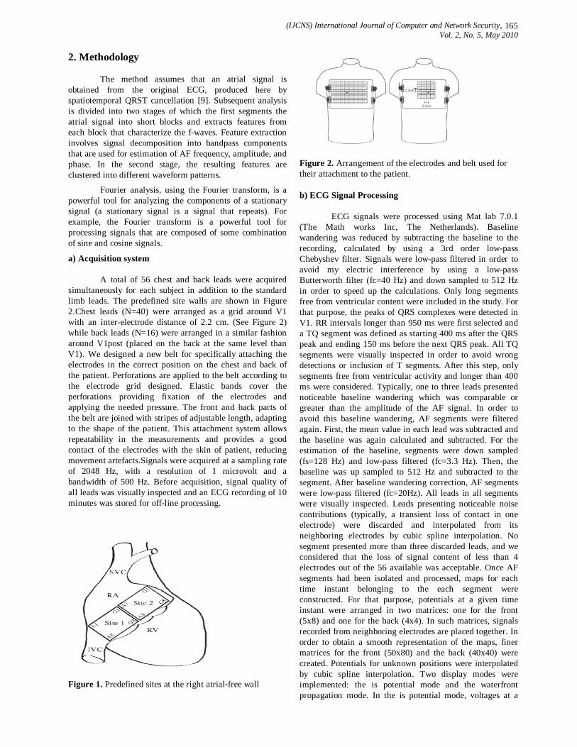
(IJCNS) International Journal of Computer and Network Security, Vol. 2, No. 5, May 2010
165
2. Methodology
The method assumes that an atrial signal is obtained from the original ECG, produced here by spatiotemporal QRST cancellation [9]. Subsequent analysis is divided into two stages of which the first segments the atrial signal into short blocks and extracts features from each block that characterize the f-waves. Feature extraction involves signal decomposition into bandpass components that are used for estimation of AF frequency, amplitude, and phase. In the second stage, the resulting features are clustered into different waveform patterns.
Fourier analysis, using the Fourier transform, is a powerful tool for analyzing the components of a stationary signal (a stationary signal is a signal that repeats). For example, the Fourier transform is a powerful tool for processing signals that are composed of some combination of sine and cosine signals.
a) Acquisition system
A total of 56 chest and back leads were acquired simultaneously for each subject in addition to the standard limb leads. The predefined site walls are shown in Figure 2.Chest leads (N=40) were arranged as a grid around V1 with an inter-electrode distance of 2.2 cm. (See Figure 2) while back leads (N=16) were arranged in a similar fashion around V1post (placed on the back at the same level than V1). We designed a new belt for specifically attaching the electrodes in the correct position on the chest and back of the patient. Perforations are applied to the belt according to the electrode grid designed. Elastic bands cover the perforations providing fixation of the electrodes and applying the needed pressure. The front and back parts of the belt are joined with stripes of adjustable length, adapting to the shape of the patient. This attachment system allows repeatability in the measurements and provides a good contact of the electrodes with the skin of patient, reducing movement artefacts.Signals were acquired at a sampling rate of 2048 Hz, with a resolution of 1 microvolt and a bandwidth of 500 Hz. Before acquisition, signal quality of all leads was visually inspected and an ECG recording of 10 minutes was stored for off-line processing.
Figure 1. Predefined sites at the right atrial-free wall
Figure 2. Arrangement of the electrodes and belt used for their attachment to the patient. b) ECG Signal Processing
ECG signals were processed using Mat lab 7.0.1 (The Math works Inc, The Netherlands). Baseline wandering was reduced by subtracting the baseline to the recording, calculated by using a 3rd order low-pass Chebyshev filter. Signals were low-pass filtered in order to avoid my electric interference by using a low-pass Butterworth filter (fc=40 Hz) and down sampled to 512 Hz in order to speed up the calculations. Only long segments free from ventricular content were included in the study. For that purpose, the peaks of QRS complexes were detected in V1. RR intervals longer than 950 ms were first selected and a TQ segment was defined as starting 400 ms after the QRS peak and ending 150 ms before the next QRS peak. All TQ segments were visually inspected in order to avoid wrong detections or inclusion of T segments. After this step, only segments free from ventricular activity and longer than 400 ms were considered. Typically, one to three leads presented noticeable baseline wandering which was comparable or greater than the amplitude of the AF signal. In order to avoid this baseline wandering, AF segments were filtered again. First, the mean value in each lead was subtracted and the baseline was again calculated and subtracted. For the estimation of the baseline, segments were down sampled (fs=128 Hz) and low-pass filtered (fc=3.3 Hz). Then, the baseline was up sampled to 512 Hz and subtracted to the segment. After baseline wandering correction, AF segments were low-pass filtered (fc=20Hz). All leads in all segments were visually inspected. Leads presenting noticeable noise contributions (typically, a transient loss of contact in one electrode) were discarded and interpolated from its neighboring electrodes by cubic spline interpolation. No segment presented more than three discarded leads, and we considered that the loss of signal content of less than 4 electrodes out of the 56 available was acceptable. Once AF segments had been isolated and processed, maps for each time instant belonging to the each segment were constructed. For that purpose, potentials at a given time instant were arranged in two matrices: one for the front (5x8) and one for the back (4x4). In such matrices, signals recorded from neighboring electrodes are placed together. In order to obtain a smooth representation of the maps, finer matrices for the front (50x80) and the back (40x40) were created. Potentials for unknown positions were interpolated by cubic spline interpolation. Two display modes were implemented: the is potential mode and the waterfront propagation mode. In the is potential mode, voltages at a

(IJCNS) International Journal of Computer and Network Security, Vol. 2, No. 5, May 2010
166
given time instant were represented according to a color scale. Videos of each AF segment were generated. In the wave front propagation mode, only lines connecting points on the surface with a voltage equals to zero were represented. This display mode allows the visualization of both the polarization and re polarization wave fronts depending on the time interval selected. The succession of wave fronts is represented using a color scale according to the time instant in which each wave front appears. We used a method as previously reported [16]. After removal of a 50-Hz disturbance component emanating from power supplies, and after subtraction of the mean signal level of all recordings, data reduction by means of low-pass filtering, and resembling at rate of 100 Hz, experimental data from the 78 electrode array were arranged in impulse response matrices of dimensions the number being the number of data points in each recording between two consecutive heart beats. Subsequent impulse response analysis and simulation of the resulting state-space realization were applied as described in next section. 3. Results and Discussion
Maps were generated for all the segments considered in the study and visually inspected. Single or multiple simultaneous wave fronts, wave breakages and disorganized electrical activity could be observed. Figure 2 shows some selected wave front propagation maps representative patterns observed. In panel 1a, a succession of wave fronts from patient 3 is observed. A single wave front can be observed in both panels 1a and 1b. In panel 1a wave fronts are mostly parallel to each other. Panel 1b shows the next succession of wave fronts, which differ from panel 1a.Panels 2a and 2b show two consecutive depolarization waves from patient 3 which present a similar pattern. Surface wave fronts rotate along a similar axis in both panels. The same pattern was observed in the consecutive wave fronts appearing in the same segment (total=5).Panel 3 shows two consecutive depolarization waves from patient 5.
Depolarization wave shown in panel a is first
shown in the leftmost part on bottom of the grid and spreads towards the center and top until it gets blocked. A second depolarization wave starts in the uppermost part on the right of the grid and propagates towards the bottom and the left until it gets blocked in roughly the same position where the previous wave arrived. It can be observed that one wave front is blocked by the previous propagation contributing to a chaotic propagation. Panels 4a and 4b show depolarization waves in patient 6. Multiple waves arise at the same time, propagate and then disappear in an uncoordinated fashion.
By analyzing the 10-minute recording of each
patient, we observed that the wave front propagation patterns were, to some extent, repeatable. Patient 3 showed clear wave fronts with similar patterns in most segments analyzed. Patients 1, 5 and 6 showed a completely unstable pattern with multiple simultaneous activation wave fronts that changed widely even in short time intervals. Patients 2 and 4 presented an intermediate degree of repeatability, with one or two simultaneous propagation wave fronts that could
both differ greatly or slightly from one activation to another. By application of the state-space realization algorithm to every heart beat with a period of approximately 1 s and 175 ms during atrial fibrillation, it was possible to reproduce the electro gram impulse response which, in turn, makes possible a quantitative comparison as to the variation and complexity of a set of consecutive heart beats. The wavelet decomposition of scddvbrk signal is shown in Figure 3.
Figure 3. wavelet decomposition of scddvbrk signal
Relative prediction error versus model order and
the singular value sequences indicate a model order to be relevant for the SR and the atrial pacing, whereas a model order is relevant for atrial fibrillation. As for the temporal and channel-dependent autocovariances and cross covariance of data and residuals, it is apparent that atrial fibrillation data exhibit other temporal covariance than data of SR and of artificial atrial pacing data. The phase curve extraction of standard signals like scddvbrk, freqdbrk and cuspamax provides useful information in the atrial fibrillation. The phase curve extraction using freqdbrk signal is shown in Figure 4.
Figure 4. Phase curve extraction using freqdbrk Signal
The phase curve extraction using cuspamax signal
is shown in Figure 4.

(IJCNS) International Journal of Computer and Network Security, Vol. 2, No. 5, May 2010
167
Figure 5. Phase curve extraction using freqdbrk Signal
Modeling: Generally, the purposes of theoretical models are to pinpoint deficiencies in our knowledge about a system and to predict properties of the system which otherwise should not have emerged. In our case we have studied heart surface properties of impulse propagation as the impulse response to natural and artificial pacing. Thus, the nonlinear modeling needed to reproduce the impulse generation and refractory tissue properties is not included. As for all behaviorist models, the models obtained here provide no final or definite answer as to the underlying physiological mechanisms. Although the linear properties of the underlying physiological processes might be challenged, the system identification provides linear approximate models of finite and low complexity and good prediction accuracy. As for methodological extensions, the realization theory applied here lends itself to modeling by linear partial differential equations by using the spatial information available in the electro gram data.
The linear models obtained for electro grams of SR,
atrial pacing, and atrial fibrillation have been validated by means of approximation notions and (preliminary) extensions of statistical validation properties including cross validation on data sets not used for system parameter estimation. The phase curve extraction used above are applicable to the ECG signal. The raw ECG data is denoised and applied to phase curve extraction using reverse bi-orthogonal wavelet is shown below.
0 500 1000 1500-1
-0.5
0
0.5
1
1.5
Den
oise
d E
CG
sig
nal
0 500 1000 1500-1
0
1
2
3
4
phas
e(ra
d)
Figure 6. Phase curve extraction of ECG signal using reverse bi-orthogonal wavelet
Thus, the models obtained actually provide a means
for prediction of behavior and for classification purposes—e.g., for distinction among various beat-to-beat behaviors. In contrast to the hypotheses of Hoekstra et al. [14], no evidence of chaotic nonlinear dynamics was found. By application of the state-space realization algorithm to every heart beat with a period of approximately 1 s and 175 ms, respectively, it was possible to reproduce the electro gram impulse response which, in turn, makes possible a quantitative comparison as to the variation and complexity of a set of consecutive heart beats (Figs. 2–4). The residual autocovariance and cross covariance between residuals and data provide good or excellent model agreement for atrial fibrillation, artificial pacing rhythm, and SR.
4. Conclusions
A novel method for characterization of phase information in atrial fibrillation has been presented. Since phase extraction provides more information about the signal, we applied it to the various signals and ECG signal. Different patterns of electrical activation and degrees of stability of the activation patterns have been observed. The comparison of this new method for the quantification of the degree of organization of the atrial electrical activity with other methods such as spectral analysis and validation by comparison with invasive mapping data will be of great interest in future studies. Although observations from the present study have not been compared to the effectiveness of any specific treatment, there is a great potential in further analyzing the activation patterns of the electrical wave fronts occurring in the atria as observable in body surface maps. References
[1] J. Ng, A. V. Sahakian, W. G. Fisher, and S. Swiryn,
“Surface ECG vector characteristics of organized and disorganized atrial activity during atrial fibrillation,” J. Electrocardiol., vol. 37, pp. 91–97, 2004.
[2] U. Richter, M. Stridh, A. Bollmann, D. usser, and L. S¨ornmo, “Spatial characteristics of atrial fibrillation electrocardiograms,” J lectrocardiol.,
vol. 41, pp. 165–172, 2008. [3] Wavelets and Applications: Wavelet Analysis of
Asymptotic Signals, Y. Meyer, Ed. New York: Springer-Verlag, 1991, pp. 13–27.
[4] N. Delprat, B. Escudie, P. Guillemain, and R. Kronland-Martinet, “Asymptotic wavelet and Gabor analysis: Extraction of instantaneous
frequencies,” IEEE Trans. Inf. Theory, vol. 38, no. 2, pp. 644–664, Mar. 1992.
[5] G. Erlebacher, M. Hussaini, and L. Jameson, Wavelets: Theory and Applications. New York: Oxford Univ. Press, 1996, pp. 115–120.
[6] M. Unser and A. Aldroubi, “A review of wavelets in biomedical applications,” Proc. IEEE, vol. 84, no. 4, pp. 626–638, Apr. 1996.
(IJCNS) International Journal of Computer and Network Security, Vol. 2, No. 5, May 2010
168
[7] S. Haddad, J. Karelz, R. Peetersz, R. Westraz, and W. Serdijny, “Analog complex wavelet filter,” in Proc. ISCAS, Kobe, Japan, 2005, vol. 4, pp. 3287–3290.
[8] C. Xiangxun, L. Bing, and Z. Bo, “Haar wavelet-based modified phasor to detect and quantify power quality disturbances,” Proc. CSEE, vol. 26, no. 24, pp. 37–42, 2006.
[9] X. Zhang and T. Yoshikawa, "Design of orthonormal IIR wavelet filter banks using allpass filters," Elsevier Science Signal Processing, vol.78, Nol., pp. 91-100, 1999.
[10] C. Herley and M. Vetterli, "Wavelets and recursive filter banks,"IEEE Trans. on Signal Processing, vol. 41, pp. 2536-2555,Aug 1993.
Authors Profile
V.Bindhu received the degree in Electronics and Communication Engineering from Govt. College of Technology, Coimbatore in2002. She is a research student of Dr.R.Rangarajan. Currently, she is an Assistant professor at PPG Institute of
Technology,Coimbatore. Her area of interest includes Signal processing, and VLSI Design
Prof.G.Ranganathan received the degree in Electronics and Communication Engineering from Govt. College of Technology, Coimbatore in 1998. He is a research student of Dr.R.Rangarajan. Currently, he is an Associate Professor at RVS school of Engineering and Technology. His area
of interest includes Signal processing, Control systems, Fuzzy logic and Genetic Algorithm.
Dr.R.Rangarajan graduated in Electronics and communication Engineering from Madras university in 1972.He took up his academic pursuit in 1975 as a lecturer in coimbatore institute of technology after completing his post graduation with second rank from
madras university, he continued to serve at coimbatore institute of technology and held position as a assistant professor, professor and HOD of ECE during his tenure. His area of specialization is VLSI Design and completed his PhD in Bhartiar university.
(IJCNS) International Journal of Computer and Network Security, Vol. 2, No. 5, May 2010
169
Energy efficient wireless networks
1 Dr. Neeraj Tyagi, 2 Awadhesh Kumar,.3Ajit Kumar, 4 Er. Rati Agarwal
1Associate Professor, Computer Science & Engg., Mnnit Allahabad (UP) Email: [email protected]
2Research Scholar, Computer Science & Engg., Mnnit Allahabad (UP)
Email: [email protected]
3SR.Lecturer, Deptt. Of MCA. SRMSCET, Bareilly (UP)
Email: [email protected]
4Lecturer, Computer Science & Engg., SRMSWCET, Bareilly (UP)
Email: [email protected]
Abstract: Several new network types have emerged over the last couple of years. Many of these networks are being connected together to provide mobile users with the capability of staying always connected to the Internet which requires seamless transitions from one network to another without causing interruption to on-going connections. To maintain connectivity during handoff, all the networks that are accessible to the mobile station need to be known. The Architectural issues in all-wireless networks are discussed in this regard. The paper aims to propose different for the energy-efficient network that enables fast discovery and selection of available access networks. We suggest three energy efficient techniques for MANET point of view. Keywords: energy efficiency, Architecture of wireless networks, Minimum energy transmission, energy- aware protocol, power management, power control and topology control. 1. Introduction Wireless networking has witnessed an explosion of interest from consumers in recent years for its applications in mobile and personal communications. As wireless networks become an integral component of the modern communication infrastructure, energy efficiency will be an important design consideration due to the limited battery life of mobile terminals. Power conservation techniques are commonly used in the hardware design of such systems. Since the network interface is a significant consumer of power, considerable research has been devoted to low-power design of the entire network protocol stack of wireless networks in an effort to enhance energy efficiency. This paper presents a comprehensive summary of the various approaches and techniques addressing energy efficient A wireless sensor network is a network consisting of spatially distributed autonomous devices using sensors to cooperatively monitor physical or environmental conditions. As sensor networks are large in scale, grouping techniques are required to tackle their scalability issues. The limited energy reserves of the autonomous devices require grouping techniques to be energy-aware and strive to extend the life time of the
network. In this paper we propose an energy efficient group communication technique that aims at reducing the energy drain of the group leader nodes and the network as a whole. Energy management remains a critical problem in wire- less networks since battery technology cannot keep up with rising communication expectations. Current approaches to energy conservation reduce the energy consumption of the wireless interface either for a given communication task or during idling. However, a complete solution requires minimizing the energy spent for both communication (i.e., for data and control overhead) and idling. This problem can be expressed as an energy-efficient network design problem, which is, not surprisingly, NP-hard. Energy is a critical resource in the design of wireless networks since wireless devices are usually powered by batteries. Battery capacity is finite and the progress of battery technology is very slow, with capacity expected to make little improvement in the near future. Under these conditions, many techniques for conserving power have been proposed to increase battery life. In this dissertation we consider many approaches for conserving the energy consumed by a wireless network interface. One techniques include the use of power saving mode, which allows a node to power off its wireless network interface (or enter a doze state) to reduce energy consumption. The other is to use a technique that suitably varies transmission power to reduce energy consumption. 2. Architectural Issues in Wireless Networks The ad hoc wireless networks are quite different from the cellular systems that have been developed in the commercial domain. Cellular systems have fixed base stations, which communicate among themselves using dedicated non-wireless lines; thus, the only multicast problems that are new in those systems involve tracking the mobile users. However, in ad hoc wireless networks it is possible to establish a wireless link between any pair of nodes, provided that each has a transceiver available for this purpose and

(IJCNS) International Journal of Computer and Network Security, Vol. 2, No. 5, May 2010
170
that the signal-to-noise ratio at the receiving node is sufficiently high. Thus, unlike the case of wired networks, the set of network links and their capacities are not determined a priori, but depend on factors such as distance between nodes, transmitted power, error-control schemes, other-user interference, and background noise. Thus, even when the physical locations of the nodes are fixed, many of the factors that affect network topology are influenced by the actions of the network nodes (either those directly participating in a link, or those contributing to the interference that affects a link). Furthermore, in ad hoc networks no distinction can be made between uplink and downlink traffic, thus greatly complicating the interference environment. In this paper, we focus on wireless networks in which the node locations are fixed, and the channel conditions unchanging. The wireless channel is distinguished by its broadcast nature; when unidirectional antennas are used, every transmission by a node can be received by all nodes that lie within its communication range. Consequently, if the multicast group membership includes multiple nodes in the immediate communication vicinity of the transmitting node, a single transmission suffices for reaching all these receivers. Hence, there is an incentive to perform a multicast by using high transmitter power. Of course, doing so results in interference with more nodes than if reduced power were used. Thus, there is a trade-off between the long “reach” of a single transmission and the interference (and/or delay) it creates. Another undesirable impact of the use of high transmitter power is that it results in increased energy usage. Since the propagation loss varies nonlinearly with distance (at somewhere between the second and fourth power), in unicast applications it is best (from the perspective of transmission energy consumption) to transmit at the lowest possible power level, even though doing so requires multiple hops to reach the destination. However, in multicast applications it is not prudent to draw such conclusions because the use of higher power may permit simultaneous connectivity to a sufficiently large number of nodes, so that the total energy required to reach all members of the multicast group may be actually reduced. Furthermore, even for unicast applications, the use of lower power (and, hence, multiple hops) necessitates the complex coordination of more signals and, therefore, may actually result in higher total energy expenditure.Figure1 shows an architecture of a wireless networks.
Figure1. Architecture of a wireless network
2.1 Multicasting in wireless networks To date, virtually all of the research and development work on multicasting has centered on tethered, point-to-point (typically high speed) networks and on methods of bandwidth efficient maintenance of multicast group
addresses and routing trees. There are two basic approaches to multicast tree construction. The first is the use of Source-Based Trees (SBT), which are rooted at the sender and which are designed to minimize the number of transmissions needed to reach all of the members of the multicast group. The second is the use of Core-Based Trees (CBT) [5], under which the same tree is used for all communication within the multicast group. The Sparse Mode of the Protocol Independent Multicasting (PIM) protocol [7] can be used with either SBTs or CBTs, whereas the PIM Dense Mode is based on the use of SBTs. As pointed out earlier, the characteristics of the wireless medium and the ad hoc network architecture may render multicasting techniques developed for no wireless applications inappropriate, or at least unable to provide acceptable performance in some scenarios. There are numerous and complex issues that must be addressed in wireless multicasting. 3. Energy Efficient Techniques In this section we are proposing three energy efficient techniques for ad hoc network environment. The first technique minimizes route request message. Second technique optimizes the transmission power at each node and third techniques increases network capacity by topology control mechanism. 3.1. Techniques to Minimize Route Request Let us consider a multi-hop homogeneous wireless network in which nodes are randomly deployed over certain geographical area. In this mobile ad hoc networking environment each mobile node can access the internet applications via one or more numbers of gateways. The mobile nodes communicate with the gateways directly (single hop) or through multi hop depending upon the transmission range of the node as shown in the figure 2. Besides the internet access nodes can also transmit data among themselves. It is assume that the gateways are stationary. The geographical area covered by gateway is partitioned into different logical group with unique group number assigned by the gateways. Groups are overlapping and there are some nodes present in the overlapping area. The partitioned is based upon the number of nodes resent in it. Nodes are categorized into active node (AN) and common node (CN). Nodes present in the overlapping area of groups are called common nodes while nodes belonging to any particular group called active node of that group.
Figure2. Single Hop and Multihop Communication with Gateways
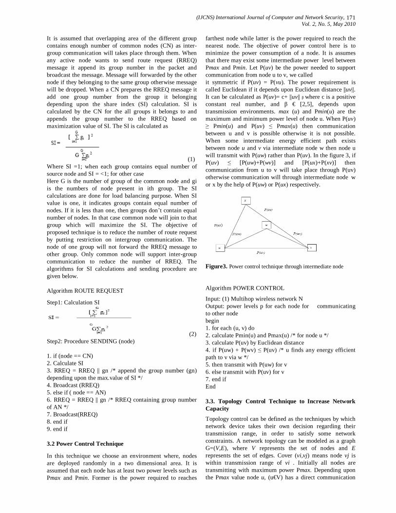
(IJCNS) International Journal of Computer and Network Security, Vol. 2, No. 5, May 2010
171
It is assumed that overlapping area of the different group contains enough number of common nodes (CN) as inter- group communication will takes place through them. When any active node wants to send route request (RREQ) message it append its group number in the packet and broadcast the message. Message will forwarded by the other node if they belonging to the same group otherwise message will be dropped. When a CN prepares the RREQ message it add one group number from the group it belonging depending upon the share index (SI) calculation. SI is calculated by the CN for the all groups it belongs to and appends the group number to the RREQ based on maximization value of SI. The SI is calculated as
(1) Where SI =1; when each group contains equal number of source node and SI = <1; for other case Here G is the number of group of the common node and gi is the numbers of node present in ith group. The SI calculations are done for load balancing purpose. When SI value is one, it indicates groups contain equal number of nodes. If it is less than one, then groups don’t contain equal number of nodes. In that case common node will join to that group which will maximize the SI. The objective of proposed technique is to reduce the number of route request by putting restriction on intergroup communication. The node of one group will not forward the RREQ message to other group. Only common node will support inter-group communication to reduce the number of RREQ. The algorithms for SI calculations and sending procedure are given below. Algorithm ROUTE REQUEST
Step1: Calculation SI
(2) Step2: Procedure SENDING (node) 1. if (node == CN) 2. Calculate SI 3. RREQ = RREQ || gn /* append the group number (gn) depending upon the max.value of SI */ 4. Broadcast (RREQ) 5. else if ( node == AN) 6. RREQ = RREQ || gn /* RREQ containing group number of AN */ 7. Broadcast(RREQ) 8. end if 9. end if 3.2 Power Control Technique In this technique we choose an environment where, nodes are deployed randomly in a two dimensional area. It is assumed that each node has at least two power levels such as Pmax and Pmin. Former is the power required to reaches
farthest node while latter is the power required to reach the nearest node. The objective of power control here is to minimize the power consumption of a node. It is assumes that there may exist some intermediate power level between Pmax and Pmin. Let P(uv) be the power needed to support communication from node u to v, we called it symmetric if P(uv) = P(vu). The power requirement is called Euclidean if it depends upon Euclidean distance ||uv||. It can be calculated as P(uv)= c+ ||uv|| β where c is a positive constant real number, and β € [2,5], depends upon transmission environments. max (u) and Pmin(u) are the maximum and minimum power level of node u. When P(uv) ≥ Pmin(u) and P(uv) ≤ Pmax(u) then communication between u and v is possible otherwise it is not possible. When some intermediate energy efficient path exists between node u and v via intermediate node w then node u will transmit with P(uw) rather than P(uv). In the figure 3, if P(uv) ≤ [P(uw)+P(wv)] and [P(ux)+P(xv)] then communication from u to v will take place through P(uv) otherwise communication will through intermediate node w or x by the help of P(uw) or P(ux) respectively.
Figure3. Power control technique through intermediate node Algorithm POWER CONTROL
Input: (1) Multihop wireless network N Output: power levels p for each node for communicating to other node begin 1. for each (u, v) do 2. calculate Pmin(u) and Pmax(u) /* for node u */ 3. calculate P(uv) by Euclidean distance 4. if P(uw) + P(wv) ≤ P(uv) /* u finds any energy efficient path to v via w */ 5. then transmit with P(uw) for v 6. else transmit with P(uv) for v 7. end if End 3.3. Topology Control Technique to Increase Network Capacity
Topology control can be defined as the techniques by which network device takes their own decision regarding their transmission range, in order to satisfy some network constraints. A network topology can be modeled as a graph G=(V,E), where V represents the set of nodes and E represents the set of edges. Cover (vi,vj) means node vj is within transmission range of vi . Initially all nodes are transmitting with maximum power Pmax. Depending upon the Pmax value node u, (u€V) has a direct communication

(IJCNS) International Journal of Computer and Network Security, Vol. 2, No. 5, May 2010
172
set known as DCS (u). P(uv) denotes the minimum power required for node u to communicate directly to node v. By applying topology control we have to get sub graph G'= (V, E') of G, in G' the node has shorter and fewer numbers of edges as compare to G. The objective of topology control here is to remove the energy-inefficient link from the network. Initially all the node in the network will calculate their DCS depending upon their maximum transmission power. Each node will maintain a node information table containing information like neighbor_id (NI), direct_communication_cost(DCC),and energy_efficient_cost (EEC). Each node has a unique NI. DCC represents the minimum transmission power required for a specific neighbor node. DCC of node u to neighbor node v is represented as DCC(uv) which is same as P(uv) as described earlier. EEC is initially same as DCC but when any energy efficient path is obtained through alternate path ECC is updated. Each node periodically updates their node information table and broadcast the information to other node. After a specific time each node will calculate their DCS by removing energy-inefficient link (if any). \ Algorithm LINK REMOVAL Input: (1) Multihop wireless network G=(V,E), (2) Maximum transmission power Output: G'= (V, E') , G' has shorter and fewer numbers of edges as compare to G Begin 1. Each node broadcast a ―hello" message with its node information table. 2. If a node u receives the ―hello" message from its neighbor 3. If u has a power efficient path to node v via k /* k is a node in alternate path */ 4. update (v, P(uv), P(uk) + P(kv) ) into u’s node information table. /* energy_efficient_cost =( P(uk) + P(kv )) ≤ P(uv) */ 5. Else Insert (v, P(uv), P(uv ) into u’s node information table./*asenergy_efficient_cost = direct_communication_cost*/ 6. End if. 7. End if. End 4. Simulation Results In order to evaluate our power control approach simulation area of 500mt×500mt were taken. We consider scenario1 with six numbers of nodes and scenario2 with five numbers of nodes. Nodes are randomly deployed and are in transmission ranges of each other. In the first scenario different nodes are placed in different position as shown in the figure 3. In scenario 1, it is assumed that one hop communication between sources to destination exists. It means that source to destination path exist through only one intermediate node other than direct path. In scenario 2 multi hop communication has been taken into consideration. In both scenarios node is taken as the source and node 2 is
the destination, it is founds that five alternate paths exists in scenarios 1 and sixteen in scenarios 2. The energy consumption of each path is measured and it is found that path through node3 is least. In the scenario 2 five nodes are placed as shown in the right hand side figure 4. From the simulation results we measure the energy consumption of all paths. In both scenarios energy efficient path is the through node3 although the position of the node3 is different. It is also observed that in single hop count when the angle of the intermediate node is more than ninety degree the alternate path through intermediate node is always energy efficient. In the first scenario the direct path consumes energy proportional to 3.200000e+001. and the path through node3 consumes energy proportional to 1.600000e+001.In the second diagram direct path consume the energy same as first scenario but the energy efficient path through node3 consumes less which is measured and found proportional to 18. From the both scenario we shows that energy consumption in intermediate path is better in comparison to direct path in most of the time.
Figure 4. Energy efficient path through intermediate node 5. Energy Analysis of Routing Protocols There have been several network routing protocols proposed for wireless networks that can be examined in the context of wireless sensor networks. We examine two such protocols, namely direct communication with the base station and minimum-energy multi-hop routing using our sensor network and radio models.
(3)
(4) In addition, we discuss a conventional clustering approach to routing and the drawbacks of using such an approach when the nodes are all energy-constrained using a direct communication protocol, each sensor sends its data directly to the base station. If the base station is far away from the nodes, direct communication will require a large amount of transmit power from each node (since d in Equation 1 is large). This will quickly drain the battery of the nodes and reduce the system lifetime. However, the only receptions in this protocol occur at the base station, so if either the base station is close to the nodes, or the energy required to receive data is large, this may be an acceptable (and possibly optimal) method of communication. The second conventional approach we consider is a “minimum-energy” routing protocol. There are several power-aware routing
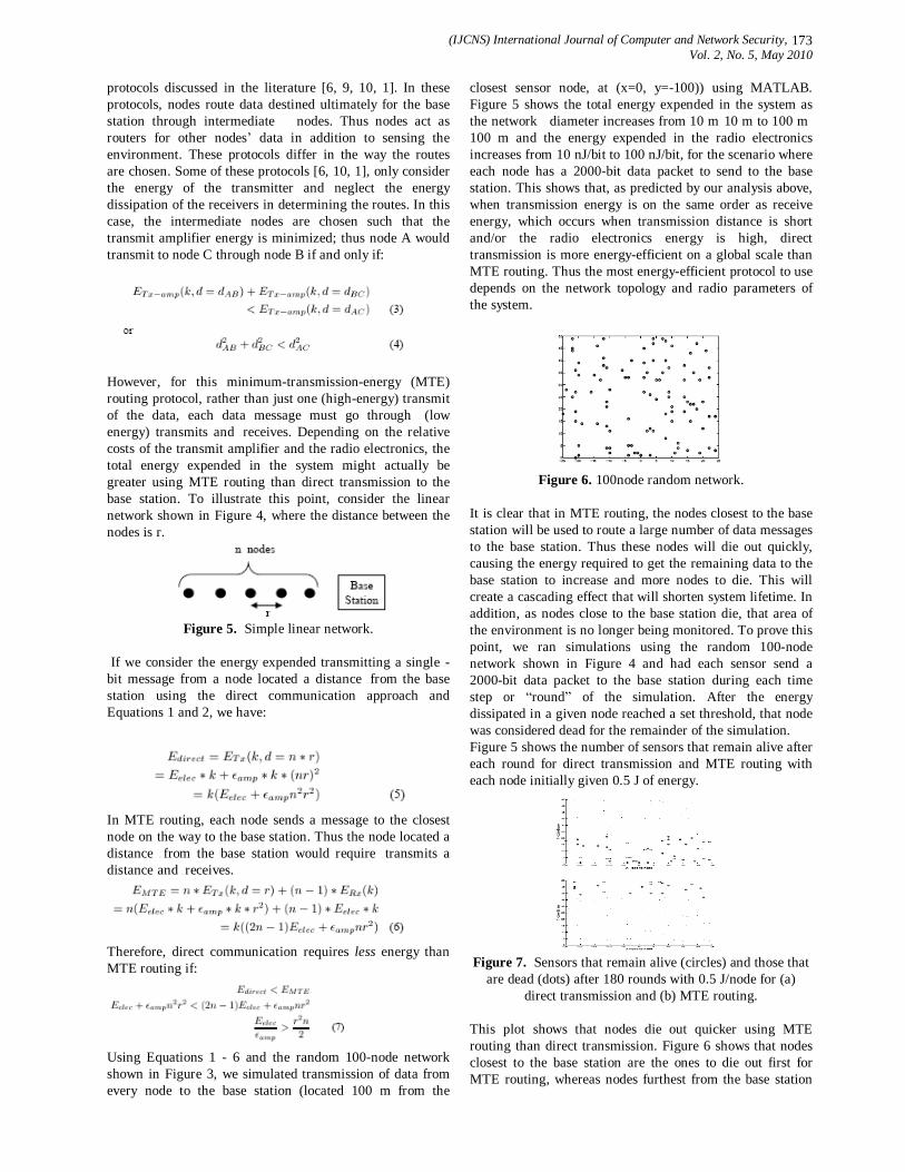
(IJCNS) International Journal of Computer and Network Security, Vol. 2, No. 5, May 2010
173
protocols discussed in the literature [6, 9, 10, 1]. In these protocols, nodes route data destined ultimately for the base station through intermediate nodes. Thus nodes act as routers for other nodes’ data in addition to sensing the environment. These protocols differ in the way the routes are chosen. Some of these protocols [6, 10, 1], only consider the energy of the transmitter and neglect the energy dissipation of the receivers in determining the routes. In this case, the intermediate nodes are chosen such that the transmit amplifier energy is minimized; thus node A would transmit to node C through node B if and only if:
However, for this minimum-transmission-energy (MTE) routing protocol, rather than just one (high-energy) transmit of the data, each data message must go through n (low energy) transmits and n receives. Depending on the relative costs of the transmit amplifier and the radio electronics, the total energy expended in the system might actually be greater using MTE routing than direct transmission to the base station. To illustrate this point, consider the linear network shown in Figure 4, where the distance between the nodes is r.
Figure 5. Simple linear network.
If we consider the energy expended transmitting a single k-bit message from a node located a distance nr from the base station using the direct communication approach and Equations 1 and 2, we have:
In MTE routing, each node sends a message to the closest node on the way to the base station. Thus the node located a distance nr from the base station would require n transmits a distance r and n 1 receives.
Therefore, direct communication requires less energy than MTE routing if:
Using Equations 1 - 6 and the random 100-node network shown in Figure 3, we simulated transmission of data from every node to the base station (located 100 m from the
closest sensor node, at (x=0, y=-100)) using MATLAB. Figure 5 shows the total energy expended in the system as the network diameter increases from 10 m _ 10 m to 100 m _
100 m and the energy expended in the radio electronics increases from 10 nJ/bit to 100 nJ/bit, for the scenario where each node has a 2000-bit data packet to send to the base station. This shows that, as predicted by our analysis above, when transmission energy is on the same order as receive energy, which occurs when transmission distance is short and/or the radio electronics energy is high, direct transmission is more energy-efficient on a global scale than MTE routing. Thus the most energy-efficient protocol to use depends on the network topology and radio parameters of the system.
Figure 6. 100node random network.
It is clear that in MTE routing, the nodes closest to the base station will be used to route a large number of data messages to the base station. Thus these nodes will die out quickly, causing the energy required to get the remaining data to the base station to increase and more nodes to die. This will create a cascading effect that will shorten system lifetime. In addition, as nodes close to the base station die, that area of the environment is no longer being monitored. To prove this point, we ran simulations using the random 100-node network shown in Figure 4 and had each sensor send a 2000-bit data packet to the base station during each time step or “round” of the simulation. After the energy dissipated in a given node reached a set threshold, that node was considered dead for the remainder of the simulation. Figure 5 shows the number of sensors that remain alive after each round for direct transmission and MTE routing with each node initially given 0.5 J of energy.
Figure 7. Sensors that remain alive (circles) and those that
are dead (dots) after 180 rounds with 0.5 J/node for (a) direct transmission and (b) MTE routing.
This plot shows that nodes die out quicker using MTE routing than direct transmission. Figure 6 shows that nodes closest to the base station are the ones to die out first for MTE routing, whereas nodes furthest from the base station
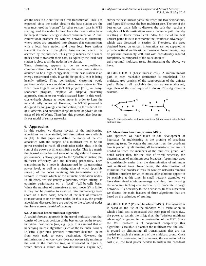
(IJCNS) International Journal of Computer and Network Security, Vol. 2, No. 5, May 2010
174
are the ones to die out first for direct transmission. This is as expected, since the nodes close to the base station are the ones most used as “routers” for other sensors’ data in MTE routing, and the nodes furthest from the base station have the largest transmit energy in direct communication. A final conventional protocol for wireless networks is clustering, where nodes are organized into clusters that communicate with a local base station, and these local base stations transmit the data to the global base station, where it is accessed by the end-user. This greatly reduces the distance nodes need to transmit their data, as typically the local base station is close to all the nodes in the cluster. Thus, clustering appears to be an energy-efficient communication protocol. However, the local base station is assumed to be a high-energy node; if the base station is an energy-constrained node, it would die quickly, as it is being heavily utilized. Thus, conventional clustering would perform poorly for our model of micro sensor networks. The Near Term Digital Radio (NTDR) project [7, 9], an army-sponsored program, employs an adaptive clustering approach, similar to our work discussed here. In this work, cluster-heads change as nodes move in order to keep the network fully connected. However, the NTDR protocol is designed for long-range communication, on the order of 10s of kilometers, and consumes large amounts of power, on the order of 10s of Watts. Therefore, this protocol also does not fit our model of sensor networks. 6. Approaches In this section we discuss several of the multicasting algorithms we have studied; full descriptions are available in [10]. In this paper we define the notion of the cost associated with the support of a multicast tree to be the power required to reach all destination nodes; thus, it is the sum of the powers at all transmitting nodes. This is a metric that is used as the basis of some of our algorithms. However, performance is always judged by the “yardstick” metric, the multicast efficiency, and the blocking probability. Each transmission by a node is characterized by its transmitter power level, as well as a designation of which (possibly several) of the nodes receiving this transmission are to forward it toward which of the ultimate destination nodes. In all cases, we use greedy algorithms, which attempt to optimize performance on a “local” (call-by-call) basis. When the number of transceivers at each node (T) is finite, it may not be possible to establish minimum-energy trees (even on a local basis) because of the lack of resources (transceivers) at one or more nodes. In this case, the greedy algorithms discussed here are applied to the subset of nodes that have non-zero residual capacity. 6.1. A unicast-based multicast algorithm A straightforward approach is the use of multicast trees that consist of the superposition of the best unicast paths to each individual destination (see, e.g., [2]). It is assumed that an underlying unicast algorithm (such as the Bellman–Ford or Dijkstra algorithm) provides “minimum-distance” paths from each node to every destination. However, the minimization of unicast costs does not necessarily minimize the cost of the multicast tree, as illustrated in figure 5, which shows a source and two destinations. Figure 5(a)
shows the best unicast paths that reach the two destinations, and figure 5(b) shows the best multicast tree. The use of the best unicast paths fails to discover the path that reaches a neighbor of both destinations over a common path, thereby resulting in lower overall cost. Also, the use of the best unicast paths fails to incorporate the “multicast advantage,” which was discussed in section 3. Therefore, the trees obtained based on unicast information are not expected to provide optimal multicast performance. Nevertheless, they do perform reasonably well, and with considerably reduced complexity as compared to the calculation of truly optimal multicast trees. Summarizing the above, we have: ALGORITHM 1 (Least unicast cost). A minimum-cost path to each reachable destination is established. The multicast tree consists of the superposition of the unicast paths. Paths to all reachable destinations are established, regardless of the cost required to do so. This algorithm is scalable.
Figure 9. Unicast-based vs multicast-based trees: (a) best unicast paths,(b) best multicast tree. 6.2. Algorithms based on pruning MSTs One approach we have taken in the development of heuristics for multicasting is the pruning of broadcast spanning trees. To obtain the multicast tree, the broadcast tree is pruned by eliminating all transmissions that are not needed to reach the members of the multicast group. We noted earlier that, for the case of wired networks, the determination of minimum-cost broadcast (spanning) trees is considerably easier than the determination of minimum cost multicast trees. Nevertheless, the determination of minimum-cost broadcast trees for wireless networks remains a difficult problem for which no scalable solutions appear to be available at this time. In small network examples we have determined minimum-energy spanning trees by using the recursive technique of section .3; in moderate to large networks it is necessary to use heuristics. In this subsection we discuss the main features of three algorithms that are based on the technique of pruning. ALGORITHM 2 (Pruned link-based MST). This algorithm is based on the use of the standard MST formulation in which a link cost is associated with each pair of nodes (i.e., the power to sustain the link); thus, the “wireless multicast advantage” is ignored in the construction of the MST. Since the MST problem is of polynomial complexity, this algorithm is scalable. To obtain the multicast tree, the MST is pruned by eliminating all transmissions that are not needed to reach the members of the multicast group. Once the MST is constructed in this manner, the evaluation of its cost (i.e., the total power needed to sustain the broadcast
(IJCNS) International Journal of Computer and Network Security, Vol. 2, No. 5, May 2010
175
tree) does take into consideration the wireless multicast advantage. ALGORITHM 3 (Pruned node-based MST). This algorithm requires the determination of the minimum-energy spanning tree that is rooted at the Source node. Unlike algorithm 2, the wireless multicast advantage is taken into consideration in the determination of the power needed to sustain the tree. The recursive algorithm of section .3 can be used to determine the MST. Thus, this method is not scalable. Once the MST has been determined in this manner, it is pruned as in algorithm 2. ALGORITHM 4 (Pruned node-based spanning tree). A heuristic is used to determine a suboptimal spanning tree.10 Once the spanning tree has been determined in this manner, it is pruned as in algorithm 2. Construction of the spanning tree begins at the Source node. Its transmission power is chosen to maximize the following “n/p” metric:
At the next stage, each of the nodes that has been “covered” (i.e., the Source node plus all nodes within its communication range based on the calculation in the first stage) evaluates the n/p metric for all possible sets of neighbors (however, in computing this metric, only “new” nodes, i.e., nodes not previously covered, are included in the number of destinations). Note that it is possible to increase the transmission power that was assigned to a node in an earlier stage. This procedure is repeated until all nodes are covered. 6.3. Additional algorithms with high complexity The following algorithms require an exhaustive search, and are thus not scalable. Nevertheless, they provide a useful benchmark that permits us to evaluate the performance of the other algorithms for small network examples. ALGORITHM 5 (Least multicast cost). As in algorithm 1, paths to all reachable destinations are established, regardless of the cost required to do so. An exhaustive search of all multicast trees that reach all reachable destinations is performed. The tree with the lowest cost is chosen. ALGORITHM 6 (Maximum local yardstick). The local yardstick function yi is computed for each arriving multicast request i. Multicast trees are formed to all subsets of intended destinations. The tree that results in the maximum value of yi is chosen. This tree does not necessarily include all reachable destinations. 6.4 Energy efficient greedy scheme The concept of neighbor classification based on node energy level and their distances has been used in Energy Efficient Greedy Scheme (EEGS) has been used to cater of the weak node problem. Some neighbors may be more favorable to
choose than the others, not only based on distance, but also based on energy characteristics. It suggests that a neighbor selection scheme should avoid the weak nodes. If the geographic forwarding scheme purely based on greedy forwarding attempts to minimize the number of hops by maximizing the geographic distance covered at each hop, it is likely to incur significant energy expenditure due to retransmission on the weak nodes. On the other hand, if the forwarding mechanism attempts to maximize per hop reliability by forwarding only to close neighbors with good nodes, it may cover only small geographic distance at each hop. It would also result in greater energy expenditure due to the need for more transmission hops for each packet to reach the destination. So in both cases energy is not being conserved to increase the lifetime of the network. Therefore, the strategy used in the proposed Energy Efficient Greedy Scheme (EEGS) first calculates the average distance of all the neighbors of transmitting node and checks their energy levels. Finally, it selects the neighbor which is alive (i.e. having energy level above than the set threshold) and having the maximum energy plus whose distance is equal to or less than the calculated average distance among its entire neighbors. Hence, the proposed scheme uses Energy Efficient routing to select the neighbor that has sufficient energy level and is closest to the destination for forwarding the query. 7. Conclusion In this paper we have argued that optimal techniques and approaches for enhancing the communication and data exchange between wireless networks. The schemes discussed in the paper reduce the overall energy, while our spreading approaches aim at distributing the traffic in a more balanced way. We note that our basic ideas and techniques should be able to enhance other routing protocols as well. Also In this paper, we reviewed some of the recent work done in mobile ad hoc network considering energy as the key issue. It is found that most of the study discusses the energy issue at data link and network layer. We suggest three energy efficient techniques for MANET point of view. Route request minimization technique can be done by implementing logical grouping; power control techniques reduce the transmission power of a node while topology control approach increases the network longevity by satisfying network constraints. The simulation results presented in section 4.0, suggests that multi-hop is ideal for energy point of view but the limitation is the increase chance of link failure. References [1] C.E.Perkins, "Ad Hoc Networking", Addison Wesley,
2001. [2] IEEE 802.11 Working Group, "Wireless LAN Medium
Access Control (MAC) and Physical Layer (PHY) Specification",1999.
[3] D.Zhou and.T.H.Lai, " A scalable and adaptive clock synchronization protocol for IEEE 802.11-based multihop ad hoc networks," IEEE International
(IJCNS) International Journal of Computer and Network Security, Vol. 2, No. 5, May 2010
176
Conference on Mobile Ad hoc and Sensor Systems Conference, 2005 , Nov 2005.
[4] S.Singh and C.S.Raghavendra, "PAMAS power aware multi-access protocol with signaling for ad hoc networks," ACM Computer Communication Review, vol. 28(3), pp.5-26, July 1998.
[5] L.M. Freeny, ―Energy efficient communication in ad hoc networks," Mobile Ad Hoc Networking, Wiley-IEEE press, pp.301-328, 200.
[6] E.S.Jung and N. H. Vaidya, "An energy efficient MAC protocol for wireless LANs," IEEE INFOCOM, June 2002.
[7] [E.S.Jung and N.H.Vaidya, "A Power Control MAC Protocol for Ad Hoc Networks," ACM Intl. Conf. Mobile Computing and Networking (MOBICOM), September 2002.
[8] B.Chen,K.Jamieson,H.Balakrishnan and R.Morris, "Span:An energy efficient coordination algorithm for topology maintenance in ad hoc wireless networks," ACM Wireless Networks Journal, vol. 8(5), pp. 81-9, September 2002.
[9] P.K.Sahoo,J.P.Sheu and K.Y.Hsieh, ―Power control based topology construction for the distributed wireless sensor networks," Science Direct,Computer Communications, vol. 30, pp. 277-2785, June 2007.
[10] R. Ramanathan, R. Rosales-Hain, Topology control of multihop wireless networks using transmit power adjustment, in:Proceedings of the 19th INFOCOM, Tel Aviv, Israel, March 2000, pp. 0–13.
[11] Barrenechea, G.; Beferull-Lozano, B. & Vetterli, M.(200). “Lattice Sensor Networks:Capacity Limits, Optimal Routing and Robustness to Failures,” Proceedings of thethird international symposium on Information processing in sensor networks, pp. 186–195,Berkeley, California, April 200.
Authors Profile
Dr. Neeraj Tyagi has completed B.E. degree in Computer Science & Engineering from Motilal Nehru National Institute of Technology, Allahabad (Uttar Pradesh) in 1987, his M.E. degree in Computer Science & Engineering from MNNIT, Allahabad (Uttar Pradesh) in 1997 and PhD degree in Computer Science & Engineering from
MNNIT, Allahabad (Uttar Pradesh) in 2008.His teaching and research interests including Computer Networks, Mobile Ad-Hoc Networks, wireless Networks and Operating Systems. He joined the department of Computer Science & Engineering in 1989 at MNNIT, Allahabad and he has Also worked in Warman International- Australia, G.E (Capital) - U.S.A, Electronic Data Systems- U.S.A during 1999-2001. Presently he is working as Associate Professor in the department of Computer Science & Engineering, MNNIT, Allahabad(Uttar Pradesh), India.
Awadhesh Kumar graduated from Govind Ballabh Pant Engineering college, Pauri (Garhwal) in Computer Science & Engineering in 1999. He obtained his Master degree (M.Tech.) in Computer Science from Uttar Pradesh Technical University, Lucknow in 2006. He joined the department
of Computer Science & Engineering at Kamla Nehru Institute of Technology, Sultanpur (Uttar Pradesh) as Lecturer in 2000 and became Assistant Professor in 2007. His teaching and research interests include Computer Networks, Wireless Networks and Mobile Ad-Hoc Networks. He is pursuing PhD program in the department of Computer Science & Engineering, MNNIT, Allahabad (Uttar Pradesh) in the area of Mobile Ad-hoc Networks.
Ajeet Kumar Post graduated from Madan Mohan Malaviya Engineering college, Gorakhpur (U.P.) in Master of Computer Application 2003. I pursuing our Master degree (M.Tech.) in Software Engineering from SRMS CET Bareilly affiliated to Uttar Pradesh Technical University, Lucknow. I have joined the department of Master of Computer Application in SRMS CET Bareilly (Uttar Pradesh) as Lecturer in 2003. His teaching and
research interests include Object Oriented System, Software Engineering, Mobile Computing, Wireless Networks and Mobile Ad-Hoc Networks.
Rati Agarwal received her B.Tech degree from Uttar Pradesh Technical University Lucknow. She is pursuing M.Tech from Karnataka University. Presently, she is working as a Lecturer (CS/IT Deptt) in SRMSWCET, Bareilly. She has written a book on “Soft Computing”. She has attended a faculty development program based on “Research methodologies” and has also undergone a training in Infosys Campus
Connect Program held at S.R.M.S.C.E.T. Bareilly.

(IJCNS) International Journal of Computer and Network Security, Vol. 2, No. 5, May 2010
177
Centralized Framework for Real Time Traffic in Vehicular Ad hoc Networks
Nazish Khan1, Dr. Anjali Mahajan2
1IV Semester M.E. Wireless Communication and Computing,
Computer Science and Engineering Department, G. H. Raisoni College of Engineering, Nagpur, India
2Professor, Department of Information Technology, G. H. Raisoni College of Engineering, Nagpur, India
[email protected] Abstract: Vehicular networks are formed by vehicles communicating in an ad hoc manner or through cellular and IEEE 802.11 base stations. Routing in vehicular networks is challenging due to highly dynamic network topologies. Previous research done has proposed the idea of Road-Based using Vehicular Traffic information (RBVT) routing. In RBVT, routes are sequences of road intersections, and geographical forwarding is used for sending packets between the intersections. This paper proposes centralized framework for real time traffic in Vehicular Ad hoc NETworks (VANETs). Already available protocols are completely distributed protocol that unicasts connectivity packets in the network to find the roadbased topology graph. This graph represents a real-time view of the roads with enough vehicular traffic to ensure connectivity between intersections and is disseminated to all nodes. Proposed framework uses a similar concept, but the road connectivity information is gathered and sent separately to a server via cellular links. The server centrally computes the connectivity graph and disseminates it to the nodes in the network. The proposed framework is compared against existing routing protocols. Simulation results for city scenarios show that the proposed framework performs better than the existing protocols, with reduction in end-to-end delay and increase in delivery ratio.
Keywords: VANETs, Dissemination, Centralized Information Packet, Wi-Fi Link, Cellular Communication.
1. Introduction In recent years there has been a growing interest in field of vehicular networks, primarily due to the advancement in technology and need for safety and entertainment applications. The current generation of vehicles have embedded computers, GPS receivers, and number of sensors, whereas the next generation of these vehicles will potentially have short-range wireless network interfaces and wireless access to the Internet. A vehicular network in general is a network of vehicles that can communicate with each other; the network could be formed by use of infrastructure such as cellular or road side fixed equipment or on-the-fly in an ad hoc manner. The vehicular network that is formed in ad hoc manner without need of infrastructure is called a Vehicular Ad-hoc NETwork (VANET). One of the core issues of vehicular networks is designing efficient and scalable routing protocols. Such protocols are
needed for most of the applications to come to reality. The development of new routing protocols is important because not only will they enable the addition of new dimensions to the vehicle through various applications in areas such as vehicular safety, but they will also transform it from being a mere transportation means to a smart vehicle. The requirements of routing protocol in VANET are significantly different than what they are in wired network or Mobile Ad hoc NETwork (MANET). Some of the major differences in VANET are (i) Mobility: due to which the topology is highly dynamic, (ii) Road layout: a node moves on the road, which constraint the packet to follow the road path, and (iii) Obstacles: due to which the communication on close-by parallel streets is restricted. In past, the research has been focused on finding variants to MANET protocols and changing some of their parameters (to overcome issue of highly dynamic topologies) or developing reactive/geographical VANET protocols. Some of these protocols [11][12] do use the right approach of using road intersections as part of their routes but fail to use the real time traffic information or propose an expensive solution of deploying infrastructure such as deploying sensors to get the real-time traffic information.
2. Related Work The research group in the UbiNetS lab at NJIT proposed Road-Based using Vehicular Traffic (RBVT) routing. As the name suggests, RBVT leverages real-time vehicular traffic information to create road-based routes. The created routes are successions of the road intersections that have, with high probability, network connectivity between them. A packet between consecutive intersections is forwarded using Geographical routing; this approach decouples routes from individual node movements. There are two main advantages in RBVT: (a) adaptability to topological changes by incorporating real-time vehicular traffic information and (b) stability in route by use of road-based routes and geographical forwarding. Route Construction: Routing is a process of moving packets through the network. It consists of two separate, but related, tasks: (a) Defining paths for the transmission of packets through the network and (b) Forwarding packets based upon the defined paths. The tasks are achieved with the help of routing table. RBVT being proactive protocols

(IJCNS) International Journal of Computer and Network Security, Vol. 2, No. 5, May 2010
178
the routes tables are updated for every known change of topology. Usually the protocols [8, 9, 10] that have been derived from MANET use node centric approach, these protocols do not work well due to the dynamic nature of the network. The other protocols [11, 13, 14, 15] use the road-based approach, these protocols use the right approach but most of them [11, 15] do not factor in the current road traffic and rather try to use the shortest distance to reach from source to destination, which currently may not have any traffic. The protocols fail to consider traffic flow; some of the protocols [14, 12, 16, 17] try to work around this problem by using historic data. Due to the events such as road constructions or traffic redirections which are not rare, the historical data does not remain an accurate indicator of the current road traffic flow. The RBVT protocols use road intersection as their building block. When a source wants to transfer data to the destination, instead of tying particular nodes to the route towards the destination it uses the road intersections. As long as the road segments remain connected it does not matter if the connectivity between the individual nodes on a road segment exists. The fault in binding a particular node to a route is due to the node movement, it may not remain in the sight of the route. Forwarding: A node periodically broadcasts hello messages; the receiving node updates its neighbor table using the information provided in hello message. If a hello message is not received from a particular neighbor within a time interval the entry is purged; non-receipt of hello messages is a strong indication that the other node is travelled out of communication range. When the source node wants to transmit data to destination node, it queries the routing table for the available routes to the destination; if there are multiple routes from the source to destination, the route with minimum number of intersections is used. This desired route is stored in the packet for reference of the intermediate node. The protocol uses loose source routing to forward data packets in order to improve the routing performance. The intermediate nodes are free to change the path in the packet if they have latest connectivity information. The node that stores or updates the route information in the packet also writes the timestamp of the connectivity graph that was used for determining this route. The intermediate node compares its connectivity graph timestamp to decide if a better routing decision can be made. Due to the high volatility there could be route breaks, in such cases the intermediate node tries forwarding the data packet using geographical forwarding method until it reaches a node that has fresher information and there exists a route from that node to the destination; this newly found route is updated in the packet and forwarded further towards the next intersection. In between intersections the packet is forwarded using geographical forwarding; this is advantageous as the node always selects the farthest possible neighbor node to forward the packet. In this class of routing there are particularly two advantages: (a) it is adaptive to network topology changes by using real-time vehicular traffic information and (b) the stability of route through road-based routes and use of geographical forwarding.
2.1 RBVT-P RBVT-P is a proactive routing protocol for VANET; it periodically discovers and disseminates the real-time road connectivity graph. The source node uses the connected shortest available path to the destination. The path consists of intersections that are found connected in the real-time view. RBVT-P uses a location service, to find the destination position. Due to the dynamic nature of the network, RBVT-P does not bind the forwarding of packets to a particular node like AODV (which are node centric). Topology Discovery: The topology is discovered by use of Connectivity Packet (CP). The CP is a packet that traverses the connected road segments and stores the visited intersections in it. This information is later used to create the connectivity graph which is then disseminated in the network to other nodes. The CPs are generated periodically by a number of randomly selected nodes in the network. The CP packet traverses the road intersection by use of algorithm similar to DFS graph traversal, as the packet moves from one intersection to other intersection the road segment is marked as connected otherwise as un-connected. The CPs are periodically generated by a CP generator node, they are unicasted to discover the network topology. Topology Dissemination and Route Computation: The node that finally receives the CP on the generator segment extracts the information in the CP to generate a Connectivity Graph Update (CGU) packet and disseminates the CGU to other nodes in the connected network. Upon receiving the latest CGU, each node updates its routing table and re-computes the shortest paths to all other connected intersections. One of the fields of each entry in CGU is timestamp, with the use of this field the node determines whether the information it already has or the information the CGU contains is the latest one. The timestamp of each entry is retained in the routing table to identify and remove the stale entries at later point of time. When the source has to transmit information to the destination it determines and uses the shortest path through the connected intersections. The path is made of sequence of intersections and is stored in the header of the data packet. The packet is forwarded geographically between the consecutive intersections, defined in the path. The protocol uses loose source routing so the intermediate node is free to update the path if it has more recent information about the topology. Route Maintenance: The RBVT-P generates CP frequently (which in turn generates CGU) that keeps the nodes updated with the topological changes. The CPs are generated from different section of the network so that the information of particular section is gathered by the nodes in that section. The node in an isolated section cannot know the connectivity information about other section till the disconnection between these isolated networks is bridged. The frequency of generating CP would depend on the network size and density of nodes in the section of the network. Higher the density, lower number of packets are required as the probability of finding the replacement node increases. In a CP generation interval, multiple CP are generated to avoid the problem of loosing connectivity information in a CP round when CP packet is lost. The CP

(IJCNS) International Journal of Computer and Network Security, Vol. 2, No. 5, May 2010
179
passing protocol is not a reliable protocol but a best effort delivery so there are chances of them getting lost.
3. Proposed Work Importance of this proposed solution come from the use of real-time traffic information and the way route between the source and destination is created. Unlike the MANET protocols, the proposed framework use road intersections as a part of route. Road intersections are stationary; having them in route is more advantageous than having a moving vehicle. The difference with respect to other VANET protocol is that the proposed solution use real-time traffic information rather than the historic data. The use of road intersection as the guiding point helps when a moving vehicle goes out of range from the guided point. This vehicle (that moved out of range) can be replaced with other vehicle near the road intersection to forward the packet towards the destination. The need for such mechanism arises due to the highly dynamic changes in the topology. The proposed framework being proactive is expected to be better in terms of end to end delay i.e. lowering the delay of end to end communication.
3.1 Design Centralized framework for real time traffic in Vehicular Ad hoc NETworks uses the concept of proactive protocol. It uses a concept called as Centralized Information Packet (CIP) that is similar to CP used in RBVT-P. The car node on the road considers itself the most forward if it does not receive any packet for a timeout interval; similarly it considers itself most backward if it does not find any node to which it can send the CIP. The nodes backward/forward direction is irrespective of the driving direction; each road in the map is assigned a direction that is stored along with digital map in the node. The communication between the node and the server takes place using the Cellular technology whereas the communication between the nodes is through Wi-Fi wireless technology.
Topology Discovery: The most forward node on the road sends the CIP to the node behind it. The intermediate node continues forwarding this packet to the node behind it, eventually reaching the most backward node (no other node behind it on that road which this backward node can communicate). This most backward positioned node on the road sends the gathered connectivity information through its GPRS interface to the server. The connectivity information entry is of the form <FirstIntersectionID, LastIntersectionID, ExpirationTime>; where FirstIntersectionID indicates the intersection id from where the connectivity begins, LastIntersectionID indicates the end intersection till the connectivity on the road segments exists and the ExpirationTime indicates the time till the road segments are valid. The expiration time is calculated by addition of Maximum connectivity valid period (protocol configurable value) and current time. The connectivity information is gathered for the segments through which a CIP traveled. The CIP may also implicitly indicate the nonconnectivity of two segments the one before the
FirstIntersectionID and the one after LastIntersectionID to the block of connected segments. The server receives one CIP from each set of connected nodes; there can be multiple CIPs for the same road depending on the connectivity pattern on the road. For e.g. in Figure 1 on road segment S1 of road R3, the five nodes create an isolated network from the nodes on segment S2 on the same road, in these cases there are two different CIPs that are sent to the server from these two sections on the same road. In the figure R1, R2 and R3 indicate roads and S1, S2 and S3 designate the segments on the roads. The pair <Road><Segment> uniquely identifies the segments. The car nodes on the roads are named N1, N2, N3 and N11.
Figure 1. Most backward cars on the each road send CIP to server. After computing the real-time graph it is sent to the
node which sent this CIP.
The car N1 being the most forward node on road R1 starts a CIP, every node that has the responsibility to send this packet tries to send it the most farthest possible node so that the discovery of information is faster and this also makes the protocol more efficient. In the example N1 skips node N2 and sends the packet directly to N3 as N3 is in the wireless range of N1. The packet is similarly forwarded to the most backward node (in this case N11), which then sends the packet to the server for re-computing the real-time graph. I1 to I8 indicate the intersections or end points of the roads. Topology Dissemination and Route Computation: On receipt of each CIP the server updates the connectivity graph. In comparison with RBVT-P, this same task is done by the node that finally received the CP from the segment where it was initiated (this indicates that an iteration of connected graph is complete). Once the server rebuilds the connectivity graph, it transmits this graph back to the node that sent the CIP that triggered the graph computation. The node then disseminates this information by broadcasting it to the neighbors. This continues till the most forward node receives the information. Similar to RBVT-P each node then runs Dijkstra’s algorithm on the newly received connectivity graph to find the shortest path to all the connected segments in the map. Further on, when a source node wants to transmit data, it stores the connected available shortest path in the packet header. These routes, represented as sequences of intersections, are stored in the data packet headers and
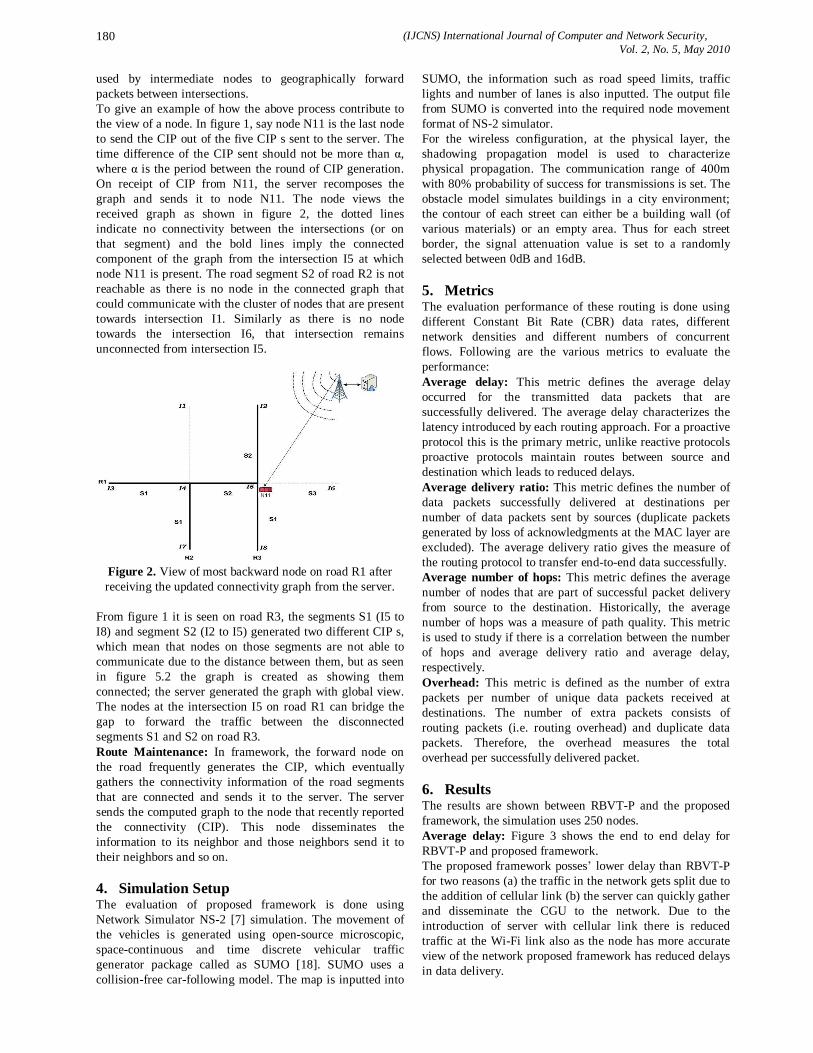
(IJCNS) International Journal of Computer and Network Security, Vol. 2, No. 5, May 2010
180
used by intermediate nodes to geographically forward packets between intersections. To give an example of how the above process contribute to the view of a node. In figure 1, say node N11 is the last node to send the CIP out of the five CIP s sent to the server. The time difference of the CIP sent should not be more than α, where α is the period between the round of CIP generation. On receipt of CIP from N11, the server recomposes the graph and sends it to node N11. The node views the received graph as shown in figure 2, the dotted lines indicate no connectivity between the intersections (or on that segment) and the bold lines imply the connected component of the graph from the intersection I5 at which node N11 is present. The road segment S2 of road R2 is not reachable as there is no node in the connected graph that could communicate with the cluster of nodes that are present towards intersection I1. Similarly as there is no node towards the intersection I6, that intersection remains unconnected from intersection I5.
Figure 2. View of most backward node on road R1 after receiving the updated connectivity graph from the server.
From figure 1 it is seen on road R3, the segments S1 (I5 to I8) and segment S2 (I2 to I5) generated two different CIP s, which mean that nodes on those segments are not able to communicate due to the distance between them, but as seen in figure 5.2 the graph is created as showing them connected; the server generated the graph with global view. The nodes at the intersection I5 on road R1 can bridge the gap to forward the traffic between the disconnected segments S1 and S2 on road R3. Route Maintenance: In framework, the forward node on the road frequently generates the CIP, which eventually gathers the connectivity information of the road segments that are connected and sends it to the server. The server sends the computed graph to the node that recently reported the connectivity (CIP). This node disseminates the information to its neighbor and those neighbors send it to their neighbors and so on. 4. Simulation Setup The evaluation of proposed framework is done using Network Simulator NS-2 [7] simulation. The movement of the vehicles is generated using open-source microscopic, space-continuous and time discrete vehicular traffic generator package called as SUMO [18]. SUMO uses a collision-free car-following model. The map is inputted into
SUMO, the information such as road speed limits, traffic lights and number of lanes is also inputted. The output file from SUMO is converted into the required node movement format of NS-2 simulator. For the wireless configuration, at the physical layer, the shadowing propagation model is used to characterize physical propagation. The communication range of 400m with 80% probability of success for transmissions is set. The obstacle model simulates buildings in a city environment; the contour of each street can either be a building wall (of various materials) or an empty area. Thus for each street border, the signal attenuation value is set to a randomly selected between 0dB and 16dB. 5. Metrics The evaluation performance of these routing is done using different Constant Bit Rate (CBR) data rates, different network densities and different numbers of concurrent flows. Following are the various metrics to evaluate the performance: Average delay: This metric defines the average delay occurred for the transmitted data packets that are successfully delivered. The average delay characterizes the latency introduced by each routing approach. For a proactive protocol this is the primary metric, unlike reactive protocols proactive protocols maintain routes between source and destination which leads to reduced delays. Average delivery ratio: This metric defines the number of data packets successfully delivered at destinations per number of data packets sent by sources (duplicate packets generated by loss of acknowledgments at the MAC layer are excluded). The average delivery ratio gives the measure of the routing protocol to transfer end-to-end data successfully. Average number of hops: This metric defines the average number of nodes that are part of successful packet delivery from source to the destination. Historically, the average number of hops was a measure of path quality. This metric is used to study if there is a correlation between the number of hops and average delivery ratio and average delay, respectively. Overhead: This metric is defined as the number of extra packets per number of unique data packets received at destinations. The number of extra packets consists of routing packets (i.e. routing overhead) and duplicate data packets. Therefore, the overhead measures the total overhead per successfully delivered packet. 6. Results The results are shown between RBVT-P and the proposed framework, the simulation uses 250 nodes. Average delay: Figure 3 shows the end to end delay for RBVT-P and proposed framework. The proposed framework posses’ lower delay than RBVT-P for two reasons (a) the traffic in the network gets split due to the addition of cellular link (b) the server can quickly gather and disseminate the CGU to the network. Due to the introduction of server with cellular link there is reduced traffic at the Wi-Fi link also as the node has more accurate view of the network proposed framework has reduced delays in data delivery.

(IJCNS) International Journal of Computer and Network Security, Vol. 2, No. 5, May 2010
181
Figure 3. Average Delay with density of 250 nodes.
Average delivery ratio: Figure 4 shows the average delivery ratio for RBVT-P and proposed framework. The RBVT-P demonstrates lower delivery ratio performance than the proposed framework as in RBVT-P along with the data packets, the connectivity packets (that gather the real-time connectivity graph of the network) and the CGU packets (that disseminate the collected connectivity graph view) participate in network traffic at Wi-Fi interface. The proposed framework shows 10% gain in delivery ratio this is due to the fact that the control plane traffic of the network is transmitted via cellular link and Wi-Fi link is used for data plane.
Figure 4. Average Delivery Ratio with density of 250 nodes.
7. Conclusion This paper presented the framework for real time traffic environments that take advantage of the road topology to improve the performance of routing in VANET. Simulation results show that the proposed framework outperform existing approaches in terms of average delay, average delivery ratio and low overhead. Because the RBVT protocols forward data along the streets, not across the streets, and take into account the real-time traffic on the roads, they perform well in realistic vehicular environments in which buildings and other road characteristics such as dead end streets, traffic lights are present. As cellular link would more commonly be available, we used a server with cellular communication to show how the performance can increase if the control plane (i.e., routing traffic) is routed across the cellular link whereas data is transmitted over the Wi-Fi link in ad hoc manner.
References [1] Bernd Roessler, Christian Bruns. Replication of Local
Road Networks for Regional Information Dissemination in VANETS. WORKSHOP ON POSITIONING, NAVIGATION AND COMMUNICATION (WPNC’06).
[2] Mitko Shopov, Evtim Peytchev, Generation and dissemination of traffic information in Vehicular Ad-hoc Networks, Computer Science’2005, Technical University of Sofia, Bulgaria.
[3] Emanuel Fonseca, Andreas Festag, Roberto Baldessari, Rui Aguiar, Support of Anonymity in VANETs–Putting Pseudonymity into Practice, IEEE Wireless Communications and Networking Conference (WCNC),Hong Kong, March 2007.
[4] Tarik Taleb, Ehssan Sakhaee, Abbas Jamalipour, Kazuo Hashimoto, Nei Kato, and Yoshiaki Nemoto,
“A Stable Routing Protocol to Support ITS Services in VANET Networks”IEEE TRANSACTIONS ON VEHICULAR TECHNOLOGY, VOL. 56, NO. 6, NOVEMBER 2007
[5] Maria Kihl, Mihail L. Sichitiu, and Harshvardhan P. Joshi “Design and Evaluation of two Geocast Protocols for Vehicular Ad-hoc Networks” JOURNAL OF INTERNET ENGINEERING, VOL. 2, NO. 1, JUNE 2008
[6] Ioannis Broustis and Michalis Faloutsos “Routing in Vehicular Networks: Feasibility, Modeling, and Security” Hindawi Publishing Corporation International Journal of Vehicular Technology Volume 2008, Article ID 267513
[7] The network simulator ns-2 http://www.isi.edu/nsnam/ns2/
[8] Perkins, C. and Royer, E. (1999). Ad hoc On Demand Distance Vector (AODV) Routing. In Proceedings 2nd Workshop on Mobile Computing Systems and Applications. New Orlean s, LA, USA: IEEE, February 1999, pp. 90–100.
[9] Clausen, T. and Jacquet, P. (2003). Optimized Link State Routing Protocol (OLSR). RFC 3626, IETF Network Working Group.
[10] Perkins, C., and Bhagwat, P. (1994). Highly dynamic Destination-Sequenced Distance-Vector routing (DSDV) for mobile computers. SIGCOMM Computer Communication.
[11] Lochert, C., Hartenstein, H., Tian, J., Füßler, H., Hermann, D., and Mauve M. (2003). A routing strategy for vehicular ad hoc networks in city environments. In Proceedings of IEEE Intelligent Vehicles Symposium, pages 156--161.
[12] Jerbi, M., Meraihi, R., Senouci, S., and Ghamri-Doudane Y. (2006). Gytar: improved greedy traffic aware routing protocol for vehicular ad hoc networks in city environments. In Proceedings of the 3rd ACM International Workshop on Vehicular Ad hoc Networks (VANET), Los Angeles, CA, USA, pp. 88–89.
[13] Naumov, V., and Gross, T., (2007). Connectivity-Aware Routing (CAR) in vehicular ad hoc networks.
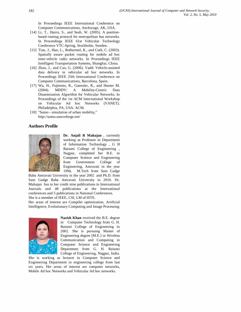
(IJCNS) International Journal of Computer and Network Security, Vol. 2, No. 5, May 2010
182
In Proceedings IEEE International Conference on Computer Communications, Anchorage, AK, USA.
[14] Li, T., Hazra, S., and Seah, W. (2005). A position-based routing protocol for metropolitan bus networks. In Proceedings IEEE 61st Vehicular Technology Conference VTC-Spring, Stockholm, Sweden.
[15] Tian, J., Han, L., Rothermel, K., and Cseh, C. (2003). Spatially aware packet routing for mobile ad hoc inter-vehicle radio networks. In Proceedings IEEE Intelligent Transportation Systems, Shanghai, China.
[16] Zhao, J., and Cao, G. (2006). Vadd: Vehicle-assisted data delivery in vehicular ad hoc networks. In Proceedings IEEE 25th International Conference on Computer Communications, Barcelona, Spain.
[17] Wu, H., Fujimoto, R., Guensler, R., and Hunter M. (2004). MDDV: A Mobility-Centric Data Dissemination Algorithm for Vehicular Networks. In Proceedings of the 1st ACM International Workshop on Vehicular Ad hoc Networks (VANET). Philadelphia, PA, USA: ACM.
[18] “Sumo - simulation of urban mobility,” http://sumo.sourceforge.net/
Authors Profile
Dr. Anjali R Mahajan , currently working as Professor in Department of Information Technology , G H Raisoni College of Engineering , Nagpur, completed her B.E. in Computer Science and Engineering from Government College of Engineering, Amravati in the year 1994, M.Tech from Sant Gadge
Baba Amravati University in the year 2002 and Ph.D. from Sant Gadge Baba Amravati University in 2010. Dr. Mahajan has to her credit nine publications in International Journals and 48 publications at the International conferences and 5 publications in National Conferences. She is a member of IEEE, CSI, LM of ISTE. Her areas of interest are Compiler optimization, Artificial Intelligence, Evolutionary Computing and Image Processing
Nazish Khan received the B.E. degree in Computer Technology from G. H. Raisoni College of Engineering in 2002. She is pursuing Master of Engineering degree [M.E.] in Wireless Communication and Computing in Computer Science and Engineering Department from G. H. Raisoni College of Engineering, Nagpur, India.
She is working as lecturer in Computer Science and Engineering Department in engineering college from last six years. Her areas of interest are computer networks, Mobile Ad hoc Networks and Vehicular Ad hoc networks.
(IJCNS) International Journal of Computer and Network Security, Vol. 2, No. 5, May 2010
183
Energy-efficient Algorithm for a novel clustering approach in w/s networks
S. Sarah 1, P. Kumaran2 and Dr. A. Arul Lawrence Selvakumar 3
1 M. E Final Year, Dr. Paul’s Engineering College, Pondicherry, Anna University, Chennai, Tamilnadu, India
2Assistant Professor, Department of Computer Science and Engineering, Dr. Paul’s Engineering College, Pondicherry, Anna University, Chennai, Tamilnadu, India
3Professor & Head, Department of Computer Science and Information Technology, Kuppam Engineering College, Kuppam, Andhra Pradesh, India
Abstract: Energy efficiency operations are essential in extending Wireless Sensor Networks lifetime. Among the energy saving- based solutions, clustering sensor nodes is an interesting technique for achieving these goals. . In this work, we propose a new energy-efficient approach for clustering nodes in adhoc sensor networks. The main challenge in wireless sensor network deployment pertains to optimizing energy consumption when collecting data from sensor nodes. Compared to other methods (CPLEX-based method, distributed method, simulated annealing-based method), the results show that our approach returns high-quality solutions in terms of cluster cost and execution time. As a result, this approach is suitable for handling network extensibility in a satisfactory manner.
Keywords: wireless sensor networks, clustering, energy- efficient, distributed.
1. Introduction Sensor networks have recently emerged as an important
computing platform. Sensor nodes are typically less mobile and more densely deployed than mobile ad-hoc networks (MANETs). Sensor nodes must be left unattended e.g., in hostile environments, which makes it difficult or impossible to re-charge or replace their batteries (solar energy is not always an option). This necessitates devising novel energy-efficient solutions to some of the conventional wireless networking problems, such as medium access control, routing, self-organization, bandwidth sharing, and security. Exploiting the tradeoffs among energy, accuracy, and latency, and using hierarchical (tiered) architectures are important techniques for prolonging network lifetime This necessity implies the emergence of new kinds of networks, which are typically composed of low-capacity devices. Such devices, called sensors, make it possible to capture and measure specific elements from the physical world (e.g., temperature, pressure, humidity). Moreover, they run on small batteries with low energetic capacities. Consequently, their power consumption must be optimized in order to ensure increased lifetime for those devices.
During data collection, two mechanisms are used to reduce energy consumption: message aggregation and filtering of redundant data. These mechanisms generally use clustering methods in order to coordinate aggregation and filtering. Hierarchical (clustering) techniques can aid in reducing useful energy consumption. Clustering is particularly useful for applications that require scalability to hundreds or thousands of nodes. Scalability in this context implies the need for load balancing and efficient resource utilization. Applications requiring efficient data aggregation (e.g., computing the maximum detected radiation around an object) are natural candidates for clustering. Routing protocols can also employ clustering. Clustering was proposed as a useful tool for efficiently pinpointing object locations. Clustering can be extremely effective in one-to-many, many - to- one, one-to-any, or one-to-all (broadcast) communication. For example, in many-to-one communication, clustering can support data fusion and reduce communication interference. The essential operation in sensor node clustering is to select a set of cluster heads among the nodes in the network, and cluster the rest of the nodes with these heads. Cluster heads are responsible for coordination among the nodes within their clusters (intra-cluster coordination), and communication with each other and/or with external observers on behalf of their clusters (inter-cluster communication).
Energy efficiency operations are essential in extending Wireless Sensor Networks lifetime. Among the energy saving- based solutions, clustering sensor nodes is an interesting alternative that features a reduction in energy consumption through: (i) aggregating data; (ii) controlling transmission power levels (iii) balancing load; (iv) putting redundant sens or nodes to sleep.
(IJCNS) International Journal of Computer and Network Security, Vol. 2, No. 5, May 2010
184
Since sensor nodes carry limited and non-replaceable power sources, the efficiency of energy use determines the lifetime of the sensors and, consequently, the duration of the sensing task and the network lifetime. Here, the network lifetime is defined as the time elapsed until the first node (or the last node) in the network depletes its energy (dies). Energy saving in sensor networks is an open challenging issue, where a substantial amount of works has been done. Among these works, clustering-based approaches are showing the most exiting result through their ability to reduce energy consumption by multiple ways. In fact, hierarchical-clustering reduces: (i) the amount of query packets via inter-cluster query dissemination; (ii) the amount of data packets by aggregating collected data. Further, hierarchical-clustering needs a minimal number of active nodes to cover the target area. This is achieved by putting redundant sensor nodes in sleep mode. At this point, hierarchical-clustering is particularly useful for applications that require scalability to hundreds or thousands of nodes. However, hierarchical-clustering scheme deals with some constraints. The most relevant concerns the Cluster-Head (CH) reconfiguration process. Actually, to alleviate the large amount of energy consumption required by a CH, frequent reconfigurations of clusters are needed. They model this problem as a k-means clustering problem, which is defined as follows : let P be a set of n data points in d-dimensional space Rd and an integer k, and the problem consists of determining a set of k points in Rd, called centers, to minimize the mean squared distance from each data point to its nearest center. In centralized proposed version of Low Energy Adaptive Clustering Hierarchy (LEACH), their data collection protocol, in order to produce better clusters by dispersing cluster head nodes throughout the network. In this protocol, each node sends information regarding its current location and energy level to the sink node, which computes the node’s mean energy level, and nodes, whose energy level is inferior to this average, cannot become cluster heads for the current round. Considering the remaining nodes as possible cluster heads, the sink node finds clusters using the simulated annealing algorithm in order to find optimal clusters. This algorithm attempts to minimize the amount of energy required for non cluster head nodes to transmit their data to the cluster head, by minimizing the sum of squared distances between all non cluster head nodes and the closest cluster head. The energy map, the component that holds information concerning the remaining energy available in all network areas, can be used to prolong the network’s lifetime. This paper proposes a new centralized clustering mechanism equipped with energy maps and constrained by Quality-of-Service (QoS) requirements. Such a clustering mechanism is used to collect data in sensor networks. The first original aspect of this investigation consists of adding these constraints to the clustering mechanism that helps the data collection algorithm in order to reduce energy consumption and provide applications with the information required without burdening them with unnecessary data.
Centralized clustering is modeled as hyper graph partitioning. The novel method proposes the use of a tabu search heuristic to solve this problem. The existing centralized clustering methods cannot be used to solve this issue due to the fact that our approach to model the problem assumes that the numbers of clusters and cluster heads are unknown before clusters are created, which constitutes another major original facet of this paper.
2. Data Collection Mechanism Generally, sensor networks contain a large quantity of nodes that collect measurements before sending them to the applications. If all nodes forwarded their measurements, the volume of data received by the applications would increase exponentially, rendering data processing a tedious task. A sensor system should thus contain mechanisms that allow the applications to express their requirements in terms of the required quality of data. Data aggregation and data filtering are two methods that reduce the quantity of data received by applications. The aim of those two methods is not only to minimize the energy consumption by decreasing the number of messages exchanged in the network but also to provide the applications with the needed data without needlessly overloading them with exorbitant quantities of messages. The aggregation data mechanism allows for the gathering of several measures into one record whose size is less than the extent of the initial records. However, the result semantics must not contradict the initial record semantics. Moreover, it must not lose the meanings of the initial records. The data filtering mechanism makes it possible to ignore measurements considered redundant or those irrelevant to the application needs. A sensor system provides the applications with the means to express the criteria used to determine measurement relevancy, e.g., an application could be concerned with temperatures, which are 1) lower than a given value and 2) recorded within a delimited zone. The sensor system filters the network messages and forwards only those that respect the filter conditions. Applications that use sensor networks are generally concerned with the node measurements within a certain period of time. Hence, the most important key indicators in sensor networks are the quality of the measurements and the network lifetime. An application designed to record the mean temperature in zones where the sensors are deployed could be associated with a set of requirements in terms of measured frequencies (e.g., the sensor system must record a measurement every 15 minutes), in terms of a measurement discrepancy thresholds (e.g., the sensor system must ignore data whose result is less than 10 percent of the previous value), and in terms of the sensor lifetime (e.g., measurements must be provided for one year). In [3], we propose a novel data collection approach for sensor networks that use energy maps and QoS requirements to reduce power consumption while increasing network coverage. The mechanism comprises two phases: during the first phase, the applications specify their QoS requirements

(IJCNS) International Journal of Computer and Network Security, Vol. 2, No. 5, May 2010
185
regarding the data required by the applications. They send their requests to a particular node S, called the collector node, which receives the application query and obtains results from other nodes before returning them to the applications. The collector node builds the clusters, optimally using the QoS requirements and the energy map information. During the second phase, the cluster heads must provide the collector node with combined measurements for each period. The cluster head is in charge of various activities: coordinating the data collection within its cluster, filtering redundant measurements, computing aggregate functions, and sending results to a node collector.
3. Problem Formulation
The considered network contains a set V of m stationary nodes whose localizations are known. The communication model can be described as multihop, which means that certain nodes cannot send measurements directly to the collector node: they must rely on their neighbors’ service. An application can specify the following QoS requirements:
1. Data collection frequency, fq. The network provides results to the application every time the duration fq expires.
2. A measurement uncertainty threshold, mut. If the difference between two simultaneous measurements from two different nodes in the same zone (fourth requirement) is inferior to mut, then one of them is considered redundant.
3. A query duration, T . The network required for the query run a total time whose value is equal to T .
4. A zone size step. The step value determines the zone length. Within a single zone, measurements are considered redundant. If an application requires more precision, it could decrease the step value or even ignore the transfer of such value.
The goal of the clustering algorithm is to 1) Split the network nodes into a set of clusters. 2) application requirements, 3) reduce energy consumption, and 4) Prolong the network lifetime.
Clusters are built according to the following criteria:
. Maximize network coverage using the energy map;
. Gather nodes likely to hold redundant measurements; . Gather nodes located within the same zone delimited by the application.
4. A Tabu Search Approach In order to facilitate the usage of tabu search for CBP, a new graph called Grow is defined. It is capable of determining feasible clusters. A feasible cluster consists of a set of nodes that fulfill the cluster building constraints. Nodes that
satisfy Constraint, i.e., ensure zone cover-age, are called active nodes. The vertices of Gr represent the network nodes. An edge is defined in graph Gr between nodes i and j if they satisfy Constraints. Consequently, it is clear that a clique in Gr embodies a feasible cluster. A clique consists of a set of nodes that are adjacent to one another.
Five steps should be conducted in order to adapt tabu search heuristics to solve a particular problem:
1. design an algorithm that returns an initial solution, 2. define moves that determine the neighbourhood N of a solution s, 3. determine the content and size of tabu lists, 4. define the aspiration criteria, 5. design intensification and diversification
mechanisms.
The algorithm ends when one of the following three conditions occurs:
1. All possible moves are prohibited by the tabu lists; 2. The maximal number of iterations allowed has been
reached; 3. The maximal number of iterations, where the best
solution is not enhanced successively, has been reached.
Analysis of the Impact of Tabu Search Parameters The size of the tabu list has a direct impact on the
quality of the solution. Hence, it is important to analyze its impact, in order to adjust its value accordingly. Results reported in [5] show that determining the tabu list size dynamically is more efficient than fixing its value during the iterations. This experiment involves a sensor network composed of 100 nodes. A square topology is used, i.e., nodes arise on the summits of squares that cover the entire network area. To facilitate the analysis, it is assumed that all nodes are active.
Figure 1. Impact of max no of iterations on the solution cost.
An experiment was conducted in order to quantify the impact of the parameter “maximum number of allowed iterations” on the quality of the solution found and

(IJCNS) International Journal of Computer and Network Security, Vol. 2, No. 5, May 2010
186
determine the limits of the solution enhancement. A sensor network that comprises 1,000 nodes localized in a square topology is considered. The maximum number of iterations is modified and the other parameters are set except for the “maximum number of iterations where the best solution is not enhanced” parameter, which takes a value that allows the algorithm to reach the maximum number of iterations. Fig. 1 shows the impact of this parameter on the percentage of the improvement of the initial solution cost.
Results show that by increasing the maximum number of iterations, the solution costs is enhanced; hence, higher quality solutions are obtained. This occurs until this parameter reaches a value where solutions have almost identical cost in spite of the increasing number of iterations. Indeed, between 0 and 5,000 iterations, the solution quality is enhanced by a factor of 2.3. However, between 5,000 and 10,000 iterations, such enhancement is evident only 1.35 times. This is mainly due to the influence of the other parameters and the initial solution’s algorithm, which yields a satisfactory solution. Finally, results show that a tabu search-based resolution method provides quality solutions in terms of cluster cost and execution time. Furthermore, it behaves well with network extensibility. Nevertheless, compared to a distributed approach, this centralized approach suffers from a major drawback linked to the additional costs generated by communicating the network node information and the time required to solve an optimization problem.
5. Conclusions This paper has presented a heuristic approach based on a
energy efficient search to solve clustering problems where the numbers of clusters and cluster heads are unknown beforehand. To our knowledge, this is the first time that the clustering problem is modeled and resolved with these constraints. The tabu search adaptation consists of defining three types of moves that allow reassigning nodes to clusters, selecting cluster heads, and removing existing clusters. Such moves use the largest size clique in a feasibility cluster graph, which facilitates the analysis of several solutions and makes it possible to compare them using a gain function.
Performance of our central approach with those of a distributed approach and we conclude that the central approach is less efficient than the distributed approach in the cluster building phase. Nevertheless, the central approach is more efficient in the data collection phase. Consequently, the central approach is more efficient in a case where the data collection phase is long. Otherwise, the distributed approach should be used to run the queries with a short execution time.
References [1] P.K. Agarwal and C.M. Procopiuc, “Exact and
Approximation Algorithms for Clustering,” Algorithmica, vol. 33, no. 2, pp. 201- 226, June 2002.
[2] P. Basu and J. Redi, “Effect of Overhearing Transmissions on Energy Efficiency in Dense Sensor Networks,” Proc. Third Int’l Symp. Information Processing in Sensor Networks (IPSN ’04), pp. 196- 204, Apr. 2004.
[3] A. El Rhazi and S. Pierre, “A Data Collection Algorithm Using Energy Maps in Sensor Networks,” Proc. Third IEEE Int’l Conf. Wireless and Mobile Computing, Networking, and Comm. (WiMob ’07), 2007.
[4] O. Moussaoui, A. Ksentini, M. Naimi, and M. Gueroui, “A Novel Clustering Algorithm for Efficient Energy Saving in Wireless Sensor Networks,” Proc. Seventh Int’l Symp. Computer Networks (ISCN ’06), pp. 66-72, 2006.
[5] T. Kanugo, D.M. Mount, N.S. Netanyahu, C.D. Piatko, R. Silver- man, and A.Y.Wu, “A Local Search Approximation Algorithm for k-Means Clustering,” Proc. 18th Ann. ACM Symp. Computational Geometry (SoCG ’02), pp. 10-18, 2002.
[6] O. Younis and S. Fahmy, “Distributed Clustering in Ad-Hoc Sensor Networks: A Hybrid, Energy-Efficient Approach,” Proc. IEEE INFOCOM, pp. 629-640, 2004.