Voi. VORTEX MODELS AND INSTABILITY* - UCB ...chorin/C80.pdfVoi. 1, No. 1, March1980 (C)...

SIAM J. ScI. STAT. COMPUT.Voi. 1, No. 1, March 1980

(C) 1980 Society for Industrial and Applied Mathematics0196-5204/80/0101-0001 $01.00/0

VORTEX MODELS AND BOUNDARY LAYER INSTABILITY*

ALEXANDRE JOEL CHORINf

Abstract. Random vortex methods are applied to the analysis of boundary layer instability in two andthree space dimensions. A thorough discussion of boundary conditions is given. In two dimensions, the resultsare in good agreement with known facts. In three dimensions, a new version of the method is introduced, inwhich the computational elements are vortex segments. The numerical results afford new insight into theeffects of the third dimension on the stability of a boundary layer over a fiat plate.

Key words, vortex, boundary layers, random walk, three-dimensional instability

Introduction. The random vortex method as described in Chorin [7] is intendedfor the approximation of flows at high Reynolds number R. Its main features are asfollows: (i) the nonlinear terms in the Navier-Stokes equation are taken into account bya detailed analysis of the inviscid interactions between vortices of small but finite core("vortex blobs"), (ii) viscous diffusion is taken into account by adding to the motion ofthe vortices a small random Gaussian component of appropriate variance, and (iii)no-slip boundary conditions are approximated by a vorticity creation algorithm. Fullerdetails are given below. Developments, modifications, and applications of the methodcan be found e.g. in Ashurst 1 ], Chorin 10], 11 ], Leonard [26], [27], McCracken andPeskin [30], Shestakov [36]. Theoretical analysis can be found in Hald [181, Hald andDel Prete [19], and Chorin et al. [12].

This grid-free method is suitable for the analysis of flow at high Reynolds numberbecause it has no obvious intrinsic source of diffusion. Most approximation methodssolve equations which are close to the equations one wants to solve; the differenceconsists of higher order terms multiplied by small parameters. This is also the form ofthe diffusion term, and as a result, in most methods, the effects of a small R -1 aredominated by numerical effects and the physics of high Reynolds number flow aresuppressed. In vortex methods, the misrepresentation of the higher harmonics whichoccurs in the usual discretization methods (which usually has a diffusive effect amongother effects) is replaced by the misrepresentation of the interaction of neighboringvortices (an essentially inviscid phenomenon which is a source of error, but not ofdiffusive error). In the absence of the nonlinear terms, the diffusion is approximated onthe average exactly. Thus one may hope that the results of the calculation approximatethe flow at whatever Reynolds number was intended, albeit with a statistical error,rather than at some other lower Reynolds number intrinsic to the algorithm. A goodguess at the solution of the problem one wants to solve is better than an unambiguoussolution of the wrong problem.

The method produces a flow field which is random. The error in the calculation isthe sum of two parts: the expected value of the computed solution differs from the truesolution, and any realization of the computed solution (or more accurately, anyfunctional thereof) differs from the expected value by a random amount which can beestimated by its standard deviation (see e.g., Lamperti, [25]). The expressions for thesequantities will be given below, when the appropriate notation will be available.

In the present paper we apply random vortex methods to the analysis of theboundary layer over a flat plate in two and three space dimensions. The calculations

* Received by the editors May 15, 1979. This work was supported in part by the Engineering,Mathematical, and Geosciences Division of the U.S. Department of Energy through the Lawrence BerkeleyLaboratory.

t Department of Mathematics, University of California, Berkeley, California 94720.

2 ALEXANDRE JOEL CHORIN

have two main objects. In the two dimensional case we shall show that the vortexmethod exhibits a physical instability at an appropriate Reynolds number. The ability todo so is of course a basic requirement for any method which claims to have some use athigh Reynolds number. The specific problem we apply our method to has a simplifyingfeature, inasmuch as the location of the sharp gradients is known in advance to be nearthe wall, and thus the equations of motion can be solved in two dimensions by finitedifference or other non-statistical methods in appropriately scaled variables. Theinteresting fact about our calculation is that it does not require such preliminary scalingof the variables, i.e., the random walk can be relied upon to create the appropriatediffusive length scale.

The second main goal of our calculation is to use the method to investigate themuch harder problem of boundary layer instability in three dimensions, and inparticular, two of the striking features of its solution’ The formation of streamwisevortices and the creation of active spots. The three dimensional calculation requires ageneralization of our method, and both the two dimensional and three dimensionalproblems afford the opportunity to use an improved algorithm for imposing theboundary conditions accurately.

In the next four sections we present the calculation in two dimensions. In latersections we present the three dimensional calculations.

The physical problem in two dimensions. Consider a semi-infinite flat plate placedon the positive half-axis, with an incompressible fluid of density 1 occupying the halfspace y _-> 0. At time < 0 the fluid is at rest. At 0, the fluid is impulsively set intomotion with velocity Uoo. The flow is described by the Navier-Stokes equations,

(la) 0t+ (u. 7)= R-1A:,(lb) At# -,(1 c) u OyO, v -OxO,

where u (u, v) is the velocity vector, r (x, y) is the position vector, : is the vorticity, 4is the stream function, A =_ V2 is the Laplace operator, and R is the Reynolds number,R UL/, where L is a length scale typical of the flow. The boundary conditions are

(ld) u=(Uo,0) at y =c, t>0,

(le) u=v=0 for y 0, x>0,

OV(lf)

Oy0 fory=O,x<O.

Initially, u (U, 0) everywhere.If R is large, the Prandtl boundary layer equations should provide a reasonable

description of the flow near the plate and away from the leading edge. These equationscan be written in the form [Schlichting [35], Chorin [10], [11]],

(2a) 0,: + (u. V): uO,(2b) -Oyu,

(2c) O,,u + Oyv O.

where , u, v, x, y have the same meaning as in equations (1), and , is the viscosity. IfUoo 1 and L 1, R ,-1. The boundary conditions for equations (2) are: u Uoo fory oo, u 0 for y 0. Equations (2) have a stationary solution, the Blasius solution,which is a function of the similarity variable/.t y/x/. Let the displacement thickness 8

VORTEX MODELS AND BOUNDARY LAYER INSTABILITY 3

be defined by

5 [, (1 u Uoo)dy;

the corresponding Reynolds number is R, Uoo5/u. In Blasius flow, 1.72x/xx, andRa 1.72,/, whereit is assumed that Uo 1. and R, are increasing functions of x.For R, >= R,c the Blasius solution is unstable to infinitesimal perturbations which satisfyequations (1) (see Lin [29]); R,c 520, (See Jordinson [21]). These unstable modes arethe Tollmien-Schlichting waves. The vortex interpretation of the waves is as follows:The boundary layer is a region of distributed vorticity imbedded in a shear flow.Vorticity imbedded in a shear tends to become organized into coherent macroscopicstructures ("negative temperature states", "local equilibria", see Onsager [32], Chorin[8]). This tendency is counteracted by the diffusive effects. The latter become weaker asx increases, since the vorticity gradients decrease as the layer spreads. Far enoughdownstream (i.e., for R large enough), the tendency towards coherence can overcomethe diffusive effects; the Tollmien-Schlichting waves can be viewed as a weak train oforganized vortex structures.

The value of R, given above has to be lowered if the unperturbed flow is treated asa nonparallel flow and if edge effects are taken into account (Townsend [37]). Moreimportantly, the boundary layer is unstable to perturbations of a finite amplitude forvalues of R, smaller than R, (for analysis of similar situations, see Eckhaus [14],Meksyn and Stuart [31 ]). A survey of finite amplitude stability theory for the flat plateproblem is given by Roshotko [33]). The boundary layer becomes more unstable if theoutside flow is turbulent or contains vortical structures (see Schlichting [35], Rogler andReshotko [33]). Since our calculation will by its very nature contain finite amplitudeperturbations, vortices, a substantial amount of noise, and edge effects, the appropriatevalue of R, which separates stable from unstable regimes is unclear. Presumably, thereexists a value R such that for R, =< R all perturbations decay; the best guess of Rcwe can obtain by looking at the references above is R’, 300, with a substantial marginof error. Cebeci and Smith [4] suggest a value R ---320.

For R, => R, the perturbations can grow, but I found little information as to whatthey do in two dimensions; presumably they grow and reach some finite amplitudeequilibrium; this is the typical situation in other two-dimensional stability problems, forexample in the thermal convection problem (see e.g. Chorin [6]). All experimentalstudies I know deal with the more important and more realistic three dimensionalproblem which will be discussed further below.

The numerical methods in two dimensions. Consider first the Navier-Stokesequations (1) in the whole plane. Assume that : i :J, where the :i are functions ofsmall support (:i is a "blob"). Let 6 = 6i, where Abj -:. (If we had :i cig(r- ri),xi =constant, we would have concluded that 6i =-(xj/2cr)loglr-ril.) For :i smoothbut of small support, let xi =- dxdy, and we must have

lim 4JiI1-,oo (1/27r) loglr-rl

For Ir-rjl small, Ji differs from (x/2r)log[r-rl (or else it would introduceundesirable unbounded velocities, see Chorin [7], Hald [18]). We set

(3a) log Ir-Ji(r)= I xi I+const., Irl<,r.(3b)

cr


This is the orm introduced in Chorin [7]; it differs from the forms described by Hald in[18] or reasons which will become apparent below. Clearly scj -A,j is of smallsupport, tr is a cut-off which remains to be determined.

Equations (1) state that the vorticity moves with the velocity field which it induces,i.e., let uj (ui, vi) be the velocity field induced by the jth blob, and let ri (xi, yi) be thecenter of the ith blob, then

Y. ui, (ui evaluated at ri).dt ji

This equation can be approximated by

(4) r+ r7 + k E uji

where k is a time step and r’=-ri(nk). Hald [19] has shown thata higher order method isindeed more accurate but we shall use (4) for the sake of simplicity.

The heat equation is well known to be solvable by a random walk algorithm (seeChorin [7]). As a result, equations (1) can be solved by moving the blobs according tothe law

(5) r’+=r’+k uj+l

where 1 (/, 2), /, 2 independent Gaussian random variables with mean 0 andvariance 2k/R.

Suppose we wish to solve equations (1) in a domain D with boundary OD. Thenormal boundary condition u. n 0 on OD, n normal to OD, can be readily taken intoaccount by solving A=- subject to the appropriate boundary condition, with thehelp of potential theory. In the case of flow over a flat plate, the method of images willdo the job. The no-slip boundary condition u.s 0, s tangent to OD, can be imposedthrough the creation of the appropriate amount of vorticity: Let u0 be the velocitycomponent tangent to the wall created by the algorithm as described so far, and supposeUo 0. The no-slip condition and the viscosity will create a boundary layer in which thetotal vorticity per unit length is

interior

f 0Uscdn= --dn=uo.

awall On

In the algorithm presented in [7], we reproduced this effect numerically by creatinga vortex sheet of strength u0 at the wall, dividing its vorticity among blobs, and allowingthese blobs to participate in the subsequent motion of the blobs according to the laws(5). If a blob is created at every piece of boundary of length h, its intensity is

(6) x uoh.

If a blob inside the fluid happens to cross the boundary, it is removed. It should beapparent that the amount of vorticity created at each time step depends on the cut-offIf tr is small, the backwash of the vortex may be large, and a vortex whose center is nearthe boundary will create a vortex whose intensity will have an opposite sign, etc. If cr islarge, the backwash of a newly created vortex may not be sufficient to annihilate u0, andmore vortices will be created, all of the same sign. Presumably, on the average the totalamount of vorticity is independent of tr. The algorithm in this form is not accurate (seeChorin et al. [12]). This lack of accuracy as well as the desire to reduce the amount of


computational labor have led to the formulation of the vortex sheet algorithm withwhich one can solve the boundary layer equations (2) (Chorin [10]). The computationalelements are segments ot a vortex sheet. Let Uo be the velocity component parallel tothe wall. A segment S of a vortex sheet is a segment of a straight line, of length h,parallel to the wall, such that u above S differs from u below S by an amount so;("above" means "further from the wall"), Uabove--Ubeow :. S is the intensity of thesheet.

Consider a collection of N segments $,, with intensities :,, 1,..., N. Let thecenter of S, be r, (x,, y,). To describe their motion, one begins with equations (2b) and(2c). Equation (2b) can be integrated in the form

(7a) u (x, y) Uoo sO(x, a dcr,

where U is the velocity at infinity seen by the layer. Equation (2c) yields

(7b) v(x, y)= -Ox u(x, o) do

Equations (7a) and (7b) allow one to determine u, v if sc sO(x, y) is given. One canvisualize each sheet as casting a shadow between itself and the wall. The darker theshadow, the smaller u becomes. Whatever fluid enters a shadow region from the left andcannot leave on the right must leave upwards. From equations (7) one can derive thefollowing expression for u, (u,, v,) at the center r, of the ith sheet

(8a) u Uoo-1/2 s, -Y idi,

where dj 1- ]xi- xil/h is a smoothing function, and the summation is over all Si forwhich 0 <- d. <- 1 and Yi >-- Y,. This is of course a small subset of all the sheets; only thesheets which lie in a narrow vertical strip around ui affect ui. Similarly,

(8b)

where

(8c)

(8d)

(8e)

v, -(I/-I_)/h,

d. 1 -Ix, + hi2 xil/ h,y’ min y, yi).

The sum Y./ (resp. Y._) is over all $, such that d -< 1 (resp. d- -< 1). The motion of thesheets is then given by

n+l(9a) x x + kui,n+l(9b) y, Y + kvi + "rl.

These formulas are analogous to (4); r/is a Gaussian random variable with mean 0 andvariance 2,k; it appears only in the y component because equations (2) take intoaccount diffusion in the y direction only.

This vortex sheet algorithm generates a velocity field u (u, v) which satisfies theboundary condition u Uo at y 0% v 0 at y 0. The no-slip boundary conditionu 0 at y 0 can be satisfied by the following vorticity generation procedure (see [10]):Continue the flow from y > 0 to y < 0 by antisymmetry, i.e., u(x, -y) -u(x, y). Sincej -Ou/Oy, and both u and y change signs, we have sO(x, y) sO(x, y); if u(x, O) Uo #0, we also have a vortex sheet of strength 2u0 at the wall. This sheet can be divided into


segments and allowed to participate in the subsequent motion. The antisymmetry canbe imposed by reflecting any sheet which crosses the wall back into the fluid. One canrequire that all the sheets created satisfy the requirement Iil <- rax, where max is somereasonably small quantity. To do this, one may have to create more than one sheet atany one point at any given time step. The sheet method can be modified to make it moreefficient and to reduce the variance of the results (see 10]). The interaction of the sheetsis not singular and no cut-off is needed. The amount of vorticity created at the wall isunambiguous, and the cost of the calculation is small. This is of course balanced by thefact that the Prandtl equations are not uniformly valid approximations to the Navier-Stokes equations, and the transition from sheets to blobs involves in general a decisionprocess which in turn is not unambiguous.

Note that the antisymmetry just described cannot be used directly with the vortexblob method. Indeed, if u(x, -y)=-u(x, y), it does not follow in general that

(x, y) -= ---+ at (x, y) (x, y),

since x does not change sign. Thus, to impose the boundary conditions accurately on theblob method we shall have to use the sheet method as a transition near the wall, seebelow.

The version of the sheet method that we shall use is almost identical to the onedescribed in [10] and documented in detail in Cheer [5]; this includes tagging andvariance reduction techniques. The only difference is the following: In the earlierprogram, sheets were created at the wall, and on the average, half of them disappearedat each step. In the present program, we make exactly half of them disappear at eachstep and this reduces the total number of sheets retained. This is accomplished asfollows: At each point at which sheets are created, their intensity is adjusted so thattheir number is even. A rejection technique (Handscomb and Hammersley [20]) is thenused to ensure that any two successive ’s used at the wall will have differing signs. Thisrejection technique can be used only at the wall, or else it would destroy the indepen-dence of the successive ’s in the interior and thus fail to describe the diffusion processcorrectly.

The sheets and the blobs are objects of a very similar nature; they are determinedby the same parameters, position and intensity. A computational element (x, y, ) canbe treated as either a sheet or a blob, depending on the circumstances. A sheet ofnegative intensity casts a shadow which slows the fluid under it; by the equation ofcontinuity, this creates an upward flow to the left and a downward flow to the right, justas if the sheet were a vortex. The circulation around a sheet of intensity is h, and if thesheet becomes a blob, the latter’s intensity must be h, in agreement with equation(5).

These facts can be used to create a transition between the blobs and the wall. Pick alength such that a blob has a small probability of jumping more than 21 in one randomjump, i.e. a multiple of the standard deviation 2k/R of . Any vortex which findsitself less than from the boundary (inside or outside) becomes a sheet and is reflectedaccordingly, and also taken into account accordingly when u0 is computed. If a blob isfurther outside the domain than it is removed (presumably this happens rarely), if asheet is inside the domain and its distance from the boundary is more than it becomes ablob again.

The cut-off # remains to be determined. A natural condition to impose is thefollowing: consider a collection of blobs. As they approach each other and theboundary, their interaction should converge to the interaction of the corresponding


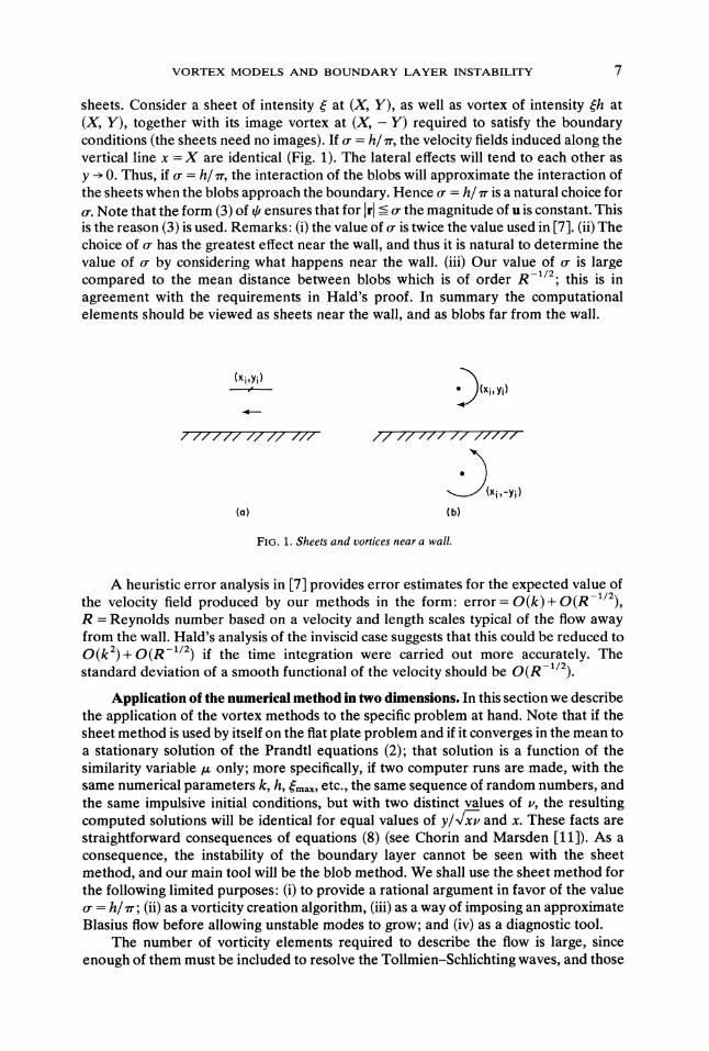
sheets. Consider a sheet of intensity sc at (X, Y), as well as vortex of intensity :h at(X, Y), together with its image vortex at (X, -Y) required to satisfy the boundaryconditions (the sheets need no images). If o" h/zr, the velocity fields induced along thevertical line x X are identical (Fig. 1). The lateral effects will tend to each other asy 0. Thus, if r h/zr, the interaction of the blobs will approximate the interaction ofthe sheets when the blobs approach the boundary. Hence r h/7r is a natural choice forr. Note that the form (3) of ensures that for Irl -< the magnitude of u is constant. Thisis the reason (3) is used. Remarks" (i) the value of r is twice the value used in [7]. (ii) Thechoice of r has the greatest effect near the wall, and thus it is natural to determine thevalue of r by considering what happens near the wall. (iii) Our value of r is largecompared to the mean distance between blobs which is of order R -1/2", this is inagreement with the requirements in Hald’s proof. In summary the computationalelements should be viewed as sheets near the wall, and as blobs far from the wall.

(xi’Yi)" (xi, Yi)

(a)

11 II ill II IIIli

,(xi ,_yi)

(b)

FIG. 1. Sheets and vortices near a wall.

A heuristic error analysis in [7] provides error estimates for the expected value ofthe velocity field produced by our methods in the form" error=O(k)+O(R-1/2),R Reynolds number based on a velocity and length scales typical of the flow awayfrom the wall. Hald’s analysis of the inviscid case suggests that this could be reduced toO(k-)+O(R -1/) if the time integration were carried out more accurately. Thestandard deviation of a smooth functional of the velocity should be O(R-I/).

Application of the numerical method in two dimensions. In this section we describethe application of the vortex methods to the specific problem at hand. Note that if thesheet method is used by itself on the fiat plate problem and if it converges in the mean toa stationary solution of the Prandtl equations (2); that solution is a function of thesimilarity variable/z only; more specifically, if two computer runs are made, with thesame numerical parameters k, h, :max, etc., the same sequence of random numbers, andthe same impulsive initial conditions, but with two distinct values of ,, the resultingcomputed solutions will be identical for equal values of y// and x. These facts arestraightforward consequences of equations (8) (see Chorin and Marsden [11]). As aconsequence, the instability of the boundary layer cannot be seen with the sheetmethod, and our main tool will be the blob method. We shall use the sheet method forthe following limited purposes: (i) to provide a rational argument in favor of the valuer h/zr; (ii) as a vorticity creation algorithm, (iii) as a way of imposing an approximateBlasius flow before allowing unstable modes to grow; and (iv) as a diagnostic tool.

The number of vorticity elements required to describe the flow is large, sinceenough of them must be included to resolve the Tollmien-Schlichting waves, and those


have a short wave length. From linear stability theory (see e.g. [29], [21]) one finds thatthe wave number ot unstable Tollmien-Schlichting waves is between roughly 0.1 /8 and0.4/8 for moderate values of Rs, say very roughly 0.3/8 0.2/x/--xx. The correspondingwave length is 107rx/-xxv; the number of waves between 0 and x is roughly x divided by10rx/x, i.e. -..Rs/50. The first unstable modes occur whenR 500, i.e., one has to beable to resolve at least 10 waves between the leading edge and the first occurrence ofgrowing modes. One can also see that the time period is correspondingly small. For thisreason stability calculations based on the Navier-Stokes equations are very expensiveindeed (see e.g. Fasel [15]).

There is an additional constraint in the present work. It is interesting to comparethe behavior of the growing modes in two dimension with the corresponding behavior inthree dimensions; the two cases are quite different, and the contrast is very instructivewhen one is interested in the transition to turbulence. We wish to use comparablenumerical parameters in two and in three dimensions, so that the comparison of theresults be believable; the cost of three dimensional calculations is of course much largereven than the cost of two dimensional calculations; we must therefore look for ways ofrepresenting the boundary layer which are as economical as possible and yet exhibit acorrect behavior.

There is no obvious way in which the steady Blasius profile can be imposed exactlyon our array of vortex elements at the initial time. On the other hand, a calculationwhich starts from impulsive initial data contains a large and rather long-lived transientcomponent whose behavior is not easily distinguishable from that of a growing mode.Part of this problem can be removed as follows: Start the calculation by using the sheetrepresentation only (which is cheap and allows no instability), and run for a time0 < < To, To large enough so that the Blasius profile will have been reached with somenot unreasonable accuracy. At time To allow some or all of the sheets to becomeblobs. In all the two dimensional runs described below we set To 1.

It is quite obvious that we shall not be able to duplicate the results of linearizedstability theory. The initial data will not coincide exactly with the Blasius solution. Theperturbations will not be small. In Fasel [15] the perturbation amplitude was about 0.05of the free-stream velocity--an impossibly low level for our method. Our results shouldbe compared with the behavior of finite amplitude perturbations in noisy flow. Theadvantages of our numerical method can be seen from the fact that the method requiresno scaling. The very same program can be used to solve an interior flow problem. Thealgorithm provides its own scaling and concentrates the computing effort where it isneeded. This should be particularly important in other problems where thin shear layersoccur at locations which are not known in advance.

In the calculations described below, the vorticity is created at walls in the form ofsheets, with all Iscil-< :max. If the amount of vorticity needed to satisfy the boundaryconditions is less than o, no sheets are created; here, :0 max/2. When sheets findthemselves at y > at time > To, they become blobs; they become sheets again if y < l.must be such that the probability that r/> 2l is small. We checked that as long as

l---1.5 the standard deviation of r/, the results were insensitive to the value of l.Detailed calculations were performed for 0 -< x =< 1; i.e., the typical streamwise length L

-1is 1, and thus R UL/, , Both sheets and blobs were followed for x > 1 butallowed to move only with the random component in their laws of motion. When theyreached x X they were deleted. This was done to ensure that the right boundary atx 1, which is introduced only for computational convenience, behaves as an absorbingboundary and does not affect adversely the calculations in the region of interest0-< x -< 1. We usually picked X 2.


The interaction of two elements at least one of which was a sheet, was computed asif both were sheets. Two blobs interacted as blobs. In the computation of the tangentialvelocity at the wall, all elements were treated as sheets.

After much experimentation we picked :max 0.6. This is a large value of max andproduces a crude and noisy boundary layer; however, it is sufficient for exhibiting themain effects. A relatively large value of :max reduces the number of elements in thecalculation, and, as explained above, this is of particular importance since we intend topresent a three dimensional calculation. The choices of h and k are described in the nextsection.

In the steady state, the drag D(x) on the piece of boundary between 0 and x can becomputed by the momentum defect formula (see e.g. [35]).

(10a) D(x) u(U-u) dy, u u(x, y).

The normalized drag is defined as

(10b) d(x) D(x)/Do(x),

where Do(x) is the Blasius drag Do(x)= 0.6641x/-xx, which can be obtained from theBlasius solution. The velocities for use in formulas such as (10) are computed as if all theelements were sheets. We shall use d(x) defined by (10) as a measure of the amplitude ofthe growing modes even when the flow is not steady and D(x) is not really the drag on[0, x].

Finally, we observed that if k was too large the solution exhibited large oscillationof no possible physical significance. This is readily understood. We are solving amoderately large system of ordinary differential equations by Euler’s method. Theremedy is to reduce k. k <= h is adequate.

Numerical results in two dimensions. In Table 1 and Fig. 2 we display thenormalized "drag" d(x) at X= 1/2 as a function of R and t. (d(X) is the ratioD(X)/Do, see formula (10) above). These calculations were made with k h =0.05;

d 2

o0

I=R: 100,000, Ra: 584rr R=50,O00, Ra=272

/N=I0,000,R=I22

1.5 2 2.5 ;5 5.5

FIG. 2. Growth of an unstable layer in two dimension.


TABLEDrag as a function o[ Reynolds number and time.

R 10000 R 50000 R 100000(R8 122) (R8 272) (R 384)

1.11 1.11 1.111.5 1.23 1.87 1.972 0.89 1.18 1.392.5 1.15 1.44 1.573 .77 1.25 1.65

the other parameters are as described in the preceding section: max=0.6, X 2,r h! r. The pointX 1/2 is in the middle of the region of interest. In our units, , R -1

andR /, 1.72v/R/2. From Table 1 and Fig. 2 one can see that d(X) is growing forR8 394, R 105; d(X) is not growing for R 122, R 104, and d(X) is initiallyexcited but ultimately slowly decaying for R 272, R 5 104. This last fact isdebatable’, the value R 272 seems to be the approximate value of R’c. These resultsare reasonable in view of what is known from the theory and from experiments.

In Fig. 4 we exhibit the edge of the boundary layer as a function of x for 3,R 104. The edge is defined as the smallest value of y for which u U. The edge is notat infinity because we have finite number of vortex elements and thus the tail of theprobability distribution of the locations of the elements is not accurately approximated.The layer is stable at this value of R, yet the edge is ragged and the layer appears to be"intermittent" (for a definition of intermittency see e.g. Cebeci and Smith [4]). The"intermittency" is due to the presence of discrete vortices; this connection will be

A

o R I0,000z R= IO0, O00 Tr Z o

/ o /

0.5U

FIG. 3. Velocity profiles in two dimensions.


2O

0,2 0.4 0.6 0,8 1.0

FIG. 4. Boundary layer shape.

exploited elsewhere for producing models of intermittency. It is obvious from Fig. 4 thatthe wave length of the growing modes cannot be determined directly from theinstantaneous velocity distribution. However, it can be estimated indirectly. Considerthe following question: how small must h be to allow us to distinguish between stableand unstable layers? Suppose that for h > h0 this distinction can be made, but for h =< hothe layer appears to be stable even when it should not be. Then h0 is an estimate of thewave length of the growing modes, since when h <-h0 these modes are suppressed. InTable 2 we present the values of d(X) at X 1/2 as a function of h for R 105. We seethat 10 < h0 < 15, in a reasonable if rough agreement with the Tollmien-Schlichtingtheory.

TABLE 2Drag as a function of h, R 100000, Rs 384.

h=1/20, k=1/201.5 2 2.5 3

d 1.11 1.97 1.39 1.57 1.65

h=1/15, k=1/151.27 2 2.67 3.33

d =0.98 1.48 1.66 1.70

t=l 2 3h=l/lO, k=l/lO =0.98 1.10 1.08

In Fig. 3 we display the velocity as a function of/x y/uatX for R 104 andR 105, averaged over 10 steps between 2.5 at 3. Curve I is the laminar steadyBlasius profile, and curve II was drawn in what appears to the eye as a reasonableneighborhood of the points obtained at R 105. The fluctuations are large (as one maywell expect since max 0.6), but the points at R 104 are in a reasonable agreementwith the Blasius curve; curve II (an unstable case) has a different shape. The gradientsare first sharper, then smaller than in the stable case. This is consistent with experiencein the unstable regime of thermal convection (see e.g. [6]). It is also consistent with datafor a turbulent boundary layer in the following sense: The Tollmien-Schlichting wavesare large scale structures in comparison with boundary layer thickness, while in the


stable regime there are no organized structures. In the turbulent regime one canassociate a velocity with an eddy size; the changes in the profile due to the transitionfrom the stable to the unstable regime should be of the same nature as the changes in thevelocity profile which occur when the eddy size increases. This is indeed the case (seeFavre et al., [16]; their data are reproduced in Lighthill, [28]).

A typical run from 0 to 3 with the numerical parameters used here tookabout 10 minutes on the UC Berkeley CDC 6400 computer. At the end of thecalculation, there were about 200 sheets and 300 blobs.

The physical problem in three space dimensions. We now consider the threedimensional version of the preceding problem.

Consider a semi-infinite flat plate placed on the half plane z 0, x > 0. A fluid ofdensity I occupies the half space z > 0. At time < 0 the fluid is at rest, at 0 the fluid isimpulsively set into motion with velocity U 1. The Navier-Stokes equations in threedimensional space can be written in the form"

(lla) 3,+ (u. V)-(. V)u= R-A,11b) curl u,

(11 c) div u O.

u (u, v, w) is the velocity vector, and r- (x, y, z) is the position vector. The boundaryconditions are(12a) u=(U, 0, 0) for z =o, t>0,

(12b) u=O forz=O,x>O,Ow

(12c) --=0 forz=O,x<O.Oy

Appropriate Prandtl equations can also be written. We shall need below only asimplified version of the equations, as well as the following fact about three dimensionalboundary laminar layer approximations: The vertical component of the vorticityvanishes, i.e., for a solution of the Prandtl equations, - (:1, :2, 0).

The Prandtl equations in three dimensions admit a two dimensional solution, theBlasius solution. That solution is unstable at high enough R. Squire’s theorem (Lin, [29,p. 27]) states that the problem of instability to three dimensional infinitesimal pertur-bation is equivalent to a two dimensional problem at lower R.

Once the two dimensional perturbations begin to grow, several strikingphenomena occur. In particular, before turbulence sets in, streamwise vortices (i.e.vortices whose axis is parallel to the mean flow) make their appearance. Intensesecondary instabilities follow, and spots of intense motion emerge at random locations.An experimental investigation of boundary layer instability can be found in Klebanoffet al. [23]. Experimental investigations of turbulent boundary layers, in whichphenomena resembling those which first arise immediately after the onset of instabilitypersist and may be responsible for some of the observed features, are described e.g. inFavre et al. [16], Kline et al. [24], Willmarth [38]; theoretical aspects of several aspectsof instability are found in Greenspan and Benney [17], Benney [3], Lighthill [28]. Oneof the major conclusions from the experimental data in Klebanoff et al., [23] is that theperturbed flow is periodic in the transverse direction (i.e., y direction). It is thereforenatural to consider in three dimensions equations (11) with the added periodicityconditions

(13) u(x, y +q, z) u(x, y, z), (x, y + q, z) 2(x, y, z),


etc. Furthermore, from Klebanoff et al. (1962) we conclude that q is roughly equal tothe streamwise wave length of the first unstable Tollmien-Schlichting waves; roughly,q 0.1 in our units. We shall therefore be solving equations (11) with the boundaryconditions (12) and (13), and q 0.1.

The numerical methods in three dimensions. We consider first the three dimen-sional analogue of the blob method. The three dimensional problem is more difficultbecause the vorticity is now a stretchable vector quantity which must satisfy div 0.

In earlier three dimensional calculations (Leonard, [26], [27], Del Prete [13],Chorin, (unpublished)), the vorticity field was represented as a sum of vortex filaments.The difficulties with this approach are: (i) a huge amount of bookkeeping is required tokeep track of the changing vortex configurations; (ii) there is no obvious way to generatethe filaments at the boundary in a consistent manner. We bypass these difficulties byrepresenting the vorticity as a sum of vortex segments (Fig. 5). Each vortex segmentmoves in the flow field induced by all the others. The condition div 0 will be satisfiedonly approximately. The segments have no independent physical significance. The twodimensional blobs do not have one either; physical vortices or vortex tubes are expectedto emerge from the superposition of the computational blobs or segments. A segment Ais defined by seven quantities" The coordinates r1) (x 1), y), z)) of the center of itsbase, the coordinates r2) (x 2), Y 2), z 2)) of the center of its top, and its intensity K. Weshall write Ai--(X (1) y) ), X2), y2), 2),z z K), 1 , N, N number of segments.The base and the top are circles of radius tr, (the cut-off), which will be determinedbelow.

Given a vorticity yield (r), the velocity field in a fluid which fills out the wholespace is given by the Biot-Savart formula (see e.g. [2]):

(14)

1 I a (r’)u(r)

4r a3 dr’

If the vorticity field is a sum of N closed vortex lines with the ith line havingintensity ri, (14) becomes

(15) u(r)1 I as

t(’i 3 ds.4r th line a

s s(r’) is the unit tangent vector to the ith line at r’, ds ds(r’) is the arc length along theith line, and as before a =r-r’. We now seek an interaction law between vortexsegments which will approximate the motion induced by (14) or (15).

FIG. 5. A vortex segment.


Inside the segment the velocity field must be kept bounded, just as is the case in twodimension. Furthermore, the field must be modified inside the segments in such a waythat the segments will be compatible with the boundary calculations (see below). Theproblem of the finding the correct formulation of the vortex method in three dimensionsis difficult, (see e.g. Leonard [27]). The formulation offered here is plausible but notrigorously justified.

We require that the motion of a vortex ring or line made up of vortex segmentsshould preserve the shape of the ring or line. This can be accomplished by ensuring thatthe configuration of the vectors a and of the velocity vectors which enter the formula forthe motion of the tips of the segment is the appropriate translate of the correspondingconfigurations which determine the motion of the bases. Thus, let Ai, A be two vortexsegments; define

.(1) (X(1) (1) (1) _(2) (2) (2) 12)Yi ,Zi ), --(X YiI’i Z )7_(2) _(1)

$i ri ri_(1) _(1) _(1) _(2) _(2)_r2) with aii la etc.klij r --r klij r

The velocity fields GI), ..,,!?) induced by A. at r and r will be approximated by"(2) :>(1) > and aIf aii ---o" --o"

(1)

,(1)(16a) ,,...,.i] err (a(1))3’ii

(2)

(16b) !?)"’ 4rr (a (2))3

(1) (1)If either a0

-r’a !.1)__ a s.0.2 (1)"" 4 a i]

(17b) i] 4 a(

The equations of motion for each segment can now be obtained by summing thecontributions of all the other segments and then adding to that sum the appropriaterandom component. This yields

(1)n+l 1.l)n(18a) ri + k E -"i] "’’q,]#i

(18b) _(2)n+l _(2)n i!.2)ri =ri +k Y’. +1,l]]1

where rll)’--= ri(X)(nk), etc., and is a vector 1 (r/, ’12, r/3), with T/l, r/2, */3, Gaussianrandom variable with means 0 and variances 2k/R, independent of each other. q in(18a) is identical to 1 in (18b), since diffusion does not introduce rotation or stretching.The boundary condition at the wall can be satisfied as before by the introduction ofappropriate image segments.

One can write the boundary layer equation in three dimensions and solve them by amethod in which the computational elements are pieces of a vortex sheet (--"tiles")with sides h in the x direction and h2 in the y direction. Each tile carries a twodimensional vortex with components q, :2. As observed earlier, 3 0 in the boundarylayer equations. However, we shall use the tiles only near the boundary, where vortex


stretching is presumably negligible, or to create an initial Blasius profile, in whichstretching is exactly zero. Therefore, the boundary layer equations we shall be solvingreduce to

021 02Z2c3t: - (11" V):I b’ 2, Ot2 -Jr- (11" V):2 / 2

Oz Oz

OV c3udiv u 0, u (u, v, w).

These equations can be solved by a straightforward extension of the sheet methoddescribed earlier. No vortex stretching will be taken into account, and we shall not takethe trouble to write out the equations in full. The rejection and variance reductiontechniques carry over from the two-dimensional case. Care is taken to ensure that

4’21’’’’’- 22 :max.A tile created near the wall can become a segment if > T or if zi > I. A segment

which falls below becomes a tile again. The transformation of tiles into segments (andvice versa) must obey the following conditions:

(i) A tile must become a segment parallel to the wall; i.e., if a tile (Xi, Yi, Zi, li, 2i)(1) (1) 12), (2) _(2) /i) we must havebecomes a segment (xl1, Yi Zi X Yi zi

(19a) zl2 -zl2 =0.

(ii) A flow which is two dimensional when described by tiles must remain twodimensional when described by segments. The two dimensionality of a flow describedby segments will be preserved only if the flow fields seen by the tips of the segments aretranslates of the flow fields seen by the bases, with a translation vector normal to theplane of the flow and pointing in the direction of a fixed normal n to that plane.

(iii) The stretching of the several segments represents the stretching of vorticity,which will be represented accurately only if the length of the segments is reasonablysmall. A reasonable normalization of that length in our problem is

(19b) y12) yl) h2 when a segment is created.

(iv) The circulation around a vortex line made up of tiles must equal the circulationaround a vortex line made up of segments. If y2)--Yi is normalized by (19b) thisrequirement leads to

(19c) Ki hlx/sc + :i sgn (’. n),

where t’ (SCl, sc2), n is the fixed normal to the plane of the flow and sgn(c) 1 if c => 0,sgn(c) 1 if c < 0.

The remaining connecting formulas between segments and tiles are obviously(1)(19d) xi =xi,

(19e) yl1 =yi,

(1)(19f) z zi.

Formulas (19) are of course invertible, and the computational elements can be treatedas either tiles or segments, as the occasion warrants.

When two segments interact, their interaction is given by formulas (19); when asegment and a tile interact, they are both viewed as tiles.

Finally, the cut-off must be determined. We must require that if we consider on onehand the interaction of two infinite vortex lines parallel to the y axis represented by


segments, and on the other hand the interaction of the same vortex lines represented bytiles, the former should approach the latter as the lines approach the wall. Thisrequirement obviously reduces to the condition imposed on r in two dimensions, andyields r hl!’rr. This conclusion is of course legitimate only if most of the vorticity doesindeed point in a direction parallel to the y axis.

Application of the numerical methods in three dimensions. In this section wediscuss some of the features of the numerical method which are specific to the particularapplication at hand. Most of the numerical parameters are chosen just as they werechosen in the two-dimensional case; in particular, and L. We picked h k 5, sincethe two-dimensional calculations showed that this was a minimal but adequate choice.We picked h2 q/4, after some experimentation showed that this value was sufficient toexhibit important effects.

The two major difficulties we encountered in three dimensions were: the largeamount of computational labor, and the difficulty in imposing periodic boundaryconditions on a grid-free method. The amount of labor is large not only becausethree-dimensional calculations are always more costly than two-dimensional cal-culations, but also (and especially) because the specific nature of the secondaryinstabilities which arise in three dimensions (see the next section) requires the creationof large amounts of vorticity at the walls. In consequence we used max 1. This valueseems to yield results which are compatible with two-dimensional results obtained withsmaller values of max, but it is obviously so large that one may legitimately argue thatwhat we have is a model rather than an approximation.

Periodic boundary conditions can be imposed on a vortex calculation, but the pricein computing labor is high. There again we did the least we could reasonably do. Foreach vortex segment with base located at (x, y, z) (or its image created to satisfy thenormal boundary condition, with a base at (x, y,-z)) we created two more segments,based at (x, y 4- q, z), q the period and took their velocity fields into account when wemoved the segment. Similarly, new tiles must be created outside the strip 0 =< y -< q withlocations and strengths determined by periodicity. Some rather complex programmingis needed to keep track of the several image systems as the tiles become segments andvice versa.

Finally, we note that if 1 0 at 0, i.e., if there is no streamwise vorticity at all at0, none will ever be created by our algorithm. Thus, if we are to observe the effects of

streamwise vorticity, we must introduce some by artificial means. We proceeded asfollows: At =0, for one time step, we changed the velocity at infinity. Instead ofu(x, y, oo)= (U, O, O) we set

Numerical results in three dimensions. Calculations done in three dimensions withA 0 (i.e. with no perturbation which could trigger three dimensional effects) produceresults similar to the results of two dimensional calculations. They afford a check onboth, but are not worth discussing separately.

u(x, y, oo) =(uoo,( A, 0)

(Uoo, 0, 0) elsewhere.

We usually picked A 10-3 (note that U 1). For > k, we reverted to u(x, y, oo)=(Uoo, 0, 0) everywhere. The effect of this initial perturbation is to create a smallstreamwise vortex at the boundary, whose subsequent history is determined bydiffusion, transport, and stretching.


FIG. 6. Amplification of streamwise rotation.

Even a very small value of A (i.e. a very small three dimensional perturbation) hasa substantial effect at all values of R we tried. The first phenomenon one observes whenA # 0 is that the boundary layer becomes thicker than in the case A 0. The mechanicsof this effect are somewhat complex. A reasonable qualitative explanation is as follows:the rotation whose axis is parallel to the flow induces the creation of new streamwisevorticity at the wall. The new vorticity is then collected in streamwise strips in which theflow induced by the streamwise vortex leads away from the wall, while the regionswhere the induced flow points to the wall are depleted (see Fig. 6). The part of theboundary layer which thus expands can expand substantially, while the part whichcontracts cannot contract below zero. As a result the computed boundary layerthickness 8 increases; at (X, Y) is defined by

| (1-u(x, y, )/U) dt.J0

In Figs. 7 and 8 we plot the ratio 8/b where =computed boundary layerthickness at X 1/2 averaged over a period in y, and b boundary layer thickness atX 1/2 computed from the steady Blasius solution. In Fig. 7, R 20000. Note that at

3, R8 computed with the steady is R8 187, and thus the layer should be steady.However, if R is evaluated with the computed boundary layer thickness, R atX 1/2 isapproximately 300, andR at X 1 is approximately 440, well over the value at whichthe layer becomes unstable in the two-dimensional calculation. In Fig. 8, R 100000,

R:20,O00 5D

\

2D

0.5 .5 2 2.5 :

FIG. 7. Growth o[ boundary layer thickness, R 20000.


R=IO0,O005D

0.5 1.5 2 2.5 5

FIG. 8. Growth ot boundary layer thickness, R 100000.

and the same effect is reproduced. The computed values of the drag are not greatlyaffected by this thickening of the layer. (This is quite plausible, in view of the extra factoru in the integrand in the formula for the drag; the effect of this factor is to reduce thedependence of the drag on the velocity profile near the wall.)

When the layer becomes unstable to Tollmien-Schlichting waves, the streamwisevorticity begins to grow. The possible mechanisms for this growth are well known" Thewaves stretch lines; furthermore, they can create situations in which a horizontalstreamwise line tilts away from the horizontal; its higher parts move faster than thelower parts, and stretching results. All segments are initially created with length h2. Ifthey stretch their length becomes 11"12)- 1’I1) I. The ratio g Ir2- rl[/h2 is the stretchingratio. In Figs. 8 and 9 we plot , the average value of g, averaged over all segments. It is

R=200,O00

o0 2 5

FIG. 9. Amplification of boundary layer disturbances in three dimensions, R 20000.


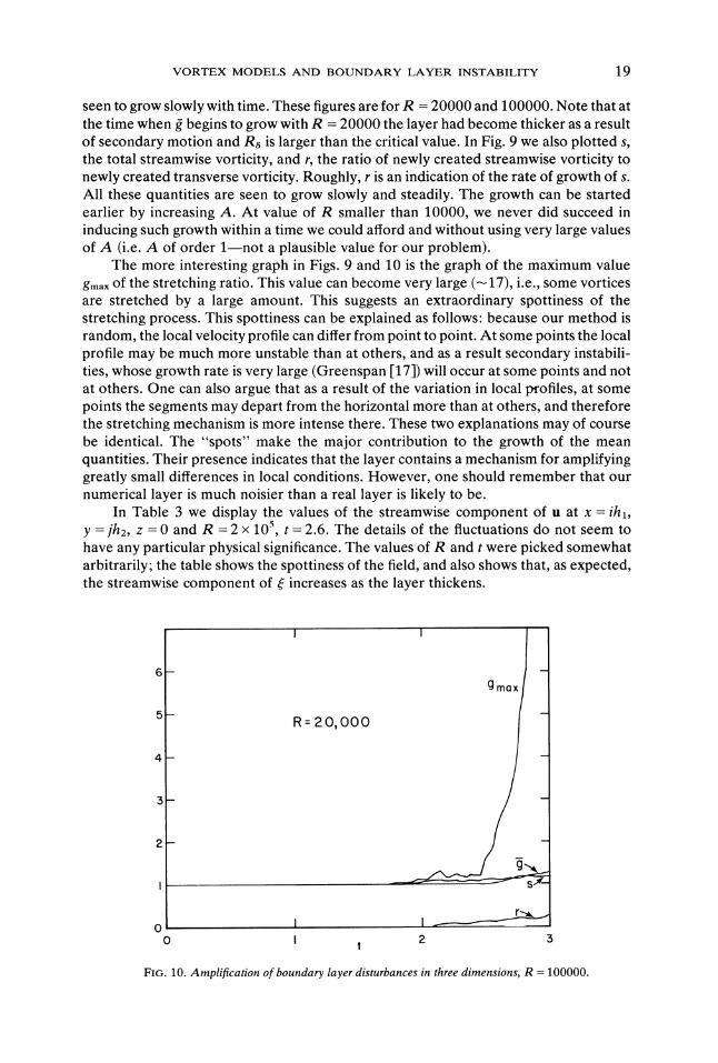
seen to grow slowly with time. These figures are for R 20000 and 100000. Note that atthe time when g begins to grow with R 20000 the layer had become thicker as a resultof secondary motion and R is larger than the critical value. In Fig. 9 we also plotted s,the total streamwise vorticity, and r, the ratio of newly created streamwise vorticity tonewly created transverse vorticity. Roughly, r is an indication of the rate of growth of s.All these quantities are seen to grow slowly and steadily. The growth can be startedearlier by increasing A. At value of R smaller than 10000, we never did succeed ininducing such growth within a time we could afford and without using very large valuesof A (i.e. A of order lmnot a plausible value for our problem).

The more interesting graph in Figs. 9 and 10 is the graph of the maximum valuegmax Of the stretching ratio. This value can become very large (---17), i.e., some vorticesare stretched by a large amount. This suggests an extraordinary spottiness of thestretching process. This spottiness can be explained as follows: because our method israndom, the local velocity profile can differ from point to point. At some points the localprofile may be much more unstable than at others, and as a result secondary instabili-ties, whose growth rate is very large (Greenspan [17]) will occur at some points and notat others. One can also argue that as a result of the variation in local profiles, at somepoints the segments may depart from the horizontal more than at others, and thereforethe stretching mechanism is more intense there. These two explanations may of coursebe identical. The "spots" make the major contribution to the growth of the meanquantities. Their presence indicates that the layer contains a mechanism for amplifyinggreatly small differences in local conditions. However, one should remember that ournumerical layer is much noisier than a real layer is likely to be.

In Table 3 we display the values of the streamwise component of u at x ihl,y =/’h2, z 0 and R 2 105, 2.6. The details of the fluctuations do not seem tohave any particular physical significance. The values of R and were picked somewhatarbitrarily; the table shows the spottiness of the field, and also shows that, as expected,the streamwise component of increases as the layer thickens.

R 2 O, O00

g m

0 2 3

FIG. 10. Amplification of boundary layer disturbances in three dimensions, R 100000.


When g increases, more and more segments and tiles have to be created; this is whywe needed a large value of max. A further consequence is that computing for largertimes than what we displayed is more expensive than we could afford. A typical run for0 <-t <-3 took about one hour of CDC 6400 time at Berkeley.

TABLE 3Streamwise vorticity at the boundary, R 2 x 105, 2.6

i= 1 2 3 4

i= 1 .000 .000 .000 -.0012 .000 .000 .000 .0003 .000 .000 .000 .0004 .003 .000 .000 .0005 .028 .000 .001 .0006 .000 .000 .000 .0017 -.046 -.012 .001 .0018 -.046 -.004 -.008 -.0109 -.038 -.028 -.002 -.244

10 -.187 -.054 -.007 -.09311 .091 -.065 .030 .07612 -.062 -.310 .136 .20513 2.260 .507 .480 1.07014 -.077 .150 .826 -.62115 -.552 .422 .001 -.273

12ondusions. Our vortex methods, including the new three dimensional versionand the new vorticity creation procedure, seem to be able to reproduce importantfeatures of boundary layer behavior in two and three dimensions and at Reynoldsnumbers where instability is expected. The three-dimensional calculation does exhibit agrowth of streamwise vorticity as well as spottiness; however, it was not performed fortimes long enough tor anything resembling fully developed turbulence to be present.Unlike other methods, our methods are not limited at high R by the difficulty indistinguishing real from numerical diffusion; they are however limited, like othermethods, by the fact that effects not resolved cannot be seen; i.e., if there are not enoughcomputational elements to represent a phenomenon, that phenomenon will not beobserved. Since tully turbulent flow is very complicated, our methods do not remove theneed for careful modeling in some practical applications.

REFERENCES

[1] W. ASHURST, Numerical simulation ofturbulent mixing layer dynamics, SANDIA (Livermore) Report(1977).

[2] G. K. BATCHELOR, An Introduction to Fluid Mechanics, Cambridge University Press, London, 1967.[3] D. J. BENNEY, A nonlinear theory for oscillations in a parallel flow, J. Fluid Mech., 10 (1960), p. 209.[4] T. CEBECI AND A. M. O. SMITH, Analysis o[ TurbulentBoundary Layers, Academic Press, New York,

1974.[5] A. CHEER, Program BOUNDL, LBL-6443 Suppl. Report, Lawrence Berkeley Lab. (1978).[6] A.J. CHORIN, A numerical method[or solving incompressibleflow problems, J. Comput. Physics, (1967),

p. 12.[7] ., Numerical study ofslightly viscous flow, J. Fluid Mech., 57 (1973), p. 785.[8] ., Gaussian fields and random flow, Ibid., 63 (1974), p. 21.[9] ., Lectures on Turbulence Theory, Publish/Perish, Boston (1976).

[10] ., Vortex sheet approximation of boundary layers, J. Comput. Physics, 27 (1978), 428.


11 A.J. CHORIN AND J. E. MARSDEN, A MathematicalIntroduction to FluidMechanics, Springer Verlag,New York, 1979.

[12] A. J. CHORIN, T. J. R. HUGHES, M. F. MCCRACKEN AND J. E. MARSDEN, Product formulas andnumerical algorithms, Comm. Pure Appl. Math., 31 (1978), p. 205.

[13] V. DEE PRETE, Numerical simulation o/" vortex breakdown, LBL Math. & Comp. Report 1978.[14] W. ECKHAUS, Studies in Nonlinear Stability Theory, Springer Verlag, New York, 1965.15] H. FASEL, Investigation of the stability ofboundary layers in a finite difference model ofthe Navier-Stokes

equations, J. Fluid Mech., 78 (1970), p. 355.[16] A. FAVRE, J. GARIGLIO AND J. DUMAS, Phys. Fluids, 12, Suppl. (1967), p. 138.[17] H. P. GREENSPAN AND D. J. BENNEY, On shear layer instability, breakdown and transition, J. Fluid

Mech., 15 (1963), p. 133.[18] O. HALD, The convergence of vortex methods II, SIAM J. Numer. Anal., 16 (1979), p. 726.[19] O. HALD AND V. DEE PRETE, The convergence o.fvortex methods, Math. Comp., 32 (1978), p. 791.[20] J. M. HAMMERSLEY AND D. C. HANDSCOMB, Monte Carlo Methods, Methuen, 1964.[21] R. JORDINSON, Theflat boundary layer, PartI. Numerical integration ofthe Orr-$ommerfeld equation, J.

Fluid Mech., 43 (1970), p. 801.[22] H. T. KIM, S. J. KLINE AND W. C. REYNOLDS, The production o.f turbulence near a smooth wall in a

turbulent boundary layer, Ibid., 50 (1971), p. 133.[23] P. S. KLEBANOFF, K. O. TIDSTROM AND L. O. SARGENT, The three dimensional nature ofboundary

layer instability, Ibid., 12 (1962), p. 1.[24] S.J. KLINE, W. C. REYNOLDS, F. A. SCHRAUB AND P. W. RUNDSTADLER, The structure ofturbulent

boundary layers, Ibid., 30 (1967), p. 741.[25] J. LAMPERTI, Probability Theory, Benjamin, New York, 1966.[26] A. LEONARD, Numerical simulation of interacting, three dimensional vortex filaments, Proc. 4th Int.

Conf. Num. Methods Fluid Dynamics, Springer Verlag, New York, 1975.[27] ., Simulation of unsteady three dimensional separated flows with interacting vortex filaments, Proc.

5th Int. Conf. Num. Mech. Fluid Dynamics, Springer Verlag, New York, 1977.[28] M. J. LIGHTHLL, Turbulence, Osborne Reynolds and Engineering Science Today, Manchester Univ.

Press, 1976.[29] C. C. LIN, The Theory o]’ Hydrodynamic Stability, Cambridge University Press, London, 1966.[30] M. F. MCCRACKEN AND C. S. PESKIN, The vortex method applied to blood flow through heart valves,

Proc. 6th Int. Conf. Num. Methods Fluid Dynamics, Springer Verlag, New York, 1978.[31] D. MEKSYN AND J. T. STUART, Nonlinear instability, Proc. Roy. Soc. London, A, 208 (1951), p. 517.[32] L. ONSAGER, Statistical hydrodynamics, Nuovo Cimento, 6, Suppl. (1949), p. 229.[33] E. RESHOTKO, Boundary layer stability and transition, Ann. Rev. Fluid Mech., 8 (1976), p. 311.[34] H. L. ROGLERAND E. RESHOTKO, Disturbances in a boundary layerintroduced by a low intensity array

of vortices, SIAM J. Appl. Math., 28 (1975), p. 431.[35] H. SCHLICHTNG, Boundary Layer Theory, McGraw-Hill, New York, 1960.[36] A.I. SHESTAKOV, A hybrid vortex--ADIsolutionforflows oflow viscosity, J. Comput. Phys., 31 (1979),

p. 313.[37] A. A. TOWNSEND, Boundary LayerResearch, Freiburg Symposium, H. Gortler, Ed., Springer Verlag,

1958.[38] W. W. WILLMARTH, Structure oiturbulence in boundary layers, Advances in Appl. Mech., 15 (1976), p.

159.

Voi. VORTEX MODELS AND INSTABILITY* - UCB ...chorin/C80.pdfVoi. 1, No. 1, March1980 (C)...

Documents

Transcript of Voi. VORTEX MODELS AND INSTABILITY* - UCB ...chorin/C80.pdfVoi. 1, No. 1, March1980 (C)...