HAL Id: tel-01801769https://tel.archives-ouvertes.fr/tel-01801769

Submitted on 28 May 2018

HAL is a multi-disciplinary open accessarchive for the deposit and dissemination of sci-entific research documents, whether they are pub-lished or not. The documents may come fromteaching and research institutions in France orabroad, or from public or private research centers.

L’archive ouverte pluridisciplinaire HAL, estdestinée au dépôt et à la diffusion de documentsscientifiques de niveau recherche, publiés ou non,émanant des établissements d’enseignement et derecherche français ou étrangers, des laboratoirespublics ou privés.

VMS data analyses and modeling for the monitoring andsurveillance of Indonesian fisheries

Marza Ihsan Marzuki

To cite this version:Marza Ihsan Marzuki. VMS data analyses and modeling for the monitoring and surveillance of In-donesian fisheries. Computer Vision and Pattern Recognition [cs.CV]. Ecole nationale supérieureMines-Télécom Atlantique, 2017. English. �NNT : 2017IMTA0012�. �tel-01801769�

THÈSE / IMT Atlantique

sous le sceau de l’Université Bretagne Loire

pour obtenir le grade de

DOCTEUR D'IMT Atlantique

Mention : Sciences et Technologies de l’Information et de la Communication

École Doctorale Sicma

Présentée par

Marza Ihsan Marzuki Préparée dans le département Signal et communication

Laboratoire Labsticc

Analyse et modélisation

des données VMS pour

le suivi et la surveillance

des pêches indonésiennes

VMS data analyses and

modeling for the monitoring

and surveillance of

Indonesian fisheries

Thèse soutenue le 27 mars 2017

devant le jury composé de :

Nicolas Bez Chercheur, IRD Centre de Recherche Halieutique / président Sophie Bertrand Chargée de recherches (HDR), IRD Centre de Recherche Halieutique / rapporteur

Stéphanie Mahévas Chercheur (HDR), IDR Ifremer / rapporteur

René Garello Professeur, IMT Atlantique / examinateur

Ronan Fablet Professeur, IMT Atlantique / directeur de thèse

Vincent Kerbaol Directeur, CLS-Plouzané / invité Philippe Gaspar Coordinateur scientifique, CLS-Toulouse / invité

i

Acknowledgments

First and foremost I would like to thank my supervisor Professor Ronan Fablet. It has been an honor and pleasure working with him. His valuable advices, dynamism, sincerity and support during this thesis allowed me to obtain new knowledges and extend my experiences. He was not only an advisor and tremendous mentor but also a good friend. Thank you for your guidance, it has been a true pleasure and I hope that we could continue our collaboration. I am also grateful to my co-supervisor Dr. Philippe Gaspar and Professor René Garello. Their wide knowledges and logical way of thinking have been of great value for me. I would like to thank the committee members. I thank Dr. Sophie Bertrand and Dr. Stéphanie Mahévas for accepting being my thesis reviewers and for their attention and thoughtful comments for improving the quality of my dissertation. I thank Dr. Nicolas Bez for accepting to carry out the task of the committee president and Dr. Vincent Kerbaol for being my thesis examiners. Your insightful comments and encouragement incented me to widen my research from various perspectives. I owe my deepest gratitude to the members of the Signal and Communication department to give me a chance for studying in your laboratory. I would like to thank Dr. Pierre Tandeo, Dr. Pierre Ailliot and Dr. Rocio Joo for their kind help and assistance. A special thank you to all my office mates that not I mention here individually. You are all always in my heart. I gratefully acknowledge the financial support from the Ministry of Marine Affairs and Fisheries through the project INDESO that make this PhD possible. My sincere thanks goes to all my colleagues in Agency for Marine and Fisheries Research & HRD to support my PhD pursuit. Also a big thank you to all CLS team and capacity building members under INDESO Project for your time and effort in supporting data and solutions. And last but not least, I am forever thankful to my family: my father, my mother, my sisters and my brother who always support me with help, understanding and pray. I express my deepest gratitude to my loving wife and children. Their love, encouragement, and moral support have made me to pass through many difficult times. I dedicate this thesis to all of you, my wonderful family.

ii

Abstract

Monitoring, control and surveillance (MCS) of marine fisheries are critical issues for the sustainable management of marine fisheries. In this thesis we investigate the space-based monitoring of fishing vessel activities using Vessel Monitoring System (VMS) trajectory data in the context of INDESO project (2013-2017). Our general objective is to develop a processing chain of VMS data in order to: i) perform a follow-up of the fishing effort of the Indonesian longline fleets, ii) detect illegal fishing activities and assess their importance. The proposed approach relies on classical latent class models, namely Gaussian Mixture Models (GMM) and Hidden Markov Models (HMM), with a view to identifying elementary fishing vessel behaviors, such as travelling, searching and fishing activities, in a unsupervised framework. Following state-of-the-art approaches, we consider different parameterizations of these models with a specific focus on Indonesian longliners, for which we can benefit from at-sea observers’ data to proceed to a quantitative evaluation. We then exploit these statistical models for two different objectives: a) the discrimination of different fishing fleets from fishing vessel trajectories and the application to the detection and assessment of illegal fishing activities, b) the assessment of a spatialized fishing effort from VMS data. We report good recognition rate (about 97%) for the former task and our experiments support the potential for an operational exploration of the proposed approach. Due to limited at-sea observers’ data, only preliminary analyses could be carried out for the proposed VMS-derived fishing effort. Beyond potential methodological developments, this thesis emphasizes the importance of high-quality and representative at-sea observer data for further developing the exploitation of VMS data both for research and operational issues. Key words: Space-based monitoring of fishing vessel activities; fishing effort; illegal fishing; VMS trajectory data; data mining; unsupervised and supervised learning.

iii

Résumé

Le suivi, le contrôle et la surveillance (MCS) des pêches marin sont des problèmes essentiels pour la gestion durable des ressources halieutiques. Dans cette thèse, nous étudions le suivi spatial des activités des navires de pêche en utilisant les données de trajectoire du système de surveillance des navires (VMS) dans le cadre du projet INDESO (2013-2017). Notre objectif général est de développer une chaîne de traitement des données VMS afin de: i) effectuer un suivi de l'effort de pêche des flottilles de palangriers indonésiens, ii) détecter les activités de pêche illégales et évaluer leur importance. L'approche proposée repose sur des modèles de mélange gaussien (GMM) et les modèles de Markov cachés (HMM), en vue d'identifier les comportements élémentaires des navires de pêche, tels que les voyages, la recherche et les activités de pêche, dans un cadre non supervisé. Nous considérons différentes paramétrisations de ces modèles avec une étude particulière des palangriers indonésiens, pour lesquels nous pouvons bénéficier de données d'observateurs embarqués afin de procéder à une évaluation quantitative des modèles proposés et testés. Nous exploitons ensuite ces modèles statistiques pour deux objectifs différents: a) la discrimination des différents flottilles de pêche à partir des trajectoires des navires de pêche et l'application à la détection et à l'évaluation des activités de pêche illégale, b) l'évaluation d'un effort de pêche spatialisé à partir des données VMS. Nous obtenons de très bons taux de reconnaissance (environ 97%) pour la première tâche et nos expériences soutiennent le potentiel d'une exploration opérationnelle de l'approche proposée. En raison du nombre limité de données d'observateurs embarqués, seules des analyses préliminaires on pu être effectuées pour l'estimation de l'effort de pêche à partir des données VMS. Au-delà des développements méthodologiques potentiels, cette thèse met l'accent sur l'importance de la qualité de données d'observation en mer représentatives pour développer davantage l'exploitation des données VMS tant pour la recherche que pour les questions opérationnelles. Mots-clés : Surveillance spatiale des activités des navires de pêche; l'effort de pêche; la pêche illégale; les données de trajectoire; VMS l'extraction de données; l'apprentissage non supervisé et supervisé.

iv

List of figures Chapter Fig. Description Page

1 1 The trend of world marine fisheries 1

2

1 Indonesian production in capture fisheries comparing with worldwide capture fisheries 7

2 Comparison among major commodities in Indonesian marine capture fisheries 8

3 Fisheries Management Area (FMA) in Indonesia 12 4 Number of fishing vessels from VMS data in this study 19

5 Number of VMS data (ping records) for: (a) longline fishing vessels, (b) purse-seine fishing vessels, (c) pole-and-line fishing vessels, (d) shrimp trawl fishing vessels

21

6 Number of fishing vessels from observer data that considered in this study 22

7

Track of fishing vessel that show fishing activities from VMS data (dark blue: non fishing; green: fishing) correlated with observer data (red: setting; yellow: hauling), a, b, c, d, e: for longliners

25

8

Track of fishing vessel that show fishing activities from VMS data (dark blue: non fishing; green: fishing) correlated with observer data (red: setting; yellow: hauling), f, g, h, i: for purse-seiners

27

9 Example of position mismatch between VMS track (dark blue: non fishing; green: fishing) and observer data (red: setting, yellow: hauling) for longliners

27

3

1 Number of longline vessels installed VMS device in 2012-2014 40

2 Number of VMS data (ping records) from longline vessels that considered as our dataset 40

3

The comparison of accuracy rate between vessel speed calculated (VSC) and vessel speed instantaneous (VSI) using vessel specific model (VSM) based HMM and global model (GM) based HMM. VSC showed better results for both the VSM model and the GM one. See Section 3.2.3 for details on the differences between VSM and GM models.

42

4 Variables input Vp and Vt 45 5 Graphical state HMM 46

6 Schematic of segment model to consider the characterization behavior of movement ecology hence might improve the performance of model developed.

53

v

7 Activity-dependent distributions of vessel speed for 3 of the considered vessels showing a good consistency across vessels: ((a). vessel A, (b). vessel B, (c) vessel C).

55

8 Activity-dependent daily distributions of each activity for 3 of the considered vessels showing a good consistency across vessels:(a).vessel A, (b). vessel B, (c) vessel C.

57

9

Activity-dependent distributions of the speed and the time of each vessel activity for 3 of the considered vessels showing a poor consistency across vessels: (a). vessel D, (b). vessel E, (c) vessel F.

58

4

1

Comparison of longliners’ fishing effort distribution using global and vessel-specific HMM parameterizations in February-March 2012. (a) raw mapping issued from the global parameterization (Eq. 1); (b) smoothed version of the distribution shown in (a) using a Laplacian diffusion; (c) raw mapping issued from vessel-specific parameterizations (Eq. 1); (d) smoothed version of the distribution shown in (c) using a Laplacian diffusion. See Section II for details on the different models.

75

2

Comparison of longliners’ fishing effort distribution using global and vessel-specific HMM parameterizations in June- July 2014. (a) raw mapping issued from the global parameterization (Eq. 1); (b) smoothed version of the distribution shown in (a) using a Laplacian diffusion; (c) raw mapping issued from vessel-specific parameterizations (Eq. 1); (d) smoothed version of the distribution shown in (c) using a Laplacian diffusion. See Section II for details on the different models.

76

3 The comparison of longliners fishing effort distribution using vessel-specific (VSM) parameterizations (a) and Simple Speed Filter (SSF) parameterization (b) in June- July 2014

77

4

The distribution of longliner activities with grid 1/12° from February to March 2012 (a) for only 2 activities i.e. setting, and hauling; (b) for all activities i.e. setting, hauling and others

78

5 The aggregate of setting-hauling activities between global HMM model (GM) and vessel-specific HMM model (VSM) generated bimonthly for years 2012-2014.

79

6

Average seasonally VMS-based prediction of longliner fishing effort distribution for years 2012-2014. (a) rainy season (NWM, Dec-Mar); (b) transition season (TS-I, Apr-May and TS-II, Oct-Nov); (c) dry season (SEM, Jun-Sep)

82

7 Longline fishing effort distribution for one year period. Red rectangle showed the highest area continually explored each year. (a) 2012; (b) 2013; (c) 2014.

83

8

Comparison of the VMS-derived longliners’ fishing effort index (left side) and SEAPODYM fishing ground prediction for big eye tuna (BET) (right side) for different weekly periods.

84

9 Comparison of the VMS-derived longliners’ fishing effort 85

vi

index (left side) and SEAPODYM fishing ground prediction for yellow fin tuna (YFT) (right side) for different weekly periods.

5

1 Examples of VMS trajectories of Indonesian fisheries for the four fishing gears considered in this study. 97

2

Joint distribution of VMS-derived turning angles and speeds for the considered gear-specific Indonesian fisheries: namely,(a) shrimp trawler, (b) longliner, (c) pole-and-liner, (d) purse-seiner.

98

3

Segmentation of the fishing regimes along a VMS trajectory using different mixture models for speed and turning angle variables with time period of three months: (a) using GvMMM , (b) using GMM-VpVt. Visually, GMM-VpVt model showed better segmentation results for the initial and final segments from and to port, as stressed by likely misclassified steaming activities in subfigure (a) highlighted by red circles. See Section III for details on the different models.

108

4

Distribution of the misclassification rates of the fishing vessels over the entire dataset for repeated 5-fold cross-validation experiments: from multiple cross-validation experiments, we compute for each fishing vessel the misclassification rate as the percentage of misclassification of a fishing vessel when it belongs to the test dataset. We compute the distribution of these misclassification rates over the entire dataset of 1 227 fishing vessels. We only depict the distribution of the non-null misclassification rates, which comprise 47 fishing vessels (misclassification rate=0 (i.e., never misclassified), misclassification rate=100 (i.e., always misclassified)).

109

5

Examples of VMS trajectories associated with a high misclassification rate (above 50 %): (a) longliner misclassified as a purse-seiner, (b) purse-seiner misclassified as a longliner, (c) shrimp-trawler misclassified as a longliner, and (d) pole-and-line misclassified as a purse seiner.

112

vii

List of tables

Chapter Table Description Page

2

1 The production of other fishes in 2014 (see violet color in Fig. 2) 9 2 Capture fisheries production in Indonesia 10 3 Number of fishers in Indonesia 10 4 Number of fishing vessels in Indonesia 10

5 Number of fishing vessel with variance of fishing vessel gear type > 30 GT 11

6 Marine capture fisheries based on FMA (Fisheries Management Area) 12

7 Annual tuna catch by species and gear type 14

8 The number of vessels that could be used for validation historically 23

3

1 Speed characteristic to differentiated longliners' fishing vessel activities 44

2 Mean correlation coefficient at different time steps between successive speed values (Vp and Vt) 45

3 Classification accuracy of the considered models for the prediction of longliners' activities from VMS trajectories 53

4 Classification accuracy of the HMM method for the considered segmental analysis at different time-scale for the entire dataset (6 vessels)

59

5 Classification accuracy of the HMM method for the considered segmental analysis at different time-scale for the partial dataset (3 vessels with a good accross-vessel consistency)

59

6 Relationships between observers’ states and HMM states for the entire dataset (6 vessels) 59

7 Relationships between observers’ states and HMM states for the entire dataset (3 vessels with a good across-vessel consistency) 59

8 Relationships between observers’ states and HMM states for the entire dataset (6 vessels) considering only HMM state segment lasting more than 6 hours.

59

9 Relationships between observers’ states and HMM states for a partial dataset (3 vessels with a good accross-vessel consistency) considering only HMM state segment lasting more than 6 hours.

60

4 1 Correlation Coefficient between Tuna Model (BET) and longline-VMS Model 81

5 1 Comparison of different vms-based features: we report mean correct classification rates over the four fishing gears using a 107

viii

SVM classifier. we consider four feature types, feature types I and II being derived for a GMM-VpVt model.

2 Confusion matrices for SVM using GvMMM and GMM-VpVt mixture models 109

3 Confusion matrices for RF models using GvMMM and GMM-VpVt mixture models 110

4

Classification performance using a gear-independent GMM-based analysis: we report mean correct classification rates over the four fishing gears using a SVM classifier and a single GMM-VpVt model trained from all VMS data rather than gear-specific GMM-VpVt models as in Tables, 1, 2 and 3.

113

ix

Acronyms

AIC : Akaike Information Criterion BIC : Bayesian Information Criterion CCSBT : Commission for the Conservation of Southern Bluefin Tuna CLS : Collecte Localisation Satellites DCGF-MMAF : Directorate General of Capture Fisheries EEZ : Exclusive Economic Zone EM : Expectation Maximization FAO : Food and Agriculture Organization FMA (WPP) : Fisheries Management Areas FMC : Fisheries Monitoring Center GMM : Gaussian Mixture Model GPS : Global Position System GM : Global Model GT : Gross Tonnage HMM : Hidden Markov Model IOTC : Indian Ocean Tuna Commission IMT : Institute Mines Telecom INDESO : Infrastructure Development of Space Oceanography IUU : Illegal, Unreported and Unregulated LPPT : Research Institute for Tuna Fisheries MCS : Monitoring, Control and Surveillance ML : Maximum Likelihood MPM : Maximum Posterior Mode MMAF : Ministry of Marine Affairs and Fisheries PSDKP-MMAF : General surveillance of marine and fisheries resources RBF : Radial Basis Function RF : Random Forest SDI : Directorate of Fisheries Resources SEAPODYM : Spatial Ecosystem And Populations Dynamics Model SSF : Simple Speed Filter SSS : Sum of the sensitivity and specificity SVM : Support Vector Machine UTC : Universal Time Coordinated Vp : Speed persistent Vt; Vr : Speed turning; Speed radial

x

VMS : Vessel Monitoring System VSM : Vessel Specific Model WCPFC : Western and Central Pacific Fisheries Commission

xi

Contents

Chapter Description Page Acknowledgments i

Abstract ii Résumé iii List of figures iv List of tables vii Acronyms ix Contents xi Résumé de la thèse xii

Ch. 2

Introduction 1

Indonesian fisheries, IUU fishing and VMS data 7 2.1 Indonesian fisheries 7 2.2 Illegal, Unreported and Unregulated (IUU) Fishing 13 2.3 IUU fishing in Indonesia 14 2.4 Vessel Monitoring System 17 2.5 VMS data 18 2.6 Observer data 21 2.7 Spatially-Temporally Matching of VMS Data and Observer

Data 22

2.8 New Avenue to Use VMS Data: State of the Art 28 References 33

Ch. 3

VMS-based Trajectory Analyses for the Identification of Longline Vessel Activities

38

3.1 Introduction 38 3.2 Material and Methods 40 3.2.1 Dataset 40 3.2.2 Instantaneous vs. Calculated Speed and Turning Angle 42 3.2.3 Proposed Approach and Models 42 A. Simple rule-based Model 43 B. Hidden Markov Model (HMM) 44 C. Support Vector Machine (SVM) 50 D. Random Forest 51 3.2.4 Performance evaluation 52 3.3 Results 52 3.3.1 Model Performance 52

Ch. 1

xii

3.4 Discussion and Conclusion 54

References 62

Ch. 4

Mapping the Fishing Effort of Indonesian Tuna Longliners from VMS data

66

4.1 Introduction 66 4.2 Materials and methods 68 4.2.1 VMS data and observer data 68

4.2.2 Seapodym model 69 4.2.3 Modeling and inference of longliners' activities from

VMS data 69

4.2.4 Estimating longliners' fishing effort from VMS data 71 4.3 Results 73 4.3.1 Mapping fishing effort in bimonthly (2012-2014) 73

4.3.2 Mapping of fishing effort in seasonally (2012-2014) 79 4.3.3 The main hotspot area explored yearly (2012-2014) 80 4.3.4 Comparisons of longliners' fishing effort distributions

with SEAPODYM biomass predictions

80 4.4 Discussion and Conclusion 86 References 88

Fishing Gear Identification from VMS-based Fishing Vessel Trajectories

92

5.1 Introduction 92 5.2 VMS data 94 5.3 Proposed approach 95 A Unsupervised characterization of gear-specific fishing

vessel activity from VMS Trajectories 96

Gaussian-von Mises Mixture Model (GvMMM) 98 Gaussian Mixture Model VpVt (GMM-VpVt) 101 ML estimation of mixture model parameters 101

B VMS-based feature extraction for fishing gear classification

103

C Supervised Gear Recognition from VMS Trajectories 104 5.4 Results 106 A Gear recognition performance 106

B Detection of abnormal VMS patterns 110 5.5 Discussion and Conclusion 113 References 116 Conclusions and Perspectives 122 References 125

Ch. 6

Ch. 5

xiii

Résumé de la thèse

Introduction La pêche maritime est l'un des produits les plus importants pour fournir de la nourriture dans le monde [1]. Les pêcheries mondiales contribuent à 17% des protéines animales ou à 6,7% de toutes les protéines consommées par la population mondiale [1]. Cette tendance va augmenter dans les vingt prochaines années sous l'effet de l’augmentation de la population mondiale croissante prédite par la FAO (plus de 9 milliards de personnes en 2050) [1]. L'augmentation de la demande de produits de la pêche devrait être considérée comme une menace pour la santé de l'écosystème marin avec un fort risque une surexploitation. Cela correspond aux statistiques mondiales sur les pêches qui montrent que le nombre de pêcheries sous-exploitées a tendance à diminuer chaque année alors que le nombre de stocks pêchés et surpêchés a tendance à augmenter chaque année. Par exemple en 2013, environ 60% des pêcheries dans le monde étaient pleinement exploitées et environ 30% étaient surexploitées [1]. La surcapacité, la gestion inefficace et la pêche illégale, non déclarée et non réglementée (INN) sont les principaux facteurs de la surexploitation qui menace la santé des écosystèmes marins. La nécessité de gérer les pêches maritimes de manière durable est la clé pour éviter la surpêche et l'effondrement de la pêche. Alors que l'effort de pêche est l'un des indicateurs importants pour gérer la pêche de manière durable, il reste difficile de le mesurer par manque de données. En ce qui concerne la pêche INN, l'insuffisance du suivi, du contrôle et de la surveillance (SCS) rend difficile la dissuasion, l'élimination et la prévention de la pêche INN. Selon le rapport de la FAO (2016), l'Indonésie était le deuxième plus grand producteur mondial de ressources halieutiques en 2014 [1]. Ce n'est pas une surprise puisque près de 77% du territoire indonésien est couvert d'eau. Ayant une large aire maritime territoriale, on s'attend à ce que l'Indonésie puisse apporter une grande contribution à la production halieutique. En Indonésie, le poisson est une préférence alimentaire et représente plus de 50% des protéines animales. Ce n'est pas seulement parce que le poisson fournit une haute qualité de protéines, de vitamines et de minéraux, mais aussi parce qu'il est généralement moins cher. La production halieutique en Indonésie est principalement influencée par l'upwelling riche en éléments nutritifs dans certaines zones marines de l'Indonésie qui stimulent la productivité biologique [2]. L'Indonésie est un archipel constitué d’un gand nombre d’îles. La mer indonésienne a une frontière avec dix pays voisins. Sans renforcer la surveillance et le contrôle des activités

xiv

de pêche auprès des navires nationaux et des navires étrangers, la pêche INN est très susceptible de se produire et de compromettre la durabilité de cet écosystème marin. La gestion des pêcheries indonésiennes doit prendre des mesures sérieuses pour soutenir les systèmes du suivi, du contrôle et de la surveillance (SCS). L'application du système de surveillance des navires (VMS) avait été recommandée par la FAO en tant qu'outil efficace pour soutenir le SCS. Le VMS peut surveiller tous les navires dans des zones plus étendues que d'autres types de SCS, qui peuvent dépendre des navires, de la surveillance aéroportée, des navires basés à terre et des observateurs. Il est donc très approprié pour l'Indonésie et son aire maritime étendue. A travers le projet INDESO (Développement des Infrastructures de l'Océanographie Spatiale), coordonné par CLS, le gouvernement Indonésien vise à développer des moyens technologiques, notamment en termes d'acquisition et de traitement des données satellitaires et de suivi de la gestion durable des ressources des écosystèmes marins. L’exploitation durable des ressouces de ces écosystèmes, qui sont fortement exposés aux effets du changement climatique mondial et de la pêche illégale, constituent des défis sociétaux et économiques majeurs pour l'Indonésie. Dans ce contexte, grâce à la collaboration entre IMT Atlantique, CLS et le gouvernement Indonésien, cette thèse aborde le développement d'outils et de méthodes pour le traitement de données satellitaires pour le suivi et la surveillance des pêcheries indonésiennes. Nous avons utilisé les données de trajectoires du système de surveillance des navires de pêche (VMS).Le VMS exploite des technologies telles que ARGOS, Inmarsat et Iridium. Il assure un suivi adéquat des mouvements des navires de pêche avec une résolution temporelle de l'ordre de l'heure. Plusieurs études antérieures ont démontré la possibilité d'exploiter ces données trajectométriques pour suivre et caractériser les activités de pêche (zones d'exclusion, types d'engins et méthodes de pêche, temps de transit estimé, pêcheries de recherche et développement) [3, 4, 5, 6, 7, 8]. En tant que tel, le VMS devrait contribuer à l'estimation de l'effort de pêche, une donnée fondamentale pour la gestion de l'inventaire, puisque les rapports de capture sont malheureusement mal ou insuffisamment rapportés par les pêcheurs. L'objectif général de cette thèse est de développer une chaîne de traitement des données VMS afin de: i) suivre l'effort de pêche des palangriers Indonésiens, ii) détecter les activités de pêche illégales et évaluer leur importance. L'approche proposée repose sur trois aspects complémentaires:

la segmentation des activités de pêche dérivées des trajectoires VMS comme un outil fondamental pour évaluer l'effort de pêche basé sur le VMS. Nous cherchons à développer des indicateurs d'effort de pêche pour les palangriers à partir des données VMS. Il s'appuiera sur une identification non supervisée des activités de pêche (trajet, déployer ou de remonter un engin de pêche, temps de trempage, ...) adaptée aux flottes palangrières indonésiennes [9]. A partir du traitement d'un ensemble de données VMS, nous abordons la définition des indices de l'effort de pêche.

la discrimination des différentes flottes de pêche par rapport aux données de trajectoires mondiales. Les différentes flottes de pêche (par exemple les palangres, les sennes, les chaluts, etc.) impliquent potentiellement différents patterns géométriques des trajectoires des bateaux de pêche. Le problème est formulé comme un problème de

xv

classification supervisée utilisant une base de données annotées. Cela nécessite d'extraire des caractéristiques discriminantes des trajectoires de données.

la détection et l'évaluation des activités de pêche illégales à partir des données des trajectoires VMS. L'objectif ici sera d'identifier et d'évaluer les activités de pêche illégales.

Ce document est organisé comme suit. Nous décrivons les pêcheries indonésiennes et le système de surveillance des navires (VMS) au chapitre 2. Nous discutons également des données VMS en Indonésie et des données collectées par des observateurs à des fins de validation. Nous passons également en revue l'état de l'art de l'utilisation des données VMS pour but de gestion et but de la science. Au chapitre 3, nous analysons les trajectoires VMS des navires palangriers de manière exhaustive afin de distinguer les activités. Nous avons comparé quatre méthodes différentes pour examiner le modèle qui correspond le mieux aux données VMS. Nous utilisons les données des observateurs comme données de référence à des fins de validation. Au chapitre 4, nous présentons la méthode proposée pour l'estimation de l'effort de pêche des palangriers à partir des données VMS. Nous analysons et discutons les schémas d'effort de pêche spatio-temporels qui en résultent. Au chapitre 5, nous étudions la possibilité d'identifier les types d'engins des navires de pêche à partir des données VMS. Nous combinons une appro d'apprentissage non supervisée et supervisée pour aborder la reconnaissance automatique des types d'engins de pêche des navires à partir des données VMS. Nous décrivons l'importance de la distribution circulaire pour traiter la circularité des valeurs d'angle de rotation. Nous comparons différentes approches Modèle de Mélange Gaussien (GMM) différentes. Au chapitre 6, nous formulons des conlusions générales sur ces travaux de thèse et des perspectives qui en découlent. Données Données VMS et données d'observateurs La technologie VMS a été largement utilisée dans le monde, suite à sa mise en oeuvre pour suivre la diminution du stock de poisson au Portugal à la fin des années 80 [10]. L'objectif principal d'un système VMS est de surveiller les activités des navires de pêche. L'Indonésie a met en oeuvre un système VMS depuis 2003 pour soutenir la pêche durable. Le VMS a été installé à bord de plus de 4000 bateaux de pêche, faisant de l'Indonésie le plus grand utilisateur de VMS dans le monde. Les navires d'une capacité supérieure à 30 GT équipés d'un dispositif VMS transmettent leur position GPS (Système de Positionnement Global) toutes les heures au centre de surveillance des pêches (fourni par le MMAF) par communication par satellite (Inmarsat, Argos, Iridium). Toutes ces données (par exemple, identification du navire, identification de l'émetteur, position GPS, cap, vitesse, date-heure et type d'engin) se trouvent dans la base de données dite VMS [11]. Nous nous concentrons ici sur l'ensemble de données VMS des palangriers, qui comprend 500 navires de pêche et environ 5 575 500 VMS points de 2012 à 2014. Les autorités Indonésiennes mettent en œuvre depuis 2005 un programme d'observation en mer pour suivre à bord l'utilisation des ressources halieutiques et prévenir les activités de pêche irresponsables et illégales. Les observateurs ont collecté les données sur l'heure et la position des activités de pêche. Les données de date et d'heure ont été enregistrées en heure locale (Indonésie) par les observateurs. Dans l'ensemble, nous avons examiné plus

xvi

de 450 palangriers de données VMS et 20 palangriers de données des observateurs pour les navires entre 2012 et 2014. Dans ce travail, nous évaluons la qualité des données d'observateurs qui pourraient être utilisées à des fins de validation et de formation dans le cadre proposé. SEAPODYM Données du modèle Nous avons collecté des simulations numériques du Modèle de Dynamique des Ecosystèmes Spatiaux et des Populations Modèle (SEAPODYM) développé dans le cadre du projet INDESO et adapté à l'archipel indonésien. SEAPODYM nous a fourni une modélisation opérationnelle de la dynamique des stocks de thons en Indonésie avec une résolution de 1/12°. Le modèle SEAPODYM a simulé la dynamique spatio-temporelle de la population de poissons pélagiques structurés selon l'âge sous la pression combinée de la pêche et de la variabilité océanique. Il prédit des efforts de pêche et des caractéristiques supplémentaires telles que la capturabilité et la sélectivité des engins de pêche pour prédire les zones de pêche [12, 13, 14, 15]. Le forçage SEAPODYM implique des variables physiques et biologiques fournies par le projet INDESO. Nous utilisons les résultats numériques du SEAPODYM pour la biomasse du thon en tant que modèle potentiel de prédiction pour les zones de pêche au thon. Nous avons comparé ces résultats numériques à l'estimation de l'effort de pêche dérivée du VMS. Cette analyse était principalement qualitative. Méthodes Nous avons utilisé des méthodes statistiques dans nos travaux. Un modèle simple basé sur des règles, un modèle de Markov caché (HMM), un modèle SVM (Support Vector Machine) et un modèle de forêt aléatoire (RF) ont été utilisés pour étudier l'effort de pêche à partir de données de trajectographie VMS. L'apprentissage non supervisé, c'est-à-dire des modèles de mélange gaussiens combinant un apprentissage supervisé, c'est-à-dire une machine vectorielle de support et une forêt aléatoire, est utilisé pour identifier le type d'engin de pêche à partir des données de trajectographie VMS. A. Analyses de trajectoire basées sur le VMS pour l'identification des activités des

navires palangriers.

Dans ce travail, nous analysons spécifiquement les navires de pêche à la palangre qui n'ont été que peu étudiés dans l’état de l’art. Notre approche comporte deux étapes principales: un prétraitement des données VMS et l'application d'un modèle statistique pour la segmentation d'une trajectoire en segments d'activité. Le but de l'étape de prétraitement est de supprimer les données VMS non fiables, erronées ou sans signification [16]. Nous procédons comme suit: (a) suppression des enregistrements en double, (b) suppression des positions successives à moins de 5 minutes, (c) valeurs aberrantes de la vitesse de filtrage (d) retrait des positions VMS à proximité du port (≤ 3 miles nautiques du port), (e) suppression des données VMS avec une vitesse nulle (0 noeud) pendant plus de que 24 heures consécutives, ce qui se réfère à des navires non mobiles comme transbordement, moteur de rupture, amarrage, ... Nous considérons quatre modèles statistiques: un modèle basé sur des règles simples, un modèle HMM, un modèle SVM et un modèle RF. Nous évaluons la pertinence de chaque modèle en utilisant les données d'observateur. Étant donné que les données des observateurs

xvii

n'indiquaient que deux activités, à savoir réglage et halage, nous n’avons pu considérer que trois composantes du modèle développé (réglage, halage et autres) afin de valider avec les données d'observateurs. Modèle Simple Basé sur des Règles La vitesse des navires et l'angle de virage sont des éléments importants pour différencier les activités des navires de pêche [17, 18]. La vitesse plus élevée concerne généralement l'état de trajet, par exemple depuis et vers les zones de pêche. En revanche, une vitesse plus lente tend à indiquer un état de pêche. Dans l'ensemble, les activités des navires de pêche des palangriers peuvent être distinguées en quatre activités, à savoir le trajet, c'est-à-dire les activités de navire d'un port à une zone de pêche ou d'une zone de pêche à une autre zone de pêche; réglage, c'est-à-dire le déploiement de lignes appâtées; le halage, c'est-à-dire tirer des lignes accrochées; et l’attente, c'est-à-dire le temps d'immersion. Tableau 1. Caractéristiques de vitesse des activités des navires de pêche de palangriers différenciés.

l'État Vitesse (noeud) l'Activité des bateaux de pêche

1 > 4 - 6 Réglage 2 > 2 - 4 Halage

3 ≤ 2 ; > 6 Autres (par exemple, trajet, le temps d'immersion)

Sur la base de la connaissance des caractéristiques de vitesse des palangriers Indonésiens ainsi que des caractéristiques des activités enregistrées par la pêcherie d'observation, nous pouvons proposer dans le Tableau 1 une règle basée sur le seuils à appliquer à la vitesse horaire pour distinguer trois activités, à savoir le réglage, le halage et d'autres. Modèle de Markov Caché (HMM) Le modèle HMM est un modèle stochastique avec un processus stochastique sous-jacent qui n'est pas observable (la séquence des états cachés), mais qui peut être observé à travers un autre processus, appelé séquence d'observation (Rabiner, 1989). Nous utilisons cette méthode pour estimer les activités de pêche. Nous proposons ici un HMM avec 4 états cachés, supposant implicitement que les variabilités de vitesse et d'angle de braquage sont gouvernées par des états cachés: l’état 1 associéau transit, l’état 2 associéà la mise à l’eau des lignes, l’état 3 au relevage et l’état 4 à l’attente. Ici, nous avons utilisé deux variables d'entrée, à savoir la vitesse persistante (Vp) et la vitesse de rotation (Vt). Vp = V • cos (θ) et Vt = V • sin (θ) où V est la vitesse et θ l'angle de rotation. Vp et Vt étaient dérivés de la vitesse et de l'angle de braquage calculés en fonction du temps et de la distance entre les positions successives du PMV. Nous utilisons un modèle deMarkov d’ordre 1 (pas de temps entre les bivélocités successives est t et t+1) pour la séquence d'états cachés. Cela revient à supposer que l'état actuel dépend uniquement de l'état précédent. Pour chaque état caché, nous considérons un modèle de mélange gaussien avec 3 composantes de mélange pour la vraisemblance d'observation pour chaque état caché, alors que les travaux précédents supposent généralement une distribution gaussienne. Ceci enrichit la représentativité du modèle et de mieux prendre en compte les variabilités intra-étatiques.

xviii

En ce qui concerne la calibration du modèle, nous avons examiné deux stratégies. Nous avons d'abord étalonné un modèle rassemblant les données de tous les navires pour appliquer l'estimation des paramètres HMM mentionnée ci-dessus au sens du maximum de vraisemblance (MV). Nous nous référons à ce modèle comme le modèle global (GM). La deuxième stratégie repose sur la calibration de modèles adaptés aux navires et est considérée comme une stratégie de type 50 spécifique au navire (VSM). Plus précisément, pour chaque navire, nous utilisons le modèle global comme une initialisation de l’estimation MV pour le jeu de données spécifique à chaque navire. Globalement, dans la suite, nous pouvons nous référer à GHMM-VpVt et GMM-HMM-VpVt correspondant respectivement à un HMM avec un modèle d’observation gaussien et un HMM avec une modèle d'observation basée sur un GMM. Machine à Vecteurs de Support (SVM) SVM est une méthode de classification définie comme le classificateur de marge optimal. Ce classificateur est basé sur l'apprentissage d'un hyperplan de séparation en tant que limite de décision linéaire [19]. L’exploitation d’un noyau transforme les données dans un espace de caractéristiques de plus grande dimension, dans lequel une limite de décision linéaire peut être trouvée [20]. Ici, nous utilisons la fonction RBF (Radial Basis Function) comme fonction du noyau. Une procédure de validation croisée est utilisée pour définir les paramètres du noyau et de réglage. Ici, notre espace caractéristique est bidimensionnel puisque nous utilisons les deux caractéristiques dérivées d'une trajectoire VMS à un instant donné Vp et Vt. Nous avons utilisé ces caractéristiques pour classer trois états des activités des palangriers, à savoir réglage, halage et les autres activités comme décrit ci-dessus. Forêt Aléatoire (RF) RF est une autre méthode de classification populaire. Il génère un grand nombre d'arbres puis vote pour la classe la plus populaire [21]. A partir des données d'apprentissage, une procédure de boostrapping est appliquée pour générer des décisions. Les données, qui ne sont pas utilisées dans la construction d'un arbre, sont considérées comme des données "out-of-bag" (OOB). Ces données sont utilisées pour estimer le taux d'erreur [22]. Lors de la génération d'un arbre, un échantillon aléatoire de m variables est sélectionné comme critères de décision de candidats parmi lesquels le meilleur critère est retenu [19]. Ici, nous appliquons une forêt aléatoire au vecteur de caractéristiques formé par les valeurs Vp et Vt à un pas de temps donné. B. Cartographie de l'effort de pêche des palangriers indonésiens à partir des données VMS La cartographie de l'effort de pêche des palangriers Indonésiens pour une région et une période spatiales données est établie en fonction du temps total consacré aux différentes activités des navires de pêche. Étant donné que les données d'observateurs considérées impliquent uniquement l'identification des opérations de fixation et de relevage mais ne permettent pas de discriminer d'autres activités potentiellement pertinentes pour les opérations de pêche (par exemple, temps d'attente entre les opérations de réglage et de halage), le temps total consacré à la mise en place et au transport des navires par les palangriers. En utilisant les données des observateurs, cette définition recourt à l'évaluation de la transition des états HMM aux états de réglage et halage:

xix

( ℎ ( )| ) = ( ( )| ( ) = ) ∗ ( ( ) = )| ) où Z est l'état de HMM (dans ce cas il y a 3 états, réglage, halage et autres), obs est une donnée d'observateur correspondant à l'enregistrement du temps et de la position lors du réglage et du halage, k désigne le composant de HMM et t est le temps séries. Pour une région 90 E-142 E; 6 N-20 S et une période [t0, t1] étant donné la caractérisation HMM des données VMS, nous évaluons l'effort de pêche comme une somme sur tous les navires et exploitons la marginalisation ci-dessus par rapport aux états cachés du HMM:

=∑ ∆ ( )∑ ( ( )| ( ) = ) ∗ ( ( ) = )| )... (1)

où FE représente l'effort de pêche dérivé des données VMS, obs est une donnée d'observateur correspondant à l'enregistrement du temps et de la position lors du réglage et du transport, t est une série temporelle, ΔT est une période entre deux temps successifs (dans ce cas une heure en moyenne), Z indique l'état de HMM et k indique le composant de HMM. Étant donné le HMM spécifique à chaque navire, nous pouvons évaluer directement toutes les probabilités a posteriori ( | : ). Par conséquent, l'évaluation de l'effort de pêche nécessite l'étalonnage des probabilités conditionnelles Pr( | ) où fait référence à l'activité des navires de pêche à l'instant t. En utilisant les données des observateurs et les états cachés inférés, nous pouvons calibrer ces vraisemblances conditionnelles pour le sous-ensemble de navires associés aux données d'observation et les appliquer ensuite à l'ensemble des données VMS. Ici, nous considérons une grille de 1/12 ° pour l'estimation de l'effort de pêche pour une période donnée, d'une semaine à untrimestre. Compte tenu du modèle d'échantillonnage spatio-temporel présenté par les trajectoires VMS, l'estimation ci-dessus de l'effort de pêche peut avoir recours à une cartographie peu résolue et bruitée avec éventuellement d'importantes zones de données manquantes. En post-traitement, nous appliquons une diffusion laplacienne itérative pour lisser les cartes d'effort de pêche [23]. Cette diffusion laplacienne est équivalente à un lissage gaussien avec une longueur de corrélation spatiale de ~1/12 °. Afin d'évaluer la pertinence de la cartographie estimée de l'effort de pêche, nous comparons les cartographies de l'effort de pêche obtenues aux prédictions numériques SEAPODYM pour la densité thonière des espèces de gros yeux de thon (BET) et de thons jaunes (YFT). En plus d'une analyse visuelle, nous évaluons également les coefficients de corrélation. C. Identification des engins de pêche à partir des trajectoires des navires de pêche basés sur le VMS Nous avons proposé des méthodes de reconnaissance des engins de pêche à partir des données VMS. Elles comportent quatre étapes principales: Le pré-traitement des données VMS comme décrit dans la section précédente;

Une analyse non supervisée de l'angle de braquage dérivé du VMS et des séries

temporelles de vitesse. Nous considérons des modèles de mélange spécifiques à chaque type d’engin pour modéliser la distribution conjointe de la vitesse et de l'angle de

xx

rotation. De tels modèles de mélange définissent cette distribution conjointe comme une somme pondérée de modes élémentaires. Ci-après, le mode d’un modèle de mélange est appelé régime comme on l'appelle habituellement pour l'analyse de l'activité de pêche [24]. Il peut être interprété comme un régime d'activité de pêche. Un intérêt majeur de tels modèles de mélanges est que l'on peut adapter de façon non supervisée tous les paramètres du modèle à partir de n'importe quel jeu de données d'observation, c'est-à-dire sans connaître l'activité de pêche associée à chaque observation de vitesse et d'angle. En tant que tels, les modèles de mélange fournissent une représentation compacte et interprétable des modèles de mouvement. Dans cette étude, nous étudions deux modèles de mélange différents. Nous avons considéré la distribution de von Mises, à savoir le modèle de mélange Gaussian-von Mises (GvMMM) [25] et une décomposition orthogonale de la vitesse, à savoir le modèle de mélange Gaussien VpVt (GMM-Vp/Vt) [26]. Étant donné un ensemble de trajectoires VMS, nous pouvons adapter n'importe lequel des modèles de mélange considérés à la distribution conjointe de la vitesse et de l'angle de braquage selon le critère de MV. Pour effectuer cette inférence MV des paramètres du modèle de mélange, nous considérons un algorithme itération-maximisation (EM) itératif [27]. Dans les expériences rapportées, nous ajustons un modèle de mélange pour chaque ensemble de données VMS spécifique chaque engin avec le même nombre de composants (typiquement 4) et chacun des deux modèles de mélange, à savoir GvMMM et GMM-VpVt. Dans nos expériences numériques, des expériences de validation croisée ont été utilisées pour évaluer la sensibilité de la reconnaissance des engins de pêche par rapport au nombre de composants. Empiriquement, le choix de modèles de mélange à 4 composantes a conduit à la meilleure performance.

La définition d'un vecteur de caractéristiques VMS calculées pour chaque navire de pêche; Nous exploitons différents types de caractéristiques dérivées de VMS pour la reconnaissance de l'engin de pêche. Pour un navire de pêche donné, nous extrayons d'abord cinq caractéristiques classiques [28] des séries temporelles associées des positions VMS pour 2012, respectivement la position moyenne latitudinale et longitudinale de la trajectoire VMS, les écarts types associés et un indice de sinuosité globale [29] , ainsi que des caractéristiques dérivées des modèles de mélanges montés spécifiques aux engins. En outre, à partir de l'analyse GMM proposée des ensembles de données VMS, pour tout modèle GMM calibré, nous obtenons les caractéristiques suivantes:

- Le temps passé dans chaque régime, calculé comme la somme sur toute la trajectoire VMS des vraisemblances postérieures pour chaque navire. Comme détaillé, pour un navire donné, une trajectoire VMS est une série chronologique de positions horaires VMS sur une année. Les positions VMS filtrées lors de l'étape de pré-traitement sont considérées comme des données manquantes (valeurs non-a-nombre). Le calcul du temps passé dans un composant GMM donné revient simplement à compter le nombre d'étapes temporelles avec des données VMS valides (après le prétraitement des données) affectées au composant GMM considéré. Pour l'ensemble de données à quatre rapports considéré et les modèles de mélange à quatre composants donnés, cela représente 16 caractéristiques;

- La durée moyenne des segments de régime sur toute la trajectoire VMS et l'écart-type associé. Un segment de régime est défini comme un segment de pas de temps

xxi

consécutifs affectés à un régime donné en fonction des vraisemblances a posteriori. Pour plus de détails, pour une trajectoire VMS donnée, nous extrayons tous les segments et calculons la durée moyenne du segment pour chaque composante du GMM. On peut noter qu'un segment de régime est par construction à des pas de temps avec des positions VMS valides telles que définies par l'étape de prétraitement (voir la section 2). Pour l'ensemble de données à quatre rapports considéré et les modèles de mélange à quatre composants donnés, cela représente 32 caractéristiques.

Au final, nous avons considéré un vecteur de caractéristiques de 53 dimensions, comportant sept types de caractéristiques.

L'apprentissage supervisé des modèles de reconnaissance des engins de pêche à partir de l'espace des caractéristique décrites ci-dessus. Dans cette étude, nous considérons un cadre de classification supervisé pour la reconnaissance des engins de pêche à partir des caractéristiques dérivées des VMS définies dans la section précédente. Nous évaluons les classificateurs de la forêt aléatoire (RF) et de la machine à vecteurs de support (SVM), qui sont parmi les techniques d'apprentissage automatique les plus populaires et les plus efficaces [30, 31, 32]. Les classificateurs RF et SVM sont préférés aux réseaux neuronaux en raison d'une calibration plus simple de leurs hyperparamètres [32]. Pour les modèles SVM et RF, nous utilisons une validation croisée pour l'évaluation de la performance du modèle de classification. Cela revient à utiliser à plusieurs reprises 80% des données pour la formation et 20% pour les tests. La performance de reconnaissance résultante peut être considérée comme une évaluation représentative de la performance d'une reconnaissance VMS du type d'engin à partir de nouvelles trajectoires VMS.

Sur la base de ce cadre d'apprentissage supervisé, nous considérons la stratégie suivante pour détecter d'éventuels comportements anormaux dans un ensemble de données VMS. En utilisant plusieurs tests de validation croisée, nous évaluons le taux de mauvaise classification de chaque navire lorsqu'il appartient à l'ensemble de données de test. Les navires, qui impliquent des taux de classification erronés au-dessus d'un seuil donné (généralement 50%), sont considérés comme des navires représentant potentiellement un comportement anormal par rapport aux navires appartenant à la même catégorie d'engin de pêche. Cette stratégie nous permet de traiter des données d'entraînement éventuellement erronées, ce qui peut affecter l'étape d'apprentissage du modèle de reconnaissance.

Résultats Analyses de Trajectoires pour L'identification des Activités des Palangriers Nous comparons les quatre méthodes différentes décrites ci-dessus pour identifier l'activité des palangriers à partir de données de trajectographie VMS, par exemple modèle simple, HMM, RF et SVM. La méthode HMM avec des modèles de mélange à quatre états cachés et à trois classes est supérieure aux autres modèles avec 68,5% de précision moyenne. Les deux modèles de classification supervisés utilisant le SVM et le RF fonctionnent moins bien que les règles de classification basées sur le seuillage utilisées par le modèle SSF (filtre de vitesse simple). Nous avons identifié que notre ensemble de données peut impliquer une certaine variabilité. En considérant seulement 3 des navires, nous avons recouru à une précision de classification moyenne beaucoup plus grande de 79,38% pour la méthode HMM.

xxii

Nos résultats illustrent clairement la relation entre la durée des segments HMM déduits et la précision moyenne de la classification: plus la durée est grande, plus la précision moyenne est élevée. Cette tendance attendue est susceptible de se rapporter à la fois aux échelles de temps typiques de réglage et halage (quelques heures), de sorte qu'une plus faible confusion est attendue pour un segment de temps plus long. Cartographie de L'effort de Pêche des Palangriers Indonésiens à partir des Données VMS Nous combinons le modèle HMM aux outils d'interpolation spatio-temporelle pour évaluer les cartes de l'effort de pêche. Dans le cadre du projet INDESO, nous analysons les cartes de l'effort de pêche qui en résultent par rapport aux sorties numériques du SEAPODYM, un modèle dynamique de l'écosystème. En cartographiant l'effort de pêche au bimestriel (2012-2014), le modèle global HMM a conduit à plus d'enregistrements VMS étiquetés comme associé à l’activité de pêche: en moyenne, 6% de plus qu'avec les paramétrisations spécifiques au navire. Dans la cartographie de l'effort de pêche en saison (2012-2014), la répartition de l'effort de pêche la plus élevée se situe généralement au sud-ouest de Java pendant presque toute la saison. Pendant la saison sèche (SEM) et la saison de transition (TS-I et TS-II), des efforts de pêche plus importants semblent se produire dans l'ouest du Kalimantan. Dans l'ensemble, il y a trois régions de zones de pêche à la palangre, à savoir Sumatera Ouest, Java Sud et Bali et Papouasie du Nord, qui apparaissent très régulièrement pendant toute la saison. La zone principale de pêche explorée annuellement (2012-2014) se situe au sud-est de Sumatra. Ce hotspot semble être remarquablement stable entre les saisons et les années, avec une étendue spatiale claire. Globalement, on peut noter une augmentation de l'effort de pêche de 2012 à 2014, notamment dans des zones spécifiques, par exemple sud-ouest de l'île de Timor et au nord de l'ouest de la Papouasie, qui représentent des valeurs d'effort de pêche beaucoup plus grandes en 2014 qu'en 2012 et 2013 . Identification des Engins de Pêche à partir des Trajectoires des Navires de Pêche basés sur le VMS Nous rapportons les taux de reconnaissance moyens corrects des modèles de reconnaissance SVM et RF formés pour les caractéristiques VMS issues des différents modèles de mélanges: GvMMM = 97,5% contre 95,2% et GMM-VpVt = 97,6% vs 96,8% utilisant respectivement Classificateurs SVM et RF. Il montre que la méthode GMM-VpVt (SVM) recourt au taux de précision le plus élevé, c'est-à-dire 97,6%. Nous avons ensuite analysé ces navires de pêche mal classés et distingué trois catégories de mauvaise classification:

Une première catégorie fait référence à des informations erronées sur les engins dans la base de données VMS originale. Nous avons constaté que 4 des 47 navires détectés étaient enregistrés pour un type d'engin différent de celui indiqué dans la base de données VMS considérée.

Une deuxième catégorie de navires détectés comprend une variété de modèles anormaux par rapport aux types d'engins enregistrés, qui sont visuellement peu susceptibles d'impliquer des engins de pêche illégaux. Nous rapportons un exemple typique qui représente la trace VMS d'un palangrier. Cette trajectoire n'est pas conforme aux patrons VMS typiques des palangriers et pourrait révéler un transit entre

xxiii

les ports, qui peut être lié à des problèmes de maintenance ou de remise en état du navire.

Une dernière catégorie est interprétée comme étant liée à des utilisations illégales potentielles d'engins de pêche, qui ne correspondent pas au permis de pêche officiel. Cette hypothèse est fortement soutenue pour deux navires enregistrés comme navires de pêche à la canne dans les bases de données VMS indonésiennes, mais soupçonnés d'impliquer un comportement semblable à la palangre d'après notre analyse. Cette analyse est en accord avec leur enregistrement en tant que palangriers dans la liste des navires de pêche au thon autorisés par l'organisation régionale de gestion des pêches. Cela peut être motivé par le fait que les droits de pêche Indonésiens sont moins élevés pour les bateaux de pêche à la ligne que pour les palangriers. Il illustre les besoins d'une coordination supplémentaire entre les organismes nationaux et régionaux de gestion des pêches, à laquelle l'analyse automatisée VMS proposée pourrait contribuer.

Discussion Analyses de Trajectoires pour L'dentification des Activités des Palangriers Nous avons effectué une évaluation quantitative de la performance de trois types de modèles considérés dans notre étude en termes de précision de classification, à savoir la cohérence de la segmentation étatique de ces modèles par rapport à la segmentation des observateurs en termes d'activités des navires de pêche. Globalement, en accord avec (Joo, 2013), les HMM étaient clairement les meilleurs modèles (précision moyenne de la classification de 82%). Étonnamment, SVM et RF ont conduit à une mauvaise performance de classification. Cela pourrait être lié à une certaine incohérence révélée par notre analyse dans l'ensemble de données de nos observateurs pour 3 des 6 navires. Pour ces navires, les distributions de vitesse pour chaque activité n'impliquaient aucun schéma clair contrairement aux trois autres palangriers. Cela peut mettre l'accent sur les problèmes de qualité des données dans notre ensemble de données d'observateurs. En considérant seulement 3 navires, la précision de classification moyenne pour le système HMM a augmenté de 13,9%. À notre avis, ces expériences mettent l'accent sur la plus grande robustesse des systèmes à base de HMM par rapport aux modèles discriminants supervisés. Le modèle HMM exploite une stratégie de classification non supervisée. Il est donc moins sensible à la qualité des données annotées contrairement aux modèles discriminants. Ces résultats soulignent le besoin de données d'observateurs de meilleure qualité. Même si l'on a montré que HMM était plus robuste, à partir de l'ensemble de données des observateurs originaux avec 20 palangriers, seulement 3 semblaient cohérents pour procéder à une évaluation quantitative. Cela affecte grandement l'impact potentiel de notre étude pour un usage opérationnel. Avec une précision de classification moyenne de 82% (basée sur: 3 vaisseaux avec un modèle de consistance, des modèles spécifiques au vaisseau, trois modèles spécifiques à chaque saison et 6 segments d'état), nous considérons nos résultats comme une évaluation prometteuse du potentiel du système HMM pour la discrimination et l'identification des activités des palangriers à partir des données VMS. Des analyses complémentaires ont même démontré que la précision de la classification pouvait être augmentée de 4,9% en considérant des modèles spécifiques à chaque saison, à savoir juin-septembre (saison sèche), décembre-mars (saison humide) et avril-mai et octobre-novembre (saison de transition). Nous avons également montré que la précision de la classification

xxiv

augmentait avec la durée des segments d'état inférés. Ce dernier peut être particulièrement important lors de la calibration des modèles d'effort de pêche et pourrait suggérer d'envisager des étalonnages spécifiques à la durée. Cartographie de L'effort de Pêche des Palangriers Indonésiens à partir des Données VMS Nos résultats expérimentaux ont mis en évidence un faible accord global entre la prédiction de la biomasse thonière issue du modèle SEAPODYM et l'effort de pêche spatialisé dérivé du VMS. Des travaux antérieurs (par exemple, Joo 2013) ont également souligné les différences entre la cartographie de l'effort de pêche et l'estimation de la biomasse dérivée des VMS [33]. Par exemple, dans [33], une cohérence spatiale limitée a été trouvée entre les cartes de l'effort de pêche dérivé du VMS et l'estimation de la distribution spatiale de l'anchois de la côte péruvienne. Lier l'effort de pêche VMS à la prédiction du modèle basé sur l'écosystème pour les biomasses de poissons apparaît comme un objectif particulièrement complexe. D'une part, nous devons mieux comprendre le schéma d'échantillonnage associé aux navires de pêche. Les navires de pêche pourraient ne cibler que les grandes écoles, ce qui pourrait expliquer la répartition plus inégale représentée par les cartes d'effort de pêche. Les palangriers indonésiens pourraient également rester principalement attachés à des zones de pêche spécifiques avec une faible exploration de la distribution globale de la biomasse thonière. D'autre part, les analyses rapportées pourraient également indiquer certaines limites du modèle SEAPODYM et des hypothèses sous-jacentes. Un focus sur les variabilités spatio-temporelles des hotspots les plus significatifs dérivés de VMS pourrait fournir des moyens supplémentaires pour explorer la relation entre les biomasses de thons et les conditions océanographiques et améliorer les prédictions basées sur des modèles pour la perspective à moyen terme. Identification des Engins de Pêche à Partir des Trajectoires des Navires de Pêche basés sur le VMS D'un point de vue méthodologique, nous avons combiné des modèles de mélange non supervisés et des modèles de classification supervisés. Les modèles de Markov cachés (HMM) [5, 7] peuvent être considérés comme une généralisation des modèles de mélange considérés. Les différences mineures observées en termes de performance de reconnaissance des engins entre les modèles GvMMM et GMM-VpVt (97,5% contre 97,6%) peuvent toutefois suggérer que des améliorations supplémentaires de l'analyse basée sur le régime pourraient ne pas améliorer significativement la reconnaissance des engins. Les travaux futurs pourraient plutôt explorer d'autres types de fonctionnalités dérivées de VMS. À cet égard, le lien entre les caractéristiques proposées et le sac de mots [34], qui figurent parmi les caractéristiques les plus avancées en matière de classification des textes et des images, appuie l'étude des vecteurs de Fisher [35]. Le succès des cadres d'apprentissage en profondeur [36] pour la reconnaissance d'objets et l'analyse de la parole rend également séduisants les travaux futurs explorant l'utilisation de modèles d'apprentissage en profondeur afin d'identifier conjointement les caractéristiques spécifiques aux engins et les modèles de classification associés. Nous avons présenté une application originale de l'approche proposée à la détection de modèles de VMS anormaux par rapport aux types d'engins enregistrés. Nous avons détecté des profils de VMS anormaux comme des vaisseaux mal classés à plusieurs reprises dans un cadre de validation croisée. Parmi l'ensemble de données sur 1 227 navires de pêche, 47

xxv

présentaient un taux de classification erroné supérieur à 50%. Par définition, aucune vérité de terrain n'est disponible. Pour vérifier la cohérence de ces détections, nous avons effectué une analyse croisée basée sur les noms des navires avec d'autres bases de données d'enregistrement des navires de pêche indonésiens et régionaux. Nous avons identifié 6 navires pour lesquels cette information complémentaire était cohérente avec le type d'engin prédit par notre modèle: quatre de ces navires semblent être associés à des informations d'engins erronées dans la base de données VMS Indonésienne, et deux navires sont susceptibles de fausse déclaration du type d'engin aux autorités indonésiennes en ce qui concerne les droits de permis de pêche. Ces résultats confirment la pertinence du cadre proposé dans le nouveau système INDESO [37, 38] mis en œuvre par le Ministère Indonésien de la Marine et des Pêches pour surveiller les pêcheries Indonésiennes et lutter contre la pêche INN. Alors que notre système peut générer des alertes basées sur l'utilisation exclusive de données VMS, la gestion de ces alertes pour déclencher des contrôles doit impliquer des outils automatiques complémentaires pour l'analyse croisée des bases de données d'enregistrement des navires de pêche. La combinaison de l'analyse VMS proposée et des outils d'exploration de texte automatisés [39] permettrait une mise à jour automatique des informations sur les engins dans la base de données d'enregistrement VMS ainsi qu'une identification des comportements potentiellement illégaux. De même, les travaux futurs devraient compléter l'analyse liée aux engins proposée par la détection d'autres profils VMS autres que la pêche (par exemple, le transit) afin que les opérateurs de surveillance puissent se concentrer sur la documentation des comportements illicites. Au-delà des pêcheries Indonésiennes, la généricité de l'approche proposée ouvre de nouvelles voies pour la surveillance par VMS des engins de pêche non autorisés et non déclarés pour d'autres pêcheries, généralement pour des échelles de temps allant de quelques semaines à un an. Conclusion et Perspectives Le VMS a été appliqué dans le monde pour surveiller le mouvement des navires de pêche et pour l'application des règlements de pêche. Données VMS pour les questions de gestion des pêches, y compris par exemple l'identification des engins de pêche, la segmentation de l'activité des navires ainsi que l'évaluation de indices de l'effort de pêche. Dans le cadre du projet INDESO, les pêcheries, menacées par la surpêche et les activités de pêche illégales, non déclarées et non réglementées (INN). Nous avons étudié deux modèles génératifs, à savoir les modèles de mélange Gaussien (GMM) et les modèles de Markov cachés (HMM), ainsi que les modèles discriminants, à savoir la machine à vecteurs de support (SVM) et les forêts aléatoires (RF). En accord avec (Joo, 2013) [5], nos expériences soutiennent la plus grande pertinence de HMM pour l'analyse des activités des navires de pêche. Ceci est considéré comme une conséquence directe de HMM pour tenir compte des dépendances temporelles. L'application à la reconnaissance des engins de pêche fournit un exemple d'une combinaison significative de modèles génératifs et discriminants. Nous avons également étudié des HMM plus complexes avec un paramétrage GMM des modèles d'observation, alors que la plupart des travaux précédents ont considéré des paramétrisations unimodales plus simples. Nous croyons que cette contribution suggère des orientations de recherche futures avec des modèles plus complexes. L'émergence de l'apprentissage profond [36, 40] semble particulièrement attrayant en tant que moyen de combiner des modèles génératifs et discriminants pour des processus dépendant du temps. Une autre orientation de recherche importante suggérée par notre travail est l'exploration de l'adaptation «locale» des paramétrisations de modèles (modèles localement adaptés vs modèles globaux). Ici, le terme local peut désigner des périodes spécifiques (par exemple

xxvi

hebdomadaires, mensuelles et annuelles), des régions (par exemple FMA) ainsi que des sous-ensembles de navires (par exemple taille de navire, comportement de pêche et conditions météorologiques ...). De telles adaptations sont également appelées réglage fin (“fine tuning”) dans le domaine de l'apprentissage automatique. Ces stratégies examinées ici pour la segmentation des activités des navires de pêche et la cartographie de l'effort de pêche nous ont permis de tenir compte des variabilités inter-navires et temporelles dans les caractéristiques de mouvement des navires, tout en maintenant une interprétation commune des variables latentes identifiées. Nous pensons que de telles stratégies d'optimisation pourraient grandement contribuer à étendre les capacités de généralisation des modèles réglés à partir de jeux de données fondés à petite échelle, ce qui est principalement le cas des jeux de données d'observateurs en mer. Les résultats rapportés appuient la pertinence des modèles proposés pour une utilisation opérationnelle future. L'analyse des données des observateurs et l'application à la reconnaissance des types d'engins soulignent à la fois la grande pertinence des données collectées par les autorités indonésiennes et les besoins de nouveaux outils pour améliorer la qualité des données. Certains comportements anormaux étaient susceptibles d'être liés à des informations d'engins erronées dans la base de données de référence, la plupart des données des observateurs ne pouvaient pas être utilisées car elles pouvaient correspondre à l'ensemble de données VMS (14 navires ne pouvaient pas être utilisés sur un total de 20). Parmi les six navires liés aux données des observateurs, trois présentaient des caractéristiques d'activités de pêche peu cohérentes. Ces résultats soulignent l'importance des procédures de vérification de la qualité dans l'acquisition des jeux de données. Cela devrait certainement être considéré comme une priorité pour l'application opérationnelle de la méthodologie proposée. Dans cette thèse, nous nous sommes concentrés sur les données VMS. Dans le cadre du projet INDESO, le gouvernement Indonésien a mis en place un système de détection des navires (VDS) à Perancak-Bali ainsi que la collecte de données AIS (Automatic Identification System) dans le cadre d'un MCS global (surveillance, contrôle et Surveillance) pour les pêcheries Indonésiennes, y compris la détection de la pêche INN. Les synergies entre ces différentes sources de données apparaissent particulièrement attrayantes et prometteuses pour de futures études. Référence

[1] FAO, “The state of world Fisheries and Aquaculture”, 2016. [2] Bailey. C., A. Dwiponggo, F. Marahudin, "Indonesian marine capture fisheries", 1987. [3] Bertrand, S., A. Bertrand, R. Guevara Carrasco, F. Gerlotto. "Scale invariant

movements of fishermen: The same foraging strategy as natural predators". Ecological Applications 17:331–337, 2007.

[4] Bez, N., E. Walker, D. Gaertner, J. Rivoirard, P. Gaspar: "Fishing activity of tuna purse seiners estimated from vessel monitoring system (VMS) data". Can. J. Fish.Aquat.Sci.,68 (1998Z2010), 2011.

[5] Joo,R., S. Bertrand, J. Tam, R. Fablet. "Hidden Markov models: the best models for forager movements?",PLoS One, 2013.

[6] Joo, R., S. Bertrand, A. Chaigneau, M. Ñiquen. "Optimization of an artificial neural network for identification of fishing event positions from Vessel Monitoring System data", Ecological Modeling 222 (1048Z1059), 2011.

xxvii

[7] Walker, E., N. Bez, "A pioneer validation of a state space model of vessel trajectories (VMS) with observers’ data", Ecological Modeling 221: 2008–2017, 2010.

[8] Gloaguen P., Mahévas S., Rivot E., Woillez M., Guitton J., Vermard Y., and Etienne M. P., "An autoregressive model to describe fishing vessel movement and activity", Environmetrics, 26, 17–28, doi: 10.1002/env.2319, 2014.

[9] Chang, S. K., Tzu-Lun Yuan, “Deriving high-resolution spatiotemporal fishing effort of large-scale longline fishery from vessel monitoring system (VMS) data and validated by observer data”, Canadian Journal of Fisheries and Aquatic Sciences, 71 (9), 1363-1370, 2014.

[10] Navigs. s.a.r.l, "Fishing Vessel Monitoring Systems: Past, Present and Future", The High Seas Task Force OECD, Paris, 2005.

[11] Suhendar, M., "Comparison of vessel monitoring system (VMS) between Iceland and Indonesia," Tech. rep., Ministry of Marine Affairs and Fisheries, 2013.

[12] Bertignac, M. et al., "A spatial population dynamics simulation model of tropical tunas using a habitat index based on environmental parameters", Fisheries Oceanography 7, 326–334, 1998.

[13] Lehodey, P. et al., "Modeling climate-related variability of tuna populations from a coupled ocean biogeochemical-populations dynamics model", Fisheries Oceanography 12 (4), 483 494, 2003.

[14] Lehodey, P. et al., "A spatial ecosystem and populations dynamics model (SEAPODYM) – Modeling", Progress Oceanography, 2008.

[15] Senina, I. et al., "Parameter estimation for basin-scale ecosystem-linked population models of large pelagic predators: application to skipjack tuna", Progress in Oceanography, 2008.

[16] Russo, T., D’Andrea, L., Parisi, A., and Cataudella, S., "VMSbase: An R-package for VMS and logbook data management and analysis in fisheries ecology". PLoS ONE, 9: e100195. doi:10.1371/journal.pone.0100195, 2014.

[17] Mills, C. M., et al., " Estimating high resolution trawl fishing effort from satellite-based vessel monitoring system data", ICES Journal of Marine Science, 64: 248–255, UK, 2007.

[18] Vermard, Y., et al., "Identifying fishing trip behavior and estimating fishing effort from VMS data using Bayesian Hidden Markov Models", Ecological Modeling, Elsevier, Volume 221, Issue 15, Pages 1757-1769, 2010.

[19] Trevor Hastie, Robert Tibshirani, Jerome Friedman “The elements of Statistical Learning”, 2009.

[20] Schölkopf, B. and Smola, A., "Learning with Kernels", MIT Press, Cambridge, MA., 2002.

[21] L. Breiman, "Random forests", Machine Learning 45 (2001) 5–32, 2001. [22] Chang, S. K., "Application of a Vessel Monitoring System to Advance Sustainable

Fisheries Management—Benefits Received in Taiwan", Marine Policy Volume 35, Issue 2, Pages 116–121, 2011.

[23] Sapiro, G., "Geometric Partial Differential Equations and Image Analysis", Cambridge University Press, 2001.

[24] Joo, R., S. Bertrand, J. Tam, R. Fablet,, "Hidden Markov Models: The Best Models for Forager Movements?", PLoSONE 8(8):e71246. doi: 10.1371/journal.pone. 0071246, 2013.

[25] Mardia, K. V., et al., “A multivariate Von Mises distribution with applications to bioinformatics”. The Canadian Journal of Statistics 36.1 : 99–109, 2008.

[26] Gurarie, E., et al, "Novel method for identifying behavioral changes in animal movement data", Ecology Letters,12: 395–408, 2009.

xxviii

[27] Paalanen, P., et al., "Feature representation and discrimination based on Gaussian mixture model probability densities—Practices and algorithms", Pattern Recognition 39,1346 – 1358, 2006.

[28] Demšar et al., "Analysis and visualization of movement: an interdisciplinary review", Movement Ecology, 2015.

[29] Benhamou, S.,"How to reliably estimate the tortuosity of an animal’s path: straightness, sinuosity, or fractal dimension?", Journal of theoretical biology 229:209–20. 10, 2004.

[30] Ding, C. H. & Dubchak, I., "Multiclass protein fold recognition using SVM and neural networks", Bioinformatics 17, 349 –358, 2001.

[31] Cutler, D.R., Edwards, T. C, Beard, K.H., Cutler, A., Hess, K.T., et al., "Random forests for classification in ecology", Ecology 88: 2783–2792, 2007.

[32] Hastie, T., Tibshirani, R., Friedman, J., "The elements of statistical learning: data mining, inference and prediction", Springer, 2 edition, 2009.

[33] Joo, R., "A behavioral ecology of fishermen: hidden stories from trajectory data in the Northern Humboldt Current System", Doctoral dissertation, 2013.

[34] Lazebnik, S., Schmid, C.,Ponce, J., "Beyond bags of features: spatial pyramid matching for recognizing natural scene categories", IEEE Computer Society Conference on Computer Vision and Pattern Recognition - Volume 2 (CVPR'06) (PDF). 2. p. 2169. doi:10.1109/CVPR.2006.68, 2006.

[35] F. Perronnin and C. Dance., "Fisher kernels on visual vocabularies for image categorization", In Proc. CVPR, 2006.

[36] Yann LeCun, Yoshua Bengio, and Geoffrey Hinton, "Deep learning", Nature 521, 7553 (2015), 436–444, 2015.

[37] Tranchant B., Reffray G., Greiner E., Nugroho D., Koch Larrouy Ariane, Gaspar P. Evaluation of an operational ocean model configuration at 1/12 degrees spatial resolution for the Indonesian seas (NEMO2.3/INDO12) : Part 1: Ocean physics. Geoscientific Model Development, 9 (3), p. 1037-1064. ISSN 1991-959X, 2016.

[38] Gutknecht, E., Reffray, G., Gehlen, M., Triyulianti, I., Berlianty, D., Gaspar, P., "Evaluation of an operational ocean model configuration at 1/12 degrees spatial resolution for the Indonesian seas (NEMO2.3/INDO12) : Part 2 : Biogeochemistry", Geoscientific Model Development, 9 , p. 1523-1543, 2016.

[39] Zhou, Y., Tong, Y., Gu, R., and Gall, H., "Combining text mining and data mining for bug report classification", J. Softw. Evol. and Proc., 28: 150–176, 2016.

[40] Chung, J., et al., "A Recurrent Latent Variable Model for Sequential Data", Advances in neural information processing systems (pp. 2980-2988), 2015

1

Chapter 1

Introduction

Marine fisheries are among the most important commodities to supply food in the world

[1]. Worldwide fisheries contribute to 17% of animal protein or 6.7% of all protein consumed

by the global population [1]. The trend of this number will increase in the next twenty years

as the effect of the increasing global population as predicted by FAO that to become more

than 9 billion people in 2050 [1]. The increase of marine fisheries demand should be

considered as a threat for marine ecosystem health leading to overexploitation. This is in line

with world fisheries statistics that showed the number of underexploited fisheries tend to

decrease yearly whereas the number of fully fished and overfished stocks tend to increase

yearly (see Fig.1). For example in 2013, about 60% of the fisheries worldwide were fully

exploited and about 30% were overexploited [1].

Fig. 1. The trend of world marine fisheries [1]

Overcapacity, inefficient management and IUU fishing are the major contributors to

overexploitation which threatens marine ecosystem health. The need to manage marine

fisheries in a sustainable manner is the key to avoid overfishing and fishing collapse. Whereas

fishing effort is one of the important indicator to manage fisheries sustainably, it is still a

2

challenge to measure it with the limitation of the data availability. Regarding IUU fishing,

insufficient of monitoring, control and surveillance (MCS) make it difficult to deter, to

eliminate and to prevent IUU fishing.

According to the report of the FAO (2016), Indonesia was the second major producers

of the world’s production in capture fisheries in 2014 [1]. This is not a surprise as nearly 77%

of Indonesian territorial is covered by water. Having a broad territorial sea, it is expected that

Indonesia could give big contribution to the capture fishery production. In Indonesia, fish is a

food preference and accounts for more than 50% of animal protein. It is not only because fish

provides high quality of protein, vitamin and mineral but also because it is generally cheaper.

The high production of Indonesia's marine capture fisheries are mostly influenced by the

nutrient-rich upwelling in certain marine areas of Indonesia that stimulate the biological

productivity [2].

Indonesia is an archipelagic country. Its maritime borders are widely spread by little

islands, which are located in hinterland. Indonesian sea has a boundary with ten neighboring

countries. Without strengthening the monitoring and the control of fishing activities to

national vessels and foreign vessels, IUU fishing is highly susceptible to happen and endanger

the sustainability of this marine ecosystem.

The management of the Indonesian fisheries has to take serious actions to support

monitoring, control and surveillance (MCS) systems. The application of Vessel Monitoring

System (VMS) had been recommended by FAO as an effective tool for supporting MCS.

VMS can monitor all vessels in larger areas than other types of MCS, which may rely on

3

vessels, airborne surveillance, shore-based and observers on vessels. It is very suitable for

Indonesia with a broad territorial sea.

Through the INDESO (Infrastructure Development of Space Oceanography) project,

coordinated by CLS (Collection Location Services), the Indonesian government aims at

developing technological means, particularly in terms of acquisition and processing of

satellite data and monitoring sustainable resources management of marine ecosystems in the

Indonesian seas. The sustainable uses of these ecosystems, which are heavily exposed to the

effects of the global climate change and of illegal fishing, are major societal and economic

challenges for Indonesia.

In this context, through collaboration between IMT Atlantique, CLS and the Indonesian

government, this thesis addresses the development of tools and methods for the processing of

satellite data for the monitoring and surveillance of Indonesian fisheries. We used trajectory

data from fishing Vessel Monitoring System (VMS). VMS exploits technologies such as

ARGOS, Inmarsat, and Iridium. It provides a proper monitoring of the movements of fishing

vessels with a temporal resolution of the order of the hour. Several previous studies have

demonstrated the possibility of exploiting these trajectory data to monitor and characterize

fishing activities (exclusion zones, gear types and fishing methods, estimated transit time,

research and development fisheries) [3, 4, 5, 6, 7, 8]. As such, VMS is expected to contribute

to the estimation of the fishing effort, a fundamental data for inventory management, since

catch report are unfortunately poorly or inadequately reported by fishermen.

The general objective of this thesis is to develop a processing chain of VMS data in

order to: i) perform a follow-up of the fishing effort of the Indonesian longline fleets, ii)

4

detect illegal fishing activities and assess their importance. The proposed approach is based

on three complementary aspects:

the segmentation of fishing activities derived from VMS trajectories as a fundamental

tool to assess the VMS-based fishing effort. We seek to develop indicators of fishing

effort for longliners from VMS data. It will rely on an unsupervised identification of

fishing activities (cruising, setting, hauling, soaking-time, ...) adapted to the

Indonesian longliner fleets [9]. From the processing of a VMS dataset we address the

definition of fishing effort indices.

the discrimination of different fishing fleets from global patterns of trajectories data.

The various fishing fleets (e.g. longlines, seines, trawls, etc.) potentially involve

different geometric patterns of the trajectories of the fishing boats. The problem is

stated as a supervised classification issue using a database of collected data. It requires

extracting discriminative features from the data trajectories.

the detection and assessment of illegal fishing activities from VMS trajectories data.

The goal here will be to identify and evaluate illegal fishing activities.

Following Chapter 1, this document is organized as follows. We describe Indonesian

fisheries and the implemented Vessel Monitoring System (VMS) in Chapter 2. We also

discuss VMS data in Indonesia along with observers’ data for validation purpose and we

review the state-of-the-art of the utilization of VMS data for management purpose and science

purpose. In Chapter 3, we analyze VMS trajectory comprehensively in order to distinguish

longliner vessel activities. We compared four different methods to examine the model that

best fit with VMS data. We use observers’ data as groundtruthed data for validation purposes.

In Chapter 4, we present the proposed method for the estimation of longliners’ fishing effort

derived from VMS data. We analyze and discuss the resulting spatio-temporal fishing effort

5

patterns. In Chapter 5, we study to identify fishing vessel gear types from VMS data. We

combine unsupervised and supervised learning approach to address the automatic recognition

of fishing vessel gear types from VMS data. We describe the importance of circular

distribution to addressing the circularity of turning angle values. We compare two different

GMM approach to find the best model in recognizing fishing vessel gear types. In Chapter 6,

we conclude in general the topic of the thesis and ending with our perspective for the next

work.

References

[1] FAO, “The state of world Fisheries and Aquaculture”, 2016.

[2] Bailey. C., A. Dwiponggo, F. Marahudin, "Indonesian marine capture fisheries", 1987.

[3] Bertrand, S., A. Bertrand, R. Guevara Carrasco, F. Gerlotto. "Scale invariant

movements of fishermen: The same foraging strategy as natural predators". Ecological

Applications 17:331–337, 2007.

[4] Bez, N., E. Walker, D. Gaertner, J. Rivoirard, P. Gaspar: "Fishing activity of tuna purse

seiners estimated from vessel monitoring system (VMS) data". Can. J.

Fish.Aquat.Sci.,68 (1998Z2010), 2011.

[5] Joo,R., S. Bertrand, J. Tam, R. Fablet. "Hidden Markov models: the best models for

forager movements?",PLoS One, 2013.

[6] Joo, R., S. Bertrand, A. Chaigneau, M. Ñiquen. "Optimization of an artificial neural

network for identification of fishing event positions from Vessel Monitoring System

data", Ecological Modeling 222 (1048Z1059), 2011.

[7] Walker, E., N. Bez, "A pioneer validation of a state space model of vessel

trajectories (VMS) with observers’ data", Ecological Modeling 221: 2008–2017, 2010.

[8] Gloaguen P., Mahévas S., Rivot E., Woillez M., Guitton J., Vermard Y., and Etienne

6

M. P., "An autoregressive model to describe fishing vessel movement and activity",

Environmetrics, 26, 17–28, doi: 10.1002/env.2319, 2014.

[9] Chang, S. K., Tzu-Lun Yuan, “Deriving high-resolution spatiotemporal fishing effort of

large-scale longline fishery from vessel monitoring system (VMS) data and validated

by observer data”, Canadian Journal of Fisheries and Aquatic Sciences, 71 (9), 1363-

1370, 2014.

7

Chapter 2

Indonesian fisheries, IUU Fishing and VMS data

2.1 Indonesian Fisheries Indonesia is the second major production of marine capture fisheries in the world after

China [1]. As the biggest archipelago country with more than 17 508 islands, with the second

longest coastline after Canada (about 95 181 km) and a marine fishing area of about 5.8

million km2 [2], Indonesia produced about 7% of the worlds production in capture fisheries

(see Fig.1) [1].

Fig. 1. Indonesian production in capture fisheries comparing with worldwide capture fisheries [1].

Tuna, skipjack tuna and eastern little tuna are included as the major commodities of

marine capture fisheries [3] as shown in Fig. 2. The products of these fishes contribute to

about 16% of the world’s production and 20% of national’s production [4]. As shown in

Fig.2, the largest part of the Indonesian marine capture fisheries production (other fishes)

involves a variety of species as detailed for 2014 in Table 1. These fishes are mainly

consumed by local market. Here, the production of small pelagic fish dominated among other

0102030405060708090

100

2008 2009 2010 2011 2012 2013 2014

Mill

ions

(ton

nage

s)

Year

Capture Fisheries Production

Indonesia

World

8

fish production i.e. big pelagic fish, demersal fish and coral fish with percentage 46%, 9%,

39% and 6% respectively. This is in line with the distribution of fishing vessels, dominated by

purse-seine small pelagic vessels (see Table. 5).

Fig. 2. Comparison among major commodities in Indonesian marine capture fisheries

The capture fisheries production is dominated by marine fisheries compared to inland

water (93% vs. 7%). From 2010 to 2014, marine capture production increased yearly by

4,64% on average. Meanwhile, the number of fishers and fishing vessels increased by 0,61%

and 2,47% respectively (Table 2, 3, 4). The unbalanced growth of fishers and vessels could be

figured out by the negative growth of non-powered vessels. The number of outboard and

inboard motor vessels has been higher than non-powered vessels since year 2011 (Table 4). It

indicates the modernization of fishing vessels in Indonesia. The highest growth rate was for

inboard motor vessels. For inboard motors, the highest growth rate was for vessels < 5 GT

0

500000

1000000

1500000

2000000

2500000

3000000

3500000

4000000

4500000

5000000

5500000

6000000

2010 2011 2012 2013 2014

Tonn

age

Year

Marine Capture Fisheries Production by Major Commodities

Others

Other Crustaceans

Crustaceans-Shrimp

Other fishes

Eastern little tunas

Skipjack tunas

Tunas

9

with 8,74% on average and vessels > 200 GT depicted a negative growth rate with -14,13%

on average.

Table 1. The production of other fishes in 2014 (see violet color in Fig. 2)

The vessels with size > 30 GT have to get licenses from Ministry of Marine Affairs and

Fisheries (MMAF). In 2014, the number of these vessels decreased by 9.9% compared to

2013 (Table 5). It was the impact of new regulations. The government concerned by IUU

No Fishes Production (Tonnes)

1 Small pelagic fish 1,826,505 1.1 Short-bodied mackerel 269,411 1.2 Scad 376,276 1.3 Trevallies 199,674 1.4 Fringescale/ Deepbody/ Goldstrip sardinell 166,670 1.5 Anchovies 199,226 1.6 Other small pelagic fish 615,248 2 Big pelagic fish 372,526 2.2 Thresher sharks 11,051 2.3 Common dolphin fish 11,917 2.4 Swordfish 13,790 2.5 Requiem sharks 31,113 2.6 Indo-pacific king mackerel 36,417 2.7 Narrow-barred spanish mackerel 165,808 2.8 other big pelagic fish 102,430 3 Demersal fish 1,557,578 3.1 Threadfins 52,130 3.2 Hairtails 57,372 3.3 Black pomfret 61,173 3.4 Ornate thread of in bream 70,659 3.5 Croackers 77,928 3.6 Slipmouths/Pony fishes 87,905 3.7 Barramundi/Giant sea perch 98,054 3.8 Red snappers 130,301 3.9 Jack trevallies 109,441 3.10 Giant catfish 102,111 3.11 Other Demersal fish 710,504 4 Coral fish 231,955 4.1 Redbelly yellowtail fusilier 81,563 4.2 Blue lined seabass 50,516 4.3 Other coral fish 99,876 TOTAL - OTHER FISHES 3,988,564

10

fishing implemented a moratorium on ex-foreign vessels. The proportion of vessels with size

> 30 GT in year 2014 was dominated by purse-seine small pelagic, stick held drift net (bouke-

ami) and tuna longline with percentage 26.12%, 12.39% and 12.37% respectively.

Table 2. Capture fisheries production in Indonesia [3]

Unit : tons 2010 2011 2012 2013 2014 Marine 5 039 446 5 345 729 5 435 633 5 707 013 6 037 654 Inland openwater 344 972 368 542 393 561 408 364 446 692 Total 5 384 418 5 714 271 5 829 194 6 115 377 6 484 346

Table 3. Number of fishers in Indonesia [3]

Unit :person 2010 2011 2012 2013 2014 Marine 2 162 442 2 265 213 2 278 388 2 164 965 2 210 195

Table 4. Number of fishing vessels in Indonesia [6]

Unit : number 2010 2011 2012 2013 2014 Total 568 390 581 845 616 690 639 708 625 633 Non Powered Boat 172 907 170 938 172 333 175 510 165 066 Outboard Motor 231 333 225 786 245 819 237 625 238 010 Inboard Motor : 164 150 185 121 198 538 226 573 222 557 <5 GT 110 163 123 748 137 587 151 939 153 493 5-10 GT 31 460 35 877 37 694 46 358 41 374 10-20 GT 10 988 13 201 11 583 15 208 14 301 20-30 GT 7 264 8 022 7 611 8 782 9 578 30-50 GT 857 914 917 1 074 1 029 50-100 GT 1 747 1 801 1 641 1 727 1 766 100-200 GT 1 290 1 204 1 167 1 127 840 >200 GT 381 354 338 358 176

With the purpose of fisheries management and based on the characteristics of fish resources

and their environment, Indonesian waters are usually divided into eleven Fisheries

Management Areas (FMAs) as follows: WPP-RI 571 (Malacca Strait and Andaman Sea),

WPP-RI 572 (Indian Ocean of Western Sumatera and Sunda Strait), WPP-RI 573 (Indian

Ocean of Southern Java, Southern Nusa Tenggara, Sawu Sea, and Western of Timor

11

Sea), WPP-RI 711 (Karimata Strait, Natuna Sea and South China Sea), WPP-RI 712

(Java Sea), WPP-RI 713 (Makassar Sea, Bone Bay, Flores Sea and Bali Sea), WPP-RI 714

(Tolo Bay and Banda Sea), WPP-RI 715 (Tomini Bay, Maluku Sea, Halmahera

Sea,Seram Sea and Berau Bay), WPP-RI 716 (Sulawesi Sea and Northern of Halmahera

Island), WPP-RI 717 (Cendrawasih Bay and Pacific Ocean), WPP-RI 718 (Aru Bay,

Arafuru Sea and Eastern of Timor Sea) as shown in Fig.3.

Table 5. Number of fishing vessel with variance of fishing vessel gear type > 30 GT [7]

Unit:number 2012 2013 2014 Stick held drift net (bouke ami) 429 502 553 Portable trap (bubu) 1 1 2 Handline (pancing ulur) 34 44 61 Pole and line (huhate) 83 93 88 Gillnet(jaring insang hanyut dasar) 129 145 161 Gillnet oceanic (jaring insang hanyut oseanik) 162 240 200 Gillnet (jaring insang hanyut pantai) 26 0 0 Squid jigging (pancing cumi) 108 101 137 Bottom longline (rawai dasar) 135 131 135 Pelagic danish seine (payang) 3 0 0 Fish net (pukat ikan) 720 699 341 Shrimp trawl (pukat udang) 109 94 88 Purse-seine big pelagic 46 152 300 Purse-seine small pelagic 1 253 1 327 1 166 Purse-seine group small pelagic 36 33 54 Purse-seine group big pelagic 21 19 24 Purse-seine group (carrier) 42 41 44 Purse-seine (light boat) 75 66 58 Purse-seine (catcher) 29 25 18 Purse-seine (carrier) 67 55 54 Tuna Long line 802 737 552 Carrier fishing vessel 427 450 428 Total 4 737 4 955 4 464

Fig. 3. Fisheries Management Area (

The contribution of each

is reported in Table 6. In 2014, the production was dominated by WPP 711, 712 and 713 with

percentage 11.03%, 17.91% and 12,43%. From 2010 to 2014, only WPP 718 showed a

decreasing trend with a growth rate of

Table 6. Marine capture fisheries based on FMA (Fisheries Management Area)

FMA 2010 FMA 571 316 833 FMA 572 541 476 FMA 573 436 613 FMA 711 572 209 FMA 712 806 420 FMA 713 624 736 FMA 714 427 580 FMA 715 418 508 FMA 716 214 272 FMA 717 142 835 FMA 718 537 964

12

Fig. 3. Fisheries Management Area (FMA) in Indonesia [3].

The contribution of each FMA to the production of marine capture fisheries

able 6. In 2014, the production was dominated by WPP 711, 712 and 713 with

entage 11.03%, 17.91% and 12,43%. From 2010 to 2014, only WPP 718 showed a

decreasing trend with a growth rate of -6,16% on average.

Table 6. Marine capture fisheries based on FMA (Fisheries Management Area)

2011 2012 2013 2014461 848 471 106 496 239 489 920558 592 576 639 632 575 602 148506 882 458 752 464 016 459 749588 711 598 605 623 937 665 754823 681 909 818 918 530 1 081 178614 341 627 209 687 992 750 377536 992 456 303 519 152 604 515443 260 498 336 504 723 482 035213 294 255 430 301 039 327 364148 942 138 185 143 445 161 496449 186 445 250 415 365 413 118

to the production of marine capture fisheries (Table 2)

able 6. In 2014, the production was dominated by WPP 711, 712 and 713 with

entage 11.03%, 17.91% and 12,43%. From 2010 to 2014, only WPP 718 showed a

Table 6. Marine capture fisheries based on FMA (Fisheries Management Area)

2014 489 920 602 148 459 749 665 754

1 081 178 750 377 604 515 482 035 327 364 161 496 413 118

13

Tuna is one of the major marine commodities [3] and skipjack tuna is reported to be the

most commonly consumed species in Indonesia [5]. The main fishing gears for tuna fishery

are longliners and purse-seiners with contribution to tuna’s production of approximately 22%

and 30% respectively (Table 7).

2.2 Illegal, Unreported and Unregulated (IUU) Fishing

FAO defines Illegal fishing as fishing activities conducted by national or foreign vessels

in waters under the jurisdiction of a State, without the permission of that State, or in

contravention to laws and regulations in some other manner. Unreported fishing is defined as

fishing activities, which have not been declared, or have been misdeclared, to the relevant

national authority, in contravention to national laws and regulations. Unregulated fishing are

defined as fishing activities in the area of application of a relevant regional fisheries

management organization that are conducted by vessels without nationality, or in areas or for

fish stocks in relation to which there are no applicable conservation or management measures

[9].

IUU fishing may relate to different causes. It is highly attractive for no taxes on the

catches, it is interested in trading limited species with high price, it occurs widely in the high

seas [11]. It often employs harmful fishing gear that produces detrimental effects on the

environment [5]. IUU fishing threatens overexploitation of fish stocks and could be an

obstacle to the recovery of fish population and ecosystems [10]. Agnew et al. estimated the

total value losses between $10 bn and $23.5 bn per year globally, in tonnes between 11 and 26

million. They noted that developing countries are more vulnerable to illegal fishing.

14

Table 7. Annual tuna catch by species and gear type [7]

Gear Type Species Year 2010 2011 2012 2013 2014

Longline

Yellowfin 14 571 9 315 11 222 16 325 14 811 Bigeye 14 202 8 207 11 150 15 037 16 414 Skipjack 1 463 4 167 8 943 9 517 6 337 Albacore 5 505 8 775 7 631 6 021 5 538 SBT 474 700 910 1382 1 063 Total 36 215 31 164 39 856 48 282 44 163

Purse-seine

Yellowfin 4 334 8 737 11 776 20 229 22 842 Bigeye 8 226 7 309 9 537 12 012 10 556 Skipjack 22 652 34 838 31 190 33 871 29 381 Albacore 341 1027 98 70 49 Total 35 553 51 911 52 601 66 182 62 828

Pole-and-line

Yellowfin 457 1535 394 3860 4 359 Bigeye - - - - - Skipjack 2 255 2 545 8 328 12 256 10 631 Albacore - - - - - Total 2 712 4 080 8 722 16 116 14 990

Handline

Yellowfin 3 117 1 997 3 634 9 524 10 754 Bigeye 200 237 218 745 655 Skipjack 3 373 2 653 5 002 8 167 7 084 Albacore 39 39 423 3 2 Total 6 729 4 926 9 277 18 439 18 495

Others

Yellowfin 25 446 16 087 11 506 11 442 12 920 Bigeye 2 142 10 267 11 635 7 711 6 776 Skipjack 38 723 40 398 33 870 30 626 26 566 Albacore 7 145 1 642 2 875 1 1 Total 73 456 68 394 59 886 49 780 46 263

2.3 IUU Fishing in Indonesia

As a big archipelago country, the maritime borders are widely spread by little islands

which are located in hinterland and most outside. Indonesian sea has boundary with ten

neighboring countries. The illegal fishing is highly susceptible to happen in Indonesia due to

different factors i.e. a large number of fish stocks, the lack of monitoring, control, surveillance

at the boundary area, weak governance. Since October 2014, Indonesia has taken harsh action

by blowing up the vessel which is doing the illegal fishing in Indonesian territorial waters.

15

During the period October 2014 – December 2015, the total amount of 121 vessels had been

sunk for Indonesian and foreign flags [12].

Illegal fishing in Indonesia has been particularly conducted by foreign vessels and not

only in EEZ but also in archipelagic waters. The non-compliance to Indonesian laws include:

the absence of fishing licenses, the manipulation of vessel’s information, the use of different

fishing’s gear from license prohibited, and turning off the VMS transmitter [14]. Illegal

fishing by foreign vessels mainly occur in Indonesian EEZ of the South China Sea, the

Sulawesi Sea and Arafura sea [14].

In general, unreported fishing in Indonesia relates to the catch production. The others

caused include sea transshipment, to directly convey the fish catch to abroad [13]. Many

licensed foreign vessels do not report to the fishing port or land the fish catch by sea

transshipment, especially in Indonesian EEZ of the South China Sea and in Sulawesi Sea [11].

Unreported fishing in Indonesia often refers to sport fishing [13]. It involves no species-

specific regulation, particularly ornamental fish, and modified fishing gear [11].

In Indonesia, IUU fishing is having impact on social, economic and environmental

aspects and also conflict with traditional fishers [13].

- social aspects include threats on the traditional fishers having the small size of vessels

and traditional fishing gears compare to the illegal fishing vessel, reduction of catch

production caused by the damage of environment [14].

- economic aspects involve the loss of catch fishes production as well as nationwide loss

due to the non-collected tax revenue[13].

16

- environmental aspects include threats to the sustainability of fish resources [13],

overfishing and overcapacity [14].

It is difficult to evaluate the value of IUU fishing since it is by nature unreported and

hidden operations, IUU losses for Indonesia were estimated to USD 3 125 million per year

[15]. The estimation depends on the methods and the area [14]. D.A. Varkey et al. estimated

the illegal and unreported catch in Raja Ampat in year 2006 for six fisheries: reef fish, tuna,

anchovy, shark, sea cucumber and lobster. It was resulted that illegal and unreported catch

exceeded the reported catch by more than 40 thousand tonnes with value around 40 million

USD [16]. G. A. Wagey et al. evaluated the average losses due to IUU fishing in the Arafura

sea for fishing gears shrimp trawls, fish trawls and bottom long lines in year 1991-2005 to be

between IDR 11 trillion to IDR 17 trillion [17].

The fisheries management has to apply internationally-recognized instruments to

combat IUU fishing since it has been an increasingly global concern. Combating IUU Fishing

in Indonesia has been set as follows [14]. The national laws were revised. It resulted in the

implementation of four-year action, at the end of 2014, MMAF had approved two regulation

plans to prevent IUU fishing, consolidate and develop a marine and fisheries resources

surveillance unit, consolidate fisheries surveillance and fisheries civil servant investigators,

and develop regional collaborations. Regarding the later, Indonesia is a member of Indian

Ocean Tuna Commission (IOTC), Western and Central Pacific Fisheries Commission

(WCPFC), Commission for the Conservation of Southern Bluefin Tuna (CCSBT). With some

regional countries, Indonesia also established a Regional Plan of Action to Promote

Responsible Fishing Practices Including Combating IUU Fishing in the region (RPOA-IUU) ;

having bilateral cooperation with Australia in combating IUU fishing. In addition, Indonesia

also implemented “hard” actions: the implementation of monitoring, control and surveillance

17

(MSC) including the application of VMS, the examination of fishing vessels (before fishing,

after fishing, during landing and post landing), the development of facilities and

infrastructures for fishing surveillance, including coordinated patrols with other countries.

2.4 Vessel Monitoring System

Vessel Monitoring System (VMS) is a satellite-based surveillance technology to

monitor the displacement of licensed fishing vessels. Each vessel is equipped with a VMS

electronic device (VMS transmitter), which sends GPS positions periodically to the Fisheries

Monitoring Center (FMC) using satellite communication (Argos, Inmarsat, Iridium). The

basic purpose of satellite based VMS is the enforcement, control and monitoring of fishing

vessel activities based on area (spatial) and period of time (temporal) of fishing. In other

words, the authorities knows where and when the operating of fishing vessel in near-real time.

Information recorded from VMS not only position but also include vessel identification, time-

date, speed, and heading.

Portugal is the country that first introduced VMS as a technology for fisheries

monitoring in 1988 [28]. The significant degradation of fish stock in Portugal and Europe,

brought the Portuguese administration to apply catch quotas and fishing effort limitations

(through a regulation of the number of days at sea). To control the compliance with the

management regime, they applied vessel tracking system remotely for their national fishing

vessels.

Nowadays, many countries are implementing Vessel Monitoring Systems (VMS) to

track fishing vessel movements at sea in order to manage marine and fisheries resources in a

responsible and sustainable manner. In Indonesia, VMSs have been implemented since 2003

18

in order to monitor the movement of fishing vessels for all fishing vessels with capacity more

than 100 GT. It has been extended in 2013 to vessels with capacity greater than 30 GT.

Nowadays, Indonesia is one of the country with the biggest amount of registered VMS

transmitters with more than 4 201 number of fishing vessels in 2011 [13].

In summary, the implementation of the VMS system in Indonesia aims to:

track fishing vessels location and movement to control the compliance with official

fishing permit, including the access to fishing areas.

guarantee fish traceability as a requirement to worldwide fish exports particularly to

European union.

protect marine resources from IUU fishing activities.

support law enforcement for Indonesian fisheries

improve distress and safety purposes using emergency button provided by VMS terminal

provide high resolution spatio-temporal data of fishing activities for research purpose.

provide vessel owners a service for the monitoring of the movement of their fleet for

management purposes.

2.5 VMS Data

In this work we used VMS data provided by the service in charge of the general

surveillance of marine and fisheries resources (PSDKP-MMAF) in Indonesia. The VMS

transmitter records Global Position System (GPS) positions regularly every hour. However

the received VMS data may depict some irregularity between two successive positions due to

the satellite-based transmission offered by Argos system that might not always connect as a

consequence of polar satellite orbits [36]. These irregularities might not affect the distribution

19

patterns since they are random. Date and time of VMS data were recorded in Universal Time

Coordinated (UTC).

Overall, we considered > 400 longline fishing vessels, > 800 purse-seine fishing vessels,

> 40 pole-and-line fishing vessels, and > 80 shrimp trawl fishing vessels from VMS data (see

Fig.4). Fig. 5 showed the number of VMS data (ping records) for four fishing vessels i.e.

longline fishing vessels (a), purse-seine fishing vessels (b), pole-and-line fishing vessels (c),

and shrimp trawl fishing vessels, (d) in 2012-2014. There is no clear pattern neither

seasonally nor between years (see Fig. 5). This might be explained by the variety of fish

productivity seasons in Indonesian seas.

Fig. 4. Number of fishing vessels with VMS data in this study

0100200300400500600700800900

10001100

2012 2013 2014

Shrimp trawl

Pole-and-line

Longline

Purse-seine

20

(a)

(b)

(c)

0

50000

100000

150000

200000

250000

300000

350000

Jan Feb Mar Apr May Jun Jul Aug Sep Oct Nov Dec

2012

2013

2014

0

50000

100000

150000

200000

250000

300000

350000

400000

450000

Jan Feb Mar Apr May Jun Jul Aug Sep Oct Nov Dec

2012

2013

2014

0

5000

10000

15000

20000

25000

30000

35000

40000

Jan Feb Mar Apr May Jun Jul Aug Sep Oct Nov Dec

2012

2013

2014

21

(d) Fig. 5. Number of VMS data (ping records) for: (a) longline fishing vessels, (b) purse-seine fishing

vessels, (c) pole-and-line fishing vessels, (d) shrimp trawl fishing vessels.

2.6 Observer Data

We were provided with observer data for two types of fishing gear i.e. longline and

purse-seine. Observer data were collected by the Research Institute for Tuna Fisheries

(LPPT), Benoa-Bali and Directorate of Fisheries Resources (SDI), Jakarta. Date and time of

observer data were recorded in local (Indonesian) time. Observers recorded the data i.e. time

and position of fishing activities including the starting and ending times of setting and hauling

activities, catch size, composition as well as length frequencies. Overall, our dataset involved

35 longline fishing vessels and 34 purse-seine fishing vessels with observers data (see Fig. 6)

from 2012 to 2014.

0

10000

20000

30000

40000

50000

60000

Jan Feb Mar Apr May Jun Jul Aug Sep Oct Nov Dec

2012

2013

2014

22

Fig. 6. Number of fishing vessels from observer data that considered in this study

2.7 Spatial-temporal Matching of VMS Data and Observer Data

In this work we assess the quality of observer data that could be used for validation and

training purposes in the proposed framework. We proceed as follows:

- Matching vessel names between the observer data and the VMS database. The result

of this step is shown in Fig. 5. Only 20 longliners and 27 purse-seiners from observer

data could be retrieved based on their exact name in the VMS dataset. Hence 22

vessels could not be matched to a vessel in the VMS dataset. This might refers to

vessels ≤ 30 GT with no requirement for the use of a VMS transmitter.

- Matching space/time positions recorded by the observers to VMS data. For a given

vessel, we considered that when 70% or more of the observer data showed a good

match to VMS data in terms space-time positions, the observer data was a relevant for

validation and training purposes. As reported in Table 8, only 13 % of observer data

collected by SDI and LPPT were tagged as good quality data based on this criterion,

that is to say only 6 longliners and 4 purse-seiners. We illustrate in Fig. 9 an example

of position mismatch between the observer and the VMS dataset.

0

5

10

15

20

25

SDI-JAKARTA LPPT-BENOA SDI-JAKARTA LPPT-BENOA

LONGLINER PURSE-SEINER

2012

2013

2014

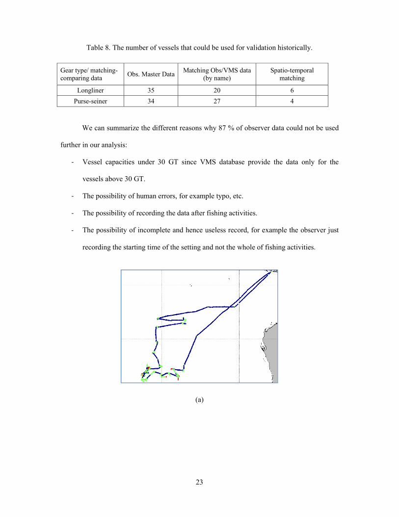
23

Table 8. The number of vessels that could be used for validation historically.

We can summarize the different reasons why 87 % of observer data could not be used

further in our analysis:

- Vessel capacities under 30 GT since VMS database provide the data only for the

vessels above 30 GT.

- The possibility of human errors, for example typo, etc.

- The possibility of recording the data after fishing activities.

- The possibility of incomplete and hence useless record, for example the observer just

recording the starting time of the setting and not the whole of fishing activities.

(a)

Gear type/ matching-comparing data Obs. Master Data Matching Obs/VMS data

(by name) Spatio-temporal

matching

Longliner 35 20 6 Purse-seiner 34 27 4

24

(b)

(c)

25

(d)

(e)

(e) Fig. 7. Track of fishing vessels that show fishing activities from VMS data (dark blue: non-fishing;

green: fishing) correlated with observer data (red: setting; yellow: hauling), a, b, c, d, e: for longliners.

26

(f)

(g)

(h)

27

(i)

Fig. 8. Track of a fishing vessel that shows fishing activities from VMS data (dark blue: non

fishing; green: fishing) correlated with observer data (red: setting; yellow: hauling), f, g, h, i: for

purse-seiners.

Fig. 9. Example of position mismatch between the VMS track (dark blue: non fishing; green:

fishing) and observer data (red: setting, yellow: hauling) for longliners.

28

This analysis emphasizes two recomendations: the need for improved data acquisition

procedures for at-sea observers and the priority to focus on fishing vessels > 30 GT equipped

with VMS. Verification procedure after recording observer data by the supervisor is strongly

important to validated data entry.

2.8 New Avenue to Use VMS Data: State of the Art

VMS data provided invaluable information more than just for fisheries monitoring and

enforcement purposes. Many potential applications use VMS data to support sustainable

fisheries management and scientific purpose. Many studies have focused to use VMS data to

apply in terms of targeted application such as fishing activities estimation and fishing effort

mapping. For example, Joo et al. [18] used VMS data to infer the behavioral modes of fishing

trips of purse-seine Peruvian fishermen targeting anchovy which were recorded by VMS for

almost 1 record per hour. Fishing, searching and cruising behavioral modes were inferred

using hidden Markov model, hidden semi-Markov, random forests, artificial neural networks

and support vector machines. Hidden semi Markov models were proposed considering that

the fishing activity may be more relevantly characterized through temporal segments and not

on a time-step basis as in hidden Markov model. The discriminative models i.e. RF, ANN and

SVM were choosen as alternative models to be compared because the Markovian models has

a restriction in dealing with several observed variables. The observed variables were speed,

turning angle, changes of speed and turning angle. The quantitative evaluation of these

models was performed using a cross-validation procedure according to the groundtruthed data

recorded by at-sea observers. Hidden semi Markov were shown to be the best model for VMS

trajectory analysis with accuracy rate 80.3% [18]. Walker et al. (2010) applied VMS data of

French purse-seine fleet operating in the Indian Ocean and targeting tropical tuna species:

yellowfin tuna (Thunnus albacares), skipjack (Katsuwonus pelamis), and bigeye tuna

(Thunnus obesus) to estimate fishing activity. The observed variables were speeds and turning

29

angles modeled with beta and wrapped Cauchy distributions respectively. The movement

states (still, tracking, cruising) followed a Markovian process and were inferred in a Bayesian

framework. The observers’ data were used to tune the model parameter, validate the model

and also separation “still” state into fishing activity and stopping. The misdetection rate was

of 10% for fishing and non fishing activities, and the under-detection rate on the fishing sets

was of 3% [19]. Shui-Kai Chang et al. (2014) classified fishing and non fishing activities

using the VMS data at six-hour intervals of Taiwanese large-scale tuna longliners (LTLL)

fishery. The key elements of fishing day were: the time (morning or afternoon) and the speed

(fast or slow) were analyzed by three approaches i.e. the optimal-speed-time-ranges, the

between-days distance, the within-day distance. The sensitivity rate was measured for

prediction fishing days and the specificity rate for prediction non-fishing days. As

performance criterion, this study used the maximization of the sum of the sensitivity and

specificity (SSS) rates. In case of similar SSS values, the class with the lowest value of the

absolute difference of the sensitivity and specificity rates was selected. The speed at 2-5 kn in

time range 14:00–23:00 for at least one appearance in VMS data was recommended as a

fishing day. The simple classification method may be crude but efficient. Eventhough there is

potential different strategies for longliners vessel i.e. differences in operation times and speed

in every country, this approach can be used as a basis of development other approach [20].

Dinmore et al. (2003) took a study area over 3° latitude and 5° longitude in central north sea

of UK which was fished by beam trawlers to assess the removal of fishing activity due to the

closure of fishing area. VMS data was available for each 2 hours and eliminate the speed over

8 knots. The temporary closure led to a small increase in the homogeneity of effort

distribution over year [22]. Murawski et al. (2005) analyses the changes of otter trawlers

fishing effort and as a consequence the seasonal fishery closures in the northeast USA. VMS

data was taken for the vessels with speed 3.5 kn. The impact of seasonal closures attracted

30

more fishing effort after opening than prior to closure although with the same or lower

average catch per effort unit [23]. Mills et al. (2007) estimated trawling effort based on an

analysis of 2-hourly VMS data for UK beam trawlers in the North Sea. Two behavioral modes

(trawling and steaming) were identified by speed and turning angle. The vessels were trawling

at speed 2-8 kn, and steaming for speed > 8 kn. Turning angle of trawling was highly variable

and steaming relatively involved straight lines [25]. Witt and Godley (2007) investigated the

patterns of fisheries activity on annual and seasonal scales by using VMS data from UK-

registered large fishing vessels. Fishing activity was assigned to all fishing trips at speeds

≥3.0 and ≤10.0 km h-1 (~1.5 to 5.5 kn). Fisheries activity was gridded at a spatial resolution of

9 km2 (3 km by 3 km pixel) by summing the number of VMS derived data points coincident

to each pixel over monthly and annual scales. The regions of the UK European continental

shelf (i.e. Western Channel and Celtic Sea, Northern North Sea and the Goban Spur) had

received greater fisheries pressure than the rest of the UK continental shelf fishing zone [26].

Fock (2008) defined principal areas for fisheries at high spatial resolution in German EEZ.

Fishing activity was considered for vessels’ speed smaller than mean fishing speed + 2 kn,

where mean fishing speed < 8 kn (otter and beam trawlers and unspecified trawlers) and < 5

kn (GN, seiners and potters). Principal areas of German EEZ were defined as areas which

75% of the fishing effort was carried out [27]. Harrington et al. (2007) explored fisher catch-

return data and high resolution VMS data to determine the distribution of fishing effort. The

distribution of VMS showed that fishing effort was patchy at 5 x 5 km to 250 x 250 m grid

cell sizes [30]. Lee et al. (2010) developed and tested methods for estimating fishing effort of

UK vessels. VMS data was taken for all type of gear in area from 24°W to 58°E and 47°N to

64°N with estimation of fishing activity at a 3' grid resolution. The proposed method was a

process by removing duplicate VMS records and records close to ports, calculating the time

interval between successive records to identify periods of activity, linking each record to a

31

vessel and gear type, differentiating fishing and non-fishing activity, and summing fishing

records in time and space to estimate fishing effort [32]. Gloaguen et al. (2014) described the

fishing activity by analyzing the trajectories of individual demersal vessels using hidden

Markov hodel with an autoregressive process to the vessel velocity [37]. As a result, the

velocity process parameters were truly affected by the fishing activity. They used data from

the RECOPESCA project which were recorded for shorter time incerements (every 15

minutes) to comply with the autoregressive process.

Some other studies investigated the impact of fishing activities onto the environment

such as seabed damage. For example, Rijnsdorp et al. (1998) analyzed the spatial distribution

of fishing effort by an automated recording system with accuracy about 0.1 nautical mile. The

sample was 25 Dutch beam trawl vessels in 1993-1996. Data were taken from two sources

VIRIS database and APR database (every 6 minutes). Three regimes (fishing, steaming,

floating) were differentiated based on speed of fishing (FS = ± 6 kn as fishing speed centre).

Vessel speed with range FS-2 ≤ S ≤ FS+2 was fishing position; S > FS+2 as steaming

position; and S > FS+2 as floating position. During a four year period, in eight most fishing

rectangles of the North Sea, it was estimated that 5% of the area was trawled less than once in

5 years and 29% less than once in a year. It is showed that 30% of the surface area of the sea

bed was trawled between 1 and 2 times in a year and around 9% was trawled more than five

times in a year [21]. Piet et al. (2007) developed indicators of fishing pressure. The sample

was taken from Dutch beam trawl fleet in the southeastern north sea targeting plaice and sole.

Two databases were used (VIRIS) and APR (6 min) / VMS (2 H). Fishing speed for large

fleets 3-6 kn, and for small fleets 5-8 kn. Pressure indicators were described by four levels :

fleet capacity, fishing effort, frequency trawled, annual fishing mortality [28]. Eastwood et al.

(2007) described an assessment of the spatial extent of human activities on the seabed. For the

32

assessment of fishing pressure, VMS data of beam trawlers, otter trawlers, and dredgers

vessels were used. Fishing speed 1-6 kn for otter trawlers and dredgers, 2-8 kn for beam

trawlers. Demersal trawling affected a minimum of 5.4% to a maximum of 21.4% of the total

seabed [29]. Stelzenmüller et al. (2008) studied the spatio-temporal distribution of fishing

pressure on marine landscape in offshore UK (England and Wales) using VMS data for UK

and foreign fleets of beam and otter trawls, and scallop dredges. Fishing speed was used by

Eastwood et al. (2007) to classify fishing and steaming and the analysis of straight lines as

considered to convert the remaining fishing locations into trawl tracks. Marine landscapes

with coarse or mixed sediments and weak or moderate tide stress were heavily fished [31].

Buhl-Mortensen et al. (2015) explored the impact of otter trawl on substratum and

megabenthos on the shelf (50–400 m) and slope (400–2000 m) in the southern Barents Sea.

VMS data within grid cells 5×5 km was used as a proxy for fishing intensity (FI) in the trawl

marks (TM) analysis and within a 2-km radius around the transects for the megabenthos

records. They used video transects to study the density of trawl marks (TMs) and

megabenthos. The relation of FI to the density of TMs and megabenthos was explored using

linear regression and correspondence analysis. The density of TMs was not directly related to

FI but to bottom type, whereas megabenthos density and diversity had a negative correlation

[34].

A few recent studies explored a method to identify the metier of fishing vessels from

VMS data. For example, Russo et al. (2011) identified the métier of fishing vessels by

examining VMS data with artificial neural networks method. The considered multilayer

perceptron network (MPN) involved an input layer with 33 variables and an output layer with

15 métiers. Using as groundtruthed dataset on-board observations, the trained neural network

yielded a correct classification rate greater than 94% [35].

33

Some other studies attempted to estimate fish abundance. For example, Salthaug and

Johannessen (2006) evaluated the sandeel stock in Norway by taken VMS data every 60

minutes of bottom trawl vessels and landings data. Catch Per Unit Effort (CPUE) was

calculated for the trips during week 16 – 18. During year 2001-2005, total CPUE decreased in

2003-2005 compare to 2001-2002. CPUE of the sandeel with age > 2 years decreased from

2001 onwards. In contrast, CPUE for age 1 year showed an increase in 2005 [24].

References

[1] FAO, “The state of world Fisheries and Aquaculture”, 2016.

[2] Ministry of Marine Affairs and fishieries (MMAF), “Marine And Fisheries in Figures

2015”, The centre for data, statistics, and information-MMAF, 2015.

[3] Decree of the Minister of Marine and Fisheries No. 107/KEPMEN-KP/2015, "Fishery

Management Plan for Tuna, Skipjack Tuna, Eastern little tuna", 2015.

[4] B. Realino et al., “Pola Spasial Dan Temporal Kesuburan Perairan Permukaan Laut di

Indonesia (Spatial and Temporal Patterns of Sea-Surface Waters Fertility in

Indonesia)”, Center for Marine Research and Observation, MMAF, 2006.

[5] Ministry of Marine Affairs and fishieries (MMAF),“Keragaan Perikanan Tangkap 2015

( Performance of Fishing 2015)", 2015.

[6] FAO, “The state of world Fisheries and Aquaculture”, 2014.

[7] Irianto, H. E., et al., “Indonesia National Report to The Scientific Committee of The

Indian Ocean Tuna Commission”, 2015.

[8] FAO,” International Plan of Action to Prevent, Deter and Eliminate Illegal, Unreported

and Unregulated fishing”, Rome, 2001.

[9] Agnew, D. J., et al., “Estimating the Worldwide Extent of Illegal Fishing”, PLoS ONE

34

4(2): e4570. doi:10.1371/ journal.pone. 0004570, 2009.

[10] Sodik, D. M., “Combating illegal, unreported and unregulated fishing in Indonesia

Waters: the need for fisheries legislative reform”, University of Wollongong, 2007.

[11] Sodik, D. M., “Analysis of IUU Fishing in Indonesia and the Indonesian Legal

Framework Reform for Monitoring, Control and Surveillance of Fishing Vessels”, The

International Journal of Marine and Coastal Law24 : 67-100, 2009.

[12] Ministry of Marine Affairs and Fisheries, “Statistics of PSDKP”, 2015.

[13] Ministry Decree No.KEP.50/MEN/2012, " National Plan of Action for Preventing and

deterring IUU Fishing in 2012-2016", 2012.

[14] Ministry of Marine Affairs and Fisheries, “ Principal Data Analysis of Marine and

Fisheries”, 2015.

[15] FAO, “Second Global Fisheries Enforcement Training Workshop”, Fisheries and

Aquaculture Report No. 885, 2008.

[16] D.A Varkey et al., “Illegal, Unreported and Unregulated Fisheries Catch in Raja Ampat

Regency, Eastern Indonesia”, Marine Policy 34 : 228-236, 2010.

[17] G.A Wagey et al., “A Study of Illegal, Unreported and Unregulated (IUU) Fishing in

the Arafura Sea, Indonesia”, Research Centre for Capture Fisheries, Agency for Marine

& Fisheries Research, Ministry of Marine Affairs and Fisheries, 2009.

[18] Joo, R., S. Bertrand, J. Tam, R. Fablet,, "Hidden Markov Models: The Best Models for

Forager Movements?", PLoS ONE 8(8):e71246. doi : 10.1371/journal.pone. 0071246,

2013.

[19] Emily Walker, Daniel Gaertner, Philippe Gaspar, Nicolas Bez, “Fishing Activity Of

Tuna Purse Seiners Estimated From VMS Data And Validated By Observers’ Data”,

2010.

[20] Chang, S. K., Tzu-Lun Yuan, “Deriving high-resolution spatiotemporal fishing effort of

35

large-scale longline fishery from vessel monitoring system (VMS) data and validated

by observer data”, Canadian Journal of Fisheries and Aquatic Sciences, 71 (9), 1363-

1370, 2014.

[21] Rijnsdorp, A. D., Buys, A. M., Storbeck, F., and Visser, E. G. “Micro-scale distribution

of beam trawl effort in the southern North Sea between 1993 and 1996 in relation to the

trawling frequency of the sea bed and the impact on benthic organisms”, ICES Journal

of Marine Science, 55: 403– 419, 1998.

[22] Dinmore, T. A., Duplisea, D. E., Rackham, B. D., Maxwell, D. L., and Jennings, S.

“Impact of a large-scale area closure on patterns of fishing disturbance and the

consequences for benthic production”, ICES Journal of Marine Science, 60: 371– 380,

2003.

[23] Steven A. Murawski, Susan E. Wigley, Michael J. Fogarty, Paul J. Rago, and David G.

Mountain, “Effort distribution and catch patterns adjacent to temperate MPAs”, ICES

Journal of Marine Science, 62:1150– 1167, 2005.

[24] Salthaug, A., and Johannessen, T., "The Norwegian in-year monitoring fishery for

sandeel in the North Sea using satellite-based VMS data and landings information",

ICES, 2006.

[25] Mills, C. M., Townsend, S. E., Jennings, S., Eastwood, P. D., and Houghton, C. A.,

"Estimating high resolution trawl fishing effort from satellite-based vessel monitoring

system data", ICES Journal of Marine Science, 64: 248– 255, 2007.

[26] Witt, M. J., and Godley, B. J., "A step towards seascale conservation: using vessel

monitoring systems (VMS) to map fishing activity", PLoS One, 2: e1111, 2007.

[27] Fock, H., "Fisheries in the context of marine spatial planning: defining principal areas

for fisheries in the German EEZ", Marine Policy, 32: 728– 739, 2008.

[28] Piet, G. J., Quirijns, F. J., Robinson, L., and Greenstreet, S. P. R.., "Potential pressure

36

indicators for fishing, and their data requirements", ICES Journal of Marine Science,

64: 110-121, 2007.

[29] Eastwood, P. D., Mills, C. M., Aldridge, J. N., Houghton, C. A., and Rogers, S. I.,

"Human activities in UK offshore waters: an assessment of direct, physical pressure on

the seabed", ICES Journal of Marine Science, 64: 453– 463, 2007.

[30] Harrington, J. J., Semmens, J. M., and Haddon, M., "Spatial distribution of commercial

dredge fishing effort: application to survey design and the spatial management of a

patchily distributed benthic bivalve species", Marine and Freshwater Research, 58:756–

764, 2007.

[31] Stelzenmüller, V., Rogers, S. I., and Mills, C. M., "Spatio-temporal patterns of fishing

pressure on UK marine landscapes, and their implications for spatial planning and

management", ICES Journal of Marine Science, 65: 1081–1091, 2008.

[32] Lee, J., South, A. B., and Jennings, S., "Developing reliable, repeatable, and accessible

methods to provide high-resolution estimates of fishing-effort distributions from vessel

monitoring system (VMS) data", ICES Journal of Marine Science, 67: 1260–1271,

2010.

[33] Navigs. s.a.r.l, "Fishing Vessel Monitoring Systems: Past, Present and Future", The

High Seas Task Force OECD, Paris, 2005.

[34] Buhl-Mortensen L, Ellingsen KE, Buhl-Mortensen P, Skaar KL, Gonzalez-Mirelis G.,

"Trawling disturbance on megabenthos and sediment in the Barents Sea: chronic effects

on density, diversity, and composition", ICES Journal of Marine Science. 73

(Supplement 1): 98-114, 2015.

[35] Russo, T., Parisi, A., Prorgi, M., Boccoli, F., Cignini, I., Tordoni, M., Cataudella, S,

"When behaviour reveals activity: inferring fishing métier from VMS data by artificial

37

neural network," Fisheries Research 111: 53-64, 2011.

[36] Suhendar, M., "Comparison of vessel monitoring system (VMS) between iceland and

indonesia [final project]", Tech. rep., Ministry of Marine Affairs and Fisheries, 2013.

URL http://www.unuftp.is/static/fellows/document/suhendar12prf.pdf.

[37] Gloaguen P., Mahévas S., Rivot E., Woillez M., Guitton J., Vermard Y., and Etienne

M. P., "An autoregressive model to describe fishing vessel movement and activity",

Environmetrics, 26, 17–28, doi: 10.1002/env.2319, 2014.

38

Chapter 3

VMS-based Trajectory Analyses for the Identification of

Longline Vessel Activities

3.1 Introduction

Trajectory data are key data to understand the behavior of fishing vessels and retrieve

fishing vessels activities [1]. Since Vessel Monitoring System (VMS) technology has been

used, many studies have attempted to discriminate fishing vessel activities from VMS data

in order to manage sustainable fisheries [2] for example to estimate fishing effort [3,4,5,6],

to detect illegal vessel gear types [7], mapping fishing area distribution [8], etc. However,

deriving fishing vessel activities from VMS data is still a challenge, especially due to the

differences in VMS data acquisition but also métier-specific variabilities [9].

Many previous studies have been developed to analyze movement patterns of fishing

vessels based on speed and turning angle of VMS trajectories. In general, we could

distinguish three categories of methods to analyze fishing vessel behaviors from their

trajectories, i.e. (i) Simple descriptive statistics, using simple analysis of speed and or

turning angle directly to differentiate fishing vessel activities. (ii) Generative models, using

generative approach for clustering fishing vessels activities. For example, one may cite

GMM, HMM, naive Bayes, (iii) Discriminative models, for example: SVM, RF, neural

networks. These models are considered within a supervised classification framework and

require large groundtruthed dataset. Most of these models have been applied to the analysis

of the VMS trajectories for two fishing gear types i.e. purse-seine [19, 24, 25,], trawl [20,

21], and dredge [22, 23]. In this chapter, we analyze specifically longline fishing vessels,

39

which have not been investigated before using advanced statistical approaches. Simple

classification criterion has been developed to differentiate longline vessel activities based

on speed range and time range [18]. However simple classification feature tend to

overestimate the number of fishing sets [19]. Here, we explored 4 different methods i.e.

simple speed range method as well as HMM, SVM and RF models to infer longline vessel

activities such as steaming, setting and hauling. We aim at determining which method

leads to the best performance for this fishery.

In this study we use VMS data from the Indonesian authorities. Indonesia has been

implementing VMS technology since 2003 in order to monitor the movement of fishing

vessels and also to combat IUU fishing activities for sustainable fishery. VMS device has

been installed onboard more than 4000 fishing vessels including 463 longline fishing

vessels in 2014 (see Fig. 1). The VMS device acquires the Global Position Satellite (GPS)

positions of the fishing vessels and transmitting VMS data almost every hour regularly to

Fisheries Monitoring Centre (FMC) Jakarta by satellite (Argos, inmarsat, iridium, and

Garuda-1).

The purpose of this study is to explore and evaluate different statistical approaches for

the discrimination of the activities of longline vessels derived from VMS data. We

compare the above-mentioned models and consider different inference strategies with a

view to identifying the model that best fits to longliners' VMS data.

40

3.2 Material and Methods

3.2.1 Dataset

In this work, we used two types of data i.e. VMS data and observer data. VMS data

provided by the service in charge of the general surveillance of marine and fisheries

resources (PSDKP-MMAF) Indonesia. Here, we used VMS data specifically for longline

fishing gear type from 2012 to 2014 (see Fig. 2).

Fig. 1. Number of longline vessels installed VMS device in 2012-2014

Fig. 2. Number of VMS data (ping records) from longline vessels that considered as our dataset

400

420

440

460

480

500

520

540

560

2012 2013 2014

Longline

0

50000

100000

150000

200000

250000

300000

350000

Jan Feb Mar Apr May Jun Jul Aug Sep Oct Nov Dec

2012

2013

2014

41

Each ping contained the following information: Vessel ID number, date-time acquisition,

longitude and latitude, speed, heading. Here, we use the speed and turning angle data

derived from VMS trajectory data instead of the features measured by the VMS device.

The VMS device recorded GPS position typically hourly which date and time of VMS data

were recorded in Universal Time Coordinated (UTC) format.

Since 2005, the ministry of marine affairs and fisheries of Indonesia has been

implementing an onboard observer program for monitoring the utilization of fisheries

resources directly and to prevent irresponsible fishing activities. Research Institute for

Tuna Fisheries (LPPT), Benoa-Bali and Directorate of Fisheries Resources (SDI), Jakarta

has been the responsible for collecting observer data. Observers collected the data on the

time and position of fishing activities i.e. setting and hauling activities as well as catch size

and composition. Date and time data were recorded by the observers in local (Indonesia)

time. Overall, we considered more than 450 longline vessels from our VMS dataset and 20

longline vessels from our observers’ data set for vessels between 2012 to 2014.

Here we used observer data for validation purposes by matching VMS data and

observer data. The validation was not trivial due to possibly ambiguous vessel names and

time-position data entry errors. Here we generated an interpolation approach to compare

the shortest distance among vessels in case of mismatch in vessel names. Overall, we only

considered the observer data with a good space-time correlation with VMS data. Overall,

we were left with six observer longline vessels in our study.

42

3.2.2 Instantaneous vs. Calculated Speed and Turning Angle

VMS data sets contain instantaneous speed and heading information provided by VMS

device. Here we compared this instantaneous speed and turning angle information to the

one calculated from the VMS position time series (using haversine formula). The later was

proven more reliable as illustrated in Fig. 3. This might be due to a lesser variability in

terms of rounding (only integer values were recorded e.g., 0, 2, 4, 7 and 17 knots) and also

to missing data in the VMS records of speed and turning angle. This analysis led us to use

speed and turning angle information calculated from consecutive VMS positions.

Fig. 3. The comparison of accuracy rate between vessel speed calculated (VSC) and vessel speed

instantaneous (VSI) using vessel specific model (VSM) based HMM and global model (GM) based HMM.

VSC showed better results for both the VSM model and the GM one. See Section 3.2.3 for details on the

differences between VSM and GM models.

3.2.3 Proposed Approach and Models

Our approach involves two main steps: a preprocessing of the VMS data and the

application of statistical model for the segmentation of a trajectory into activity segments.

0

10

20

30

40

50

60

70

80

90

100

0 0.5 1 1.5 2 2.5

VSC

VSI

GMmodel

VSMmodel

(%)

43

The purpose of the preprocessing step is to remove unreliable, erroneous, or meaningless

VMS data [11]. We proceed as follows: (a) removal of duplicate records, (b) removal of

successive positions less than 5 minutes away, (c) filtering speed outliers, that is to say

VMS positions with a speed whose distance to the mean speed is greater than twice the

standard deviation of the speed over the considered trajectory, (d) removal of VMS

positions close to the port (≤ 3 nautical miles to port), (e) removal of VMS data with a null

speed (0 knot) during more than 24 consecutive hours, what refers to non moving vessels

as transshipment, break engine, docking, ...

As detailed in the following paragraph, we consider four statistical models: a simple

rule-based model, a HMM, a SVM model and a RF model. We evaluate the relevance of

this model using the groundtruthed observer data. Since observer data only recorded two

activities i.e. setting and hauling, we might only consider three component from the model

developed (setting, hauling and others) in order to validate with observer data. We also

explore a segmental approach to improve the accuracy of the segmentation of fishing

vessel activities.

A. Simple rule-based Model

Vessel speed and turning angle are known to be relevant features to differentiate

fishing vessel activities [3, 9]. Higher speed generally relate to steaming state for instance

from and to fishing grounds. By contrast, a slower speed tends to indicate a fishing state.

Overall, longliners' fishing vessel activities can be distinguished into 4 activities i.e.

steaming, i.e. vessel activities from a port to a fishing ground or from a fishing ground to

another fishing ground; setting, i.e. the deployment of baited lines; hauling, i.e. pulling out

hooked lines; waiting, i.e. bait-soaking.

44

Table 1. Speed characteristic to differentiated longliners' fishing vessel activities

State Speed (knot) Fishing Vessel activity 1 > 4 - 6 Setting 2 > 2 - 4 Hauling 3 ≤ 2 ; > 6 Others (e.g.,steaming, soak-time)

Based on the knowledge of speed characteristics of Indonesian longliners as well as

the characteristics of the only two different activities (setting and hauling) recorded by

observer fishery , we may proposed in Table.1 prior tresholding-based rule to be applied to

the hourly speed to help distinguishing three activities i.e. setting, hauling and others.

B. Hidden Markov Model (HMM)

VMS Trajectory analysis with HMM approach has been used widely in fisheries

management (fishing effort mapping, metier identification, etc) due to its performance to

analyze times series data within a well-founded and non-supervised framework [1, 9, 29].

To our knowledge however, the analysis of longliners' trajectory using HMM approach has

not investigated. Here, we proposed a HMM with 4 hidden states, implicitly assuming that

speed and turning angle variabilities are governed by hidden states i.e. state 1 correlated to

steaming, state 2 correlated to setting, state 3 correlated to hauling and state 4 correlated to

soaking time. HMM is a stochastic model with an underlying stochastic process that is not

observable (the sequence of hidden states), but can only be observed through another

process, referred to as the observation sequence. We use a first order (time step between

successive bivelocity is t and t+1) Markov process for the hidden state sequence which is

assumed that the current state only depends on the previous state. Here we used two input

variables i.e. persistent speed (Vp) and turning speed (Vt). Vp and Vt were derived from

speed and turning angle calculated based on time and distance between successive VMS

45

position (see Fig. 4). We calculate correlation coefficients (r) between successive speed

persistent (Vp) and also speed turning (Vt) as shown in Table 2.

Fig. 4. Variables input Vp and Vt

Table 2. Mean correlation coefficient at different time steps between successive speed values (Vp and Vt).

Time step between successive speed

Coefficient correlation (%) ( , ) 79,24 ( , ) 70,96 ( , ) 60,48 ( , ) 55,42 ( , ) 51,23 ( , ) 29,41 ( , ) 9,9 ( , ) 5,42 ( , ) 4,43 ( , ) 3,54

46

The decay of the mean correlation coefficient of the speed features as function of the

time distance supports the assumption of a short-time hidden Markov model. We select a

first-order process in our experiments as a trade-off between model representativity and

model complexity for calibration issues.

For the observation sequence, the observation in time t is independent on previous and

future observations and hidden states conditionally to the hidden state at time t (see Fig. 5)

Figure 5. Graphical state HMM

Formally, the hidden Markov model is defined by the parameter set λ = {A, B, } as

follows:

- A= {aij}, the state transition probability distribution which describes the probability of

a state switches from state Si to Sj between two consecutive time steps.

a = = = ; 1 ≤ , ≤ , is the number of states of the model

0 ≤ a ≤ 1, ∀ , and ∑ a = 1, ∀ .

- B= {bj (Ot)}, the observation probability distribution which describes the probability

of an observation given a state Sj. ( ) = = ; 1 ≤ ≤ , 1 ≤ ≤ , M is the number of distinct

observation symbols per state.

- , the initial state distribution where = ( = )1 ≤ ≤

47

In our study, we consider four hidden states (such as steaming, setting, hauling and

soaking time) and two observed variables, namely Vp (persistent speed) and Vt (turning

speed). For each hidden state, we consider a Gaussian Mixture Model with 3 mixture

components for the observation likelihood for each hidden state, whereas previous works

generally assume a Gaussian distribution. This is regarded as a mean to enrich model

representativity and to better account for intra-state variabilities. The observation

likelihood at time t for state j then resorts to ( ) = = = ∑ ( ; ,Σ ) where are the mixture weights, which define the relative occurrence of the different

modes and satisfy the constraint that ∑ = 1. ; ,Σ is Gaussian

densities with mean μi and covariance ∑i. The number of Gaussian components per state is

here the same for each state in the system.

As in [17], for retrieving the state sequence Q = q1q2...qT given observation

O=o1o2...oT and the model λ, we consider the Maximum Posterior Mode (MPM) sequence

and evaluate posterior likelihoods using a classical Forward-Backward scheme. Variables ( ) = ( = | , ), the probability of being in state Si at time t, given the entire

observation sequence O and the model λ is calculated as follows: ( ) = ( = | , ) = ( ) ( )( | ) = ( ) ( )∑ ( ) ( ) ; ∑ ( ) = 1

where ( ) is forward variable and ( ) is backward variables. Their expressions are

given below. These two variables can be derived analytically from forward and backward

recursions as follows:

48

Forward procedure:

1. Initialization: ( ) = ( )1 ≤ ≤

2. Forward recursion: ( ) = ∑ ( )a ( )1 ≤ ≤ − 1,1 ≤ ≤

3. Termination: ( | ) = ∑ ( )

Backward procedure:

1. Initialization : ( ) = 1 , 1 ≤ ≤

2. Backward recursion: ( ) = ∑ a ( ) ( ), = − 1, − 2, … . . , 1 , 1 ≤ ≤

Overall the MPM inference of the hidden state at time t is given by = [ ( )],1 ≤ ≤

A key feature of the HMM framework is the calibration of all model parameters

λ={A, B, } with respect to a Maximum Likelihood criterion using Baum-Welch method

[17]. We briefly review the main steps of this calibration procedure. Let us define the

probability of being in state Si at time t, and state Sj at time t+1, given the observation

sequence O and the model λ,

( , ) = = , = , = ( )a ( ) ( )( | )

= ( )a ( ) ( )∑ ∑ ( )a ( ) ( ) It may be noted that variable ( ) defined above verifies ( ) = ∑ ( , ). This leads

to the following iterative estimation of the parameters given an evaluation of variables ( , )for current parameter values :

= expected frequency (number of times) in state Si at time (t=1) = ( ) a = expected number of transitions from state tostate

expected number of transitions from state = ∑ ( , )∑ ( )

49

( ) = expected number of times in state j and observation symbol expected number of times in state

= ∑ ( ) .∑ ( )

This iterative procedure is a special case of the general EM procedure applied to HMM. As

initialization, one typically consider uniform priors A and and a randomized

initialization for GMM parameters.

A key challenge in the use of HMM methods the determination of the number of

hidden states. One may consider Bayesian criteria such as AIC and BIC [28]. These criteria

are however prone to overestimation. Here we prefer investigating cross-validation

experiments to evaluate the sensitivity of state identification performance for a

groundtruthed dataset with respect to the number of hidden states in the HMM. Overall, we

considered two different HMM parameterizations:

A HMM model with a Gaussian observation likelihood, that is to say M=1 in [26].

We considered HMM with a number of hidden states from 3 to 20;

A HMM model with a GMM observation likelihood, that is to say M > 1 in [27].

We tested models with M equal to 2 and 3 the number of hidden states varied from

3 to 10.

State identification performance was evaluated in terms of consistence of the hidden states

with respect to the 3 states documented by at-sea observers for longliners, namely setting,

hauling and others.

Regarding model calibration issues, we considered two strategies. We first calibrated a

model gathering the data from all vessels to apply the above-mentioned ML estimation of

HMM parameters. We refer to this model as the global model (GM). The second strategy

relies on the calibration of vessel-adapted models and is referrred to as vessel-specific-

50

model (VSM) strategy. More precisely, for each vessel, we use the global model as an

initialization of the ML procedure for each vessel-specific dataset. As such, we derive

vessel-specific HMM, that is to say that model parameters, including for instance the mean

and covariance of the GMM for each hidden state, which are vessel-adapted. Meanwhile,

based on the common initialization from the global model, we can map the characteristics

of any hidden state for one vessel to the corresponding characteristics for another vessel.

Overall, in the subsequent, we may refer to GHMM-VpVt and GMM-HMM-VpVt as

respectively Gaussian HMM and HMM with a GMM-based observation likelihood, the

terms global vs. vessel-adapted further characterization the considered model calibration

strategy as described in the previous paragraph.

C. Support Vector Machine (SVM)

SVM is a classification method stated as the optimal margin classifier. This classifier

is based on the learning of a separating hyperplane as a linear decision boundary [13]. In

case the separating hyperplane does not exist, it could be solved by using the kernel trick.

It transforms the data into a higher-dimensional feature space, in which a linear decision

boundary can be found [14]. Here, we use radial basis function (RBF) as the kernel

function.

Let us consider a set of training data {( , )} where ∈ ℝ belong to a class ∈ {−1,1}. By SVM, these vectors is mapped into a feature space using kernel function ( , ). The classification function of an SVM is given by:

( ) = ( , ) +

51

where ∈ ℝ and = ( , ,…… . , ) is a vector which maximize the function :

( )ℝ = − 12 ( , ),

subject to

= 0 0 ≤ ≤ = 1,…… . . ,

Parameter C sets a bound on the total number of misclassifications. Increasing the value of

C increases the cost of misclassifying points and decreases generalization power of the

model [1]. The radial basis function (RBF) is defined as follows:

, = − −2

A cross-validation procedure is used to set the kernel and tuning parameters. Here our

feature space is two-dimensional using the two features derived from a VMS trajectory at a

given time step i.e. Vp and Vt. We employed these features to classify three states of

longliners' vessel activities i.e. setting, hauling and others as described above.

D. Random Forest

Random Forest (RF) is another popular classification method. It generates a large

number of trees and then votes for the most popular class [15]. From training data, a

boostrapping procedure is applied to generate decision tress. The data, which are not used

in building a tree, is considered as the “out-of-bag” (OOB) data. These data are used for

estimating the error rate [2]. When generating a tree, a random sample of m variables is

selected as split candidates from the full set of p variables. Take the best variable of m

variables in the top split [16]. Here we apply random forest to the feature vector formed by

Vp and Vt values at a given time step.

52

3.2.4 Performance evaluation

We proceed to the evaluation of the considered models using observers’ data as

groundtruthed data. We first evaluate classification accuracy. It may be noted that the

considered, SVM and RF models are trained in a supervised framework whereas HMM is

trained in a non-supervised framework. To evaluate the classification accuracy to the

hidden states of the HMM, we associated each hidden state to one observers’ state as

follows. For the considered VMS dataset, we first compute the conditional likelihood of

each observers’ state given the inferred HMM state. We then assign to each HMM state the

observers’ state with the greatest conditional likelihood.

In addition to classification accuracy at the hourly time resolution of the VMS

trajectory, we also evaluate whether classification accuracy may according to the duration

of the segments assigned to the same state by the classification methods. As illustrated in

Fig. 6. for a given classification model, we first extract all state segments. For a given time

scale Δ, we can proceed to the computation of mean and state-specific classification

accuracies considering only state segments lasting more than Δ, i.e. withdrawing all

segments with a duration smaller than Δ. We expect this segmental analysis to relate to the

typical duration of each fishing vessel activity.

3.3 Results

3.3.1 Model Performance

We compare the four different methods described above to identify longliners' vessel

activity from VMS trajectory data. To measure the performance of these models, we used a

53

State S1 S1 S1 S1 S1 S1 S2 S2 S2 S2 S2 S2 S3 S1 S1 S3 S3 S3 S3 S3 S1 S1

Time sequences (hours)

1 2 3 4 5 6 7 8 9 10 11 12 13 14 15 16 17 18 19 20 29 30

Segment scale S1 S2 S3 S1 S3 S1 S1

Segment scale with duration >= 3 hours

S1 S2 S3

Fig. 6. Schematic of segment model to consider the characterization behavior of movement ecology hence

might improve the performance of model developed.

cross-validation procedure approach. We may recall that our groundtruthed observer

dataset involved 6 longliners' vessels. We report the mean classification accuracy of the

different models in Table. 3. The HMM method with a four-hidden-state and 3-class

mixture models is shown to outperform the other models (68.5% of mean accuracy vs.

65% for the second best model, see Table 3). Surprisingly, the two supervised

classification models using SVM and RF perform poorly and worse than the simple

thresholding-based classification rules used by SSF model.

Table 3. Classification accuracy of the considered models for the prediction of longliners’ activities from VMS trajectories

No. Model Mean classification accuracy (%)

1 Simple Speed Filter (SSF) 64,9

2 HMM Global Model (GM) 67,9 Vessel Specific Model (VSM) 68,5

3 SVM 57,4 4 RF 57,7

We identified that our dataset may involve some variability. When considering only 3

of the vessels, we resorted to a much greater mean classification accuracy of 79,38% for

the HMM method. The same pattern was observed for the three models. As illustrated in

Fig. 7, 8 and 9, these results suggest a greater consistency of these 3 vessels and a rather

54

low consistency of observers’ data for the 3 other vessels. That may relate to the

consistency of observers’ data acquisition protocols and data quality issues as well as to a

large variability of longliners’ movement patterns.

We further evaluated the relevance of the HMM method for each observers’ state

along with the influence of the duration of the HMM state segment on the relationship

between HMM and observers states. Overall, we retrieved the setting state involved the

greatest confusion (up to 50% of misclassification for the entire dataset). Hauling activities

were retrieved more accurately (classification accuracy of 67% for the entire dataset).

Overall, the thirds observer state depicted the greatest accuracy (80% for the entire

dataset). Again, much greater accuracy rates were reported using only the partial subset

formed by the three vessels depicting a good across-vessel consistency (mean accuracy of

60%, 80% and 90% for setting, hauling and “other” activities). Besides, our results clearly

illustrated the relationship between the duration of inferred HMM segments and the mean

classification accuracy: the greater the duration, the higher the mean accuracy. This

expected pattern is likely to relate to both the typical time scales of setting and hauling

acitivities (a few hours), such that a lower confusion is expected for longer time segment.

3.4 Discussion and Conclusion

This paper addresses the characterization and discrimination of distinguished

longliners' vessel activities from VMS data. We explore how to distinguish longliners'

fishing vessel activities, such as steaming, setting, hauling, waiting activities, with different

methods, namely a simple rule-based method, a generative method and two discriminative

methods. These methods are representative of the approaches investigated in previous

55

work [18] used a rule-based to discriminate fishing vessel activity based solely on VMS-

derived speed. HMM are certainly the most popular models and were investigated in many

Fig. 7. Activity-dependent distributions of vessel speed for 3 of the considered vessels showing a good

consistency across vessels: ((a). vessel A, (b). vessel B, (c) vessel C).

(a)

(b)

(c)

56

(a)

(b)

Setting time (using 24 hour clock - UTC time)

Setting time (using 24 hour clock - UTC time)

Hauling time (using 24 hour clock - UTC time)

Others time (using 24 hour clock - UTC time)

Hauling time (using 24 hour clock - UTC time)

Others time (using 24 hour clock - UTC time)

57

Fig. 8. Activity-dependent daily distributions of each activity for 3 of the considered vessels showing a good

consistency across vessels:(a).vessel A, (b). vessel B, (c) vessel C.

different studies [1, 9]. We also considered two state-of-the-art discriminative methods,

namely SVM and RF as in [1]. The later were trained within a supervised classification

framework, whereas the HMM framework was trained within an unsupervised

framework.

From a methodological point of view, the proposed HMM method involves two main

contributions. On the one hand, we consider GMM distributions for the state-dependent

observation likelihood. Previous works investigated a variety of single-mode parametric

distributions, among others beta and Wrapped Cauchy distributions [12]; generalized

(c)

Setting time (using 24 hour clock - UTC time)

Hauling time (using 24 hour clock - UTC time)

Others time (using 24 hour clock - UTC time)

58

Pareto, generalized extreme value, Laplace and Gumbel distributions [1]. Our choice for

GMM distributions is motivated by the structure of the considered observers’ dataset. We

Speed of vessel D Acquisition time of vessel D

Fig. 9. Activity-dependent distributions of the speed and the time of each vessel activity for 3 of the

considered vessels showing a poor consistency across vessels: (a). vessel D, (b). vessel E, (c) vessel F.

(a)

(b) Speed of vessel E Acquisition time of vessel E

Speed of vessel F Acquisition time of vessel F

(c)

Setting time (using 24 hour clock- UTC time)

59

Table 4. Classification accuracy of the HMM method for the considered segmental analysis at different time-scale for the entire dataset (6 vessels)

Time duration Accuracy rate (%) Data loss (%)

>= 1 70,8 4,9 >= 2 72,4 9,1 >= 3 73,3 13,3 >= 4 74,1 19,7 >= 5 74,7 25,9 >= 6 75,2 33,9

Table 5. Classification accuracy of the HMM method for the considered segmental analysis at different time-scale for the partial dataset (3 vessels with a good across-vessel

consistency)

Time duration Accuracy rate (%) Data loss (%) >= 1 81,8 4,0 >= 2 83 7,5 >= 3 83,5 10,9 >= 4 84,1 16,1 >= 5 84,3 21,5 >= 6 84,5 29,6 >= 7 85,0 36,1

Table 6. Relationships between observers’ states and HMM states for the entire dataset (6 vessels)

P(Obs|Zhmm=k) S1 S2 S3

Setting 0,5 0,1 0,1 Hauling 0,1 0,6 0,1 Others 0,4 0,3 0,8

Table 7. Relationships between observers’ states and HMM states for the entire dataset (3 vessels with a good across-vessel consistency)

P(Obs|Zhmm=k) S1 S2 S3

Setting 0,6 0 0.05 Hauling 0.1 0,8 0,05 Others 0.3 0,2 0,9

Table 8. Relationships between observers’ states and HMM states for the entire dataset (6 vessels) considering only HMM state segment lasting more than 6 hours.

P(Obs|Zhmm=k) S1 S2 S3

Setting 0,5 0,0 0,1 Hauling 0.1 0,7 0,1 Others 0.4 0,3 0,8

60

Table 9. Relationships between observers’ states and HMM states for a partial dataset (3 vessels with a good accross-vessel consistency) considering only HMM state segment lasting more than 6 hours.

P(Obs|Zhmm=k) S1 S2 S3 Setting 0,6 0.1 0.1 Hauling 0.0 0.8 0.0 Others 0.4 0.1 0.9

were provided with two well-defined activity states, namely for setting and hauling

activities. The third state referred to the remaining time periods. As such, it might involve

various activities, such as waiting time between setting and hauling operations as well as

displacement periods between fishing grounds and/or ports. This third state should clearly

involve multimodal speed and heading patterns. It then provided a strong motivation for

GMM-based observation likelihoods, which offer a great modeling flexibility. On the other

hand, we also proposed an original vessel-specific calibration of the HMM. We trained

vessel-specific HMM using as initialization a HMM model trained from the entire VMS

dataset. This training strategy guarantees that (i) the hidden states of the vessel-specific

models can still be matched to reference vessel-independent hidden states, (ii) the trained

models better adapt to vessel-specific patterns. The first property is key to apply the

proposed HMM-based framework calibrated from observers’ datasets to any new VMS

dataset with no observer data, while accounting for inter-vessel variabilities due to vessel

characteristics.

We performed a quantitative evaluation of the performance of three types of models

considered in our study in terms of classification accuracy, i.e. the consistence of the state-

based segmentation of these models with respect to observers’ segmentation in terms of

fishing vessel activities. Overall, in agreement with [1], HMM were clearly the best models

(mean classification accuracy of 82%). Surprisingly, SVM and RF led to poor

classification performance. This might relate to some inconsistency revealed by our

61

analysis in our observers 'dataset for 3 of 6 vessels. For these vessels, the speed and

heading distributions for each activity did not involve any clear pattern in contrast to the

other 3 longliners. This may stress data quality issues in our observer dataset. When

considering only 3 vessels, the mean classification accuracy for the HMM scheme

increased to 13,9%. In our opinion, these experiments emphasize the greatest robustness of

HMM-based schemes compared to supervised discriminative models. As HMM exploits an

unsupervised training strategy, there are less prone to low-quality groundtruthed data. By

contrast, discriminative models are by essence greatly affected by such low-quality

groundtruthed dataset.

These results emphasize the need for higher-quality observer data. Even if HMM were

shown to be more robust, from the original observers’ dataset with 20 longliners, only 3

actually appeared consistent to proceed to a quantitative evaluation. This greatly affects the

potential impact of our study for an operational use. With a mean classification accuracy of

82% (based on: 3 vessels with consistence pattern, vessel-specific models, three season-

specific models, and 6 hours state segments) we consider our results as a promising

evaluation of the potential of HMM-based scheme for the discrimination and identification

of longliners’ activities from VMS data. Complementary analyses even demonstrated that

the classification accuracy could be increased to 4.9 % when considering three season-

specific models, namely June-September (dry season), December-March (wet season) and

April-May & October-November (transition season). We also showed that classification

accuracy increased with the duration of the inferred state segments. The later might be of

particular importance when calibrating fishing effort models and might suggest considering

duration-specific calibrations. `

62

This study emphasized the critical role of groundtruthed observer data. Overall, our

main recommendation for the implementation of the proposed VMS-based monitoring of

the activities of Indonesian longliners is certainly the deployment of a larger-scale at-sea

observer program with well-defined and controlled data acquisition protocols. This appears

to us as a prerequisite to the operational implementation of the investigated HMM-based

strategies and as the only manner to support the well-foundedness of the generalization to

an entire fishery of the patterns extracted from observers’ datasets.

References

[1] Joo, R., S. Bertrand, J. Tam, R. Fablet,, "Hidden Markov Models: The Best

Models for Forager Movements?", PLoS ONE 8(8): e71246, 2013.

[2] Chang, S. K., "Application of a Vessel Monitoring System to Advance

Sustainable Fisheries Management—Benefits Received in Taiwan", Marine

Policy Volume 35, Issue 2, Pages 116–121, 2011.

[3] Mills, C. M., et al., " Estimating high resolution trawl fishing effort from

satellite-based vessel monitoring system data", ICES Journal of Marine Science,

64: 248–255, UK, 2007.

[4] Walker. E., et al, "Fishing Activity of Tuna Purse Seiners Estimated from VMS

Data and Validated by Observers' Data", SCRS/2009/139 Collect. Vol. Sci.

Pap. ICCAT, 65(6): 2376-2391, 2010.

[5] Gerritsen, H., and C. Lordan, "Integrating Vessel Monitoring Systems (VMS)

Data with Daily Catch Data from Logbooks to Explore The Spatial Distribution

of Catch And Effort at High Resolution", ICES Journal of Marine Science,

68(1), 245–252. doi:10.1093/icesjms/fsq137, Ireland , 2011.

63

[6] Walker, E., and N. Bez, “A Pioneer Validation of a State-Space Model of

Vessel Trajectories (VMS) with Observers Data,” vol. 221 (17), pp. 2008 –

2017, 2010.

[7] Marzuki, M. I., Gaspar, P.,Garello, R., Kerbaol, V., Fablet, R., "Fishing gear

recognition from VMS data to identify illegal fishing activities in Indonesia," in

OCEANS 2015 - Genova, doi: 10.1109/OCEANS-Genova.2015.7271551, 2015.

[8] Natale, F., et al., "Mapping Fishing Effort through AIS Data", PLoS ONE 10(6):

e0130746. doi:10.1371/journal.pone.0130746, 2015.

[9] Vermard, Y., et al., "Identifying fishing trip behavior and estimating fishing

effort from VMS data using Bayesian Hidden Markov Models", Ecological

Modeling, Elsevier, Volume 221, Issue 15, Pages 1757-1769, 2010.

[10] Bishop, C. M., and Lasserre, J., Generative or Discriminative? getting the best

of both worlds. In Bayesian Statistics 8, Bernardo, J. M. et al. (Eds), Oxford

University Press. 3–23, 2007.

[11] Russo, T., D’Andrea, L., Parisi, A., and Cataudella, S., "VMSbase: An R-

package for VMS and logbook data management and analysis in fisheries

ecology". PLoS ONE, 9: e100195. doi:10.1371/journal.pone.0100195, 2014.

[12] Walker, E., et al., ”From forager tracks to prey distributions: an application to

tuna vessel monitoring systems (VMS)", Ecological Applications, Ecological

Society of America, 2015, 25 (3), pp.826-833, 2015.

[13] Trevor Hastie, Robert Tibshirani, Jerome Friedman “The elements of Statistical

Learning”, 2009.

[14] Schölkopf, B. and Smola, A., "Learning with Kernels", MIT Press, Cambridge,

MA., 2002.

[15] L. Breiman, "Random forests", Machine Learning 45 (2001) 5–32, 2001.

64

[16] Trevor Hastie, Robert Tibshirani, Jerome Friedman “The elements of Statistical

Learning”, 2009.

[17] Rabiner, L. R., "A tutorial on hidden Markov models and selected applications

in speech recognition", Proceedings of the IEEE 77:257–286, 1989.

[18] Chang, S. K., Tzu-Lun Yuan, “Deriving high-resolution spatiotemporal fishing

effort of large-scale longline fishery from vessel monitoring system (VMS) data

and validated by observer data”, Canadian Journal of Fisheries and Aquatic

Sciences, 71 (9), 1363-1370, 2014.

[19] S. Bertrand, E. Diaz and M. Lengaigne: Patterns in the spatial distribution of

Peruvian anchovy (Engraulis ringens) revealed by spatial explicit fishing data.

Progress in Oceanography, 79, 379-389, 2008.

[20] Rijnsdorp, A. D., Van Maurik Broekman, P. L., and Visser, E. G., "Competitive

interactions among beam trawlers exploiting local patches of flatfish in the

North Sea", ICES Journal of Marine Science, 57: 894– 902, 2000.

[21] Deng, R., Dichmont, C., Milton, D., Haywood, M., Vance, D., Hall, N., and

Die, D., "Can vessel monitoring system data also be used to study trawling

intensity and population depletion? The example of Australia’s northern prawn

fishery", Canadian Journal of Fisheries and Aquatic Sciences, 62: 611–622,

2005.

[22] Walter, J. F., Hoenig, J. M., and Gedamke, T., "Correcting for effective area

fished in fishery-dependent depletion estimates of abundance and capture

efficiency", ICES Journal of Marine Science, 64: 1760– 1771, 2007.

[23] Harrington, J. J., Semmens, J. M., and Haddon, M., "Spatial distribution of

commercial dredge fishing effort: application to survey design and the spatial

management of a patchily distributed benthic bivalve species", Marine and

65

Freshwater Research, 58: 756– 764, 2007.

[24] Walker. E., et al, "Fishing Activity of Tuna Purse Seiners Estimated from VMS

Data and Validated by Observers' Data", SCRS/2009/139 Collect. Vol. Sci.

Pap. ICCAT, 65(6): 2376-2391, 2010

[25] Joo, R., S. Bertrand, A. Chaigneau, and M. Niquen, “Optimization of an

artificial neural network for identifying fishing set positions from VMS data: An

example from the peruvian anchovy purse seine fishery,” vol. 222 (4), pp.

1048–1059, 2011.

[26] Cappe. O, C. E. Mokbel, D. Jouvet and E. Moulines, "An algorithm for

maximum likelihood estimation of hidden Markov models with unknown state-

tying," in IEEE Transactions on Speech and Audio Processing, vol. 6, no. 1, pp.

61-70, Jan 1998.

[27] Bilmes, J., "A Gentle Tutorial of the EM Algorithm and its Application to

Parameter Estimation for Gaussian Mixture and Hidden Markov Models",

Department of Electrical Engineering and Computer Science; U.C. Berkeley,

1998.

[28] Hamaker, E. L., "Using information criteria to determine the number of regimes

in threshold autoregressive models". Journal of Mathematical Psychology,

53(6), 518–529, 2009.

[29] Peel, D., Good, N.M., "A hidden Markov model approach for determining

vessel activity from vessel monitoring system data", Can. J. Fish. Aquat. Sci.

68, 1252–1264, 2011.

66

Chapter 4

Mapping the Fishing Effort of Indonesian Tuna Longliners

from VMS data

4.1 Introduction

The knowledge of the spatial and temporal distribution of the fishing effort is an

important information for the fisheries management. Previously, logbook data had been

used for estimating fishing effort. These data recorded by the fishers provide information

regarding the vessel data, gear type, fishing locations as well as catch profile [1]. As the

form is filled by the fishers, it may be poorly accurate due to the habit of the fishers [3],

incomplete, for instance fishing location may not be detailed [4]. VMS data appears as a

relevant alternative to the fishing effort since it is an automated recording system. It

generates high quality information and independent of fishers’ declaration [5].

A number of previous studies have investigated such VMS-derived fishing effort

estimations for different fisheries [1, 4, 11, 12]. The general framework relies on the

discrimination of fishing vessel activities from the VMS data. The estimation of the fishing

effort comes to convert the time spent by the fishing vessels into some specific activities

into a fishing effort index. As briefly reviewed in Chapter 3, the discrimination of fishing

vessel activities may rely on simple rule-based schemes using VMS speed data as well as

more advanced statistical analyses, especially generative models such as hidden Markov

model (HMM) [7, 8, 9], and discriminative models such as artificial neural networks

(ANN) [6, 8], random forest (RF) and support vector machine (SVM) [8].

67

The VMS-derived analysis of fishing effort has been investigated for different

fisheries and gear types, including beam trawl [10, 11], purse-seine [6, 7, 8] as well as

dredges, hooks-and-lines, nets, seines, traps, trawls in [4]. Here, we analyze VMS data

collected by the Ministry of Marine Affairs and Fishery (MMAF) and focus on the

Indonesian tuna fishery and more specifically longliners. The estimation of longliners’

fishing effort is a critical issue for the MMAF as Indonesian tuna stocks show a decreasing

trend [16, 19]. Few previous works explored longliners’ fishery. For instance, Chang et al.

proposed simple rule-based methods applied to VMS speed to estimate Taiwanese

longliners’ fishing effort in Pacific Ocean [15]. Such methods are however prone to

overestimation and more advanced statistical analyses [6] might significantly reduce the

uncertainty in fishing effort estimation.

Based on our work dedicated to the characterization and discrimination of longliners’

activities from VMS data (Chapter 3), this study further explores the exploitation of the

proposed statistical methods for the spatio-temporal mapping of longliners’ fishing effort

for the Indonesian tuna fishery. We combine the models introduced in Chapter 3 to spatio-

temporal interpolation tools to evaluate fishing effort maps. In the framework of INDESO

project, we analyze the resulting fishing effort maps with respect to the numerical outputs

of SEAPODYM, an ecosystem dynamical model. This chapter is organized as follows. The

first section briefly describes the importance of the monitoring of the fishing effort to

manage sustainable fisheries. It also discusses several methods that have been explored to

estimate fishing effort using VMS data. The second section explains the model to estimate

fishing vessels activities using VMS data and validated with observer data. In section 3 we

report the mapping of fishing effort distribution as well as a comparison with fishing

68

ground prediction generated by SEAPODYM model. Finally this chapter closed in section

4 with discussion and summary of the major conclusion.

4.2 Materials and methods

4.2.1 VMS data and observer data

VMS technology has been used widely in the world after the issue of the decrease of

fish stock in Portugal in the late 80's [17]. The main purpose of a VMS system is to

monitor the activities of fishing vessels. Indonesia as one of the country with the highest

fishing production has been applied VMS system since 2003 to support sustainable

fisheries. VMS have been installed onboard more than 4000 fishing vessels, making

Indonesia the largest user of VMS worldwide. Vessels with capacity > 30 GT equipped

with VMS device transmit their Global Position System (GPS) position about hourly to the

Fisheries Monitoring Center (provided by MMAF) via satellite communication (Inmarsat,

Argos, Iridium). All these data (e.g., vessel ID, transmitter ID, GPS position, heading,

speed, date-time, and gear type) are in the so-called VMS database [18]. Here, we focus

on longliners’ VMS dataset, which comprises 500 fishing vessels and about 5 575 500

VMS positions from 2012 to 2014.

As described in Chapter 3, Indonesian authorities have been implementing since 2005

an at-sea observer program to monitor onboard the utilization of fishery resources and to

prevent irresponsible and illegal fishing activities. Following the preprocessing described

in Chapter 3, we were provided with a groundtruthed observer dataset for 6 vessels

associated with VMS data. Among these 6 vessels, only 3 shown a good consistency

between speed and heading distributions of the labeled activities, namely setting and

hauling operations. A third class of activities, corresponding to the remaining unlabelled

69

time periods, was considered to form a three-class activity dataset. This dataset was used

for calibration purposes.

4.2.2 SEAPODYM model

We collected numerical simulations of Spatial Ecosystem And Populations Dynamics

Model (SEAPODYM) model developed in the framework of INDESO project and adapted

to the Indonesian archipelago. SEAPODYM provided us an operational modeling of tuna

stock dynamics in Indonesia with a 1/12° resolution. SEAPODYM model simulated

spatio-temporal dynamics of age-structured pelagic fish population under the combined

pressure of fisheries and oceanic variability. It predicts fishing efforts and additional

characteristics such as catchability and selectivity of the fishing gear to predict the fishing

grounds [24, 25, 26, 27]. SEAPODYM forcing involves physical and biological variables

provided by the INDESO project.

We use SEAPODYM numerical outputs for tuna biomass as a potential model

prediction for tuna fishing grounds. We compared these numerical outputs to the VMS-

derived estimation of the fishing effort. This analysis was mainly qualitative.

4.2.3 Modeling and inference of longliners’ activities from VMS data

Vessel Monitoring System (VMS) records and transmits approximately hourly

information such as vessel identification, geographical positions, their acquisition time as

well as the instantaneous speed. Motivated by studies on animal movement ecology for the

identification of behavioral activities [20], several methods have been applied to

developed for the inference of fishing vessel activities from VMS trajectory data [1, 5, 7 ].

As briefly reviewed and evaluated in Chapter 3, Hidden Markov Model (HMM) is

70

certainly the most popular framework. Here, we applied a HMM for the identification of

longliners’ activities, more precisely two classes accounting for setting and hauling

operations and a third class for other activities such as soaking time and traveling from and

to fishing grounds.

VMS data for each point of the trajectory are considered as the observed variables and

the sequence of activities is regarded as a sequence of hidden states which will be inferred

by HMM. Let us denote by the hidden state or activity at time t. We consider a first-

order Markov process such that given the entire state sequence from time 0 to time t-1,

the current state at time t, only depends on the predecessor state . This Markovian

prior leads to the parameterization of the transition matrix which states the likelihood of a

given state at time t given the previous state at time t-1. The HMM also involves an

observation likelihood, which evaluates the likelihood of an observation conditionally

to the associated hidden state . In the considered HMM setting, observation is

conditionally independent on previous and future states and observations given that is

known. Here, observation is a two-dimensional vector using the persistent Vp and

turning Vt speed derived from the VMS positions [13].

Vp = V·cos (θ)

Vt = V·sin (θ)

where V is speed and θ is turning angle. We let the reader refer to Chapter 3 for a more

detailed description of the considered HMM framework. Importantly, the observation

likelihood Pr( | ) involves a Gaussian Mixture Model (GMM) to account for

multimodal state-dependent distributions.

71

In our context, the key properties of the HMM is two-fold: (i) given a trained HMM

model, for any VMS trajectory, we can evaluate the posterior likelihoods Pr( | : ) at

any time t, that is to say the likelihood of being in a given hidden state at time t given the

entire observation sequence : , (ii) all HMM parameters, i.e. transition matrix [Pr( = | = )]and state-dependent GMM parameters, can be calibrated in a non-

supervised way from the analysis of a given VMS dataset using an EM procedure. Here,

we benefit from the later property to account for inter-vessel variabilities of the hidden

states as follows. We first train a global model combining all VMS data from all

longliners. This global model provides a first and coarse characterization of the hidden

state through the associated state-dependent GMM parameters. Using this model as an

initialization for the EM-based calibration of HMM parameters for a vessel-specific

dataset, we resort to a vessel-specific HMM parameterization, whose hidden states can still

be mapped to the hidden states of the global model. Applying this strategy to all vessels,

we are provided with vessel-specific HMM parameterizations with a joint global

interpretation of the inferred hidden states. As described in the next section, this is of key

interest for the VMS-derived estimation of longliners’ fishing effort using observers’ data

to map HMM states to fishing vessel activities.

4.2.4 Estimating longliners’ fishing effort from VMS data

The main objective of this paper is to map the fishing effort of longline fishing vessels

in Indonesia. Following [7, 8, 9], the fishing effort for a given spatial region and time

period is stated as function of the total time spent in different fishing vessel activities.

Given that the considered observer data only involve the identification of setting and

hauling operations but do not provide any means to discriminate other potentially relevant

activities in relation to fishing operations (e.g., waiting time between setting and hauling

72

operations), we define the fishing effort as the total time spent in setting and hauling

activities by the longline vessel fleets. Using observers’ data, this definition resorts to the

evaluation of the transition from HMM states to setting and hauling states: ( ℎ ( )| ) = ( ( )| ( ) = ) ∗ ( ( ) = )| ) where Z is the state of HMM (in this case there are 3 state i.e. setting, hauling and others),

obs is observer data corresponding to the record of time and position when setting and

hauling, k denotes the component of HMM and t is time series.

For a region 90 E-142 E; 6 N-20 S and a time period [t0, t1] given the HMM-based

characterization of VMS data, we evaluate the fishing effort as a sum over all vessels and

exploit the above marginalization with respect to the hidden states of the HMM:

=∑ ∆ ( )∑ ( ( )| ( ) = ) ∗ ( ( ) = )| )..................... (1)

where FE represents the fishing effort derived from VMS data, Obs is observer data

corresponding to the record of time and position when setting and hauling, t is time series, ∆ is a period between successive time (in this case one hour in average), Z denotes the

state of HMM, and k indicates the component of HMM.

Given the calibrated vessel-specific HMM, we can directly evaluate all posterior

likelihoods ( | : ). Hence, the evaluation of the fishing effort requires the calibration

of the conditional likelihoods Pr( | ) where At refers to the fishing vessel activity at

time t. Using observers’ data and inferred hidden states, we can calibrate these conditional

likelihoods for the subset of vessels associated with observer data and apply then to the

entire dataset.

73

Here, we consider a 1/12° grid for the estimation of the fishing effort at each grid point

for a given time period, from one week to a quarter. Given the space-time sampling pattern

exhibited by VMS trajectories, the above estimation of the fishing effort may resort to a

scarcely-resolved and noisy mapping with possibly large missing data areas. As a post

processing, we apply an iterative Laplacian diffusion to smooth out fishing effort maps

[22]. This Laplacian diffusion is equivalent to Gaussian smoothing with a ~1/12° spatial

correlation length. The iterated Laplacian diffusion permits to account for the land pixels in

the considered case-study region.

With a view to evaluating the relevance of the estimated fishing effort mapping, we

compare the resulting fishing effort mappings to SEAPODYM numerical predictions for

tuna density for both big eye tuna (BET) and yellow fin tuna (YFT) species. Besides a

visual analysis, we also evaluate correlation coefficients.

4.3 Results

4.3.1 Mapping fishing effort in bimonthly (2012-2014)

We first report the estimated longliners’ fishing effort maps for two-month periods

using a global HMM model (GM) vs. vessel-specific HMM models (VSM). We depict

both the raw fishing effort maps as well as the interpolated maps associated with a spatial

smoothing based on an iterated Laplacian diffusion. The latter can be regarded as a filtered

version for the raw maps. We focus on two examples, respectively February-March 2012

and June-July 2014 (see Fig. 1, and Fig. 2). The two parameterizations resort to similar

spatial patterns. However It may be noted that the global HMM model lead to more VMS

records labelled as setting and hauling: on average, 6% more than with the vessel-specific

parameterizations (see Fig. 5). Significant differences can also be observed. For instance,

74

the vessel-specific HMM parameterizations seem to enhance some local hotspots, for

instance south-east of Sumatera, south of West Papua (see Fig. 1), west Sumatra and south

of Java (see Fig.2).

We also compared the longline fishing effort of VSM model and SSF model (see Fig.

3). They both involve visually similar spatial patterns. However some differences could be

observed in South of Sumatera, and North of Papua as shown in Fig.3.

In Fig. 4, we compared the distribution of longliner activities between 2 activities

(setting and hauling) and all activities (setting, hauling and others) with grid 1/12° from

February to March 2012. Several differences could be observed significantly in South of

Sumatera, South of Bali and Lombok, North of Papua, and South of Papua as shown in

Fig. 4.

75

Fig. 1. Comparison of longliners’ fishing effort distribution using global and vessel-specific HMM parameterizations in February-March 2012. (a) raw mapping issued from the global parameterization (Eq. 1); (b) smoothed version of the distribution shown in (a) using a Laplacian diffusion; (c) raw mapping issued from vessel-specific parameterizations (Eq 1); (d) smoothed version of the distribution shown in (c) using a Laplacian diffusion. See Section II for details on the different models.

(c)

(a) (b)

(c) (d)

76

Fig. 2. Comparison of longliners’ fishing effort distribution using global and vessel-specific HMM parameterizations in June- July 2014. (a) raw mapping issued from the global parameterization (Eq. 1); (b) smoothed version of the distribution shown in (a) using a Laplacian diffusion; (c) raw mapping issued from vessel-specific parameterizations (Eq. 1); (d) smoothed version of the distribution shown in (c) using a Laplacian diffusion. See Section II for details on the different models.

(a)

(b)

(a) (b)

(c) (d)

77

Fig. 3. The comparison of longliners fishing effort distribution using vessel-specific (VSM) parameterizations (a) and Simple Speed Filter (SSF) parameterization (b) in June- July 2014.

(a)

(b)

78

Fig. 4. The distribution of longliner activities with grid 1/12° from February to March 2012 (a) for only 2 activities i.e. setting, and hauling; (b) for all activities i.e. setting, hauling and others.

(a)

(b)

79

Fig. 5. The aggregate of setting-hauling activities between global HMM model (GM) and vessel-specific HMM model (VSM) generated bimonthly for years 2012-2014.

Hereafter, we select fishing effort prediction from the vessel-specific HMM (VSM) for

two main reasons:

- Vessel-specific HMM parameterizations are expected to better account for the

variabilities of vessel characteristics such as fishing behavior, vessel size, weather

conditions,... For example, it may be expected that the characteristics of large and

modern vessels may differ from the fishing characteristics of smaller traditional

vessels. Fishing activities for good weather conditions and bad ones may also

differ.

- We report a slight improvement of the accuracy rate of VSM model compared with

GM model i.e. 68.5% and 67,89% respectively (see Table. 3 in chapter 3 ).

4.3.2 Mapping of fishing effort in seasonally (2012-2014)

Indonesia weather involves two main seasons i.e. northwest monsoon (NWM) in

December-March (rainy season), southeast monsoon (SEM) in June-September (dry

season). Between these two seasons occur a transitional season i.e. the transition from the

0

50000

100000

150000

200000

250000

GM (2012)

VSM (2012)

GM (2013)

VSM (2013)

GM (2014)

VSM (2014)

Feb-Mar

Apr-May

Jun-Jul

Aug-Sep

Oct-Nov

Dec-Jan

80

rainy season to the dry one (TS-I) in April-May, and the transition from the dry season to

the rainy one (TS-II) in October-November. Fig.6. shows the prediction of the average

fishing effort distribution derived from VMS data for these different seasons in 2012-2014.

In Fig. 6. we might see the highest fishing effort distribution generally occur southwest

Java for almost all season. During the dry season (SEM) and transition season (TS-I and

TS-II) seem larger fishing effort occur in west Kalimantan. Overall there are three regions

of longline fishing grounds i.e. West Sumatera, South Java-and-Bali and North Papua that

seem very regularly occur for all season.

4.3.3 The main hotspot area explored yearly (2012-2014)

Fishing effort maps may be considered to assess the areas that are intensely explored.

This is of key interest for a sustainable management of the fishery. We can easily extract

the zone corresponding to the maximum fishing effort south-east of Sumatra. This hotspot

seems to be remarkably stable among seasons and years, with a clear spatial extent (see

Fig. 7).

Overall, one can notice an increase of the predicted global fishing effort from 2012 to

2014, especially in specific areas, for instance south west of Timor island and North of

West Papua, which depict much larger fishing effort values in 2014 than in 2012 and 2013.

4.3.4. Comparisons of longliners’ fishing effort distributions with SEAPODYM

biomass predictions

We compare in Fig. 8. and Fig. 9. the estimated longliners’ fishing effort to

SEAPODYM prediction for big eye tuna biomass. We consider weekly analyses. Overall,

correlation statistics do not reveal any significant global correlation (see Table 1).

81

Importantly, the south-west-to-north-east gradient exhibited by SEAPODYM prediction,

with a greater biomass predicted in the south-west of the case-study area, is not revealed by

VMS-derived fishing effort maps. Similarly, the later appear patchier than SEAPODYM

predictions. Though a number of local hotspots appear in SEAPODYM predictions but not

in fishing effort estimation and vice-versa, the main hotspot revealed in Fig.5 also exhibits

high-biomass values in SEAPODYM predictions. It may also be noted that some hotspots

of the VMS-derived fishing effort prediction, though not being associated with large

SEAPODYM biomass predictions, are close to local maxima of the SEAPODYM fields.

This relatively low agreement between the VMS-derived and SEAPODYM

predictions may relate both to ecosystem-based modeling hypotheses and the sampling

pattern of VMS data, as discussed in previous works [23].

Table 1. Correlation Coefficient between Tuna Model (BET) and longline-VMS Model

Correlation Coefficient between Tuna Model and VMS Model Date Pearson Kendall

1-7 sept 2014 r 0.0248 tau 0.034 p-value 0 p-value 0

8-15 Sept 2014 r 0.0264 tau 0.035

p-value 0 p-value 0

16-23 Sept 2014 r 0.0204 tau 0.031 p-value 0 p-value 0

24-30 Sept 2014 r 0.017 tau 0.025 p-value 0 p-value 0

82

Fig. 6. Average seasonally VMS-based prediction of longliner fishing effort distribution for years 2012-2014. (a) rainy season (NWM, Dec-Mar); (b) transition season (TS-I, Apr-May and TS-II, Oct-Nov); (c) dry season (SEM, Jun-Sep)

(a)

(b)

(c)

83

Fig. 7. Longline fishing effort distribution for one year period. Red rectangle showed the highest area continually explored each year. (a) 2012; (b) 2013; (c) 2014.

(a)

(b)

(c)

84

VSM Model (1-7 Sep 2014) SEAPODYM Model (1-7 sep 2014)

VSM Model (8-15 Sep 2014) SEAPODYM Model (8-15 sep 2014)

VSM Model (16-23 Sep 2014) SEAPODYM Model (16-23 sep 2014)

VSM Model (24-30 Sep 2014) SEAPODYM Model (24-30 sep 2014)

Fig. 8. Comparison of the VMS-derived longliners’ fishing effort index (left side) and SEAPODYM fishing ground prediction for big eye tuna (BET) (right side) for different weekly periods.

85

VSM Model (1-7 Sep 2014) SEAPODYM Model (1-7 sep 2014)

VSM Model (8-15 Sep 2014) SEAPODYM Model (8-15 sep 2014)

VSM Model (16-23 Sep 2014) SEAPODYM Model (16-23 sep 2014)

VSM Model (24-30 Sep 2014) SEAPODYM Model (24-30 sep 2014)

Fig. 9. Comparison of the VMS-derived longliners’ fishing effort index (left side) and SEAPODYM fishing ground prediction for yellow fin tuna (YFT) (right side) for different weekly periods.

86

4.4 Discussion and Conclusion

This study aimed at mapping the space-time distribution of the fishing effort

associated with Indonesian longliners and analyzing the relationships between VMS-

derived fishing grounds and ecosystem-based model predictions for tuna biomasses.

Following previous works [8, 9, 21], we followed a classical framework based on the

HMM-based segmentation of VMS trajectories into fishing vessel activities and the

mapping of these activities into a spatialized fishing effort index. The later relies on the

exploitation of observers’ data to infer a transition matrix from fishing vessel activities to

fishing effort.

From a methodological point of view, we considered vessel-specific HMM

parameterizations to account for inter-vessel variabilities (e.g., vessel characteristics) as

well as possible space-time variabilities (e.g., weather conditions, season). The adaption of

HMM parameterizations to specific VMS subsets was shown to slightly increase the

agreement between the HMM-based inference and observers’ data. This adaption also

enhanced some local hotspots.

Our experimental results pointed out a low global agreement between tuna biomass

prediction from SEAPODYM model and the spatialized VMS-derived fishing effort.

Previous works (e.g., Joo 2013) also stressed differences between the VMS-derived

mapping of the fishing effort and biomass estimation [23]. For instance, in [23], a limited

spatial consistency was found between VMS-derived fishing effort maps and the

estimation of the spatial distribution of the anchovy of the Peruvian coast. Linking VMS-

derived fishing effort to ecosystem-based model prediction for fish biomasses appear as a

particularly complex objective. On the one hand, we need to better understand the

87

sampling pattern associated with fishing vessels. Fishing vessels might only target large

schools, what might explain the patchier distribution depicted by fishing effort maps.

Indonesian longliners might also remain mainly attached to specific fishing grounds with a

weak exploration of the overall distribution of tuna biomass. On the other hand, the

reported analyses might also point out some limits of SEAPODYM model and of the

underlying hypotheses. A focus to the space-time variabilities of the most significant

VMS-derived hotspots might provide additional means to explore the relation between

tuna biomasses and oceanographic conditions and improve model-based predictions for

mid-term perspective.

Regarding fisheries management, a key interest of the reported VMS-derived mapping

is the picture provided for the space-time variabilities of the fishing effort. As illustrated in

Fig.5 and Fig. 6, we might consider a wide range of time scales from a week to a year. As

such, this mapping might be considered to track in “real-time” the fishing effort for

specific areas of interest over short time periods, and it might support the implementation

of fishing restrictions when the fishing effort exceeds some predefined level. At a yearly

scale, as illustrated in Fig.6, the VMS-derived mapping provides a synoptic view of the

spatialization of the fishing effort and of its temporal evolution. In this respect, the

characterization of the space-time variabilities of the fishing effort in the main fishing

grounds extracted as local high-density regions appear as a relevant direction for future

work with a potential added value for fisheries management issues.

Similarly to Chapter 3 the exploitation of observers’ data is a critical step in the

proposed framework. In the reported preliminary results, we exploited observers’ data

from six different fishing vessels. The representativity of this dataset can obviously be

88

questioned. Besides, our detailed analysis suggested that only three of these six vessels

depicted a poor consistency between the observers’ data and VMS-derived information.

We consider the reported experiments as a preliminary analysis of the potential added-

value of a spatialized VMS-derived fishing effort estimation. In this respect, the illustration

of the potential approach for the identification of fishing hotspots (Fig. 6 and Fig. 7) as

well as the difference between the HMM-based analysis of the VMS data and the raw

VMS dataset are regarded as relevant preliminary results to recommend further

investigation for a future operational use. A key element will be the deployment of a

significant at-sea observer program according to standardized protocols, such that future

VMS-based analyses can rely on representative and high-quality observers’ datasets.

References

[1] Bastardie, F., Nielsen, J.R., Ulrich, C., Egekvist, J., Degel, H., “Detailed

mapping of fishing effort and landings by coupling fishing logbooks with

satellite-recorded vessel geo-location”, Fish. Res. Vol. 106, No.1, p. 41–53,

2010.

[2] Chang, S., K., "Application of a vessel monitoring system to advance

sustainable fisheries management—Benefits received in Taiwan", Marine

Policy Volume 35, Issue 2, p. 116–121, 2011.

[3] Marrs, S.J., Tuck, I.D., Atkinson, R.J.A., Stevenson, T.D.I., and Hall,

C.,“Position data loggers and logbooks as tools in fisheries research: results of a

pilot study and some recommendations”. Fish. Res. 58(1), p. 109-117, 2002.

[4] Lee, J., South, A. B., and Jennings, S., “Developing reliable, repeatable, and

accessible methods to provide high-resolution estimates of fishing-effort

distributions from vessel monitoring system (VMS) data”, ICES Journal of

89

Marine Science, 67: 1260–1271, 2010.

[5] Bertrand, S., Bertrand, A., Guevara-Carrasco, R., Gerlotto, F., “Scale-

invariant movements of fishermen: the same foraging strategy as natural

predators”. Ecol. Appl. 17(2), p. 331–3376, 2007.

[6] Bertrand, S., E. Diaz, and M. Lengaigne, 2008. “Patterns in the spatial

distribution of Peruvian anchovy (Engraulisringens) revealed by spatially

explicit fishing data”, Progress in Oceanography, 79,p. 379-389, 2008.

[7] Walker, E., Daniel Gaertner, Philippe Gaspar, Nicolas Bez, 2010. “Fishing

Activity Of Tuna Purse Seiners Estimated From VMS Data And Validated by

Observers’ Data”, Ecol. Model. 221, p.2008-2017, 2010.

[8] Joo, R., S. Bertrand, J. Tam, R. Fablet,, "Hidden Markov Models: The Best

Models for Forager Movements?", PLoS ONE 8(8):e71246. doi :

10.1371/journal.pone. 0071246, 2013.

[9] Vermarda, Youen, et al, "Identifying fishing trip behavior and estimating

fishing effort from VMS data using Bayesian Hidden Markov Models",

Ecological Modeling, Elsevier, Volume 221, Issue 15, Pages 1757-1769, 2010.

[10] Rijnsdorp, A. D., Buys, A. M., Storbeck, F., and Visser, E. G, 1998, “Micro-

scale distribution of beam trawl effort in the southern North Sea between 1993

and 1996 in relation to the trawling frequency of the sea bed and the impact on

benthic organisms”, ICES Journal of Marine Science, 55: 403– 419, 1998.

[11] Mills, C. M., Townsend, S. E., Jennings, S., Eastwood, P. D., and Houghton, C.

A., “Estimating high resolution trawl fishing effort from satellite-based vessel

monitoring system data”, ICES Journal of Marine Science, 64: 248– 255, 2007.

[12] Russo, T., A. Parisi, M. Prorgi, F. Boccoli, I. Cignini, M. Tordoni, and S.

Cataudella, “When behaviour reveals activity: Assigning fishing effort to

90

métiers based on VMS data using artificial neural networks", Fish. Res. 111,

p.53-64, 2011.

[13] Gurarie, E., et al, "Novel method for identifying behavioral changes in animal

movement data", Ecology Letters,12: 395–408, 2009.

[14] Gloaguen, P. et al., "Is speed through water a better proxy for fishing activities

than speed over ground?"', Aquat. Living Resour. 29 (2) 210, 2016.

[15] Chang, S. K., Tzu-Lun Yuan, “Deriving high-resolution spatiotemporal fishing

effort of large-scale longline fishery from vessel monitoring system (VMS) data

and validated by observer data”, Canadian Journal of Fisheries and Aquatic

Sciences, 71 (9), 1363-1370, 2014.

[16] Irianto, H. E., et al., “Indonesia National Report to The Scientific Committee of

The Indian Ocean Tuna Commission”, 2015.

[17] Navigs. s.a.r.l, "Fishing Vessel Monitoring Systems: Past, Present and Future",

The High Seas Task Force OECD, Paris, 2005.

[18] Suhendar, M., "Comparison of vessel monitoring system (VMS) between

Iceland and Indonesia," Tech. rep., Ministry of Marine Affairs and Fisheries,

2013.

[19] Decree of the Minister of Marine and Fisheries No. 107/KEPMEN-KP/2015,

"Fishery Management Plan for Tuna, Skipjack Tuna, Eastern little tuna", 2015.

[20] Giuggioli, Luca, and Frederic Bartumeus. “FORUM: Animal Movement,

Search Strategies and Behavioural Ecology: a Cross-Disciplinary Way

Forward.” Journal of Animal Ecology, vol. 79, no. 4, pp. 906–909.

www.jstor.org/stable/40835479, 2010.

[21] Peel, D., Good, N.M., "A hidden Markov model approach for determining

vessel activity from vessel monitoring system data", Can. J. Fish. Aquat. Sci.

91

68, 1252–1264, 2011.

[22] Sapiro, G., "Geometric Partial Differential Equations and Image Analysis",

Cambridge University Press, 2001.

[23] Joo, R., "A behavioral ecology of fishermen: hidden stories from trajectory data

in the Northern Humboldt Current System", Doctoral dissertation, 2013.

[24] Bertignac, M. et al., "A spatial population dynamics simulation model of

tropical tunas using a habitat index based on environmental parameters",

Fisheries Oceanography 7, 326–334, 1998

[25] Lehodey, P. et al., "Modeling climate-related variability of tuna populations

from a coupled ocean biogeochemical-populations dynamics model", Fisheries

Oceanography 12 (4), 483 494, 2003.

[26] Lehodey, P. et al., "A spatial ecosystem and populations dynamics model

(SEAPODYM) – Modeling", Progress Oceanography, 2008.

[27] Senina, I. et al., "Parameter estimation for basin-scale ecosystem-linked

population models of large pelagic predators: application to skipjack tuna",

Progress in Oceanography, 2008.

92

Chapter 5

Fishing Gear Identification from VMS-based

Fishing Vessel Trajectories

5.1 Introduction

Overfishing truly threats the sustainability of ecosystem fisheries [1]. Illegal,

unreported, and unregulated (IUU) fishing is regarded as one of the major contribution to

overexploitation of fish stocks and threats to marine ecosystem health [1, 3, 4]. Worldwide,

IUU fishing is estimated to result in losses between $10 billion and $23.5 billion annually

and equal to amount to 11-to-26 million tons [5]. Indonesia is one of the countries with the

highest rate of illegal fishing activities in the world [1].

The utilization of illegal and/or undeclared fishing gear type is among the critical

issues that concern Indonesian authorities. Such IUU activities may relate to the limitation

of the fishing quota for certain gear types (e.g., longliner) as well as the higher profit

expected from certain gear type and gear permit fee issues (e.g., purse seiner). Overall, we

may define two broad categories of gear-related IUU activities: the use of a prohibited

fishing gear (e.g., trawling with two boats, pair seines) and the use of an undeclared fishing

gear (i.e., not matching the official fishing permit). With a view to addressing IUU fishing,

Indonesian authorities have implemented since 2003 a Vessel Monitoring System (VMS)

technology. Initially limited to fishing vessels, which were operating in the Indonesian

regulatory area with a capacity above 60 gross tonnages (GT)1, the VMS monitoring has

been extended to fishing vessels with a capacity above 30 GT since 2013. The VMS

collects Global Positioning System (GPS) positions of the fishing vessels that are

1It may be noted that this was only mandatory for fishing vessels with a capacity above 100 gross tonnages before 2013, but supported

through different governmental programs for 60 GT-to-100 GT vessels.

93

transmitted typically hourly to the Fisheries Monitoring Centre (FMC) by satellite

communication (Argos, Inmarsat, Iridium, and Garuda-1).

VMS data provide invaluable information on the spatial and temporal patterns

depicted by fishing activities at multiple scales [6], which are of operational interest for

fisheries management and fisheries ecology [7]. VMS-related studies mostly focus on the

analysis of fishing vessel activities (e.g., fishing, searching, travelling activities) and on

fishing effort spatialization [8, 9, 10, 11, 12]. Fishing métiers identification has been

developed in [25] to identify the vessel gear types for fisheries where one vessel may be

equipped with more than one fishing gear type. Following [25], we address the recognition

of fishing gears from VMS data with the purpose of designing an operational system for

the identification of unauthorized fishing gear type. We hypothesize that VMS patterns

involve gear-specific features (Fig. 1). We state the recognition of fishing gears as a

classification issue and exploit machine learning techniques [13]. Given a dataset of VMS

trajectories associated with known fishing gears, we investigate different types of features

extracted from VMS trajectories and different classification models. Especially, compared

with [25] we introduce new VMS-derived features based on a non-supervised analysis of

gear-specific VMS datasets. Overall, our system involves three key steps: 1) the definition

of VMS-based discriminative features, 2) the learning of a recognition model from a

supervised training dataset, i.e. a dataset for which we are provided with both the VMS

data and fishing gear information, 3) the application of the recognition model to new VMS

data to check the consistency between the recognized and registered fishing gear. This

paper extends the methods and models introduced in our previous work reported in [14].

94

The subsequent is organized as follows. We describe in Section 5.2 the VMS data used

in this study. The proposed learning-based approach for fishing gear recognition is

described in Section 5.3. We report an experimental evaluation in Section 5.4, and we

further discuss our main contributions in Section 5.5.

5.2 VMS data

In this study, we used VMS data collected in 2012 by the service in charge of the

general surveillance of marine and fisheries resources in Indonesia. Overall, the Indonesian

VMS system collects about 1 200 000 GPS positions monthly from over 3 000 fishing

vessels with tonnage from 60 GT up to over 3 500 GT. These vessels use more than 20

different gear types. Here, we focus on the four main registered gear type categories:

trawlers, longliners, pole-and-liners, and purse-seiners (Fig. 1). In Indonesia, trawls are

mostly used to catch shrimps while the 3 other fishing gears are dominantly used for tuna

fishing.

VMS data used here are first preprocessed to eliminate erroneous and meaningless

data [26]. Preprocessing includes: (i) the removal of duplicate data, (ii) the removal of

positions less than 5 minutes apart from the previous one, (iii) the removal of VMS data

close to ports (up to three nautical miles from ports), (iv) the removal of outliers, as VMS

positions associated with a speed five times greater than the median trajectory speed, and

(v) the removal of long static segments (which generally correspond to vessels in harbor

and, rarely, to vessels stopped at sea). In our dataset, all fishing vessels were registered for

only one gear in the Indonesian central permit database. Gear information was provided by

the Directorate General of Capture Fisheries (DGCF) - MMAF (Ministry of Marine Affairs

and Fisheries of Indonesia).

95

Overall, our dataset involves 1 227 fishing vessels for 5 263 158 VMS positions. From

these positions, we compute the associated speed (V) and turning angle (θ) time series

using first-order finite differences [8]. Hence, each fishing vessel is associated with a

bivariate time series over one year with an approximately hourly resolution. It may be

noticed that the time sampling of VMS positions may not be perfectly regular due possible

transmission issues. In our dataset, more than 70% of our preprocessed VMS dataset

involve time intervals between successive VMS positions of one hour +/- 15 minutes.

Theoretically, this variability in the time sampling may affect the consistency of the

computed speed and turning angle features. Time steps with VMS positions removed from

the analysis in the pre-processing step are flagged as missing data in the processing

described in the subsequent.

5.3 Proposed approach

The proposed approach for fishing gear recognition from VMS data involves four

main steps:

- The preprocessing of VMS data as described in the previous section;

- An unsupervised analysis of VMS-derived turning angle and speed time series;

- The definition of a vector of VMS-based features computed for each fishing

vessel;

- The supervised learning of fishing gear recognition models from the considered

VMS-based feature space.

We detail below the last three steps and the application of the trained fishing gear

recognition models to the detection of abnormal VMS patterns.

96

A. Unsupervised characterization of gear-specific fishing vessel activity from VMS

Trajectories

It is well known that the activities of fishing vessels, e.g. cruising, searching, stopping,

and fishing, can be analyzed from VMS trajectories data [8, 10, 11]. Each activity is

typically characterized by specific patterns in terms of speed and turning angle features.

For instance, whereas cruising involves large speed values and rather low turning angles,

fishing typically relates to low speed but greater turning angle variability. Besides this

general trend, we also expect gear-specific patterns. As an illustration, we depict in Fig. 2

the joint distribution of VMS-derived turning angles and speeds for the four fishing gear

categories considered in this work. It may be noticed that, whereas purse-seine and pole-

and-line categories share common patterns. Longliners clearly depict a different

distribution in relation to the deployment of longlines, which involve different speed and

turning angle characteristics compared to purse-seiners for instance. One can also point out

that these distributions clearly involve mixtures of different modes, which may relate to

different activities, such as cruising, searching, fishing...

Given the above-mentioned observations, we consider gear-specific mixture models to

model the joint distribution of the speed and the turning angle. Such mixture models state

this joint distribution as a weighted sum of elementary modes. Hereafter, a mode of a

mixture model is referred to as a regime as usually termed for fishing activity analysis [10]

and may be interpreted as a fishing activity regime. A key interest of such mixture models

is that one can fit all model parameters from any observation dataset in a non-supervised

way, that is to say without knowing the fishing activity attached to each speed and turning

angle observation. As such, mixture models provide a compact and interpretable

representation of gear-specific movement patterns. In this study, we investigate two

97

different mixture models including the classical Gaussian Mixture Models with a view to

accounting for angular features.

(a) Shrimp trawl

(b) Longline

(c) Pole and line

(d) Purse-seine

Fig.1. Examples of VMS trajectories of Indonesian fisheries for the four fishing gears considered in this study.

98

Gaussian-von Mises Mixture Model (GvMMM)

Formally, a Gaussian Mixture Model (GMM) amounts to the following formulation to

model the joint distribution of speed and turning angle [15]:

( | ) = ( | , ∑ ) where is a 2-dimensional continuous-valued data vector (here speed and turning angle).

wi, i=1,...,N are the mixture weights, which define the relative occurrence of the different

modes. g(x|μi,∑i), i=1,…,M are Gaussian densities with mean μi and covariance ∑i. Each

density is a bivariate Gaussian function of the form,

(a) (b)

(c) (d)

Fig. 2. Joint distribution of VMS-derived turning angles and speeds for the considered gear-specific

Indonesian fisheries: namely,(a) shrimp trawler, (b) longliner, (c) pole-and-liner, (d) purse-seiner.

99

( | , ∑ ) = 1(2 ) / |∑ | / −12 ( − )′∑ ( − )

The mixture weights satisfy the constraint that ∑ = 1. Overall, the parameters of a

GMM are stored in: = { , , ∑ },i= 1,...,M. Here, each component of the mixture,

which is characterized by mean characteristics and associated covariance, may be

interpreted as a specific fishing vessel activity. It may be noted that this GMM assumes

that all the components of vector are real-valued with no specific constraint. As such, it

does not actually deal with the 2π-circularity of turning angle values.

To this end, we investigate two approaches. We first explore the use of circular

statistics, namely von Mises distribution as described in the next paragraph. The second

approach we consider an orthogonal decomposition of velocity [16] as described in the

next section.

With a view to addressing the circularity of turning angle values, one may consider

circular distributions, among which von Mises distribution is one of the most popular [17].

It can be viewed as an extension of the Gaussian distribution of angular-valued variables.

Formally, the von Mises distribution for circular variable θ has the following probability

density function:

( | , ) = ( )2 ( ) ; 0 ≤ < 2 ; 0 ≤ ≤ 2 ; ≥ 0

where C represents the univariate von Mises function, β represents the mean direction, k

denotes a scale parameter to measure the concentration of angle, with limit case k=0

corresponding to a uniform distribution and k=∞ a Dirac delta distribution, and ( ) is the

normalization factor of the distribution given by the modified Bessel function of the first

kind of order 0:

100

( ) = 12 ( ) = 1( !) 2∞

This von Mises distribution can represent, using different values for scale parameter k,

both low directional variabilities as observed for steaming activities as well as higher

variabilities expected for fishing activities. It can also represent specific geometric patterns,

which may involve non-null mean directional shift. For instance, trawl-based fishing

patterns depict significant occurrences of ±π turning angle values, which relate to trawling

events (Fig. 2).

We exploit such unimodal von Mises distribution in a mixture model setting. Under

the assumption that speed and turning angle are statistically independent variables, we

consider the following Gaussian-von Mises mixture model (GvMMM) for the joint

distribution of speed ( ) and turning angle (θ):

( , θ| ) = ( | ,σ )C β ,

For the GvMMM, mixture model parameters λ comprise for each model i the mean speed

and the associated standard deviation σ , g represents the univariate Gaussian function,

the mean direction β and the associated scale parameter as well as the prior . Given

the assumption for statistical independence between speed and turning angle, this mixture

model cannot account for the possible correlation between these two variables for a

particular mode. Copula-based models [31] could account for such intra-mode correlation,

however at the expense of a greater computational cost within a mixture model framework.

101

Gaussian Mixture Model VpVt (GMM-VpVt)

This second approach comes to transform the two-dimensional vector formed by the

speed (V) and the turning angle (θ) to a two-dimensional vector accounting for:

- the persistent velocity, denoted by Vp and defined as the component of the velocity

in the current movement direction, computed as V∙cos (θ) [16]

- the turning velocity, denoted by Vt defined as the component of the velocity

orthogonal to the current movement direction, computed as V∙sin (θ) [16].

It may be noted that we do not lose any information with this transformation. The resulting

two-dimensional vector (Vp, Vt) is a real-valued two-dimensional vector, with no

circularity constraint. We can then apply the classical GMM to model the joint distribution

of vector (Vp, Vt). This model is denoted by GMM-VpVt.

ML estimation of mixture model parameters

Given a set of VMS trajectories, we can fit any of the considered mixture models to

the joint distribution of the speed and the turning angle according to Maximum Likelihood

(ML) criterion. To perform this ML inference of the parameters of the mixture model, we

consider an iterative expectation-maximization (EM) algorithm [18]. For the sake of

simplicity, we detail below the implemented EM procedure for the GMM. Let us denote by { } the considered dataset of speed and turning angle feature vectors, and Zk the latent

variable, which states the component the kth data is associated with. The EM algorithm

iterates two steps:

- The E (Expectation) step which evaluates the posterior likelihood of the latent

variable, that is to say the likelihood that feature vector is associated to model :

, = ( = | , ) = ( | , ∑ )∑ ( | , ∑ )

102

- The M (Maximization) step which updates model parameter λ given the posterior

likelihoods computed during the E-step. It comes to the following weighted ML

estimates:

- priors:

= 1 ,

- means:

= ∑ ,∑ ,

- covariance parameters:

, , = ∑ , , ,∑ , −

where index i refer to mode i of the GMM, k to the kth feature vector of the considered

dataset, and index j and l to the components of feature vector . The EM procedure can be

regarded as a gradient-based maximization. In our experiments, we use as a stopping

criterion a threshold on the difference of parameter updates between two consecutive

iterations. Given estimated model parameters, the posterior (as computed during the E-step

of the EM procedure) provides the classification likelihood of any feature vector to be

assigned to a regime or mode of the mixture model.

In the reported experiments, we fit a mixture model for each gear-specific VMS

dataset with the same number of components (typically, 4) and each of the two mixture

models, namely GvMMM and GMM-VpVt. The selection of the number of components

may classically rely on information criterion such as BIC and AIC (27). However these

criteria are sometimes prone to the overestimation of the number of modes in a mixture

model particularly in the ecological framework [38, 39]. In our numerical experiments,

103

cross-validation experiments were used to evaluate the sensitivity of the gear recognition

performance with respect to the number of components. Empirically, considering 4-

component mixture models led to the best performance.

B. VMS-based feature extraction for fishing gear classification

We exploit different types of VMS-derived features for the considered application

fishing gear recognition. For a given fishing vessel, we first extract five classical features

[37] from the associated time series of VMS positions for 2012, respectively the mean

latitudinal and longitudinal position of the VMS trajectory, the associated standard

deviations and a global sinuosity index [36], along with features derived from the fitted

gear-specific mixture models. Besides, from the proposed GMM-based analysis of VMS

datasets, for any calibrated GMM model, we derive the following features:

- The time spent in each regime, computed as the sum over the entire VMS

trajectory of the posterior likelihoods for each vessel. As detailed, for a given

vessel, a VMS trajectory is a time series of hourly VMS positions over one year.

VMS positions filtered during the preprocessing step are considered as missing

data (not-a-number values). The computation of the time spent in a given GMM

component simply comes to counting the number of time steps with a valid (after

preprocessing data) VMS data assigned to the considered GMM component. For

the considered four-gear dataset and given four-component mixture models, this

amounts to 16 features;

- The mean duration of regime segments along the entire VMS trajectory and the

associated standard deviation. A regime segment is defined as a segment of

consecutive time steps which are assigned to a given regime according the

posterior likelihoods. For more details, for a given VMS trajectory, we extract all

104

segments and compute mean segment duration for each component of the GMM.

It may be noted that a regime segment is by construction to time steps with valid

VMS positions as defined by the preprocessing step (cf. Section 2). For the

considered four-gear dataset and given four-component mixture models, this

amounts to 32 features.

Overall, we synthesize in Table. I the considered 53-dimensional feature vector and

distinguish seven types of features, whose relevance for gear recognition is evaluated

hereafter.

C. Supervised Gear Recognition from VMS Trajectories

In this study we consider a supervised classification framework for fishing gear

recognition from the VMS-derived features defined in the previous section. We evaluate

random forest (RF) and support vector machine (SVM) classifiers, which are among the

most popular and efficient machine learning techniques [19, 20, 21]. RF and SVM

classifiers are preferred to neural nets due to a simpler calibration of their hyperparameters

[21].

RF is an ensemble classifier, which builds randomized decision trees [24]. Regarding

the classification step, for a new object and the associated input feature vector, the input

feature vector goes down to a leaf of each tree in the forest. Each tree then votes for a class

and overall, the majority vote over the forest provides the final classification. Here, a RF is

trained by randomly selecting four-fifth of the training data to train each tree of the forest.

The remaining training data are used to estimate error and variable importance. The later

evaluates the classification gain associated with each individual feature. It then provides a

mean to rank the relative importance of the different features in the classification process.

105

SVMs are margin-based classifier. Linear SVMs retrieve hyperplanes that best

separate the training data according to a maximal margin criterion [23]. Non-linear SVMs

exploit an implicit non-linear mapping defined through a kernel function and proceed

similarly to the linear SVMs to best separate the training data in the mapped space. In this

work, the considered kernel is a radial basis function kernel (Gaussian kernel). SVM

parameters are given by the scale parameter of the kernel and a regularization parameter C.

These parameters are empirically selected according to a cross-validation strategy.

For both SVM and RF, we use a repeated 5-fold cross-validation for the evaluation of

the performance of the classification model. This comes to repeatedly use 80 % of the data

for training and 20% for testing. The resulting recognition performance can be regarded as

a representative evaluation of the performance of a VMS-based recognition of the gear

type from new VMS trajectories.

Based on this supervised learning framework, we consider the following strategy to

detect possible abnormal VMS patterns within a given VMS dataset. Using multiple cross-

validation runs, we evaluate the misclassification rate of each vessel of the dataset when it

belongs to the test dataset. Vessels, which involve misclassification rates above a given

threshold (typically 50%), are considered as vessels possibly depicting an abnormal VMS-

related behavior with respect to the vessels within the same fishing gear category. This

strategy allows us to deal with possibly erroneous training data, which may affect the

learning stage of the recognition model.

106

5.4 Results

A. Gear recognition performance

The confusion matrices of the trained classification models are reported in Tables II &

III for respectively SVM and RF classifiers. Overall, we report mean correct recognition

rates of SVM and RF recognitions models trained for VMS-based features issued from the

different mixture models as follows: GvMMM = 97.5% vs. 95.2% and GMM-VpVt =

97.6% vs. 96.8% using respectively SVM and RF classifiers. It shows that the GMM-VpVt

(SVM) method resorts to the highest accuracy rate i.e. 97.6%. The trawl category involves

the highest correct recognition rate (100%) and the longline one the lowest one (92.8%) for

the SVM model. The same holds for the RF model. The greatest confusion is observed

between longline and purse-seine categories. Overall, these results stress the relevance of

our approach for the automated recognition of fishing gear type from VMS trajectories.

Here we further explored SVM method since the SVM showed the highest rate of

accuracy. The two types of mixture models, namely GvMMM and GMM-VpVt, lead to

very similar mean recognition performance (97.5% vs. 97.6%). For these two mixtures

models, we illustrate in Fig. 4 the regime-based segmentation for a VMS trajectory of a

three months longliner, that is to say that for each position along the track we assign the

regime (i.e., the mode of the mixture model) with the highest posterior likelihood (see

Section 3 for details). Though the global segmentation pattern is similar, differences can be

noticed visually, especially for the initial and final segments from and to the port as shown

in Fig. 4. These differences may relate to the ability of the two mixture models to account

for correlation between turning angle and speed. As a matter of fact, intra-regime

variabilities may be expected to exhibit significant correlations between turning angle and

speed.

107

Table 1. Comparison of different vms-based features: we report mean correct classification rates over the four fishing gears using a SVM classifier. we consider four feature types, feature types I and II being derived for a GMM-VpVt model

Feature type

Number of

features Description

Mean correct classification

rate (%) I 16 Relative time spent in each regime 90.5

II 32 Mean and standard deviation of regime segments 85.6

III 3 Sinuosity index + standard deviation of longitude and latitude (GPS position) 41.6

IV 51 I+II+III 93.3

V 4 Vessel mean speed, turning angle, trip duration, and sinuosity index 83.6

VI 441 two-dimensional histogram of speed and turning angle 84.8

VII 53 IV + mean of longitude and latitude (GPS position) 97.6

This is for instance typically expected for longliners, which depict clear geometrical

patterns during setting activities, which should resort in correlated features. Whereas

GMM-VpVt model can handle such correlations, GvMMM parameterization clearly

assumes a statistical independence between speed and turning angle. The rather marginal

differences in terms of mean correct classification rate between GvMMM and GMM-

VpVt model show ever suggest that these correlation characteristics are not of primary

importance to discriminate fishing gear from the proposed VMS-derived features, derived

as mean statistics over a one-year period.

We further evaluate the relevance of each type of features described in Table 1.

Among the different categories of behavioral features (feature types I, II and III), the most

relevant behavior-related features are clearly the times spent in each regime of the gear-

specific mixture models with a recognition rate above 90%, whereas other feature types

report significantly lower recognition performance (below 86%). Especially, the classical

VMS-derived features (feature type III in Table 1) do not prove for the considered case-

108

study (correct recognition rate below 50%). The combination of all behavioral features

results in a mean recognition rate of 93.3%, whereas the additional use of the mean GPS

position improves the mean recognition rate up to 97.6%. We also evaluate the recognition

performance when considering a global regime-based analysis (that is to say, considering

only one mixture model common to all gear types). It results in a loss of about

30% with respect to the proposed gear-specific analysis (Table 4). In Table 1, we also

compare the proposed analysis to other VMS-derived features considered in [25], namely

the joint distribution of speed and turning angle (two-dimensional histogram) illustrated in

Fig. 2 and classical global features (mean speed and turning angle, trip duration and

sinuosity index).The proposed VMS-based features clearly outperform these two feature

sets. Interestingly, we gain about 8% compared with the joint distribution of speed and

(a) (b)

Fig. 3. Segmentation of the fishing regimes along a VMS trajectory using different mixture models for speed and turning angle variables with time period of three months: (a) using GvMMM , (b) using GMM-VpVt. Visually, GMM-VpVt model showed better segmentation results for the initial and final segments from and to port, as stressed by likely misclassified steaming activities in subfigure (a) highlighted by red circles. See Section III for details on the different models.

109

Fig. 4. Distribution of the misclassification rates of the fishing vessels over the entire dataset for repeated 5-fold cross-validation experiments: from multiple cross-validation experiments, we compute for each fishing vessel the misclassification rate as the percentage of misclassification of a fishing vessel when it belongs to the test dataset. We compute the distribution of these misclassification rates over the entire dataset of 1 227 fishing vessels. We only depict the distribution of the non-null misclassification rates, which comprise 47 fishing vessels (misclassification rate=0 (i.e., never misclassified), misclassification rate=100 (i.e., always misclassified)).

Table 2. Confusion matrices for SVM using GvMMM and GMM-VpVt mixture models

YEAR Confusion matrix (SVM) for GvMMM method Mean correct

classification rate (%) Gear Type Trawl

(%) Longline

(%) Pole-and-line

(%) Purse-seine

(%)

2012

Trawl 99.0 1.0 0 0

97.5 Longline 0.1 92.3 0.6 7.0

Pole-and-line 0 0 100 0 Purse-seine 0 1.2 0.2 98.6

YEAR Confusion matrix (SVM) for GMM-Vp/Vt method Mean correct

classification rate (%) Gear Type Trawl

(%) Longline

(%) Pole-and-line

(%) Purse-seine

(%)

2012

Trawl 100 0 0 0

97.6 Longline 0.7 92.8 0.2 6.3

Pole-and-line 0 0 98.8 1.2 Purse-seine 0 1.3 0 98.7

110

Table 3. Confusion matrices for RF models using GvMMM and GMM-VpVt mixture models

YEAR Confusion matrix (RF) for GvMMM method Mean correct

classification rate (%) Gear Type Trawl

(%) Longline

(%) Pole-and-line

(%) Purse-seine

(%)

2012

Trawl 98.6 1.4 0 0

95.2 Longline 0.1 92.1 0.2 7.6

Pole-and-line 0 0.6 92.5 6.9 Purse-seine 0 2 0.5 97.5

YEAR Confusion matrix (RF) for GMM-VpVt method Mean correct

classification rate (%) Gear Type Trawl

(%) Longline

(%) Pole-and-line

(%) Purse-seine

(%)

2012

Trawl 99.7 0.3 0 0

96.8 Longline 0.1 94.0 0.2 5.7

Pole-and-line 0 0 96.4 3.6 Purse-seine 0 2.5 0.3 97.2

turning angle (84.8% using feature types VI vs. 93.3% using feature types IV, vs. 97.6%

using feature types VII cf. Table 1). This further illustrates the relevance of the proposed

features based on a gear-specific regime-based analysis, which also results in a

significantly lower-dimensional feature space.

B. Detection of abnormal VMS patterns

We report in Fig. 4 the distribution of the misclassification rates for the considered

fishing vessel dataset. Interestingly, the distribution of the misclassification rates involves

a multimodal distribution: 93% of the vessels depict a null misclassification rate, 3% a

misclassification rate between 0 and 50% and about 4% (47 vessels among 1 227) a

misclassification rate greater than 50%. We report in Fig. 5 some VMS trajectories, which

relate to the 4% of strongly misclassified fishing vessels.

We further analyzed these misclassified fishing vessels and distinguished three

categories of misclassification sources:

A first category refers to erroneous gear information in the original VMS database.

We performed a cross-checking based on the vessel names with other vessel

111

registration databases2, namely National Database Sharing System for Fisheries

Management provided by Indonesian Ministry of Marine Affairs and Fisheries

(MMAF). We identified that 4 vessels among the 47 detected ones were registered

for a different gear type than the one reported in the considered VMS database. For

instance, the vessel, whose track is reported in Fig. 5.a, is assigned to the longline

gear type in the VMS database, and registered as a purse-seine in vessel

registration databases. It may be noted that for these four examples our model

predicts the gear type retrieved from the complementary vessel registration

databases;

A second category of detected vessels comprises a variety of abnormal patterns

with respect to the registered gear types, which are visually unlikely to involve

illegal fishing gear type. We report a typical example in Fig. 5.c, which depicts the

VMS track of a longliner. This track does not conform to typical longline VMS

patterns and might reveal a transit between ports, which may relate to vessel

maintenance or reconditioning issues.

A last category is interpreted as being related to potential illegal uses of fishing

gears, which do not match the official fishing permit. This hypothesis is strongly

supported for two vessels registered as pole-and-line fishing vessels in the

Indonesian VMS databases, but suspected to involve longline-like behavior from

our analysis. This analysis is in agreement with their registration as longliners in

the list of the authorized tuna fishing vessels maintained by the regional fisheries

management organization. This may be motivated by the fact that the Indonesian

fishing permit fee is lower for pool-and-line vessels compared to longliners. It

illustrates the needs for additional coordination between national and regional

2Given possible slight differences in the names or in the orthography of these names, this cross-checking was performed manually and

could not be straightforwardly automated.

112

fisheries management bodies, which the proposed automated VMS-based analysis

could assist in.

(a) (b)

\\

(c) (d)

Fig. 5. Examples of VMS trajectories associated with a high misclassification rate (above 50 %): (a) longliner misclassified as a purse-seiner, (b) purse-seiner misclassified as a longliner, (c) shrimp-trawler misclassified as a longliner, and (d) pole-and-line misclassified as a purse seiner.

These results demonstrate the relevance of the proposed learning-based approach to

detect abnormal VMS patterns with respect to the registered gear information provided the

Indonesian Ministry of Marine Affairs and Fisheries. It also illustrates the requirement for

further analysis to distinguish illegal fishing activities from other possible reasons for

abnormal behaviors.

113

Table 4. Classification performance using a gear-independent GMM-based analysis: we report mean correct classification rates over the four fishing gears using a SVM classifier and a single GMM-VpVt model trained from all VMS data rather than gear-specific GMM-VpVt models as in Tables, 1, 2 and 3.

Feature type

Number of features Description Percentage

accuracy rate (%) I 4 Relative time spent in each regime 64.6 II 8 Mean and standard deviation of regime segments 64.5

5.5 Discussion and conclusion

This paper explored learning-based and regime-based methods for fishing gear

recognition from VMS data and their application to detecting abnormal VMS patterns of

fishing vessels in Indonesian fisheries. To the best of our knowledge, this is the first

application of the regime-based analysis of VMS trajectories [8, 9, 10, 11] to fishing gear

recognition. We derived different types of VMS-based features from this unsupervised

analysis and combined these features with state-of-the-art supervised classification models,

namely random forests and SVMs. We performed a comparative evaluation with other VMS-

derived features considered such as speed and turning angle distribution [25], trip duration

[25, 37], and sinuosity index [8, 36]. In our numerical experiments, SVMs, which involve a

lower computational complexity, outperformed random forests. The features derived from

gear-specific mixture models, especially the relative time spent into the identified gear-

specific regimes, were shown to greatly contribute to the quality of the recognition

performance compared to classical VMS-derived features [25] as well as the joint histogram

of speed and turning angle and also a unique global mixture model. Our experiments also

suggest that the proposed VMS-derived features may only be weakly affected by the

irregularity of the time sampling of VMS positions, which is of key interest for operational

applications with possibly different VMS data sources and acquisition characteristics. These

results also stress the relevance of latent class models, such as mixture models and hidden

Markov models, to analyze VMS trajectories [e.g., 10, 11]. Whereas previous works mostly

114

focused on the characterization and discrimination of fishing vessel activities [10, 11], our

work shows that such models also provide a relevant representation of gear-specific VMS

patterns for gear recognition issues. As such, gear-specific VMS patterns may be

distinguished from the existence of gear-specific regimes as well as from differences in the

relative occurrences of the gear-specific regimes over the considered time period. The latter is

regarded as the main source of discrimination for the reported gear recognition performance.

Overall, with the sole use of behavioral features we reached a mean recognition performance

of 93%. The additional use of the mean GPS position of the VMS trajectories led to about

97% of correct gear type recognition. The latter information relates to the mean position of

the fishing zones for the considered gear-type fisheries. Such information is expected to be

discriminative for region-specific fisheries, as most of the Indonesian fisheries. It may

however be less relevant for fisheries with large space-time variability.

We demonstrated here the application of the proposed procedure to VMS trajectories

over a one-year period. We ran additional experiments for one-month and 6-month time

series. We obtained similar recognition performance (about 96.1%), which supports the

genericity of our approach and its applicability to finer time scales. This would for instance

allow monitoring possible changes of the fishing gears for a given vessel from a monthly to a

semesterly scale. It may be noticed that the analysis of different time scales could rely on a

single training of the gear-specific mixture models. Only the SVM or RF classification

models would need to be trained specifically for a given time scale. By contrast, classical

global VMS-based features such as mean sinuosity indices [8, 36] have to be considered with

much care to be computed at a relevant time scale since it showed the lowest accuracy rate

(see Table 1). Our experiments suggest that sinuosity features computed at other time scales,

typically in accordance with the proposed regime-based analysis, might be more relevant. In

115

this respect, the regime-based analysis provides an implicit mean to adapt to the relevant time

scales for the considered fisheries, what might be of key interest for its application to other

fisheries.

From a methodological point of view, we combined unsupervised mixture models and

supervised classification models. Hidden Markov Models (HMMs) [10, 11] may be regarded

as a generalization of the considered mixture models and could account for an additional time

prior. The minor differences observed in terms of gear recognition performance between

GvMMM and GMM-VpVt models (97.5% vs. 97.6%) may however suggest that additional

refinements of the regime-based analysis may not lead to significant improvement in terms of

gear recognition. Future work might rather explore other kinds of VMS-derived features. In

this respect, the link between the proposed features and bag-of-words [28], which are among

the state-of-the-art features for text and image classification issues, supports investigating

Fisher vectors [29]. The success of deep learning frameworks [32] for object recognition and

speech analysis makes also appealing future work exploring the use of deep learning models

with a view to jointly identifying gear-specific features and the associated classification

models.

We presented an original application of the proposed approach to the detection of

abnormal VMS patterns with respect to the registered gear types. We detected abnormal VMS

patterns as repeatedly misclassified vessels within a cross-validation framework. Among the

considered dataset of 1 227 fishing vessels, 47 involved a large misclassification rate above

50%. By definition, no ground truth is available. To check the consistency of these detections,

we performed a cross-analysis based on vessels’ names with other Indonesian and regional

fishing vessel registration databases. We retrieved 6 vessels for which this complementary

116

gear information was consistent with the gear type predicted by our model: four of these

vessels appear to be associated with erroneous gear information in the main Indonesian VMS

registration database, and two vessels are likely to involve false declaration of the gear type to

the Indonesian authorities in relation to fishing permit fees. These results support the

relevance of the proposed framework within the newly operational INDESO system [34, 35]

implemented by the Indonesian Ministry of Marine Affairs and Fisheries to monitor

Indonesian fisheries and combat IUU fishing. While our system can generate alerts based on

the sole use of VMS data, the management of these alerts to trigger gear checks should

involve complementary automatic tools for the cross-analysis of fishing vessel registration

databases. In this respect, the combination of the proposed VMS-based analysis and of

automated text mining tools [30] would permit an automatic update of the gear information in

the VMS registration database as well as an identification of likely illegal behaviors.

Similarly, future work should complement the proposed gear-related analysis with the

detection of other non-fishing VMS patterns (e.g., transit) so that surveillance operators could

focus on the documentation of illicit behaviors. Beyond the Indonesian fisheries, the

genericity of the proposed approach opens new avenues for the VMS-based monitoring of

unauthorized and undeclared fishing gears for other fisheries, typically for time scales from a

few weeks to a year.

References

[1] Petrossian, G. A., "Preventing illegal, unreported and unregulated (IUU) fishing:

A situational approach", Biological Conservation 189, 39-48, 2015.

[2] Worm, B. et al., "Impacts of Biodiversity Loss on Ocean Ecosystem Services",

Science 314, 787, 2006.

117

[3] Polacheck, T., "Assessment of IUU fishing for Southern Bluefin Tuna", Marine

Policy 36 1150–1165, 2012.

[4] Pramod, G., et al., “Estimates of illegal and unreported fish in seafood imports

to the USA”, Marine Policy 48 (2014) 102–113, 2014.

[5] Agnew, D. J., et al., “Estimating the Worldwide Extent of Illegal Fishing”,

PLoSONE 4(2): e4570. doi:10.1371/ journal.pone. 0004570, 2009.

[6] Mills, C. M., et al., " Estimating high resolution trawl fishing effort from

satellite-based vessel monitoring system data", ICES Journal of Marine Science,

64: 248–255, UK, 2007.

[7] Gerritsen, H., and C. Lordan, "Integrating Vessel Monitoring Systems (VMS)

Data with Daily Catch Data from Logbooks to Explore The Spatial Distribution

of Catch And Effort at High Resolution", ICES Journal of Marine Science,

68(1), 245–252. doi:10.1093/icesjms/fsq137, Ireland , 2011.

[8] Walker. E., et al., "Fishing Activity of Tuna Purse Seiners Estimated from VMS

Data and Validated by Observers' Data", SCRS/2009/139 Collect. Vol. Sci.

Pap. ICCAT, 65(6): 2376-2391, 2010.

[9] Ortiz, M., A. J. Rubio, A. Parrilla, "Preliminary Analyses Of The Iccat VMS

Data 2010-2011 to Identify Fishing Trip Behavior and Estimate Fishing Effort",

SCRS/2012/125 Collect. Vol. Sci. Pap. ICCAT, 69(1): 462-481, 2013.

[10] Joo, R., S. Bertrand, J. Tam, R. Fablet,, "Hidden Markov Models: The Best

Models for Forager Movements?", PLoSONE 8(8):e71246. doi:

10.1371/journal.pone. 0071246, 2013.

118

[11] Walker, E., and N. Bez, “A pioneer validation of a state-space model of vessel

trajectories (VMS) with observers data,” vol. 221 (17), pp. 2008 – 2017, 2010.

[12] Joo, R., S. Bertrand, A. Chaigneau, and M. Niquen, “Optimization of an

artificial neural network for identifying fishing set positions from VMS data: An

example from the peruvian anchovy purse seine fishery,” vol. 222 (4), pp. 1048-

1059, 2011.

[13] Battula, B. P., and R. S. Prasad, "An Overview of Recent Machine Learning

Strategies in Data Mining", IJACSA ,Vol. 4, No.3, 2013.

[14] Marzuki, M. I., P. Gaspar, R. Garello, V. Kerbaol, R. Fablet, "Fishing gear

recognition from VMS data to identify illegal fishing activities in Indonesia," in

OCEANS 2015 - Genova, doi: 10.1109/OCEANS-Genova.2015.7271551, 2015.

[15] Bishop, C.M." Pattern Recognition and Machine Learning", Springer, New

York (2006).

[16] Gurarie, E., et al, "Novel method for identifying behavioral changes in animal

movement data", Ecology Letters,12: 395–408, 2009.

[17] Mardia, K. V., et al., “A multivariate Von Mises distribution with applications

to bioinformatics”. The Canadian Journal of Statistics 36.1 : 99–109, 2008.

[18] Paalanen, P., et al., "Feature representation and discrimination based on

Gaussian mixture model probability densities—Practices and algorithms",

Pattern Recognition 39,1346 – 1358, 2006.

[19] Ding, C. H. & Dubchak, I., "Multiclass protein fold recognition using SVM and

neural networks", Bioinformatics 17, 349 –358, 2001.

119

[20] Cutler, D.R., Edwards, T. C, Beard, K.H., Cutler, A., Hess, K.T., et al.,

"Random forests for classification in ecology", Ecology 88: 2783–2792, 2007.

[21] Hastie, T., Tibshirani, R., Friedman, J., "The elements of statistical learning:

data mining, inference and prediction", Springer, 2 edition, 2009.

[22] L. Breiman, "Random forests", Machine Learning 45 (2001) 5–32, 2001.

[23] Schölkopf, B. and Smola, A., "Learning with Kernels", MIT Press, Cambridge,

M. A., 2002.

[24] Maddimsetty, R. P., et al., "Accelerator design for protein sequence HMM

search", In Proceedings of ICS, pages 288–296, 2006.

[25] Russo, T., Parisi, A., Prorgi, M., Boccoli, F., Cignini, I., Tordoni, M.,

Cataudella, S, "When behaviour reveals activity: inferring fishing métier from

VMS data by artificial neural network," Fisheries Research 111: 53-64, 2011.

[26] Russo, T., D’Andrea, L., Parisi, A., and Cataudella, S., "VMSbase: an R-

package for VMS and logbook data management and analysis in fisheries

ecology". PLoSONE, 9: e100195. doi:10.1371/journal. pone. 0100195, 2014.

[27] Hamaker, E. L., "Using information criteria to determine the number of regimes

in threshold autoregressive models". Journal of Mathematical Psychology,

53(6), 518–529, 2009.

[28] Lazebnik, S., Schmid, C.,Ponce, J., "Beyond bags of features: spatial pyramid

matching for recognizing natural scene categories", IEEE Computer Society

Conference on Computer Vision and Pattern Recognition - Volume 2

(CVPR'06) (PDF). 2. p. 2169. doi:10.1109/CVPR.2006.68, 2006.

120

[29] F. Perronnin and C. Dance., "Fisher kernels on visual vocabularies for image

categorization", In Proc. CVPR, 2006.

[30] Zhou, Y., Tong, Y., Gu, R., and Gall, H., "Combining text mining and data

mining for bug report classification", J. Softw. Evol. and Proc., 28: 150–176,

2016.

[31] A. Roy and S. K. Parui, "Pair-copula based mixture models and their application

in clustering", Pattern Recognition, vol. 47. No. 4 pp.1689-1697, 2014.

[32] Yann LeCun, Yoshua Bengio, and Geoffrey Hinton, "Deep learning", Nature

521, 7553 (2015), 436–444, 2015.

[33] Sermanet, P. et al., "Overfeat: integrated recognition, localization and detection

using convolutional networks", In Proc. International Conference on Learning

Representations, 2014.

[34] Tranchant B., Reffray G., Greiner E., Nugroho D., Koch Larrouy Ariane,

Gaspar P. Evaluation of an operational ocean model configuration at 1/12

degrees spatial resolution for the Indonesian seas (NEMO2.3/INDO12) : Part 1:

Ocean physics. Geoscientific Model Development, 9 (3), p. 1037-1064. ISSN

1991-959X, 2016.

[35] Gutknecht, E., Reffray, G., Gehlen, M., Triyulianti, I., Berlianty, D., Gaspar, P.,

"Evaluation of an operational ocean model configuration at 1/12 degrees spatial

resolution for the Indonesian seas (NEMO2.3/INDO12) : Part 2 :

Biogeochemistry", Geoscientific Model Development, 9 , p. 1523-1543, 2016.

[36] Benhamou, S.,"How to reliably estimate the tortuosity of an animal’s path:

121

straightness, sinuosity, or fractal dimension?", Journal of theoretical biology

229:209–20. 10, 2004.

[37] Demšar et al., "Analysis and visualization of movement: an interdisciplinary

review", Movement Ecology, 2015.

[38] Pohle, J. et al., "selecting the number of states in hidden markov model - pitfalls,

practical challenges and pragmatic solutions", arXiv: 1701.08673v1 [stat. ME],

2017.

[39] Biernacki, C., G. Celeux & G. Govaert, "assessing a mixture model for

clustering with the integrated completed likelihood", IEEE Transactions on

Pattern Analysis and Machine Intelligence, 22(7), 719-725, 2000.

122

Chapter 6

Conclusions and Perspectives

VMS has been applied widely in the world to monitor the movement of fishing vessels

and for the enforcement of fishery regulations. After more than a decade, the huge amount of

VMS data collected have strongly supports the exploration of data mining and statistical

frameworks to analyze these VMS data for fisheries management issues, including for

instance fishing gear identification, vessel activity segmentation as well as the evaluation of

fishing effort indices. In the context of INDESO project, the aim of this study is to explore

such methods to support the sustainable managements of Indonesian fisheries, which are

threatened by overfishing and illegal, unreported and unregulated (IUU) fishing activities.

We first reviewed the main characteristics of Indonesian fisheries and stressed the

socio-economic contribution of the fisheries sector in Indonesia (see Chapter 2). Besides, we

described IUU fishing, which threatens the sustainability of the fisheries. We also presented

the at-sea observer program implemented by the Indonesian authorities. At-sea observers’

data are critical groundtruthed data for calibration and validation purposes. Chapters 3 to 5 are

the core of this thesis and investigated statistical analyses of VMS datasets for three

objectives: the discrimination of fishing vessel activities (Chapter 3), the computation of

spatialized fishing effort indices (Chapter 4), and the recognition of fishing gears (Chapter 5).

We reported good correct classification rates (about 70% for longline fishing vessel activity

segmentation and greater than 97% for gear type recognition) and the preliminary analysis of

the VMS-derived fishing effort maps pointed out the added value of the use advanced

statistical analyses compared with the direct use of raw VMS data.

123

From a methodological point of view, we investigated both generative models, namely

Gaussian Mixture Models (GMM) and Hidden Markov Models (HMM), as well as

discriminative models, namely Support Vector Machine (SVM) and Random Forests (RF). In

agreement with (Joo, 2013) [1], our experiments support the greater relevance of HMM for

the analysis of fishing vessel activities. This is regarded as a direct consequence of HMM to

account for time dependencies. The application to gear type recognition provides an example

of a significant combination of generative and discriminative models. We also investigated

more complex HMM with a GMM parameterization of observation models, whereas most

previous works considered simpler unimodal parameterizations. We believe this contribution

suggests future research directions with more complex models. In this respect, the emergence

of deep learning models [2, 3] seems particularly appealing as a means to combine generative

and discriminative models for time-dependent processes. Another important research

direction suggested by our work is the exploration of the “local” adaption of model

parameterizations (locally-adapted vs. global models). Here, the term local may refer to a

specific time periods (e.g. weekly, monthly and yearly), regions (e.g. FMA) as well as vessel

subsets (e.g. vessel size, fishing behavior and weather condition…). Such adaptions are also

referred to as fine-tuning in the machine learning field. Such fine-tuning strategies

investigated here for the segmentation of fishing vessel activities and the mapping of the

fishing effort allowed us to account for inter-vessel as well as time variabilities in vessel

movement characteristics, while maintaining a common interpretation of the identified latent

variables. We believe such fine tuning strategies might greatly contribute to extend the

generalization capabilities of models tuned from relatively small-scale groundtruthed datasets,

which is mostly the case of at-sea observers’ datasets.

124

The reported results support the relevance of the proposed models for a future

operational use. The analysis of observers’ data (Chapter 3) and the application to gear type

recognition (Chapter 5) stress both the high relevance of the datasets collected by Indonesian

authorities and the needs for new tools for an improved data quality. Whereas in Chapter 5

some abnormal behaviors were likely to relate to erroneous gear information in the reference

database, most of the observers’ data could not be used in Chapter 3 as they could be matched

to the VMS dataset (14 vessels could not be used among a total of 20 vessels) and, among the

six vessels linked to observers’ data, three depicted poorly consistent fishing activity features.

These results emphasize the importance of quality check procedures in the acquisition of

fisheries datasets. This should certainly be considered as a priority for the operational

application of the proposed methodology.

Interestingly, as illustrated in Chapter 5, the proposed statistical analyses of VMS data

might also be regarded as new means for the automated evaluation of the quality of the

collected dataset. For instance, the proposed gear type recognition model might be used for

the automated detection of possibly erroneous gear type data in the reference database, for

which further analysis and cross-checking with other data sources might be performed. A

similar procedure could be developed for the automated analysis of at-sea observer data and

could contribute to the regular synchronization of different fisheries-related databases, such as

the VMS and fishing permit databases.

In this thesis, we focused on VMS data. Within the framework of INDESO project, the

Indonesian government has implemented a Radar-based VDS (Vessel Detection System) in

Perancak - Bali as well as the collection of AIS (Automatic Identification System) data as part

of a global MCS (Monitoring, Control and Surveillance) system for Indonesian fisheries,

125

including the detection of IUU fishing. The synergies between these different data sources

appear as particularly appealing and promising for future studies. For example, it is a

challenge for future work to fully exploit the synergy between VMS data and satellite-derived

vessel detection schemes (Radar based VDS) to combat IUU fishing since each satellite image

both radar and optic is very expensive. Model forecast from VMS data could help to predict

critical zone of IUU fishing.

References

[1] Joo, R., S. Bertrand, J. Tam, R. Fablet,, "Hidden Markov Models: The Best

Models for Forager Movements?", PLoS ONE 8(8):e71246. doi:

10.1371/journal.pone. 0071246, 2013.

[2] LeCun, Y., Bengio, Y., Hinton, G., "Deep learning", Nature, vol. 521, no 7553,

p. 436-444, 2015.

[3] Chung, J., et al., "A Recurrent Latent Variable Model for Sequential Data",

Advances in neural information processing systems (pp. 2980-2988), 2015.

�� ������� �� �������

Résumé

Le suivi, le contrôle et la surveillance (MCS) des pêches marines sont

des problèmes essentiels pour la gestion durable des ressources

halieutiques. Dans cette thèse, nous étudions le suivi spatial des

activités des navires de pêche en utilisant les données de trajectoire du

système de surveillance des navires (VMS) dans le cadre du projet

INDESO (2013-2017). Notre objectif général est de développer une

chaîne de traitement des données VMS afin de: i) effectuer un suivi de

l'effort de pêche des flottilles de palangriers indonésiens, ii) détecter les

activités de pêche illégales et évaluer leur importance. L'approche

proposée repose sur des modèles de mélange gaussien (GMM) et les

modèles de Markov cachés (HMM), en vue d'identifier les

comportements élémentaires des navires de pêche, tels que les

voyages, la recherche et les activités de pêche, dans un cadre non

supervisé. Nous considérons différentes paramétrisations de ces

modèles avec une étude particulière des palangriers indonésiens, pour

lesquels nous pouvons bénéficier de données d’observateurs

embarqués afin de procéder à une évaluation quantitative des modèles

proposés et testés.

Nous exploitons ensuite ces modèles statistiques pour deux objectifs

différents: a) la discrimination des différents flottilles de pêche à partir

des trajectoires des navires de pêche et l'application à la détection et à

l'évaluation des activités de pêche illégale, b) l'évaluation d'un effort de

pêche spatialisé à partir des données VMS. Nous obtenons de très

bons taux de reconnaissance (environ 97%) pour la première tâche et

nos expériences soutiennent le potentiel d'une exploration

opérationnelle de l'approche proposée. En raison du nombre limité de

données d’observateurs embarqués, seules des analyses préliminaires

on pu être effectuées pour l’estimation de l'effort de pêche à partir des

données VMS. Au-delà des développements méthodologiques

potentiels, cette thèse met l'accent sur l'importance de la qualité de

données d'observation en mer représentatives pour développer

davantage l'exploitation des données VMS tant pour la recherche que

pour les questions opérationnelles.

Mots-clés : Surveillance spatiale des activités des navires de pêche,

Effort de pêche, Pêche illégale, Données de trajectoire, VMS

l'extraction de données, Apprentissage non supervisé et supervisé

Abstract

Monitoring, control and surveillance (MCS) of marine fisheries are

critical issues for the sustainable management of marine fisheries. In

this thesis we investigate the space-based monitoring of fishing vessel

activities using Vessel Monitoring System (VMS) trajectory data in the

context of INDESO project (2013-2017). Our general objective is to

develop a processing chain of VMS data in order to: i) perform a follow-

up of the fishing effort of the Indonesian longline fleets, ii) detect illegal

fishing activities and assess their importance. The proposed approach

relies on classical latent class models, namely Gaussian Mixture

Models (GMM) and Hidden Markov Models (HMM), with a view to

identifying elementary fishing vessel behaviors, such as travelling,

searching and fishing activities, in a unsupervised framework.

Following state-of-the-art approaches, we consider different

parameterizations of these models with a specific focus on Indonesian

longliners, for which we can benefit from at-sea observers’ data to

proceed to a quantitative evaluation.

We then exploit these statistical models for two different objectives: a)

the discrimination of different fishing fleets from fishing vessel

trajectories and the application to the detection and assessment of

illegal fishing activities, b) the assessment of a spatialized fishing effort

from VMS data. We report good recognition rate (about 97%) for the

former task and our experiments support the potential for an

operational exploration of the proposed approach. Due to limited at-sea

observers’ data, only preliminary analyses could be carried out for the

proposed VMS-derived fishing effort. Beyond potential methodological

developments, this thesis emphasizes the importance of high-quality

and representative at-sea observer data for further developing the

exploitation of VMS data both for research and operational issues.

Keywords : Space-based monitoring of fishing vessel activities,

Fishing effort, Illegal fishing, VMS trajectory data, Data mining,

Unsupervised and supervised learning