Vladimir MatveevJena (Germany)

Integrable systems and geodesicallyequivalent metrics

www.minet.uni-jena.de/∼matveev/

Video of a similar talk is athttp://www.msri.org/calendar/workshops/WorkshopInfo/

446/show workshop

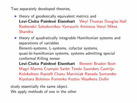
Two separately developed theories,

◮ theory of geodesically equivalent metrics andLevi-Civita Painleve Eisenhart Weyl Thomas Douglas HallRashevskii Solodovnikov Yamauchi Aminova Venzi MikesShandra

◮ theory of quadratically integrable Hamiltonian systems andseparations of variablesBenenti-systems, L-systems, cofactor systems,quasi-bi-hamiltonian systems, systems admitting specialconformal Killing tensorLevi-Civita Painleve Eisenhart Benenti Braden IbortMagri Marmo Crampin Sarlet Tondo Saunders CantrijnKolokoltsov Rastelli Chanu Marciniak Ranada SantanderKiyohara Bolsinov Fomenko Kozlov Waalkens Dullin

study essentially the same object.We apply methods of one in the other

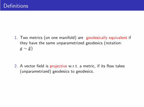
Definitions

1. Two metrics (on one manifold) are geodesically equivalent ifthey have the same unparametrized geodesics (notation:g ∼ g)

2. A vector field is projective w.r.t. a metric, if its flow takes(unparametrized) geodesics to geodesics.

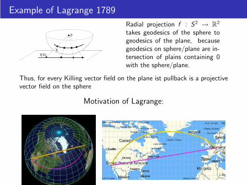
Example of Lagrange 1789

����

����

���

���

����

��������

����

��������

������

������

�������������������������������������������������������������������������������������������������������������������������������������������������������������������������������������������������������������������������������������������������������������

�������������������������������������������������������������������������������������������������������������������������������������������������������������������������������������������������������������������������������������������������������������

���

�������

����

��������

0

f(X)X

Radial projection f : S2 → R2

takes geodesics of the sphere togeodesics of the plane, becausegeodesics on sphere/plane are in-tersection of plains containing 0with the sphere/plane.

Thus, for every Killing vector field on the plane ist pullback is a projectivevector field on the sphere

Motivation of Lagrange:

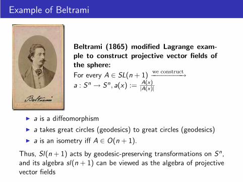
Example of Beltrami

Beltrami (1865) modified Lagrange exam-ple to construct projective vector fields ofthe sphere:

For every A ∈ SL(n + 1)we construct−−−−−−−−→

a : Sn → Sn, a(x) := A(x)|A(x)|

◮ a is a diffeomorphism

◮ a takes great circles (geodesics) to great circles (geodesics)

◮ a is an isometry iff A ∈ O(n + 1).

Thus, Sl(n + 1) acts by geodesic-preserving transformations on Sn,and its algebra sl(n + 1) can be viewed as the algebra of projectivevector fields

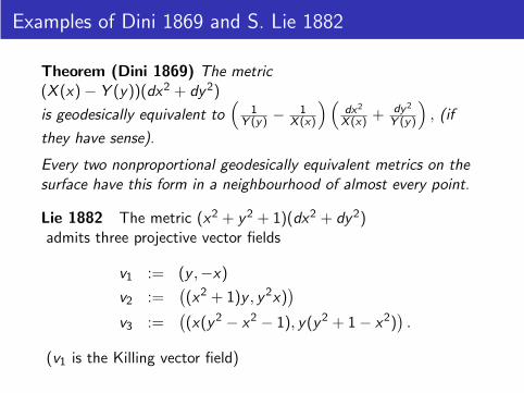
Examples of Dini 1869 and S. Lie 1882

Theorem (Dini 1869) The metric(X (x) − Y (y))(dx2 + dy2)

is geodesically equivalent to(

1Y (y) −

1X (x)

) (dx2

X (x) + dy2

Y (y)

)

, (if

they have sense).

Every two nonproportional geodesically equivalent metrics on thesurface have this form in a neighbourhood of almost every point.

Lie 1882 The metric (x2 + y2 + 1)(dx2 + dy2)admits three projective vector fields

v1 := (y ,−x)

v2 :=((x2 + 1)y , y2x)

)

v3 :=((x(y2 − x2 − 1), y(y2 + 1 − x2)

).

(v1 is the Killing vector field)

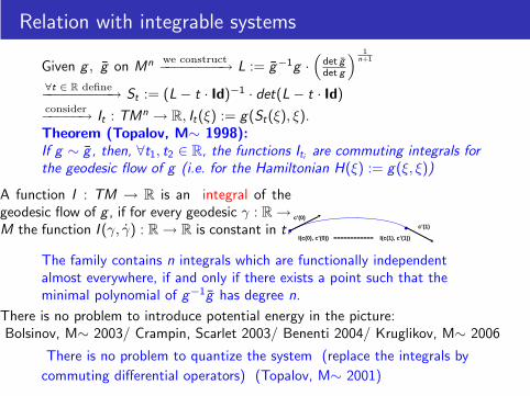
Relation with integrable systems

Given g , g on Mn we construct−−−−−−−−→ L := g−1g ·(

det gdet g

) 1n+1

∀t ∈ R define−−−−−−−−−→ St := (L − t · Id)−1 · det(L − t · Id)consider−−−−−→ It : TMn → R, It(ξ) := g(St(ξ), ξ).Theorem (Topalov, M∼ 1998):If g ∼ g , then, ∀t1, t2 ∈ R, the functions Iti are commuting integrals forthe geodesic flow of g (i.e. for the Hamiltonian H(ξ) := g(ξ, ξ))

A function I : TM → R is an integral of thegeodesic flow of g , if for every geodesic γ : R →M the function I (γ, γ) : R → R is constant in t.

I(c(0), c’(0)) ============ I(c(1), c’(1))

c’(0)

c’(1)

The family contains n integrals which are functionally independentalmost everywhere, if and only if there exists a point such that theminimal polynomial of g−1g has degree n.

There is no problem to introduce potential energy in the picture:Bolsinov, M∼ 2003/ Crampin, Scarlet 2003/ Benenti 2004/ Kruglikov, M∼ 2006

There is no problem to quantize the system (replace the integrals by

commuting differential operators) (Topalov, M∼ 2001)

Plan:

◮ Geometric sense of the integrals

◮ One application of geodesic equivalence to integrable systems:Sinjukov-Topalov hierarchy as a way of constructing integrablesystems

◮ One application of integrable systems to geodesic equivalence:What closed manifolds admit geodesically equivalent Riemannianmetrics?

◮ Combining methods from integrable systems and differentialgeometry: solution of Lie Problem and of Lichnerowicz-Obataconjecture

◮ Geodesic equivalence in general relativity

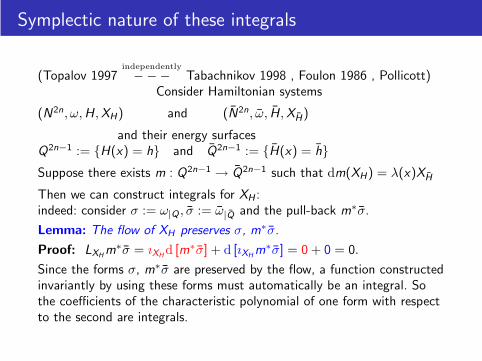
Symplectic nature of these integrals

(Topalov 1997independently

−−− Tabachnikov 1998 , Foulon 1986 , Pollicott)Consider Hamiltonian systems

(N2n, ω,H,XH) and (N2n, ω, H,XH)

and their energy surfacesQ2n−1 := {H(x) = h} and Q2n−1 := {H(x) = h}Suppose there exists m : Q2n−1 → Q2n−1 such that dm(XH) = λ(x)XH

Then we can construct integrals for XH :indeed: consider σ := ω|Q , σ := ω|Q and the pull-back m∗σ.

Lemma: The flow of XH preserves σ, m∗σ.

Proof: LXHm∗σ = ıXH

d [m∗σ] + d [ıXHm∗σ] = 0 + 0 = 0.

Since the forms σ, m∗σ are preserved by the flow, a function constructedinvariantly by using these forms must automatically be an integral. Sothe coefficients of the characteristic polynomial of one form with respectto the second are integrals.

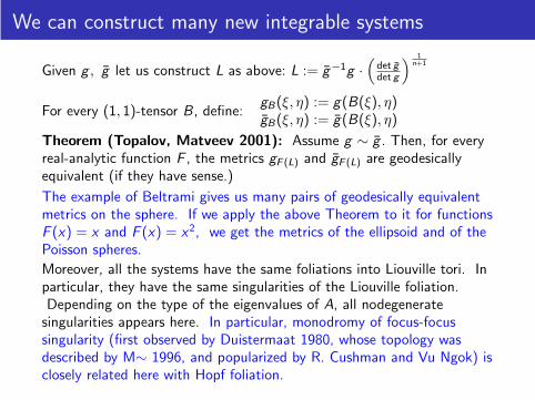
We can construct many new integrable systems

Given g , g let us construct L as above: L := g−1g ·(

det gdet g

) 1n+1

For every (1, 1)-tensor B, define:gB(ξ, η) := g(B(ξ), η)gB(ξ, η) := g(B(ξ), η)

Theorem (Topalov, Matveev 2001): Assume g ∼ g . Then, for everyreal-analytic function F , the metrics gF (L) and gF (L) are geodesicallyequivalent (if they have sense.)

The example of Beltrami gives us many pairs of geodesically equivalentmetrics on the sphere. If we apply the above Theorem to it for functionsF (x) = x and F (x) = x2, we get the metrics of the ellipsoid and of thePoisson spheres.

Moreover, all the systems have the same foliations into Liouville tori. Inparticular, they have the same singularities of the Liouville foliation.Depending on the type of the eigenvalues of A, all nodegenerate

singularities appears here. In particular, monodromy of focus-focussingularity (first observed by Duistermaat 1980, whose topology wasdescribed by M∼ 1996, and popularized by R. Cushman and Vu Ngok) isclosely related here with Hopf foliation.

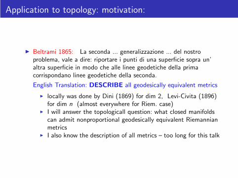
Application to topology: motivation:

◮ Beltrami 1865: La seconda ... generalizzazione ... del nostroproblema, vale a dire: riportare i punti di una superficie sopra un’altra superficie in modo che alle linee geodetiche della primacorrispondano linee geodetiche della seconda.

English Translation: DESCRIBE all geodesically equivalent metrics

◮ locally was done by Dini (1869) for dim 2, Levi-Civita (1896)for dim n (almost everywhere for Riem. case)

◮ I will answer the topologicall question: what closed manifoldscan admit nonproportional geodesically equivalent Riemannianmetrics

◮ I also know the description of all metrics – too long for this talk

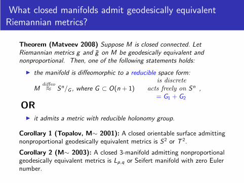
What closed manifolds admit geodesically equivalentRiemannian metrics?

Theorem (Matveev 2008) Suppose M is closed connected. LetRiemannian metrics g and g on M be geodesically equivalent andnonproportional. Then, one of the following statements holds:

◮ the manifold is diffeomorphic to a reducible space form:

Mdiffeo≈ Sn/G , where G ⊂ O(n + 1)

is discrete

acts freely on Sn

= G1 + G2

,

OR◮ it admits a metric with reducible holonomy group.

Corollary 1 (Topalov, M∼ 2001): A closed orientable surface admittingnonproportional geodesically equivalent metrics is S2 or T 2.

Corollary 2 (M∼ 2003): A closed 3-manifold admitting nonproportionalgeodesically equivalent metrics is Lp,q or Seifert manifold with zero Eulernumber.

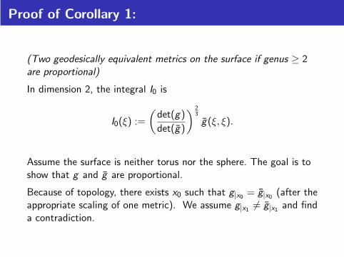
Proof of Corollary 1:

(Two geodesically equivalent metrics on the surface if genus ≥ 2are proportional)

In dimension 2, the integral I0 is

I0(ξ) :=

(det(g)

det(g)

) 23

g(ξ, ξ).

Assume the surface is neither torus nor the sphere. The goal is toshow that g and g are proportional.

Because of topology, there exists x0 such that g|x0= g|x0

(after theappropriate scaling of one metric). We assume g|x1

6= g|x1and find

a contradiction.

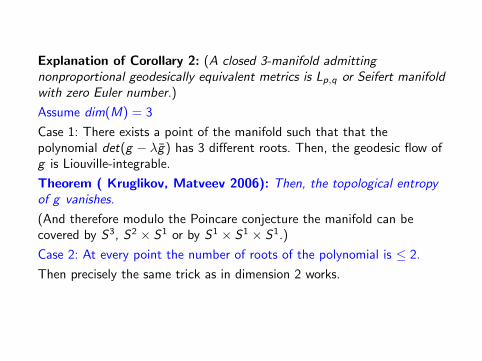
Explanation of Corollary 2: (A closed 3-manifold admittingnonproportional geodesically equivalent metrics is Lp,q or Seifert manifoldwith zero Euler number.)

Assume dim(M) = 3

Case 1: There exists a point of the manifold such that that thepolynomial det(g − λg) has 3 different roots. Then, the geodesic flow ofg is Liouville-integrable.

Theorem ( Kruglikov, Matveev 2006): Then, the topological entropyof g vanishes.

(And therefore modulo the Poincare conjecture the manifold can becovered by S3, S2 × S1 or by S1 × S1 × S1.)

Case 2: At every point the number of roots of the polynomial is ≤ 2.

Then precisely the same trick as in dimension 2 works.

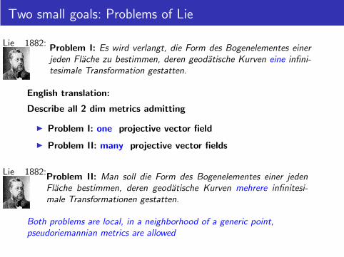
Two small goals: Problems of Lie

Lie 1882:Problem I: Es wird verlangt, die Form des Bogenelementes einerjeden Flache zu bestimmen, deren geodatische Kurven eine infini-tesimale Transformation gestatten.

English translation:

Describe all 2 dim metrics admitting

◮ Problem I: one projective vector field

◮ Problem II: many projective vector fields

Lie 1882:Problem II: Man soll die Form des Bogenelementes einer jedenFlache bestimmen, deren geodatische Kurven mehrere infinitesi-male Transformationen gestatten.

Both problems are local, in a neighborhood of a generic point,pseudoriemannian metrics are allowed

Solution of the 2nd Lie Problem

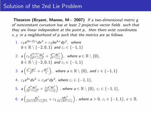
Theorem (Bryant, Manno, M∼ 2007) If a two-dimensional metric gof nonconstant curvature has at least 2 projective vector fields such thatthey are linear independent at the point p, then there exist coordinatesx , y in a neighborhood of p such that the metrics are as follows.

1. ε1e(b+2) xdx2 + ε2beb xdy2, where

b ∈ R \ {−2, 0, 1} and εi ∈ {−1, 1}

2. a(

ε1e(b+2) xdx2

(eb x+ε2)2 + eb xdy2

eb x+ε2

)

, where a ∈ R \ {0},b ∈ R \ {−2, 0, 1} and εi ∈ {−1, 1}

3. a(

e2 xdx2

x2 + ε dy2

x

)

, where a ∈ R \ {0}, and ε ∈ {−1, 1}

4. ε1e3xdx2 + ε2e

xdy2, where εi ∈ {−1, 1},

5. a(

e3xdx2

(ex+ε2)2 + ε1exdy2

(ex+ε2)

)

, where a ∈ R \ {0}, εi ∈ {−1, 1},

6. a(

dx2

(cx+2x2+ε2)2x+ ε1

xdy2

cx+2x2+ε2

)

, where a > 0, εi ∈ {−1, 1}, c ∈ R.

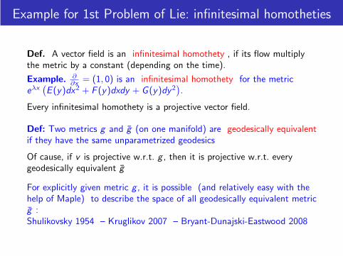
Example for 1st Problem of Lie: infinitesimal homotheties

Def. A vector field is an infinitesimal homothety , if its flow multiplythe metric by a constant (depending on the time).

Example. ∂∂x

= (1, 0) is an infinitesimal homothety for the metriceλx

(E (y)dx2 + F (y)dxdy + G (y)dy2

).

Every infinitesimal homothety is a projective vector field.

Def: Two metrics g and g (on one manifold) are geodesically equivalentif they have the same unparametrized geodesics

Of cause, if v is projective w.r.t. g , then it is projective w.r.t. everygeodesically equivalent g

For explicitly given metric g , it is possible (and relatively easy with thehelp of Maple) to describe the space of all geodesically equivalent metricg :Shulikovsky 1954 – Kruglikov 2007 – Bryant-Dunajski-Eastwood 2008

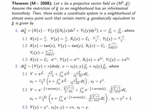
Theorem (M∼ 2008): Let v be a projective vector field on (M2, g).Assume the restriction of g to no neighborhood has an infinitesimalhomothety. Then, there exists a coordinate system in a neighborhood ofalmost every point such that certain metric g geodesically equivalent tog is given by

1. ds2g = (X (x) − Y (y))(X1(x)dx2 + Y1(y)dy2), v = ∂

∂x+ ∂

∂y, where

1.1 X (x) = 1x, Y (y) = 1

y, X1(x) = C1 · e−3x

x, Y1(y) = e−3y

y.

1.2 X (x) = tan(x), Y (y) = tan(y), X1(x) = C1 · e−3λx

cos(x) ,

Y1(y) = e−3λy

cos(y) .

1.3 X (x) = C1 · eνx , Y (y) = eνy , X1(x) = e2x , Y1(y) = ±e2y .

2. ds2g = (Y (y) + x)dxdy , v = v1(x , y) ∂

∂x+ v2(y) ∂

∂y, where

2.1 Y = e32y ·

√y

y−3 +∫ y

y0e

32ξ ·

√ξ

(ξ−3)2 dξ,

v1 = y−32

(

x +∫ y

y0e

32ξ ·

√ξ

(ξ−3)2 dξ)

, v2 = y2.

2.2 Y = e−32 λ arctan(y) ·

4√

y2+1

y−3λ +∫ y

y0e−

32 λ arctan(ξ) ·

4√

ξ2+1

(ξ−3λ)2 dξ,

v1 = y−3λ2

(

x +∫ y

y0e−

32 λ arctan(ξ) ·

4√

ξ2+1

(ξ−3λ)2 dξ

)

, v2 = y2 + 1.

2.3 Y (y) = yν , v1(x , y) = νx , v2 = y .

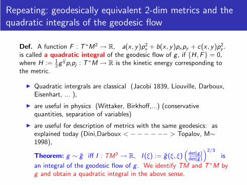
Repeating: geodesically equivalent 2-dim metrics and thequadratic integrals of the geodesic flow

Def. A function F : T ∗M2 → R, a(x , y)p2x + b(x , y)pxpy + c(x , y)p2

y .is called a quadratic integral of the geodesic flow of g , if {H,F} = 0,where H := 1

2g ijpipj : T ∗M → R is the kinetic energy corresponding tothe metric.

◮ Quadratic intergrals are classical (Jacobi 1839, Liouville, Darboux,Eisenhart, ... ),

◮ are useful in physics (Wittaker, Birkhoff,...) (conservativequantities, separation of variables)

◮ are useful for description of metrics with the same geodesics: asexplained today (Dini,Darboux < −−−−−− > Topalov, M∼1998),

Theorem: g ∼ g iff I : TM2 → R, I (ξ) := g(ξ, ξ)(

det(g)det(g)

)2/3

is

an integral of the geodesic flow of g . We identify TM and T ∗M byg and obtain a quadratic integral in the above sense.

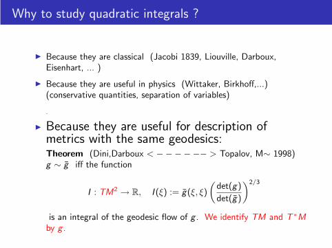
Why to study quadratic integrals ?

◮ Because they are classical (Jacobi 1839, Liouville, Darboux,Eisenhart, ... )

◮ Because they are useful in physics (Wittaker, Birkhoff,...)(conservative quantities, separation of variables)

.

◮ Because they are useful for description ofmetrics with the same geodesics:Theorem (Dini,Darboux < −−−−−− > Topalov, M∼ 1998)g ∼ g iff the function

I : TM2 → R, I (ξ) := g(ξ, ξ)

(det(g)

det(g)

)2/3

is an integral of the geodesic flow of g . We identify TM and T ∗Mby g .

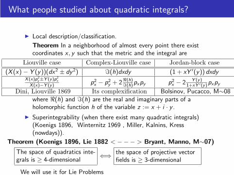
What people studied about quadratic integrals?

◮ Local description/classification.

Theorem In a neighborhood of almost every point there existcoordinates x , y such that the metric and the integral are

Liouville case Complex-Liouville case Jordan-block case

(X (x) − Y (y))(dx2 ± dy2) ℑ(h)dxdy (1 + xY ′(y)) dxdyX (x)p2

y±Y (y)p2x

X (x)−Y (y) p2x − p2

y + 2ℜ(h)ℑ(h)pxpy p2

x − 2 Y (y)1+xY ′(y)pxpy

Dini, Liouville 1869 Its complexification Bolsinov, Pucacco, M∼08

where ℜ(h) and ℑ(h) are the real and imaginary parts of aholomorphic function h of the variable z := x + i · y .

◮ Superintegrability (when there exist many quadratic integrals)(Koenigs 1896, Winternitz 1969 , Miller, Kalnins, Kress(nowdays)).

Theorem (Koenigs 1896, Lie 1882 < −−− > Bryant, Manno, M∼07)

The space of quadratics inte-grals is ≥ 4-dimensional

⇐⇒ the space of projective vectorfields is ≥ 3-dimensional

We will use it for Lie Problems

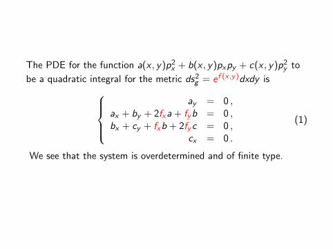
The PDE for the function a(x , y)p2x + b(x , y)pxpy + c(x , y)p2

y to

be a quadratic integral for the metric ds2g = ef (x ,y)dxdy is

ay = 0 ,ax + by + 2fxa + fyb = 0 ,bx + cy + fxb + 2fyc = 0 ,

cx = 0 .

(1)

We see that the system is overdetermined and of finite type.

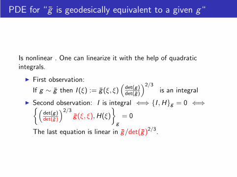
PDE for “g is geodesically equivalent to a given g“

Is nonlinear . One can linearize it with the help of quadraticintegrals.

◮ First observation:

If g ∼ g then I (ξ) := g(ξ, ξ)(

det(g)det(g)

)2/3is an integral

◮ Second observation: I is integral ⇐⇒ {I , H}g = 0 ⇐⇒{(

det(g)det(g)

)2/3g(ξ, ξ), H(ξ)

}

g

= 0

The last equation is linear in g/det(g)2/3.

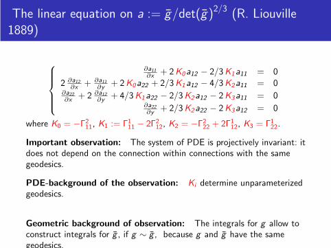
The linear equation on a := g/det(g)2/3 (R. Liouville1889)

∂a11

∂x+ 2K0a12 − 2/3K1a11 = 0

2 ∂a12

∂x+ ∂a11

∂y+ 2K0a22 + 2/3K1a12 − 4/3K2a11 = 0

∂a22

∂x+ 2 ∂a12

∂y+ 4/3K1a22 − 2/3K2a12 − 2K3a11 = 0

∂a22

∂y+ 2/3K2a22 − 2K3a12 = 0

where K0 = −Γ211, K1 := Γ1

11 − 2Γ212, K2 = −Γ2

22 + 2Γ112, K3 = Γ1

22.

Important observation: The system of PDE is projectively invariant: itdoes not depend on the connection within connections with the samegeodesics.

PDE-background of the observation: Ki determine unparameterizedgeodesics.

Geometric background of observation: The integrals for g allow toconstruct integrals for g , if g ∼ g , because g and g have the samegeodesics.

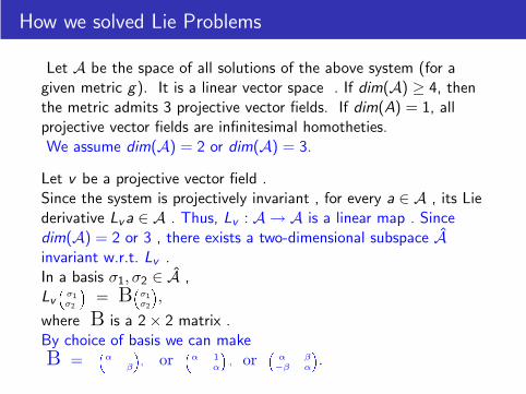
How we solved Lie Problems

Let A be the space of all solutions of the above system (for agiven metric g). It is a linear vector space . If dim(A) ≥ 4, thenthe metric admits 3 projective vector fields. If dim(A) = 1, allprojective vector fields are infinitesimal homotheties.We assume dim(A) = 2 or dim(A) = 3.

Let v be a projective vector field .Since the system is projectively invariant , for every a ∈ A , its Liederivative Lva ∈ A . Thus, Lv : A → A is a linear map . Sincedim(A) = 2 or 3 , there exists a two-dimensional subspace Ainvariant w.r.t. Lv .In a basis σ1, σ2 ∈ A ,Lv

�σ1σ2

�= B

�σ1σ2

�,

where B is a 2 × 2 matrix .By choice of basis we can makeB =

�α

β

�, or

�α 1

α

�, or

�α β

−β α

�.

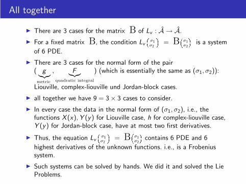
All together

◮ There are 3 cases for the matrix B of Lv : A → A.

◮ For a fixed matrix B, the condition Lv

�σ1σ2

�= B

�σ1σ2

�is a system

of 6 PDE.

◮ There are 3 cases for the normal form of the pair( g︸︷︷︸

metric

, F︸︷︷︸

quadratic integral

) (which is essentially the same as (σ1, σ2)):

Liouville, complex-liouville und Jordan-block cases.

◮ all together we have 9 = 3 × 3 cases to consider.

◮ In every case the data in the normal form of (σ1, σ2), i.e., thefunctions X (x),Y (y) for Liouville case, h for complex-liouville case,Y (y) for Jordan-block case, have at most two first derivatives.

◮ Thus, the equation Lv

�σ1σ2

�= B

�σ1σ2

�contains 6 PDE and 6

highest derivatives of the unknown functions. i.e., is a Frobeniussystem.

◮ Such systems can be solved by hands. We did it and solved the LieProblems.

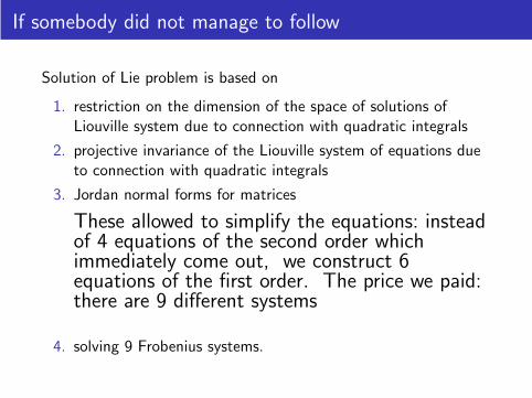
If somebody did not manage to follow

Solution of Lie problem is based on

1. restriction on the dimension of the space of solutions ofLiouville system due to connection with quadratic integrals

2. projective invariance of the Liouville system of equations dueto connection with quadratic integrals

3. Jordan normal forms for matrices

These allowed to simplify the equations: insteadof 4 equations of the second order whichimmediately come out, we construct 6equations of the first order. The price we paid:there are 9 different systems

4. solving 9 Frobenius systems.

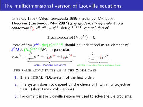
The multidimensional version of Liouville equations

Sinjukov 1962/ Mikes, Berezovski 1989 / Bolsinov, M∼ 2003.Theorem (Eastwood, M∼ 2007) g is geodesically equivalent to aconnection Γi

jk iff σab := g ab · det(g)1/(n+1) is a solution of

Tracefreepartof(∇aσ

bc)

= 0.

Here σab := g ab · det(g)1/(n+1) should be understood as an element ofS2M ⊗ (Λn)

2/(n+1)M. In particular,

∇aσbc =

∂

∂xaσbc + Γb

adσdc + Γcdaσ

bd

︸ ︷︷ ︸

Usual covariant derivative

− 2

n + 1Γd

da σbc

︸ ︷︷ ︸

addition coming from volume form

The same advantages as in the 2-dim case:

1. It is a linear PDE-system of the first order.

2. The system does not depend on the choice of Γ within a projectiveclass. (short tensor calculations)

3. For dim2 it is the Liouville system we used to solve the Lie problems.

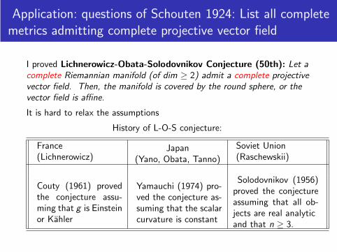
Application: questions of Schouten 1924: List all completemetrics admitting complete projective vector field

I proved Lichnerowicz-Obata-Solodovnikov Conjecture (50th): Let acomplete Riemannian manifold (of dim ≥ 2) admit a complete projectivevector field. Then, the manifold is covered by the round sphere, or thevector field is affine.

It is hard to relax the assumptions

History of L-O-S conjecture:

France(Lichnerowicz)

Japan(Yano, Obata, Tanno)

Soviet Union(Raschewskii)

Couty (1961) provedthe conjecture assu-ming that g is Einsteinor Kahler

Yamauchi (1974) pro-ved the conjecture as-suming that the scalarcurvature is constant

Solodovnikov (1956)proved the conjectureassuming that all ob-jects are real analyticand that n ≥ 3.

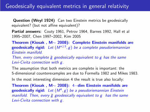
Geodesically equivalent metrics in general relativity

Question (Weyl 1924) Can two Einstein metrics be geodesicallyequivalent? (but not affine equivalent)?

Partial answers: Couty 1961, Petrov 1964, Barnes 1992, Hall et al1995–2007, Chen 1997–2002, Kim 2005

Theorem (Kiosak , M∼ 2008): Complete Einstein manifolds aregeodesically rigid: Let (Mn≥3, g) be a complete pseudoriemannianEinstein manifold.Then, every complete g geodesically equivalent to g has the sameLevi-Civita connection with g.

The assumption that both metrics are complete is important: the5-dimensional counterexamples are due to Formella 1982 and Mikes 1983.

In the most interesting dimension 4 the result is true also locally:

Theorem (Kiosak , M∼ 2008): 4−dim Einstein manifolds aregeodesically rigid: Let (M4, g) be a pseudoriemannian Einsteinmanifold. Then, every g geodesically equivalent to g has the sameLevi-Civita connection with g.

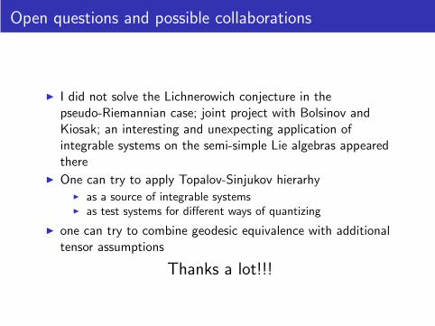
Open questions and possible collaborations

◮ I did not solve the Lichnerowich conjecture in thepseudo-Riemannian case; joint project with Bolsinov andKiosak; an interesting and unexpecting application ofintegrable systems on the semi-simple Lie algebras appearedthere

◮ One can try to apply Topalov-Sinjukov hierarhy◮ as a source of integrable systems◮ as test systems for different ways of quantizing

◮ one can try to combine geodesic equivalence with additionaltensor assumptions

Thanks a lot!!!