WISSENSCHAFTSZENTRUM BERLIN FÜR SOZIALFORSCHUNG SOCIAL SCIENCE RESEARCH CENTER BERLIN

Vivek Ghosal *

Impact of Uncertainty and Sunk Costs on Firm Survival and Industry Dynamics

* Georgia Institute of Technology

SP II 2003 – 12

August 2003

ISSN Nr. 0722 – 6748

Research Area Markets and Political Economy

Research Unit Competitiveness and Industrial Change

Forschungsschwerpunkt Markt und politische Ökonomie

Abteilung Wettbewerbsfähigkeit und industrieller Wandel

Zitierweise/Citation: Vivek Ghosal, Impact of Uncertainty and Sunk Costs on Firm Survival and Industry Dynamics, Discussion Paper SP II 2003 – 12, Wissenschaftszentrum Berlin, 2003. Wissenschaftszentrum Berlin für Sozialforschung gGmbH, Reichpietschufer 50, 10785 Berlin, Germany, Tel. (030) 2 54 91 – 0 Internet: www.wz-berlin.de

ii

ABSTRACT

Impact of Uncertainty and Sunk Costs on Firm Survival and Industry Dynamics

by Vivek Ghosal*

This paper examines the role played by uncertainty and sunk costs on the time-series fluctuations in industry structure as captured by the number of firms and establishments, and concentration. Using an extensive dataset covering 267 U.S. manufacturing industries over a 30-year period, our estimates show that time periods of greater uncertainty, especially in conjunction with higher sunk costs, results in: (i) decrease in the number of small firms and establishments; (ii) less skewed size distribution of firms and establishments; and (iii) marginal increase in industry output concentration. Large establishments are virtually unaffected. We also control for technological change and our estimates show that technical progress decreases the number of small firms and establishments in an industry. While past studies have emphasized technological change as a key driver of industry dynamics, our results indicate that uncertainty and sunk costs play a crucial role. Our findings could be useful for competition policy, study of firm survival, models of creative destruction, evolution of firm size distribution, and mergers and acquisitions. Keywords: Industry dynamics, firm survival, firm size distribution, uncertainty, sunk

costs, technological change, creative destruction, option value, financing constraints.

JEL Classification: L11, D80, O30, G10, L40.

* For helpful comments and discussions on earlier versions, I thank Bob Chirinko,

Andrew Dick, Ciaran Driver, Michael Funke, Boyan Jovanovic, Steven Klepper, Alex Raskovich, Dave Reitman, Mark Roberts, Mary Sullivan and seminar participants at the following conferences and universities: “New Perspectives on Fixed Investment” organized by the City University of London Business School, North American Econometric Society, European Network on Industrial Policy, Royal Economic Society, International Schumpeter Society, European Association for Research in Industrial Economics, “The Economics of Entrepreneurship and the Demography of Firms and Industries” organized by Zentrum für Europäische Wirtschaftsforschung (ZEW, Mannheim), “Post-Entry Performance of Firms: Role of Technology, Growth and Survival” organized by the University of Bologna, CESifo (Munich) Area Conference in Industrial Organization, Catholic University of Leuven, City University of New York, Tilburg University, New York University and University of Florida. Finally, parts of this paper were completed when I was a research visitor at the Central Planning Bureau (The Hague, Netherlands) and the Wissenschaftszentrum Berlin für Sozialforschung (WZB); I thank them for providing research support and their hospitality.

iii

ZUSAMMENFASSUNG

Die Bedeutung von Unsicherheit und 'sunk costs' für das Überleben von Unternehmen und die Weiterentwicklung von Industrien

In diesem Diskussionspapier wird die Rolle untersucht, die Unsicherheit und ‚sunk costs’ auf die Zeitreihenfluktuationen in der Industriestruktur, wie sie durch die Anzahl der Unternehmen abgebildet wird, und in der Unternehmenskonzentration haben. Dafür wird ein umfassender Datensatz verwendet, der 267 Firmen des verarbeitenden Gewerbes in den U.S.A. über einen Zeitraum von 30 Jahren enthält. Unsere Schätzungen zeigen, daß sich Zeiten größerer Ungewißheit auf die Industrie auswirken, vor allem wenn die Unsicherheit mit höheren sunk-costs verbunden ist, indem (i) die Zahl kleinerer Unternehmen abnimmt; (ii) die Verteilung der Unternehmen nach ihrer Größe weniger schief-verteilt ist; und (iii) ein Grenzzuwachs an Outputkonzentration der Industrie zu verzeichnen ist. Große Einrichtungen bleiben dagegen nahezu unberührt. Wir habe unsere Untersuchung darüberhinaus auf technologischen Wandel hin kontrolliert und festgestellt, daß die technische Weiterentwicklung die Zahl der kleinen Unternehmen eines Industriezweigs ebenfalls reduziert. Während frühere Studien gerade den technologischen Wandel als den treibenden Faktor für die dynamische Entwicklung von Industrien herausgestellt haben, weisen unsere Ergebnisse allerdings den Faktoren Unsicherheit und ‚sunk-costs’ die entscheidende Rolle zu. Diese Ergebnisse können fruchtbar für weitere Studien im Bereich der Wettbewerbspolitik sein, für Studien zum Überleben von Firmen, für Modelle kreativer Zerstörung, der Evolution von Firmengrößenverteilung und nicht zuletzt für Unternehmensaufkäufe und -zusammenschlüsse (M&A).

iv

1 Sutton (1997.a; p.52-54) writes that fluctuations in industry profits influence entry and exit, and (p.53) “a newattack on this problem has been emerging recently, following the work of Avinash Dixit and Robert Pindyck (1994)on investment under uncertainty. Here, the focus is on analyzing the different thresholds associated with entrydecisions which involve sunk costs and decisions to exit...”

1

I. Introduction

Several stylized facts are well established (Caves, 1998; Sutton, 1997a): (i) there is significant turnover of

firms in mature industries; (ii) the typical entering (exiting) firm is small compared to incumbents; and (iii)

incumbent larger firms are older with higher survival probabilities. Given these findings, it is crucial to

identify the forces that drive intertemporal dynamics of industry structure and the evolution of firm size

distribution. Starting with Gort and Klepper (1982), much of the literature has focused on technological

change as a key factor driving industry life-cycles and turnover in mature industries (Audretsch, 1995;

Caves, 1998; Sutton, 1997a). However, other key forces identified in theory have been somewhat neglected

in the empirical literature. The primary objective of this paper is to provide an understanding of the role

played by uncertainty and sunk costs on the time-series variations in the number of firms and establishments,

and concentration, in relatively mature industries.

The primary channel we examine relates to uncertainty and sunk costs which imply an option value

of waiting and alter the entry/exit trigger prices (Dixit, 1989; Dixit and Pindyck, 1994). This suggests that

uncertainty and sunk costs are likely to be an important determinant of the intertemporal dynamics of

industry structure (Section II(i)). Our study is motivated by the fact that while the theory is well developed,

empirical evaluation of these models appears limited.1 A potentially second channel is financial market

frictions (Cooley and Quadrini, 2001; Cabral and Mata, 2003; Greenwald and Stiglitz, 1990; Williamson,

1988). This literature suggests that uncertainty and sunk costs, among other factors, exacerbate financing

constraints, which may affect decisions of entrants and incumbents and shape industry dynamics (Section

II(ii)). Finally, following the previous literature, we examine other forces, including technology, that may

drive industry dynamics (Section III).

Our empirical analysis is conducted using a within-industry time-series framework. We assembled

an extensive database covering 267 SIC 4-digit manufacturing industries over 1958-92, with data on the

number of firms and establishments (by size groups), output concentration, alternative proxies for sunk

capital costs, and use time-series data to measure uncertainty and technical change (Section IV). We use a

dynamic panel data model to estimate the impact of uncertainty on the intertemporal dynamics of industry

structure (Section V). Our estimates (Section VI) show that periods of greater uncertainty, especially in

conjunction with higher sunk costs, result in: (i) reduction in the number of small establishments and firms;

(ii) less skewed size distribution of firms, and (iii) marginally higher industry concentration. Large

2 Hopenhayn (1992), Lambson (1991) and Pakes and Ericsson (1998), e.g., study firm dynamics assuming firm-specific uncertainty. The latter also evaluate models of firm dynamics under active v. passive learning. Thesemodels can be better subjected to empirical evaluation using micro-datasets, as in Pakes and Ericsson.

2

establishments are virtually unaffected. Second, technological progress has an adverse impact on the number

of small firms and establishments in an industry - a finding similar to Audretsch (1995).

Our findings could be useful in several areas. First, they may provide guidance for competition

policy since analysis of entry is an integral part of DOJ/FTC merger guidelines. Sunk costs are explicitly

discussed as a barrier to entry, but uncertainty is de-emphasized. Our results suggest that uncertainty

compounds the sunk cost barriers, retards entry and lowers the survival probability of smaller incumbents;

thus, uncertainty could be an added consideration in the forces governing market structure. Second,

determinants of M&A activity is an important area of research; see Jovanovic and Rousseau (2001) and the

references there. If periods of greater uncertainty lowers the probability of survival and increases exits, it

may have implications for reallocation of capital; do the assets exit the industry or are they reallocated via

M&A? It may be useful to explore whether uncertainty helps explain part of M&A waves. Third, while

skewed firm size distribution is well documented, empirical analysis of the determinants of it’s evolution

is limited. Our results suggest that periods of greater uncertainty, in conjunction with sunk costs, may play

a role. Fourth, Davis, et al. (1996) find that job destruction/creation decline with firm size/age; Cooley and

Quadrini (2001) and Cabral and Mata (2001) suggest that small firms may have greater destruction (exits)

due to financial frictions. Our results provide additional insights: periods of greater uncertainty, in

combination with higher sunk costs, appear to significantly influence small firm turnover. Finally, they

could provide insights into the evolution of specific industries: e.g., the U.S. electric industry is undergoing

deregulation and we are observing numerous mergers involving firms of different sizes. Also, uncertainty

about prices and profits are well documented resulting in utilities experiencing financial distress. Our

findings could predict a future path that leads to greater concentration and weeding out of smaller firms.

II. Uncertainty and Sunk Costs

II(i). Option Value

Dixit (1989), Dixit and Pindyck (1994) and Caballero and Pindyck (1996) provide a broad framework to

study time-series variations in entry, exit and the number of firms.2 To streamline our discussion, we

introduce some notation. As in the above models, let S(K) be sunk costs, which are assumed proportional

to the entry capital requirement; Z the stochastic element with the conditional standard deviation of Z, F(Z),

measuring uncertainty; and PH and PL the entry and exit trigger prices - over (0,PH) the potential entrant

3

holds on to its option to enter, and over (PL,4) an incumbent does not exit. Dixit (1989) shows that

uncertainty and sunk costs imply an option value of waiting for information and this raises PH and lowers

PL. During periods of greater uncertainty, entry is delayed as firms require a premium over the conventional

Marshallian entry price, and exit is delayed as incumbents know they have to re-incur sunk costs upon re-

entry. Caballero and Pindyck (1996) model the intertemporal path of a competitive industry where negative

demand shocks decrease price along existing supply curve, but positive shocks may induce entry/expansion

by incumbents, shifting the supply curve to the right and dampening price increase. Since the upside is

truncated by entry but the downside is unaffected, it reduces the expected payoff from investment and raises

the entry trigger. If exit is likely, it would create a price floor making firms willing to accept a period of

losses. Their data on SIC 4-digit manufacturing industries (similar to ours) shows that sunk costs and

industry-wide uncertainty cause the entry (investment) trigger to exceed the cost of capital.

For our empirical analysis, we would like to know whether during periods of greater F(Z), is PH

affected more than PL or vice versa? General analytic answers are difficult to obtain. But numerical

simulations in Dixit and Pindyck (Ch. 7, 8) show that increase in F(Z) given S(K) - or increase in S(K)

given F(Z) - results in PH increasing by more than the decrease in PL; Figure 1 (a, b) illustrates this. This

implies that during periods of greater uncertainty, entry is affected more than exit leading to negative net

entry; i.e., an industry is likely to show a decrease in the number of firms.

Turning to imperfect competition, first consider a duopoly setting (Dixit and Pindyck, p.309-315).

Entry price exceeds the Marshallian trigger due to uncertainty and sunk costs, preserving the option value

of waiting. But, there are strategic considerations. Under simultaneous decision making, when price is ,

above the entry trigger, neither firm wants to wait for fear of being preempted by its rival and losing

leadership. This could lead to faster, simultaneous, entry than in the leader-follower sequential entry setting.

Thus fear of pre-emption may necessitate a faster response and counteract the option value of waiting.

Second, Appelbaum and Lim (1985), Dixit (1980) and Spencer and Brander (1992) demonstrate the

optimality of strategic pre-commitment by the incumbent/first-mover. But under uncertainty, optimal pre-

commitment is lower due to greater uncertainty about the success of the entry-deterring strategy.

Oligopolistic settings, therefore, highlight the dependence of outcomes on model assumptions and

difficulties of arriving at clear predictions.

Links to Empirical Analysis

Following the framework provided by theory, our empirical analysis will examine time-series variation in

industry structure variables; e.g., the number of firms. Before summarizing the predictions, we note two

3 See Audretsch (1995), Dunne et al. (1988), Evans (1987) and Sutton (1997.a). In Audretsch (p.73-80), meansize of the entering firm is 7 employees, varying from 4 to 15 across 2-digit industries. Audretsch (p.159) finds19% of exiting firms have been in the industry less than 2 years with mean size of 14 employees; for exiting firmsof all ages, the mean size is 23. Dunne et al. (p.503) note that about 39% of firms exit from one Census to the nextand entry cohort in each year accounts for about 16% of an industry’s output.” While the number of entrants islarge, their size is tiny relative to incumbents. Data indicate similar pattern for exiters.

4 Cable and Schwalbach (1991), Dunne, Roberts and Samuelson (1988), Evans and Siegfried (1994) andGeroski (1995). For SIC 4-digit industries over the 1963-82 Censuses (similar to ours), Dunne et al. find rawcorrelations between entry and exit rates of 0.18 to 0.33; while positive, they are relatively low implyingconsiderable variation in net entry patterns across industries. Also, after sweeping out industry fixed-effects, thecorrelations turn negative (-0.028 to -0.249) overturning inference from raw data.

4

issues. First, within-industry firm size distribution is typically skewed (Ijiri and Simon, 1977; Sutton,

1997.a). Our data (Section IV(i)) reveals this to be the typical characteristic. Previous studies show that (i)

entrants are typically small compared to incumbents and have high failure rates, (ii) typical exiting firm is

small and young, and (iii) larger firms are older with higher survival rates.3 We address the small v. large

firm issue in our empirical analysis. Second, our SIC 4-digit manufacturing industry data, which cover a 30-

year span, contains information on the total number of firms and establishments (by size class) in an

industry. Several studies have noted a positive correlation between entry and exit rates; however, these

correlations are not necessarily contemporaneous and the studies indicate wide cross-industry variation in

patterns of net entry.4 In Section IV(i) we show that our data contains reasonable within-industry time-series

variation in net entry, which is encouraging for our empirical analysis.

For our within-industry time-series analysis, we summarize the implications as follows:

(A) Net entry. We noted that periods of greater F(Z) are likely to result in negative net entry. Would small

v. large firms be affected differentially? Large firms are older and have “cumulatively” greater investments

in, e.g., advertising and R&D; see Sutton (1991, 1997.b) and Caves (1998). Advertizing and distribution

networks contain sunk investments which erode upon exit and would have to be re-established if the firm

re-enters in future; similarly exit entails loss of human and physical capital related to product and process

innovation. Thus, larger firms are more likely to show greater inaction regarding exit. Since data shows that

entrants are rather small, entry of large firms is typically not an important consideration. Overall, we expect

greater inaction in large firm net entry (little/no entry and lower exits) during periods of greater uncertainty.

Entry cohorts typically consist of relatively small firms, and exit cohorts of young and small firms.

Based on the results discussed earlier, periods of greater F(Z) will delay entry more than exit, resulting in

negative net entry; i.e., we can expect a decrease in the number of smaller firms. Further, based on

the predictions from theory, this effect will be exacerbated when sunk costs, S(K), are higher.

(B) Size distribution. If there is greater attrition among small firms, then firm size distribution will become

5 On asset recovery by debt holders, Williamson writes: (p.571) “Of the several dimensions with respect towhich transactions differ, the most important is the condition of asset specificity. This has a relation to the notionof sunk cost...” (p.580) “In the event of default, the debt-holders will exercise pre-emptive claims against theassets in question....The various debt holders will then realize differential recovery in the degree to which theassets in question are redeployable...the value of a pre-emptive claim declines as the degree of asset specificitydeepens...”

5

less skewed, and this effect will be more pronounced in high sunk cost industries.

(C) Concentration. Given the above, industry concentration would be expected to increase marginally since

the smaller firms typically account for a trivial share of industry output.

II(ii). Financing Constraints

Several recent studies have examined the impact of financing constraints on firm survival. Cooley and

Quadrini (2001) model industry dynamics with financial market frictions, where firms finance capital

outlays by issuing new shares or borrowing from financial intermediaries, but both are costly.

Smaller/younger firms borrow more and have higher probability of default; with increasing size/age, the

default probability falls dramatically. Due to financial frictions, smaller/younger firms have higher

probability of exit. Empirical results in Cabral and Mata (2001) suggest that financing constraints cause

lower survival probability and higher exits among small firms.

An earlier literature has examined some of the underlying factors that may contribute to financial

market frictions. First, consider uncertainty. Greenwald and Stiglitz (1990) model firms as maximizing

expected equity minus expected cost of bankruptcy and examine scenarios where firms may be equity or

borrowing constrained. A key result is that greater uncertainty about profits exacerbates information

asymmetries, tightens financing constraints and lowers capital outlays. Since uncertainty increases the risk

of bankruptcy, firms cannot issue equity to absorb the risk. Brito and Mello (1995) extend the Greenwald-

Stiglitz framework to show that small firm survival is adversely affected by financing constraints. Second,

higher sunk costs imply that lenders will be more hesitant to provide financing because asset specificity

lowers resale value implying that collateral has less value (Williamson, 1988).5 In Shleifer and Vishny

(1992), asset specificity is a determinant of leverage and explains time-series and cross-industry patterns

of financing; the ease of debt financing is inversely related to asset specificity. Lensink, Bo and Sterken

(2001) provide a lucid discussion of financing constraints in the related context of investment behavior.

In short, periods of greater uncertainty, in conjunction with higher sunk costs, increase the likelihood

of bankruptcy and exacerbate financing constraints. Incumbents who are more dependent on borrowing and

adversely affected by tighter credit are likely to have lower probability of survival and expedited 'exits'.

Firms more likely to be adversely affected are those with little/no collateral, inadequate history and shaky

6 E.g., Cabral and Mata (2003), Cooley and Quadrini (2001), Evans and Jovanovic (1989), Fazzari, et al.(1988), and Gertler and Gilchrist (1994). The latter note (p. 314): “...while size per se may not be a directdeterminant, it is strongly correlated with the primitive factors that do matter. The informational frictions thatadd to the costs of external finance apply mainly to younger firms, firms with a high degree of idiosyncratic risk,and firms that are not collateralized. These are, on average, smaller firms.”

6

past performance. Similarly, 'entry' is likely to be retarded for potential entrants who are more adversely

affected by the tighter credit conditions. Thus, periods of greater uncertainty, and in conjunction with higher

sunk costs, are likely to accelerate exits and retard entry; i.e., negative net entry.

Links to Empirical Analysis

A large literature suggests that financial market frictions are more likely to affect smaller firms.6 Using this

we postulate that small firms are more likely to be affected by financing constraints during periods of greater

uncertainty. In addition, the effect will be greater in industries with higher sunk costs.

(A) Net entry. For smaller firms, periods of greater uncertainty are likely to increase exits and lower entry;

the industry will experience loss of smaller firms. This effect will be magnified in high sunk cost industries.

(B) Size distribution. If periods of greater uncertainty cause negative net entry of smaller firms, industry firm

size distribution will become less skewed; the effect will be more pronounced under high sunk costs.

(C) Concentration. Since smaller firms are more likely to be affected, the impact on industry concentration

while positive, may not be quantitatively large.

III. Other Factors

In this section we briefly discuss some of the other factors which have been considered in the literature and

are likely to influence industry dynamics.

III(i). Technological Change

Technological change has been linked to industry life-cycle (Gort and Klepper, 1982; Jovanovic and

MacDonald, 1994) as well as ongoing turnover in relatively mature industries (Audretsch, 1995; Sutton,

1997a). While we briefly present the arguments for both, given our data we will be primarily concerned with

the latter.

Gort and Klepper (1982) examine industry life cycle and visualize two types of innovations: the

infrequent major breakthroughs that launch a new product cycle resulting in positive net entry into the

industry; and the subsequent and more frequent incremental innovations by incumbents which lead to lower

costs and weeding out of inefficient firms resulting in negative net entry. Regarding on-going incremental

7

innovations, Gort and Klepper (p.634) write:

“[this] innovation not only reinforces the barriers to entry but compresses profit margins of the lessefficient producers who are unable to imitate the leaders from among the existing firms.Consequently,...the less efficient firms are forced out of the market.”

Their data on 46 industries provides evidence of the link between technological change and net entry, with

wide inter-industry variation in patterns of evolution. Jovanovic and MacDonald (1994) provide additional

insights. These models assume low probability of successful innovations, a distribution of production

efficiency across firms, and improvements in efficiency levels due to incremental innovations, learning-by-

doing and imitation. Due to incumbents' increasing efficiency, entry is reduced to a trickle and exits continue

resulting in a reduction in the number of firms.

The above models assume convergence to steady state where industry structure becomes relatively

static. But Sutton (1997.a, p.52) notes this is at odds with observed data which show high turnover of firms

even in mature industries. Audretsch (1995), using data similar to ours, finds significant turnover in mature

industries and that industry-wide innovation (i) is negatively associated with startups and survival of new

firms and (ii) hastens small firm exit. Thus, even in mature industries, ongoing innovations are likely to play

a key role in industry dynamics. Our paper is not about studying industry life cycles, but about examining

time-series variations in the number of firms and establishments in relatively mature industries. In this sense

our focus on technology is similar to that by Audretsch. In our empirical analysis, we construct a measure

of technical change (Section IV(iv)) and examine its impact on the time-series variation of the number firms,

and small and large establishments, in an industry.

III(ii). Other Variables

We explicitly or implicitly control for some other variables that may influence industry dynamics. We

explicitly control for industry growth -GROW- and profit margins -A. Evidence on the link between

GROW and entry appears mixed. Audretsch (1995, p.61-63) finds new startups are not affected by industry

growth, but positively affected by macroeconomic growth. Data in Jovanovic and MacDonald (1994)

indicate sharp decline in the number of firms when the industry was growing. Some of the empirical papers

in Geroski and Schwalbach (1991) and the discussion in Audretsch (Ch.3) indicate a tenuous link between

GROW and industry structure. The link is likely to be conditioned on entry barriers, macroeconomic

conditions and the stage of the industry's life cycle; hence the ambiguity. Regarding profit-margin A, while

the expected sign is positive, it will be conditioned on the above mentioned factors (for GROW). Absent

entry barriers, e.g., greater A signals lucrative markets and attracts entry; but if barriers are high, the effect

is not clear. Some of the estimates presented in the papers in Geroski and Schwalbach indicate considerable

7 In Section IV(ii), following Sutton (1991), we construct a measure of minimum efficient scale (MES) for1972, ‘82 and ‘92 to proxy sunk entry costs. As noted there, the rank correlation between MES in 1972 and 1992is 0.94. This provides a basis for arguing that industry fixed-effect may capture an important part of MES.

8 We examined alternative sources. FTC Line of Business data on advertising and R&D are only available for4 years; some data are 3-digit and some 4-digit. Advertising data from the U.S. Statistics of Income: CorporateSource Book are typically at the 3-digit level and some 2-digit and there are important gaps which prevents usfrom constructing a consistent time series. Thus, these data were not useful for our long time-series study.

9 Domowitz et al. (1987) find far greater cross-industry variation in advertising than within-industry andconclude (p.25) “that by 1958, most of the industries in our sample had reached steady-state rates of advertising”This indicates that industry-fixed-effects would capture an important part of the impact of advertising.

8

variation in the coefficient of A. Geroski (1995) notes that the reaction of entry to elevated profits appears

to be slow.

For scale economies, advertizing and R&D, we don’t have explicit controls due to lack of time-series

data, but we note the following. First, our regression will contain a variable for technological change and

one could argue this captures aspects of scale economies. Second, our model includes a lagged dependent

variable; to the extent that this incorporates information on scale economies from the “recent past”, it

provides additional control. Third, scale economies are unlikely to have large short-run variations; if so, an

industry-specific constant, which we include in our dynamic panel data model, will capture aspects of this

relatively time-invariant component.7 I am not aware of SIC 4-digit time-series data on advertising or R&D

for our 267 industries over 1963-92.8 To the extent that part of R&D and advertising intensities are in steady

state levels and have a time-invariant component, this will be captured by the industry-specific constant.9

Since our empirical model includes a time-series in broad technological change, this may partly capture

R&D effects. Finally, since the lagged dependent industry structure variable captures information on

advertising and R&D from the recent past, it provides an additional control.

IV. Measurement

Our approach is as follows. First, (all variables are industry-specific): (i) we use time-series data to

create measures of uncertainty; (ii) using insights in Kessides (1990) and Sutton (1991), construct measures

of sunk costs and create low versus high sunk cost groups; and (iii) measure technological change and other

control variables. Second, following our discussion in Section II, we examine the impact of uncertainty on

the time-series variations in industry structure, as measured by the number of firms, number of small versus

large establishments, and concentration. We examine the relationship for our full sample as well as

industries segmented into low versus high sunk cost groups. Our data are at the SIC 4-digit level of

disaggregation; see Appendix A for details. An important consideration in this choice was the availability

9

of relatively long time-series which is critical for measuring uncertainty and technological change, as well

as availability of data on industry structure and sunk costs for a large number of industries over time. The

industry-specific annual time-series data are over 1958-94. Data on industry structure and sunk costs are

from the 5-yearly Census of Manufactures; these data are not available annually, implying that in our

empirical estimation we use data at a 5-yearly frequency. Below we describe the key variables.

IV(i). Industry Structure

Industry-specific time-series data from the 1963-92 Censuses include: (i) total number of firms - FIRMS;

(ii) total number of establishments - ESTB; (iii) ESTB by size classes; and (iv) four-firm concentration ratio

-CONC. Unlike ESTB, the Census does not provide data on FIRMS by size class. An establishment is an

economic entity operating at a location; as is common in the literature, we use the number of employees to

measure “size”. The Census size classes are: 1-4; 5-9; 10-19; 20-49; 50-99; 100-249; 250-499; 500-999;

1,000-2,499; and $2,500 employees. The ESTB data is used to create small v. large establishment groups.

The U.S. Small Business Administration (State of Small Business: A Report of the President, 1990), e.g.,

classifies “small business” as employing “less than 500 workers”; this has been used in public policy

initiatives and lending policies towards small businesses. Using this, <500 employees constitutes our basic

small business group, and $500 employees the large business group; Ghosal and Loungani (2000) provide

discussion of this benchmark. However, 500 employees may sometimes constitute a relatively large/wealthy

business. Since there is no well defined metric by which we can define “small”, we created additional small

business groups. Overall, our groups are: (i) All establishments; (ii) relatively large businesses with $500

employees; (iii) small businesses with <500 employees; and (iv) even smaller businesses as classified by

(a) <250, (b) <100 and (c) <50 employees. We did not push the size categories to greater extremes at either

end as this would magnify the uniqueness of the samples and render inference less meaningful.

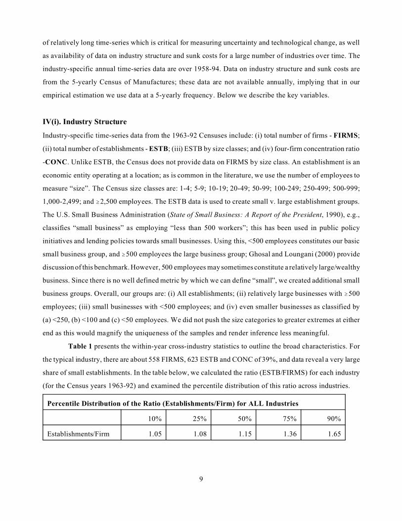
Table 1 presents the within-year cross-industry statistics to outline the broad characteristics. For

the typical industry, there are about 558 FIRMS, 623 ESTB and CONC of 39%, and data reveal a very large

share of small establishments. In the table below, we calculated the ratio (ESTB/FIRMS) for each industry

(for the Census years 1963-92) and examined the percentile distribution of this ratio across industries.

Percentile Distribution of the Ratio (Establishments/Firm) for ALL Industries

10% 25% 50% 75% 90%

Establishments/Firm 1.05 1.08 1.15 1.36 1.65

10 Since the published Census data used here does not track individual establishments over time, we are unableto directly address the issue of migration of establishments across size classes. Migration can of course take placein both directions: establishments can grow larger over time, or downsize due to changes in economic conditions,technological change, etc. These aspects can be better addressed using longitudinal data which track individualestablishments. However, we will present results on the impact of uncertainty on the “total” number of firms andestablishments in an industry (net entry effects) and this is not subject to the migration critique.

11 In the simplest settings, the theoretical models consider uncertainty about prices assuming constant inputcosts and technology. But Caballero and Pindyck (1996) and Dixit and Pindyck (1994), for example, discussuncertainty about cash-flows, profits, among other variables.

10

The number is fairly close to 1 and even at the 75th percentile level. These values imply near equivalence

between the number of establishments and firms in an industry and hence their size distributions. This

overall picture conceals a well known fact: larger (typically, older) firms tend to be multi-establishment (and

multi-product), whereas smaller (typically, newer) firms are likely to be single-establishment. For the

“representative” industry, Figures 2(a)-2(g) display data on the establishment size distribution over our

seven Census years. Typically, about 25% of the total number of establishments in an industry belong to

the smallest size category, and only about 3% belong to the largest size group. Given the statistics of the

ratio (ESTB/FIRMS), figures 2(a)-2(g) also roughly displays the size distribution of firms. The data reveals

a skewed size distribution for the typical industry as well as fluctuations in this distribution over time. The

skewed size distribution has been well documented (Ijiri and Simon, 1977; Sutton 1997.a).

Key to our empirical analysis, Table 2 presents summary statistics on the within-industry time-series

data on industry structure variables. For the “representative” industry, the mean FIRMS is 558 and within-

industry standard deviation of 129; similarly, the mean ESTB is 623 and within-industry standard deviation

of 138. In terms of sheer numbers, this time-series variation implies considerable new births and deaths of

firms and establishments. The within-industry time-series variation is encouraging for our study of the

impact of uncertainty and sunk costs on industry dynamics.10

IV(ii). Uncertainty

The stochastic element can be couched in terms of several relevant variables.11 We focus on a bottom line

measure: profit-margins. Arguably, profit-margins are important for firms making entry and exit decisions.

Commenting on the industry-specific determinants of turnover of firms, Sutton (1997.a, p.52-53) notes the

primary importance of volatility of industry profits; Dixit and Pindyck, and Caballero and Pindyck discuss

uncertainty about profits and cash-flows. We assume that firms use a profit forecasting equation to predict

the level of future profits. The forecasting equation filters out systematic components. The standard

deviation of residuals, which represent the unsystematic component (or forecast errors), measure profit-

12 E.g., Aizenman and Marion (1997), Ghosal and Loungani (1996, 2000) and Huizinga (1993) use the(conditional) standard deviation to measure uncertainty. Lensink, Bo and Sterken (2001, Ch.6) provide anextensive discussion of this and other methods that have been used to measure uncertainty.

13 This is consistent with the definition of short-run profits (Varian, 1992, Ch.2); see Domowitz et al. (1986,1987) and Machin and Van Reenen (1993) for it's empirical use. Our measure A does not control for capital costs;Carlton and Perloff (1994, p. 334-343) and Schmalensee (1989) discuss the pitfalls of alternative measures andnote that measuring capital costs is difficult due to problems related to valuing capital and depreciation.

14 Our industry level analysis implies that our procedure for measuring A and uncertainty reflects industry-wideaverage, or “typical”, outcomes. Given that there is a distribution of firm sizes, idiosyncratic uncertainty is likelyto be important and the true amount of uncertainty facing a particular firm may deviate from that for a typical firm.These issues can be better addressed using firm-level data.

15 We present some summary statistics from the regressions -equation (1)- estimated to measure uncertainty.Across the 267 industries, the mean Adjusted-R2 and the standard deviation of adjusted-R2 were 0.62 and 0.25,respectively. The first-order serial correlation was typically low, with the cross-industry mean (std. dev acrossindustries) being -0.002 (0.07). Overall, the fit of the industry regressions was reasonable.

16 We considered an alternative procedure. We used Autoregressive Conditional Heteroscedasticity (ARCH)(continued...)

11

margin uncertainty.12 We measure industry profits as short-run profits per unit of sales. Labor, energy and

intermediate materials are assumed to be the relatively variable inputs that comprise total variable costs.

Short-run profits are defined as:13 A=[(Sales Revenue minus Total Variable Costs)/(Sales Revenue)]. The

standard deviation of the unsystematic component of A measures uncertainty.14 In Section VI we construct

an alternative measure of profit-margins and uncertainty which accounts for depreciation expenditures.

For our benchmark measure of uncertainty, we use an autoregressive distributed-lag model for the

profit forecasting equation (1) which includes lagged values of A, industry-specific sales growth (SALES)

and aggregate unemployment rate (UN). The justification for this specification is contained in Domowitz,

Hubbard and Petersen (1986, 1987) and Machin and VanReenen (1993) who study the time-series

fluctuations in A. In (1), 'i' and 't' index industry and time.

Ai,t = $ + 3k2kAi,t-k + 3m.mSALESi,t-m + 3n(nUNt-n + ,i,t (1).

The following procedure is used to create a time-series for profit uncertainty: (a) for each industry, we first

estimate equation (1) using annual data over the entire sample period 1958-1994.15 The residuals represent

the unsystematic components; and (b) the standard deviation of residuals - F(A)i,t - are our uncertainty

measure. As noted earlier, industry structure data are for 1963, ‘67, ‘72, ‘77, ‘82, ‘87 and ‘92. The s.d. of

residuals over, e.g., 1967-71 serves as the uncertainty measure for 1972; similarly, s.d. of residuals over

1982-86 measures uncertainty for 1987, and so on. We get seven time-series observations on F(A)i,t.16 Table

16(...continued)models to measure uncertainty. After imposing the restrictions (Hamilton, 1994, Ch. 21), we estimated second-order ARCH for each of the 267 industries. For about 45% of the industries the estimation failed to converge;using alternative starting values, convergence criterion and order of the ARCH specification did not alleviate theproblems. This is probably not surprising given the limited number of time-series observations (36, annual) perindustry. Finally, our estimation of equation (1) over the entire sample period implies assuming stability of theparameters in (1) over the entire period. If we had longer time-series or higher frequency data (quarterly) we coulddo sub-sample estimation of (1). But due to the relatively short time series, we did not pursue this.

12

3 (col. 1) presents within-year cross-industry statistics for F(A). The s.d. is relatively high compared to the

mean value indicating large cross-industry variation. Table 4 (row 1) presents the within-industry time-

series statistics. Key to our empirical analysis, the typical industry shows a ratio of within-industry s.d.

(0.0117) to mean (0.0236) of 50%, indicating significant time-series variation in uncertainty.

When estimating (1), we initially assume k, m, n=1,2; i.e. allow for two lags of each variable. To

check for robustness, Section VI presents some additional results using alternative specifications for the

profit equation (1). These include:

(i) varying the lag length of the explanatory variables;

(ii) following Ghosal (2000) and replacing the business cycle indicator, unemployment rate, by federal funds

rate (FFR) and energy price growth (ENERGY);

(iii) estimating a basic AR(2) forecasting equation;

(iv) estimating the profit equation in growth rates instead of levels;

(v) including industry-specific cost variables; and

(vi) using an alternative measure of profit-margins that accounts for depreciation.

IV(iii). Sunk Costs

Sunk costs are notoriously difficult to measure. The literature, however, suggests some proxies. We use the

innovative framework laid out in Kessides (1990) and Sutton (1991) to quantify sunk costs. Drawing on the

contestable markets literature, Kessides (1990) notes that the extent of sunk capital outlays incurred by a

potential entrant will be determined by the durability, specificity and mobility of capital. While these

characteristics are unobservable, he constructs proxies. Let RENT denote the fraction of total capital that

a firm (entrant) can rent: RENT=(rental payments on plant and equipment/capital stock). Let USED denote

the fraction of total capital expenditures that were on used capital goods: USED=(expenditures on used plant

and equipment/total expenditures on new and used plant and equipment). Finally, let DEPR denote the share

of depreciation payments: DEPR=(depreciation payments/capital stock). High RENT implies that a greater

fraction of capital can be rented by firms (entrants), implying lower sunk costs. High USED signals active

17 RENT and USED could be useful proxies in the sense that due to the ‘lemons’ problem many types of capitalgoods suffer sharp drop in resale price in a short time period; e.g., automobile resale prices drop the most in thefirst year or two. If new entrants have access to rental or used capital, their entry capital expenditures will havea lower sunk component. We provide a couple of examples. The availability of used or leased aircraft, a prevalentfeature of that industry, makes life easier for start-up airlines. Similarly, in the oilfield drilling services industry,the key capital equipment is a mobile “rig”; a truck fitted with equipment to service the oilfields. The rigtechnology has basically been unchanged since 1979-80 and there is a large market for used and leased rigs; weobserve a rather fluid market where entrants buy or lease the used rigs.

18 Collecting these for some of the additional (and earlier) years presented particular problems due to changingindustry definitions and many missing data points.

19 E.g., (i) he assumes the K/Q ratio of the median plant is representative of the entire industry, and this isunlikely; (ii) book values are used to compute K/Q, but book values underestimate current replacement cost; (iii)the computation assumes that the age structure of capital does not vary across industries, and this is unrealistic.In addition, we note that SUNK(EC) is based on an estimate of the “median plant size” of incumbents. As notedin Section II(i), the typical entrant is small compared to incumbents, and it takes time for new entrants to attainoptimal scale. This implies that the median plant size typically overstates the entry capital requirements. Further,this bias may be greater in industries where optimal scale is relatively large, since the entrant will be farther awayfrom optimal scale; where the median plant size is small, new entrants are more likely to be closer to this size.

13

market for used capital goods which firms (entrants) have access to, implying lower sunk costs.17 High

DEPR indicates that capital decays rapidly, implying lower sunk costs (which arise from the undepreciated

portion of capital). We collected data to construct RENT, USED and DEPR for Census years 1972, 1982

and 1992.18

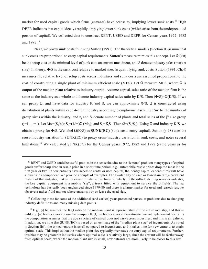
Next, we proxy sunk costs following Sutton (1991). The theoretical models (Section II) assume that

sunk costs are proportional to entry capital requirements. Sutton’s measure mimics this concept. Let M (>0)

be the setup cost or the minimal level of sunk cost an entrant must incur, and S denote industry sales (market

size). In theory, M/S is the sunk cost relative to market size. In quantifying sunk costs, Sutton (1991, Ch.4)

measures the relative level of setup costs across industries and sunk costs are assumed proportional to the

cost of constructing a single plant of minimum efficient scale (MES). Let S measure MES, where S is

output of the median plant relative to industry output. Assume capital-sales ratio of the median firm is the

same as the industry as a whole and denote industry capital-sales ratio by K/S. Then (M/S)=S(K/S). If we

can proxy S, and have data for industry K and S, we can approximate M/S. S is constructed using

distribution of plants within each 4-digit industry according to employment size. Let ‘m’ be the number of

group sizes within the industry, and nj and Sj denote number of plants and total sales of the jth size group

(j=1,...,m.). Let Msj=(Sj/nj); Se=(1/m)Gj(Msj); and So=GjSj. Then S=(Se/So). Using S and industry K/S, we

obtain a proxy for M/S. We label S(K/S) as SUNK(EC) (sunk costs-entry capital). Sutton (p.98) uses the

cross-industry variation in SUNK(EC) to proxy cross-industry variation in sunk costs, and notes several

limitations.19 We calculated SUNK(EC) for the Census years 1972, 1982 and 1992 (same years as for

20 Since cyclical utilization of inputs like capital imparts a procyclical bias to the basic Solow residual, Burnside(continued...)

14

USED, RENT and DEPR).

Sunk Cost Sub-Samples

Our approach is to create low versus high sunk cost sub-samples, and estimate the impact of uncertainty

across these groups. To create the sub-samples, we use the average values of RENT, USED and DEPR over

1972, 82 and 92; Table 5 presents the summary statistics. The measures show large cross-industry variation

given the standard deviation relative to the mean. We took a closer look at our measures for the end-points,

1972 and 1992. For the minimum efficient scale, MES, proxy S the rank correlation is 0.94 and 0.92 for

SUNK(EC), indicating fair amount of stability in the MES and SUNK(EC) measures. The mean (s.d.) for

MES and SUNK(EC) were similar over the end-points; the mean (s.d.) for USED, RENT and DEPR were

relatively similar across time. We employ two strategies to segment samples. First, we use the cross-industry

median values of each of the sunk cost proxies to create high v. low sunk cost sub-samples. If

SUNK(EC)<50th percentile, indicating relatively lower entry capital requirements, then sunk costs are low;

high if SUNK(EC)$50th percentile. Similarly, sunk costs are low if RENT or USED or DEPR $50th

percentile; high if RENT or USED or DEPR <50th percentile. Second, we created sub-samples by combining

alternative characteristics, the argument being that they may produce stronger separation between low and

high sunk costs. For example, sunk costs would be low if the intensity of rental and used capital markets

are high and depreciation is high. More specifically, low sunk costs if “USED and RENT and DEPR $50th

percentile”; high if “RENT and USED and DEPR <50th percentile”. Our final grouping is, low sunk costs

if “USED and RENT and DEPR $50th and SUNK(EC) <50th percentile”; high if “RENT and USED and

DEPR <50th percentile and SUNK(EC) $50th percentile”.

IV(iv). Other Variables

Regarding technological change, we need a time-series measure for our analysis. The previous literature has

used several measures: e.g., specific innovations for selected industries (Gort and Klepper, 1982);

commercially introduced innovations (Audretsch, 1995); and R&D and patents (Cohen and Levin, 1989).

Unfortunately, time-series data on these variables are not available for our 267 industries over the 1958-92

period (also see footnote 8). Given the data limitations, we pursue an alternative strategy and construct an

industry-specific time-series for technological change. We construct a factor-utilization-adjusted Solow

technology residual following the insights in Burnside (1996) and Basu (1996).20 Burnside (1996) assumes

20(...continued)et al. (1995) use electricity consumption to proxy utilization of capital and obtain corrected Solow residual;Burnside (1996) uses total energy consumption; and Basu (1996) materials inputs. The intuition is that materialsand energy don’t have cyclical utilization component and are good proxies for the utilization of capital; assumingconstant capital stock, if capital utilization increases, then materials and energy usage will typically increase.

21 In an alternative specification Leontief technology is assumed where gross output Q is produced withmaterials (M) and value-added (V): Q t=min("VVt, "MM t), where "’s are constants. V is produced with CRS andusing capital services (S) and labor hours (H): Vt=Zt F(Ht, St), where Z is the exogenous technology shock. Since“S” is unobserved, it is assumed proportional to electricity consumption or total energy usage (E); E= >S. Giventhis and the assumption of perfectly competitive factor markets, the factor utilization adjusted technology residualis: TECH(alt)=[ªvt - (1-"Kt)ªht - "Ktªet], where the lower-case letters denote logarithms of value-added, laborhours and energy. Using this approach to measure the technology residual did not alter our inferences.

22 In theory, an entrant should rationally expect profit-margins to fall post-entry, implying that we constructexpected post-entry margins. In section 2.1(a) we noted that the typical entrant is very small compared toincumbents; given their size it is unlikely that they’ll have an impact on industry prices and margins. Further, ourtypical industry contains about 560 firms (see Tables 1 and 2); given this large base of incumbents, it appearsunlikely that an increment of one (small) entrant would affect prices and margins. Thus, we do not attempt toconstruct measures of expected post-entry margins. Our approach implies that entrants assume pre-entry profit-margins will prevail post-entry, and this is meaningful given the entrants’ size and the large number of incumbents.

15

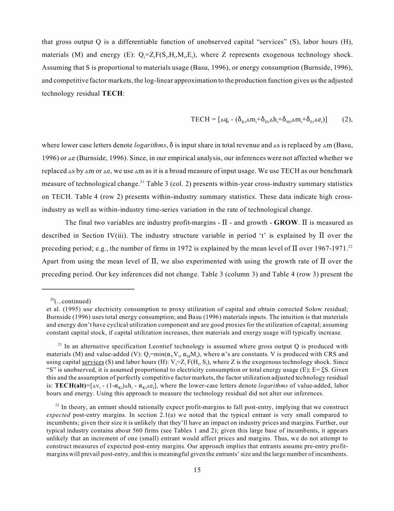
that gross output Q is a differentiable function of unobserved capital “services” (S), labor hours (H),

materials (M) and energy (E): Qt=ZtF(St,Ht,Mt,Et), where Z represents exogenous technology shock.

Assuming that S is proportional to materials usage (Basu, 1996), or energy consumption (Burnside, 1996),

and competitive factor markets, the log-linear approximation to the production function gives us the adjusted

technology residual TECH:

TECH = [ªqt - (*Ktªmt+*Htªht+*M tªmt+*Etªet)] (2),

where lower case letters denote logarithms, * is input share in total revenue and ªs is replaced by ªm (Basu,

1996) or ªe (Burnside, 1996). Since, in our empirical analysis, our inferences were not affected whether we

replaced ªs by ªm or ªe, we use ªm as it is a broad measure of input usage. We use TECH as our benchmark

measure of technological change.21 Table 3 (col. 2) presents within-year cross-industry summary statistics

on TECH. Table 4 (row 2) presents within-industry summary statistics. These data indicate high cross-

industry as well as within-industry time-series variation in the rate of technological change.

The final two variables are industry profit-margins - A - and growth - GROW. A is measured as

described in Section IV(iii). The industry structure variable in period ‘t’ is explained by A over the

preceding period; e.g., the number of firms in 1972 is explained by the mean level of A over 1967-1971.22

Apart from using the mean level of A, we also experimented with using the growth rate of A over the

preceding period. Our key inferences did not change. Table 3 (column 3) and Table 4 (row 3) present the

16

cross-industry and within-industry summary statistics on A. Our proxy for industry growth is the mean rate

of new (net) investment. New investment entails sunk costs; thus if new investment is increasing, it is likely

to indicate expanding market opportunities. As is standard (e.g., Fazzari et al., 1988), we measure net

investment by the ratio (Ii,t/Ki,t-1), where Ii,t is total industry investment in the current period and Ki,t-1 is the

end of last period capital stock. The industry structure variable in period ‘t’ is explained by the mean rate

of net investment over the preceding period; e.g., the number of firms in 1972 is explained by the mean rate

of net investment over 1967-1971. Table 3 (column 3) and Table 4 (row 3) present the cross-industry and

within-industry summary statistics on GROW. As a check of robustness, in Section VI we report estimates

using industry sales growth as a proxy for growth; our results regarding uncertainty are not affected.

V. Panel Data Model

Entry and exit are not likely to occur instantaneously to restore an industry’s equilibrium under changing

conditions, and there is uncertainty regarding the time is takes to restore equilibrium. With these

considerations, we use a partial adjustment model to structure our within-industry time-series equation.

Martin (1993, Ch.7), e.g., reviews studies that have used similar models. Denoting industry structure by

STR, where STR could be FIRMS, ESTB (and by size groups) or CONC, we get:

STRi,t = 8STRi,t* - (1-8)STRi,t-1 (3),

where i and t denote industry and time, STR* the equilibrium structure in period t, and 8 the partial-

adjustment parameter. STR* is not observed and is modeled as a function of the following industry-specific

variables: (i) profit uncertainty, F(A)i,t; (ii) technological change, TECHi,t; (iii) profit-margin, Ai,t; and (iv)

growth, GROWi,t. Apart from (i)-(iv), the panel data model includes the following controls: (v) an industry-

specific fixed-effect "i to control for unobserved factors that influence the long-run level of industry

structure, STR. These include unobserved relatively time-invariant elements of scale economies, advertising

and R&D (see discussion in Section III(ii)); and (vi) an aggregate structure variable, ASTR, to control for

manufacturing-wide effects common to all industries. Audretsch (1995, Ch.3), for example, finds that

macroeconomic factors play an important role; ASTR will capture these aggregate effects.

Incorporating these features, the dynamic panel data model is given by:

STRi,t = "i + >1F(A)i,t + >2TECHi,t + >3Ai,t + >4GROWi,t + >5ASTRt + >6STRi,t-1 + ,i,t (4).

17

The variables STR, F(A), A, GROW and ASTR are measured in logarithms; thus, these coefficients are

interpreted as elasticities. TECH is not measured in logarithms as it can be negative or positive (see Section

IV(iv) for construction of TECH). Next, we clarify the setup of (4). Let STRi,t be FIRMSi ,1972. Then F(A)i ,1972

is standard deviation of residuals over 1967-1971; TECHi ,1972 the mean rate of technical change over 1967-

71; Ai ,1972 the mean profit-margin over 1967-71; GROWi ,1972 the mean rate of net investment over 1967-71;

AFIRMS1972 the total number of firms in manufacturing in 1972; and FIRMSi ,1967 (the lagged dependent

variable) the total number of firms in the 4-digit industry in 1967. As discussed in Section III(ii), the lagged

dependent industry structure variable will capture aspects of scale economies, and advertising and R&D

intensities using information from the recent past. We estimate (4) for all industries in our sample as well

as the sunk cost sub-samples.

Estimation Method

First, as shown in the literature on estimation of dynamic panel data models, we need to instrument the

lagged dependent variable STRi,t-1. Second, industry-specific variables like number of establishments and

firms, profit-margins, output, input usage, technical change (constructed from data on industry output and

inputs) are all likely to be jointly-determined in industry equilibrium and are best treated as endogenous.

Several estimators have been proposed to obtain efficient and unbiased estimates in dynamic panel models;

see, e.g., Kiviet (1995). Our estimation proceeds in two steps. First, we sweep out the industry intercept "i

by taking deviations from within-industry means; the data are now purged of systematic differences across

industries in the level of the relevant structure variable. Second, the within-industry equation is estimated

using the instrumental variable (IV) estimator, treating F(A)i,t, TECHi,t, Ai,t, GROWi,t, and STRi,t-1 as

endogenous. We include a broad set of instruments as the literature indicates this is needed to alleviate

problems related to bias and efficiency. The variables and their instruments are:

(a) F(A)i,t is instrumented by F(A)i,t-1 and F(A)i,t-2. In addition, since our data are over 5-year time intervals

(e.g., F(A)i ,1977 is constructed using data over 1972-1976), we also include instruments constructed at a

higher level of aggregation that are likely to be correlated with F(A)i,t and uncorrelated with the error term.

The objective being to provide a stronger set of instruments. We adopt the following procedure: we segment

our data into durable (D) and non-durable (ND) goods industries. The business cycle literature indicates

that these two types of industries show markedly different fluctuations. It is unlikely that any one D or ND

4-digit industry will systematically influence all the D or ND industries; fluctuations in the entire D or ND

group will be driven by factors exogenous to a given industry. Thus, instruments at the D/ND level appear

reasonable. The instrument for F(A)i,t is the standard deviation of D/ND profit-margins over the relevant

18

period. For example, for F(A)i ,1977 the instrument is the standard deviation of A (for D and ND) over 1972-

1976: we label this as F(A: D/ND)t.

(b) For TECHi,t, Ai,t and GROWi,t, we include their own two lags. As with uncertainty, we also include

instruments constructed at the D/ND level: TECH(1: D/ND)t, A(D/ND)t and GROW(D/ND)t.

(c) STRi,t-1 is instrumented by STRi,t-2 and manufacturing-wide ASTRt and ASTRt-1 since ASTR can be

treated as exogenous to a given 4-digit industry.

Finally, we conducted Hausman tests (see Table 6) which easily rejected the null that the industry variables

are pre-determined. We examined the fit of the panel first-stage regressions of the endogenous variables on

the instruments; the R2's were in the 0.15-0.35 range, which are reasonable for panel regressions.

VI. Estimation Results

Estimates From the Full Sample

Table 6 presents results from estimating equation (4). First, we focus on the F(A) estimates; the coefficients

are interpreted as elasticities since the industry structure variables and F(A) are measured in logarithms.

First, examining the broader picture, during periods of greater F(A) there is a decrease in FIRMS and

increase in CONC. Looking at the underlying distribution of establishments, the coefficients are negative

and significant for all establishments and the small establishment groups; the coefficient is positive and

insignificant for the large establishment group. As establishment size decreases (e.g., Size<500; Size<250;

Size<100; Size<50), the F(A) elasticity gets larger. Regarding quantitative effects, a one-s.d. increase in

F(A) results in a drop of 60 FIRMS over the 5-year Census interval, starting from a mean value of 558

FIRMS; and there is a 5 point increase in the four-firm concentration ratio, starting from a mean value of

39%. For 'small' establishment groups, a one-s.d. increase in F(A) leads to decrease of 75-100 establishments

starting from sample mean values of 600-500. The quantitative effects for the number of firms and

establishments are clearly economically meaningful. While we have data on establishments by size groups,

we only have data on the total number of firms. So we can’t make a direct inference on whether the number

of small or large firms are decreasing. But we can make an indirect inference. First, summary statistics

presented in Section IV(i) indicate rough equivalence between an establishment and a firm with the 50th

(75th) percentile value of the ratio [#establishments/#firms] being 1.1 (1.3). Second, the decline in the

number of small establishments is roughly similar to the drop in number of firms. Thus, it appears

reasonable to conclude there is a reduction in the number of small firms in an industry. Overall, periods of

greater uncertainty lead to a reduction in the number of small firms and establishments, and increases

industry concentration. Given the results on small v. large firms and establishments, we can say that the firm

19

(establishment) size distribution becomes less skewed.

TECH has a negative impact on FIRMS; the coefficient of CONC is positive but statistically

insignificant; reduces the number of small establishments; and the impact on large establishments is positive

but insignificant. (Note that TECH is not measured in logarithms.) The point estimate of TECH gets larger

as establishment size gets smaller. Regarding quantitative effects, a one-s.d. increase in TECH leads to a

decrease of 22 FIRMS over the 5-year Census interval, a 1.6 point increase in CONC, and a decrease of

about 30-40 smaller establishments. Thus, technical change reduces the number of small firms and

establishments, increases industry concentration and makes the firm (establishment) size distribution less

skewed. Our results are quite similar to those in Audretsch (1995) where industry-wide innovation has an

adverse impact on small incumbent firms and new startups. Our estimates also indicate that the quantitative

effect of uncertainty on industry dynamics is greater than that of technological change.

The industry structure variables in general co-vary positively with their aggregate (ASTR)

counterparts; the exceptions being the number of large establishments. This indicates that the number of

smaller firms and establishments are more sensitive to business cycle conditions. This finding is similar in

spirit to those in Audretsch (Ch.3) where new firm startups were more sensitive to macroeconomic growth

as compared to industry-specific growth. Profit-margins, A, appear to have no effect on the number of small

establishments and firms, or in the full sample, but have a positive effect on the number of large

establishments; industry CONC rises. Industry growth, GROW, has a negative and significant effect on the

number of large establishments, and a weak negative effect in the full sample. The general ambiguity of the

profit and growth results appear to be similar to those observed in some of the previous literature (see

Section III(ii)). Finally, apart from CONC, the lagged dependent variables are positive and significant.

Sunk Cost Sub-Samples

The predictions from theory were that presence of higher sunk costs are likely to exacerbate the impact of

uncertainty; we examine this. In Table 7 we only present the F(A) estimates; for ease of comparison, the

first column reproduces the full-sample estimates from Table 6. The following observations emerge:

(a) For FIRMS, the F(A) elasticities are negative and significant only in the high sunk cost sub-samples. The

only close call is for the low SUNK(EC) group where the elasticity is negative and close to significance at

the 10% level. Given the rough equivalence between establishments and firms, and the results in (e) below,

uncertainty reduces the number of small firms in high sunk cost industries.

(b) F(A) elasticities are positive for CONC, but statistically significant only in the high sunk cost samples.

20

(c) For all establishments (Size All), greater F(A) has a statistically significant negative effect only in the

high sunk costs sub-samples. While the elasticities vary somewhat across the alternative sunk cost measures,

the qualitative inferences are similar. The F(A) elasticities are insignificant in the low sunk cost samples;

(d) For large establishments (Size $500), F(A) is statistically insignificant and positive. The exception being

the DEPR high sunk cost sub-sample where the F(A) coefficient is negative and significant.

(e) Greater F(A) reduces the number of small establishments only in the high sunk cost groups. And, as the

size class get smaller (Size<500; ...; Size<50), the F(A) elasticities get larger in the high sunk cost

categories. The exception being the SUNK(EC) groups where greater F(A) reduces the number of small

establishments even when sunk cost are low, but the elasticities are larger in the high sunk cost group.

Table 8 presents results from sunk cost sub-samples created by “combining” alternative measures

(Section IV(ii)). While the results are similar to those in Table 7, the elasticities in Table 8 present a starker

effect of uncertainty on the dynamics of small firms and establishments. As before, uncertainty does not

have an effect on the number of large establishments in an industry irrespective of the degree of sunk costs.

Regarding industry dynamics, the broad picture emerging from Tables 7 and 8 is that periods of greater

uncertainty in conjunction with high sunk costs: (i) reduces the number of small firms and establishments;

(ii) has no impact on the number of large establishments; (iii) results in a less skewed firm/establishment

size distribution; and (iv) leads to an increase in industry concentration.

Some Checks of Robustness

To gauge the robustness of our uncertainty results, we carried out numerous checks. Table 9 reports some

of these results. Since the focus of this paper is on the effect of uncertainty and sunk costs, we only report

the F(A) estimates. Panel A reproduces the estimates from Table 6 for easy reference.

(a) We experimented with alternative specifications for the profit forecasting equation (1). First, following

Ghosal (2000), we replaced the broad business cycle indicator, unemployment rate, by the federal funds rate

(FFR) and energy price growth (ENERGY) and constructed the uncertainty measure using these residuals;

these results are in Panel B. Second, we estimated an AR(2) model; these results are in Panel C.

(b) We constructed an alternative measure of industry profit-margins by accounting for depreciation

expenses. The data on industry-specific depreciation rates were collected for the Census years 1972, 1982

and 1992 (same as those used to create the DEPR sub-samples). We assumed that the mean depreciation rate

(over 72, 82 and 92) was representative for the full sample period and constructed the measure as:

A(alt)=[(Total Sales Revenue-Total Variable Costs-Depreciation Expenses)/(Total Sales Revenue)].

Using this measure, we reestimated equation (1) to construct F[A(alt)]. We did not report these as our main

21

results since we do not have a time-series in depreciation rates which would be required to make a proper

comparison with our main measure F(A). The results using F[A(alt)] are in Panel D.

(c) In the main regression, we used the rate of new investment to proxy industry growth, GROW. We used

an alternative measure, the growth of industry sales, and re-estimated equation (4); results are in Panel E.

While in Table 9 we only report the equivalent of Table 6 estimates, we also examined the equivalent of

Tables 7 and 8 sunk cost sub-sample estimates; we do not present the latter as they would be very space

consuming. The above checks did not alter our broad inferences from Tables 6-8.

(d) We experimented with: (i) estimating equation (4) using GMM instead of the Instrumental Variables

method; (ii) varying the lag length of the explanatory variables in equation (1); (iii) estimating the profit

forecasting equation in growth rates instead of levels; and (iv) an alternative instrument for F(A) by

constructing the (durable/non-durable) D/ND profit uncertainty instrument (Section V) by estimating a

forecasting equation and using the residuals, instead of simply taking the standard deviation of D/ND profits.

We separately estimated equation (1) with annual (1958-94) data on D and ND profit-margins. Uncertainty

was measured using the standard deviation of residuals. There were small quantitative differences, but the

broad inferences from Tables 6-8 were not affected.

VII. Concluding Remarks

Our results suggest that periods of greater uncertainty about profits, in conjunction with higher sunk costs,

have a quantitatively large negative impact on the survival rate of smaller firms, retard entry and lead to a

less skewed firm size distribution; the impact on industry concentration is positive, but quantitatively small.

Our findings shed light on some of the factors influencing the intertemporal dynamics of industry structure

and the evolution of firm size distribution, and lend support to Sutton’s (1997.a, p.53) insight that

fluctuations in industry profits may be of primary importance in understanding industry dynamics. How do

these findings square up with respect to the option value and financing constraints channels discussed in

Section II? For the option value channel, numerical simulations in Dixit and Pindyck indicated that, during

periods of greater uncertainty, the entry trigger price was likely to increase by more than the decrease in the

exit trigger price implying negative net entry; the effect would be exacerbated under higher sunk costs.

Further, we argued that the preponderance of these effects would be felt by the relatively smaller firms. Our

empirical findings appear supportive of this channel. Regarding financing constraints, uncertainty and sunk

costs, which increase the probability of bankruptcy and heighten information asymmetries, were expected

to affect smaller firms (incumbents and likely entrants) more than larger firms. Our empirical results also

appear supportive of this channel. The broad nature of our data make it difficult to assess the relative

22

importance of these two channels. Detailed longitudinal studies, along with data on entry and exit, may help

disentangle the effects and provide deeper insights.

Technological change reduces the number of small firms and establishments, with little effect on

larger establishments. Although we use a very different measure of technical change (adjusted Solow

residual) than employed in the previous literature (R&D, innovations, patents), our findings are similar to

Audretsch (1995) where industry-wide innovation adversely affects startups and smaller incumbents.

Audretsch noted his findings were consistent with the hypothesis of routinized technological regime. Our

findings, however, also appear consistent with the notions outlined in Gort and Klepper (1982) where

efficiency enhancing incremental technical change weeds out inefficient firms and creates barriers to entry.

23

DATA APPENDIX

Data on industry structure and sunk cost measures were collected from various Census reports. The tablebelow summarizes the sources and years for which data are available. Industry time-series data are at theSIC 4-digit level; see Bartlesman, Eric, and Wayne Gray. “The Manufacturing Industry ProductivityDatabase,” National Bureau of Economic Research, 1998. The following industries were excluded from thesample: (i) “Not elsewhere classified” since they do not correspond to well defined product markets; (ii)Industries that could not be matched properly over time due to SIC definitional changes; there wereimportant definition changes in 1972 and 1987. For these industries, the industry time-series and otherstructural characteristics data are not comparable over the sample period; and (iii) Industries that hadmissing data on industry structure and sunk cost variables. The final sample contains 267 SIC 4-digitmanufacturing industries that are relatively well defined over the sample period and have data consistency.

Variable(s) Source Years Available

Number of firms Census of Manufacturing 1963, 67, 72, 77, 82, 87, 92.

Four-firm concentration Census of Manufacturing 1963, 67, 72, 77, 82, 87, 92.

Number of establishments by size Census of Manufacturing 1963, 67, 72, 77, 82, 87, 92.

Used capital expenditures Census of Manufacturing 1972, 82, 92.

Rental payments Census of Manufacturing 1972, 82, 92.

Depreciation payments Census of Manufacturing 1972, 82, 92.

Industry time-series: sales, costs,investment, capital stock, etc.

Bartlesman and Gray (1998). Annual: 1958-1994

Aggregate: energy price, federalfunds and unemployment rate.

Economic Report of thePresident.

Annual: 1958-1994.

24

REFERENCES

Appelbaum, Elie, and Chin Lim. “Contestable Markets under Uncertainty,” RAND Journal of Economics,1985, 28-40.

Audretsch, David. Innovation and Industry Evolution. Cambridge: MIT Press, 1995.

Basu, Susanto. “Procyclical Productivity: Increasing Returns or Cyclical Utilization?” Quarterly Journalof Economics, 1996, 719-751.

Baumol, William, John Panzar, and Robert Willig. Contestable Markets and the Theory of IndustryStructure. San Diego: Harcourt Brace Jovanovich, 1982.

Brito, Paulo and Antonio Mello. “Financial Constraints and Firm Post-Entry Performance,” InternationalJournal of Industrial Organization, 1995, 543-565.

Burnside, Craig. “Production Function Regressions, Returns to Scale, and Externalities,” Journal ofMonetary Economics 37, 1996, 177-201.

Caballero, Ricardo, and Robert Pindyck, “Investment, Uncertainty and Industry Evolution,” InternationalEconomic Review, 1996, 641-662.

Caballero, Ricardo, and Mohamad Hammour. “The Cleansing Effect of Recessions,” American EconomicReview, 1994, 1350-1368.

Cable and Schwalbach (1991): International Comparisons of Entry and Exit,” in P. Geroski and J.Schwalbach (eds.), Entry and Market Contestability: An International Comparison. Basil Blackwell, 257-81.

Cabral, Luis and Jose Mata. “On the Evolution of the Firm Size Distribution: Facts and Theory,” AmericanEconomic Review, 2003, forthcoming.

Caves, Richard. “Industrial organization and New Findings on the Turnover and Mobility of Firms,” Journalof Economic Literature, 1998, 1947-1982.

Cohen, Wesley and Richard Levin. “Empirical Studies of Innovation and Market Structure” in Schmalensee,Richard and Robert Willig, ed., Handbook of Industrial Organization, Amsterdam: North Holland, (1989).

Cooley, Thomas and Vincenzo Quadrini. “Financial Markets and Firm Dynamics,” American EconomicReview, 2001, 1286-1310.

Davis, Steven, John Haltiwanger and Scott Schuh. Job Creation and Destruction. MIT Press, 1996.

Dixit, Avinash. “Entry and Exit Decisions under Uncertainty,” Journal of Political Economy, 1989, 620-38.

Dixit, Avinash, and Robert Pindyck. Investment under Uncertainty. Princeton University Press, 1996.

Domowitz, Ian, Glenn Hubbard and Bruce Petersen. “Business Cycles and the Relationship BetweenConcentration and Price-Cost Margins,” RAND Journal of Economics, 1986, 1-17.

25

Domowitz, Ian, Glenn Hubbard, and Bruce Petersen. “Oligopoly Supergames: Some Evidence on Prices andMargins,” Journal of Industrial Economics, 1987, 379-98.

Dunne, Timothy, Mark Roberts, and Larry Samuelson. “Patterns of Entry and Exit in U.S. manufacturingindustries,” RAND Journal of Economics, 1988, 495-515.

Evans, David. “The Relationship Between Firm Growth, Size and Age: Estimates for 100 ManufacturingIndustries,” Journal of Industrial Economics, 1987, 567-581.

Evans, David and Boyan Jovanovic. “An Estimated Model of Entrepreneurial Choice under LiquidityConstraints,” Journal of Political Economy, 1989, 808-827.

Evans, Laurie, and John Siegfried. “Entry and Exit in U.S. Manufacturing from 1977-82.” In D. Audretschand J. Siegfried (eds.), Empirical Studies in Industrial organization: Essays in Honor of Leonard Weiss.Boston: Kluwer Academic Publishers, 253-274.

Fazzari, Steven, Glenn Hubbard and Bruce Petersen, “Financing Constraints and Corporate Investment.”Brookings Papers on Economic Activity, 1988, 141-195.

Geroski, Paul. “What do we know about Entry?” International Journal of Industrial Organization, 1995,421-440.

Geroski, Paul, and Joachim Schwalbach. Entry and Market Contestability. Oxford: Blackwell, 1991.

Gertler, Mark, and Simon Gilchrist. “Monetary Policy, Business Cycles, and the Behavior of SmallManufacturing Firms,” Quarterly Journal of Economics, 1994, 309-340.

Ghosal, Vivek. “Product Market Competition and Industry Price-Cost Margin Fluctuations: Role of EnergyPrice and Monetary Changes,” International Journal of Industrial Organization, 2000, 415-444.

Ghosal, Vivek and Prakash Loungani. “The Differential Impact of Uncertainty on Investment in Small andLarge Businesses,” The Review of Economics and Statistics, 2000, 338-343.

Ghosal, Vivek and Prakash Loungani. “Product Market Competition and the Impact of Price Uncertaintyon Investment,” Journal of Industrial Economics, 1996, 217-228.

Gort, Michael and Steven Klepper. “Time Paths in the Diffusion of Product Innovations,” EconomicJournal, 1982, 630-653.

Greenwald, Bruce and Joseph Stiglitz. “Macroeconomic Models with Equity and Credit Rationing,” inHubbard, R. Glenn. ed., Asymmetric Information, Corporate Finance, and Investment. Chicago: Universityof Chicago Press, 1990, 15-42.

Griliches, Zvi (ed). R&D, Patents and Productivity. Chicago: University of Chicago Press, 1984.

Hopenhayn, Hugo. “Entry, Exit and Firm Dynamics in Long Run Equilibrium,” Econometrica, 1992, 1127-1150.

26

Ijiri,Yuji, and Herbert Simon. Skew Distributions and Sizes of Business Firms. North Holland, 1977.

Jovanovic, Boyan and Peter Rousseau. “Mergers and Technological Change,” Mimeo, University ofChicago, May 2001.

Jovanovic, Boyan and Glenn MacDonald. “The Life Cycle of a Competitive Industry,” Journal of PoliticalEconomy, 1994, 322-347.

Kessides, Ioannis. “Market Concentration, Contestability and Sunk Costs,” Review of Economics andStatistics, 1990, 614-622.

Kiviet, Jan. “On Bias, Inconsistency, and the Efficiency of Various Estimators in Dynamic Panel DataModels,” Journal of Econometrics, 1995, 53-78.

Lambson, Val. “Industry Evolution with Sunk Costs and Uncertain Market Conditions,” InternationalJournal of Industrial Organization, 1991, 171-196.

Lensink, Robert, Hong Bo, and Elmer Sterken. Investment, Capital Market Imperfections, and Uncertainty.Edward Elgar. 2001.

Machin, Stephen, and John Van Reenen, “Profit Margins and the Business Cycle: Evidence from U.K.Manufacturing Firms,” Journal of Industrial Economics, 1993, 29-50.

Martin, Stephen. Advanced Industrial Economics. Oxford: Blackwell, 1993.

Pakes, Ariel, and Richard Ericson. “Empirical Implications of Alternate Models of Firm Dynamics,” Journalof Economic Theory, 1998, 1-45.

Schmalensee, Richard, “Inter-Industry Studies of Structure and Performance,” in Schmalensee, Richard andRobert Willig, ed., Handbook of Industrial Organization, Amsterdam: North Holland, (1989).

Shleifer, Andrei, and Robert Vishny. “Liquidation Values and Debt Capacity: A Market EquilibriumApproach,”Journal of Finance, 1992, 1343-1366.

Spencer, Barbara, and James Brander. “Pre-Commitment and Flexibility: Applications to OligopolyTheory,” European Economic Review, 1992, 1601-1626.

Stiglitz, Joseph, and Andrew Weiss. “Credit Rationing in Markets with Imperfect Information,” AmericanEconomic Review, 1981, 393-410.

Sutton, John. Sunk Costs and Market Structure. Cambridge: MIT Press, 1991.

Sutton, John. “Gibrat’s Legacy,” Journal of Economic Literature, 1997(a), 40-59.

Sutton, John. Technology and Market Structure. Cambridge: MIT Press, 1997(b).

Williamson, Oliver. “Corporate Finance and Corporate Governance,” Journal of Finance, 1988, 567-591.

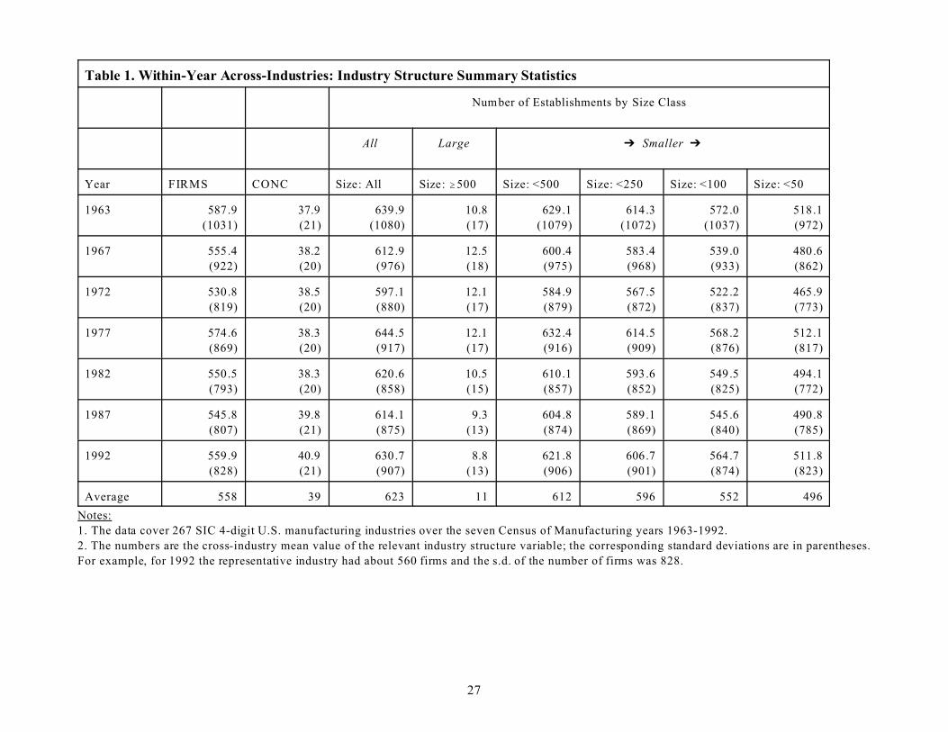
27

Table 1. Within-Year Across-Industries: Industry Structure Summary Statistics

Number of Establishments by Size Class

All Large ö Smaller ö

Year FIRMS CONC Size: All Size: $500 Size: <500 Size: <250 Size: <100 Size: <50

1963 587.9

(1031)

37.9

(21)

639.9

(1080)

10.8

(17)

629.1

(1079)

614.3

(1072)

572.0

(1037)

518.1

(972)

1967 555.4

(922)

38.2

(20)

612.9

(976)

12.5

(18)

600.4

(975)

583.4

(968)

539.0

(933)

480.6

(862)

1972 530.8

(819)

38.5

(20)

597.1

(880)

12.1

(17)

584.9

(879)

567.5

(872)

522.2

(837)

465.9

(773)

1977 574.6

(869)

38.3

(20)

644.5

(917)

12.1

(17)

632.4

(916)

614.5

(909)

568.2

(876)

512.1

(817)

1982 550.5

(793)

38.3

(20)

620.6

(858)

10.5

(15)

610.1

(857)

593.6

(852)

549.5

(825)

494.1

(772)

1987 545.8

(807)

39.8

(21)

614.1

(875)

9.3

(13)

604.8

(874)

589.1

(869)

545.6

(840)

490.8

(785)

1992 559.9

(828)

40.9

(21)

630.7

(907)

8.8

(13)

621.8

(906)

606.7

(901)

564.7

(874)

511.8

(823)

Average 558 39 623 11 612 596 552 496

Notes:

1. The data cover 267 SIC 4-digit U.S. manufacturing industries over the seven Census of Manufacturing years 1963-1992.

2. The numbers are the cross-industry mean value of the relevant industry structure variable; the corresponding standard deviations are in parentheses.

For example, for 1992 the representative industry had about 560 firms and the s.d. of the number of firms was 828.

28

Table 2. Within-Industry Across-Years: Industry Structure Summary Statistics

Mean Std. Deviation

FIRMS Mean 557.8 834.7

Std. Deviation 129.2 234.3

CONC Mean 38.8 20.0

Std. Deviation 5.9 3.6

Size: All Mean 622.8 895.8

Std. Deviation 138.3 233.9

Size: $500 Mean 10.8 15.2

Std. Deviation 3.5 4.5

Size: <500 Mean 611.9 895.2

Std. Deviation 137.7 233.3

Size: <250 Mean 595.6 889.2

Std. Deviation 136.4 232.3

Size: <100 Mean 551.6 858.1

Std. Deviation 130.3 228.2

Size: <50 Mean 496.2 799.1

Std. Deviation 121.4 218.7

Notes:

1. The data cover 267 SIC 4-digit U.S. manufacturing industries over the seven Census years 1963-92.

2. Row labeled “M ean”: For each industry we computed the “within-industry” mean value of the relevant

industry structure variable; we get 267 observations. This row presents the summary statistics for these means.

For example, over the Census years 1963-92, the representative industry had about 558 firms.

3. Row labeled “Std. Deviation”: For each industry we computed the “within-industry” standard deviation (s.d.)

for the relevant industry structure variable. This column presents summary statistics for these s.d.’s. For example,

for the number of firms the representative industry had a s.d. of about 129.

4. E.g., from 2 and 3, the typical industry had a “within-industry” mean number of firms of 558 and s.d. of 129.

29

Table 3. Within-Year Across-Industries: Explanatory Variables Summary Statistics

Period F(A) TECH A GROW

1958-62 0.0175

(0.0140)

0.0081

(0.0226)

0.2425

(0.0881)

0.0223

(0.0122)

1963-66 0.0203

(0.0120)

0.0088

(0.0190)

0.2576

(0.0876)

0.0263

(0.0097)

1967-71 0.0213

(0.0127)

0.0013

(0.0212)

0.2681

(0.0851)

0.0309

(0.0118)

1972-76 0.0289

(0.0184)

0.0073

(0.0265)

0.2731

(0.0809)

0.0377

(0.0136)

1977-81 0.0239

(0.0143)

0.0033

(0.0257)

0.2757

(0.0838)

0.0549

(0.0214)

1982-86 0.0275

(0.0155)

0.0046

(0.0243)

0.2832

(0.0922)

0.0584

(0.0228)

1987-91 0.0262

(0.0190)

0.0055

(0.0241)

0.3086

(0.1005)

0.0672

(0.0270)

Notes: See Section IV for details on the construction of variables. The numbers are the cross-industry mean value of the relevant variable; the

corresponding standard deviations are in parentheses. For example, for F(A) the representative industry had value of 0.0175 and the s.d. of F(A) was 0.014.

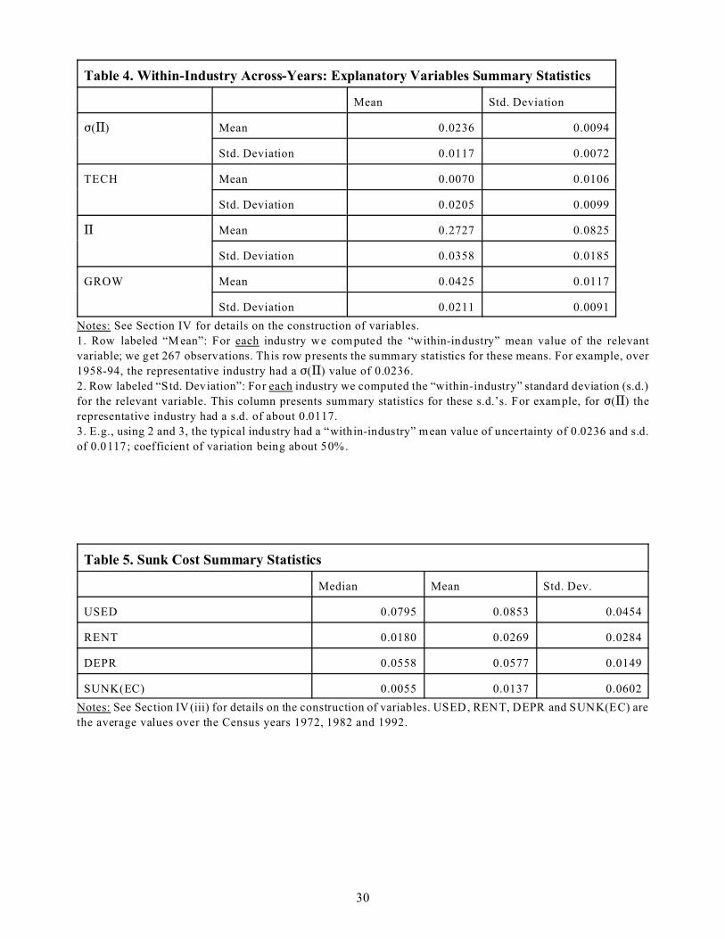
30

Table 4. Within-Industry Across-Years: Explanatory Variables Summary Statistics

Mean Std. Deviation

F(A) Mean 0.0236 0.0094

Std. Deviation 0.0117 0.0072

TECH Mean 0.0070 0.0106

Std. Deviation 0.0205 0.0099

A Mean 0.2727 0.0825

Std. Deviation 0.0358 0.0185

GROW Mean 0.0425 0.0117

Std. Deviation 0.0211 0.0091

Notes: See Section IV for details on the construction of variables.

1. Row labeled “M ean”: For each industry we computed the “within-industry” mean value of the relevant

variable; we get 267 observations. This row presents the summary statistics for these means. For example, over

1958-94, the representative industry had a F(A) value of 0.0236.

2. Row labeled “Std. Deviation”: For each industry we computed the “within-industry” standard deviation (s.d.)

for the relevant variable. This column presents summary statistics for these s.d.’s. For example, for F(A) the

representative industry had a s.d. of about 0.0117.

3. E.g., using 2 and 3, the typical industry had a “within-industry” mean value of uncertainty of 0.0236 and s.d.

of 0.0117; coefficient of variation being about 50%.

Table 5. Sunk Cost Summary Statistics

Median Mean Std. Dev.

USED 0.0795 0.0853 0.0454

RENT 0.0180 0.0269 0.0284

DEPR 0.0558 0.0577 0.0149

SUNK(EC) 0.0055 0.0137 0.0602

Notes: See Section IV(iii) for details on the construction of variables. USED, RENT, DEPR and SUNK(EC) are

the average values over the Census years 1972, 1982 and 1992.

31

Table 6. Estimation Results for All Industries.Equation (4): STRi,t="i+>1F(A)i,t+>2TECHi,t+>3A i,t+>4GROWi,t+>5ASTRt+>6STRi,t-1+,i,t.

Industry Structure Variable: STR

Number of Establishments by Size Class

6 Smaller Size 6

FIRMS CONC Size: All Size: $500 Size: <500 Size: <250 Size: <100 Size: <50

F(A)i, t -0.159**

(0.003)

0.191**

(0.005)

-0.172**

(0.001)

0.093

(0.258)

-0.178**

(0.001)

-0.209**

(0.001)

-0.268**

(0.001)

-0.308**

(0.001)

TECH i, t -1.642*

(0.075)

1.758

(0.193)

-1.737*

(0.057)

0.492

(0.729)

-1.809*

(0.074)

-2.263**

(0.046)

-2.943**

(0.028)

-3.418**

(0.015)

A i, t 0.046

(0.725)

0.507**

(0.028)

0.089

(0.504)

0.421*

(0.029)

0.029

(0.849)

-0.025

(0.879)

0.001

(0.995)

0.042

(0.837)

GROW i, t -0.011

(0.678)

0.058

(0.144)

-0.041*

(0.094)

-0.304**

(0.001)

-0.017

(0.521)

-0.003

(0.916)

0.012

(0.726)

0.004

(0.924)

ASTR t 0.001**

(0.037)

0.074**

(0.003)

0.002**

(0.001)

0.001

(0.778)

0.002**

(0.001)

0.002**

(0.001)

0.003**

(0.002)

0.004**

(0.001)

STR i, t-1 0.267**

(0.001)

-0.049

(0.562)

0.252**

(0.001)

0.261**

(0.001)

0.261**

(0.001)

0.253**

(0.007)

0.233**

(0.005)

0.208**

(0.016)

Panel Obs.

#Industries

Hausman Test

1335

267

92.9 (0.001)

1335

267

67.8 (0.001)

1335

267

126 (0.001)

1335

267

57.2 (0.001)

1335

267

81.3 (0.001)

1335

267

52.3 (0.001)

1335

267

31.8 (0.001)

1335

267

34.6 (0.001)

Notes:

1. Estimation is via the instrumental variables method; instruments are described in Section V. p-values (two-tailed test) computed from heteroscedasticity-

consistent standard errors are in parentheses; ** and * indicate significance at least at the 5% and 10% levels.

2. Hausman test statistics (p-value) easily rejected the null that the industry-specific variables were pre-determined. We also examined fit of the 'first-stage'

panel regressions of the endogenous variables on the instruments: the R2's were in the 0.15-0.35 range, which are reasonably good for panel data.

3. As noted in Section V, the variables STR, F(A), A , GROW and ASTR in equation (4) are measured in logarithms; these coefficients can be interpreted

as elasticities. TECH is not measured in logarithms; thus the magnitude of these coefficients cannot be directly compared to others.

4. Variable definitions (see section IV): FIRMS-number of firms; CONC-four firm concentration ratio; SIZE(.)-number of establishments in a given size

group; F(A)-profit margin uncertainty; TECH-technical change; A-profit margin; GROW -growth; ASTR-corresponding aggregate structure variable.

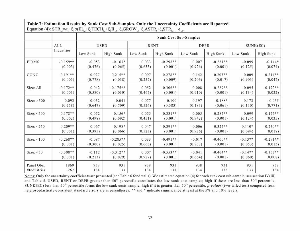
32

Table 7: Estimation Results by Sunk Cost Sub-Samples. Only the Uncertainty Coefficients are Reported.Equation (4): STRi,t="i+>1F(A)i,t+>2TECHi,t+>3A i,t+>4GROWi,t+>5ASTRt+>6STRi,t-1+,i,t.

Sunk Cost Sub-Samples

ALL

Industries

USED RENT DEPR SUNK(EC)

Low Sunk High Sunk Low Sunk High Sunk Low Sunk High Sunk Low Sunk High Sunk

FIRMS -0.159**

(0.003)

-0.053

(0.476)

-0.163*

(0.065)

0.033

(0.635)

-0.298**

(0.001)

0.007

(0.926)

-0.281**

(0.001)

-0.099

(0.125)

-0.144*

(0.074)

CONC 0.191**

(0.005)

0.027

(0.778)

0.215**

(0.038)

0.097

(0.257)

0.278**

(0.009)

0.142

(0.206)

0.203**

(0.017)

0.009

(0.903)

0.214**

(0.047)

Size: All -0.172**

(0.001)

-0.042

(0.580)

-0.175**

(0.030)

0.052

(0.467)

-0.306**

(0.001)

0.008

(0.910)

-0.289**

(0.001)

-0.095

(0.134)

-0.172**

(0.022)

Size: $500 0.093

(0.258)

0.052

(0.647)

0.041

(0.709)

0.077

(0.526)

0.100

(0.383)

0.197

(0.183)

-0.188*

(0.061)

0.173

(0.130)

-0.035

(0.771)

Size: <500 -0.178**

(0.002)

-0.052

(0.498)

-0.156*

(0.092)

0.055

(0.451)

-0.331**

(0.001)

0.005

(0.942)

-0.287**

(0.001)

-0.099

(0.124)

-0.175**

(0.035)

Size: <250 -0.209**

(0.001)

-0.067

(0.395)

-0.198*

(0.066)

0.047

(0.523)

-0.391**

(0.001)

-0.006

(0.936)

-0.327**

(0.001)

-0.110*

(0.094)

-0.230**

(0.018)

Size: <100 -0.268**

(0.001)

-0.087

(0.300)

-0.285**

(0.025)

0.033

(0.663)

-0.491**

(0.001)

-0.017

(0.833)

-0.400**

(0.001)

-0.137*

(0.053)

-0.291**

(0.013)

Size: <50 -0.308**

(0.001)

-0.112

(0.213)

-0.312**

(0.029)

0.007

(0.927)

-0.553**

(0.001)

-0.041

(0.664)

-0.464**

(0.001)

-0.147*

(0.060)

-0.353**

(0.008)

Panel Obs.

#Industries

1869

267

938

134

931

133

938

134

931

133

938

134

931

133

931

133

938

134

Notes: Only the uncertainty coefficients are presented (see Table 6 for details). W e estimated equation (4) for each sunk cost sub-sample; see section IV(iii)

and Table 5. USED, RENT or DEPR greater than 50 th percentile constitutes the low sunk cost samples; high if these are less than 50 th percentile.

SUNK(EC) less than 50th percentile forms the low sunk costs sample; high if it is greater than 50 th percentile. p-values (two-tailed test) computed from

heteroscedasticity-consistent standard errors are in parentheses; ** and * indicate significance at least at the 5% and 10% levels.

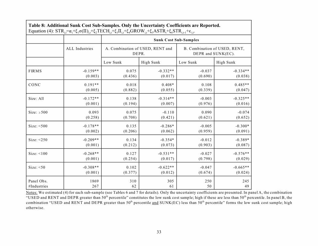
33

Table 8: Additional Sunk Cost Sub-Samples. Only the Uncertainty Coefficients are Reported.Equation (4): STRi,t="i+>1F(A)i,t+>2TECHi,t+>3A i,t+>4GROWi,t+>5ASTRt+>6STRi,t-1+,i,t.

Sunk Cost Sub-Samples

ALL Industries A. Combination of USED, RENT and

DEPR.

B. Combination of USED, RENT,

DEPR and SUNK(EC).

Low Sunk High Sunk Low Sunk High Sunk

FIRMS -0.159**

(0.003)

0.075

(0.436)

-0.332**

(0.017)

-0.037

(0.690)

-0.334**

(0.038)

CONC 0.191**

(0.005)

0.018

(0.882)

0.408*

(0.055)

0.108

(0.339)

0.485**

(0.047)

Size: All -0.172**

(0.001)

0.138

(0.194)

-0.314**

(0.007)

-0.003

(0.976)

-0.325**

(0.016)

Size: $500 0.093

(0.258)

0.075

(0.708)

-0.110

(0.421)

0.090

(0.621)

-0.074

(0.652)

Size: <500 -0.178**

(0.002)

0.135

(0.206)

-0.286*

(0.062)

-0.005

(0.959)

-0.300*

(0.091)

Size: <250 -0.209**

(0.001)

0.134

(0.212)

-0.354*

(0.073)

-0.012

(0.903)

-0.389*

(0.087)

Size: <100 -0.268**

(0.001)

0.127

(0.254)

-0.531**

(0.017)

-0.027

(0.798)

-0.576**

(0.029)

Size: <50 -0.308**

(0.001)

0.102

(0.377)

-0.622**

(0.012)

-0.047

(0.674)

-0.665**

(0.024)

Panel Obs.

#Industries

1869

267

310

62

305

61

250

50

245

49

Notes: We estimated (4) for each sub-sample (see Tables 6 and 7 for details). Only the uncertainty coefficients are presented. In panel A, the combination

“USED and RENT and DEPR greater than 50th percentile” constitutes the low sunk cost sample; high if these are less than 50 th percentile. In panel B, the

combination “USED and RENT and DEPR greater than 50th percentile and SUNK(EC) less than 50 th percentile” forms the low sunk cost sample; high

otherwise.

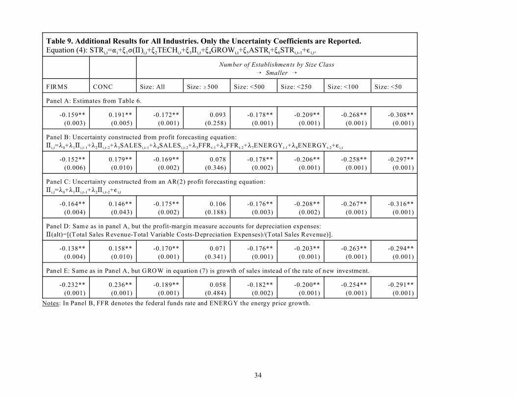
34

Table 9. Additional Results for All Industries. Only the Uncertainty Coefficients are Reported.Equation (4): STRi,t="i+>1F(A)i,t+>2TECHi,t+>3A i,t+>4GROWi,t+>5ASTRt+>6STRi,t-1+,i,t.

Number of Establishments by Size Class

÷ Smaller ÷

FIRMS CONC Size: All Size: $500 Size: <500 Size: <250 Size: <100 Size: <50

Panel A: Estimates from Table 6.

-0.159**

(0.003)

0.191**

(0.005)

-0.172**

(0.001)

0.093

(0.258)

-0.178**

(0.001)

-0.209**

(0.001)

-0.268**

(0.001)

-0.308**

(0.001)

Panel B: Uncertainty constructed from profit forecasting equation:

A i,t=80+81A i,t-1+82A i,t-2+83SALES i,t-1+84SALES i,t-2+85FFR t-1+86FFR t-2+87ENERGYt-1+88ENERGYt-2+, i,t

-0.152**

(0.006)

0.179**

(0.010)

-0.169**

(0.002)

0.078

(0.346)

-0.178**

(0.002)

-0.206**

(0.001)

-0.258**

(0.001)

-0.297**

(0.001)

Panel C: Uncertainty constructed from an AR(2) profit forecasting equation:

A i,t=80+81A i,t-1+82A i,t-2+, i,t

-0.164**

(0.004)

0.146**

(0.043)

-0.175**

(0.002)

0.106

(0.188)

-0.176**

(0.003)

-0.208**

(0.002)

-0.267**

(0.001)

-0.316**

(0.001)

Panel D: Same as in panel A, but the profit-margin measure accounts for depreciation expenses:

A(alt)=[(Total Sales Revenue-Total Variable Costs-Depreciation Expenses)/(Total Sales Revenue)].

-0.138**

(0.004)

0.158**

(0.010)

-0.170**

(0.001)

0.071

(0.341)

-0.176**

(0.001)

-0.203**

(0.001)

-0.263**

(0.001)

-0.294**

(0.001)

Panel E: Same as in Panel A, but GROW in equation (7) is growth of sales instead of the rate of new investment.

-0.232**

(0.001)

0.236**

(0.001)

-0.189**

(0.001)

0.058

(0.484)

-0.182**

(0.002)

-0.200**

(0.001)

-0.254**

(0.001)

-0.291**

(0.001)

Notes: In Panel B, FFR denotes the federal funds rate and ENERGY the energy price growth.

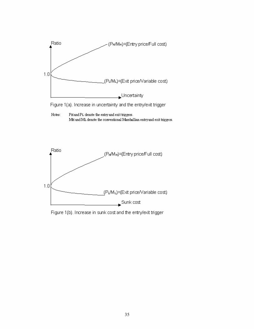
35

36

Notes for Figures 2(a)-2(g): The figures represent the establishment size distribution for the “representatitive” SIC

4-digit industry (i.e., the average across the 267 industries for a given Census year). The establishment size groups

correspond to the following number of employees (in parentheses). G1 (1-4); G2 (5-9); G3 (10-19); G4 (20-49); G5

(50-99); G6 (100-249); G7 (250-499); G8 (500-999); G9 (1,000-2,499); and G10 (2,500 or more). The vertical axis

indicates the share of the number of establishments for that group in the industry total.

Bücher des Forschungsschwerpunkts Markt und politische Ökonomie Books of the Research Area Markets and Political Economy

Andreas Stephan Essays on the Contribution of Public Infrastruc-ture to Private: Production and its Political Economy 2002, dissertation.de

Hans Mewis Essays on Herd Behavior and Strategic Delegation 2001, Shaker Verlag

Andreas Moerke Organisationslernen über Netzwerke – Die personellen Verflechtungen von Führungsgremien japanischer Aktiengesellschaften 2001, Deutscher Universitäts-Verlag

Silke Neubauer Multimarket Contact and Organizational Design 2001, Deutscher Universitäts-Verlag

Lars-Hendrik Röller, Christian Wey (Eds.) Die Soziale Marktwirtschaft in der neuen Weltwirtschaft, WZB Jahrbuch 2001 2001, edition sigma

Michael Tröge Competition in Credit Markets: A Theoretic Analysis 2001, Deutscher Universitäts-Verlag

Tobias Miarka Financial Intermediation and Deregulation: A Critical Analysis of Japanese Bank-Firm-Relationships 2000, Physica-Verlag

Rita Zobel Beschäftigungsveränderungen und organisationales Lernen in japanischen Industriengesellschaften 2000, Humboldt-Universität zu Berlin http://dochost.rz.hu-berlin.de/dissertationen/zobel-rita-2000-06-19

Jos Jansen Essays on Incentives in Regulation and Innovation 2000, Tilburg University

Ralph Siebert Innovation, Research Joint Ventures, and Multiproduct Competition 2000, Humboldt-Universität zu Berlin http://dochost.rz.hu-berlin.de/dissertationen/siebert-ralph-2000-03-23/

Damien J. Neven, Lars-Hendrik Röller (Eds.) The Political Economy of Industrial Policy in Europe and the Member States 2000, edition sigma

Jianping Yang Bankbeziehungen deutscher Unternehmen: Investitionsverhalten und Risikoanalyse 2000, Deutscher Universitäts-Verlag

Christoph Schenk Cooperation between Competitors – Subcontracting and the Influence of Information, Production and Capacity on Market Structure and Competition 1999, Humboldt-Universität zu Berlin http://dochost.rz.hu-berlin.de/dissertationen/schenk-christoph-1999-11-16

Horst Albach, Ulrike Görtzen, Rita Zobel (Eds.) Information Processing as a Competitive Advantage of Japanese Firms 1999, edition sigma

Dieter Köster Wettbewerb in Netzproduktmärkten 1999, Deutscher Universitäts-Verlag

Christian Wey Marktorganisation durch Standardisierung: Ein Beitrag zur Neuen Institutionenökonomik des Marktes 1999, edition sigma

Horst Albach, Meinolf Dierkes, Ariane Berthoin Antal, Kristina Vaillant (Hg.) Organisationslernen – institutionelle und kulturelle Dimensionen WZB-Jahrbuch 1998 1998, edition sigma

Lars Bergman, Chris Doyle, Jordi Gual, Lars Hultkrantz, Damien Neven, Lars-Hendrik Röller, Leonard Waverman Europe’s Network Industries: Conflicting Priorities - Telecommunications Monitoring European Deregulation 1 1998, Centre for Economic Policy Research

Manfred Fleischer The Inefficiency Trap Strategy Failure in the German Machine Tool Industry 1997, edition sigma

Christian Göseke Information Gathering and Dissemination The Contribution of JETRO to Japanese Competitiveness 1997, Deutscher Universitäts-Verlag

DISCUSSION PAPERS 2002

Fredrik Andersson Kai A. Konrad

Human Capital Investment and Globalization in Extortionary States

FS IV 02 – 01

Lars-Hendrik Röller Christian Wey

Merger Control in the New Economy FS IV 02 – 02

Talat Mahmood Klaus Schömann

Die Determinanten der Mirgrationsentscheidung von IT-Hochschulabsolventen aus Pakistan –Empirische Befunde zur Ausgestaltung der deutschen „Green Card“

FS IV 02 – 03

Talat Mahmood Klaus Schömann

The Determinants of the Migration Decision of IT-graduates from Pakistan: Empirical Evidence for the Design of a German "Green Card"

FS IV 02 – 03a

Jos Jansen The Effects of Disclosure Regulation on Innovative Firms: Common Values

FS IV 02 – 04

Jos Jansen The Effects of Disclosure Regulation on Innovative Firms: Private Values

FS IV 02 – 05

Günter Franke Harris Schlesinger

Richard C. Stapleton

Multiplicative Background Risk FS IV 02 – 06

Tomaso Duso On the Politics of the Regulatory Reform: Econometric Evidence from the OECD Countries

FS IV 02 – 07

Johan Lagerlöf Paul Heidhues

On the Desirability of an Efficiency Defense in Merger Control

FS IV 02 – 08

Olivier Cadot Lars-Hendrik Röller

Andreas Stephan

Contribution to Productivity or Pork Barrel? The Two Faces of Infrastructure Investment

FS IV 02 – 09

Justus Haucap Christian Wey

Unionization Structures and Firms’ Incentives for Productivity Enhancing Investments

FS IV 02 – 10

Heidrun C. Hoppe Emre Ozdenoren

Intermediation in Innovation FS IV 02 – 11

Rainer Nitsche On the Effectiveness of Anti-Predation Rules FS IV 02 – 12

Daniel Krähmer Entry and Experimentation in Oligopolistic Markets for Experience Goods

FS IV 02 – 13

J. Peter Murmann The Coevolution of Industries and National Institutions: Theory and Evidence

FS IV 02 – 14

Kai A. Konrad Terrorism and the State FS IV 02 – 15

Robert Nuscheler Physician Reimbursement, Time-Consistency and the Quality of Care

FS IV 02 – 16

Fredrik Andersson Kai A. Konrad

Taxation and Education Investment in the Tertiary Sector

FS IV 02 – 17

Jan Boone ‘Be nice, unless it pays to fight’: A New Theory of Price Determination with Implications for Competition Policy

FS IV 02 – 18

Kai A. Konrad Altruism and Envy in Contests: An Evolutionarily Stable Symbiosis

FS IV 02 – 19

Helmut Bester Kai A. Konrad

Delay in Contests FS IV 02 – 20

Kjell Erik Lommerud Bjørn Sandvik

Odd Rune Straume

Good Jobs, Bad Jobs and Redistribution FS IV 02 – 21

Steffen Huck Vicki Knoblauch Wieland Müller

On the Profitability of Collusion in Location Games FS IV 02 – 22

Ralph Siebert Learning by Doing and Multiproduction Effects over the Life Cycle: Evidence from the Semiconductor Industry

FS IV 02 – 23

Jürgen Bracht Saul Lach

Eyal Winter

Modeling Oligopolistic Price Adjustment in Micro Level Panel Data

FS IV 02 – 24

Steffen Huck Kai A. Konrad

Strategic Trade Policy and the Home Bias in Firm Ownership Structure

FS IV 02 – 25

Daniel Krähmer Delegation versus Authority FS IV 02 – 26

Thomas Knaus Robert Nuscheler

Incomplete Risk Adjustment and Adverse Selection in the German Public Health Insurance System

FS IV 02 – 27

Kurt R. Brekke Robert Nuscheler

Odd Rune Straume

Quality and Location Choices under Price Regulation

FS IV 02 – 28

Kai A. Konrad Inverse Campaigning FS IV 02 – 29

Sebastian Kessing A Note on the Determinants of Labour Share Movements

FS IV 02 – 30

Sebastian Kessing Employment Protection and Product Market Competition

FS IV 02 – 31

Michal Grajek Identification of Network Externalities in Markets for Non-Durables

FS IV 02 – 32

Robert M. Adams Lars-Hendrik Röller

Robin C. Sickles

Market Power in Outputs and Inputs: An Empirical Application to Banking

FS IV 02 – 33

Tomaso Duso Damien J. Neven

Lars-Hendrik Röller

The Political Economy of European Merger Control: Evidence using Stock Market Data

FS IV 02 – 34

Tomaso Duso Astrid Jung

Market Conduct and Endogenous Lobbying: Evi-dence from the U.S. Mobile Telecommunications Industry

FS IV 02 – 35

DISCUSSION PAPERS 2003

Annette Boom Investments in Electricity Generating Capacity under Different Market Structures and with Endogenously Fixed Demand

SP II 2003 – 01

Kai A. Konrad Wolfram F. Richter

Zur Berücksichtigung von Kindern bei umlagefinanzierter Alterssicherung

SP II 2003 – 02

Stergios Skaperdas Restraining the Genuine Homo Economicus: Why the Economy cannot be divorced from its Governance

SP II 2003 – 03

Johan Lagerlöf Insisting on a Non-Negative Price: Oligopoly, Uncertainty, Welfare, and Multiple Equilibria

SP II 2003 – 04

Roman Inderst Christian Wey

Buyer Power and Supplier Incentives SP II 2003 – 05

Sebastian Kessing Robert Nuscheler

Monopoly Pricing with Negative Network Effects: the Case of Vaccines

SP II 2003 – 06

Lars Frisell

The Breakdown of Authority SP II 2003 – 07

Paul Heidhues Nicolas Melissas

Equilibria in a Dynamic Global Game: The Role of Cohort Effects

SP II 2003 – 08

Pablo Beramendi Political Institutions and Income Inequality: The Case of Decentralization

SP II 2003 – 09

Daniel Krähmer Self-Confidence in Contests SP II 2003 – 10

Ralph Siebert The Introduction of New Product Qualities by Incumbent Firms: Market Proliferation versus Cannibalization

SP II 2003 – 11

Vivek Ghosal Impact of Uncertainty and Sunk Costs on Firm Survival and Industry Dynamics

SP II 2003 – 12

Bei Ihren Bestellungen von WZB-Papers schicken Sie bitte unbedingt einen an Sie adressierten Auf-kleber mit sowie je paper eine Briefmarke im Wert von 0,51 Euro oder einen "Coupon Reponse Inter-national " (für Besteller aus dem Ausland)

Please send a self addressed label and postage stamps in the amount of 0.51 Euro or a "Coupon- Reponse International" (if you are ordering from outside Germany) for each WZB-paper requested

Bestellschein Order Form

Absender / Return Address:

Wissenschaftszentrum Berlin für Sozialforschung Presse- und informationsreferat Reichpietschufer 50 D-10785 Berlin-Tiergarten

Hiermit bestelle ich folgende(s) Discussion paper(s):

Please send me the following Discussion paper(s):

Bestell-Nr. / Order no. Autor/in, Kurztitel /Author(s) / Title(s) in brief