VisuaLyzer User Manual User... · 2018-02-04 · Figure 14 Exporting from UCINET..... 22 Figure 15...
119
VisuaLyzer 2.0 User Manual SocioMetrica VisuaLyzer has been developed by Medical Decision Logic, Inc. with support from the National Institute of Drug Abuse (NIDA) through the Small Business Innovation Research (SBIR) Phase II project “A Tool for Network Research on HIV Among Drug Users” (R44 DA012306). Copyright 2005-2007 Medical Decision Logic, Inc. All rights reserved. February 15, 2007
Transcript of VisuaLyzer User Manual User... · 2018-02-04 · Figure 14 Exporting from UCINET..... 22 Figure 15...

VisuaLyzer 2.0 User Manual
SocioMetrica VisuaLyzer has been developed by Medical Decision Logic, Inc.
with support from the National Institute of Drug Abuse (NIDA) through the Small
Business Innovation Research (SBIR) Phase II project “A Tool for Network
Research on HIV Among Drug Users” (R44 DA012306).
Copyright 2005-2007 Medical Decision Logic, Inc. All rights reserved.
February 15, 2007

VisuaLyzer User Manual, v.2.0. Copyright 2005-2007 Medical Decision Logic, Inc. All rights reserved.
2
TABLE OF CONTENTS TABLE OF CONTENTS ..................................................................................................................................... 2 TABLE OF FIGURES .......................................................................................................................................... 5 Medical Decision Logic, Inc. ................................................................................................................................ 7
SocioMetrica VisuaLyzer ..................................................................................................................................... 8 System Requirements ........................................................................................................................................... 8
Disk Space .......................................................................................................................................................... 8 Operating System: ............................................................................................................................................... 8 Screen resolution ................................................................................................................................................. 8
XSB logic programming environment ................................................................................................................ 8
Installation ............................................................................................................................................................. 8 Registration ........................................................................................................................................................... 8
GUIDED TOUR OF VISUALYZER .................................................................................................................. 9 Creating a Graph ................................................................................................................................................. 9 Using Graph Layouts ........................................................................................................................................ 11
Spring-embedding layout .............................................................................................................................. 11
Circular Layout ............................................................................................................................................. 12 Adding Nodes ................................................................................................................................................... 12
Adding Links .................................................................................................................................................... 13 Moving a node .................................................................................................................................................. 14 Display Properties ............................................................................................................................................. 14
Entering Data into VisuaLyzer .......................................................................................................................... 17 Creating Random Data ...................................................................................................................................... 17
Creating Nodes and Links ................................................................................................................................. 17 Node Attributes ................................................................................................................................................. 17
Link Types and Attributes ............................................................................................................................ 19 Multiplex Links ................................................................................................................................................. 20
Importing Data .................................................................................................................................................. 21 UCINET edgelist1/edgearray1 files .............................................................................................................. 21 GraphML files ............................................................................................................................................... 24
DyNetML ...................................................................................................................................................... 26 Microsoft Excel files ..................................................................................................................................... 27 CSV files (comma separated values) ............................................................................................................ 29
Opening a File ................................................................................................................................................... 30 Importing data into an existing file ................................................................................................................... 30
Adding nodes by merging graphs ................................................................................................................. 30 Adding new Node Attributes ........................................................................................................................ 34
Data Export ......................................................................................................................................................... 35 Saving files........................................................................................................................................................ 35 Saving images ................................................................................................................................................... 36
Exporting data ................................................................................................................................................... 36 UCINET Edgelist1 ........................................................................................................................................ 36 UCINET Edgearray1 .................................................................................................................................... 36 GraphML....................................................................................................................................................... 36 DyNetML ...................................................................................................................................................... 36 Microsoft Excel ............................................................................................................................................. 36 Prolog files .................................................................................................................................................... 37

VisuaLyzer User Manual, v.2.0. Copyright 2005-2007 Medical Decision Logic, Inc. All rights reserved.
3
Adjacency Matrix.......................................................................................................................................... 37
Display Options ................................................................................................................................................... 38 Selecting nodes ................................................................................................................................................. 38 Graph Layout .................................................................................................................................................... 39
Moving nodes................................................................................................................................................ 39
Moving links ................................................................................................................................................. 39 Spring Embedding Layout ............................................................................................................................ 40 Circular Layout ............................................................................................................................................. 40 Radial Layout ................................................................................................................................................ 40 Layered Layout ............................................................................................................................................. 40
N-mode Layout ............................................................................................................................................. 44 Best Fit .......................................................................................................................................................... 46 Node Position ................................................................................................................................................ 47
General Options ................................................................................................................................................ 48
Background color .......................................................................................................................................... 49 Background Image ........................................................................................................................................ 50
Node color ..................................................................................................................................................... 50 Group Node Color......................................................................................................................................... 50
Selection Frame Color .................................................................................................................................. 50 Cluster Frame Color ...................................................................................................................................... 50 Position Frame Color .................................................................................................................................... 50
Show Shapes ................................................................................................................................................. 51 Show Images ................................................................................................................................................. 51
Show Labels .................................................................................................................................................. 51 Show Borders ................................................................................................................................................ 51 Show Disabled Nodes ................................................................................................................................... 51
Show ToolTips .............................................................................................................................................. 51
Show Links ................................................................................................................................................... 51 Show Link Arrow ......................................................................................................................................... 51 Show Link Type (relation) ............................................................................................................................ 52
Show Link Label ........................................................................................................................................... 52 Show Link Weight ........................................................................................................................................ 52
AutoOrganize ................................................................................................................................................ 52 Animation ..................................................................................................................................................... 52
Sounds Effects .............................................................................................................................................. 52 Node options ..................................................................................................................................................... 52
Color ............................................................................................................................................................. 54 Shape ............................................................................................................................................................. 54 EImage .......................................................................................................................................................... 56
Size ................................................................................................................................................................ 56 Label Orientation .......................................................................................................................................... 56
Font ............................................................................................................................................................... 56 Disabling Nodes ................................................................................................................................................ 57 Grouping Nodes ................................................................................................................................................ 58 Link options ...................................................................................................................................................... 59
Color ............................................................................................................................................................. 60 Width............................................................................................................................................................. 60 Style .............................................................................................................................................................. 61 Font ............................................................................................................................................................... 61
VisuaLyzer User Manual, v.2.0. Copyright 2005-2007 Medical Decision Logic, Inc. All rights reserved.
4
Arrowhead Color .......................................................................................................................................... 61
Head Length .................................................................................................................................................. 61 Head Width ................................................................................................................................................... 61
Grouping Links ................................................................................................................................................. 61 Attribute-based display options ........................................................................................................................ 62
Node Label .................................................................................................................................................... 64 Node Color .................................................................................................................................................... 65 Node Shape ................................................................................................................................................... 67 Node Size ...................................................................................................................................................... 68 Link Color ..................................................................................................................................................... 69
Legend for attribute-based queries.................................................................................................................... 70 Views ................................................................................................................................................................ 71 Display Relations/Types ................................................................................................................................... 72 Graph Animation .............................................................................................................................................. 74
Data or Network Querying ................................................................................................................................ 76 Node search ....................................................................................................................................................... 76
Linked Pairs comparison................................................................................................................................... 77 Query History.................................................................................................................................................... 79
ANALYZING SOCIAL NETWORK DATA ................................................................................................... 80 Network Level Properties ................................................................................................................................. 80 Node Properties (e.g., Node Centrality)............................................................................................................ 82
Nearest neighbor: .............................................................................................................................................. 86 Shortest Paths .................................................................................................................................................... 87
Cliques and Clusters (Network Sub-Structures/Sub-Groups)........................................................................... 88 Clique Identification ..................................................................................................................................... 88
Clusters and Communities: ............................................................................................................................... 89
Finding clusters ............................................................................................................................................. 90
Finding Communities: .................................................................................................................................. 91 Roles and Positions ........................................................................................................................................... 93 Cutpoints ........................................................................................................................................................... 95
Opinion Leaders ................................................................................................................................................ 97 Algorithm Implementation............................................................................................................................ 98
Core and Periphery ......................................................................................................................................... 100
FORMAL REASONING ABOUT SOCIAL NETWORK DATA ............................................................... 104 Links as Facts .................................................................................................................................................. 104
Boolean operations...................................................................................................................................... 104 Relation operations ..................................................................................................................................... 105 Variables ..................................................................................................................................................... 108
Solving for Unknowns in Deterministic Networks ......................................................................................... 109
Illustrative Examples ...................................................................................................................................... 112 Exploring large hierarchies ............................................................................................................................. 115
Limitations and further information ................................................................................................................ 116 Further Information ......................................................................................................................................... 117
Appendix: Mouse and Keyboard Commands ............................................................................................... 118

VisuaLyzer User Manual, v.2.0. Copyright 2005-2007 Medical Decision Logic, Inc. All rights reserved.
5
TABLE OF FIGURES Figure 1 First screen................................................................................................................................................ 9 Figure 2 Creating a random graph ........................................................................................................................ 10 Figure 3 A random graph ...................................................................................................................................... 10
Figure 4 Spring embedded layout ......................................................................................................................... 11 Figure 5 Circular layout ........................................................................................................................................ 12 Figure 6 Adding a node......................................................................................................................................... 13 Figure 7 Adding a new link .................................................................................................................................. 14 Figure 8 Changing display properties ................................................................................................................... 15
Figure 9 Changed display properties .................................................................................................................... 16 Figure 10 Addition of a new node attribute .......................................................................................................... 18 Figure 11 Toggle node attributes windows ........................................................................................................... 19
Figure 12 Edit link screen ..................................................................................................................................... 20 Figure 13 Multiple links between nodes ............................................................................................................... 21 Figure 14 Exporting from UCINET ...................................................................................................................... 22 Figure 15 Importing from UCINET ...................................................................................................................... 24
Figure 16 Importing from Excel ........................................................................................................................... 27 Figure 17 Importing adjacency matrix from Excel ............................................................................................... 28
Figure 18 Importing from CSV files ..................................................................................................................... 29 Figure 19 Opening saved VisuaLyser files ........................................................................................................... 30 Figure 20 Tree with edge attributes ...................................................................................................................... 31
Figure 21 Addition of nodes to existing graph ..................................................................................................... 32 Figure 22 Square grid 5X5.graphml ..................................................................................................................... 33
Figure 23 3D Cube.graphml ................................................................................................................................. 33 Figure 24 Addition of existing nodes only adds new links ................................................................................... 34
Figure 25 Saving data ........................................................................................................................................... 35 Figure 26 Adjacency matrix screen ...................................................................................................................... 37
Figure 27 Adjacency matrix for movie-by-actor affiliation network ................................................................... 38 Figure 28 Moving links ......................................................................................................................................... 39 Figure 29 Layered Layout setup screen ................................................................................................................ 40
Figure 30 Layered Layout graph ........................................................................................................................... 41 Figure 31 Layered Layout graph 2 ........................................................................................................................ 42 Figure 32 Layered Layout setup screen 2 ............................................................................................................. 43
Figure 33 Layered layout graph 3 ......................................................................................................................... 43 Figure 34 N-mode Network Layout options ........................................................................................................ 44 Figure 35 Simple bipartite graph .......................................................................................................................... 45 Figure 36 Cube graph............................................................................................................................................ 46 Figure 37 Best fit for cube graph .......................................................................................................................... 47
Figure 38 Selected nodes position aligned............................................................................................................ 48 Figure 39 Display properties screen ..................................................................................................................... 49
Figure 40 Display properties Nodes/Links ........................................................................................................... 53 Figure 41 Node properties on display screen ........................................................................................................ 54 Figure 42 Select shape screen ............................................................................................................................... 55 Figure 43 Node labels used as node shapes .......................................................................................................... 55 Figure 44 Font selection screen ............................................................................................................................ 56 Figure 45 Enable nodes screen ............................................................................................................................. 57 Figure 46 Edit group screen .................................................................................................................................. 58

VisuaLyzer User Manual, v.2.0. Copyright 2005-2007 Medical Decision Logic, Inc. All rights reserved.
6
Figure 47 Edit group screen - members ................................................................................................................ 59
Figure 48 Display properties screen - links .......................................................................................................... 60 Figure 49 Edit attributes for group of links .......................................................................................................... 62 Figure 50 Basic graph ........................................................................................................................................... 63 Figure 51 Adding meaning to a basic graph ......................................................................................................... 64
Figure 52 Attribute base selection screen ............................................................................................................. 65 Figure 53 Attribute based selection screen - color tab .......................................................................................... 66 Figure 54 Selecting group of values - color tab .................................................................................................... 67 Figure 55 Attribute based selection screen - shape tab ......................................................................................... 68 Figure 56 Attribute selection screen - size tab ...................................................................................................... 69
Figure 57 Attribute based selection screen - link color tab .................................................................................. 70 Figure 58 Legend window .................................................................................................................................... 71 Figure 59 Loading and saving views .................................................................................................................... 72 Figure 60 Select relation/links .............................................................................................................................. 73
Figure 61 Select type of node ............................................................................................................................... 74 Figure 62 Network animator ................................................................................................................................. 75
Figure 63 Node search .......................................................................................................................................... 76 Figure 64 Result of node search ............................................................................................................................ 77
Figure 65 Linked pairs comparison ...................................................................................................................... 78 Figure 66 Results of linked pairs comparison....................................................................................................... 79 Figure 67 Network Properties ............................................................................................................................... 80
Figure 68 Node properties (degree centrality) ...................................................................................................... 82 Figure 69 Node properties (closeness) .................................................................................................................. 84
Figure 70 Node properties (betweenness)............................................................................................................. 85 Figure 71 Nearest neighbors ................................................................................................................................. 86 Figure 72 Shortest path ......................................................................................................................................... 87
Figure 73 Cliques .................................................................................................................................................. 89
Figure 74 Clusters ................................................................................................................................................. 90 Figure 75 Communities......................................................................................................................................... 91 Figure 76 Roles and positions ............................................................................................................................... 94
Figure 77 Cutpoints............................................................................................................................................... 96 Figure 78 Selecting number of leaders ................................................................................................................. 97
Figure 79 Opinion leaders (selected nodes) .......................................................................................................... 98 Figure 80 Core/Periphery analysis ...................................................................................................................... 102
Figure 81 Determine who reports to, but does not seek the advice of, which manager. .................................... 108 Figure 82 An infection network for a contagious, curable disease ..................................................................... 110 Figure 83 Finding the unknowns (NA) within a deterministic subnetwork ....................................................... 111 Figure 84 Solutions (in red) for missing victims (NA) of b ............................................................................... 112 Figure 85 Links to Position leaders are in black. Opinion leaders are in red. ................................................... 113
Figure 86 The network middle is in black although there is no core. ................................................................. 114 Figure 87 A portion of the NCI ontological hierarchy ....................................................................................... 115

VisuaLyzer User Manual, v.2.0. Copyright 2005-2007 Medical Decision Logic, Inc. All rights reserved.
7
Medical Decision Logic, Inc.
www.mdlogix.com
Founded in 1997, Medical Decision Logic® (MDLogix) is a growing information technology company that
develops software for public and clinical health markets. We create software architectures, components, and
systems to optimize information processes in health research and practice.
Our mission is to use information technology:
To apply public health science, knowledge, and methods in administrative, clinical, community, and
occupational setting; and
To link patients, clinicians, researchers, administrators, and others to enhance health and productivity.
Our goal is to serve customers and researchers by providing:
Effective systems for risk detection and preventive interventions;
Cutting-edge logic technology for diagnosis and decision models;
Products designed to increase efficiency and quality in clinical settings;
Automated generation of billing codes and required documentation

VisuaLyzer User Manual, v.2.0. Copyright 2005-2007 Medical Decision Logic, Inc. All rights reserved.
8
SocioMetrica VisuaLyzer
SocioMetrica VisuaLyzer 2.0 (subsequently referred to as VisuaLyzer) is designed to graphically display small
and mid-sized social networks. Researchers can import their data from UCINET edgelist or edgearray,
GraphML and other formats into graphic network of nodes and the links connecting them. Once displayed, the
visual properties such as color, shape, size, and location of the nodes and links can be customized to create an
informative graphic representation of the data.
VisuaLyzer also provides researchers with a number of network analysis functions. Along with some basic
network parameter estimation, researchers can also calculate cliques, partitions, communities, shortest paths,
nearest neighbors, and roles and positions. Researchers can also submit queries to locate nodes and links that
fulfill specific criteria. For additional analysis researchers can export their data to UCINET, EXCEL, GraphML
and other formats.
VisuaLyzer has been developed by Medical Decision Logic, Inc. with support from the National
Institute of Drug Abuse (NIDA) through the Small Business Innovation Research (SBIR) Phase II
project “A Tool for Network Research on HIV Among Drug Users” (R44 DA012306).
System Requirements
Disk Space
Approximately 18 MB of disk space is required to install VisuaLyzer, including XSB programs.
Operating System:
VisuaLyzer is designed to work with Windows 2000 and Windows XP; its behavior on other operating systems
may be slightly different.
Screen resolution
Screen resolution should not be less than 1024 x 768 pixels. While not required, we recommend using a screen
resolution of 1280 x 1024 or higher.
XSB logic programming environment
In order to perform some of the logical path analyses XSB has to be installed on your local machine. The XSB
package is included in the VisuaLyzer setup program. No additional installation is necessary.
Installation
After downloading, running the file VisuaLyzer2.0setup.exe will install VisuaLyzer on your system.
Registration Optional registration will insure notification of future developments.
VisuaLyzer User Manual, v.2.0. Copyright 2005-2007 Medical Decision Logic, Inc. All rights reserved.
9
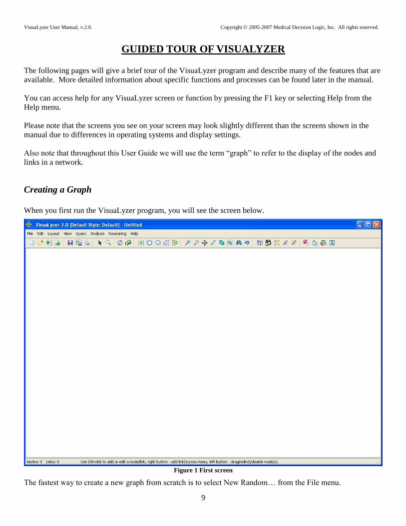
GUIDED TOUR OF VISUALYZER
The following pages will give a brief tour of the VisuaLyzer program and describe many of the features that are
available. More detailed information about specific functions and processes can be found later in the manual.
You can access help for any VisuaLyzer screen or function by pressing the F1 key or selecting Help from the
Help menu.
Please note that the screens you see on your screen may look slightly different than the screens shown in the
manual due to differences in operating systems and display settings.
Also note that throughout this User Guide we will use the term “graph” to refer to the display of the nodes and
links in a network.
Creating a Graph
When you first run the VisuaLyzer program, you will see the screen below.
Figure 1 First screen
The fastest way to create a new graph from scratch is to select New Random… from the File menu.

VisuaLyzer User Manual, v.2.0. Copyright 2005-2007 Medical Decision Logic, Inc. All rights reserved.
10
After selecting New Random… from the File menu you will see the dialog box below.
Figure 2 Creating a random graph
Enter the number of nodes and either the number or percentage of links, click the OK button to see your new
graph. The graph shown below was created with 24 nodes and 138 links.
Figure 3 A random graph
1. Select “New Random…”
from the “File” Menu.
Select the
number of nodes
for your
network here
Enter a number
of links or a
percent of total
possible links here
Click the OK
button
Click spring
embedding layout
button

VisuaLyzer User Manual, v.2.0. Copyright 2005-2007 Medical Decision Logic, Inc. All rights reserved.
11
Using Graph Layouts
You have just created your first graph in VisuaLyzer. However, the randomness of the arrangement of the
nodes makes it difficult to get a good overall view of the network structure, so next we will use automated
layout routines to arrange the graph.
Spring-embedding layout
To organize your graph using a spring-embedding layout, select Spring Embedding Layout from the Layout
menu, press the F9 key, or click the Spring Embedded Layout button below the main menu (Fig.3). This will
re-organize the graph (Fig. 4), which was created with 14 nodes and 16 links.
Figure 4 Spring embedded layout
Note that the disconnected node Node_006 is shown in the upper left corner of the screen. All disconnected
nodes are by default displayed in the upper left corner of the screen so that they can readily be found and moved
into the network if desired.
The spring embedding process may take a minute or more for dense or large graphs but can be stopped by
clicking the Spring Embedded Layout button or pressing the F9 key again.
4. Click the button.
Click the circular layout
icon
VisuaLyzer User Manual, v.2.0. Copyright 2005-2007 Medical Decision Logic, Inc. All rights reserved.
12
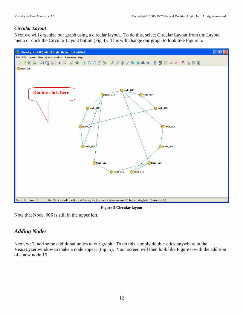
Circular Layout
Next we will organize our graph using a circular layout. To do this, select Circular Layout from the Layout
menu or click the Circular Layout button (Fig 4). This will change our graph to look like Figure 5.
Figure 5 Circular layout
Note that Node_006 is still in the upper left.
Adding Nodes
Next, we‟ll add some additional nodes to our graph. To do this, simply double-click anywhere in the
VisuaLyzer window to make a node appear (Fig. 5). Your screen will then look like Figure 6 with the addition
of a new node 15.
Double-click here

VisuaLyzer User Manual, v.2.0. Copyright 2005-2007 Medical Decision Logic, Inc. All rights reserved.
13
Figure 6 Adding a node
The new node, Node_015, is created and also selected. A node is selected if it is framed as is node 015.
Adding Links
To link two nodes together, right-click and hold on the first node then drag the line (and cursor) to another node
and release the right-click button (Fig. 6). To link an existing node and create a new one at the same time
release the right button at the desired position of the new node. Links can also be created by selecting two
nodes and pressing the F7 key. Figure 7 shows the creation of a new link between the new Node_015 and
Node_001.
Right-click here…
…and drag to here
ere.

VisuaLyzer User Manual, v.2.0. Copyright 2005-2007 Medical Decision Logic, Inc. All rights reserved.
14
Figure 7 Adding a new link
The new link is created and selected, and the two nodes it connects are also selected.
Moving a node
To move a node, click on the node and drag it to a new position on the screen. Nodes can also be “frozen” or
aligned. These issues will be discussed later. The current X and Y coordinates of a selected node will be
displayed in the VisuaLyzer status bar at the bottom of the screen.
Display Properties
VisuaLyzer provides several options for changing the way your graph looks. To view some of these, open the
Display Properties window (Fig. 8), you can:
press F4,
or select View/Edit from the Display listing in the Edit menu,
or click the display properties button (Fig. 7).
Click the display
properties button

VisuaLyzer User Manual, v.2.0. Copyright 2005-2007 Medical Decision Logic, Inc. All rights reserved.
15
Figure 8 Changing display properties
This window was displayed with the Nodes/Links tab showing because Node_015 and Node_001 were
highlighted when we opened it. This tab lets you change the ways nodes and links are displayed. For example,
we can change the size of the nodes by changing the number in the Size field. Change this number from 14 to
28. The size of the nodes will be double that of the others. Note that the Display Properties window will always
stay on top of the graph.
The General tab lets you change display properties for the whole graph. For example, you can display link
weights by clicking the Show Link Weight checkbox, or turn on/off animation of nodes.
a. Change 14 to 28
b. Click the General tab

VisuaLyzer User Manual, v.2.0. Copyright 2005-2007 Medical Decision Logic, Inc. All rights reserved.
16
Figure 9 Changed display properties
Node_015 and Node_001 have been doubled in size and link weights are displayed.

VisuaLyzer User Manual, v.2.0. Copyright 2005-2007 Medical Decision Logic, Inc. All rights reserved.
17
Entering Data into VisuaLyzer
There are several ways to enter or import data into VisuaLyzer. You can create links and nodes directly, have
the VisuaLyzer create random data for you, or import data from several popular formats. Each of these is
described below.
Creating Random Data
VisuaLyzer allows you to create a pseudo-random network graph based on parameters you specify. To create a
new random graph, select New Random… from the File menu. A dialog box will appear (see Fig. 2 above).
Specify the number of nodes you want in your graph in the Number of Nodes field. Then specify either the
number of links you want in your graph in the Number of Links field or the % field. When one of these link
fields is changed, the other will automatically adjust itself. When you have your node and link parameters set,
click the OK button to see your graph. An example of a random graph is shown on page 10 (Fig. 3).
Creating Nodes and Links
VisuaLyzer also allows you to create nodes and links on the screen interactively. To create a node, simply
double-click anywhere on the screen. To create a link between two nodes, right-click on the first node, hold the
right mouse button down, drag the link to the second node, and then release the mouse button (see Fig. 6
above). The direction of the link will be from the first node to the second node. You can also link a node to
itself.
Node Attributes
VisuaLyzer allows you to change the names of your nodes and to add attributes to nodes. To edit a node‟s
information, right-click on the node and then select Edit Node from the pop-up menu. This will bring up the
Edit Node screen (Fig. 10). Double-clicking on a node will also bring up the Edit Node screen. To change the
name of the node, type the new name in the Name field at the top of this screen. The node type can also be
changed, and is set to “actor” by default. To create a new attribute for a node, click the New button. A new
row will be created in the attribute table on the screen. Type the name of the new attribute in the Name cell and
type the value of the attribute in the Value cell. For example, in Figure 9 node 006‟s age is 32.
When a node attribute is created, it is assigned to every node in the graph, but with a value of “na”, or “not
available” ‟ until the user changes it. You can edit an attribute‟s Name or Value by clicking on the cell and
typing in the new information. You can delete a node attribute by selecting that attribute‟s row and then
clicking the Delete button. When you delete a node attribute, you are given two choices:
you can either delete the attribute from all nodes in the graph
or change the value of the existing node‟s attribute to „na‟ and not delete the attribute and values from
all the other nodes in the graph (“soft delete”).

VisuaLyzer User Manual, v.2.0. Copyright 2005-2007 Medical Decision Logic, Inc. All rights reserved.
18
Figure 10 Addition of a new node attribute
You can link the node with a web page or document, for instance, person's resume, photo image, or spreadsheet
data. Just type the path to the destination in the value field, like in the following examples:
http://www.mycompanywebsite.com/docs/myresume.html
C:\photos\mycompany\me.jpg
Clicking the Open button will open the page or document, using the default viewer program.
A node attributes and values will be displayed as a yellow tool tip when the cursor is held over it. These
attributes can also be permanently displayed for selected nodes by clicking the Toggle Attribute Windows
toolbar button, or hitting F3 (Fig. 11).

VisuaLyzer User Manual, v.2.0. Copyright 2005-2007 Medical Decision Logic, Inc. All rights reserved.
19
Figure 11 Toggle node attributes windows
Link Types and Attributes
Links can also have attributes similar to nodes. To enter and edit link information, right-click on a link and
select Edit Link from the pop-up menu. This will bring up the Edit Link screen (Fig. 12). Double-clicking on a
link will also bring up this screen.
Toggle node attributes
windows on or off.

VisuaLyzer User Manual, v.2.0. Copyright 2005-2007 Medical Decision Logic, Inc. All rights reserved.
20
Figure 12 Edit link screen
This screen displays the information about the selected link. Link attributes function just like node attributes for
adding, editing, and deleting them. On this screen you can also change the link‟s Label and Weight by
changing the information in those fields. You can indicate if a link is directed or not directed by selecting the
corresponding Directed radio button. You can change the To Node and From Node of a link by selecting these
nodes in the corresponding drop-down list box.
To assign a web page or document to a link, type the path to the destination in the value field. Clicking the
Open button will open the page or document, using the default viewer program (Fig. 12).
Multiplex Links
VisuaLyzer also allows multiple link types, or relations. This means that one node can be connected to another
node multiple times, with each link being of a different type. If you create a link between two nodes that are
already connected, the above Edit Link screen will be displayed. If you want your new link to be of a different
type, click the label New under the Relation label at the top of this screen, then type in the name of the new
relation and click OK button. This process can be repeated several times as required. Figure 13 shows four

VisuaLyzer User Manual, v.2.0. Copyright 2005-2007 Medical Decision Logic, Inc. All rights reserved.
21
Figure 13 Multiple links between nodes
links between Node_001 and Node_002. Each of these links can have their own properties and attributes. Once
multiple link types have been created between two nodes, each is selectable in the Relation drop-down list box
on the Edit Link screen when one of the links between those two nodes is selected.
Importing Data
VisuaLyzer accepts data input from a variety of file types and formats to allow you to easily use the VisuaLyzer
functions with your existing data. Each of these data types is described below.
UCINET edgelist1/edgearray1 files
Both EdgeList1 and EdgeArray1 files can be exported from UCINET. The edgelist1 format belongs to a
family of linked lists format where a user specifies only ties that actually occur between dyads, and omits those
that did not occur from the data. The edgelist1 format is typically used for square, 1-mode adjacency matrices.
It usually takes the form:
{ego} {alter} {relationship value}
That is, it consists of a list of edges or links (columns 1 and 2), followed by their values (column 3), as shown
in the example below:
dl n = 3 format = edgelist1
labels:
Paul, Liz, Jane
data:
1 2 1
1 3 0
2 1 1
2 3 1
3 1 1
3 2 1
Paul Liz Jane
Paul 0 1 0
Liz 1 0 1
Jane 1 2 0

VisuaLyzer User Manual, v.2.0. Copyright 2005-2007 Medical Decision Logic, Inc. All rights reserved.
22
If the data represents friendship nominations, then the first line indicates that node 1 (Paul) nominates node 2
(Liz) as a friend. This above input data will generate the corresponding adjacency matrix in VizuaLyzer. Note:
both binary and valued relations can be represented using the edgelist1 format. A single edgelist1 file can
represent multiple relations, each of which are separated by a vertical bar or exclamation sign (!).
Acquiring edgelist1 data from UCINET is a two step process: exporting the files from UCINET and importing
them into Visualyzer.
Exporting from UCINET:
1. Select Data > Export DL in UCINET. This will open up the data export window as shown below:
Figure 14 Exporting from UCINET
2. Select input dataset and most importantly, chose edgelist format from the output format drop down box.
3. The data type drop-down box lets you select whether the data is directed (asymmetric) or undirected
(symmetric).
4. Give the output file a meaningful name under output dataset option. Remember edgelists1 files are text
files, and therefore must have the *.txt extension.
5. Click the OK button to save the file. Note the location of the file, so you can copy it into your VisuaLyzer
data directory.
6. The header and fragments of the exported edgelist file looks like this:

VisuaLyzer User Manual, v.2.0. Copyright 2005-2007 Medical Decision Logic, Inc. All rights reserved.
23
7. The header entries provide information about the dataset:
a. DL – indicates it is a DL or UCINET file format;
b. N=21 indicates that there are total of 21 nodes in the matrix;
c. FORMAT = EDGELIST1 DIAGONAL ABSENT indicates that the DL file is exported using the
edgelist1 format, with diagonal entries of the graphs suppressed/absent.
d. DATA: marks the beginning of the actual data
e. ! (Exclamation or vertical mark) at the end of the file indicates the end of one relational matrix,
separating it from other relational matrices (in the case of multi-relational datasets).
8. This procedure will export either a single multiple relation data. Exporting multi-relational datasets
follows the same procedure except that the resulting edgelist1 text file has to be edited slightly to
accommodate differences between UCINET and VisuaLyzer‟s current data specifications:
a. UCINET identifies each relationship in a multi-relational edgelist1 dataset with a label, and
embeds the labels within the data – what it calls “level labels”. This is useful to distinguish
batches of relational data. However, importing such a file gives a known error: "Number of data
sections non-consistent with level labels". To get around this, the user has to remove embedded
level labels in the file - this involves removing the main heading, "LEVEL LABELS
EMBEDDED" as well as the individual labels for each matrix. The multi-relational import
proceeds well after this, though users are advised to keep track of the names and order of the
matrices in the edgelist file. Future versions of VisuaLyzer will support the embedded labels
feature.
DL
N=21
FORMAT = EDGELIST1 DIAGONAL ABSENT
DATA:
1 2 1
1 4 1
1 8 1
1 16 1
1 18 1
1 21 1
2 6 1
2 7 1
2 21 1
21 2 1
21 3 1
21 4 1
21 6 1
21 7 1
21 8 1
21 12 1
21 14 1
21 17 1
21 18 1
21 20 1
!

VisuaLyzer User Manual, v.2.0. Copyright 2005-2007 Medical Decision Logic, Inc. All rights reserved.
24
Importing into VisuaLyzer:
To import files of this type, select Import… from the File menu. This will display a standard Windows file
dialog like the one shown below.
Figure 15 Importing from UCINET
Select UCINET edgelist1/edgearray1 files in the Files of type: box to have these files displayed. When you
have found the file you want to import, either double-click or single-click on it for it to be displayed in the File
name: box and then click the Open button. Your data will be loaded and displayed as a network graph. If the
graph contains any self-loops, VisuaLyzer will prompt you to ignore the self-loops or to keep them.
Note, that to import networks with different link types you can use File > Add function several times. Or you
can use File > Import to import the first network, and then File > Add for the others.
GraphML files
GraphML is a comprehensive and easy-to-use file format for graphs – a variant of XML adapted to describe
graphs. It has predefined words to mark graph's properties, such as "node", "edge", "source", "target",
"directed" etc, and its files can be read it by any XML compatible web browser (e.g., IE), Notepad and can be
processed by XML parsers. The format is convenient for exchanging data with other visualization tools or
MDL software such as QBuilder. Further information about GraphML, its history and background can be found
at: http://graphml.graphdrawing.org/

VisuaLyzer User Manual, v.2.0. Copyright 2005-2007 Medical Decision Logic, Inc. All rights reserved.
25
The GraphML format invariably consists of language core to describe the structural properties of a graph and
optional extension components. An example of the main language core, and the resulting graph is produced
below
Importing a GraphML file:
A GraphML file can be prepared with any text editor or specialized xml editors, according to the format
described above.
The file must be saved with a graphml (*.graphml) extention.
Ensure there are no characters or spaces before the first two lines (or Xml declaration lines) to ensure
format recognition. Examples of the respective lines are (e.g., <?xml version="1.1" encoding="UTF-
8"?> and <!-- This file was written by mdlogix Visualizer 1.1 application. --> ).
To import a GraphML file, select Import… from the File menu. This will display a standard Windows
file dialog like the one in Figure 14, page 22.
Select GraphML files in the Files of type: box to have these files displayed. When you have found the file you
want to import, either double-click or single-click on it for it to be displayed in the File name: box and then
click the Open button. Your data will be displayed as a network graph.
Example 1: Simple graph, no attributes at all, just nodes and edges.
<?xml version="1.1" encoding="UTF-8"?>
<!-- This file was written by mdlogix Visualizer 1.1 application. -->
<!DOCTYPE graphml SYSTEM "http://www.graphdrawing.org/dtds/graphml.dtd">
<graphml>
<graph id="Untitled" edgedefault="directed">
<node id="Allen Tien"/>
<node id="Manyuan"/>
<node id="Steven"/>
<edge source="Allen Tien" target="Manyuan" directed="false"/>
<edge source="Allen Tien" target="Steven" directed="true"/>
</graph>
</graphml>
Manyuan
Allen
Steven

VisuaLyzer User Manual, v.2.0. Copyright 2005-2007 Medical Decision Logic, Inc. All rights reserved.
26
DyNetML
DyNetML is another XML-derived language that provides means to express rich social network data. As data
interchange format it improves compatibility of analysis and visualization tools. DyNetML provides an
extensible facility for linking anthropological, process description and other data with social networks.
DyNetML has been implemented by the CASOS group at Carnegie Mellon University. Further information
about DyNetML, its history, background, and existing parsing and conversion software can be found at
http://reports-archive.adm.cs.cmu.edu/anon/isri2004/abstracts/04-105.html
An example of simple 3-node graph above is produced below:
<?xml version="1.0" encoding="UTF-8"?>
<DynamicNetwork>
<MetaMatrix timePeriod="1/30/2007 11:50:52 AM">
<nodes>
<nodeset id="VisuaLyzer" type="agent">
<node id="Manuan"></node>
<node id="Allen"></node>
<node id="Steven"></node>
</nodeset>
</nodes>
<networks>
<graph id="VisuaLyzer" sourceType="agent" targetType="agent" isDirected="true">
<edge name="is_linked_to" source="Manuan" target="Allen" type="double" value="1">
<properties>
<property name="Caption" type="string" value="Link_001"/>
<property name="IsDirected" type="binary" value="false"/>
</properties>
</edge>
<edge name="is_linked_to" source="Allen" target="Steven" type="double" value="1">
<properties>
<property name="Caption" type="string" value="Link_002"/>
</properties>
</edge>
</graph>
</networks>
</MetaMatrix>
</DynamicNetwork>
VisuaLyzer User Manual, v.2.0. Copyright 2005-2007 Medical Decision Logic, Inc. All rights reserved.
27
Importing a DyNetML file:
A DyNetML file can be prepared with any text editor or specialized xml editors, according to the format
described above.
The file must be saved with a regular xml extention (*.xml).
Ensure there are no characters or spaces before the first line (Xml declaration line) to ensure format
recognition. Example of the line is <?xml version="1.0" encoding="UTF-8"?>
To import a DyNetML file, select Import… from the File menu. This will display a standard Windows
file dialog like the one in Figure 15, page 24.
Select DyNetML files in the Files of type: box to have these files displayed. When you have found the file you
want to import, either double-click or single-click on it for it to be displayed in the File name: box and then
click the Open button. Your data will be displayed as a network graph.
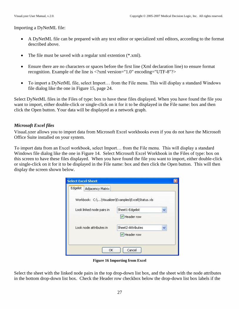
Microsoft Excel files
VisuaLyzer allows you to import data from Microsoft Excel workbooks even if you do not have the Microsoft
Office Suite installed on your system.
To import data from an Excel workbook, select Import… from the File menu. This will display a standard
Windows file dialog like the one in Figure 14. Select Microsoft Excel Workbook in the Files of type: box on
this screen to have these files displayed. When you have found the file you want to import, either double-click
or single-click on it for it to be displayed in the File name: box and then click the Open button. This will then
display the screen shown below.
Figure 16 Importing from Excel
Select the sheet with the linked node pairs in the top drop-down list box, and the sheet with the node attributes
in the bottom drop-down list box. Check the Header row checkbox below the drop-down list box labels if the

VisuaLyzer User Manual, v.2.0. Copyright 2005-2007 Medical Decision Logic, Inc. All rights reserved.
28
Excel sheets have a header row of variable names, which means the “real” data starts in the second row instead
of the first row. Finally click OK to start importing data.
If the data is in the form of an adjacency matrix, select the Adjacency Matrix tab (Fig. 17)
Figure 17 Importing adjacency matrix from Excel

VisuaLyzer User Manual, v.2.0. Copyright 2005-2007 Medical Decision Logic, Inc. All rights reserved.
29
CSV files (comma separated values)
To import data from a CSV file, select Import… from the File menu. This will display a standard Windows file
dialog like the one in Figure 14. Select CSV text in the Files of type: box on this screen to have these files
displayed. When you have found the file you want to import, either double-click on it or single-click on it for it
to be displayed in the File name: box and then click the Open button. The data will be displayed as a series of
nodes at the left hand side of the screen (Fig. 18). The nodes can then be moved and linked to show
relationships. In Figure 18, Daniel and Alyssa have been moved and linked to show a relationship. Attributes
can also be imported. Daniel was selected and double clicked to display his imported attributes.
Figure 18 Importing from CSV files

VisuaLyzer User Manual, v.2.0. Copyright 2005-2007 Medical Decision Logic, Inc. All rights reserved.
30
Opening a File
You can also open a previously saved VisuaLyzer.eng file by selecting Open… from the File menu. This will
display a screen like the one shown below.
Figure 19 Opening saved VisuaLyser files
Select VizuaLyzer files in the Files of type: box on this screen to have these files displayed. When you have
found the file you want to import, either double-click on it or single-click on it for it to be displayed in the File
name: box and then click the Open button. Your data will be displayed as a network graph.
Importing data into an existing file
If you have already created a VisuaLyzer file and wish to update the information without recreating your layout
and display settings, you can do so by importing new nodes and/or attributes. This means that if you are
conducting an ongoing study, you can import, analyze, and manipulate your data and network graph at any
point, and then update it periodically with the latest information.
Adding nodes by merging graphs
To merge two graphs, first open the graph to which new nodes will be added. An example named Tree with
EdgeAttributes.txt, from \Examples\UCINET folder, is shown in Figure 20.

VisuaLyzer User Manual, v.2.0. Copyright 2005-2007 Medical Decision Logic, Inc. All rights reserved.
31
Figure 20 Tree with edge attributes
Next select Add… from the File menu and select the file with the new nodes. This file can be in any format
accepted by VisuaLyzer. In this example Tree with EdgeAttributes-Add.txt was selected from
\Examples\UCINET folder .

VisuaLyzer User Manual, v.2.0. Copyright 2005-2007 Medical Decision Logic, Inc. All rights reserved.
32
Figure 21 Addition of nodes to existing graph
Notice the two “NewGuy” nodes in the center of the graph, connected to Hannah.
When merging graphs, VisuaLyzer will first try to match the nodes in the new file with the ones in the existing
file. If they are an exact match based on the node‟s name and attributes, they will be considered as the same
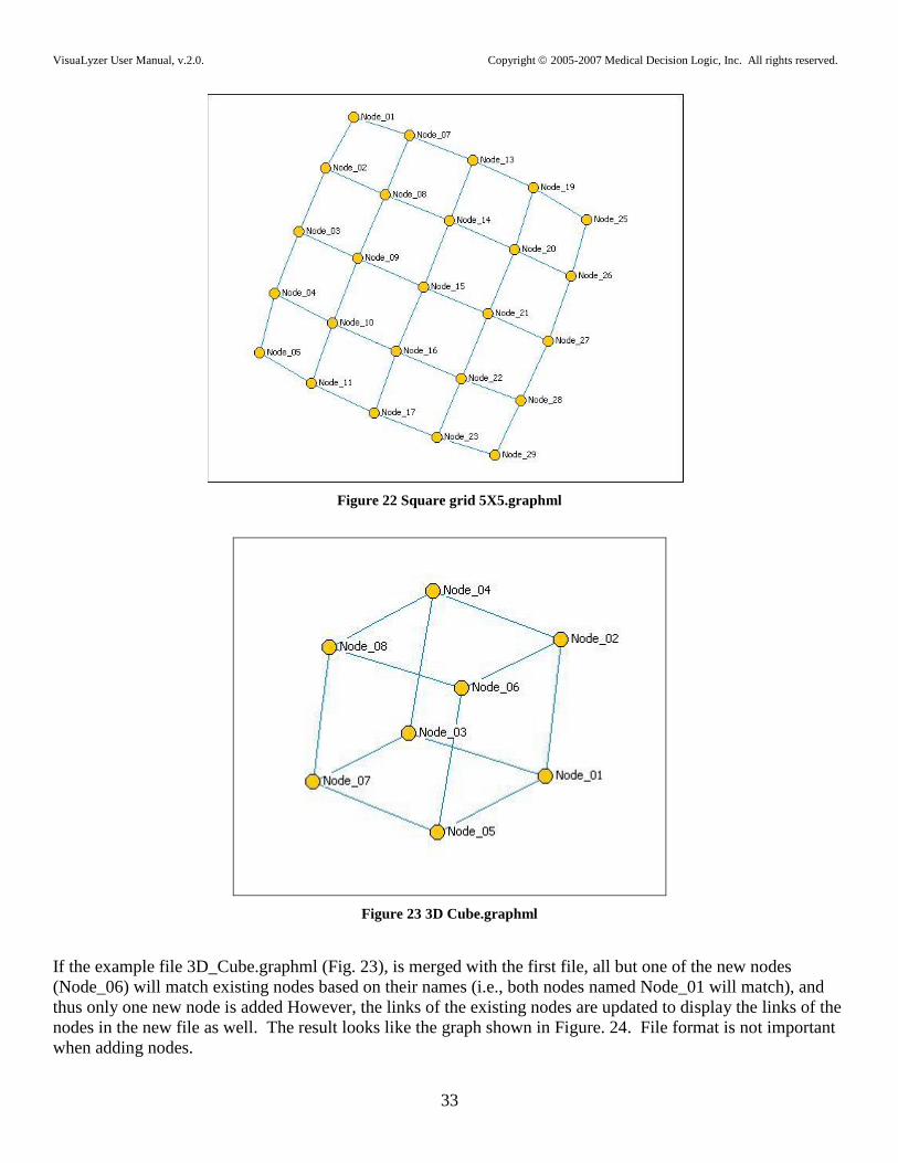
node and only the node‟s links will be updated. As an example, we will start with the example file Square grid
5x5.graphml (Fig. 22), which has 25 nodes.
VisuaLyzer User Manual, v.2.0. Copyright 2005-2007 Medical Decision Logic, Inc. All rights reserved.
33
Figure 22 Square grid 5X5.graphml
Figure 23 3D Cube.graphml
If the example file 3D_Cube.graphml (Fig. 23), is merged with the first file, all but one of the new nodes
(Node_06) will match existing nodes based on their names (i.e., both nodes named Node_01 will match), and
thus only one new node is added However, the links of the existing nodes are updated to display the links of the
nodes in the new file as well. The result looks like the graph shown in Figure. 24. File format is not important
when adding nodes.

VisuaLyzer User Manual, v.2.0. Copyright 2005-2007 Medical Decision Logic, Inc. All rights reserved.
34
Figure 24 Addition of existing nodes only adds new links
Adding new Node Attributes
You can also add new node attributes to an existing graph, which is useful if you have re-coded data or
collected new information on your existing subjects. In the previous example using the tree with edge attributes
graph (Fig. 20, page 31), each node had four attributes Age, Gender, Kids and Marry. We can add new node
attributes by selecting Add Node Attributes… from the File menu, then selecting the provided node attribute
file Tree with EdgeAttributes-AddNodeAttr.txt. The nodes will now have two additional attributes of
Education and YearsOfExperience
Note: To add node attributes, text files should be in TAB-delimited format using quotes when spaces are
present.

VisuaLyzer User Manual, v.2.0. Copyright 2005-2007 Medical Decision Logic, Inc. All rights reserved.
35
Data Export
There are several options for saving or exporting your data, each of which is described below.
Saving files
To save your data as a VisuaLyzer file, which uses a .eng extension, select Save from the File menu. If you had
previously saved the file, the file will be saved. If this is the first time you‟ve saved the file, this will bring up a
standard Windows Save screen (Fig. 25).
Figure 25 Saving data
Type the name of the file to be saved in the File name field and click the Save button.
To save a file with a different name, select Save as… from the File menu to bring up the Windows Save screen
to enter the new file name.

VisuaLyzer User Manual, v.2.0. Copyright 2005-2007 Medical Decision Logic, Inc. All rights reserved.
36
Saving images
To save your graph as an image, select Save image… from the File menu. This will bring up a standard
Windows Save screen. Type the name of the file to be saved in the File name field, select the image type you
want to save to in the Save as type drop-down list box, and click the Save button. VisuaLyzer lets you save
your graph as any of the following image types:
Monochrome bitmap (.bmp)
16 color bitmap (.bmp)
256 Color Bitmap (.bmp)
24-bit bitmap (.bmp)
JPEG (.jpg, .jpeg)
Windows Metafile (.emf)
Exporting data
Along with saving your data as a VisuaLyzer file, you can export your data to several different file types, each
of which is described below.
UCINET Edgelist1
To export your data in EdgeList1 format, select Export… from the File menu to display the standard Windows
Save screen. Type the name of the file to be saved in the File name: field, select UCINet EdgeList1 in the Save
as type: drop-down list box, and click the Save button.
UCINET Edgearray1
To export your data in EdgeArray1 format, select Export… from the File menu to display the standard
Windows Save screen. Type the name of the file to be saved in the File name: field, select UCINet EdgeArray1
in the Save as type: drop-down list box, and click the Save button.
GraphML
To export your data in GraphML format, select Export… from the File menu to display the standard Windows
save screen. Type the name of the file to be saved in the File name: field, select GraphML files in the Save as
type: drop-down list box, and click the Save button.
DyNetML
To export your data in DyNetML format, select Export… from the File menu to display the standard Windows
Save screen. Type the name of the file to be saved in the File name: field, select DyNetML files in the Save as
type: drop-down list box, and click the Save button.
Microsoft Excel
To export your data in Excel format, select Export… from the File menu to display the standard Windows Save
screen. Type the name of the file to be saved in the File name: field, select Microsoft Excel Workbook in the
Save as type: drop-down list box, and click the Save button.

VisuaLyzer User Manual, v.2.0. Copyright 2005-2007 Medical Decision Logic, Inc. All rights reserved.
37
Prolog files
To export your data in Prolog .P format, select Export… from the File menu to display the standard Windows
Save screen. Type the name of the file to be saved in the File name: field, select Prolog files in the Save as
type: drop-down list box, and click the Save button.
Adjacency Matrix
To export your data as an Adjacency Matrix, select Adjacency Matrix from the Analysis menu. An option for a
Regular (single-mode network), and one for an Affiliation (2-mode network) will pop-up. Figure 26 shown
below refers to a single-mode network.
Figure 26 Adjacency matrix screen
There are several options for saving your matrix. The matrix will be saved as you see it on the screen. You can
still edit the matrix while this window is open.
Click the button to update the matrix in the window to match the changes you made to the graph.
Click the button to save the entire matrix.
Click the button to save only the upper right half of the matrix.
Click the button to save only the lower left half of the matrix.
Click the button to fill the matrix diagonal with 0‟s.
Click the button to fill the matrix diagonal with 1‟s.
Click the button to fill the matrix diagonal with -‟s.

VisuaLyzer User Manual, v.2.0. Copyright 2005-2007 Medical Decision Logic, Inc. All rights reserved.
38
Click the button to toggle saving the node labels.
Click the button to bring up the standard Windows save screen.
Type the name of the file to be saved in the File name: field and click the Save button.
If you wish to export your adjacency matrix to Excel, set up the file as you want it and then click the export to
Excel button. This will open Excel and paste in the adjacency matrix. You can then name and save the file in
Excel.
Figure 27 shows an adjacency matrix for a simple 2-mode network showing a movie-by-actor relations.
Figure 27 Adjacency matrix for movie-by-actor affiliation network
You can save/print this matrix or export to excel following the same procedures as described above for the
single-mode network.
Display Options
Selecting nodes
There are several ways to select nodes and links in VisuaLyzer. The simplest way to select a node or link is to
click on it. If you hold down the Shift key while clicking on nodes and links, all you clicks will be selected
together.
You can also select several nodes and links by “drawing a box” around them. To do this, click on a blank part
of the graph and hold the mouse button down. This creates one corner of your box at the spot where you
clicked. Drag the opposite corner of your box to somewhere else on the screen. All links and nodes completely
contained within this box will be selected.

VisuaLyzer User Manual, v.2.0. Copyright 2005-2007 Medical Decision Logic, Inc. All rights reserved.
39
To select all nodes you can:
use Ctrl-A,
or click Select All button on the toolbar,
or use Select All in the Edit menu.
Note that whenever two nodes are selected and they have a link between them, the link will also be selected.
Graph Layout
VisuaLyzer provides several features and functions for customizing the display of your graph.
Moving nodes
To move a node, click on it and hold the mouse button down, then drag the node to where you want it and
release the mouse button. All the node‟s links will follow the node to the new location.
After moving a node, the links may not be lined up correctly – they may be bent at odd angles as they follow the
node you move. While you can manually adjust the links as described below, you can also have the program
automatically “fix” the links:
by pressing the F6 key,
or by right-clicking on the graph and selecting Straighten out links from the pop-up menu.
Selected nodes can be frozen by right-clicking on the graph screen and choosing Node(s) position > Freeze
nodes. The screen position of the selected nodes will remain unchanged even when choosing a different layout.
Nodes cannot be moved until they are unfrozen!
Moving links
VisuaLyzer also lets you control the curve of your links to help minimize line crossings. To move a link, first
click it. This will change its color and display a small drag square, or control point, (Fig. 28).
Figure 28 Moving links

VisuaLyzer User Manual, v.2.0. Copyright 2005-2007 Medical Decision Logic, Inc. All rights reserved.
40
Click on this square, hold the mouse button down, and drag it until the link is in the position you want. Then
release the mouse button. If there are multiple links between two nodes, each must be moved individually.
Spring Embedding Layout
VisuaLyzer will also automatically organize your nodes using a spring embedding layout. To use the spring
embedding layout, either
click the Spring Embedding Layout button
select Spring Embedding Layout from the Layout menu
press the F9 key
Circular Layout
VisuaLyzer allows you to automatically organize your nodes using a circular layout. To use the circular layout,
either:
click the Circular Layout button or
select Circular Layout from the Layout menu
Radial Layout
VisuaLyzer will allow you to view your nodes according to their proximity to the center of the network. To
organize your nodes using a radial layout, either:
click the Radial Layout button or
select Radial Layout from the Layout menu
Layered Layout
VisuaLyzer also allows you to organize your data according to various data values. This means that nodes can
be placed according to values along an X- and Y-axes – for example, nodes with higher values can be placed at
the top of the screen while nodes with lower values can be placed at the bottom. Using the provided example
file Tree with EdgeAttributes – Types M.eng you can load the Layered Layout setup screen shown below by
either:
clicking the Layered Layout button or
selecting “Layered Layout” from the Layout menu
Figure 29 Layered Layout setup screen

VisuaLyzer User Manual, v.2.0. Copyright 2005-2007 Medical Decision Logic, Inc. All rights reserved.
41
Nodes can also be organized along the Y-axis according to the values of their attributes. To do this, select the
radio button according to values of in the Y-axis box in the Layered Layout setup screen and then choose an
attribute in the drop-down list box and click OK. The result is shown in Figure 30.
Figure 30 Layered Layout graph

VisuaLyzer User Manual, v.2.0. Copyright 2005-2007 Medical Decision Logic, Inc. All rights reserved.
42
Selecting AGE instead of GENDER will result in the display in Figure 31.
Figure 31 Layered Layout graph 2
Now it is easy to see which nodes are oldest and youngest, and which are older and younger than others, but it is
difficult to see how they are connected because most are in the same position along the X-axis. We can “fix”
this by going back to the Layered Layout setup screen and changing the X-axis layout. We can set the X-axis to
minimize edge crossings by selecting the “based on optimization algorithm” option in the X-axis box (Fig.32).
For the Y-axis, you can organize your nodes also according to node degree (number of adjacent links) as well.
Together with the descending Sort Order option this will show nodes with more links at the top of the screen,
and nodes with fewer links at the bottom. This kind of layout makes it easy to see which nodes are the most
connected.

VisuaLyzer User Manual, v.2.0. Copyright 2005-2007 Medical Decision Logic, Inc. All rights reserved.
43
Figure 32 Layered Layout setup screen 2
Clicking OK then displays the much more readable graph shown in Figure 33.
Figure 33 Layered layout graph 3
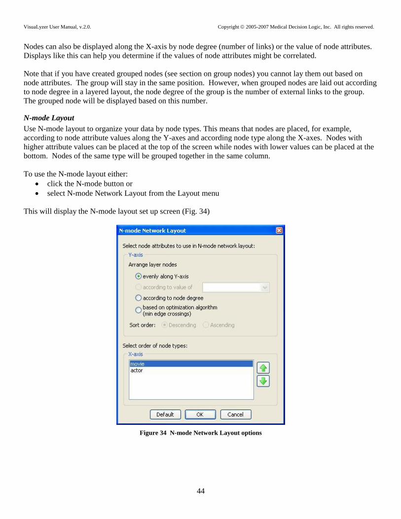
VisuaLyzer User Manual, v.2.0. Copyright 2005-2007 Medical Decision Logic, Inc. All rights reserved.
44
Nodes can also be displayed along the X-axis by node degree (number of links) or the value of node attributes.
Displays like this can help you determine if the values of node attributes might be correlated.
Note that if you have created grouped nodes (see section on group nodes) you cannot lay them out based on
node attributes. The group will stay in the same position. However, when grouped nodes are laid out according
to node degree in a layered layout, the node degree of the group is the number of external links to the group.
The grouped node will be displayed based on this number.
N-mode Layout
Use N-mode layout to organize your data by node types. This means that nodes are placed, for example,
according to node attribute values along the Y-axes and according node type along the X-axes. Nodes with
higher attribute values can be placed at the top of the screen while nodes with lower values can be placed at the
bottom. Nodes of the same type will be grouped together in the same column.
To use the N-mode layout either:
click the N-mode button or
select N-mode Network Layout from the Layout menu
This will display the N-mode layout set up screen (Fig. 34)
Figure 34 N-mode Network Layout options

VisuaLyzer User Manual, v.2.0. Copyright 2005-2007 Medical Decision Logic, Inc. All rights reserved.
45
Using the provided example file CakeHouse_2-mode.eng, this will display a 2-mode network as it is shown in
Figure 35.
Figure 35 Simple bipartite graph

VisuaLyzer User Manual, v.2.0. Copyright 2005-2007 Medical Decision Logic, Inc. All rights reserved.
46
Best Fit
As you move nodes and links around, you can automatically center them and spread them out for easier
readability by using the Best Fit feature. To use this feature, either select Best Fit from the Edit menu or click
the Best Fit button. For example, before using Best Fit a graph might look like Figure 36.
Figure 36 Cube graph
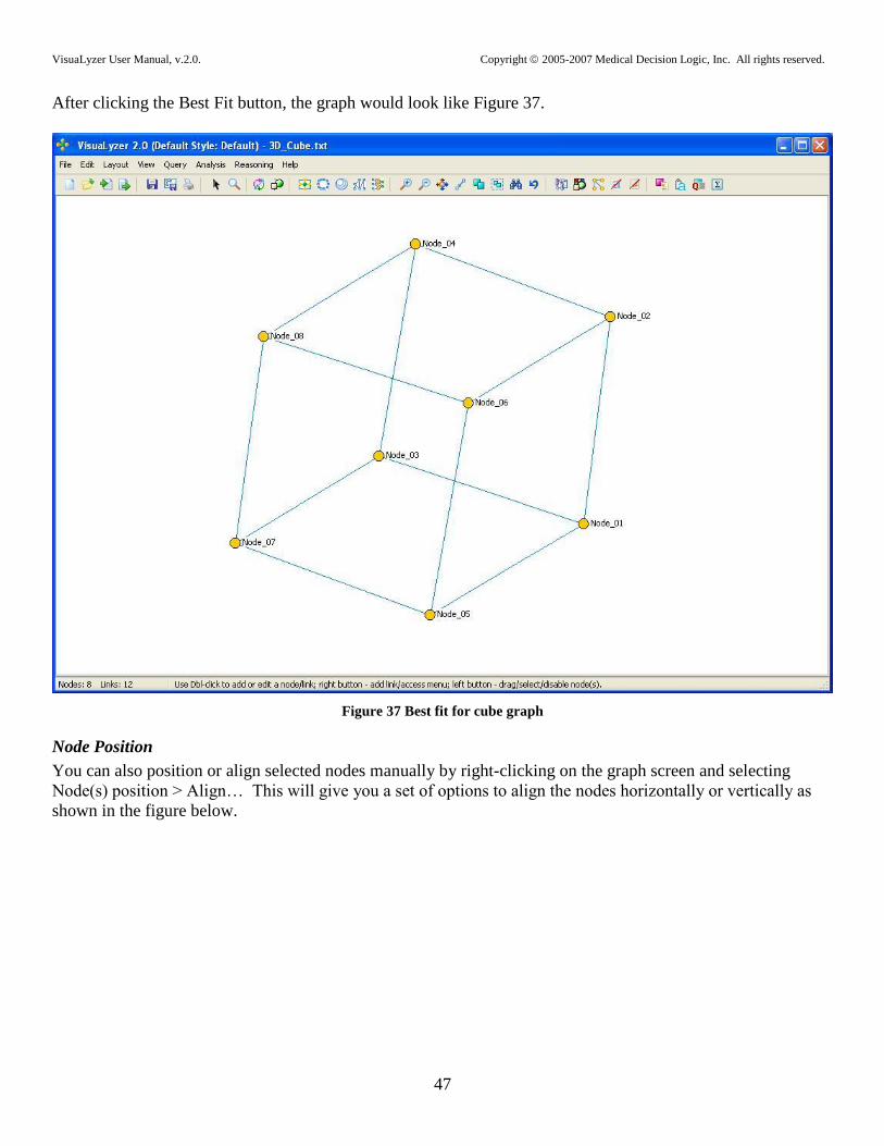
VisuaLyzer User Manual, v.2.0. Copyright 2005-2007 Medical Decision Logic, Inc. All rights reserved.
47
After clicking the Best Fit button, the graph would look like Figure 37.
Figure 37 Best fit for cube graph
Node Position
You can also position or align selected nodes manually by right-clicking on the graph screen and selecting
Node(s) position > Align… This will give you a set of options to align the nodes horizontally or vertically as
shown in the figure below.

VisuaLyzer User Manual, v.2.0. Copyright 2005-2007 Medical Decision Logic, Inc. All rights reserved.
48
Figure 38 Selected nodes position aligned
General Options
VisuaLyzer has other graph-wide display options as well. These options can be accessed and set by:
Pressing the Display Properties button
Pressing the F4 key
Selecting Edit > Display Properties > View/Edit from the main menu
This will bring up the Display Properties screen shown below.

VisuaLyzer User Manual, v.2.0. Copyright 2005-2007 Medical Decision Logic, Inc. All rights reserved.
49
Figure 39 Display properties screen
Figure 39 shows the General tab on this screen; the Nodes/Links tab will be described later.
Also note that this window can remain open on top, and moved as you work with the VisuaLyzer display. For
example, you can create and drag nodes while this window is open.
You can save your current display settings by clicking the Save button, and you can load previously saved
settings by clicking the Load button and then choosing the setting file from the standard Windows open file
screen. When you load display settings, they are applied to all nodes, links, and the background.
If at any time you wish to return to the original display, click on the Reset Display Settings button on the
toolbar. If only the last change is not desired use the Undo button.
Background color
You can change the background color for a graph by clicking on the square to the right of the Background Color
label at the top of this screen. This will open a Select Color screen. Click on a colored square and the
background of your graph will change to that color.

VisuaLyzer User Manual, v.2.0. Copyright 2005-2007 Medical Decision Logic, Inc. All rights reserved.
50
Background Image
You can also use an image for the background of your graph. To choose the image, click the rectangle to the
right of the Background Image label at the top of the General tab of the Display Properties screen. This will
bring up a standard Windows open file screen from which you can pick your background image file. Currently
VisuaLyzer allows you to use bitmaps and JPEGs as background images. Note that the aspect ratio of the
image is preserved i.e. it is not stretched to fill the screen and is centered in the display. If you have also chosen
a background color, it will be displayed it whatever space not taken up by the image To remove the background
image, click the blue word Clear beneath the Background Image label. You can also hide and unhide the
background image by un-checking or checking the Show Background Image checkbox in the middle of the
Display Properties screen.
Node color
You can control the color of nodes, created when you double-click on the screen, by changing the color of the
box to the right of the Node Color label at the top of the General tab of the Display Properties screen. This
color is changed like the background color is changed – click on the box to open the Select Color screen and
then click on a colored square to select that color. Note that changing this color does not affect the color of
existing nodes, only new ones.
Group Node Color
The color of the node representing newly grouped nodes (see group node section) can be changed by changing
the color of the box next to the Group Node Color label at the top of the General tab of the Display Properties
screen. This color is changed like the background color is changed – click on the box to open the Select Color
screen and then click on a colored square to select that color. Note that changing this color does not affect the
color of existing grouped nodes.
Selection Frame Color
When a node is selected it is surrounded by a colored square, and when a link is selected it changes to this same
color. You can change the color indicating that node or link is selected by changing the color of the box next to
the Selection Frame Color label at the top of the General tab of the Display Properties screen. This color is
changed like the background color is changed – click on the box to open the Select Color screen and then click
on a colored square to select that color. This affects both all the nodes currently in the graph and all new nodes.
Cluster Frame Color
The color of the frame (outline) of node clusters (see node cluster section) can be changed by changing the
color of the box next to the Cluster Frame Color label at the top of the Select Color screen. This color is
changed like the background color is changed – click on the box to open the Select Color screen and then click
on a colored square to select that color. Note that changing this color does not affect the color of existing
cluster frames (outlines).
Position Frame Color
The color of the frame (outline) of node position/role clusters (described below) can be changed by changing
the color of the box next to the Position Frame Color label at the top of the General tab of the Display Properties
screen. This color is changed like the background color is changed – click on the box to open the Select Color
screen and then click on a colored square to select that color. Note that changing this color does not affect the
color of existing position/role frames (outlines).

VisuaLyzer User Manual, v.2.0. Copyright 2005-2007 Medical Decision Logic, Inc. All rights reserved.
51
Show Shapes
Checking and un-checking the Show Shapes checkbox on the General tab of the Display Properties screen will
show or hide each node‟s shape. This affects both all the nodes currently in the graph and all new nodes.
Show Images
Like the graph background, nodes can also have an image as well as a color (and shape). These options are set
on the Nodes/Links tab (described below). You can hide and unhide the node images (revealing the shapes
behind them) by un-checking and checking the Show Images checkbox in the middle of the General tab of the
Display Properties screen. This affects both all the nodes currently in the graph and all new nodes.
Note that when node images are displayed they will be displayed on top of the node shape.
Note that if you uncheck both Show Shapes and Show Images that the shapes will still be displayed in order to
ensure that the node is visible.
Show Labels
Checking and un-checking the Show Labels checkbox on the General tab of the Display Properties screen will
show or hide the labels of the nodes. This affects both all the nodes currently in the graph and all new nodes.
The Toggle Off/On button on the tool bar can also be used to turn the labels off and on.
Show Borders
Checking and un-checking the Show Borders checkbox on the General tab of the Display Properties screen will
show or hide a thin black border line around each node. This affects both all the nodes currently in the graph
and all new nodes.
Show Disabled Nodes
When a node or link is disabled (described below) it is displayed as light gray. To completely hide disabled
nodes, un-check the Show Disabled Nodes checkbox on the General tab of the Display Properties screen.
Checking this box will again cause disabled nodes and links to be displayed in light gray. This affects both all
the nodes currently in the graph and all new nodes.
Show ToolTips
When the Show ToolTips check box on the General tab of the Display Properties screen is checked, a node‟s or
link‟s attributes and values will be displayed as a yellow tool tip when the cursor is held over them. When this
box is not checked, this information will not be displayed. This affects both all the nodes/links currently in the
graph and all new node/links.
Show Links
When the Show Links checkbox on the General tab of the Display Properties screen is checked, all links will be
displayed. When this box is not checked, links will not be displayed. This affects both all the links currently in
the graph and all new links.
Show Link Arrow
When the Show Link Arrows checkbox on the General tab of the Display Properties screen is checked, all
directed links will have an arrowhead indicating the To Node of the link. When this box is not checked, no
links will have arrowheads. This affects both all the links currently in the graph and all new links.
VisuaLyzer User Manual, v.2.0. Copyright 2005-2007 Medical Decision Logic, Inc. All rights reserved.
52
Show Link Type (relation)
When the Show Link Type checkbox on the General tab of the Display Properties screen is checked, all links
will be labeled with their type (as defined on the Edit Link screen). When this box is not checked, these types
will not be displayed. This affects both all the links currently in the graph and all new links.
Show Link Label
When the Show Link Label checkbox on the General tab of the Display Properties screen is checked, all links
will be labeled with their Label property (as defined on the Edit Link screen). When this box is not checked,
these labels will not be displayed. This affects both all the links currently in the graph and all new links.
Show Link Weight
When the Show Link Weight checkbox on the General tab of the Display Properties screen is checked, all links
will be labeled with their Weight property (as defined on the Edit Link screen). When this box is not checked,
these values will not be displayed. This affects both all the links currently in the graph and all new links.
AutoOrganize
When the AutoOrganize checkbox on the General tab of the Display Properties screen is checked, every time a
node is moved or a link is added the graph will automatically organize itself according to the last selected
automatic layout (spring embedded, circular, or layered). When this box is not checked, nodes and links will
stay where they are placed.
Animation
When the Animation checkbox on the General tab of the Display Properties screen is checked, each time a
layout is applied (including via the AutoOrganize feature) both the nodes and the links will be shown moving
from their current positions to their final positions. When this box is not checked, nodes and links will simply
“snap” to their final positions.
Sounds Effects
When the Sound Effects checkbox on the General tab of the Display Properties screen is checked, certain
actions, such as automatic layouts, will be accompanied by sound effects. When this box is not checked, no
functions will be accompanied by sounds.
Node options
VisuaLyzer provides several options for displaying nodes. These options can be accessed and set by:
Pressing the Display Properties button
Pressing the F4 key
Selecting Edit > Display Properties > View/Edit from the main menu
This will bring up the Display Properties screen for Nodes/Links (Figure 40).

VisuaLyzer User Manual, v.2.0. Copyright 2005-2007 Medical Decision Logic, Inc. All rights reserved.
53
Figure 40 Display properties Nodes/Links
Note that we are looking at the Nodes/Links tab on this screen; the General tab was described earlier. This
screen shows the information for the currently selected node(s). No nodes were selected when the above screen
shot was taken, thus there are no values are displayed. No value information is also displayed when multiple
nodes are selected and have conflicting values (e.g., they are different colors or shapes). When a node is
selected, the Nodes/Links tab would look something like Figure 41.

VisuaLyzer User Manual, v.2.0. Copyright 2005-2007 Medical Decision Logic, Inc. All rights reserved.
54
Figure 41 Node properties on display screen
Again, note that this window can remain open (and on top) as you work with the VisuaLyzer display. For
example, you can create and drag nodes while this window is open. When you select a node or nodes when this
tab is open, the information on the tab will be updated to reflect the display information for the selected node(s).
Color
You can change the color of the selected nodes(s) by clicking on the square to the right of the Color label in the
Nodes section at the top of the Nodes/Links tab of the Display Properties screen. This will open a Select Color
screen. Click on a colored square and the selected node(s) will change to that color.
Shape
You can change the shape of the selected nodes(s) by clicking on the shape (or blank box) to the right of the
Shape label in the Nodes section at the top of the Nodes/Links tab of the Display Properties screen, and then
clicking on a shape from the Select Shape screen that is displayed (Fig. 42).

VisuaLyzer User Manual, v.2.0. Copyright 2005-2007 Medical Decision Logic, Inc. All rights reserved.
55
Figure 42 Select shape screen
Clicking on the A on the Select Shape screen, (assuming that all nodes are selected), will cause the node‟s label
to be used as the shape – this means that the label will be centered between any links to those nodes, as shown
below.
Figure 43 Node labels used as node shapes
Note that when node images are displayed they will be displayed on top of the node shape, except when the
label is the shape.

VisuaLyzer User Manual, v.2.0. Copyright 2005-2007 Medical Decision Logic, Inc. All rights reserved.
56
Image
You can change the image displayed for the selected nodes(s) by clicking on the image (or blank box) to the
right of the Image label in the Nodes section at the top of the Nodes/Links tab of the Display Properties screen.
There are 15 predefined images to choose from, or you may load a bitmap or JPEG image file of your choice.
To make the selected image transparent, thus showing the node shape or background behind it, check the
Transp. checkbox below the word Image. To remove the image completely, click the blue word Clear below
the Transp. Checkbox. Note that when node images are displayed they will be displayed on top of the node
shape, except when the label is the shape.
Size
You can change the size of the selected nodes(s) by typing a number (representing a number of pixels) in the
field to the right of the Size, pixels label in the Nodes section at the top of the Nodes/Links tab of the Display
Properties screen and then pressing the Enter key. You can also change the size of the selected node(s) by using
the up and down arrow keys on your keyboard.
Label Orientation
You can change the label orientation (where the label is in relation to the node) of the selected nodes(s) by
selecting a choice from the drop-down list box to the right of the Label Orientation label in the Nodes section at
the top of the Nodes/Links tab of the Display Properties screen.
Font
To change the font of the label of the selected nodes(s), click the letters (or blank space) to the right of the Font
label in the Nodes section at the top of the Nodes/Links tab of the Display Properties screen. This will display a
screen like the one shown below.
Figure 44 Font selection screen
Select the options you want for the font and then click the OK button to change the node label(s).

VisuaLyzer User Manual, v.2.0. Copyright 2005-2007 Medical Decision Logic, Inc. All rights reserved.
57
Disabling Nodes
If you are interested in seeing what your data would be like (such as layout or network analyses) without a
certain node or nodes, you can do so without having to delete the node(s) and then re-enter them again later.
When a node (and its links) is disabled, it is not used for determining layouts or other analyses; (discussed
below).
There are two quick ways to disable (and later re-enable) nodes:
Select one or more nodes and press the Delete key
Hold down the CTRL key and click on a node
You can also select Enable nodes… from the Edit menu to display the Enable Nodes screen (Figure 45).
Figure 45 Enable nodes screen
By default, nodes that are checked are enabled. To disable the nodes, uncheck the box next to that node‟s name.
Click the Enable Selected button to enable all selected nodes (and disable all other nodes). Click the Disable
Selected button to disable all selected nodes (and enable all other nodes). Clicking the Enable All or Disable
All buttons will enable or disable all nodes in the graph, respectively. Disabled nodes can be moved manually,
but are ignored by the automatic layout routines (including AutoOrganize). You can also edit disabled nodes
and links.
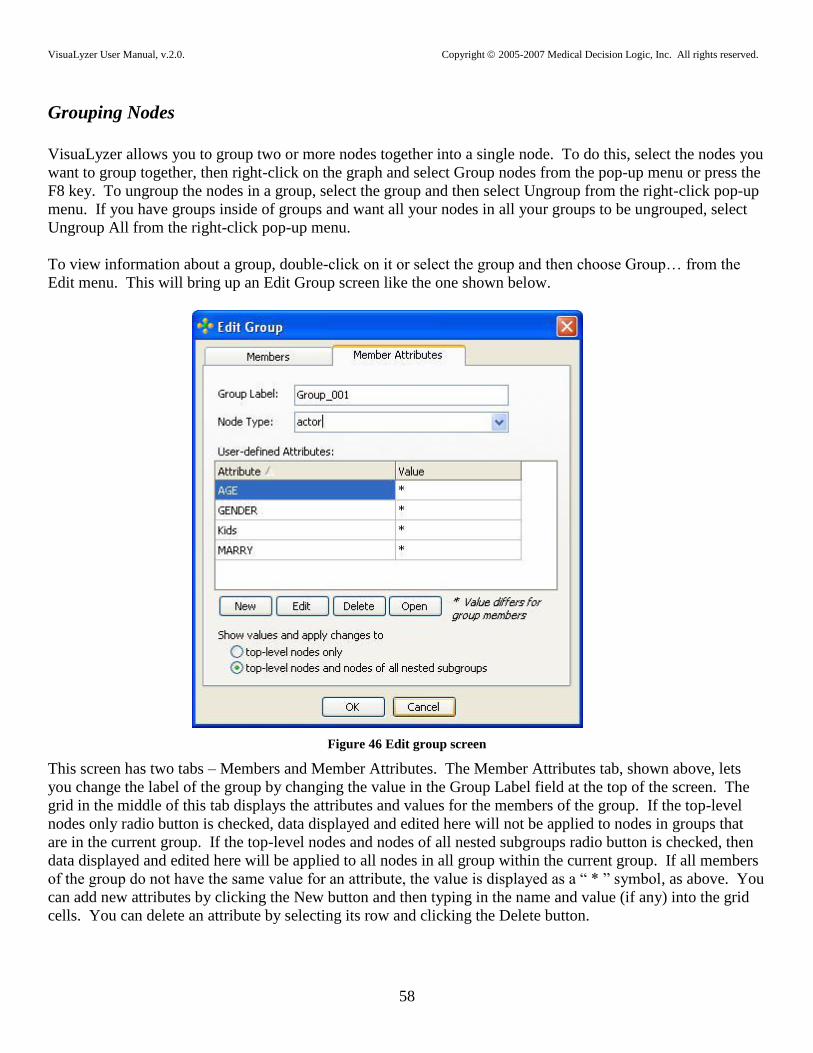
VisuaLyzer User Manual, v.2.0. Copyright 2005-2007 Medical Decision Logic, Inc. All rights reserved.
58
Grouping Nodes
VisuaLyzer allows you to group two or more nodes together into a single node. To do this, select the nodes you
want to group together, then right-click on the graph and select Group nodes from the pop-up menu or press the
F8 key. To ungroup the nodes in a group, select the group and then select Ungroup from the right-click pop-up
menu. If you have groups inside of groups and want all your nodes in all your groups to be ungrouped, select
Ungroup All from the right-click pop-up menu.
To view information about a group, double-click on it or select the group and then choose Group… from the
Edit menu. This will bring up an Edit Group screen like the one shown below.
Figure 46 Edit group screen
This screen has two tabs – Members and Member Attributes. The Member Attributes tab, shown above, lets
you change the label of the group by changing the value in the Group Label field at the top of the screen. The
grid in the middle of this tab displays the attributes and values for the members of the group. If the top-level
nodes only radio button is checked, data displayed and edited here will not be applied to nodes in groups that
are in the current group. If the top-level nodes and nodes of all nested subgroups radio button is checked, then
data displayed and edited here will be applied to all nodes in all group within the current group. If all members
of the group do not have the same value for an attribute, the value is displayed as a “ * ” symbol, as above. You
can add new attributes by clicking the New button and then typing in the name and value (if any) into the grid
cells. You can delete an attribute by selecting its row and clicking the Delete button.

VisuaLyzer User Manual, v.2.0. Copyright 2005-2007 Medical Decision Logic, Inc. All rights reserved.
59
To view the Members tab, click the Members tab at the top of the Edit Group screen. This will display a screen
like the one shown below.
Figure 47 Edit group screen - members
Again, you can change the name of the group by changing the value in the Group Name field at the top of the
screen. The list on the left contains all nodes and groups in the current graph. The list on the right contains all
nodes and groups that are members of the current group. To add a node or group to the current group, select
that node or group in the left-hand list and click the Add button, or drag and drop the node into the Group
members list. To remove a node or group from the current group, select that node or group in the right-hand list
and click the Remove button.
Link options
VisuaLyzer provides several options for displaying links. These options can be accessed and set by:
Pressing the Display Properties button
Pressing the F4 key
Selecting Edit > Display Properties > View/Edit from the main menu
This will bring up the Display Properties screen. To access the Nodes/Links tab, click on the Nodes/Links tab
at the top of the screen (see Figure 41). Also note that this screen reflects the information for the currently
selected link(s). No links were selected when the above screen shot was taken, thus there are no values
displayed. No value information is also displayed when multiple links are selected and have conflicting values

VisuaLyzer User Manual, v.2.0. Copyright 2005-2007 Medical Decision Logic, Inc. All rights reserved.
60
(e.g., they are different colors or widths). When a link is selected, the Nodes/Links tab would look something
like the screen shown below.
Figure 48 Display properties screen - links
This window can remain open (and on top) as you work with the VisuaLyzer display. For example, you can
create and drag links while this window is open. When you select a link or links when this tab is open, the
information on the tab will be updated to reflect the display information for the selected link(s).
Color
You can change the color of the selected link(s) by clicking on the square to the right of the Color label in the
Links section at the bottom of the Nodes/Links tab of the Display Properties screen. This will open a Select
Color screen. Click on a colored square and the selected link(s) will change to that color.
Width
You can change the width or thickness of the selected link(s) by entering a number (representing a number of
pixels) in the field to the right of the Width, pixels label in the Links section at the bottom of the Nodes/Links
tab of the Display Properties screen and then pressing the Enter key.

VisuaLyzer User Manual, v.2.0. Copyright 2005-2007 Medical Decision Logic, Inc. All rights reserved.
61
Style
You can change the style of the selected link(s) by selecting a line type in the drop-down list box to the right of
the Style label in the Links section at the bottom of the Nodes/Links tab of the Display Properties screen.
Selection of a style will only affect links with a pixel width of 1.
Font
You can change the font of the labels of the selected link(s) by clicking on the letters (or blank space) to the
right of the Font label in the Links section at the bottom of the Nodes/Links tab of the Display Properties
screen. This will display a font selection screen (Figure 44). Select the options you want for the font and then
click the OK button to change the link label(s).
Arrowhead Color
You can change the color of the arrowheads of the selected link(s) by clicking on the colored square to the right
of the Arrow Head Color label in the Links section at the bottom of the Nodes/Links tab of the Display
Properties screen, and then selecting a color from the Select Color screen that is displayed. This is similar to
selecting colors for other options previously described.
Head Length
You can change the length of the arrow heads of the selected link(s) by entering a number (representing a
number of pixels) in the field to the right of the Head Length, pixels label in the Links section at the bottom of
the Nodes/Links tab of the Display Properties screen and then pressing the Enter key.
Head Width
You can change the width of the arrow heads of the selected link(s) by entering a number (representing a
number of pixels) in the field to the right of the Head Width, pixels label in the Links section at the bottom of
the Nodes/Links tab of the Display Properties screen and then pressing the Enter key.
Grouping Links
VisuaLyzer allows you to set attributes and attribute values for groups of links. To do this, select the links you
want to group, then right-click on the graph and select Group links… from the pop-up menu. This will bring up
an Edit Group of Links screen like the one shown below.
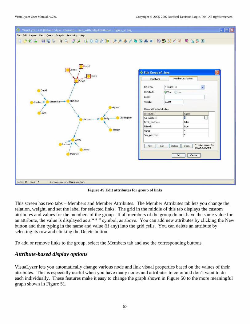
VisuaLyzer User Manual, v.2.0. Copyright 2005-2007 Medical Decision Logic, Inc. All rights reserved.
62
Figure 49 Edit attributes for group of links
This screen has two tabs – Members and Member Attributes. The Member Attributes tab lets you change the
relation, weight, and set the label for selected links. The grid in the middle of this tab displays the custom
attributes and values for the members of the group. If all members of the group do not have the same value for
an attribute, the value is displayed as a “ * ” symbol, as above. You can add new attributes by clicking the New
button and then typing in the name and value (if any) into the grid cells. You can delete an attribute by
selecting its row and clicking the Delete button.
To add or remove links to the group, select the Members tab and use the corresponding buttons.
Attribute-based display options
VisuaLyzer lets you automatically change various node and link visual properties based on the values of their
attributes. This is especially useful when you have many nodes and attributes to color and don‟t want to do
each individually. These features make it easy to change the graph shown in Figure 50 to the more meaningful
graph shown in Figure 51.

VisuaLyzer User Manual, v.2.0. Copyright 2005-2007 Medical Decision Logic, Inc. All rights reserved.
63
Figure 50 Basic graph

VisuaLyzer User Manual, v.2.0. Copyright 2005-2007 Medical Decision Logic, Inc. All rights reserved.
64
Figure 51 Adding meaning to a basic graph
The process for changing the first graph to look like the second is described below.
Node Label
To base node labels upon the value of one of the nodes‟ attributes:
select Query > Attribute Based > Label…
or click the Attribute Based Query button and select the Label tab.
This will display the Label tab of the Attribute Based… screen (Fig.52).

VisuaLyzer User Manual, v.2.0. Copyright 2005-2007 Medical Decision Logic, Inc. All rights reserved.
65
Figure 52 Attribute base selection screen
The default is to label nodes with the value of their Label property, but you can have the nodes labeled with the
value of any of their attributes. Select the attribute whose value you want used as a label in the drop-down list
box at the top of this screen and then click the Apply button.
Node Color
To have the node color based upon the value of one of the nodes‟ attributes:
select Query > Attribute Based > Color…
or click the Attribute Based Query button and select the Color tab
This will display the Color tab of the Attribute Based… screen. Select the attribute you want used to determine
color in the drop-down list box at the top of this screen. The Legend box will then be filled with a list of the
values for that attribute, with a colored square next to each value indicating the color that will be used for nodes
with that value (Fig.53).

VisuaLyzer User Manual, v.2.0. Copyright 2005-2007 Medical Decision Logic, Inc. All rights reserved.
66
Figure 53 Attribute based selection screen - color tab
You can change the color used for an attribute value by:
selecting an attribute value label or colored square to the left, clicking the Select… button
double clicking on label or colored square
using Ctrl/Shift to select group of values
using collapsed values (see figure below)
and select the new color from the color palette.
When the Collapse Values button is selected, the resulting dialogue window allows you to specify the start
value, end value and the desired color for the group of nodes (Fig.54).
Note: The preceding process can be applied to node shape, node size and link color data as well.
To apply colors to the nodes on the screen, click Apply. Note that the Show Image box on the General tab in
the Display Properties selection screen should be un-checked.
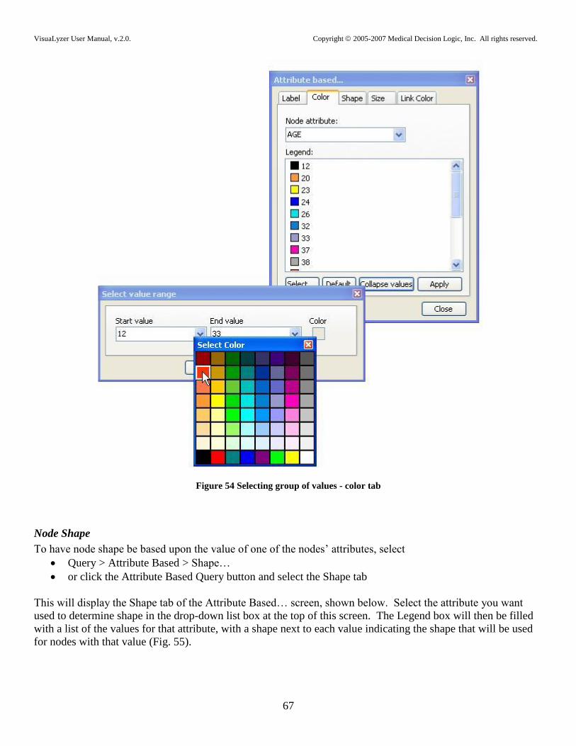
VisuaLyzer User Manual, v.2.0. Copyright 2005-2007 Medical Decision Logic, Inc. All rights reserved.
67
Figure 54 Selecting group of values - color tab
Node Shape
To have node shape be based upon the value of one of the nodes‟ attributes, select
Query > Attribute Based > Shape…
or click the Attribute Based Query button and select the Shape tab
This will display the Shape tab of the Attribute Based… screen, shown below. Select the attribute you want
used to determine shape in the drop-down list box at the top of this screen. The Legend box will then be filled
with a list of the values for that attribute, with a shape next to each value indicating the shape that will be used
for nodes with that value (Fig. 55).
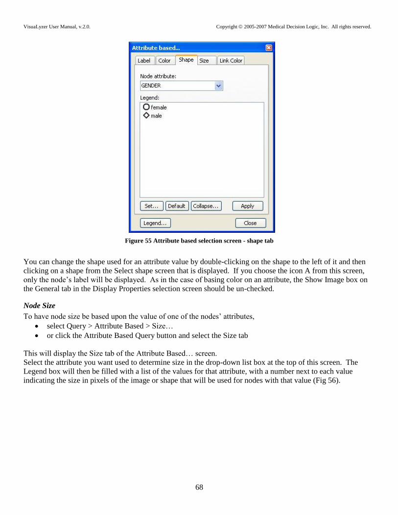
VisuaLyzer User Manual, v.2.0. Copyright 2005-2007 Medical Decision Logic, Inc. All rights reserved.
68
Figure 55 Attribute based selection screen - shape tab
You can change the shape used for an attribute value by double-clicking on the shape to the left of it and then
clicking on a shape from the Select shape screen that is displayed. If you choose the icon A from this screen,
only the node‟s label will be displayed. As in the case of basing color on an attribute, the Show Image box on
the General tab in the Display Properties selection screen should be un-checked.
Node Size
To have node size be based upon the value of one of the nodes‟ attributes,
select Query > Attribute Based > Size…
or click the Attribute Based Query button and select the Size tab
This will display the Size tab of the Attribute Based… screen.
Select the attribute you want used to determine size in the drop-down list box at the top of this screen. The
Legend box will then be filled with a list of the values for that attribute, with a number next to each value
indicating the size in pixels of the image or shape that will be used for nodes with that value (Fig 56).

VisuaLyzer User Manual, v.2.0. Copyright 2005-2007 Medical Decision Logic, Inc. All rights reserved.
69
Figure 56 Attribute selection screen - size tab
You can change the size used for an attribute value by double-clicking on the number to the left of it and then
entering a number in the field on the Size screen that is displayed.
Link Color
To have link color be based upon the value of one of the links‟ attributes,
select Query > Attribute Based > Link Color…
or click the Link color by Attribute icon.
This will display the Link Color tab of the Attribute Based… screen. Select the attribute you want used to
determine link color in the drop-down list box at the top of this screen. The Legend box will then be filled with
a list of the values for that attribute, with a colored square next to each value indicating the color that will be
used for links with that value (Fig. 57)

VisuaLyzer User Manual, v.2.0. Copyright 2005-2007 Medical Decision Logic, Inc. All rights reserved.
70
Figure 57 Attribute based selection screen - link color tab
You can change the color used for an attribute value by double-clicking on the colored square to the left of it
and then clicking on a color from the Select Color screen that is displayed.
Legend for attribute-based queries
The legend window displays the last attribute queries for node label, color, shape, and size and link color
(Figure 58). The legend can be saved as a bitmap or JPG image and used later in conjunction with the graph
image in presentations.
Query-based attribute settings cannot “coexist” with a change in the attribute for even one node via the Display
Settings form. Should you attempt to effect a change a warning to this effect will be received.

VisuaLyzer User Manual, v.2.0. Copyright 2005-2007 Medical Decision Logic, Inc. All rights reserved.
71
Figure 58 Legend window
Views
A view consists of the last set of attribute queries, which can be saved and later applied to the same or other
data. This allows you, for instances, to retain a uniform look and feel for the results of many interviews
conducted in the course of a study. The command to save or to load is under the Query/Views menu (Fig 59)
figure below).
It is recommended that views be named according to the effect they produce.

VisuaLyzer User Manual, v.2.0. Copyright 2005-2007 Medical Decision Logic, Inc. All rights reserved.
72
Figure 59 Loading and saving views
Display Relations/Types
Since VisuaLyzer allows multiple link types (relations), you can choose to show any number of these relations
as well as the color of each of them. To control which relations are shown and their colors, select Select
Relation… from the View menu or click the Select Relation button. This will display a Relation tab on Select
Relation/Type screen (Fig. 60.)

VisuaLyzer User Manual, v.2.0. Copyright 2005-2007 Medical Decision Logic, Inc. All rights reserved.
73
Figure 60 Select relation/links
The top part of the screen indicates which relations are being displayed and the color of the links for each.
Check or un-check the checkbox next to a relation to show or hide that relation (link) in the network graph. For
example, in Figure 60 three link types are shown. The lower part of the screen refers to link attributes. In the
case being considered, the links have no attributes. Suppose, however, that the graph showed only one relation
“is linked to”, had been assigned an attribute of “friend” with values of True or False. “Friend” would have
been listed in the Link attribute drop down box and the choices of True, False and “na” in the Select Attribute
Value(s) panel. Clicking the check box next to true would have shown links to all the people who were friends.
You can change the color used for an attribute value by double-clicking on the colored square to the left of it,
clicking on a color from the Select Color screen that is displayed, and then clicking the Apply Colors button.
Similarly, since VisuaLyzer allows multiple node types (actors, events, etc.), you can choose to enable or select
nodes of specified types. Selecting nodes is useful for setting visual and custom attributes for a group of nodes.
Enable/Disable helps to explore affiliations in the network and conduct “What if…” types of analysis.
To control which node types are shown and their colors, select Select “Type of node” tab on the Select
Relation/Type screen from the View menu or click the Select type of node button. This will display the Type of
node tab on Select Relation/Type screen (Fig. 61)

VisuaLyzer User Manual, v.2.0. Copyright 2005-2007 Medical Decision Logic, Inc. All rights reserved.
74
Figure 61 Select type of node
The lower part of the screen refers to node attributes and works as described above for the Relation (type of
link) tab. However the action choices on this tab are enable/select, rather than show/hide.
Graph Animation
VisuaLyzer allows you to animate your networks by displaying several .eng files sequentially, similar to a
cartoon flipbook. All files involved in the animation sequence must be located in the same directory.
VisuaLyzer will display all files in the chosen directory in alphabetical order. To animate a series of graphs,
select Animate Sequence… from the File menu. This will display the Network Animator screen shown below.

VisuaLyzer User Manual, v.2.0. Copyright 2005-2007 Medical Decision Logic, Inc. All rights reserved.
75
Figure 62 Network animator
Select the directory where the files are located by either typing the path in the Working folder field or clicking
the “…” button to the right of this field and selecting the directory from the Windows directory tree that is
displayed. Indicate the number of files to be displayed per second in the Rate field. Check the Cyclic playback
checkbox if you want the series of files to be displayed over and over, continuously. Click the Play button to
play the sequence, and click the Stop button to stop the sequence from playing. Clicking the “<<” button will
display the first frame in the sequence, and clicking the “>>” button will display the last frame in the sequence.
Clicking the “<” button will display the previous frame in the sequence, and clicking the “>” button will display
the net frame in the sequence.

VisuaLyzer User Manual, v.2.0. Copyright 2005-2007 Medical Decision Logic, Inc. All rights reserved.
76
Data or Network Querying
Queries enable selection of nodes or links that fit specific criteria set by the researcher VisuaLyzer implements
two types of queries: nodes search and linked pairs comparison.
Node search
Node search queries find nodes or links that satisfy criteria set a priori by the researcher. Let‟s take the
Krackhardt‟s high tech example. A researcher interested in career trajectories of young executives may want to
find the young (e.g., under 40 yrs) managers in the company‟s advice network.
To execute this query, load the Krackhardt‟s advice network and select Search Query from the Query menu.
This will bring up a window like the one shown below.
Figure 63 Node search
1. Select the basis of
the query: node or
link attributes
3. Set the conditions:
Select an attribute of interest from the drop down box (under the
attribute column).
Select a mathematical function (e.g., less than, greater than, equal to, etc).
Select a value for the attribute.
You can perform Boolean queries, based on multiple attributes.
In the example above, the query selects nodes that are younger than 40
years old AND who are at level 2 (managers) of the corporate hierarchy.
Click Submit to execute the query. This will present the results in a graph
like the one shown below.
2. Select node state – whether you
want the nodes enabled, disabled or
selected
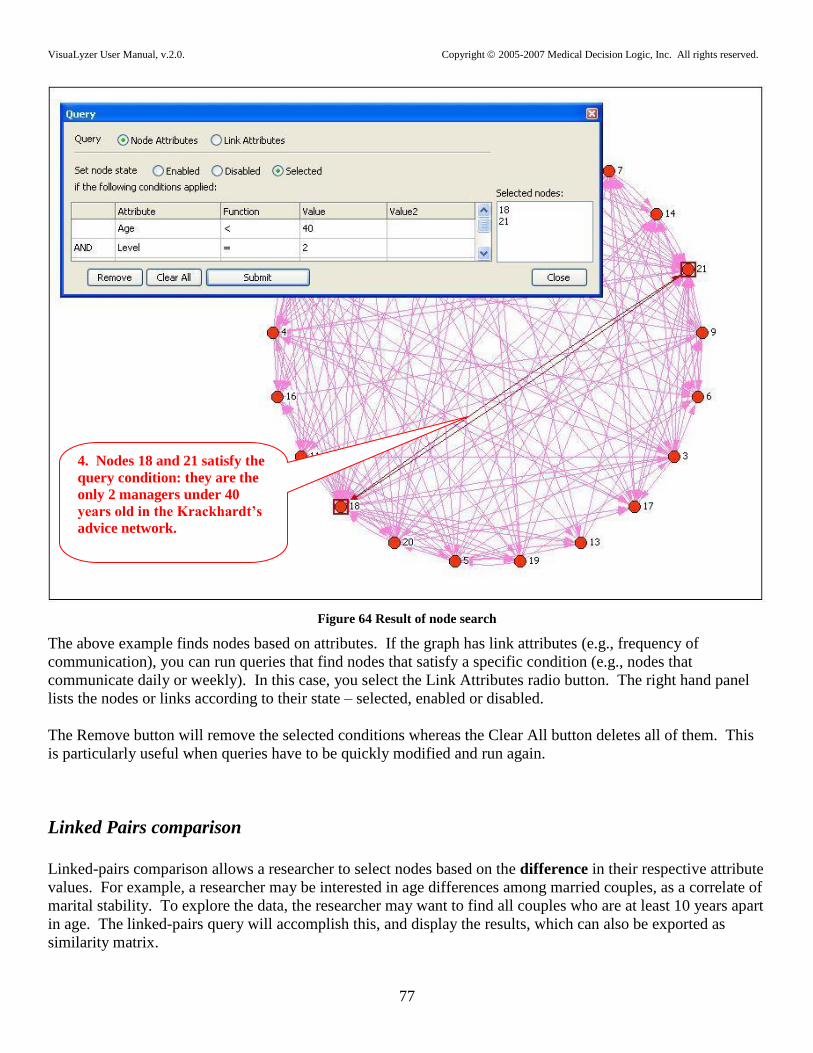
VisuaLyzer User Manual, v.2.0. Copyright 2005-2007 Medical Decision Logic, Inc. All rights reserved.
77
Figure 64 Result of node search
The above example finds nodes based on attributes. If the graph has link attributes (e.g., frequency of
communication), you can run queries that find nodes that satisfy a specific condition (e.g., nodes that
communicate daily or weekly). In this case, you select the Link Attributes radio button. The right hand panel
lists the nodes or links according to their state – selected, enabled or disabled.
The Remove button will remove the selected conditions whereas the Clear All button deletes all of them. This
is particularly useful when queries have to be quickly modified and run again.
Linked Pairs comparison
Linked-pairs comparison allows a researcher to select nodes based on the difference in their respective attribute
values. For example, a researcher may be interested in age differences among married couples, as a correlate of
marital stability. To explore the data, the researcher may want to find all couples who are at least 10 years apart
in age. The linked-pairs query will accomplish this, and display the results, which can also be exported as
similarity matrix.
4. Nodes 18 and 21 satisfy the
query condition: they are the
only 2 managers under 40
years old in the Krackhardt’s
advice network.

VisuaLyzer User Manual, v.2.0. Copyright 2005-2007 Medical Decision Logic, Inc. All rights reserved.
78
So, let‟s take the Krackhardt advice network. Our interest is in finding out age difference or asymmetry in
advice relations (i.e., the extent to which people seek advice from others who are older or younger than them).
To execute this query, load the Krackhardt‟s advice network and select Linked Pairs Comparison from the
Query menu. This will bring up a window like the one shown below.
Figure 65 Linked pairs comparison
3. Set the conditions:
Select an attribute of interest from the drop down box (under the attribute
column). – here Age
Select a mathematical function (e.g., less than, greater than, equal to, etc) –
here greater than since we want to find the difference of 20 years
Set the comparison (or difference) value for the attribute – here 20 years.
You can perform Boolean queries, based on multiple attributes
In the example above, the query selects pairs of nodes that are more than
20 years apart in age.
Click Submit to execute the query. This will present the results in a graph like
the one shown below

VisuaLyzer User Manual, v.2.0. Copyright 2005-2007 Medical Decision Logic, Inc. All rights reserved.
79
Figure 66 Results of linked pairs comparison
The results of the linked-pairs comparison can be represented as a binary similarity matrix for further
analysis/processing. The cells in the matrix take the value of 1, if the age difference between pairs of nodes is
greater than 20 years.
Query History
The Query History window presents a list of previous queries: these can be edited and/or resubmitted for
analysis.

VisuaLyzer User Manual, v.2.0. Copyright 2005-2007 Medical Decision Logic, Inc. All rights reserved.
80
ANALYZING SOCIAL NETWORK DATA
Network Level Properties
Visualyzer provides a number of network properties by default. To see these properties, follow these steps:
1. Open any network graph (.eng file). E.g. Krackhardt‟s HighTech Advice network graph.
2. Select Network Properties from the Analysis menu to open the Network Properties form, (Fig. 67).
Figure 67 Network Properties
Total nodes: Total number of nodes in current network(s). For example, there are 21 nodes in the
advice network, and all nodes are enabled.
Enabled Nodes: Number of the nodes that are enabled. Disabled nodes are ignored in calculation of
parameters.

VisuaLyzer User Manual, v.2.0. Copyright 2005-2007 Medical Decision Logic, Inc. All rights reserved.
81
Isolate Nodes: Number of isolates in the currently displayed graph, if any.
Groups: Groups are collection of nodes sharing similar attributes. For example, a network can be
broken into two groups of male and female network members. The Groups parameter
indicates the total number of grouped nodes in the current network. A group can contain
1 or more other nodes or groups. (For details on how to construct groups, see section
Grouping Nodes).
Relations: In VisuaLyzer, a network graph (eng file) can consist of single or multiple relations (or
link types). Operations including calculation of parameters can be restricted to any or all
of these relations at any given time. The Relations parameter indicates the link types in
the graph, even if they are not displayed or have been disabled. For example, the
Krackhardt High-Tech dataset contains three relations: ADVICE, FRIENDSHIP and
REPORTS_TO, but only the ADVICE relation is currently in focus and displayed, hence
it is indicated in the Current relations value.
Current Relations: Similar to the Relations, the Current Relations parameter indicates the “link type” or
relation under current consideration, e.g., ADVICE relations.
Total links: This is the total number of links (or edges or connections) in all relations in the current
graph, regardless of whether relations are enabled or not. For example, all three relations
in the Krackhardt High-Tech data set produce 312 links.
Current links Total number of links in currently selected networks (or number of visible links). This
includes links connecting both enabled and disabled nodes (a link could be
enabled/disabled by disabling its corresponding nodes).
Current Enabled links: The Enabled links value indicates the number of the links that are enabled in the current
network. Disabled links are ignored during calculations (a link is disabled if any of the
connected nodes are disabled).
Diameter: The longest geodesic distance within the network (unless infinite). The diameter of a
graph is important because it quantifies how far apart the farthest two nodes in the graph
are, and therefore how long it would take to reach that node – e.g., the furthest
(maximum) distance a message would have to travel from node i to node j.
(Geodesic) Distance: A pair of nodes could be connected by several paths or links, which may differ in length.
A shortest path between two nodes is referred to as a geodesic. If there is more than one
shortest path between a pair of nodes, then there are two geodesics between them. Thus,
the geodesic (distance) between two nodes is defined as the length of the geodesic
between them. For valued graphs, the geodesic distance is the cheapest or shortest path
between points, computed by summing the values of each link in the path. Distances are
relevant in social network analysis because they indicate how far apart nodes are.
Density: Proportion of links that are actually present in a graph. It is the ratio of total number of
links to the maximum possible links. For an all to all connected network Density = 1.0.
For valued graphs, density is the average proportion of links or mean degree of nodes in a
graph.

VisuaLyzer User Manual, v.2.0. Copyright 2005-2007 Medical Decision Logic, Inc. All rights reserved.
82
Centralization: Overall network degree centralization measures the extent to which a single actor has
high centrality, and the others low centrality. The larger the centralization score, the
more likely it is that a single actor is quite central with the remaining actors considerably
less central, and probably at the periphery of the network. Essentially, it expresses how
unequal, variable or heterogeneous the actor centralities are in the network. It is
expressed as a percentage. For a star-type network centralization = 100%, and for an all
to all connected network, centralization = 0%
Node Properties (e.g., Node Centrality)
VisuaLyzer calculates a number of nodal properties. Version 1 outputs 4 degree centrality measures. They are
shown below for the Krackhardt advice network:
Figure 68 Node properties (degree centrality)
Degree: The degree of node is the total number of edges incident to the node. A symmetric or
undirected graph simply has a nodal degree value, as we cannot (or do not want to)
distinguish in-degree from out-degree. The degree is important because it tells us how

VisuaLyzer User Manual, v.2.0. Copyright 2005-2007 Medical Decision Logic, Inc. All rights reserved.
83
many connections an actor has. For example, actor 18 in the graph has the most advice
relations with others.
For directed graphs we also compute node in-degree (the number of edges received by
the node) and the out-degree (the number of edges initiated by the node). Loops, if any,
are counted twice.
Out-Degree: The out-degree indicates the role of an actor/node as a source of ties (in a directed graph).
This is expressed as the sum of the connections from the actor to others (e.g. actor 1
sends information to four others). Out-degree is usually a measure of how influential the
actor may be. For example, the first set of actors (18, 15, 21, and 10) have high out-
degrees, meaning they give advice to a host of others.
In-Degree: By contrast, in-degree indicates the role of an actor/node as sinks or receivers of
information. This is expressed as the sum of the connections to each node – that is, how
many other actors send information or have ties to a specific actor of interest. The in-
degree of an actor may be an index of prestige because other actors want to be known by
the actor, hence they send information/ties. But, these high in-degree actors may also be
burdened by "information overload" or "noise and interference" due to contradictory
messages from different sources. For example, actors 2, 18, and 21 have the most in-
degrees, indicating that they are the ones consulted the most for advice.
Normalized Degree: Standardized (normalized) indices allow comparison of degree centrality scores across
other networks of different sizes. Normalized degree scores are a ratio of the degree (out-
or in-degree) to the number of actors in the network less one, expressed as a percentage.
Actor 10, for example, has outgoing ties with 70% of the remaining actors. This is a
figure we can compare across networks of different sizes.
Unlike degree centrality, which only takes into account (direct) connectivity to immediate ties, closeness and
betweenness centrality takes indirect ties into account. Measures for these are produced and explained below:
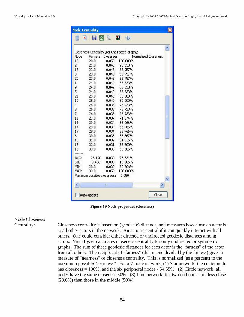
VisuaLyzer User Manual, v.2.0. Copyright 2005-2007 Medical Decision Logic, Inc. All rights reserved.
84
Figure 69 Node properties (closeness)
Node Closeness
Centrality: Closeness centrality is based on (geodesic) distance, and measures how close an actor is
to all other actors in the network. An actor is central if it can quickly interact with all
others. One could consider either directed or undirected geodesic distances among
actors. VisuaLyzer calculates closeness centrality for only undirected or symmetric
graphs. The sum of these geodesic distances for each actor is the "farness" of the actor
from all others. The reciprocal of "farness" (that is one divided by the farness) gives a
measure of "nearness" or closeness centrality. This is normalized (as a percent) to the
maximum possible “nearness”. For a 7-node network, (1) Star network: the center node
has closeness = 100%, and the six peripheral nodes - 54.55%. (2) Circle network: all
nodes have the same closeness 50%. (3) Line network: the two end nodes are less close
(28.6%) than those in the middle (50%).

VisuaLyzer User Manual, v.2.0. Copyright 2005-2007 Medical Decision Logic, Inc. All rights reserved.
85
Figure 70 Node properties (betweenness)
Node Betweenness
Centrality: Betweenness centrality indicates the extent to which an actor falls on the geodesic paths
between other non-adjacent pairs of actors in the network. Betweenness centrality views
an actor as wielding power over interactions between other nodes, to the extent that other
actors depend on it to make connections with other people. For each actor, the
betweenness centrality routine calculates the proportion of times that they are "between"
other actors (e.g., for sending of information) to arrive at a raw score for actor
betweenness centrality. This measure can be normalized by expressing it as a percentage
of the maximum possible betweenness that an actor could have had. The user should
note that calculation of this parameter is a time consuming process as it includes finding
all possible paths between j and k nodes.
Examples for 7 node network: (1). Star network: the center node has betweenness =
100%, and the six peripheral nodes - 0%. (2). Circle network: all nodes have the same
betweenness 20%. (3). Line network: the node in the center of the line (node 4) has
maximum betweenness 60%, the two end nodes have minimum betweenness 0%.
References:
Freeman L C (1979). 'Centrality in Social Networks: Conceptual clarification', Social Networks 1, 215-239.
Borgatti, S.P., Everett, M.G. and Freeman, L.C. 2002. Ucinet 6 for Windows. Harvard: Analytic Technologies.

VisuaLyzer User Manual, v.2.0. Copyright 2005-2007 Medical Decision Logic, Inc. All rights reserved.
86
Nearest neighbor:
The neighborhood of a node i in a graph consists of all nodes adjacent to that node. The nearest neighbor(s)
of a node are those nodes that are closest to it (physically) within a specific distance. To find the nearest
neighbors of a node in VisuaLyzer, follow these steps:
1. Open a graph, and select Nearest Neighbors from the Analysis menu to open the nearest neighbor form,
as in Figure 71.
Figure 71 Nearest neighbors
2. Select a node to find its nearest neighbors (e.g., node 20) in the Krackhardt advice network shown
above.
3. VisuaLyzer returns two groups of nearest neighbors: Group 1 (17 nodes) are within 1 geodesic of node
20. In other words, node 20 and any of these 17 nodes are separated by one geodesic, while the 20
nodes in Group 2 are two geodesics away from node 20.

VisuaLyzer User Manual, v.2.0. Copyright 2005-2007 Medical Decision Logic, Inc. All rights reserved.
87
Shortest Paths
A geodesic is a shortest path. There may be more than one shortest path (or geodesics) connecting any two
nodes. Shortest paths indicate the possible paths that network contents (information, infections, ideas, practices,
etc) can pass efficiently from one node to another and the extent to which this process can be constrained by the
nodes that lie on those paths. The procedure implemented in VisuaLyzer gives the number of all shortest paths
(geodesics) connecting given pair of nodes and provides a way to view all of them, one by one. To find the
shortest paths between any pair of nodes in a graph, follow these steps:
1. Open a graph.
2. Select Shortest Path from the Analysis menu. This will open up the Shortest Path form (Fig. 72) for the
Krackhardt advice network.
3. Select a given pair of nodes, for example, nodes 16 and 14.
4. VisuaLyzer will indicate the number of possible shortest paths found between the two nodes (in this case,
6), and their length (in this case, 2). Each of the six possible paths is listed in the main window of the form,
and the user can use the Select Path control to zoom in to each of the six possible paths, and see their trails
in the graph. Results can be printed or saved in text or excel file formats for further processing.
Figure 72 Shortest path
References:
M. E. J. Newman. "Scientific collaboration networks. II. Shortest paths, weighted networks, and
centrality" Phys. Rev. E 64, 016132 (2001). http://www.santafe.edu/~mark/papers/016132.pdf
VisuaLyzer User Manual, v.2.0. Copyright 2005-2007 Medical Decision Logic, Inc. All rights reserved.
88
Cliques and Clusters (Network Sub-Structures/Sub-Groups)
Sub-structures are important in network analysis because they enable an analyst to gain a micro-view of the
network, showing the various groupings that may be present in a network and the implications of the sub-group
configuration for behavior of members. For example, conflict might be less likely in overlapping cliques
(where some people are members of both cliques) because of shared mutual interests than in non-overlapping
ones, and one might expect diffusion of ideas, practices, and infections to accelerate between such sub-groups
with overlapping memberships. Knowledge about the location of an individual in a sub-group may also be
critical to understanding her/his behavior in the network. For example, while some individuals may act as
"bridges"/"cut-points"/"boundary spanners" between groups, others may have their connections contained
within their own groups, while others may be isolated. Such locational configurations may help the analyst
examine extent to which their embeddedness may facilitate or impede transmission of information and diseases
and diffusion of practices between the subgroups.
Network analysts have developed a number of measures such as cliques (n-cliques, n-clans, and k-plexes)
clusters and partitions that identify the existence of such groups and sub-structures. VisuaLyzer implements
two of these measures: cliques and clusters/partitions
Clique Identification
VisuaLyzer implements the Bron and Kerbosch (1973) algorithm for clique identification. The algorithm
produces basic cliques with overlapping memberships (meaning, nodes can belong to more than one clique). To
generate a clique follow these steps.
1. Open a graph
2. Select Cliques from the Analysis menu,
3. This would open up a clique configuration panel as well as the graph showing the default cliques
containing tree or more members (by default, VisuaLyzer produces cliques with at least 3 members).
4. You can change the minimum size of the clique, using the configuration panel, and you can select a
particular clique (clique 1, 2, 3 etc.) at a time for closer inspection.
5. Once you select a particular clique membership, you can apply a number of attributes (shape, color and
size) to visually distinguish them.
6. For example, Figure 73 shows cliques (minimum size = 5) for Krackhardt‟s High-Tech managers advice
network. The graph shows clique 1 (with green colored, diamond shaped-nodes).

VisuaLyzer User Manual, v.2.0. Copyright 2005-2007 Medical Decision Logic, Inc. All rights reserved.
89
Figure 73 Cliques
Clusters and Communities:
VisuaLyzer implements the Newman and Girvan algorithm for finding clusters/communities in graphs (see
references below). The algorithm is based on the idea of modularity. Given any network, the clustering
algorithm always produces some division of the nodes into communities, regardless of whether the network has
any natural such division.
To test whether a particular division is meaningful the algorithm defines quality function or “modularity” Q as
follows. Let Eij be the fraction of edges in the network that connect nodes in group i to those in group j, and let
Ai = Sum(Eij). Then Q = Sum(Eii – Ai^2). Thus, the modularity is the fraction of the edges in the network that
connect nodes within community minus the expected value of the same quantity in a network with the same
community divisions but random connections between the nodes. If the number of within-community edges is
no better than random, we will get Q = 0. Values approaching Q = 1, which is the maximum, indicate strong
community structure. In practice, values for such networks typically fall in the range from about 0.3 to 0.7.
Higher values are rare.
The algorithm falls in the general category of agglomerative clustering methods. It assumes that graphs are
undirected with unweighted edges. Starting with a state in which each node is the sole member of one of N
Clique Configuration Panel

VisuaLyzer User Manual, v.2.0. Copyright 2005-2007 Medical Decision Logic, Inc. All rights reserved.
90
clusters, we repeatedly join clusters together in pairs, choosing at each step the join that results in the greatest
increase (or smallest decrease) in quality function, or modularity Q. The worst-case running time of the
algorithm is O((M + N)N), or O(N^2) on a sparse graph, where M is number of links and N is number of nodes
in the network. The algorithm has the added advantage of calculating the value of Q as it goes along, making it
especially simple to find the optimal community structure: we select the best partotion of the network by
looking for the largest value of Q.
Finding clusters
To implement clustering algorithm:
1. Open a graph (e.g., Krackhardt‟s Advice relation is used in this case)
2. Select Analysis > Partitions/Clusters > Clustering menu. This will perform a hierarchical clustering
procedure on the graph:
Figure 74 Clusters
The main output of the procedure is a Partitions/clusters form which lists membership for each cluster.

VisuaLyzer User Manual, v.2.0. Copyright 2005-2007 Medical Decision Logic, Inc. All rights reserved.
91
3. The Number of clusters option on the form can be used to instruct VisuaLyzer to select a particular
number of clusters in the graph. For example, in Figure 74, VisuaLyzer displays 3 clusters for the
advice relation graph.
4. Additionally, the Select cluster # can be used to select all members of a particular cluster. Upon
selection, the user can apply different attributes (color, size shape) to all cluster members to distinguish
them from the other clusters, as the example above shows. In addition, a cluster number is printed at the
edge of each cluster, to further distinguish the clusters.
5. Contents of the Partition/Clusters form can be saved, printed or exported to Excel for further optional
processing.
Finding Communities:
As stated above, this algorithm divides a network graph in to various communities or components that may be
in existence in the natural community. The fit of the implementation is examined through the modularity (Q)
index – the higher the value, the closer the divisions approximate those occurring in the natural community.
Figure 75 Communities

VisuaLyzer User Manual, v.2.0. Copyright 2005-2007 Medical Decision Logic, Inc. All rights reserved.
92
To divide a graph into communities:
1. Open a graph.
2. Select Analysis > Partitions/clusters > Optimal Partition (Communities) menu as it is shown in Figure
75.
3. The Communities form displays the name of the relation, number of communities in the graph (a
message box will indicate if no communities are found), the modularity index (Q), as well as options for
the user to cycle through and select each of the community members for closer examination, or editing
(change color, size and shape).
4. The example above implements the algorithm on Krackhart‟s REPORTS_TO relation (a component of
the High Tech Managers study). A closer examination of the data gives a sense of natural divisions,
based on departmental affiliation, tenure, and to some extent seniority level. The algorithm produces
two communities; the high modularity index indicates a good fit to the data.
5. The algorithm as well as knowledge of the organization may provide further strength and validation of
this observation. This implementation would be most useful when applied to large networks, which
may, a priori, have some internal divisions.
References:
Borgatti, S.P., Everett, M.G. and Freeman, L.C. 2002. Ucinet 6 for Windows. Harvard: Analytic
Technologies.
Johnson, S C (1967). 'Hierarchical clustering schemes'. Psychometrika, 32, 241-253.
M. E. J. Newman. Detecting community structure in networks. In Eur. Phys. J. B., 2004. http://www-
personal.umich.edu/~mejn/papers/epjb.pdf
M. E. J. Newman and M. Girvan, Finding and evaluating community structure in networks, Physical
Review E 69, 026113 (2004). http://arxiv.org/PS_cache/cond-mat/pdf/0308/0308217.pdf
M. E. J. Newman. Fast Algorithm for Detecting Community Structure in Networks. Physical Review E
69, 066133 (2004). http://aps.arxiv.org/PS_cache/cond-mat/pdf/0309/0309508.pdf

VisuaLyzer User Manual, v.2.0. Copyright 2005-2007 Medical Decision Logic, Inc. All rights reserved.
93
Roles and Positions
In social network analysis, the concept of position refers to a collection of individuals who are similarly
embedded in network of relations, while role refers to the pattern of relations between positions. Actors in a
same position have similar patterns of relations and interactions with other actors. “Similar relations” doesn‟t
necessarily mean “directly connected”, though. For example, students in different schools have similar
relations with teachers and parents. They occupy the position of “student” and perform a specific role, though
individual students may not know each other. Thus, position and role is a measure of structural equivalence
rather than adjacency or connectedness.
Structurally equivalent actors have the same profile except for the diagonal entries of the adjacency matrix.
Role and position algorithms often take as their input a similarity or distance matrix. Some common measures
of similarity and dissimilarity are: Euclidean Distance and Pearson Correlation. VisuaLyzer implements a
single-link hierarchical clustering, using Euclidean distance as a measure of dissimilarity. Starting with a state
in which each node is the sole member of one of N clusters, it repeatedly joins clusters together in pairs,
choosing at each step the actor that is closer to others by his/her position in the network. The running time of
the algorithm is O(N^2).
Performing role and positional analysis involves the following steps:
1. Preparing the data prior to analysis (e.g., calculation of similarity and dissimilarities, scaling, if any)
2. Selecting a similarity or dissimilarity measure which gauges the extent to which two actors approach
structural equivalence or substitutability
3. Clustering the similarity/dissimilarity measures from step 2, and selecting a cluster or partitioning of the
actors into positions
4. Superimposing the partition from step 3 on the basic input data, and examining the positional or sub-
group density matrices to help interpret the relationship between and within the subgroups/positions
5. Dichotomize the entries in the subgroup density matrices (by using an alpha threshold) to create a binary
image matrix that indicates the presence or absence of positional relations.
To run the Roles and Positions procedure, follow these steps:
1. Open a graph.
a. Note: Any single graph with unweighted edges is supported in the current version of VisuaLyzer.
Future versions will support multiple and valued relations.
b. VisuaLyzer will symmetrize the graph automatically (using the maximum procedure, if the graph
is directed), and will transform it into dissimilarities before submitting it to the roles and
positions procedure for partitioning into discrete positions.
2. Select Analysis > Roles and Positions from the menu. This will return the positional profile on the graph
(Fig. 76).
3. The Number of positions box on the Roles and Partitions form allows the user to select a number of
positions of interest. The example below selects three positions for the Krackhardt‟s advice network.
4. Managers in each of these positions are structurally equivalent. Membership of each of these positions
can be interpreted based on knowledge of the network, and attributes of individual nodes. For example,
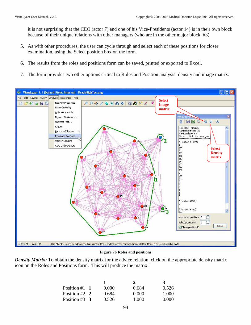
VisuaLyzer User Manual, v.2.0. Copyright 2005-2007 Medical Decision Logic, Inc. All rights reserved.
94
it is not surprising that the CEO (actor 7) and one of his Vice-Presidents (actor 14) is in their own block
because of their unique relations with other managers (who are in the other major block, #3)
5. As with other procedures, the user can cycle through and select each of these positions for closer
examination, using the Select position box on the form.
6. The results from the roles and positions form can be saved, printed or exported to Excel.
7. The form provides two other options critical to Roles and Position analysis: density and image matrix.
Figure 76 Roles and positions
Density Matrix: To obtain the density matrix for the advice relation, click on the appropriate density matrix
icon on the Roles and Positions form. This will produce the matrix:
1 2 3
Position #1 1 0.000 0.684 0.526
Position #2 2 0.684 0.000 1.000
Position #3 3 0.526 1.000 0.000
Select
Density
matrix
Select
Image
matrix

VisuaLyzer User Manual, v.2.0. Copyright 2005-2007 Medical Decision Logic, Inc. All rights reserved.
95
a. The entry in the density matrix is the proportion of links that are present between the cluster in
the row position and the cluster in the column position. For example, the entry 0.684 indicates
that almost 70% of links between positions 1 and 2 are in existence, showing dense
interconnectivity between the positions.
b. Image Matrix: To obtain the image matrix for the advice relation, click on the appropriate image
matrix icon on the Roles and Positions form. This will produce the matrix:
1 2 3
Position #1 1 0 1 1
Position #2 2 1 0 1
Position #3 3 1 1 0
c. The cell entries indicate the presence (1) or absence (0) of relations between the various
positions or blocks. Indicating the presence or absence of relation is based on setting a threshold
or cut-off value for the density matrix. Cell entries that exceed the cut-off value indicate the
presence of a relation between the positions, and zero otherwise. Traditionally, researchers have
used the overall density (alpha density) of the relation/matrix as a cut-off value. VisuaLyzer
implements a rather simple cut off value of (0), indicating any density value above (0) as
indicating the presence of relations. This may over-estimate the presence of relations between
positions, and future versions of VisuaLyzer will allow the user to select a different threshold
value to create the image matrix.
References:
S. Wasserman and K. Faust. Social network analysis. Methods and Applications. Cambridge University
Press, Cambridge, 1994.
Burt R (1976). Positions in Networks. Social Forces, 55, 93-122.
Cutpoints
In social network analysis, cutpoint (or 1-node cutset) is a node whose deletion would increase the number of
components in a graph. The graph may contain many, just one cutpoint, or even no cutpoints at all (consider a
circle: two nodes have to be removed to disconnect the graph). VisuaLyzer recognizes isolated nodes, dyads,
and components of size 3 and more. These components are one of the results of partition/cluster analysis. So to
find cutpoints VisuaLyzer runs partition/cluster analysis for virtual removal of each graph node and compares
the total number of components before and after the removal. As always, disabled nodes, as well as isolates and
nodes with degree centrality of 1 are excluded from the calculations.
Size of components created by the removal of a cutpoint varies from just one node to the half of the graph. To
estimate the degree of graph fragmentation after cutpoint removal we use two measures: absolute and relative
disintegrations. Assuming there is 100% disintegration if we get all N nodes of the graph disconnected, absolute
disintegration will be (TotalComp-1)/(N-1). If the component count is 1, there is no fragmentation. Relative
disintegration is defined as a ratio of total component numbers after/before cutpoint removal. We leave the final
decision about an importance of each particular cutpoint to the user.

VisuaLyzer User Manual, v.2.0. Copyright 2005-2007 Medical Decision Logic, Inc. All rights reserved.
96
To run the Roles and Positions procedure, follow these steps:
1. Open a graph.
a. Note: Any single graph with unweighted edges is supported in the current version of VisuaLyzer.
Future versions will support multiple and valued relations.
b. VisuaLyzer will symmetrize the graph automatically (using the maximum procedure, if the graph
is directed), and will transform it into dissimilarities before submitting it to the cutpoint
procedure.
2. Select Analysis >Cutpoints from the menu. This will return the positional graph with selected cutpoint
nodes if any are found (two nodes have been identified in Fig. 77).
3. The results from the Cutpoints form can be saved, printed or exported to Excel.
Figure 77 Cutpoints
References:
S. Wasserman and K. Faust. Social network analysis. Methods and Applications. Cambridge University
Press, Cambridge, 1994.

VisuaLyzer User Manual, v.2.0. Copyright 2005-2007 Medical Decision Logic, Inc. All rights reserved.
97
Opinion Leaders
Over the past 50 years, theories on diffusion of innovations have been used to study the spread of new ideas,
information and practices in a variety of applied settings. Opinion leaders have been recognized as critical
elements in the diffusion process, largely because of their ability to reach and diffuse
ideas/information/practices to their followers. Among the techniques used to select opinion leaders, sociometric
techniques have assumed a central place given their utilization of interpersonal communication patterns of
leaders and their followers.
VisuaLyzer implements one technique - a matching algorithm developed by T. Valente (1996, 1990) to select
opinion leaders and match them to their followers. The algorithm assumes directed relations. It attempts to:
Find out who are the Opinion Leaders, and
Assign (match) the rest of the network to the leaders optimally, creating groups of approximately the
same size.
A detailed discussion of the algorithm and its assumptions are presented in the Algorithm Implementation
section below.
To run the Opinion Leaders procedure, follow these steps:
1. Open a directed graph). The graph used in this example can be found at
\Examples\Binary\OpinionLeaders.eng in the installation folder.
2. Select Analysis > Opinion Leaders from the menu. This will first present the user with a pop-up
message box requesting the desired number of opinion leaders to derive, up to the maximum detected
and suggested by the program:
Figure 78 Selecting number of leaders
3. Select the number of opinion leaders desired and click OK button. This will return a new graph with the
socio-metrically derived opinion leaders selected (Fig. 79).
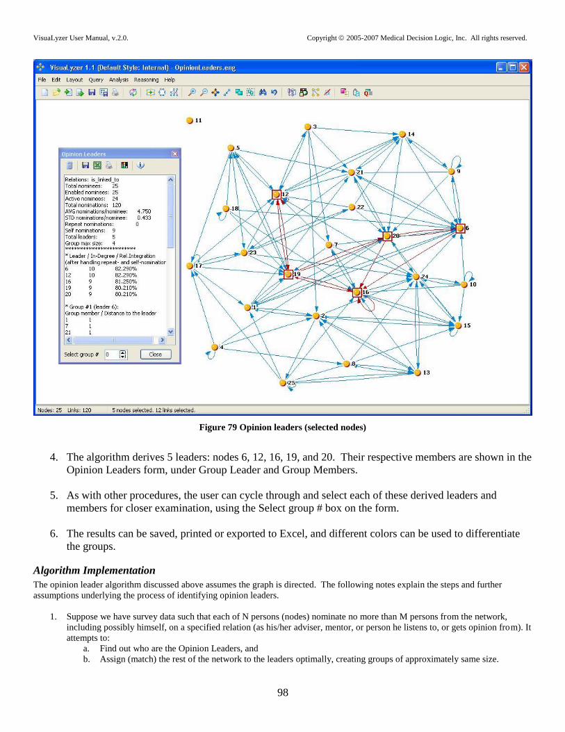
VisuaLyzer User Manual, v.2.0. Copyright 2005-2007 Medical Decision Logic, Inc. All rights reserved.
98
Figure 79 Opinion leaders (selected nodes)
4. The algorithm derives 5 leaders: nodes 6, 12, 16, 19, and 20. Their respective members are shown in the
Opinion Leaders form, under Group Leader and Group Members.
5. As with other procedures, the user can cycle through and select each of these derived leaders and
members for closer examination, using the Select group # box on the form.
6. The results can be saved, printed or exported to Excel, and different colors can be used to differentiate
the groups.
Algorithm Implementation
The opinion leader algorithm discussed above assumes the graph is directed. The following notes explain the steps and further
assumptions underlying the process of identifying opinion leaders.
1. Suppose we have survey data such that each of N persons (nodes) nominate no more than M persons from the network,
including possibly himself, on a specified relation (as his/her adviser, mentor, or person he listens to, or gets opinion from). It
attempts to:
a. Find out who are the Opinion Leaders, and
b. Assign (match) the rest of the network to the leaders optimally, creating groups of approximately same size.

VisuaLyzer User Manual, v.2.0. Copyright 2005-2007 Medical Decision Logic, Inc. All rights reserved.
99
2. The number of leaders is derived from the pattern of nominations (out-degrees) in the network. If the SD/AVERAGE ratio
for the number of nominations per nominee is relatively small (less that 0.67 in our case), the program assumes there are
M=round (AVERAGE) maximum number of leaders in the network and suggests this number to the user to choose the exact
number (<= M) that is desired.
3. If the ratio is big (more than .67), the program can theoretically assign 10% of the network membership as leaders (the
assumption is that 10% would be convenient for most settings and applications). Passive nominees (nodes with out-
degree=0) are excluded from the calculation of the ratio.
4. To find out the M opinion leaders, the program compares the in-degree of the persons. If in-degrees are the same, it further
compares the relative integration (Valente, 1998) of the candidates. The integration criterion shows the degree to which an
individual's inward nominations integrate him/her into the network. The integration is a centrality measure that is based on
the so called inverse Guimares Relative Integration Index, or reverse distance matrix calculations (cited in Valente, 1998).
The M leaders then are matched to the N-M persons in the community who nominated them.
5. We assume the size of group for each leader is approximately the same: (N-M)/M. If someone did not directly nominate a
leader, that person is matched to a leader who is closest (by distance) to him/her. If he is equally close to two or more
leaders, then indirect paths are used to determine optimal pairing (geodesic distance=2). During data processing the
procedure ignores repeated nominations, i.e. when a person nominated other person more than once; it also ignores self-
nominations.
6. If weights or values are assigned to links, for example when users are asked to list important nodes first, followed by less
important ones, the first nominee is assigned a value of 1, the next 2, and the last …N. In such a case, selection of group
members will reflect the nomination ranks.
Note: The lower the weight (e.g. the case of weight 1), the higher is the rank of the nominee and such a nominee
will be listed first as a member of the group.
Note: If all links to nominees have the same weight or are even unweighted (as in the example above), then group
members are selected based on previous criteria only (point #5 above).
7. The output of the Opinion Leaders procedure is the list of leaders and list of group members for each leader together with
additional parameters showing selection reason and sorting order.
References:
Thomas W. Valente, Rebecca L. Davis. Accelerating the Diffusion of Innovations Using Opinion
Leaders. ANNALS, AAPSS, 566, November 1999.
Thomas W. Valente. Social Network Thresholds in the Diffusion of Innovations. Social Networks 18:
69 – 79
Thomas W. Valente, Robert K. Foreman. Integration and Radiality: Measuring The Extent Of an
Individual's Connectedness And Reachability in a Network. Social Networks 20 (1998) 89-105
Thomas W. Valente. cctrial_kv4.prg - a GAUSS program that finds opinion leaders and assigns them
leaders to groups.

VisuaLyzer User Manual, v.2.0. Copyright 2005-2007 Medical Decision Logic, Inc. All rights reserved.
100
1 2 3 4 5 6 7 1 1 1 | . . . .
2 1 1 | . . . .
3 1 1 | . . . .
- - - - | - - - -
4 . . . | 0 0 0
5 . . . | 0 0 0
6 . . . | 0 0 0
7 . . . | 0 0 0
Core and Periphery
Core-periphery analysis is central in network analysis because it offers interesting insights into social
stratification. Who are the core actors of the network? Who the peripheral? Intuitively, core nodes are
connected to each other more or in many more ways than with other nodes, whereas peripheral nodes have
weak connections with each other and with other nodes.
Ideal core/periphery structure can be discrete or continuous. Discrete models produce two distinct classes of
nodes: those of the core nodes that have relations with each other alone and those on the periphery. The
continuous model assigns nodes to different degrees of “coreness” - a sort of a continuous measure.
VisuaLyzer implements a discrete model discussed by Borgatti (1999). In this model, the core/periphery
analysis algorithm seeks a partition that maximizes density in the core and minimizes the density in the
periphery. Ties between these two regions are ignored in the computation. A simple example of a symmetric
adjacency matrix for an ideal structure is shown below:
In this case the nodes 1, 2 and 3 are core nodes. Note, that because of ignoring
some ties, many networks satisfying this model will have the same core and
periphery.
VisuaLyzer implements the Kernighan-Lin algorithm that is proven to be fast and able to search global
optimal core/periphery structure, see Boyd (2004). Boyd's description of the algorithm is provided
below under Kernighan-Lin algorithm.
The algorithm begins by permuting the rows and columns of the adjacency matrix and comparing the
results with some corresponding "ideal" matrix on each step. It computes a measure of "fitness" that
indicates how well the observed clusters approximate an ideal core/periphery structure. This measure of
fitness is similar to the Pearson Correlation Coefficient UCINET uses to judge the adequacy of the
observed core-periphery pattern with the idealized pattern.
The current version of VisuaLyzer uses a simple matching coefficient for matrices A and B instead to
reduce the computation time. The coefficient is expressed as:
r = SUMiSUMj( f(Aij, Bij) ), where the function f(Aij, Bij) returns 1 (0) when Aij=Bij (Aij<>Bij) for
both core and periphery regions of the matrix. If the region's data are totally opposite to the model then
r=0, if they are identical r=1.
Normalization only includes the sum of nodes in the regions. Diagonals, self-loops and disabled nodes
are excluded from the analysis.
The Core and Periphery procedure produces two lists of nodes - for core and periphery - and normalized
correlation coefficient r (named "core centralization") that shows how well the real structure
approximates the corresponding model.

VisuaLyzer User Manual, v.2.0. Copyright 2005-2007 Medical Decision Logic, Inc. All rights reserved.
101
The core centralization coefficient r is constrained to the range between -1 to +1 to be comparable with
the measurements based on Pearson's coefficient. Cases with r >= 0.9 are marked as "perfect fit", cases
r < 0.1 (and < 0) are marked as "no fit".
To detect a core-periphery structure in a network, follow these steps:
1. Open a network graph. The graph used in this example can be found at ..\Examples\Binary\
KrackHighTec.eng in the installation folder.
2. Select Analysis > Core and Periphery from the menu. This will present a new graph, partitioning the
network into core and peripheral nodes (Fig. 80).
3. The user can select the core or peripheral nodes by the clicking on the corresponding Show buttons on
the Core-Periphery form. Once selected, the user can apply color, shape and other visual properties to
distinguish between the two kinds of nodes.
4. The associated Core & Periphery form presents detailed results of the analysis procedure.
Total and Enabled Nodes: This shows that there are 21 nodes in the data and all are enabled
(available for analysis)
Core Nodes: Number of nodes in the core
Periphery Nodes: Number of nodes in the periphery
Core-Periphery Ratio: The number of Core Nodes divided by the number of Peripheral Nodes.
Core Centralization: An indicator of fit to the ideal model. The higher the coefficient (closer to 1),
the better the fit is to the ideal model.
5. The results from the Core and Periphery form can be saved, printed or exported to Excel.
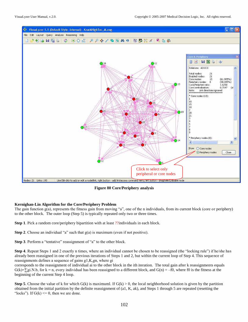
VisuaLyzer User Manual, v.2.0. Copyright 2005-2007 Medical Decision Logic, Inc. All rights reserved.
102
Figure 80 Core/Periphery analysis
Kernighan-Lin Algorithm for the Core/Periphery Problem
The gain function g(a), represents the fitness gain from moving “a”, one of the n individuals, from its current block (core or periphery)
to the other block. The outer loop (Step 5) is typically repeated only two or three times.
Step 1. Pick a random core/periphery bipartition with at least ??individuals in each block.
Step 2. Choose an individual “a” such that g(a) is maximum (even if not positive).
Step 3. Perform a “tentative” reassignment of “a” to the other block.
Step 4. Repeat Steps 1 and 2 exactly n times, where an individual cannot be chosen to be reassigned (the “locking rule”) if he/she has
already been reassigned in one of the previous iterations of Steps 1 and 2, but within the current loop of Step 4. This sequence of
reassignments defines a sequence of gains g1,Κ,gn, where gi
corresponds to the reassignment of individual ai to the other block in the ith iteration. The total gain after k reassignments equals
G(k)=∑gi.N.b, for k = n, every individual has been reassigned to a different block, and G(n) = –f0, where f0 is the fitness at the
beginning of the current Step 4 loop.
Step 5. Choose the value of k for which G(k) is maximuml. If G(k) > 0, the local neighborhood solution is given by the partition
obtained from the initial partition by the definite reassignment of (a1, K, ak), and Steps 1 through 5 are repeated (resetting the
“locks”). If G(k) <= 0, then we are done.
Click to select only
peripheral or core nodes

VisuaLyzer User Manual, v.2.0. Copyright 2005-2007 Medical Decision Logic, Inc. All rights reserved.
103
References:
Borgatti, S.P., Everett, M.G, 1999. Models of Core/Periphery structures. Social Networks 21, 375-395
http://www.analytictech.com/borgatti/cp_structure.doc
John P. Boyd, William J. Fitzgerald, and Robert J. Beck. Computing Core/Periphery Structures and Permutation Tests
for Social Relations Data (September 28, 2004). Institute for Mathematical Behavioral Sciences. Paper 16.
http://hypatia.ss.uci.edu/imbs/tr/mbs04_13.pdf

VisuaLyzer User Manual, v.2.0. Copyright 2005-2007 Medical Decision Logic, Inc. All rights reserved.
104
FORMAL REASONING ABOUT SOCIAL NETWORK DATA
Links as Facts
The viewpoint taken in this section is a little different. Many approaches to network analysis take as
fundamental either an adjacency matrix or an edgelist. Additionally, the network editing portion of VisuaLyzer
assumes that the network drawn is the founding knowledge. In this section, sentences as facts are fundamental
and networks or matrices are derived from the stated facts, at least conceptually. From these facts we can set up
equations on relations and solve for network unknowns using the axioms of a relation algebra.
Statements of fact are simple sentences of the form Subject verb Object. Predicates (verbs) relate a source
Subject with a sink Object. Directed edges in a network can also depict these sentences. The predicate is the
relation that names a set of directed edges. The nodes are the subjects and objects. Such simple sentences are
assertions of what is known and true; a missing or unasserted sentence is assumed to be false. Then the model
is explicitly available for criticism as to how complete or consistent it is. The logical operations do not directly
apply to the „real‟ world. Instead, they apply very strongly and very precisely to this model of the real world.
Boolean operations
Boolean algebras are more general than relation algebras because there are fewer values and fewer operations
involved. In the simple Boolean logical systems there are only TRUE and FALSE values. In the binary
systems at the foundations of digital computing, there are only 0 and 1 bits. Also, there are three basic
operations (Boolean functions): AND, OR, and NOT. Truth tables give precise meanings for these operations:
A B A AND B A B A O R B
0 0 0 0 0 0
0 1 0 0 1 1
1 0 0 1 0 1
1 1 1 1 1 1
In a digital circuit, 0 may represent an open switch and 1 a closed switch. In the circuit made of the AND gate,
current can flow only if both switches A and B are closed. The expression A*B represents the corresponding
product (intersection) of sets. In the circuit made of the OR gate, current can flow if at least one of A or B is
closed. The expression A+B represents the corresponding sum (union) of sets. Similarly, the conjunction of
two sentences A AND B is true only if both sentences A and B are each true; the disjunction of two sentences A
OR B is true only if A is true or if B is true or they are both true. As should be apparent, there are
isomorphisms between logic, set theory, and digital circuit.
Although AND and OR are fundamental they are not enough as primitives for Boolean logic. The additional
operation, NOT, negates any value to its opposite. The following truth table shows the outputs of NOT from its
inputs:

VisuaLyzer User Manual, v.2.0. Copyright 2005-2007 Medical Decision Logic, Inc. All rights reserved.
105
A NOT A
0 1
1 0
As one would expect, the NOT Boolean function maps sentences that are TRUE or FALSE into corresponding
sentences that are FALSE or TRUE. Similarly, the set complement maps empty and universal sets into
universal and empty sets. The notation for the complement function on a set S is complement(S).
It is straightforward to extend these concepts to sets of more than one element. These larger sets correspond to
an extension of the bit operations to more than one bit, to words of bits. This, in turn, corresponds to an
arrangement of switches in a parallel circuit. As an example, consider the subset {a,c,d} of the set {a,b,c,d}.
This could be represented as a 4-bit word as 1011 where the left to right position of the bits correspond in
alphabetic order to the letters a,b,c,d. Similarly, this can match with 4 independent switches that are, in turn,
closed, open, closed, and closed.
Relations are sets as well - sets of ordered pairs. Bits 0 and 1 can still indicate presence or absence of a link and
sequenced into a word, as before, to represent a set of links, a relation. Now a closed switch in a digital circuit
can link two junctures (two nodes); when the switch is open, the link is absent. The set of edges in a network is
a relation but some relations do not have a network representation. For example, the subset of edges in a
network consisting of self loops is a subset of the identity relation. Everything else (the complement of the
identity) is the apartness relation that even relates nodes that are not necessarily in the original network. The
identity and apartness relations are infinite but implemented finitely as constraints.
Finally, the nodes of the network themselves can have a deeper „term‟ structure. In the reasoning part of
VisuaLyzer, the universe is limited to terms. A term is a constant or variable (NA) or a complex term. A
complex term is a function symbol, f (a constant) followed by a parentheses enclosed, comma separated, list of
terms of the form f(t1,t2,…,tn). Terms themselves have a representation as a rooted, directed, ordered, acyclic
network.
With relations come concepts of query and computation. We can define new relations as expressions
combining other relations and operators. Not only can we test for membership in a relation but we can query
for the members as pairs or provide one object and query for the other.
The underlying model is a collection of sets of ordered pairs of terms – a collection of networks of networks –
and unifies high level software with the underlying low level hardware circuitry.
Relation operations
The knowledge base consisting of a collection of facts and displayed as directed networks, is a sub theory of the
theory of relations. Relations are sets of ordered pairs and operations on them satisfy the rules of classical set
theory, specifically both Boolean and relation algebras. The basic operations on relations are
1) absolute sum or union of relations R and S is R+S = {x:y|x R y or x S y}.
2) absolute product or intersection of relations R and S is R*S = {x:y| x R y and x S y}.
3) relative product (composition) of relations R and S is R:S = {x:y | there exists z, x R z and z S y}.
4) the complement of the relation R, those pairs not in R, is complement(R) = {x:y | x R y is not true}.

VisuaLyzer User Manual, v.2.0. Copyright 2005-2007 Medical Decision Logic, Inc. All rights reserved.
106
5) the converse of the relation R is converse(R) = {x:y| y R x}.
6) the identity relation (relative unit), which is the set of pairs {x:y|x=y}, is id.
7) a selector p^n-j, is the set {x:y|for every x1,x2,…xn, x=p(x1,x2,…,xj-1,y,xj+1,…,xn}.
These operations are available within the Reasoning -> Arbitrary Relations -> Relation Combinators menu.
Note the hints at the bottom of the display.
An individual selector and any expressions involving inequalities are not depicted in VisuaLyzer as a network
but as a set expression. Generally, every set of directed edges (ordered pairs) is a relation, but a relation is not
necessarily a set of directed edges. The identity relation could be envisioned as a set of self loops on an infinite
set of nodes and depicted as a single self loop on a node with a name as variable or not available (NA). Even if
R is a finite set of edges, the constructive complement(R) is an infinite set; complement(R) can always be
finitely described as a collection of (perhaps existentially quantified) equations and (universally quantified)
inequations in disjunctive normal form. Thus, complement(R) differs from the graph complement. The relation
complement represents the negation of all the knowledge in the relation. The graph complement is the set of
edges that are not in the original network. For a network, g, the graph complement is
complete(g)*complement(g) if complete(g) is the complete graph containing g.
These primitives can help define other primitives. The apartness relation di (relative zero or diversity), is
complement(id). Absolute unit, 1, is id+di and zero, 0, is id*di. The relative sum, R&S, is
complement(complement(R):complement(S)). Finally, an explicitly defined set is a brace delimited, comma
separated collection of pairs that are each colon separated – such as, {ann:carl, carl:bill}. In an infinite
universe, the complement of that finite set would be infinite. However, complement({ann:carl, carl:bill}) has a
finite description as a collection of equations and inequations in disjunctive normal form:
{x:y| x=ann ^ y != carl
V x=carl ^ y!= bill
V x !=ann ^ x!=carl}.
This constructive complement satisfies the usual properties of Boolean algebra (and relation algebra). If a set
description uses an existentially quantified variable in an equation, its complement would require a universal
quantified variable in the corresponding inequations. For example, complement(p^3-1) = {NAx:NAy|
for_every(NA1,NA2)(NAx != p(NAy,NA2,NA1))} where, in such a set description, for_every(NA1,NA2) means
that NA1 and NA2 are universally (for all) quantified. As expected of a classical complement, it is particularly
true that complement(complement(p^3-1))=p^3-1.
Variables in VisuaLyzer are a hybrid of the traditional notion of a value that is Not Available (NA) and the
mathematical symbols x and y. A variable name is chosen by the following rules: 1) it consists of the two
characters NA in any case mixtures, or 2) it begins with NA in any mixture of case, and is followed by any
number of characters, the first of which is chosen from 0..9,x,y,z. Both node names and attribute values may be
NA (Not Available). If nodes have no attributes then their names represent them. If nodes have attributes then
they have a deeper term structure of the form
node(name(NameValue),attribute1(Value1),…attributeN(ValueN)).
The relation operations form a highly symmetric arrangement and comprise the operations of a structure
described in Tarski & Givant as a representable relation algebra (RRA):
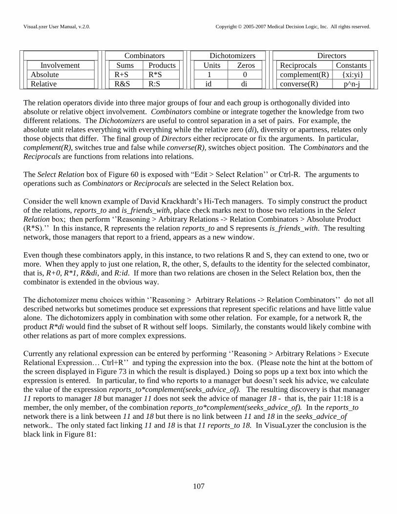
VisuaLyzer User Manual, v.2.0. Copyright 2005-2007 Medical Decision Logic, Inc. All rights reserved.
107
Involvement
Absolute
Relative
Combinators
Sums Products
R+S R*S
R&S R:S
Dichotomizers
Units Zeros
1 0
id di
Directors
Reciprocals Constants
complement(R) {xi:yi}
converse(R) p^n-j
The relation operators divide into three major groups of four and each group is orthogonally divided into
absolute or relative object involvement. Combinators combine or integrate together the knowledge from two
different relations. The Dichotomizers are useful to control separation in a set of pairs. For example, the
absolute unit relates everything with everything while the relative zero (di), diversity or apartness, relates only
those objects that differ. The final group of Directors either reciprocate or fix the arguments. In particular,
complement(R), switches true and false while converse(R), switches object position. The Combinators and the
Reciprocals are functions from relations into relations.
The Select Relation box of Figure 60 is exposed with “Edit > Select Relation‟‟ or Ctrl-R. The arguments to
operations such as Combinators or Reciprocals are selected in the Select Relation box.
Consider the well known example of David Krackhardt‟s Hi-Tech managers. To simply construct the product
of the relations, reports_to and is_friends_with, place check marks next to those two relations in the Select
Relation box; then perform „‟Reasoning > Arbitrary Relations -> Relation Combinators > Absolute Product
(R*S).‟‟ In this instance, R represents the relation reports_to and S represents is_friends_with. The resulting
network, those managers that report to a friend, appears as a new window.
Even though these combinators apply, in this instance, to two relations R and S, they can extend to one, two or
more. When they apply to just one relation, R, the other, S, defaults to the identity for the selected combinator,
that is, R+0, R*1, R&di, and R:id. If more than two relations are chosen in the Select Relation box, then the
combinator is extended in the obvious way.
The dichotomizer menu choices within „‟Reasoning > Arbitrary Relations -> Relation Combinators‟‟ do not all
described networks but sometimes produce set expressions that represent specific relations and have little value
alone. The dichotomizers apply in combination with some other relation. For example, for a network R, the
product R*di would find the subset of R without self loops. Similarly, the constants would likely combine with
other relations as part of more complex expressions.
Currently any relational expression can be entered by performing „‟Reasoning > Arbitrary Relations > Execute
Relational Expression… Ctrl+R‟‟ and typing the expression into the box. (Please note the hint at the bottom of
the screen displayed in Figure 73 in which the result is displayed.) Doing so pops up a text box into which the
expression is entered. In particular, to find who reports to a manager but doesn‟t seek his advice, we calculate
the value of the expression reports_to*complement(seeks_advice_of). The resulting discovery is that manager
11 reports to manager 18 but manager 11 does not seek the advice of manager 18 - that is, the pair 11:18 is a
member, the only member, of the combination reports_to*complement(seeks_advice_of). In the reports_to
network there is a link between 11 and 18 but there is no link between 11 and 18 in the seeks_advice_of
network.. The only stated fact linking 11 and 18 is that 11 reports_to 18. In VisuaLyzer the conclusion is the
black link in Figure 81:

VisuaLyzer User Manual, v.2.0. Copyright 2005-2007 Medical Decision Logic, Inc. All rights reserved.
108
Figure 81 Determine who reports to, but does not seek the advice of, which manager.
There is only one edge (only two nodes) in the reports_to*complement(seeks_advice_of) relation. In this case it
is true that 11 reports to 18 but not true that 11 seeks the advice of 18. Note that if animation is turned off, then
the new link (the new relation, reports_to*complement(seeks_advice_of), is drawn without disturbing the
original relation, reports_to. This is done with F4 (General properties) -> General -> uncheck Animation.
Variables
The relative product {ann:bill}:1 has a set description which requires the use of variables. As a set it is {x:y|
x=ann}; the variable y can have any value as it is unconstrained. In VisuaLyzer, this would be depicted as a
single link from a node named ann to a node named NA (Not Available). In general, a node named NA can have
any number of valid values for each single depiction.
As another example, consider {ann:bill}:di which is the set {x:y|x=ann ^ y \= bill}. In this example, y can again
take on a number of values – everyone but bill. This set is not depicted in VisuaLyzer as a network, as
attributes in VisuaLyzer can only be positive, equality constraints. Instead, this is displayed in another window
as a set description.
Other representation examples based on the knowledge encoded in the relations is_friends_with,
seeks_advice_of, and reports_to follow. The italicized words, e.g. Friend, Advisor, Someone, Who and Whom,
replace the object variables x and y in the corresponding set expression.
1. Who seeks advice from which Friends?
seeks_advice_of*is_friends_with.
2. Who seeks advice from which Friends that are also supervisors?
seeks_advice_of*is_friends_with*reports_to
3. Who has Friends_of_friends that are not friends (i.e. Who are Candidates for introduction?)
(is_friends_with:is_friends_with)*complement(is_friends_with)*di.
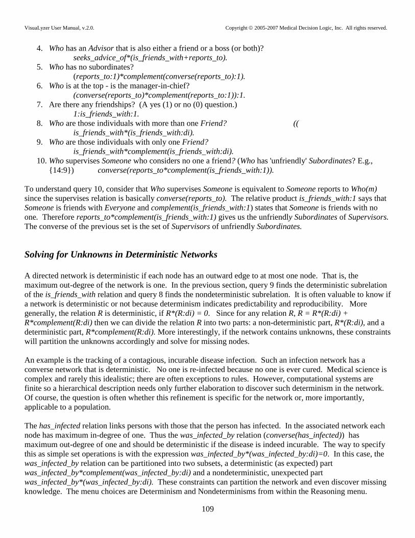
VisuaLyzer User Manual, v.2.0. Copyright 2005-2007 Medical Decision Logic, Inc. All rights reserved.
109
4. Who has an Advisor that is also either a friend or a boss (or both)?
seeks_advice_of*(is_friends_with+reports_to).
5. Who has no subordinates?
(reports_to:1)*complement(converse(reports_to):1).
6. Who is at the top - is the manager-in-chief?
(converse(reports_to)*complement(reports_to:1)):1.
7. Are there any friendships? (A yes (1) or no (0) question.)
1:is_friends_with:1.
8. Who are those individuals with more than one Friend? ((
is_friends_with*(is_friends_with:di).
9. Who are those individuals with only one Friend?
is_friends_with*complement(is_friends_with:di).
10. Who supervises Someone who considers no one a friend? (Who has 'unfriendly' Subordinates? E.g.,
{14:9}) converse(reports_to*complement(is_friends_with:1)).
To understand query 10, consider that Who supervises Someone is equivalent to Someone reports to Who(m)
since the supervises relation is basically converse(reports_to). The relative product is_friends_with:1 says that
Someone is friends with Everyone and complement(is_friends_with:1) states that Someone is friends with no
one. Therefore reports_to*complement(is_friends_with:1) gives us the unfriendly Subordinates of Supervisors.
The converse of the previous set is the set of Supervisors of unfriendly Subordinates.
Solving for Unknowns in Deterministic Networks
A directed network is deterministic if each node has an outward edge to at most one node. That is, the
maximum out-degree of the network is one. In the previous section, query 9 finds the deterministic subrelation
of the is_friends_with relation and query 8 finds the nondeterministic subrelation. It is often valuable to know if
a network is deterministic or not because determinism indicates predictability and reproducibility. More
generally, the relation R is deterministic, if R*(R:di) = 0. Since for any relation R, R = R*(R:di) +
R*complement(R:di) then we can divide the relation R into two parts: a non-deterministic part, R*(R:di), and a
deterministic part, R*complement(R:di). More interestingly, if the network contains unknowns, these constraints
will partition the unknowns accordingly and solve for missing nodes.
An example is the tracking of a contagious, incurable disease infection. Such an infection network has a
converse network that is deterministic. No one is re-infected because no one is ever cured. Medical science is
complex and rarely this idealistic; there are often exceptions to rules. However, computational systems are
finite so a hierarchical description needs only further elaboration to discover such determinism in the network.
Of course, the question is often whether this refinement is specific for the network or, more importantly,
applicable to a population.
The has_infected relation links persons with those that the person has infected. In the associated network each
node has maximum in-degree of one. Thus the was_infected_by relation (converse(has_infected)) has
maximum out-degree of one and should be deterministic if the disease is indeed incurable. The way to specify
this as simple set operations is with the expression was_infected_by*(was_infected_by:di)=0. In this case, the
was_infected_by relation can be partitioned into two subsets, a deterministic (as expected) part
was_infected_by*complement(was_infected_by:di) and a nondeterministic, unexpected part
was_infected_by*(was_infected_by:di). These constraints can partition the network and even discover missing
knowledge. The menu choices are Determinism and Nondeterminisms from within the Reasoning menu.
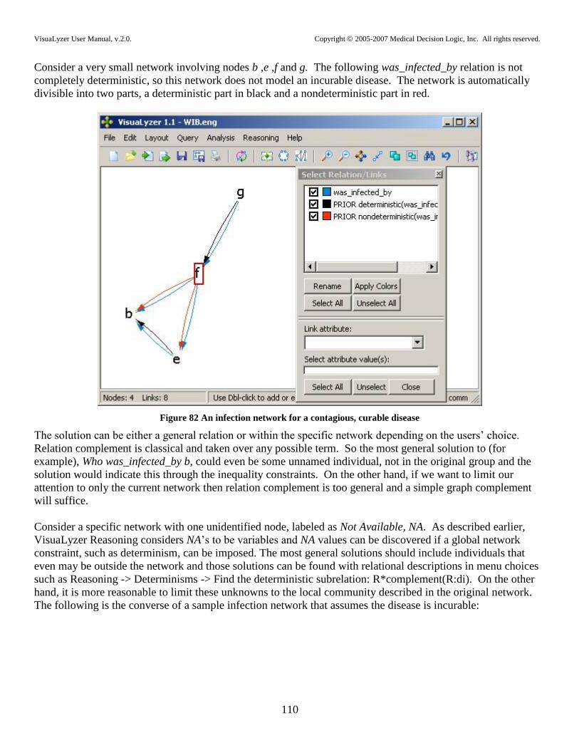
VisuaLyzer User Manual, v.2.0. Copyright 2005-2007 Medical Decision Logic, Inc. All rights reserved.
110
Consider a very small network involving nodes b ,e ,f and g. The following was_infected_by relation is not
completely deterministic, so this network does not model an incurable disease. The network is automatically
divisible into two parts, a deterministic part in black and a nondeterministic part in red.
Figure 82 An infection network for a contagious, curable disease
The solution can be either a general relation or within the specific network depending on the users‟ choice.
Relation complement is classical and taken over any possible term. So the most general solution to (for
example), Who was_infected_by b, could even be some unnamed individual, not in the original group and the
solution would indicate this through the inequality constraints. On the other hand, if we want to limit our
attention to only the current network then relation complement is too general and a simple graph complement
will suffice.
Consider a specific network with one unidentified node, labeled as Not Available, NA. As described earlier,
VisuaLyzer Reasoning considers NA‟s to be variables and NA values can be discovered if a global network
constraint, such as determinism, can be imposed. The most general solutions should include individuals that
even may be outside the network and those solutions can be found with relational descriptions in menu choices
such as Reasoning -> Determinisms -> Find the deterministic subrelation: R*complement(R:di). On the other
hand, it is more reasonable to limit these unknowns to the local community described in the original network.
The following is the converse of a sample infection network that assumes the disease is incurable:
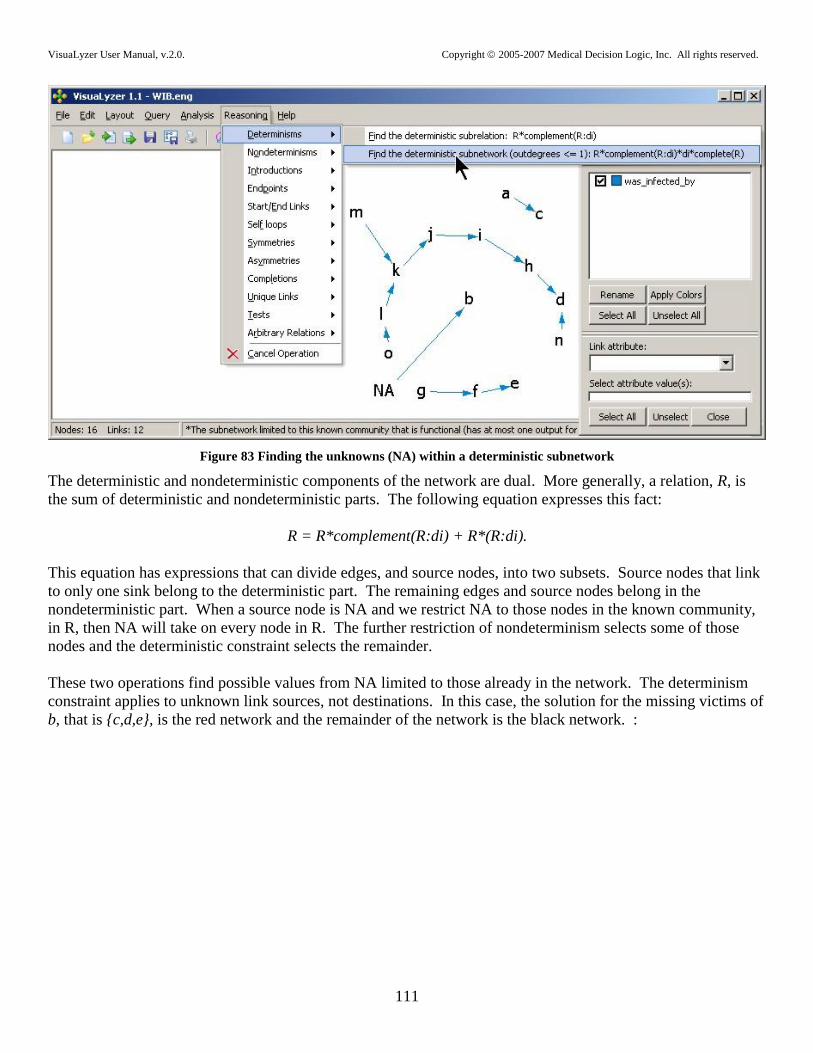
VisuaLyzer User Manual, v.2.0. Copyright 2005-2007 Medical Decision Logic, Inc. All rights reserved.
111
Figure 83 Finding the unknowns (NA) within a deterministic subnetwork
The deterministic and nondeterministic components of the network are dual. More generally, a relation, R, is
the sum of deterministic and nondeterministic parts. The following equation expresses this fact:
R = R*complement(R:di) + R*(R:di).
This equation has expressions that can divide edges, and source nodes, into two subsets. Source nodes that link
to only one sink belong to the deterministic part. The remaining edges and source nodes belong in the
nondeterministic part. When a source node is NA and we restrict NA to those nodes in the known community,
in R, then NA will take on every node in R. The further restriction of nondeterminism selects some of those
nodes and the deterministic constraint selects the remainder.
These two operations find possible values from NA limited to those already in the network. The determinism
constraint applies to unknown link sources, not destinations. In this case, the solution for the missing victims of
b, that is {c,d,e}, is the red network and the remainder of the network is the black network. :
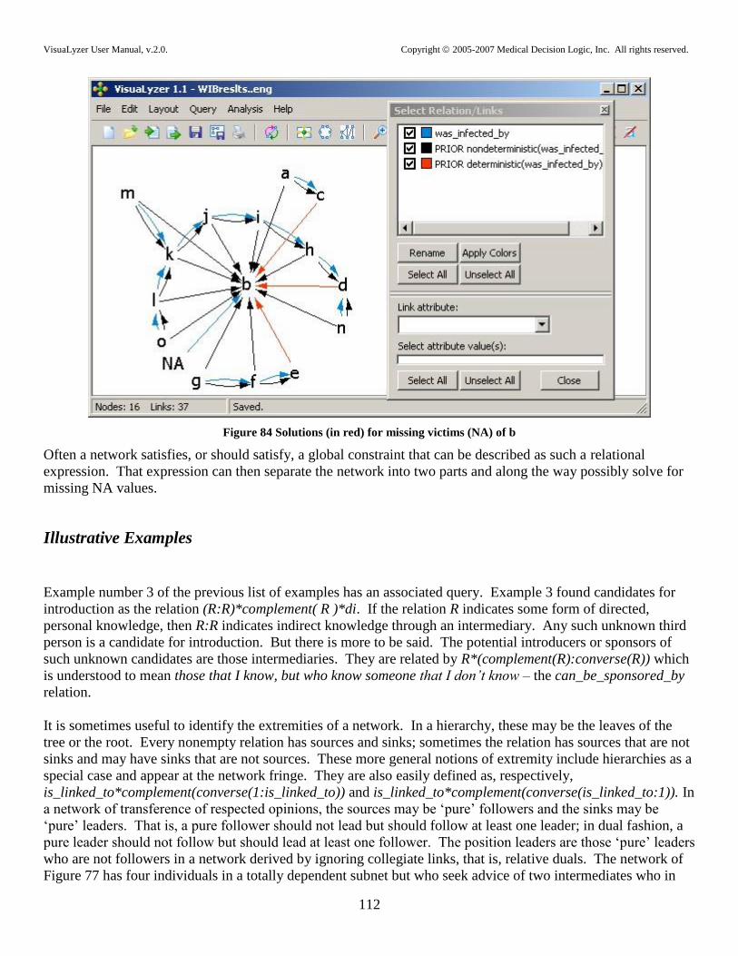
VisuaLyzer User Manual, v.2.0. Copyright 2005-2007 Medical Decision Logic, Inc. All rights reserved.
112
Figure 84 Solutions (in red) for missing victims (NA) of b
Often a network satisfies, or should satisfy, a global constraint that can be described as such a relational
expression. That expression can then separate the network into two parts and along the way possibly solve for
missing NA values.
Illustrative Examples
Example number 3 of the previous list of examples has an associated query. Example 3 found candidates for
introduction as the relation (R:R)*complement( R )*di. If the relation R indicates some form of directed,
personal knowledge, then R:R indicates indirect knowledge through an intermediary. Any such unknown third
person is a candidate for introduction. But there is more to be said. The potential introducers or sponsors of
such unknown candidates are those intermediaries. They are related by R*(complement(R):converse(R)) which
is understood to mean those that I know, but who know someone that I don’t know – the can_be_sponsored_by
relation.
It is sometimes useful to identify the extremities of a network. In a hierarchy, these may be the leaves of the
tree or the root. Every nonempty relation has sources and sinks; sometimes the relation has sources that are not
sinks and may have sinks that are not sources. These more general notions of extremity include hierarchies as a
special case and appear at the network fringe. They are also easily defined as, respectively,
is_linked_to*complement(converse(1:is_linked_to)) and is_linked_to*complement(converse(is_linked_to:1)). In
a network of transference of respected opinions, the sources may be „pure‟ followers and the sinks may be
„pure‟ leaders. That is, a pure follower should not lead but should follow at least one leader; in dual fashion, a
pure leader should not follow but should lead at least one follower. The position leaders are those „pure‟ leaders
who are not followers in a network derived by ignoring collegiate links, that is, relative duals. The network of
Figure 77 has four individuals in a totally dependent subnet but who seek advice of two intermediates who in
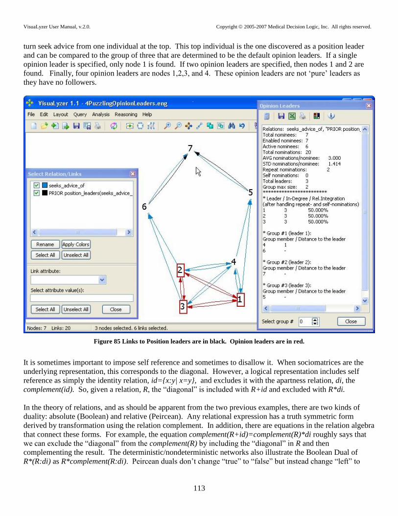
VisuaLyzer User Manual, v.2.0. Copyright 2005-2007 Medical Decision Logic, Inc. All rights reserved.
113
turn seek advice from one individual at the top. This top individual is the one discovered as a position leader
and can be compared to the group of three that are determined to be the default opinion leaders. If a single
opinion leader is specified, only node 1 is found. If two opinion leaders are specified, then nodes 1 and 2 are
found. Finally, four opinion leaders are nodes 1,2,3, and 4. These opinion leaders are not „pure‟ leaders as
they have no followers.
Figure 85 Links to Position leaders are in black. Opinion leaders are in red.
It is sometimes important to impose self reference and sometimes to disallow it. When sociomatrices are the
underlying representation, this corresponds to the diagonal. However, a logical representation includes self
reference as simply the identity relation, id={x:y| x=y}, and excludes it with the apartness relation, di, the
complement(id). So, given a relation, R, the “diagonal” is included with R+id and excluded with R*di.
In the theory of relations, and as should be apparent from the two previous examples, there are two kinds of
duality: absolute (Boolean) and relative (Peircean). Any relational expression has a truth symmetric form
derived by transformation using the relation complement. In addition, there are equations in the relation algebra
that connect these forms. For example, the equation complement(R+id)=complement(R)*di roughly says that
we can exclude the “diagonal” from the complement(R) by including the “diagonal” in R and then
complementing the result. The deterministic/nondeterministic networks also illustrate the Boolean Dual of
R*(R:di) as R*complement(R:di). Peircean duals don‟t change “true” to “false” but instead change “left” to

VisuaLyzer User Manual, v.2.0. Copyright 2005-2007 Medical Decision Logic, Inc. All rights reserved.
114
“right.” The followers/leaders example above and the endpoints and start/end links examples illustrate a
Peircean duality.
The core/periphery procedure described in the previous section sometimes cannot find a core or periphery set of
nodes. This is compared to the procedure for finding the fringe subnet and the remaining middle subnet. The
fringe subnet is simply the sum of the start edges and the end edges. The middle subnet is the rest of the
network that‟s not the fringe. This comparison is illustrated in Figure 86. Those links between the nodes 1, 2,
and 3 comprise the network middle although the network has no core or periphery.
Figure 86 The network middle is in black although there is no core.
A relation is said to be symmetric if it is equal to its converse. Thus a test for symmetry is simply a test of
equality between the two relations. If the relation is infinite, it must have a finite representation. In a
sociomatrix of a finite network, this means that the upper diagonal is a reflection of the lower diagonal. This is
an intuitive description but does not apply to infinite relations. A relation is “Symmetrized up” by summing the
relation with its converse, R+converse(R). A relation is “Symmetrized down” by forming a product of the
relation and its converse, R*converse(R). Similarly, we can find that asymmetric part that is needed to
“Symmetrize up” by subtracting the complement from the converse, converse(R)*complement(R) or find the
extra asymmetric part by subtracting the complement of the converse, R*complement(converse(R)).
If the relation is a network, the graph completion is the set of all possible pairs of nodes of the original network.
Thus, a network involving n nodes has square of n number of edges in the completion. Similarly, the network
complement is the set of new edges. An edge is in the graph complement of R if the edge is not in R.

VisuaLyzer User Manual, v.2.0. Copyright 2005-2007 Medical Decision Logic, Inc. All rights reserved.
115
Finally, it is possible to test a relation, R, for totality by forming 0&R&0. This returns 1, the universal relation,
if the original R was universal and 0 otherwise. Dually, we test for existence of any edge in R by forming
1:R:1. This returns the universal relation, 1, if there exists a pair of nodes in R and 0 otherwise.
Exploring large hierarchies
Sometimes a network, particularly an organizational or ontological structure, is so large that an entire display
has little value. For example, the NCI ontology is a hierarchy of concepts with approximately 33,000 facts that,
when shown in its entirety would likely not illustrate anything useful. This is similar to the organizational
display of a large corporation. The NCI ontology is preloaded into VisuaLyzer at start time from the
userdefined.pl file as an example.
The layered layout of VisuaLyzer is configured by default to incrementally display a large hierarchy from the
top. In order to explore this hierarchy, this top node must have one attribute defined, called hierarchy.
For the beginning node, hierarchy has the value [1] to indicate the top layer. Additionally, the large hierarchy
must have already been defined as a binary relation and preloaded into VisuaLyzer by the file userdefined.pl as
described in the next section.
The figure shows four layers of the NCI ontological hierarchy:
Figure 87 A portion of the NCI ontological hierarchy
For the hierarchy called generalizes, the subsequent steps include menu selections:

VisuaLyzer User Manual, v.2.0. Copyright 2005-2007 Medical Decision Logic, Inc. All rights reserved.
116
Reasoning
Hierarchies
Show hierarchically(generalizes).
Additionally if there are several hierarchies, each is displayed after „Show‟ and within the parentheses after
hierarchically. So one of several hierarchies may be displayed from the list. The preceding figure depicts four
layers of a portion of the NCI ontology defined as a generalizes relation.
Limitations and further information
Note that VisuaLyzer does not display node attribute values that have attributes even though selectors in relative
products can create such deep nesting of attributes. Additionally, relation selectors in VisuaLyzer extract
attributes and can create some nodes with attribute names different from others. If nodes have different
attribute names, then the answer returned from the solution procedure may not be displayed as expected. This
limitation will be removed in the future. Selectors can also produce structures that do not match the
arrangement of attribute - attribute values at all.
The Reasoning part of VisuaLyzer assumes that nodes with identical names, attributes, and attribute values are
identical. This differs from other analysis parts of VisuaLyzer, which consider distinctly drawn nodes to be
different no matter whether they have identical names and attributes or not. A name NA can refer to many
nodes.
Note that a relation complement by itself can be expensive to compute but is not very useful in isolation. Since
it is almost always used in combination with other constraints this is rarely a problem. In particular, if a relation
R has about 20 edges, then complement(R) on its own is barely manageable on a desktop system while the
intersection with a set S (that is, S*complement(R)) of perhaps 1 million edges, can be straightforward.
An attribute has a value or the value is NA. The set expressions in most general form can include inequalities
that can state whether an attribute variable cannot have a value. These inequalities are not represented as
networks but instead, are depicted with more general set expressions.
Avoid equational reasoning on floating point attribute values. This is in part because floating point has always
been approximate arithmetic that may give unintuitive results. Because of the traditional finite binary
representation of floating point numbers presumably true equations may not hold. One example is (10/3)*3 =
10.
Note that an undirected network is considered a symmetric, directed network for these link reasoning purposes.
An undirected link between two nodes is an assertion of both a forward, direct fact and its converse. Thus a
sentence such as ann and bill play cards together would better be described as the pair: ann plays cards with
bill and bill plays cards with ann.
The installation of VisuaLyzer creates an empty file in the default fundamentals folder called userdefined.P.
The user can define other relations such as a large, logical database in this file and it will be loaded at startup.
An example of a logical database of two facts is the file userdefined.P containing the following:
:- op(950,xfy, learned_of_the_innovation_from).
ann learned_of_the_innovation_from bill.
bill learned_of_the_innovation_from carl.

VisuaLyzer User Manual, v.2.0. Copyright 2005-2007 Medical Decision Logic, Inc. All rights reserved.
117
The userdefined.P file is loaded very quickly. On a Windows XP Pentium 4 system, a network of 100,000
edges can load in only a few seconds.
Finally, the menus of VisuaLyzer show the ampersand (&) character as <ampersand>. For example, the relative
sum is not shown as R&S, but is instead shown as R <ampersand> S. Any relational expressions entered
involving the relative sum should use & instead of <ampersand>.
Further Information
For more information, write to [email protected] or [email protected].
Relational reasoning and algebraic logic are described in more detail in
Broome,P. and J. Lipton, Constructive Relational Programming: A Declarative Approach to Program
Correctness and High Level Optimization, Ninth Army Conference on Applied Mathematics and Computing,
1991.
Broome, P. and J. Lipton, Combinatory Logic Programming: Computing in Relation Calculi, International
Logic Programming Symposium, M. Bruynooghe, Ed., MIT Press, 1994.
Jonsson, B., The theory of binary relations, Colloq. Math. Soc., János Bolyai 54, Algebraic Logic, Budapest,
Hungary (1988), 245-292.
Tarski, A. and S. Givant, A formalization of set theory without variables, AMS Colloquium Publications Vol
41, AMS Providence R.I., 1987.
Wasserman, S. and K. Faust, Social Network Analysis: Methods and Applications, Cambridge University Press,
Cambridge, UK, 1994.
Broome, P. and J. Lipton, Combinatory Logic Programming: Computing in Relation Calculi, International
Logic Programming Symposium, M. Bruynooghe, Ed., MIT Press, 1994.
Broome, P., Relations and Constraints for Constructive Programming, SSGRR-2000, International Conference
on Advances in Infrastructure for Electronic Business, Science and Education on the Internet, Scuola Superiore
G. Reiss Romoli, L‟Aquila, Italy, Aug 2, 2000.

VisuaLyzer User Manual, v.2.0. Copyright 2005-2007 Medical Decision Logic, Inc. All rights reserved.
118
Appendix: Mouse and Keyboard Commands
Mouse Right Button Click popup command menu
Mouse Right Button Click+Drag+Release add link (Click on from_node - Release on to_node
or on empty space on canvas; if to_node not exists
it will be created and connected to from_node)
Click If click on empty space on canvas - unselect all,
else select node or link (link is selected if nodes on both ends are selected)
Click on node/link label does the same!
Click+Drug If click on node - move selected node(s),
else if click on link - move selected link(s) together with connected nodes,
else if click on empty space - select number of nodes/links (group selecting)
Drop node(s) on group node
Add selected node(s) to the group.
Double-Click If click on empty space on canvas - add new node,
else edit selected node or link properties.
Shift-Click Select another node or link while preserving other nodes/links selection
Ctrl-Click Disable/Enable selected node.
Alt-Click Freeze/Unfreeze selected node position
F1 Context help (currently under development)
F2 Edit node/link properties (whatever is selected)
F3 Toggle node attributes windows On/Off (for selected nodes only)
F4 Edit display properties (appearance and behavior settings; depends on node/link selection)
F5 Add new node
F6 Straighten out links
F7 Add new link (endpoint nodes have to be selected)
F8 Create group
F9 Spring-Embedding Layout start/stop (get organized!)
F10 Best fit
F12 Toggle mouse mode (magnifier/regular)
Del Disable/Enable selected nodes (disabled nodes are ignored during calculations)
Ctrl<+> Zoom In
Ctrl<-> Zoom Out
Ctrl+A Select all nodes (if graph component has focus)
Ctrl+C Copy selected nodes/edges to Clipboard
Ctrl+F Find node by label (pattern search)
Ctrl+L Open Legend screen
Ctrl+N New file
Ctrl+O Open file (VisuaLyzer binary .eng file)

VisuaLyzer User Manual, v.2.0. Copyright 2005-2007 Medical Decision Logic, Inc. All rights reserved.
119
Ctrl+R Run Relational Expression Builder
Ctrl+Q Run search query
Ctrl+S Save file (VisuaLyzer binary .eng file)
Ctrl+T Open Select Relation/Type screen
Ctrl+V Paste nodes/edges from Clipboard
Ctrl+W Load and apply a View
Ctrl+X Cut selected nodes/edges
Ctrl+Z Undo last operation