Grand Valley State UniversityScholarWorks@GVSU

Masters Theses Graduate Research and Creative Practice

7-28-2017

Visualization of the Cardiac Excitation and PVCArrhythmia on a 3D Heart ModelPranav Sreedharan VeliyaraGrand Valley State University

Follow this and additional works at: http://scholarworks.gvsu.edu/theses

Part of the Engineering Commons

This Thesis is brought to you for free and open access by the Graduate Research and Creative Practice at ScholarWorks@GVSU. It has been acceptedfor inclusion in Masters Theses by an authorized administrator of ScholarWorks@GVSU. For more information, please contactscholarworks@gvsu.edu.

Recommended CitationSreedharan Veliyara, Pranav, "Visualization of the Cardiac Excitation and PVC Arrhythmia on a 3D Heart Model" (2017). MastersTheses. 851.http://scholarworks.gvsu.edu/theses/851

Visualization of the cardiac excitation and PVC arrhythmia on a 3D heart model

Pranav Sreedharan Veliyara

A Thesis Submitted to the Graduate Faculty of

GRAND VALLEY STATE UNIVERSITY

In

Partial Fulfillment of the Requirements

For the Degree of

Master of Science in Engineering

School of Engineering

August 2017

3

Acknowledgements

I would like to thank first my thesis advisor Dr. Samhita Rhodes for her continuous

guidance and support throughout my studies at Grand Valley State University (GVSU). She

has been a wonderful thesis advisor.

I would also like to thank my thesis committee members Dr. Robert Bossemeyer and Dr.

Nicholas Baine for their valuable inputs for this thesis. Their participation helped me to

conduct my research successfully.

I would like to thank Mr. Eric VanMiddendorp, former student at GVSU for providing

necessary reference documents and research materials to start my thesis. I would also like to

thank Mr. Deepak Dileepkumar, former student at GVSU for helping me with the

implementation of the Graphical User Interface design in MATLAB.

I would like to thank all the staff and faculty of GVSU who directly or indirectly helped

me to conduct my research.

Finally, I would like to thank my parents, family and friends for their continuous support

and encouragement.

Pranav Sreedharan Veliyara

4

Abstract

Visualization of the cardiac potential movement is important in understanding the

physiology of the human heart. A 3D visualization tool will help the cardiology students and

others interested in human physiology to understand the functioning of the heart. In this

thesis, such a tool is proposed which helps in the visualization of the cardiac potential

movement and Premature Ventricular Contraction (PVC) event on a 3D heart model. The

cardiac excitation obtained from a limb lead and a precordial lead of a 12 lead

electrocardiograph (ECG) is mapped on a 3D heart model with fixed conduction pathways.

The 3D heart model is obtained by modifying an existing anatomically accurate heart model.

Fixed conduction pathways are defined on this derived 3D heart model. Each component of

the ECG corresponds to the potential movement along each segment of these conduction

pathways. The timing information from the limb lead signal is used to map the position of the

cardiac potential on these conduction pathways. Amplitude and the timing information

obtained from the precordial lead is mapped on a vector which points towards the

corresponding precordial electrode on a separate window. This helps in understanding the

instantaneous position of the cardiac potential on the transverse plane. Mapping of the cardiac

excitation on the conduction pathways will stop and the color map of the heart will change

during the occurrence of a PVC event. MIT-BIH arrhythmia database signals with at least

one PVC wave were considered as input signal. It is observed that the system was able to

detect PVC approximately 95% of the time (for the selected sample signals) and was able to

map each ECG component accurately on the conduction pathways with minimum mapping

delay.

5

Table of Contents

1. Introduction 11

2. Literature Review 13

2.1. Background 13

2.1.1. Physiology of cardiac excitation 13

2.1.1.1. Conduction pathway 15

2.1.2. Electrocardiogram 17

2.1.2.1. Lead placements 19

2.1.2.2. Limb leads 20

2.1.2.3. Augmented limb leads 22

2.1.2.4. Precordial leads 22

2.2. Visualization of the human heart 23

2.2.1. 2-Dimensional heart models 24

2.2.2. 3-Dimensional heart models 25

2.3. PVC arrhythmia 27

3. Specific Aims 28

4. Methodology 29

4.1. QRS detection module 30

4.2. PVC detection module 31

4.2.1. Sum of trough (ST) 32

4.2.2. Sum of Rpeak with minimum (SumMin) 33

4.3. 3D heart envelope 34

6

4.4. Cardiac potential mapping 36

4.4.1. Conduction pathways 36

4.4.2. Timing information and mapping 39

4.5. Chest lead potential mapping 42

5. Results 44

5.1. 3D envelope 44

5.2. Input signal 45

5.3. Mapping 49

5.3.1. Lead II mapping 52

5.3.2. Precordial lead mapping 55

5.4. PVC detection and mapping 57

6. Analysis and Discussion 62

7. Conclusion 72

8. Appendix I – Source code 74

8.1. GUI 74

8.2. Timing information 79

8.3. Heart envelope 82

8.4. PVC detection 84

8.5. Precordial lead vector 85

8.6. Running signal plots 88

8.7. Main function with conduction pathways and the cardiac potential mapping 90

9. Appendix II – QRS detection model 98

9.1. Denoising 98

7

9.2. QRS-complex detection 99

9.3. P-wave detection 101

9.4. T-wave detection 102

10. Appendix III – References for the current research in cardiology 104

11. References 105

8

List of Tables

Table 1 Twelve lead ECG electrode placement on the human body 19

Table 2 Time variables corresponding to each ECG segment 40

Table 3 ECG signals with PVC from the MIT-BIH database 45

Table 4 Timing information form lead II 50

Table 5 PVC peak detection results 61

Table 6 Atrial and Ventricular mapping delays 63

Table 7 True positive analysis on signal 100 69

Table 8 True positive analysis on signal 114 69

Table 9 True positive analysis on signal 116 70

Table 10 True positive analysis on signal 119 70

Table 11 PVC detection algorithm efficiency study 71

Table 12 Decomposed signal coefficients and corresponding frequencies 99

9

List of Figures

Figure 1 Heart anatomy [2] 13

Figure 2 Wigger's diagram [3] 15

Figure 3 (A) 2D representation of conduction pathway with labels [4], (B) 3D model of the

human heart and the conduction pathway [5] 16

Figure 4 Twelve lead ECG [6] [21] 18

Figure 5 Lead placement - 12 lead ECG [7] 19

Figure 6 Lead vector motion with respect to ECG segments (P and Q) [8] 21

Figure 7 Lead vector motion with respect to ECG segments (QRS and T) [8] 22

Figure 8 (A) Planes with respect to the human body [9] and (B) the lead placement angles 23

Figure 9 Malchenko’s. Contours (left), 3D heart surface (right) [12] 25

Figure 10 Output window of ECGSIM for a 12 lead input ECG signal 26

Figure 11 Proposed 3D heart visualization system 29

Figure 12 ECG delineation in MIT-BIH ECG signal - 105 30

Figure 13 PVC detection algorithm flowchart 31

Figure 14 PVC detection thresholds 34

Figure 15 Malchenko’s 3D heart model [20] 35

Figure 16 Co-ordinates of the conduction pathways 37

Figure 17 Different regions of the derived heart model 38

Figure 18 Cross sectional image of the chest and precordial leads [24] 43

Figure 19 (A) 3D heart, and (B) its cross section along frontal plane 44

Figure 20 (A) Conduction pathway, (B) Conduction pathway mapped on to the masked 3D

heart model (right) 45

Figure 21 Signal 101 with no PVC (Upper: Lead II, Lower: V1) 47

Figure 22 Output waveforms of QRS detection module for signal 101 (A: Lead II, B: V1) 48

Figure 23 Signal 114 (Upper: Lead V5, Lower: II) 49

10

Figure 24 Output window 51

Figure 25 Mapping of the P wave on the conduction pathways 53

Figure 26 Mapping of the PQ segment on the conduction pathways 53

Figure 27 Mapping of the QRS complex on the conduction pathway 54

Figure 28 Mapping of the ST segment on the conduction pathway 55

Figure 29 Chest lead potential mapping during P wave 56

Figure 30 Chest lead potential mapping during an Rpeak 56

Figure 31 Chest lead potential mapping of a PQ segment 57

Figure 32 Chest lead potential mapping during a negative amplitude 57

Figure 33 Detected PVC peaks on the signal 100 (Upper: Lead II, Lower: V5) 58

Figure 34 PVC peaks on signal '114' near 8.31min 59

Figure 35 PVC peaks on signal '119' near 1.55min 60

Figure 36 PVC mapping 61

Figure 37 Signal 100 - Lead II (First 5 minutes) 65

Figure 38 Signal 114 - Lead II (First 5 minutes) 66

Figure 39 Signal 116 - Lead II (First 5 minutes) 67

Figure 40 Signal 119 - Lead II (First 5 minutes) 68

Figure 41 True positive rate analysis chart 69

11

1. Introduction

One of the most complex organs in the human body is the heart. The heart, along with

other components in the circulatory system - arteries, veins, lymph vessels and lymph nodes

coordinate blood circulation. Cardiac potentials generated by the myocardial cells result in

the cardiac contraction and the circulation of blood through the rest of the body. Each normal

heart beat is the result of an action potential, originating in the sinus node, which spreads

through the atrial and ventricular muscle cells resulting in a coordinated pumping action. This

spread of excitation can be recorded on the surface of the body by an electrocardiogram

(ECG). Abnormalities in this cardiac potential generation or disruptions in cardiac conduction

can cause arrhythmias and complications in the circulation of oxygen and nutrients to the

brain and body.

Difficulties in determining cardiac pathology and the complexity of the heart structure

itself makes ECG signal processing a very valuable focus of research. Some of the cardiac

signal processing studies involve arrhythmia analysis, wireless pacemaker design, and cardiac

function irregularity studies, to name a few. Various physical and software tools are available

to make the task of visualizing heart function easier for cardiologists in training. These tools

can also be used by cardiac surgeons to explain procedures to patients and caregivers

unfamiliar with cardiac anatomy and function.

A majority of the software tools are not readily available to the lay population and can be

expensive. One of the few freeware tools available online is ‘ECGSIM’, a simulation tool

developed by the scientists at Radboud University Medical Center, Netherlands. ECGSIM is

a visualization tool which displays cardiac potential spread as a field movement on the

surface of a 3D heart model. It has a definite set of input signals and a unique 3D heart

model. ECGSIM can also demonstrate electrical characteristics, and simultaneously display

12

the spread of the potential over the thorax. However, this model does not provide any

information about possible conduction pathways. Input signals are not continuous and just

limited to a single heartbeat. In addition, arrhythmias are not modeled in ECGSIM.

The primary objective of this project is to develop a 3D ECG visualization educational

tool for medical students undergoing cardiology training, and patients wanting to learn about

cardiac procedures. This thesis represents the second phase of that bigger project [1]. In this

thesis, a novel heart visualization tool is proposed which is an interactive MATLAB based

tool that can visualize a continuous ECG signal with cardiac conduction pathways. A

premature ventricular contraction (PVC) arrhythmia detection module is also part of the

proposed system. Other modules are the QRS detection and 3D mapping modules. ECG

signals from the MIT-BIH arrhythmia database are used as input signals. This system also

helps the user to visualize the relation of the potential movement with the corresponding

precordial lead vector. The PVC detection algorithm developed for this thesis uses multiple

thresholds in a unique combination to determine whether a given Rpeak is a PVC peak or not.

There are two levels in this thresholding hierarchy. Screening using the first threshold which

is an average Rpeak to Rpeak interval is performed in the first level. Data that qualifies this

threshold is further screened in the second level using the other two thresholds. If the

screened data qualifies either of these thresholds in the second level, it is identified as a PVC

peak. The first threshold searches for large Rpeak to Rpeak intervals, the second threshold finds

abnormally large Rpeaks and the third threshold finds the negative peaks.

13

2. Literature Review

2.1. Background

2.1.1. Physiology of cardiac excitation

The human heart is four chambered with two thin walled upper chambers called the atria

and two thicker walled lower chambers called the ventricles. The right atrium and the right

ventricle is involved in the pulmonary circulation by sending deoxygenated blood arriving

from the different organs to the lungs for oxygenation. The left atrium and ventricle is

responsible for systemic circulation by receiving oxygenated blood from the lungs and

distributing to the rest of the body. Thus, the two circulatory components are completely

isolated from one another. This prevents the oxygenated and the deoxygenated blood from

mixing. Figure 1 shows the anatomy of the mammalian heart.

Figure 1 Heart anatomy [2]

14

The heart wall is made up of cardiac muscles, composed of strong muscle fibers which is

unique compared to the other muscle fibers in the body. Certain groups of smaller muscle

cells do not contribute to the pumping action due to their weak contractile feature. The SA

node is one such group of cells. It acts as the pacemaker of the heart. These cells rhythmically

produce action potentials which spread via gap junctions to the fibers of both atria. Gap

junctions are the intercellular connections which transports nutrients and electrical signals.

This potential flow results in the atrial contraction and subsequent ventricular contraction

rhythmically, which causes a heartbeat. The action potential which is generated from the SA

node reaches the atrioventricular (AV) node at the junction between atria and ventricles, and

then moves rapidly through the bundle of His and Purkinje fibers to excite both ventricles,

which then contract. This synchronous electrical activity is necessary for the mechanical

contraction of the heart. These recorded signals are popularly known as an electrocardiograph

(ECG), which is the electrical activity of the heart with respect to the ground electrode.

Figure 2 is a Wigger’s diagram which shows the relation of the cardiac activities with an

ECG segment.

15

Figure 2 Wigger's diagram [3]

An ideal ECG wave with peaks labelled, can be observed in the Wigger’s diagram. ECG

is composed of three phases: atrial depolarization, ventricular depolarization, and ventricular

repolarization in preparation for the next beat. P-wave is produced by the atrial

depolarization. QRS complex is produced by the ventricular depolarization and the atrial

repolarization. Signal strength of the atrial repolarization is negligible compared to the

ventricular depolarization. T-wave is produced by the ventricular repolarization.

2.1.1.1. Conduction pathway

The electric potentials generated from the SA node travel along well-defined paths to

complete one cardiac cycle. As mentioned earlier, the first segment of this path connects the

16

SA node and the AV node. Then the potential is delayed for approximately a tenth of a

second in the AV node and then moves to the bundle of His and Purkinje fiber.

Figure 3 (A) 2D representation of conduction pathway with labels [4], (B) 3D model of the

human heart and the conduction pathway [5]

Components of the conduction pathways shown in the Figure 3 are as follows:

SA node – Sino Atrial node is the natural pacemaker of the human heart. This node is

located in the myocardium just internal to the epicardium situated on the inner wall of

the right atrium, where superior vena cava enters the chamber. An action potential

generated in the SA node, spreads from cell to cell starting in the right atrium.

Simultaneously, the Bachmann’s bundle conducts the potential to the left atrium.

Paths that the cardiac potential is spread throughout the right atrium are known as the

internodal pathways, after which the potential reaches the AV node.

Internodal pathways – Paths which connect the SA node to the AV node are known as

internodal pathways. There are three internodal pathways: posterior or Thorel’s tract,

middle or Wenckebach’s tract, and anterior internodal tract. The anterior internodal

path projects a branch to the left atrium which is known as Bachmann’s bundle.

17

AV node – The Atrio Ventricular node is located at the lower side of the interatrial

septum near the coronary sinus opening. Cardiac potential delays at the AV node for a

fraction of a second. Atria pumps blood into the ventricle during this delay. Only after

this delay do the ventricles contract. Hence, AV node and this delay is critical in

maintaining the pace of the cardiac cycle. Prolonged delay or atrial depolarization’s

inability to reach the AV node are the most common abnormalities which can cause

several arrhythmias.

Bundle of His – The bundle of His is located at the inferior side of the interatrial

septum. It helps to transmit the cardiac potential impulse from the AV node to the

ventricles. As shown in Figure 3, the conduction pathway divides into two branches

from the bundle of His. One path towards the left ventricle and the other path towards

the right ventricle through interventricular septum. The left branch further divides into

left anterior and left posterior fascicles.

Purkinje fiber – Purkinje fibers are the last segment of the conduction pathways.

Purkinje fibers extend from the bundle of His and then spread along both ventricle

walls. QRS segment in the ECG signal is a result of the spread of cardiac potentials

from the bundle of His to the Purkinje fibers and through the ventricular cardiac

muscle. Impulse firing rate of the Purkinje fibers is 15 to 40 beats per minute.

Abnormal cardiac potential generated from the Purkinje fibers are known as

Premature Ventricular Contractions (PVC). PVCs are one of the most common

arrhythmias.

2.1.2. Electrocardiogram

The cardiac excitation is recorded in various different ways: three lead ECG system,

twelve lead ECG system, vector cardiogram (VCG), and phonocardiogram are some of these

techniques. Twelve lead ECG system is the most popular one. This ECG system records

18

information of the electrical activity from all three orthogonal planes using its unique lead

placement. ECG data for normal sinus rhythm from a standard 12 lead recording system is

shown in the Figure 4. Simultaneously obtained data from the two leads of the standard 12

lead system (MIT-BIH arrhythmia database) is used as input signal in this thesis. Lead II

(only available limb lead data in the MIT-BIH arrhythmia database) is used as the channel 1

input and any available precordial lead is used as the channel 2 input.

Figure 4 Twelve lead ECG [6] [21]

19

2.1.2.1. Lead placements

The 12 lead ECG system is composed of two groups of leads, each consisting of 6 leads.

6 limb leads and 6 precordial leads (or generally known as chest leads). The limb leads are

bipolar and precordial leads are unipolar. Three of the 6 limb leads are augmented leads.

Figure 5 shows the lead vectors of a standard 12 lead ECG system. Electrode placement on

the subject’s body is as listed in the Table 1. Combination of the potentials at these electrodes

are used to derive lead vectors.

Figure 5 Lead placement - 12 lead ECG [7]

Table 1 Twelve lead ECG electrode placement on the human body

Electrode Electrode placement

Right Arm (RA) Near inner side of the right hand wrist

Left Arm (LA) Near inner side of the left hand wrist

Right Leg (RL) On the right leg lateral calf muscle.

20

Left Leg (LL) On the left leg lateral calf muscle.

V1 Between 4th and 5th ribs, near the right side of the sternum

V2 Between 4th and 5th ribs, near the left side of the sternum

V3 Between leads V2 and V4.

V4 Between 5th and 6th ribs, near mid-clavicular line

V5 Horizontal with V4, on the left anterior axillary line.

V6 Horizontal with V4 and V5,on the mid-axillary line.

2.1.2.2. Limb leads

The limb lead potentials are measured using the electrode potential differences as follows.

Lead I: VI = LA- RA (2.1.2.2.1)

Lead II: VII = LL-RA (2.1.2.2.2)

Lead III: VIII = LL-LA (2.1.2.2.3)

Since two electrodes are required to derive one lead potential, these leads are known as

bipolar leads. According to Einthoven's lead system, it is assumed that the heart is located at

the center of a homogeneous sphere representing the torso [8]. RA, LA, and LL leads are

positioned at the vertices of an equilateral triangle inside this sphere, with the heart located at

its center. Three vectors are formed connecting two electrodes at a time. They are lead I, II

and III vectors. Vector sum of the two of these leads results in the third lead’s potential. This

is stated by Einthoven’s law and the equilateral triangle is known as Einthoven’s triangle.

Vector sum of the three leads are mapped on the Einthoven’s triangle.

Figure 6 and Figure 7 shows the relation between the potential movement and the cardiac

vector. At a given time, position of the cardiac potential on the heart and the corresponding

lead vector potential on Einthoven’s triangle can be observed from these figures. The red

21

colored region on the heart shows the potential spread and the blue region is the remaining

portion of the heart. The yellow vector inside the Einthoven’s triangle is the resultant cardiac

vector. Path traced by this vector’s head is shown in green color. Vector components along

each side of the triangle gives the individual limb lead potential. Corresponding potential is

mapped as ECG. The cardiac potential’s movement from atria to ventricle and the generation

of P, Q and Rpeaks can be observed from Figure 6. Remaining ECG components and

corresponding cardiac potential can be observed from Figure 7.

Figure 6 Lead vector motion with respect to ECG segments (P and Q) [8]

22

Figure 7 Lead vector motion with respect to ECG segments (QRS and T) [8]

2.1.2.3. Augmented limb leads

Augmented limb leads are pointed in different directions compared to the limb leads.

These lead vectors are pointed towards the vertices of the Einthoven’s triangle from the

center region. Augmented lead vectors are derived using Goldberg’s central limit theorem

which is the sum of the three limb electrodes in a unique combination. Augmented limb leads

are not used as input signals in this thesis.

2.1.2.4. Precordial leads

This is a set of 6 electrodes placed on the left side of the chest, near the heart along the

transverse plane. These leads are unipolar vector and originates at a common lead or

commonly known as Wilson’s central terminal. The Wilson’s central terminal is obtained by

averaging the potential at the limbs with reference to the electrode on the right leg using three

23

identical resistors (≥5 kΩ) connected to a single point. This terminal is assumed as negatively

charged and the precordial leads are positively charged. Wilson’s central limit theorem,

VW = 1

3(RA + LA + LL) (2.1.2.4.1)

Where,

VW = Wilson’s central terminal

Each lead is placed 30O apart from the previous lead. See Figure 8 to understand the

direction of the leads (V1 to V6) in the transverse plane.

Figure 8 (A) Planes with respect to the human body [9] and (B) the lead placement angles

2.2. Visualization of the human heart

Research in cardiology ranges from electronic health record systems to artificial invasive

pacemakers (refer Appendix III for related reference documents). These studies include

visualization as well. The primary objective of this thesis is to visualize heart activity on a 3D

24

space. The following sub sections discuss current research on 2D and 3D visualizations of the

human heart. The visualization of normal sinus rhythm and PVC arrhythmia are proposed and

implemented as part of this thesis.

2.2.1. 2-Dimensional heart models

Sovilj’s heart model [10] is a 2D heart model where all the conduction pathway

components are labelled. This is a bi-domain finite element heart model which uses color

variation to represent the movement of the electric potential through the walls. This model

was developed using COMSOL Microphysics, a finite element analysis software. A 2D

model with a very high anatomical accuracy was developed in this research. Volume

conductor effects of blood, tissues, and torso were accurately matched to develop the 2D

heart model using COMSOL features. Constraints such as conductivity of the heart tissues

and blood tissues can be adjusted using COMSOL. Modified FitzHugh-Nagumo [10] method

was used in this model to simulate the various electrical activities.

Second model is Balakrishnan’s model [11], a simplified 2D model which shows the

potential spread on a 2D image of the conduction pathway. This model is essentially a cell

network. Individual cells changes state based on the position of the electric potential. Each

state is represented by a different color. Each cell is connected to the neighboring 8 cells. A

gap junction is present between the cells. Conductance of this junction is varied based on the

properties of the tissue which the cell represents. When potential conducts from one cell to

another, the state of the previously excited cells and current cell are changed to different

colors. Electrical activity mapping and 2D network is developed using reduced FitzHugh -

Nagumo model [11] and Aleiv – Panfilov model [11].

25

2.2.2. 3-Dimensional heart models

A 3D heart model was developed in Malchenko’s research [12] [20]. In this model, an

envelope of the human heart was reconstructed from the MRI images using MATLAB.

Coordinates from 10 time moments were recorded for this reconstruction. Each time moment

consists of 16 images of the heart. A contour is sketched connecting the coordinates obtained

from each image. Collection of these contours corresponding to each time moment were used

to draw splines across the heart surface. A 3D heart envelope is obtained from these contours

and vertical splines. Figure 9 shows the contours and the resultant 3D structure of the heart.

Internal properties of the heart including the position and dimension of the chambers, walls,

septum, and valves are not considered in this design. This heart model is used for several

other research [13] [14] to study the heart’s functionality during various arrhythmias. Due to

its unique structure that is anatomically correct and since it is available as open source,

Malchenko’s 3D model is used to build the simulation tool discussed in this thesis.

Figure 9 Malchenko’s. Contours (left), 3D heart surface (right) [12]

Second 3D model is ECGSIM [15], a simulation software which helps the user to study the

relation between ECG and cardiac potential flow on the surface of the heart. This software

can display input signal as 12 lead ECG, VCG, body surface map (BSM), minimap montage

(using 9 electrodes), and single lead ECG. The corresponding potential spread is displayed on

26

the surface of a unique 3D heart surface as shown in Figure 10 which is the output window of

ECGSIM.

Figure 10 Output window of ECGSIM for a 12 lead input ECG signal

In Figure 10, the 3D heart model can be observed in the top left corner. The torso can be

seen on the top right corner. The position of the heart inside the torso can also be observed.

The bottom left graph is the transmembrane potential of a selected node. The bottom right

window is the input signal display window. The 3D model allows the user to select single or

multiple nodes on the heart surface to set constraints like amplitude parameters or slope

parameters of transmembrane potential. Corresponding changes can be visualized on the

ECG display window. Potential spread on the 3D heart will not change based on this

selection. Color mapping represents the time (in ms) at which activation wave front reaches

each region. Even though ECGSIM is a complete simulation package, it has some major

limitations. ECGSIM cannot accept external input signals. User does not have freedom to

input a recorded ECG signal or a real time ECG signal to the system to visualize its

properties. In addition, ECGSIM does not give any information about any kind of arrhythmia.

27

Third 3D model is ‘the living heart project’ [16], a 3D heart model developed by Dassault

Systems. This model is built on Simulia, a simulation suite of Dassault Systems. It can

display activities of a human heart in a realistic way. Virtual reality experience is the unique

feature of this model. It helps in better visualization of the heart diseases as well. Physician

can visualize the abnormality in the functioning of the heart using the virtual reality feature

and propose suitable surgery or medication. PVC event visualization implemented in this

thesis is inspired from this system.

2.3. PVC arrhythmia

Premature Ventricular Contractions have some unique properties compared to the normal

sinus beat. Longer QRS duration and larger peaks of the PVC make it easy to detect

manually. Fluttering, pounding, skipped beats etc. are some of the most common symptoms

of PVC. During a PVC, ventricles contracts before atrial depolarization completes.

Even though PVCs do not occur often in a given time interval, certain types of PVCs

occur at regular intervals. As the name suggests, the bigeminy PVC occur in every other beat,

the trigemini in every third beat, and the quadrageminy in every fourth beat. Paired PVC has

a unique feature of two abnormal peaks every occurrence. There are more varieties of PVCs.

A common feature is the uniqueness in the time interval and amplitude compared to a normal

beat. Some of the most common algorithms used to detect PVCs are template matching

algorithm [17], Bayesian detection [18], and wavelet-transform based algorithms [19].

Even though PVC on a healthy patient is no reason for concern, PVC coupled with other

health conditions can be associated with various diseases. For example, recent studies shows

that the frequent PVCs may result in causing heart failure in patients with dysfunctional left

ventricle [23]. PVC can be dangerous to the patients suffering from coronary artery disease or

valve disease. Thus it is important to detect and track the frequency and amplitude of PVCs.

28

3. Specific Aims

In this thesis, following steps were conducted to develop a 3D visualization model of the

cardiac activity.

Develop or obtain an anatomically accurate MATLAB readable digital 3D heart

model.

Define conduction pathways using this 3D heart model.

Obtain cardiac excitation signal and remove noise.

Obtain the timing information corresponding to each cardiac activity using this signal.

Map the cardiac excitation signal on the respective 3D space of the heart model based

on the timing information.

Implement PVC arrhythmia detection module using a suitable peak detection

algorithm.

Test the efficiency of the system using accuracy test and running time test.

Evaluate the specificity and sensitivity of the PVC detection algorithm.

The expected end product is a GUI based software which can be used as an

educational tool.

29

4. Methodology

This section describes the algorithms used to implement the proposed ECG visualization

tool. All five modules are implemented using MATLAB 2015. MIT BIH arrhythmia database

signals are used as input signals. This database is a collection of 30 minutes long 48

recordings performed on 47 subjects. It consists of 2 channels. In majority of the recordings,

first channel consists of a limb lead signal (lead II in most of the signals) and the second

channel consists of a precordial signal. The lead II and a precordial lead signal sampled at

360Hz frequency are the available information for most of the recordings in this database. So,

these orthogonal leads are used in this thesis for visualizing the heart activity. Figure 11 is the

functional block diagram of the proposed system. Main features of the system are as follows:

An interactive MATLAB based GUI.

Anatomically accurate 3D heart envelope.

3D visualization of the conduction pathway.

Visualization of the movement of cardiac visualization using ECG segment timing

information.

Robust PVC arrhythmia detection algorithm.

Morbidity warning system.

Figure 11 Proposed 3D heart visualization system

30

4.1. QRS detection module

This module was implemented in the first phase of this project in a Grand Valley State

University master’s project titled ‘Electrocardiogram Delineation Method Using Wavelet

Transform and Novel Display Method [1]’. This is a wavelet transform based ECG feature

extraction module implemented in MATLAB using delineation algorithm. ‘Symlet’ wavelet

transform is used to decompose the raw signal into 8 levels, each representing different

frequency ranges. Frequency components corresponding to low frequency noise are

subtracted from the original signal and the high frequency noise is eliminated using a soft

thresholding method. A set of adaptive windowing and adaptive thresholding is used to

extract fiducial points from this denoised signal. These fiducial points are mapped on the

original signal and displayed as output waveform. The algorithm is detailed in Appendix II.

Figure 12 is a sample output obtained from this module after processing a raw ECG signal.

Fiducial points Rpeak, QRSon, QRSoff, Ppeak, Pon, Poff, Tpeak, and Tend are exported to the

potential mapping module to obtain the timing information.

Figure 12 ECG delineation in MIT-BIH ECG signal - 105

31

4.2. PVC detection module

Wider Rpeak to Rpeak intervals (RRI) compared to the mean RRI, early occurrence of the

QRS complex and larger peak amplitudes compared to the normal ECG waves are the

common characteristics of PVCs. As mentioned earlier, PVCs can occur at regular intervals,

but not always. The frequency of PVCs possibly suggest a health condition of the subject.

Following flowchart (Figure 13) demonstrates the PVC detection algorithm developed for

this thesis.

Figure 13 PVC detection algorithm flowchart

32

This algorithm is adapted from the Chang’s model [19] with a modification in the

combination of the threshold usage. The PVC peaks are detected using three different

thresholds in both algorithms. However, unlike in Chang’s model, an Rpeak is identified as a

PVC peak even if one of the 2nd or the 3rd threshold fails. First threshold is an average RRI

computed from the lead II input signal.

First threshold,

PVCThr =tRpeak[end]−tRpeak[1]

l−1 (4.2.1)

where,

l = number of Rpeaks

tRpeak [i] = location of the Rpeak at the location [i] in ms

Every RRI of the input signal are compared with the average RRI. If the RRI of the

current wave segment (time interval between current and next Rpeak) is greater than this

threshold, current wave is identified as unique. Further conditions will determine if it is a

PVC wave or not. Second and third thresholds are more focused on detecting abnormally

large positive and negative amplitudes.

4.2.1. Sum of trough (ST)

Second threshold used in the PVC detection is known as sum of trough. In every iteration,

an Rpeak is considered for PVC detection. In a particular iteration, amplitude of the 50

locations after the current Rpeak location are added together. If this value is less than zero, that

particular peak is detected as a PVC peak.

SumT = ∑ amp[tRpeak[i] + n]50

n=1 (4.2.1.2)

where,

33

amp(x) = Amplitude at location x in mV

4.2.2. Sum of Rpeak with minimum (SumMin)

Third threshold used in this thesis to detect PVC wave is sum of Rpeak with minimum. This

is a summation equation as defined in equation 4.2.2.1. In any particular iteration, the

minimum amplitude between the two consecutive Rpeaks is added to the current Rpeak. If this

value is less than zero, the current Rpeak is identified as a PVC.

SumMin = min + amp[tRpeak[i − 1]]

(4.2.2.1)

min = Minimum(ym(tRpeak[i]: tRpeak[i + 1]) (4.2.2.2)

where,

ym = Denoised input signal.

Minimum = Minimum amplitude function.

If both the thresholds (SumT and SumMin) are less than zero, the wave is identified as a

PVC, otherwise it is treated as a normal Rpeak with a wide RRI.

34

Figure 14 PVC detection thresholds

4.3. 3D heart envelope

This module consists of an anatomically accurate digital 3D heart envelope. The

conduction pathway is sketched and potentials are mapped on this heart envelope.

Malchenko’s heart model [20] or 3D model 1 (Figure 15) mentioned in the literature review

(section 2.2.2) is used for this purpose.

35

Figure 15 Malchenko’s 3D heart model [20]

Planes (Figure 8) along the heart can be easily defined on this heart model since the

positions of the sternum and the spinal cord relative to the heart are already defined. All

chambers and valves can be viewed from a cross-sectional view along the frontal plane.

Visualization of the potential movement is the best in this view since it can show positions of

the SA node, AV node and all other components of the conduction pathways. Hence, this

view is selected for the proposed system. Information of the sternum and the spinal cord is

discarded since they are not relevant for the proposed design. However, three landmarks on

the heart model is used to slice the model along frontal plane – top converging point, origin,

and the apex. SA node is located inside the high right atrium near the top converging point

and the apex of the heart is located at the bottom portion of the 3D model where all the

vertical splines converges. According to the Malchenko’s model, origin of the heart is the

center of the aortic valve [20]. Anterior portion of the model was deleted from this heart

model by maintaining these landmark on the frontal plane. Further designing and mapping

were conducted on the remaining half (derived 3D heart model).

36

4.4. Cardiac potential mapping

This module consists of a novel conduction pathway design and a timing information

based potential mapping algorithm. Timing information is obtained from the QRS detection

module. Rpeak, Pon, Poff, QRSon, QRSoff and Tend along with the denoised signal are the input

variables of this module. Information on the PVC peaks are also given as input from PVC

detection module as a separate matrix.

4.4.1. Conduction pathways

The conduction pathways consists of multiple components as mentioned before. Position

of these components are fixed. As mentioned earlier, origin is the center of the AV valve in

Malchenko’s model. From the anatomy of the AV node, it is observed that the AV node is

located near the AV valve. From the Figure 15, it can be observed that the surface of the heart

model is composed of an uneven mesh. The distance between any two adjacent intersections

on this mesh will be referred as ‘mesh unit’ and the minimum distance between any two

intersections between the 3rd and the 20th horizontal spline will be referred as ‘minimum mesh

unit’ further in this document. Location of the AV valve and the surface mesh components’

dimension are used for the conduction pathway design. Hence the AV node’s position is

approximated one minimum vertical mesh unit upper to the origin of the derived 3D model,

at (-1, 0, 1.7). SA node is defined one vertical mesh unit from the top converging point

towards the right atrium at (-4.01, -0.37, 5.84). Co-ordinates for other conduction pathway

components are defined with respect to these nodes.

37

Figure 16 Co-ordinates of the conduction pathways

Figure 16 demonstrates a rough sketch of these paths inside the derived heart model’s 3D

space. Each component of the conduction pathways are represented by a different color here.

The coordinates to sketch these conduction pathways are located either on the curved surface

of the heart mode (3D space 1) or located inside the vacant space between the 3D space 1 and

the frontal plane where no mesh components are present (3D space 2). See Figure 17 to

understand the structure of these 3D spaces.

38

Figure 17 Different regions of the derived heart model

Each of the three internodal pathways and the Bachman’s bundle are designed using ten

co-ordinates. Coordinates for the Bachman’s bundle are defined two units apart on the

surface of the mesh towards the left atrium starting from the SA node.

Internodal pathways are defined between the SA node and the AV node using 10

coordinates including these points. These individual paths are defined in 300 angle one

another. First coordinate of these three paths is the SA node and the last node is the AV node.

Eight points of each of these three paths in between these two nodes lies in the right atrium.

Out of the eight points, four points are defined on the 3D space 1 and the remaining four are

defined on the 3D space 2. Coordinates in the 3D space 1 is defined two vertical mesh units

apart and the coordinates in the 3D space 2 are defined 1 minimum mesh unit apart along the

transverse plane. The transverse plane used for this purpose is defined two mesh units below

the last point defined in the 3D space 1.

39

Bundle of Hiss is defined using three points and the two Purkinjee fibers are defined

using seven points. The Purkinjee fibers are defined 1800 apart along the frontal plane in the

ventricular region. First point of the bundle of Hiss is the AV node. Other points in the

bundle of Hiss and the first three points of the Purkinjee fibers are defined in the 3D space 2.

The last coordinate of the bundle of Hiss and the first point of the Purkinjee fibers is a

common point. Therefore total five points are present in the 3D space 2. These points are

defined two vertical mesh units apart. Since these coordinates are in the 3D space 2, mesh

data is not directly available from the model for defining these paths. However, it is possible

to measure the dimension of the mesh on the 3D space 1 which is at the same height as these

points. This dimension information is used to define these five points at 2 vertical mesh units

apart in the 3D space 2. Remaining four points of the Purkinjee fibers are on the 3D space 1

and are placed two mesh units apart, except the last point of each fiber. Last point is placed

three mesh units away from the second to the last point.

4.4.2. Timing information and mapping

Four time segments are involved in the mapping of the potentials on the conduction

pathway (see Table 2). From the fiducial points exported from the QRS detection module, all

four time segments can be calculated.

40

Table 2 Time variables corresponding to each ECG segment

Annotation Significance on the heart Significance on ECG

tatria Time taken by the potential to travel

from the SA node to AV node through

intermodal pathways.

P wave

tAVnode Amount of time the potential stays at

AV node.

PQ segment

tventricles Time taken by the potential to travel

through bundle of His and Purkinje

fiber

QRS complex

tQT Repolarization time ST segment (known as QT time)

Equations for each time variable is as follows,

tatria = (Poff(i) − Pon(i)) ∗1

fs (4.4.2.1)

Where,

fs = Sampling frequency

tAVnode = (QRSon(i) − Poff(i)) ∗1

fs (4.4.2.2)

tventricles = (QRSoff(i) − QRSon(i)) ∗1

fs (4.4.2.3)

tQT = (Tend(i) − QRSoff(i)) ∗1

fs (4.4.2.4)

A marker, which represents the cardiac potential, is moved along the conduction pathway

segments for mapping. Inbuilt MATLAB function ‘scatter3’ was used for this purpose. A

‘for’ loop which ranges from the first point to the last point of the conduction pathway

segment is used to move the marker along the path. Each iteration of this loop defines the

position of the marker. In order to move this marker in the speed of ECG signal, timing

information obtained from the QRS module is used (Equations 4.4.2.1 to 4.4.2.4).

41

Out of the four stages of mapping, the first stage is the mapping of P wave onset to offset.

Markers are moved along the internodal pathways (represented in solid blue color in Figure

16) and the Bachmann’s bundle (represented in light blue color in Figure 16) during this

stage. Mapping speed is adjusted using tatria. The execution is paused for a fraction of this

time in each iteration of the loop to ensure that the total mapping time matches with tatria. If

the overflow flag (flagatria) detects the total mapping time exceeds tatria, this delay (∆tatria) is

not applied in the further iterations.

Delay,

∆tatria =tatria

length(segment)− flagatria (4.4.2.5)

Where,

segment = intermodal pathway variable

flagatria = Mapping time overflow flag - atria

The second stage of mapping is the PQ segment. This is implemented by delaying the

execution by tAVnode. Since this conduction pathway segment is defined by a single point (AV

node), delay can be applied directly at this stage.

QRS complex mapping in the third stage of the potential mapping process is implemented

in the same manner as P wave. Marker moves along the bundle of His (represented in maroon

color in the Figure 16) and the Purkinje fiber (represented in green color in the Figure 16) at

this stage.

42

Delay,

∆tventricles =tventricles

length(segment)− flagventricles (4.4.2.6)

Where,

flagventricles = Mapping time overflow flag - ventricles

The fourth stage is the ST segment. Time from the QRSoff point to Tend is used to map the

potential at this stage. This corresponds to the repolarization time. A delay element with tQT is

applied at this stage.

The user is allowed to adjust the speed of the visualization by a scale proportional to the

ideal time using a ‘scale’ variable which is multiplied with the time variables. User can

visualize the potential movement up to 50x slower than the ideal time which is the time

obtained from the signal. This additional feature enables a better visualization of each ECG

components.

4.5. Chest lead potential mapping

Chest lead potentials are mapped on a 2D cross sectional image of the heart, displayed in a

separate window. As mentioned in the background study, chest lead vectors are more

negative near the Wilson’s central limit terminal (assumed as origin here). A positive

potential is expected near the corresponding electrode and a negative potential is expected

near the center of the heart. Denoised chest lead potential (V1 in most of the MIT-BIH

arrhythmia database) from the QRS detection module is the input signal of this module.

A marker is moved along a line segment which represents the lead vector. Direction of this

line segment will change with the selection of the chest lead (Figure 8). Position of the

marker on this line segment depends on the potential’s amplitude. More negative amplitudes

are placed near the center of the heart and more positive amplitudes are placed near the

43

exterior portion of the torso in the direction of the lead where the line segment ends. A

radiograph image of the torso across the transverse plane (Figure 18) is used for this purpose.

Figure 18 Cross sectional image of the chest and precordial leads [24]

For the smooth movement of the markers along the chest lead vector, values from the

amplitude range of the input signal is distributed evenly along the equal segments of the

vector.

44

5. Results

5.1. 3D envelope

Figure 17 shows the Malchenko’s 3D heart model and the cross section along the frontal

plane. SA node is defined near the top node where all the vertical splines converge. AV node

is sketched on the line which connects the top node, origin and the vertex. The origin can be

identified as the point where all the horizontal splines converge (Figure 19 B). The apex of

the heart can be observed at the bottom where all the vertical splines converge.

Figure 19 (A) 3D heart, and (B) its cross section along frontal plane

The conduction pathways used in this system are shown in Figure 20. The conduction

pathways designed using the co-ordinate information is on the left panel and the right image

shows the relationship of the conduction pathways and cardiac anatomy in the masked 3D

heart model.

45

Figure 20 (A) Conduction pathway, (B) Conduction pathway mapped on to the masked 3D

heart model (right)

5.2. Input signal

Selected recordings from the MIT-BIH arrhythmia database are used as input signals to

test the system. Table 4 is the list of all the signals in this database with at least one PVC

peak. PVC locations listed in the table is an approximate position of the peak. An offset of

few seconds is expected in the location of the peaks.

Table 3 ECG signals with PVC from the MIT-BIH database

Signal Leads PVC locations from the

database (in min)

Other arrhythmias present

100 II, V5 25.13 Atrial Premature Complexes

(APC),

105 II, V1 7.57, 26.45 Unclassifiable beats

106 II, V1 4.23 Only PVC

107 II, V1 12.30, 19.54, 25.52 Paced beats

108 II, V1 0.22, 4.51, 8.13, 18.08 APC, Junctional rhythm,

Blocked APC

46

109 II, V1 0.13, 1.28, 4.46, 14.01, 17.13,

19.21, 28.03, 29.10

Left Bundle Branch Block

(BBB)

111 II, V1 8.31 Left BBB

114 V5, II 1.20, 3.39, 3.56, 4.35, 8.31, 11.37 APC, Junctional premature

116 II, V1 1.31, 12.32 APC

118 II, V1 3.39, 9.23, 22.32, 25.41, 26.23 Right BBB, Blocked APC, APC

119 II, V1 1.55 Only PVC

121 II, V1 16.48 APC

123 II, V5 25.11, 27.41 Only PVC

124 II, V4 26.03, 27.41 Right BBB, APC, Junctional

premature, Junctional escape

200 II, V1 29.18, 29.51 APC

201 II, V1 20.16, 24.15 APC, Aberrated APC,

Junctional premature, Junctional

escape, Blocked APC

202 II, V1 10.16, 12.24, 12.41, 21.10 APC, Aberrated APC, Atrial

fibrillation, Atrial flutter

203 II, V1 22.02, 24.04 Aberrated APC, Unclassifiable

beats

205 II, V1 16.03, 16.15, 19.57, 27.57 APC

207 II, V1 Test at 25.36 Left BBB, Right BBB, APC,

Ventricular flutter, Ventricular

escape

208 II, V1 28.58 Supraventricular Tachycardia

(SVT), Unclassifiable beats

209 II, V1 12.57 APC

210 II, V1 20.33, 29.15 Aberrated APC, Ventricular

escape

213 II, V1 3.39, 15.05, 17.55, 24.43, 28.56 APC, Aberrated APC

214 II, V1 0.30, 2.21, 27.52 Left BBB, Unclassifiable beats

215 II, V1 9.46, 15.58 APC

217 II, V1 0.33, 1.23 Paced beats, Pacemaker fusion

219 II, V1 2.49, 24.43, 28.55 APC, Blocked APC

221 II, V1 0.00, 19.12 Only PVC

223 II, V1 Test at 29.51 APC, Aberrated APC, Atrial

escape

228 II, V1 0.50, 4.35, 19.18 APC

230 II, V1 29.04 Only

231 II, V1 Test at 2.24 Right BBB, APC, Junctional

escape

233 II, V1 0.11, 2.43, 16.20, 18.02 APC

234 II, V1 17.02, 21.26 Junctional premature

47

Even though only those recordings with PVCs are analyzed in this thesis, it is important to

note that this visualization system can process any limb lead and chest lead as input. Figure

21 shows the first minute of signal 101 as displayed in the PhysioBank ATM [21]. Output

waveform of the QRS detection module with all the fiducial points within this time interval

can be observed in Figure 22.

Figure 21 Signal 101 with no PVC (Upper: Lead II, Lower: V1)

48

Figure 22 Output waveforms of QRS detection module for signal 101 (A: Lead II, B: V1)

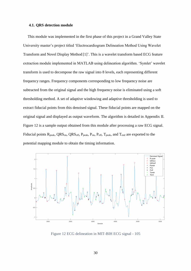
Figure 23 is the signal 114 between 1 minute and 2 minutes of the recording. PVC peak at

1.20minutes can be observed in the figure inside the red box. A more comprehensive

investigation of the PVC detection algorithm will be provided in the Section 5.4.

49

Figure 23 Signal 114 (Upper: Lead V5, Lower: II)

5.3. Mapping

Timing information obtained from the QRS detection module is the input to the mapping

module. A sample of this timing information from 5 different time intervals is listed in Table

4. Sampling frequency of the input signals are 360Hz. The fiducial points from the signal 114

were used to obtain these values.

50

Table 4 Timing information form lead II

Segment Location Time

interval

Time from the input

waveform

(in ms)

P wave Atria 1 100

2 127.8

3 116.7

4 88.9

5 113.9

PQ AV node 1 25

2 22.2

3 16.7

4 5.6

5 5.6

QRS Ventricles 1 130.6

2 130.6

3 116.7

4 147.2

5 133.3

ST Repolarization 1 391.7

2 383.3

3 386.1

4 313.9

5 313.9

51

Figure 24 Output window

Figure 24 is the output window of the implemented visualization system. The top left

image of the output window is the 3D heart envelope mounted with the conduction pathway,

top right portion displays the lead II signal, bottom left image is a cross section of the heart

on which the chest lead potential is mapped and the bottom right portion displays the

corresponding chest lead signal. Simulation of the lead II and the precordial lead are not

designed to execute simultaneously, so the user is only able to see conduction path

information for lead II or the vector amplitude for the precordial lead at a time. Sequential

events involved in the mapping of an ECG complex are as follows:

1. P-wave segment is displayed on both signal display windows (top right and bottom right

portions of the output window). Chest lead potential is mapped on the chest lead vector

at the same time (bottom left of the output window).

52

2. Markers which represents the cardiac potential are moved along the internodal pathways.

3. PQ segment is displayed and the corresponding chest lead potential is mapped on the

chest lead vector.

4. Marker movement is paused at the SA node for tAVnode time.

5. QRS complex is displayed and the corresponding chest lead potential is mapped on the

chest lead vector.

6. Markers are moved along the two Purkinje fibers through bundle of His.

7. ST-segment and the T-wave are displayed and the corresponding chest lead potential is

mapped on the chest lead vector.

8. Potential mapping is paused for tQT time.

A synopsis of this sequence can be observed at the bottom left corner of the output

window. The user can easily understand the simulation procedure with the help of this text

box.

5.3.1. Lead II mapping

Signal 100 is used as the input signal for all the following simulation results in this

section. This signal is 30.06 minutes long and consists of one PVC peak. Figure 25 to Figure

28 are images of the output window during various stages of the simulation. Figure 25 is a P

wave simulation. Blue marker can be observed on the internodal pathways. A fourth marker

can be observed on the Bachmann’s branch in the left atrium.

53

Figure 25 Mapping of the P wave on the conduction pathways

The marker is paused at the SA node during the PQ segment simulation. The marker can

be observed on the conduction pathways (see Figure 26).

Figure 26 Mapping of the PQ segment on the conduction pathways

54

The QRS complex between 25.05min and 25.07min can be observed from the Figure 27.

Corresponding potential movement which is mapped on the Purkinje fiber segment of the

conduction pathway can also be observed on the left.

Figure 27 Mapping of the QRS complex on the conduction pathway

Figure 28 is shows mapping of the ST segment on the conduction pathway. This is the

repolarization time in which heart muscles contracts to squeeze blood outside the ventricle

and then relaxes. Potential mapping is paused for tQT seconds.

55

Figure 28 Mapping of the ST segment on the conduction pathway

5.3.2. Precordial lead mapping

Potential mapping on the chest lead vector, and the signal display take place

simultaneously. Chest lead signal can be observed in the bottom right side of the output

window. Cross sectional image of the thorax along the transverse plane can be observed in

the bottom left side of the same window. Chest lead vector can be observed in the direction of

V5. Potential is mapped along this vector. Signal 100 with V5 lead is used in this section to

demonstrate the chest lead mapping. Figure 29 to Figure 32 shows various stages of the

simulation. Figure 29 shows the potential mapping of a P wave. It can be observed that the

red line is pointing towards the V5 electrode. This line is the lead vector for the

corresponding input signal. A green marker can be observed on this vector which represents

the potential’s position at a given time.

56

Figure 29 Chest lead potential mapping during P wave

Figure 30 demonstrates the potential mapping of an Rpeak. Ideally, the maximum value in a

normal ECG complex will be its Rpeak which is a positive amplitude. As mentioned earlier,

the center of the heart is more negative and the exterior of torso is positive according to the

central limit theorem. Potential’s position can be observed near the V5 electrode.

Figure 30 Chest lead potential mapping during an Rpeak

In Figure 31, a zero potential from the PQ-segment is mapped on the chest lead vector.

Green marker can be seen near the middle portion of the vector.

57

Figure 31 Chest lead potential mapping of a PQ segment

The mapping of a negative amplitude from a PVC peak is demonstrated in the Figure 32.

It can be observed that the green marker corresponding to the potential’s position is near the

center of the heart.

Figure 32 Chest lead potential mapping during a negative amplitude

5.4. PVC detection and mapping

PVCs are identified using the PVC detection algorithm as described in the methods

section. Identified PVCs are labelled using a blue star on the output waveform as shown in

58

the Figure 33. PVC peak at 25.13 minute of the signal 100 is the identified peak in this figure.

An offset of few seconds can be observed in the identified peak as mentioned in the previous

section.

Figure 33 Detected PVC peaks on the signal 100 (Upper: Lead II, Lower: V5)

Only one lead signal is necessary for the algorithm to detect PVC peaks. Lead II signal is

selected for this purpose as in the reference document [19]. Amplitude corresponding to this

point is labelled as a PVC peak on the output waveform of the chest lead. Therefore, chest

lead signal’s output waveform is not used in the evaluation of the PVC peak detection

59

module. Figure 34 and Figure 35 are the lead II output waveforms of the signals 114 and 119

respectively. PVC at 8.31 minute of the signal 114 and uniform PVC peaks at 1.55 minutes of

the signal 119 can be observed in these images.

Figure 34 PVC peaks on signal '114' near 8.31min

60

Figure 35 PVC peaks on signal '119' near 1.55min

Figure 36 shows the mapping of PVC on the heart’s envelope. Color map is changed from

a solid pink to a range of colors during a PVC to draw attention to the aberrant beat. Since the

PVC origin is unpredictable, the red color shows the region in which the potential could be

generated. Other regions are colored differently since they do not generate a PVC. If the

number of identified PVC waves is close to the number of PVCs in a given period of time,

algorithm is robust. Results of this efficiency test is recorded in the Table 5. This test was

performed for all signals in the database with PVC. Results of few signals are recorded in the

Table 5. It is also observed that the system fails to read certain signals within certain time

intervals due to unidentified noise source.

61

Figure 36 PVC mapping

Table 5 PVC peak detection results

Signal Time interval (in

minutes)

Number of PVC

peaks present in this

range

Number of

identified PVC

peaks

100 25 to 26 1 1

114 1 to 5 13 12

116 1 to 5 11 5

119 0 to 5 84 48

200 29 to30 20 19

205 16 to 17 3 2

234 17 to 22 2 2

62

6. Analysis and Discussion

This section discuss the efficiency of the implemented system. Output of the PVC

detection algorithm is compared with the published results17. Three major components

analyzed are the accuracy of the 3D envelope structure, mapping efficiency and the speed.

First component is the cross section of the 3D heart envelope. It can be observed that the

heart is sliced along the mid-plane in order to obtain the cross section. Origin and other two

points where all the vertical lines are merged can be observed from the cross sectional image

of the 3D heart model (see Figure 17). Recall from the literature review section the cardiac

model used for visualization is based on a volumetric reconstruction from MRI slices through

the heart. The horizontal rings or layers represents the boundaries of the MRI slices of the

heart. Among the three points, the top point is the convergence point before the first layer of

the heart model. Bottom point is the apex of the heart. The origin can be observed as blue dot

at the center of the 3D space 2. All three points and the boundary of the 3D space 1 are on the

same plane as seen in the Figure 17. This implies that the heart is sliced along the right plane.

Second component is the mapping efficiency. Factors that determine the efficiency of a

simulation software are its accuracy and speed. While the total simulation time or the

processing time determines the speed of the system, accuracy is determined by the mapping

time of each event (P wave onset and offset, PQ interval, QRS complex duration, and QT

intervals) individually. Among the four ECG segments, mapping time of the P wave onset

and offset, and the QRS complex are the only factors which can influence the total mapping

time. Mapping time of PQ interval and QT interval are direct delay statements. A marker is

paused at each point of an intermodal pathway in order to map P wave onset and offset

segment using tatria. Delay of a fraction of the tatria is applied at each point. This process can

create some additional delays due to various factors including time estimation error, and

63

computational delay of MATLAB. Since the mapping of the signal in the ventricles are

carried out in the same manner, similar delays are anticipated in the mapping of t_ventricles

as well. These additional delays will be referred as ‘mapping delays’ further in this document.

Table 6 is a record of atrial and ventricular mapping time for the three recordings provided in

the Results section. N is the number of ECG components (P-waves for the atrial mapping

delay and QRS complexes for the ventricular mapping delay) present in the given signal

length of the corresponding signal. ∆N is the number of ECG components with a mapping

delay and t∆N is the mapping delay in milliseconds. Maximum t∆N among ∆N ECG

components is only listed in this Table since lesser delays does not and any value in the

analysis of mapping delays.

Table 6 Atrial and Ventricular mapping delays

ECG

componen

t

Signal

length

(in s)

Mapping delay

Signal 100 Signal 119 Signal 234

∆N N Maximum

t∆N (in ms)

∆N N Maximum

t∆N (in ms)

∆N N Maximum

t∆N (in ms)

P-wave

(Atria)

10 3 10 69.5 1 9 62.7 1 13 7.6

20 4 22 62 3 19 29.3 1 28 9.6

30 10 36 60.1 2 30 57.4 0 44 0

40 8 48 31.5 2 42 27.5 0 59 0

50 14 60 82.4 1 52 23.9 1 75 8.2

QRS

Complex

(Ventricle)

10 0 0 0 0 0 0

20 0 0 0 0 0 0

30 0 0 0 0 0 0

40 0 0 0 0 0 0

50 0 0 0 0 0 0

Mapping time of the three signals for five different signal lengths are compared for this

study. Signal 100 and signal 119 are signals with PVCs, while signal 234 does not have a

PVC. Time interval considered for 100 and 119 contains at least one PVC peak. It is observed

that the atrial mapping delay ranges between 5ms and 90ms. Maximum mapping delay was

64

consistently observed at the first P wave. Surprisingly, ventricular mapping time is observed

as zero at every stage of simulation. This segment of the conduction pathways has fewer

points, hence minimum delay. The bundle of His and Purkinje fibers are the only components

of the conduction pathway in the ventricular region. These are designed using fewer points

due to a more linear structure as compared to the internodal pathways. Hence, fewer

iterations are required to move the marker along this structure. In addition, unlike internodal

pathways with three paths and a Bachmann’s branch, Purkinje fiber only has two paths. This

makes it less computationally intensive to move the marker.

Third component to analyze is the PVC detection schema. Signals 100, 114, 116, and 119

were used in the reference research (Chang’s model [19]) to test the algorithm. Response of

the system for these same signals are analyzed here to verify the efficiency of the PVC

detection algorithm. Figure 37 to Figure 40 are the output waveforms of 100, 114, 116 and

119 respectively. Characteristics of these signals were available from the Physionet database

[21] [22].

65

Figure 37 Signal 100 - Lead II (First 5 minutes)

Figure 37 is an image of the first 5 minutes of the signal 100. According to the signal

properties, no PVC is present in this segment of signal 100. PVC peaks cannot be observed in

this output waveform as well. This implies that the PVC detection module was successful in

discarding non-PVC peaks for this input signal.

66

Figure 38 Signal 114 - Lead II (First 5 minutes)

13 PVC peaks are present in the first 5 minutes of the signal 114. It can be observed from

the Figure 38 that the system was able to detect all PVC peaks. However, in certain cases if

the last Rpeak is a PVC and if the whole PQRST information of that particular ECG complex

is not available within the signal length, the algorithm will not identify it as a PVC. These

peak can be detected if plotted separately with a wider signal length. The undetected PVC

peaks will bring down the success rate of the PVC detection algorithm. This implies that the

signal length can influence the efficiency of the PVC detection module. Only parameter

changed to detect the signal is the number of Rpeaks. Since number of Rpeaks changed, average

RRI also changed. This leads to more accurate detection of the PVC peaks. PVC detection

results obtained for the other two input signals can be observed from the Figure 39 and Figure

40. From the Figure 40 it can be observed that the algorithm failed to detect a considerable

amount of PVC peaks for the signal 119. It can also be observed that the number of PVC

peaks were really high during this range. Therefore, the average RRI of the total signal length

67

will skew towards the average RRI of the PVC peaks. Thus, the algorithm detects only those

signals which are higher than this skewed average RRI as PVC peaks. This is a limitation of

the first threshold used in the implemented algorithm.

Figure 39 Signal 116 - Lead II (First 5 minutes)

68

Figure 40 Signal 119 - Lead II (First 5 minutes)

Tables 7, 8, 9, 10, and 11 are the specificity and sensitivity analysis of the PVC detection

algorithm for any 5 minutes of these four signals in which at least a PVC peak is present. If a

PVC peak is expected and detected, it is counted as true-positive, if a PVC is not expected

but detected, it is a false-positive, if a PVC peak is expected but not detected, it is a false-

negative and if a PVC peak is not expected and not detected, it is a true-negative. The

accuracy, specificity and sensitivity of the algorithm can be obtained using the equations 6.1

to 6.3. Figure 41 shows the true positive analysis chart. Table 7 to Table 10 can be interpreted

using this figure.

69

Figure 41 True positive rate analysis chart

Table 7 True positive analysis on signal 100

Condition positive Condition negative

PVC detected 1 0

PVC not detected 0 369

Table 8 True positive analysis on signal 114

Condition positive Condition negative

PVC detected 12 1

PVC not detected 0 264

70

Table 9 True positive analysis on signal 116

Condition positive Condition negative

PVC detected 5 5

PVC not detected 3 375

Table 10 True positive analysis on signal 119

Condition positive Condition negative

PVC detected 37 41

PVC not detected 9 241

Sensitivity,

Sensitivity = ∑ True positive

∑ Condition positive X 100 (6.1)

Specificity,

Specificity = ∑ True negative

∑ Condition negative X 100 (6.2)

Accuracy,

Accuracy = ∑ True positive+∑ True negative

∑ Condition positive+∑ Condition negative X 100 (6.3)

71

Table 11 PVC detection algorithm efficiency study

Signal This research Chang’s model [19]

Specificity Sensitivity Accuracy Accuracy

100 100% 100% 100% 100%

114 100% 99.62% 99.64% Not Available

116 62.6% 98.68% 97.94% Mean accuracy of 116 and

119 is 72.96% 119 80.43% 85.46% 84.75%

Average 95.58% 86.48%

The specificity and sensitivity calculated for these four signals are listed in the Table 11,

along with the accuracy values published in Chang’s research [19]. It can be observed that the

average accuracy of the PVC detection algorithm implemented in this system is 9% more

than that of the Chang’s model. Combination of the thresholds to filter non-PVC peaks were

altered in the design implemented for this thesis. In Chang’’s model, third threshold is only

applied if the second threshold fails to detect a PVC. However, in the proposed design,

second and third thresholds are applied even if either one fails to detect a PVC. Therefore,

there is more probability to obtain more true-positives. The increase in the average accuracy

proves that the changes made to the algorithms improved the performance. However, PVC

detection algorithm tends to change its performance with varying signal length. The system

detects PVCs more accurately when the signal length is smaller. The factor influencing this

tendency is the first threshold. As mentioned in the methods section, the first threshold is an

average value of Rpeak to Rpeak intervals. When only few samples are present to compare with

this threshold, peaks will remain unique. Thus it can be easily identified. For example, PVC

peaks were identified more accurately when a shorter signal range was selected within the

first 5 minutes of the signal 119.

72

7. Conclusion

A tool for 3D visualization of cardiac excitation was implemented using MATLAB as a

second phase of the educational tool development project during the course of this thesis.

Main features focused in this implementation were a 3D heart model, conduction pathway

identification, accurate timing information, and PVC detection. Timing information was

obtained from the wavelet transform based QRS detection module implemented in the first

phase1. An MRI reconstructed 3D heart was used to develop suitable heart envelope and the

conduction pathway.

The 3D heart was sliced along the frontal plane and SA node, AV node and conduction

pathway components were defined for mapping purpose using co-ordinate functions and 3D

spline functions. Timing information obtained from the QRS detection module was used to

move markers along the internodal pathways and Purkinje fiber. It is observed that the atrial

mapping delay was in the range of 5ms to 83ms. This is a small fraction compared to the total

simulation time. Ventricular mapping delay was observed as zero due to the lighter structure

of the ventricular segments of the conduction pathways. One chest lead was used to

determine the location of the potential from a top view or a cross sectional view along the

transverse plane. Even though the total simulation time was affected by several external

factors, it is observed that the change in this time is linear and correlated with the simulation

speed scaling factor as expected.

Two additional thresholds other than the first average Rpeak to Rpeak time interval threshold

were used to implement the PVC detection module: sum of trough and sum of Rpeak with

minimum. PVCs with wider Rpeak to Rpeak interval were detected using sum of trough

threshold and PVCs with unique amplitude features were detected using the sum of Rpeak with

minimum threshold. Efficiency of this detection algorithm is compared with the Chang’s

73

model which uses same thresholds in different combination to detect PVCs. Signals 100, 114,

116, and 119 were used to detect the PVC peaks as in Chang’s model. Even though the

success rate in detecting the PVC peaks of the first two signals were high, the success rate

was comparatively low in the other two signals. It is also observed that the success rate

increases with shorter signal length. An adaptive average RRI as threshold 1 would help in

solving this issue.

The implemented 3D visualization system was successful in mapping the potential on the

defined conduction pathway. The PVC detection module was also successful in

distinguishing between a PVC and a non PVC wave with nearly 95% accuracy. However,

total simulation time is affected by several external factors like computational delays and

computer specification limitations. More chest lead inputs can determine more accurate

position of the potential on the transverse plane. This is desired in the future work of this

project.

74

8. Appendix I – Source code

8.1. GUI

%%%%%%%%%%%%%%%%%%%%%%%%%%%%%%%%%%%%%%%%%%%%%%%%%%%%%%%%%%%%%%%%%%%%%%%%%%% % GUI_3D_Visualization_Input() % % Author : Pranav Sreedharan Veliyara % Advisor : Dr. Samhita Rhodes % Project : Master's thesis at Grand Valley State University % Thesis title : Visualization of the cardiac excitation and PVC % arrhtythmia on a 3D heart model % Code version : 1.0 % Published year: 2017 % % Description : This file consists of GUI main function and all the % call back functions for the GUI. % % Note : This file is autogenerated from the MATLAB GUI GUIDE. %%%%%%%%%%%%%%%%%%%%%%%%%%%%%%%%%%%%%%%%%%%%%%%%%%%%%%%%%%%%%%%%%%%%%%%%%%%

function varargout = GUI_3D_Visualization_Input(varargin) %GUI_3D_VISUALIZATION_INPUT M-file for GUI_3D_Visualization_Input.fig % GUI_3D_VISUALIZATION_INPUT, by itself, creates a new % GUI_3D_VISUALIZATION_INPUT or raises the existing singleton*. % % H = GUI_3D_VISUALIZATION_INPUT returns the handle to a new % GUI_3D_VISUALIZATION_INPUT or the handle to the existing singleton*. % % GUI_3D_VISUALIZATION_INPUT('Property','Value',...) creates a new % GUI_3D_VISUALIZATION_INPUT using the given property value pairs. % Unrecognized properties are passed via varargin to % GUI_3D_Visualization_Input_OpeningFcn. This calling syntax produces % a warning when there is an existing singleton*. % % GUI_3D_VISUALIZATION_INPUT('CALLBACK') and % GUI_3D_VISUALIZATION_INPUT('CALLBACK',hObject,...) call the local % function named CALLBACK in GUI_3D_VISUALIZATION_INPUT.M with the % given input arguments. % % *See GUI Options on GUIDE's Tools menu. Choose "GUI allows only one % instance to run (singleton)". % % See also: GUIDE, GUIDATA, GUIHANDLES

% Edit the above text to modify the response to help % GUI_3D_Visualization_Input

% Last Modified by GUIDE v2.5 23-Apr-2017 01:55:02

% Begin initialization code - DO NOT EDIT gui_Singleton = 1; gui_State = struct('gui_Name', mfilename, ... 'gui_Singleton', gui_Singleton, ... 'gui_OpeningFcn',

@GUI_3D_Visualization_Input_OpeningFcn, ...

75

'gui_OutputFcn', @GUI_3D_Visualization_Input_OutputFcn,

... 'gui_LayoutFcn', [], ... 'gui_Callback', []); if nargin && ischar(varargin1) gui_State.gui_Callback = str2func(varargin1); end

if nargout [varargout1:nargout] = gui_mainfcn(gui_State, varargin:); else gui_mainfcn(gui_State, varargin:); end % End initialization code - DO NOT EDIT

% --- Executes just before GUI_3D_Visualization_Input is made visible. function GUI_3D_Visualization_Input_OpeningFcn(hObject, eventdata, ... handles, varargin) % This function has no output args, see OutputFcn. hObject handle to % figure eventdata reserved - to be defined in a future version of MATLAB % handles structure with handles and user data (see GUIDATA) varargin % unrecognized PropertyName/PropertyValue pairs from the % command line (see VARARGIN)

% Choose default command line output for GUI_3D_Visualization_Input handles.output = hObject;

% Update handles structure guidata(hObject, handles);

% UIWAIT makes GUI_3D_Visualization_Input wait for user response (see % UIRESUME) uiwait(handles.figure1);

% --- Outputs from this function are returned to the command line. function varargout = GUI_3D_Visualization_Input_OutputFcn(hObject, ... eventdata, handles) % varargout cell array for returning output args (see VARARGOUT); hObject % handle to figure eventdata reserved - to be defined in a future version % of MATLAB handles structure with handles and user data (see GUIDATA)

% Get default command line output from handles structure varargout1 = handles.output;

function StartTime_Callback(hObject, eventdata, handles) % hObject handle to StartTime (see GCBO) eventdata reserved - to be % defined in a future version of MATLAB handles structure with handles % and user data (see GUIDATA) Start_timeVar = str2num(get(handles.StartTime,'String')); setappdata(0,'Start_time',Start_timeVar);

% Hints: get(hObject,'String') returns contents of StartTime as text % str2double(get(hObject,'String')) returns contents of StartTime as % a double

76

% --- Executes during object creation, after setting all properties. function StartTime_CreateFcn(hObject, eventdata, handles) % hObject handle to StartTime (see GCBO) eventdata reserved - to be % defined in a future version of MATLAB handles empty - handles not % created until after all CreateFcns called

% Hint: edit controls usually have a white background on Windows. % See ISPC and COMPUTER. if ispc && isequal(get(hObject,'BackgroundColor'), ... get(0,'defaultUicontrolBackgroundColor')) set(hObject,'BackgroundColor','white'); end

function AddTime_Callback(hObject, eventdata, handles) % hObject handle to AddTime (see GCBO) eventdata reserved - to be % defined in a future version of MATLAB handles structure with handles % and user data (see GUIDATA) Add_timeVar = str2num(get(handles.AddTime,'String')); Start_timeTe=getappdata(0,'Start_time'); fs=360; Start_pointVar=Start_timeTe*fs*60; Add_pointVar=Add_timeVar*fs*60; End_pointVar=Start_pointVar+Add_pointVar; setappdata(0,'Start_point',Start_pointVar); setappdata(0,'End_point',End_pointVar); % setappdata(0,'Add_time',Add_time);

% Hints: get(hObject,'String') returns contents of AddTime as text % str2double(get(hObject,'String')) returns contents of AddTime as a % double

% --- Executes during object creation, after setting all properties. function AddTime_CreateFcn(hObject, eventdata, handles) % hObject handle to AddTime (see GCBO) eventdata reserved - to be % defined in a future version of MATLAB handles empty - handles not % created until after all CreateFcns called

% Hint: edit controls usually have a white background on Windows. % See ISPC and COMPUTER. if ispc && isequal(get(hObject,'BackgroundColor'), ... get(0,'defaultUicontrolBackgroundColor')) set(hObject,'BackgroundColor','white'); end

% --- Executes on selection change in LeadIIpopup. function LeadIIpopup_Callback(hObject, eventdata, handles) % hObject handle to LeadIIpopup (see GCBO) eventdata reserved - to be % defined in a future version of MATLAB handles structure with handles % and user data (see GUIDATA) LeadIIpopupContents=cellstr(get(hObject,'String')); InputFileVar=LeadIIpopupContentsget(hObject,'Value'); if (strcmp(InputFileVar,'mitdb/114')) % If 114 is selected,

77

% this condition checks the status nVar=2; % and automatically assigns limb % lead to channel 1 and the available vVar=1; % precordial lead to chnnel 2. else nVar=1; vVar=2; end setappdata(0,'n',nVar); setappdata(0,'v',vVar); setappdata(0,'InputFile',InputFileVar);

% Hints: contents = cellstr(get(hObject,'String')) returns LeadIIpopup % contents as cell array % contentsget(hObject,'Value') returns selected item from % LeadIIpopup

% --- Executes during object creation, after setting all properties. function LeadIIpopup_CreateFcn(hObject, eventdata, handles) % hObject handle to LeadIIpopup (see GCBO) eventdata reserved - to be % defined in a future version of MATLAB handles empty - handles not % created until after all CreateFcns called

% Hint: popupmenu controls usually have a white background on Windows. % See ISPC and COMPUTER. if ispc && isequal(get(hObject,'BackgroundColor'), ... get(0,'defaultUicontrolBackgroundColor')) set(hObject,'BackgroundColor','white'); end

% --- Executes on selection change in Precordialpopup. function Precordialpopup_Callback(hObject, eventdata, handles) % hObject handle to Precordialpopup (see GCBO) eventdata reserved - to % be defined in a future version of MATLAB handles structure with % handles and user data (see GUIDATA) PrecordialpopupContents = cellstr(get(hObject,'String')); leadVar = PrecordialpopupContentsget(hObject,'Value'); if (strcmp(leadVar,'V1')) leadV=1; elseif (strcmp(leadVar,'V2')) leadV=2; elseif (strcmp(leadVar,'V3')) leadV=3; elseif (strcmp(leadVar,'V4')) leadV=4; elseif (strcmp(leadVar,'V5')) leadV=5; elseif (strcmp(leadVar,'V6')) leadV=6; else leadV=1; end setappdata(0,'lead',leadV);

% Hints: contents = cellstr(get(hObject,'String')) returns Precordialpopup % contents as cell array % contentsget(hObject,'Value') returns selected item from

78

% Precordialpopup

% --- Executes during object creation, after setting all properties. function Precordialpopup_CreateFcn(hObject, eventdata, handles) % hObject handle to Precordialpopup (see GCBO) eventdata reserved - to % be defined in a future version of MATLAB handles empty - handles not % created until after all CreateFcns called

% Hint: popupmenu controls usually have a white background on Windows. % See ISPC and COMPUTER. if ispc && isequal(get(hObject,'BackgroundColor'), ... get(0,'defaultUicontrolBackgroundColor')) set(hObject,'BackgroundColor','white'); end

% --- Executes on selection change in scale. function scale_Callback(hObject, eventdata, handles) % hObject handle to scale (see GCBO) eventdata reserved - to be defined % in a future version of MATLAB handles structure with handles and user % data (see GUIDATA) ScaleContents=cellstr(get(hObject,'String')); scaleVar=ScaleContentsget(hObject,'Value'); scaleVar=str2num(scaleVar); setappdata(0,'scale',scaleVar);

% Hints: contents = cellstr(get(hObject,'String')) returns scale contents % as cell array % contentsget(hObject,'Value') returns selected item from scale

% --- Executes during object creation, after setting all properties. function scale_CreateFcn(hObject, eventdata, handles) % hObject handle to scale (see GCBO) eventdata reserved - to be defined % in a future version of MATLAB handles empty - handles not created % until after all CreateFcns called

% Hint: popupmenu controls usually have a white background on Windows. % See ISPC and COMPUTER. if ispc && isequal(get(hObject,'BackgroundColor'), ... get(0,'defaultUicontrolBackgroundColor')) set(hObject,'BackgroundColor','white'); end

% --- Executes on button press in RunButton. function RunButton_Callback(hObject, eventdata, handles) % hObject handle to RunButton (see GCBO) eventdata reserved - to be % defined in a future version of MATLAB handles structure with handles % and user data (see GUIDATA) InputFile=getappdata(0,'InputFile'); n=getappdata(0,'n'); v=getappdata(0,'v'); lead=getappdata(0,'lead'); Start_point=getappdata(0,'Start_point'); End_point=getappdata(0,'End_point'); scale=getappdata(0,'scale');

79

Conduction3D(InputFile,n,v,lead,Start_point,End_point,scale); guidata(hObject, handles);

8.2. Timing information

%%%%%%%%%%%%%%%%%%%%%%%%%%%%%%%%%%%%%%%%%%%%%%%%%%%%%%%%%%%%%%%%%%%%%%%%%%% % Timing_Function() % % Author : Pranav Sreedharan Veliyara % Advisor : Dr. Samhita Rhodes % Project : Master's thesis at Grand Valley State University % Thesis title : Visualization of the cardiac excitation and PVC % arrhtythmia on a 3D heart model % Code version : 1.0 % Published year: 2017 % % Description : This function is a bridge between the main function % andthe sub-functions those obtain fiducial points on % the input signal. The fiducial points obtained from % the sub-functions are marked on the input signal here. % % Input : InputFile - (string) Signal name as published in the % MIT-BIH arrhythmia database. % fs - Sampling frequency % n, v - These variable internally assigns % appropriate channel to lead II and the % precordial lead signals. Channel 1 always % has the lead II signal and channel 2 % always contains the precordial signal. % lead - Precordial lead selection. % Start_point, End_point - X-coordinate information of % the first sample and the last sample of the input % signal. % % Output : ECG,ECGv - Raw lead II and precordial signals % respectively. % sig_denoised,sigv_denoised - Denoised lead II and the % precordial signals respectively. % tm - Time variabe that saves the duration of the % input signal. % Rpeak,QRSon,QRSoff,Ppeak,Pon,Poff,Tpeak,Tend - Fiducial % points on the lead II. % vRpk,vRon,vRoff - Fiducial points on the precordial % lead. % PVCMat - Matrix that saves the position and amplidude % information of the detected PVC peaks. % % Note : This function calls the components of the QRS detection % module developed by Mr. Eric VanMiddendorp, % in the first phase of this project for his master's % thesis (Reference [1]). Source code for those % components are not available to the reader from this % thesis document. These functions are labelled (in % comment nearby the function call) as EV. %%%%%%%%%%%%%%%%%%%%%%%%%%%%%%%%%%%%%%%%%%%%%%%%%%%%%%%%%%%%%%%%%%%%%%%%%%%

function [ECG,ECGv,sig_denoised,sigv_denoised,tm,Rpeak,QRSon,QRSoff,... Ppeak,Pon,Poff,Tpeak,Tend,PVCMat,vRpk,vRon,vRoff]=...

80

Timing_Function(InputFile,n,v,fs,Start_point,End_point,lead)

[tm,ECG]=rdsamp(InputFile,n); %222 [tm,ECGv]=rdsamp(InputFile,v);

% 1min is equal to 21600 @360 fs (Sampling frequency) sig = ECG(Start_point:End_point); %114,119

sigv = ECGv(Start_point:End_point);

wname = 'sym5';

%zero-mean the data sig = sig-mean(sig); sigv = sigv-mean(sigv);

%Remove baseline wander and denoise the signal Perform a multilevel wavelet %decomposition (Level 8, sym5 wavelet, plot) [sig_denoised,C,L] = WaveletDenoise(sig,wname,8,0); [sigv_denoised,Cv,Lv] = WaveletDenoise(sigv,wname,8,0);

%Center signal sig_denoised= sig_denoised+0.05; sigv_denoised= sigv_denoised+0.05;

%% Lead II signal %Find the R peaks in the denoised signal Rpeak = R_PeakDetect_Final(sig_denoised,fs,0); % EV

%QRS-on detection QRSon = QRS_OnDetect(sig_denoised,Rpeak,fs,0); % EV

%QRS-off detection QRSoff = QRS_OffDetect(sig_denoised,Rpeak,fs,0); % EV

%P wave detection [Ppeak,Pon,Poff] = P_WaveDetect_Final(sig_denoised,Rpeak,QRSon,fs,0); % EV

%T wave detection [Tpeak,Tend]=T_WaveDetect_imageproc(sig_denoised,Rpeak,QRSoff,QRSon,fs,0); % EV

%% Precordial lead Signal %Find the R peaks in the denoised signal vRpk = R_PeakDetect_Final(sigv_denoised,fs,0); % EV

%QRS-on detection vRon = QRS_OnDetect(sigv_denoised,vRpk,fs,0); % EV

%QRS-off detection vRoff = QRS_OffDetect(sigv_denoised,vRpk,fs,0); % EV

% PVC detection module [PVCMat,PVCMatv]=PVC_Detect(sig_denoised, sigv_denoised, fs, Rpeak, vRpk);

%% Plotting the location of the fudicial points plot_data = 1; sig_length=Start_point/(fs*60):1/(fs*60):End_point/(fs*60);

81

if (plot_data) figure (1); % Plots the lead II signal and marks the fiducial points % on this signal here. plot(sig_length,sig_denoised);hold on; plot((Start_point+Rpeak(:,2))/(fs*60),Rpeak(:,1),'ro','MarkerSize',6); hold on; plot((Start_point+QRSon(:,2))/(fs*60),QRSon(:,1),'r^','MarkerSize',6); hold on; plot((Start_point+QRSoff(:,2))/(fs*60),QRSoff(:,1),... 'r^','MarkerSize',6); hold on; plot((Start_point+Ppeak(:,2))/(fs*60),Ppeak(:,1),'ko','MarkerSize',6); hold on; plot((Start_point+Pon(:,2))/(fs*60),Pon(:,1),'k*','MarkerSize',6); hold on; plot((Start_point+Poff(:,2))/(fs*60),Poff(:,1),'k*','MarkerSize',6); hold on; plot((Start_point+Tpeak(:,2))/(fs*60),Tpeak(:,1),'go','MarkerSize',6); hold on; plot((Start_point+Tend(:,2))/(fs*60),Tend(:,1),'g*','MarkerSize',6); hold on; plot((Start_point+PVCMat(2:end,2))/(fs*60),PVCMat(2:end,1),... 'b*','MarkerSize',6); xlabel('Time (in minutes)');ylabel('Amplitude (in mV)'); title('Input Signal - Lead II'); h_leg = legend('Denoised Signal','R-peak','QRSon','QRSoff','Ppeak',... 'Pon','Poff','Tpeak','Tend','PVC peak'); set(h_leg,'FontSize',12); end

figure (2); % Plots the precordial lead signal and marks the fiducial % points on this signal here. plot(sig_length,sigv_denoised);hold on; plot((Start_point+vRpk(:,2))/(fs*60),vRpk(:,1),'ro','MarkerSize',6); hold on; plot((Start_point+vRon(:,2))/(fs*60),vRon(:,1),'g^','MarkerSize',6); hold on; plot((Start_point+vRoff(:,2))/(fs*60),vRoff(:,1),'r^','MarkerSize',6); hold on; plot((Start_point+PVCMatv(2:end,2))/(fs*60),PVCMatv(2:end,1),... 'b*','MarkerSize',6); xlabel('Time (in minutes)');ylabel('Amplitude (in mV)'); title(['Input Signal - Precordial Lead V',num2str(lead)]); h_leg = legend('Denoised Signal','R-peak','QRSon','QRSoff','PVC peak'); set(h_leg,'FontSize',12);

end

82

8.3. Heart envelope

%%%%%%%%%%%%%%%%%%%%%%%%%%%%%%%%%%%%%%%%%%%%%%%%%%%%%%%%%%%%%%%%%%%%%%%%%%% % SM_HeartEnvelope() % % Author : Pranav Sreedharan Veliyara % Advisor : Dr. Samhita Rhodes % Project : Master's thesis at Grand Valley State University % Thesis title : Visualization of the cardiac excitation and PVC % arrhtythmia on a 3D heart model % Code version : 1.0 % Published year: 2017 % % Description : This function imports the 3D heart envelope mentioned % in the reference [20] and extracts only one half % section along the frontal plane. % % Note : This function is a modified code of a code published % in MathWorks website. Few lines of this function and % the function named 'povorot3()' are taken from the % reference [20]. Lines of code those are not modified % are grouped under SM tag here. Author details of those % lines of code is as given below: % Sergei Malchenko, University of Tartu, 2002, Vers. 1.0 %%%%%%%%%%%%%%%%%%%%%%%%%%%%%%%%%%%%%%%%%%%%%%%%%%%%%%%%%%%%%%%%%%%%%%%%%%%

function SM_HeartEnvelope() %% SM prop=35; Z_sdvig=3; mastbZ=30; xo=0/prop; yo=7/prop; zo=-Z_sdvig.*mastbZ/prop;

load('heart.mat');

Tper=0.77; % Heart period, in seconds N=20; % Desired number of frames per cardiac cycle

THETA=-pi:pi./30:pi; % Azimuth grid PHI=-pi./2:pi./30:pi./2; % Elevation grid TIME=0:Tper/N:Tper; % Time grid

Rvalues = fnval(heartsurf,THETA,PHI,TIME); set(gcf,'Position',[1 29 400 200]);

for Time=1:size(Rvalues,3) Rs(:,:,Time)=Rvalues(:,:,Time).'; end Rvalues=Rs; clear Rs;

M=moviein(size(heartsurf,1)); [THETA,PHI] = meshgrid(THETA,PHI);

% for Time=1:size(Rvalues,3)

83

Time=1; a=size(Rvalues(:,:,Time)); Rvalues_tt=(Rvalues(:,:,Time)); Rvalues_t=Rvalues_tt(:).'; THETA_t=(THETA(:)).'; PHI_t=(PHI(:)).'; Rvalues_tt=[]; [XX,YY,ZZ]=sph2cart(THETA_t,PHI_t,Rvalues_t); Object=[XX+xo;YY+yo;ZZ+zo]; Object=[XX;YY;ZZ]; % povorot3 - function, used for setting preferred direction for new % Z-axis direction: NewObject=povorot3(Object);

%% Following lines are modified for this thesis and adapted from the % reference [20].

XMx=[ones(31,31),zeros(31,30)]; % Zero matrix equalent to the half section of the % heart envelope.

XX=reshape(NewObject(1,:),a).*XMx; % Extracting one half of the YY=reshape(NewObject(2,:),a).*XMx; % 3D envelope by multiplying with ZZ=reshape(NewObject(3,:),a).*XMx; % the zero matrix.

XX=XX(1:31,1:31); YY=YY(1:31,1:31); ZZ=ZZ(1:31,1:31);

XX=XX.*cos(pi/3.7)+YY.*sin(pi/3.7); % Defining the coordinates in the YY=-XX.*sin(pi/3.7)+YY.*cos(pi/3.7); % cartesian coordinate system.

h=surf(XX,YY,ZZ); % Plotting the derived heart model

% Display parameters settings. hold on grid on box on set(gcf,'Color',[1 1 1]); set(h,'FaceLighting','phong','EdgeColor',[1 1 1]); set(gcf,'Renderer','zbuffer') colormap (pink) caxis([-11.5,21.5]) set(gca,'XDir','reverse') axis square

camzoom(1.5) camproj perspective

xlabel('X(cm)'); ylabel('Y(cm)'); zlabel('Z(cm)','Rotation',0); title('Human Heart - 3D Envelope','FontSize',16);

axis([-8 7 -4 3 -7.5 7.5]); view(158,6);

end

84

8.4. PVC detection

%%%%%%%%%%%%%%%%%%%%%%%%%%%%%%%%%%%%%%%%%%%%%%%%%%%%%%%%%%%%%%%%%%%%%%%%%%% % PVC_Detect() % % Author : Pranav Sreedharan Veliyara % Advisor : Dr. Samhita Rhodes % Project : Master's thesis at Grand Valley State University % Thesis title : Visualization of the cardiac excitation and PVC % arrhtythmia on a 3D heart model % Code version : 1.0 % Published year: 2017 % % Description : This function is a bridge between the main function % and sub-functions those obtain fiducial points on % the input signal. The fiducial points obtained from % the subfunctions are marked on the input signal here. % % Input : sig_denoised,sigv_denoised - Denoised lead II and the % precordial signals respectively. % fs - Sampling frequency % Rpeak,vRpk- R peaks detectected on the lead II signal % and the selected precordial signal % respectively. % % Output : PVCMat, PVCMatv - Matrix that saves the position and % amplidude information of the detected % PVC peaks from the lead II signal and from % the selected precordial lead signal % respectively. % % Note : RRI is R-peak to R-peak interval. %%%%%%%%%%%%%%%%%%%%%%%%%%%%%%%%%%%%%%%%%%%%%%%%%%%%%%%%%%%%%%%%%%%%%%%%%%%

function [PVCMat,PVCMatv] = PVC_Detect(sig_denoised, sigv_denoised, ... fs, Rpeak, vRpk)

% % PVC Detection PVCx=0;PVCy=0; % Variables to save the time and the amplitude PVCxv=0;PVCyv=0; % information of the detected PVC peaks.

PVCpk=0; % Variable to save the index of the detected % PVC peak.

PVC_Thr=1*((Rpeak(end,2)-Rpeak(1,2))/(length(Rpeak)-1)); % First threshold. Average RRI.

for j=2:(length(Rpeak)) % Checking every R peaks for a PVC condition.

sum_tr=0; % Variable for sum of trough (second threshold).

RR_min=0; % Variable to store the position of the point % with mimimum amplitude withi the current RRI.

diff=0; % Variable to store the third threshold.

if (((Rpeak(j,2)-Rpeak(j-1,2))>1*PVC_Thr))

85

% Condition for the first threshold. for n=0:50 sum_tr=sum_tr+sig_denoised(Rpeak(j,2)+n); % Second threshold. Sum of trough. end if (sum_tr<0) % Condition for the second threshold. PVCy=[PVCy;Rpeak(j-1,2)]; % Saving the time and amplitude PVCx=[PVCx;Rpeak(j-1,1)]; % points of the detected PVC peak. PVCyv=[PVCyv;vRpk(j-1,2)]; PVCxv=[PVCxv;vRpk(j-1,1)]; PVCpk=[PVCpk;j-1]; end

RR_min=min(sig_denoised(Rpeak(j-1,2):Rpeak(j,2))); % Mimimum value within the RRI. diff=RR_min+Rpeak(j-1,1); % Third threshold. Sum of R-peak with minimum.

if (diff<0) % Condition for the third threshold. PVCy=[PVCy;Rpeak(j-1,2)]; % Saving the time and amplitude PVCx=[PVCx;Rpeak(j-1,1)]; % points of the detected PVC peak. PVCyv=[PVCyv;vRpk(j-1,2)]; PVCxv=[PVCxv;vRpk(j-1,1)]; PVCpk=[PVCpk;j-1]; end end end

PVCMat=[PVCx, PVCy, PVCpk]; % Array of the detected PVC peaks (Lead II). PVCMatv=[PVCxv, PVCyv,PVCpk]; % Array of the detected PVC peaks (Precordial lead).

end

8.5. Precordial lead vector

%%%%%%%%%%%%%%%%%%%%%%%%%%%%%%%%%%%%%%%%%%%%%%%%%%%%%%%%%%%%%%%%%%%%%%%%%%% % PlotVector() % % Author : Pranav Sreedharan Veliyara % Advisor : Dr. Samhita Rhodes % Project : Master's thesis at Grand Valley State University % Thesis title : Visualization of the cardiac excitation and PVC % arrhtythmia on a 3D heart model % Code version : 1.0 % Published year: 2017 % % Description : This function draws the cardiac vector along the % transverse plane and distributes the amplitude % along this vector based on the histogram of the % selected precordial signal. Based on the distribution % algorithm implemented here, a lookup table is generated % with the amplitude and reference points on the vector. % This lookup table is used in the % 'Conduction3D()' function to map the cardiac potentias % on the vector.

86

% % Input : sigv_denoised - Denoised precordial signal. % lead - Precordial lead selection. % axis_im_v- Figure handler for the transverse plane. % % Output : VectorMat- Matrix containing the lookup table with % position and the amplitude information % required for the cardiac vector. % curve11 - Vector along the selected precordial lead. % %%%%%%%%%%%%%%%%%%%%%%%%%%%%%%%%%%%%%%%%%%%%%%%%%%%%%%%%%%%%%%%%%%%%%%%%%%%

function [VectorMat, curve11] = PlotVector(sigv_denoised, lead, axis_im_v) lx=300; % coordinates of the center of the heart ly=220; if(lead==1) % If precordial lead 1 is selected ux=246; % x co-ordinate of the upper point VectorV1 = [ux,90; 273,155; lx,ly]; % [upper point(x,y), mid point(x,y), lower point(x,y)] % Points to draw the cardiac vector along lead 1.

elseif(lead==2) % If precordial lead 2 is selected ux=320; VectorV1 = [ux,90; 310,155; lx,ly]; elseif(lead==3) % If precordial lead 3 is selected ux=380; VectorV1 = [ux,90; 340,155; lx,ly]; elseif(lead==4) % If precordial lead 4 is selected ux=450; VectorV1 = [ux,110; 375,165; lx,ly]; elseif(lead==5) % If precordial lead 5 is selected ux=480; VectorV1 = [ux,176; 390,198; lx,ly]; elseif(lead==6) % If precordial lead 6 is selected ux=500; VectorV1 = [ux,256; 400,238; lx,ly]; end

VectorV1x=VectorV1(:,1);VectorV1y=VectorV1(:,2); % Saving coordinates to a variable

imv=imread('Precordial_leads.png'); % Radiographic image of the cross sectional view % of the torso (transverse plane). imshow(imv, 'Parent', axis_im_v); title('Transverse plane and precordial leads','FontSize',16); xlabel('x'); ylabel('y'); hold on

% Drawing the cardiac vector along the selected lead on the transverse % plane. [curve11] = fit(VectorV1(:,1),VectorV1(:,2),'poly2'); plot(curve11,'-r', VectorV1(:,1),VectorV1(:,2)); hold on; legend('off')

% Defining thesholds for the distribution of the amplitudes along the % selected vector. numberOfBins = 200; % Bins for the histogram. Higher the bins more

87

% the classes. Thus smooth movement of the points % along the vector. [counts, binValues] = hist(sigv_denoised,numberOfBins); % Histogram to find the amplitude disptribution pattern.

normalizedCounts = 100 * counts / sum(counts); % Defining class width for the amplitude distribution.

histMat=[normalizedCounts; binValues]';

yv=sigv_denoised; % To avoid long names in the function parameter list.

lenA=length(histMat); brPt=0; % Break point (transition from negative to positive amplitude) for i=2:1:lenA % Finding the point where the amplitude changes form negative to % positive if (((sign(histMat(i-1,end))==-1)||(sign(histMat(i-1,end))==0)) ... &&(sign(histMat(i,end)))==1) brPt=i-1; else brPt=brPt; end end

x2=zeros(1,lenA)'; % Variable to store the points in the class from the histogram mid=min(lx,ux)+abs(ux-lx)/2; x2(brPt)=mid; x2(1)=lx; x2(lenA)=ux;

divn1=abs(lx-mid)/50; % Distribution width. divn2=abs(ux-mid)/50;

% ux and lx are different for different leads. This conditions will check % whether the ux or lx is the largest value and determines between % upcounter or downcounter. if(min(lx,ux)==lx) divn1=divn1; divn2=divn2; else divn1=-divn1; divn2=-divn2; end

% Mapping of the points along the vector is performed in two steps. In the % first step, certain values are assigned for the amplitudes till the break % point which helps in the mapping of the points till the break point on % one half of the vector. The remaining points are mapped in the second % step. The values assigned in these steps are a constant units apart and % within the range of lx to ux. This two step processhelps in choosing % suitable class width if the distribution of the amplitudes is sporadic % in a different database. This is a provision for the future code % development.

% Mapping the points till the break point on the vector. divn1s=0; counter1=0;

88

for i=2:brPt-1 if (counter1==(round(brPt/50))) divn1s=divn1s+divn1; counter1=0; end x2(i)=lx+divn1s; % Saving coordinates to the counter1=counter1+1; end

divn2s=0; counter2=0;

% Mapping the points after the break point on the vector. for i=brPt+1:lenA-1 if (counter2==(round((lenA-brPt)/50))) divn2s=divn2s+divn2; counter2=0; end x2(i)=mid+divn2s; % Saving points counter2=counter2+1; end VectorMat=[histMat(:,end),x2]; % Look up table or matrix with the amplitude information and the % coordinate information required to plot the points on the vector.

end

8.6. Running signal plots

%%%%%%%%%%%%%%%%%%%%%%%%%%%%%%%%%%%%%%%%%%%%%%%%%%%%%%%%%%%%%%%%%%%%%%%%%%% % plot_wave() % % Author : Pranav Sreedharan Veliyara % Advisor : Dr. Samhita Rhodes % Project : Master's thesis at Grand Valley State University % Thesis title : Visualization of the cardiac excitation and PVC % arrhtythmia on a 3D heart model % Code version : 1.0 % Published year: 2017 % % Description : This function plots the running ECG signals from the % lead II and a selected precordial lead % during the simulation. This function is called during % each ECG component mapping event. It also updates the % position of the cardiac potential along the % precordial lead vector on the transverse plane. % % Input : h,hv - Adds points to the lead II and the % precordial lead running plots respectively % y,yv - Denoised lead II and the precordial signals % respectively. (sig_denoised,sigv_denoised) % x,xv - Time duration (in minutes) of the lead II % and the precordial lead respectively. % fs - Sampling frequency % Start,Stop- Start and stop samples of the current % ECG component as obtained from the signal. % Start_point, End_point - X-coordinate information of % the first sample input signal.

89

% RpeakIndex- Index of the current R peak. % scale - Lets the user to adjust the simulation % speed. Grater the scale, slower the % simulation. Mapping time is multiplied this % scale factor. % curve11 - Vector along the selected precordial lead. % VectorMat - Matrix containing the lookup table with % position and the amplitude information % required for the cardiac vector. % axis_small,axis_small_v,axis_im_v- Figure handlers for % lead II, the precordial lead and the % transverse plane. % axis_count- Signal width index. Keeps track of the % length of the signal displayed on the % output window. % Increments if the current window size % exceeds 800 samples. % flag - This flag is set to 1 if the current ECG % component is the ST segment or a PVC % complex. Otherwise zero. % % Output : rtnVal - Returns the current signal width index. % % Note : Variable those are labeled (in comments) as % ' Test time variables' are used to evaluate the % mapping delay, simulation speed and the computational % delay of the system. Mapping delay is explained in % detail in the 'Results' and 'Analysis' section of % the thesis report. %%%%%%%%%%%%%%%%%%%%%%%%%%%%%%%%%%%%%%%%%%%%%%%%%%%%%%%%%%%%%%%%%%%%%%%%%%%

function [ rtnVal ] = plot_wave( h,x,y,fs,t_expected,Start_point, ... Start,Stop,hv,xv,yv,VectorMat,curve11,RpeakIndex,scale,axis_small, ... axis_small_v,axis_im_v,axis_count,flag) if(flag==0) % This condition identifies whether the 'stop' value is part % of the current PQRS complex or the next one. stop_pos=Stop(RpeakIndex,2); else stop_pos=Stop(RpeakIndex+1,2); end % p=tic; t_plot=0; % Timing test variable counter=1; % Timing test variable for k=Start(RpeakIndex,2):stop_pos tic; counter=counter+1; % Timing test variable %% Running plots addpoints(h,x(k),y(k)); % Adding points to the running lead II plot addpoints(hv,xv(k),yv(k)); % Adding points to the running precordial lead plot t_plot=t_plot+toc; % Timing test variable

%% Mapping points on the precordial lead tmp = abs(VectorMat(:,1)-yv(k)); % Subtracting all the amplitude values of the input signal from the % amplitude of the current point. Absolute value of this list of % amplitude will give either positive or a zero.

[idx idx] = min(tmp); % Index of closest/ minimum value will be the location of the

90

% cardiac potential.

VectHead=VectorMat(idx,2); % Signal information at this index is extracted from the lookup table.

% Plotting the cardiac potential on the transverse plane p = plot(VectHead,curve11(VectHead),'o','MarkerFaceColor', ... 'green','Parent',axis_im_v); hold on

diff=(stop_pos-Start(RpeakIndex,2)); % Sample length of the loop pause((t_expected/diff)*scale); % A delay of a fraction of this time is applied in each iteration. % This helps to map the signal smoothly and accurate

delete(p); % Deletes the marker if (k/(fs*60) >= (800*axis_count/(fs*60))) % Adjusts the signal display window size and always maintains a % 800 samples window size. axis_count = axis_count+1; axis(axis_small,[(Start_point/(fs*60))+(800*(axis_count-1))/ ... (fs*60),(Start_point/(fs*60))+(800*axis_count)/ ... (fs*60),min(y),max(y)]); axis(axis_small_v,[(Start_point/(fs*60))+(800*(axis_count-1))/ ... (fs*60),(Start_point/(fs*60))+(800*axis_count)/ ... (fs*60),min(yv),max(yv)]); end end t_plot; % Timing test variable

rtnVal=axis_count; % Return Value end

8.7. Main function with conduction pathways and the cardiac potential mapping

%%%%%%%%%%%%%%%%%%%%%%%%%%%%%%%%%%%%%%%%%%%%%%%%%%%%%%%%%%%%%%%%%%%%%%%%%%% % Conduction3D() % % Author : Pranav Sreedharan Veliyara % Advisor : Dr. Samhita Rhodes % Project : Master's thesis at Grand Valley State University % Thesis title : Visualization of the cardiac excitation and PVC % arrhtythmia on a 3D heart model % Code version : 1.0 % Published year: 2017 % % Description : This is the main function used in the development of % the simulation tool. % This function consists of five modules. They are: % % MODULE 1 - Importing the timing inofrmation from % the QRS detection module. % MODULE 2 - The 3D heart envelope and the conduction % pathways. % MODULE 3 - Transverse plane and the precordial % vector. % MODULE 4 - Running plot of the lead II signal

91

% (Channel 1). % MODULE 5 - Running plot of the precordial lead % signal (Channel 2). % MODULE 6 - Mapping the cardiac potential on the % conduction pathways. % % Input : InputFile - (string) Signal name as published in the % MIT-BIH arrhythmia database. % n, v - These variable internally assigns % appropriate channel to lead II and the % precordial lead % signals. Channel 1 always has the lead II % signal and channel 2 always contains the % precordial signal. % lead - Precordial lead selection. % Start_point, End_point - (integer) X-coordinate % information of the first sample and the % last sample of the input signal. % scale - Lets the user to adjust the simulation % speed. Grater the scale, slower the % simulation. Mapping time is multiplied this % scale factor. % % Note : Variable those are labeled (in comments) as % ' Test time variables' are used to evaluate the % mapping delay, simulation speed and the computational % delay of the system. Mapping delay is explained in % detail in the 'Results' and 'Analysis' section of % the thesis report. %%%%%%%%%%%%%%%%%%%%%%%%%%%%%%%%%%%%%%%%%%%%%%%%%%%%%%%%%%%%%%%%%%%%%%%%%%%

function [y]=Conduction3D(InputFile,n,v,lead,Start_point,End_point,scale) clc % close all sm_t1=tic; fs=360; % Sampling frequency

%% MODULE 1: Calling QRS detection module function to obtain all the % fiducial points.

% See the function description to understand the variable names [ECG,ECGv,sig_denoised,sigv_denoised,tm,Rpeak,QRSon,QRSoff,Ppeak, ... Pon,Poff,Tpeak,Tend,PVCMat,vRpk,vRon,vRoff]= ... Timing_Function(InputFile,n,v,fs,Start_point,End_point,lead);

figure (3); % Main output window, where the 3D heart model and the running signals % are displayed.

hs=subplot(2,2,1); % Figure handler

%% MODULE 2: Heart Envelope % Calling function that plots the 3D heart model. This is a modified % version of the code mentioned in the reference [20]. SM_HeartEnvelope();

% Drawing conduction pathways

% Internodal pathway 1 Atria5 = [-4.015,-0.3766,5.843; -3.553,-0.8247,5.01;

92

-3.479,-1.111,3.569; -3.405,-1.227,2.878; -3.299,-1.322,2.199; -3.164,-1.398,1.538; -3.005,-1.3,1.4; -2,-1,1.25; -1.5,-0.5,1.4 ;-1,0,1.7]; % Internodal pathway 2 Atria6 = [-4.015,-0.3766,5.843; -4.155,-0.5438,5.067; -4.449,-0.5846,4.384; -4.697,-0.6193,3.685; -4.895,-0.6473,2.971; -5.033,-0.6675,2.242; -5.104,-0.6786,1.504; -3,-0.5,1; -2,-0.25,1.1 ;-1,0,1.7]; % Internodal pathway 3 Atria7 = [-4.015,-0.3766,5.843; -4.656,-0.2258,5.327; -5.195,-0.1142,4.721; -5.685,-0.002,4.075; -6.117,0.11,3.39; -6.48,0.2206,2.666; -6.753,0.3278,1.91; -5,0.3,1; -2.5,0.1,1.1 ;-1,0,1.7];

% Bachmann's bundle AtriaLA = [-4.015,-0.3766,5.843; -3.577,-0.608,5.68; -3.412,-0.6725,5.68; -3.171,-0.7494,5.734; -3.096,-0.7689,5.765; -2.956,-0.7975,5.847; -2.015,-1.136,5.894; -1.16,-1.37,5.94; -0.361,-1.552,5.876; 0.4163,-1.653,5.794];

% Purkinjee fiber 1 - Left Vent1 = [-1,0,1.7; 0,0.1,0; 1,0.2,-1; 2.2,0.2,-3; 3.2,0.3,-4.7; 5.085,-0.6116,-4.019; 5.588,-1.026,-2.895; 5.508,-1.537,-0.5986; 4.968,-1.714,0.8666; 4.339,-1.833,2.202]; % Purkinjee fiber 2 - Right Vent2 = [-1,0,1.7; 0,0.1,0; 1,0.2,-1; 1.3,0.3,-3; 1.8,0.4,-4.7; 2.222,0.5809,-5.55; -0.4105,1.178,-5.162; -3.747,1.58,-4.262; -6.498,1.825,-2.412; -7.466,1.68,-0.4983];

% Right atria Atria5x=Atria5(:,1);Atria5y=Atria5(:,2);Atria5z=Atria5(:,3); Atria6x=Atria6(:,1);Atria6y=Atria6(:,2);Atria6z=Atria6(:,3); Atria7x=Atria7(:,1);Atria7y=Atria7(:,2);Atria7z=Atria7(:,3);

% Left artria AtriaLAx=AtriaLA(:,1);AtriaLAy=AtriaLA(:,2);AtriaLAz=AtriaLA(:,3);

% Ventricles Vent1x=Vent1(:,1);Vent1y=Vent1(:,2);Vent1z=Vent1(:,3); Vent2x=Vent2(:,1);Vent2y=Vent2(:,2);Vent2z=Vent2(:,3);

hold on % Plotting all these points as 3D spline fnplt(cscvn(Atria6'),'k',2); fnplt(cscvn(Atria5'),'k',2); fnplt(cscvn(Atria7'),'k',2); fnplt(cscvn(AtriaLA'),'k',2); fnplt(cscvn(Vent1'),'k',2); fnplt(cscvn(Vent2'),'k',2);

%% MODULE 3: Transverse plane and the cardiac vectors along the precordial % leads. axis_im_v = subplot(2,2,3); % Figure handler [VectorMat, curve11] = PlotVector(sigv_denoised, lead, axis_im_v); % Calling function that draw cardiac vector and maps the cardiac % potential on the vector.

AtTimeIdeal=0; % Timing test variable AtTimeAlgorithm=0; % Timing test variable VenTimeIdeal=0; % Timing test variable

93

VenTimeAlgorithm=0; % Timing test variable t_ideal=0; % Timing test variable t_algorithm=0; % Timing test variable t_set=[0,0,0,0,0]; % Timing test variable

%% MODULE 4: Plotting the ECG lead II signal on a subplot axis_small = subplot(2,2,2); % Figure handler axis(axis_small,[Start_point/(fs*60),(Start_point+800)/ ... (fs*60),min(sig_denoised),max(sig_denoised)]); % Converting samples to time

axis_count = 1; % Flag to adjust the width of the signal display window h = animatedline; % Adds points to the lead II running plot. y=sig_denoised; x=((Start_point+1)/(fs*60):1/(fs*60):(Start_point+length(y))/(fs*60)); % Converting samples to time units (minutes) title('Lead II','FontSize',16); xlabel('Time(in min)'); ylabel('Amplitude (in mV)');

%% MODULE 5: Plotting the selected ECG limb lead signal on a subplot axis_small_v = subplot(2,2,4); % Figure handler axis(axis_small_v,[Start_point/(fs*60),(Start_point+800)/ ... (fs*60),min(sigv_denoised),max(sigv_denoised)]); % Converting samples to time units (minutes) axis_count_v = 1; % Flag to adjust the width of the signal display window hv = animatedline; % Adds points to the lead II running plot. yv=sigv_denoised; xv=((Start_point+1)/(fs*60):1/(fs*60):(Start_point+length(yv))/(fs*60)); % Converting samples to time title(['Precordial Lead V',num2str(lead)],'FontSize',16); xlabel('Time(in min)'); ylabel('Amplitude (in mV)');

blink=0; % PVC occurance test variable

cput=cputime; % Timing test variable ax1=axes('Position',[0 0 .2 .2],'Visible','off');

%% MODULE 6: Mapping of the cardiac potential on the conduction pathways sm_t1=toc(sm_t1) sm_t=tic; for j=1:(length(Rpeak)-2) % Text box with information on the sequence of the simulation. descr='Sequence of the simulation:'; 'Step1: Lead II signal, precordial lead signal'; ' and the position of the precordial lead'; ' potential on the transverse plane are '; ' displayed simultaneously'; 'Step2: Potential spread on the conduction pathways'; ' based on the lead II timing information is '; ' displayed seperately'; axes(ax1); text(0.025,0.6,descr);

hold on; if(any(j==PVCMat(:,3))) % If the R-peak is a PVC blink=300; % PVC occurance test variable colormap (jet(24)) set(gcf,'Renderer','zbuffer')

94

colormap (flipud(jet(24))) % Set different color for the 3D envelope caxis([min(sig_denoised),max(sig_denoised)]) t_PVC = (Pon(j+1,2)-Pon(j,2))*(1/fs); % PVC peak duration

% Calling function to update the running signal waveform. This also % updates the position of the potential on the transverse plane. % Variables: % Start_point: First sample of the signal % x and y: Timing information and the Amplitude information % of the denoised lead II signal respectively. % xv and yv: Timing information and the Amplitude % information of the denoised precordial lead signal % respectively. j is the current R-peak's index. % Last parameter is a end of the QRS complex flag. % Explained further in the function description. % Other variables are either explained when they are used % first or they are self explanatory. %

rtnVal=plot_wave( h,x,y,fs,t_PVC,Start_point,Pon,Pon, ... hv,xv,yv,VectorMat,curve11,j,scale,axis_small,axis_small_v, ... axis_im_v,axis_count,1);

% The above function returns a value, which is used as a flag to % determine whether the running plot of the signal reaches the % predefined display window size.

j=j+1; end blink=100; % PVC occurance test variable

set(gcf,'Renderer','zbuffer') colormap (pink); % Standard color of the 3D heart envelope caxis([-11.5,21.5])

%% Mapping the cardiac potential on the atrial paths (P-wave)

t_atria = (Poff(j,2)-Pon(j,2))*(1/fs); % t_atria is the ideal time taken by the cardiac potential % to plot the P-wave. Points Pon and Poff are obtained % from the QRS detection module.

at=0; % Timing test variable

flag_t_atria=0; % This flag saves the instantaneous time when each % iteration (explained in detail below) of the % atrial paths are executed.

Sum_t_atria=0; % Sum of all the instantaneous time. This variable % is matched with the ideal time/t_atria to % determine whether the mapping time exeeds the % ideal time or not. This helps in reducing % unwanted delays and improves the mapping accuracy.

% Calling running plot update function. (See PVC section for the % variable description.) rtnVal=plot_wave( h,x,y,fs,t_atria,Start_point,Pon,Poff, ... hv,xv,yv,VectorMat,curve11,j,scale,axis_small,axis_small_v, ...

95

axis_im_v,axis_count,0);

for i=1:length(Atria7z) % Navigating from the first point to the last point of the atrial % paths. All the paths are defined using a certain number of % points. Each of these points are refered as levels further in % this code. At a given level, there will be a unique set of % coordinates corresponding to each paths.

tic; % Timer starts for obtaining the instantaneous time during each % iteration.

% Scatter3 function here accepts the x, y and z information % of all the three internodal pathways and the bachman's % bundle at a particular level. This function plots the points % corresponding to those input coordinates in the 3D space. % In each iteration, next set of coordinates are given as input % and this moves the markers forward along the 3D splines.

AtriaHead = scatter3(hs,[Atria5x(i),Atria6x(i),Atria7x(i), ... AtriaLAx(i)],[Atria5y(i),Atria6y(i),Atria7y(i),AtriaLAy(i)],... [Atria5z(i),Atria6z(i),Atria7z(i),AtriaLAz(i)], ... 'filled','MarkerFaceColor','b','MarkerEdgeColor','b');

flag_t_atria=toc; % Time at each iteration in the scope of atria.

Sum_t_atria=Sum_t_atria+flag_t_atria; % Sum of the instantaneous time values obtained during each % iteration. drawnow

if (Sum_t_atria<t_atria) % This condition ensures no extra delay is applied.

% Pauses for a fraction of the atrial time. In each iteration % for levels, these fractions will add up to t_atria. If the % sum of these time fractions exeeds t_atria, delay is not % applied in the further iterations. pause(((t_atria/(length(Atria7z)))-flag_t_atria)*scale); at=at+(((t_atria/(length(Atria7z)))-flag_t_atria)); % Timing test variable end delete(AtriaHead); % Deletes the mapped point after the delay. This allows the % markers to appear as moving forward along the paths. end

AtTimeIdeal(j)=t_atria; % Timing test variable AtTimeAlgorithm(j)=Sum_t_atria+at; % Timing test variable

%% Pause at the AV node (PR segment)

t_AVnode = (QRSon(j,2)-Poff(j,2))*(1/fs); % t_AVnode is the ideal time taken by the cardiac potential % to plot PQ segment.

% Calling running plot update function. (See PVC section for the

96

% variable description.) rtnVal=plot_wave( h,x,y,fs,t_AVnode,Start_point,Poff,QRSon, ... hv,xv,yv,VectorMat,curve11,j,... scale,axis_small,axis_small_v,axis_im_v,axis_count,0);

i=10; % Since the coordinates for the AV node points are % located at the index 10 on the conduction paths % defined above.

% Scatter3 function here accepts the x, y and z information % of the AV node. AtriaHeadAV = scatter3(hs,[Atria5x(i),Atria6x(i),Atria7x(i)], ... [Atria5y(i),Atria6y(i),Atria7y(i)],[Atria5z(i),Atria6z(i), ... Atria7z(i)],'filled','MarkerFaceColor','b','MarkerEdgeColor','b'); % toc drawnow pause(t_AVnode*scale); % Pauses for t_AVnode time/ ideal PQ segment time duration % for any given RRI.

delete(AtriaHeadAV); % Deletes the mapped point after the delay. This allows the % markers to appear as moving forward along the paths.

%% Mapping the cardiac potential on the ventricular paths (QRS complex)

t_ventricles = (QRSoff(j,2)-QRSon(j,2))*(1/fs); % t_ventricles is the ideal time taken by the cardiac % potential to plot the QRS complex.

vt=0; flag_t_ventricles=0; % This flag saves the instantaneous time when each iteration of % the ventriclular paths are executed.

Sum_t_ventricles=0; % Sum of all the instantaneous time.

% Calling running plot update function. (See PVC section for the % variable description.)

rtnVal=plot_wave( h,x,y,fs,t_ventricles,Start_point,QRSon,QRSoff, ... hv,xv,yv,VectorMat,curve11,j,... scale,axis_small,axis_small_v,axis_im_v,axis_count,0);

for i=1:length(Vent1z) % Navigating from the first point to the last point of the % ventricular paths. tic; VentHead=scatter3(hs,[Vent1x(i),Vent2x(i)],[Vent1y(i), ... Vent2y(i)],[Vent1z(i),Vent2z(i)],'filled', ... 'MarkerFaceColor','b','MarkerEdgeColor','b'); flag_t_ventricles=toc; % Time at each iteration in the scope of the ventricles.

Sum_t_ventricles=Sum_t_ventricles+flag_t_ventricles; % Sum of all the instantaneous time. drawnow if (Sum_t_ventricles<t_ventricles) % This condition ensures no extra delay is applied.

97

% Pauses for t_ventricles time/ ideal QRS time duration for % any given RRI. pause(((t_ventricles/(length(Vent1z)))-flag_t_ventricles) ... *scale); vt=vt+(((t_ventricles/(length(Vent1z)))-flag_t_ventricles)); % Timing test variable end delete(VentHead); % Deletes the mapped point after the delay. This allows the % markers to appear as moving forward along the paths. end

VenTimeIdeal(j)=t_ventricles; % Timing test variable VenTimeAlgorithm(j)=Sum_t_ventricles+vt; % Timing test variable

%% Pause for the Ventricular repolarization (ST and T wave)

t_QT = (Pon(j+1,2)-QRSoff(j,2))*(1/fs); % t_ventricles is the ideal ventricular repolarization time. % Markers are not displayed during this stage and the delay % applied corresponds to the repolarization time.

% Calling running plot update function. (See PVC section for the % variable description.) rtnVal=plot_wave( h,x,y,fs,t_QT,Start_point,QRSoff,Pon, ... hv,xv,yv,VectorMat,curve11,j,... scale,axis_small,axis_small_v,axis_im_v,axis_count,1);

pause(t_QT*scale); % Pauses for t_QT time/ ideal ventricular repolarization time duration % for any given RRI.

axis_count=rtnVal;

t_ideal(j)=AtTimeIdeal(j)+VenTimeIdeal(j)+t_AVnode+t_QT; % Timing test variable t_algorithm(j)=AtTimeAlgorithm(j)+VenTimeAlgorithm(j)+t_AVnode+t_QT; % Timing test variable t_set=[t_set; j, t_atria, t_AVnode, t_ventricles, t_QT]; % Timing test variable

end

cpute=cputime-cput; % Timing test variable

sm_t=toc(sm_t) % Timing test variable end

98

9. Appendix II – QRS detection model

9.1. Denoising

Signals are always mixed with some amount of noise. There are numerous sources for

noise, especially in the case of physiological signal acquisition. Physiological signals like

ECG and EEG are low amplitude signals which is vulnerable to various noises. Denoising

reduces the baseline wandering, power line interference and other high frequency noises in

the ECG signal. Baseline wandering is a low frequency noise in the range of 0Hz to 1Hz.

Denoising method implemented in Eric’s model to remove baseline wandering uses a Symlet

wavelet to decompose the input ECG signal into 8 levels. Then the reconstructed low

frequency components in the range of baseline wandering noise is subtracted from the raw

input ECG signal.

In addition to baseline wandering, this denoising algorithm is capable of cancelling other

common noises like powerline interference and some high frequency noises. Soft

thresholding method described in the following equations are used to get rid of these noises.

Soft thresholding technique,

cDj = sign(cDj)(|cDj − t|), |cDj| ≥ t

0, |cDj| ≤ t (10.1.1)

Where,

cDj = the detail coefficient at level j after thresholding

cDj = the detail coefficient at level j before thresholding

t = threshold

99

Threshold,

t = σ √2 log (N) (10.1.2)

σ =median|cDj|

6.457 (10.1.3)

Where,

N = the length of the ECG signal

Coefficient of decomposed signal (using Symlet wavelet) at level j is represented as cDj.

Denoised signal is reconstructed using the inverse wavelet transform.

9.2. QRS-complex detection

QRS complex detection algorithm has two stages – Rpeak detection and QRS complex on

and off detection. Denoised signal is again decomposed using Symlet wavelet (sym5) into 8

levels. Fiducial points Rpeak, QRSOn (QRS onset) and QRSOff (QRS offset) points are

extracted from this decomposed denoised signal. Frequency range of each level of

decomposed denoised signal listed in Table 12.

Table 12 Decomposed signal coefficients and corresponding frequencies

Coefficient Level

Frequency Range

(Hz)

cD1 90 - 180

cD2 45 - 90

cD3 22.5 - 45

cD4 11.25 - 22.50

cD5 5.63 - 11.25

cD6 2.81 - 5.63

cD7 1.41 - 2.81

cD8 0.70 - 1.41

cA8 0 - 0.70

100

Frequency range of a normal QRS complex is 10Hz – 40Hz. Decomposed components in

this frequency range (cD3 – cD5) is reconstructed using Inverse Discrete Wavelet Transform

method (IDWT). Absolute value of the sum of these reconstructed frequency components

(ym) are used to identify R wave. An adaptive windowing (0.5s width) is applied on this

signal to approximate the positions of Rpeaks. If a maximum value is found within 0.15s to

0.35s which is greater than the threshold, it is identified as an Rpeak . Adaptive thresholding

used in this peak detection method which updates for every 5 seconds. Signal is checked with

a second threshold if any identified consecutive peaks are in a distance greater than 1.4 times

the average RR interval.

Threshold,

thresh(i) = α max (ym(i ∶ i + s)) (10.2.1)

Where,

α = 0.35 for first threshold

α = 0.20 for second threshold

s = 5 seconds sample length

After this thresholding, approximate locations of the Rpeaks were obtained from the ym.

These points were later mapped on the denoised original signal. Maximum amplitude of the

denoised original signal within a particular time window is identified as the final position of

the Rpeak. This window ranges 0.8s along either sides of the approximate location obtained

after the thresholding. Maximum values detected too close (distance <average RR interval) to

an already identified Rpeak, it is discarded.

Reconstructed denoised signal (ym) with information from selected frequency range (cD3

– cD5) is used to obtain Qpeak , QRSOn and QRSOff. Minimum value within 0.1s before a

detected Rpeaks is identified as Qpeak of that QRS complex. In case of a negative Rpeak,

101

maximum value is considered as the Qpeak. First zero crossing in a 0.1s window before the

Qpeak is identified as QRSOn. If a zero crossing is not obtained in that 0.1s frame, a 0.03s

window is scanned along this region to find the minimum value. This minimum value is

considered as QRSOn.

To obtain QRSOff, a different thresholding method (equation 10.2.2) is implemented. The

minimum value within 0.1s window before the Rpeaks is treated as QRSmin. If the amplitude of

this point is greater than the threshold, algorithm uses ym for QRSOff detection. Otherwise,

only level 3 coefficient’s (cD3 of denoised signal) reconstructed signal component is used to

identify QRSOff and S peak.

Threshold,

threshqrs = 0.4 x R(i)

(10.2.2)

Where,

R = The amplitude of the current Rpeak

The minimum value within 0.1s window after Rpeak corresponds to QRSmin. This is an

approximate position of Speak. Location of the maximum value within 0.1s after QRSmin on

the reconstructed denoised signal is the position of QRSOff. Similar to the QRSOn detection

algorithm, zero crossing after Speak is observed as QRSOff. If zero crossing is not present,

nearest local minimum is observed as QRSOff.

9.3. P-wave detection

Signal components of P-wave is present in the following reconstructed signal.

y = D4 + D5 + D6, Ppeak

D5 + D6, Pon and Poff (10.3.1)

Where,

102

y = reconstructed signal

D3-D5 = Inverse DWT of detail coefficients cD3-cD5, respectively

An adaptive searching window SWp is applied on the original denoised signal. If the local

maximum in this range is grater than threshp, the local maxima within SWp window in ‘y’ is

identified as the approximate location of the Ppeak. Otherwise, this peak is considered as Ppeak.

SWp = [QRSon − 0.33 x RRav ∶ QRSon − 5] (10.3.2)

Where,

RRav = The average of the last 20 RR intervals, in samples

threshp = 0.125 x max (|yD4+D5[n]|) (10.3.3)

Where,

n = a window starting 20 samples before the Rpeak and

ending 40 samples after it

If the local maxima on the original denoised signal lies within 25 samples of this identified

approximate Ppeak position from the signal ‘y’, that point is identified as the final position of

Ppeak. Otherwise, next largest peak is selected as Ppeak.

The nearest local minimum before the Ppeak is identified as POn and the nearest local

minimum after Ppeak is identified POff.

9.4. T-wave detection

Frequency components with information on T-wave are cD4, cD5 and cD6. These signal

components are added together and reconstructed (y). An adaptive windowing SWT (in

equation 10.4.1) between QRSOff and subsequent QRSOn is applied on this reconstructed

denoised signal (y) to obtain Tpeak.

103

Threshold,

SWT = [QRSoff + fs x 0.1 ∶ QRSon + 0.65 x √RRav ] (10.4.1)

Where,

RRav = The average of the last 20 RR intervals, in samples

Local maxima of the absolute value of ‘y’ within SWT is identified and this is compared to

the local maxima of the absolute value of denoised original signal within SWT. Location of

Tpeak’s approximate location is verified using this method. If the largest peak in the original

denoised signal lies within 25 samples from the peak in ‘y’, it is identified as Tpeak . If he

largest peak is not within the range, next large peak is selected. Tend is identified as the

nearest local minimum in ‘y’ for positive Tpeak and nearest local maximum for negative Tpeak.

104

10. Appendix III – References for the current research in cardiology

P. Hillinger et al, "Gender-specific uncertainties in the diagnosis of acute coronary

syndrome," Clinical Research in Cardiology, vol. 106, (1), pp. 28-37, 2017.

[Accessed: 2017].

N. A. Trayanova, "Whole-Heart Modeling: Applications to Cardiac Electrophysiology

and Electromechanics," Circulation Research, vol. 108, (1), pp. 113-128, 2011.

[Accessed: 2016].

D. Halperin et al, "Pacemakers and implantable cardiac defibrillators: Software radio

attacks and zero-power defenses," in 2008, . DOI: 10.1109/SP.2008.31. [Accessed:

2016].

G. Funka-Lea et al, "Automatic heart isolation for CT coronary visualization using

graph-cuts," in 2006, . DOI: 10.1109/ISBI.2006.1624991. [Accessed: 2015].

M. Borkin et al, "Evaluation of Artery Visualizations for Heart Disease Diagnosis,"

IEEE Transactions on Visualization and Computer Graphics, vol. 17, (12), pp. 2479-

2488, 2011. [Accessed: 2015].

B. Wünsche, R. Lobb and A. Young, "The visualization of myocardial strain for the

improved analysis of cardiac mechanics," in 2004, . DOI: 10.1145/988834.988850.

[Accessed: 2016].

S. Biscaglia et al, "Enhanced stent visualization systems during PCI: A case series and

review of literature," Journal of Cardiology Cases, vol. 12, (1), pp. 1-5, 2015.

[Accessed: 2016].

105

11. References

[1] E. VanMiddendorpp, “Electrocardiogram Delineation Method Using Wavelet

Transform and Novel Display Method”, M.S. project, Grand Valley State University,

Grand Rapids, MI, 2015.

[2] ZooFari, “Heart diagram”, Wikimedia commons, Own work, File: Heart diagram-

en.svg, Mar. 1, 2014. [Online]. Available:

https://en.wikipedia.org/wiki/File:Heart_diagram-en.svg#globalusage. [Accessed: Jun.

19, 2017].

[3] DestinyQx, et al., “Wiggers Diagram”, Wikimedia commons, File:Wiggers

Diagram.png, Mar. 20, 2012. [Online]. Available:

https://commons.wikimedia.org/wiki/File:Wiggers_Diagram.svg#. [Accessed: Jun. 19,

2017].

[4] Madhero88 and Angelito7, "Conduction system of the heart without the Heart",

Wikimedia commons, File: ConductionsystemoftheheartwithouttheHeart.png &

ConductionsystemoftheheartwithoutHeart.svg, Nov. 29, 2013. [Online]. Available:

https://commons.wikimedia.org/wiki/File:ConductionsystemoftheheartwithouttheHeart

-en.svg. [Accessed: Jun. 19, 2017].

[5] Zygote media group, “Zygote heart, Image 3 of 5”, 3Dscience.com, Heart 3

conduction, 2011. [Online]. Available:

http://www.3dscience.com/3D_Models/Human_Anatomy/Heart/Heart_3_Conduction.

php. [Accessed: 2016].

[6] “St Petersburg INCART 12-lead Arrhythmia Database (incartdb).” Physionet,

Physiobank ATM, Jun. 13, 2000. [Online]. Available: https://www.physionet.org/cgi-

bin/atm/ATM. [Accessed: 2016].

106

[7] Npatchett, “EKG leads”, Wikipedia commons, Own work, File: File:EKG leads.png,

Mar. 15, 2015. [Online]. Available:

https://commons.wikimedia.org/wiki/File:EKG_leads.png. [Accessed: Jun. 19, 2017].

[8] J. Malmivuo and R. Plonsey, “12-lead ECG Systems” in Bioelectromagnetism—

Principles and Applications of Bioelectric and Biomagnetic Fields, New York, NY:

Oxford University Press, 1995, [Online]. Available:

URL:<http://www.bem.fi/book/15/15.htm> [Accessed: 2016].

[9] Y. Marabet, “Human anatomy planes”, Wikipedia commons, Own work, File: Human

anatomy planes.svg, Jun. 07, 2008, [Online]. Available

https://commons.wikimedia.org/wiki/File:Human_anatomy_planes.svg. [Accessed:

Jun. 19, 2017].

[10] S. Sovilj et al, "Simplified 2D Bidomain Model of Whole Heart Electrical Activity

and ECG Generation", Measurement Science Review, Vol. 14, pp. 136-143, 2014.

[Accessed: 2015].

[11] M. Balakrishnan et al., “A Simple 2D Whole Heart Model for Simulating

Electrocardiograms”, in Proc. of Computing in Cardiology, Sep., 2014, Cambridge,

MA, USA, DOI: 10.13140/2.1.3039.0084, [Online]. Available: ResearchGate,

https://www.researchgate.net/publication/270586122_A_Simple_2D_Whole_Heart_M

odel_for_Simulating_Electrocardiograms. [Accessed: 2015].

[12] S. Malchenko and J. Vedru, "Model Of Heart Shape Cyclic Variation For Foucault

Cardiography Simulations" in International Journal of Bioelectromagnetism, Vol. 3,

2003, pp. 318-319, [Online]. Available:

http://www.ijbem.org/volume5/number1/136.htm. [Accessed: 2015].

107

[13] N. A. Wood et al, "Space-time localization and registration on the beating heart," in

Proc. of Intelligent Robots and Systems (IROS), 2012 IEEE/RSJ International

Conference, Oct. 7-12, 2012, Vilamoura, Portugal, DOI: 10.1109/IROS.2012.6386009.

[Online]. IEEE, Dec. 24, 2012. Available: IEEE Xplore,

http://ieeexplore.ieee.org/document/6386009/. [Accessed: 2015].

[14] V. Zadin et al., "Influence of Breathing on Foucault Cardiogram Origination." In

Proc. 13th International Conference on Electrical Bioimpedance and the 8th

Conference on Electrical Impedance Tomography, Vol. 17, pp. 62-65, Jan., 2007, DOI:

10.1007/978-3-540-73841-1_19, [Online]. Available: ResearchGate,

https://www.researchgate.net/publication/225942019_Influence_of_Breathing_on_Fou

cault_Cardiogram_Origination. [Accessed: 2015].

[15] Radboud University Medical Center, "ECGSIM”, Nijmegen, Netherlands, [Computer

Software]. Available: http://www.ecgsim.org/. [Accessed: 2015].

[16] Dassault Systems, "The Living Heart Project - A Translational Research Initiative to

Revolutionize Cardiovascular Science Through Realistic Simulation", [Online].

Available: http://www.3ds.com/products-services/simulia/solutions/life-sciences/the-

living-heart-project/. [Accessed: Jan. 24, 2017].

[17] S. Gradl et al., "Real-time ECG monitoring and arrhythmia detection using android-

based mobile devices," in Engineering in Medicine and Biology Society (EMBC), 2012

Annual International Conference of the IEEE, Aug. 28 – Sep. 1, 2012, San Diego, CA,

USA, DOI: 10.1109/EMBC.2012.6346460. IEEE, Nov. 12, 2012, [Online]. Available:

IEEE Xplore, http://ieeexplore.ieee.org/document/6346460/. [Accessed: 2015].

[18] O. Sayadi, M. B. Shamsollahi and G. D. Clifford, "Robust Detection of Premature

Ventricular Contractions Using a Wave-Based Bayesian Framework," IEEE

108

Transactions on Biomedical Engineering, Vol. 57, Issue. 2, pp. 353-362, DOI:

10.1109/TBME.2009.2031243, Feb., 2010, [Online]. Available: IEEE Xplore,

http://ieeexplore.ieee.org/document/5238547/. [Accessed: 2015].

[19] R. C. Chang et al., "High-Precision Real-Time Premature Ventricular Contraction

(PVC) Detection System Based on Wavelet Transform," Journal of Signal Processing

Systems, Vol. 77, Issue. 3, pp. 289-296, DOI: 10.1007/s11265-013-0823-6, Dec., 2014.

[Online]. Available: Springer Link,

https://link.springer.com/article/10.1007%2Fs11265-013-0823-6. [Accessed: 2015].

[20] S. Malchenko. “Demoheart”, in Model Human Heart Shape Variation During Cardiac

Cycle, Version. 1.0, University of Tartu, 2002. [Source code]. Available: Mathworks,

https://www.mathworks.com/matlabcentral/fileexchange/1634-model-human-heart-

shape-variation-during-cardiac-cycle/content/demoheart.m. [Accessed: 2015].

[21] A. Goldberger et al, "PhysioBank, PhysioToolkit, and PhysioNet - Components of a

new research resource for complex physiologic signals," Circulation, Vol. 101, Issue.

23, pp. E215-E220, 2000. [Online]. Available:

http://circ.ahajournals.org/cgi/content/full/101/23/e215. [Accessed: 2015].

[22] Harvard-MIT Division of Health Sciences and Technology. “MIT-BIH Arrhythmia

Database Directory”, May. 24, 1997, [Online]. Available:

https://physionet.org/physiobank/database/html/mitdbdir/mitdbdir.htm. [Accessed:

2015].

[23] S. Niwano et al, "Prognostic significance of frequent premature ventricular

contractions originating from the ventricular outflow tract in patients with normal left

ventricular function," Heart, Vol. 95, Issue. 15, pp. 1230-1237, DOI:

109

10.1136/hrt.2008.159558., Aug. 2009. [Online]. Available: PubMed. [Accessed:

2015].

[24] G. Paige and K. Spalding, "Electrocardiographic changes as the first indicator of a

right pneumothorax in an anesthetized child," The Journal of American Society of

Anesthesiologists, vol. 85, pp. 1200-1202, Nov. 1996. [Online]. Available:

http://anesthesiology.pubs.asahq.org/article.aspx?articleid=1948889. [Accessed: Jun.

28, 2017].