Visualising big data in R - Alastair Sanderson · 2018-02-16 · Wickham: Bin-summarise-smooth: a...
16
Transcript of Visualising big data in R - Alastair Sanderson · 2018-02-16 · Wickham: Bin-summarise-smooth: a...

Introduction Bigvis overview Bigvis demo
Visualising big data in R
April 2013 Birmingham R User Meeting
Alastair Sanderson
www.AlastairSanderson.com
23rd April 2013

Introduction Bigvis overview Bigvis demo
The challenge of visualising big data
Only a few million pixels on a screen, but many more data points
Therefore need to generate a suitable summary to plot instead
Directly visualising raw big data is probably pointless, at leastfor static graphics (real-time manipulation of big data, e.g. �ythroughs is another matter. . . )
→ A typical 1D/2D plot of big data will have lots of overlapping &therefore obscured points: these di�erent values will be visuallyindistinguishable

Introduction Bigvis overview Bigvis demo
Hidden plot points
Single vs. multiple overlapping points
pdf(file = "N1.pdf", compress = FALSE); plot(1, 1, pch = 19)
bmp(file = "N1.bmp", antialias = "none"); plot(1, 1, pch = 19)
x <- rep(1, 1e3) # 1000 identical points
pdf(file = "N1000.pdf", compress = FALSE); plot(x, x, pch = 19)
bmp(file = "N1000.bmp", antialias = "none"); plot(x, x, pch = 19)
graphics.off()
●
0.6 0.8 1.0 1.2 1.4
0.6
0.8
1.0
1.2
1.4
1
1 ●●●●●●●●●●●●●●●●●●●●●●●●●●●●●●●●●●●●●●●●●●●●●●●●●●●●●●●●●●●●●●●●●●●●●●●●●●●●●●●●●●●●●●●●●●●●●●●●●●●●●●●●●●●●●●●●●●●●●●●●●●●●●●●●●●●●●●●●●●●●●●●●●●●●●●●●●●●●●●●●●●●●●●●●●●●●●●●●●●●●●●●●●●●●●●●●●●●●●●●●●●●●●●●●●●●●●●●●●●●●●●●●●●●●●●●●●●●●●●●●●●●●●●●●●●●●●●●●●●●●●●●●●●●●●●●●●●●●●●●●●●●●●●●●●●●●●●●●●●●●●●●●●●●●●●●●●●●●●●●●●●●●●●●●●●●●●●●●●●●●●●●●●●●●●●●●●●●●●●●●●●●●●●●●●●●●●●●●●●●●●●●●●●●●●●●●●●●●●●●●●●●●●●●●●●●●●●●●●●●●●●●●●●●●●●●●●●●●●●●●●●●●●●●●●●●●●●●●●●●●●●●●●●●●●●●●●●●●●●●●●●●●●●●●●●●●●●●●●●●●●●●●●●●●●●●●●●●●●●●●●●●●●●●●●●●●●●●●●●●●●●●●●●●●●●●●●●●●●●●●●●●●●●●●●●●●●●●●●●●●●●●●●●●●●●●●●●●●●●●●●●●●●●●●●●●●●●●●●●●●●●●●●●●●●●●●●●●●●●●●●●●●●●●●●●●●●●●●●●●●●●●●●●●●●●●●●●●●●●●●●●●●●●●●●●●●●●●●●●●●●●●●●●●●●●●●●●●●●●●●●●●●●●●●●●●●●●●●●●●●●●●●●●●●●●●●●●●●●●●●●●●●●●●●●●●●●●●●●●●●●●●●●●●●●●●●●●●●●●●●●●●●●●●●●●●●●●●●●●●●●●●●●●●●●●●●●●●●●●●●●●●●●●●●●●●●●●●●●●●●●●●●●●●●●●●●●●●●●●●●●●●●●●●●●●●●●●●●●●●●●●●●●●●●●●●●●●●●●●●●●●●●●●●●●●●●●●●●●●●●●●●●●●●●●●●●●●●●●●●●●●●●●●●●●●●●●●●●●●●●●●●●●●●●●●●●●●●●●●●●
0.6 0.8 1.0 1.2 1.4
0.6
0.8
1.0
1.2
1.4
x
x
The 2 plots look identical (apart from subtle anti-aliasing e�ects)

Introduction Bigvis overview Bigvis demo
Image �le size comparison
List the size of each image �le (in bytes):
sapply(list.files(pattern="N1.*"), function(f) file.info(f)$size)
N1000.bmp N1000.pdf N1.bmp N1.pdf
231478 75390 231478 12452
The bitmap graphics raster images are identical in size, but the(uncompressed) vector graphics PDFs di�er in size by a factor ∼ 6
Raster graphics resolve overlaps: 1000 overlapping points ≡ 1 point,but vector graphics retain each point as a separate entity
Similar principle required for Big Data, but need more control. . .

Introduction Bigvis overview Bigvis demo
The bigvis concept
Download the paper (vita.had.co.nz/papers/bigvis.html), by HadleyWickham: Bin-summarise-smooth: a framework for visualising large data
Bigvis is a scheme for pre-processing big datasets
output can then be handled by conventional (R) plot toolsprocessing done in (fast) compiled C++ code, using Rcpp package
bigvis goal: be able to plot 100 million points in under 5 seconds
Also provides outlier removal and smoothing:
big data means very rare cases can occur ⇒ outliers may be more ofa problemsmoothing very important to highlight trends & suppress noise

Introduction Bigvis overview Bigvis demo
Installing bigvis
Project website: github.com/hadley/bigvis
install.packages("devtools")
library(devtools)
install_github("bigvis")
Recent blog article about bigvis:blog.revolutionanalytics.com/2013/04/visualize-large-data-sets-with-the-bigvis-package.html

Introduction Bigvis overview Bigvis demo
bigvis applied to a small dataset
library(bigvis); library(ggplot2) # load packages
binData <- with(airquality, condense(bin(Ozone, 20), bin(Temp, 5)) )
p <- ggplot(data=binData, aes(Temp, Ozone, fill=.count)) + geom_tile()
p + geom_point(data=airquality, aes(fill=NULL), colour="orange")
●●
●
●
●●
●
● ●
●●
●●
●
●
●
●
●
●
●
●
●
●
●
●
●
●
●
●
●●
●
●
● ●
●
●
●
●
●
●
●●
●
●
●
●
●
●
●
●
●
●
●
●
●
●
●
●
●●
●
●
●
●
●
●
●
●
●
●
●
●
●
●
●
●
●
●
●
●
●
●●
●
●●
●
●●
●
●
●
●●●
●
●
●
●
●●
●
●●
●
●●
●
●
●
●
●
●●●
0
50
100
150
60 70 80 90 100Temp
Ozo
ne
2.5
5.0
7.5
10.0
12.5.count

Introduction Bigvis overview Bigvis demo
Movie length vs. IMDB rating: big-ish data, with outliers!
∼ 130,000 row data frame (bigvis::movies, from imdb.com)
Nbin <- 1e4 # number of bins
binData <- with(movies, condense(bin(length, find_width(length, Nbin)),
bin(rating, find_width(rating, Nbin))))
ggplot(data=binData, aes(length, rating, fill = .count)) + geom_tile()
2.5
5.0
7.5
10.0
0 1000 2000 3000 4000 5000length
ratin
g
25
50
75
100.count

Introduction Bigvis overview Bigvis demo
. . . in case you were wondering
Which �lms are longer than. . . 1000 minutes?! (∼ 17 hours!)
longest <- subset(movies, length > 1e3)
longest[c("title", "length", "rating")]
title length rating
Cure for Insomnia, The 5220 3.8Four Stars 1100 3Longest Most Meaningless Movie in the World, The 2880 6.4
...aptly named!

Introduction Bigvis overview Bigvis demo
Bigvis plot with outliers removed
Outliers a problem with Big Data: extreme events do occurUpdate previous plot to use bigvis peel function to strip o�outermost (1%, by default) extreme values:
last_plot() %+% peel(binData) # same plot, different dataset
2.5
5.0
7.5
10.0
0 100 200 300 400length
ratin
g
25
50
75
100.count

Introduction Bigvis overview Bigvis demo
Smoothing in bigvis
Also use autoplot function from bigvis; peel o� outliers �rst, thensmooth with di�erent bandwidths for length & rating
smoothBinData <- smooth(peel(binData), h=c(20, 1))
autoplot(smoothBinData)
2.5
5.0
7.5
10.0
0 100 200 300 400length
ratin
g
0
10
20
30.count

Introduction Bigvis overview Bigvis demo
Live Demo
N <- 1e7
raw <- data.frame(x = rt(N, 2), y = rt(N, 2)) # 10 million rows
## ~3s to run:
system.time( binned <- with(raw, condense(bin(x), bin(y)) ) )
## Plot condensed (i.e. pre-processed) data:
ggplot(data=binned, aes(x,y, fill=.count)) + geom_tile()
## Peel outliers & replot:
system.time( peeled <- peel(binned) )
ggplot(data=peeled, aes(x,y, fill=.count)) + geom_tile()

Introduction Bigvis overview Bigvis demo
Summary
Pre-processing to generate statistical summaries is the key toplotting Big Data
The R bigvis package is a very powerful tool for plotting largedatasets and is still under active development
includes features to strip outliers, smooth & summarise data
v3.0.0 of R (released Apr 2013) represents a solid platform forextending the outstanding data analysis & visualisation capabilitiesof R to meet the challenge of Big Data, with excellent prospects forfuture releases

Introduction Bigvis overview Bigvis demo
Part of Big Data Week 2013
bigdataweek.com/birmingham
Introduction Bigvis overview Bigvis demo
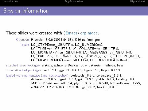
Session information
These slides were created with (Emacs) org mode.
R version R version 3.0.0 (2013-04-03), i686-pc-linux-gnu
locale LC_CTYPE=en_GB.UTF-8, LC_NUMERIC=C,LC_TIME=en_GB.UTF-8, LC_COLLATE=en_GB.UTF-8,LC_MONETARY=en_GB.UTF-8, LC_MESSAGES=en_GB.UTF-8,LC_PAPER=C, LC_NAME=C, LC_ADDRESS=C, LC_TELEPHONE=C,LC_MEASUREMENT=en_GB.UTF-8, LC_IDENTIFICATION=C
attached base packages stats, graphics, grDevices, utils, datasets, methods, base
other attached packages ascii_2.1, ggplot2_0.9.3.1, bigvis_0.1, Rcpp_0.10.3
loaded via a namespace (and not attached) codetools_0.2-8, colorspace_1.2-2,dichromat_2.0-0, digest_0.6.3, grid_3.0.0, gtable_0.1.2, labeling_0.1,MASS_7.3-26, munsell_0.4, plyr_1.8, proto_0.3-10, RColorBrewer_1.0-5,reshape2_1.2.2, scales_0.2.3, stringr_0.6.2, tools_3.0.0

Introduction Bigvis overview Bigvis demo
Birmingham R User Meeting (BRUM)
www.birminghamR.org
Alastair Sanderson Ph.D. - www.AlastairSanderson.com