summer 2012 7

Report Visualisation of User Defined Finite Elements with ABAQUS/Viewer

Abstract Commercial finite element (FE) software packages provide inter-faces for user defined subrouti-nes, e.g. to define a user defined material behaviour or special pur- pose finite elements, respec-tively. Regarding the latter, the major drawback of user defined elements in Abaqus is that they can not be visualised with the standard post-processing tool Abaqus/Viewer. The reason for this is that the element topolo-gy is hidden inside the element subroutine.The software tool presented within this contribution closes this gap in order to utilise the powerful Abaqus postprocessing potentials. Because only elements from the Abaqus element library can be visualised with Abaqus/Viewer, the user elements in the output data bases resulting from FE calculations are replaced with properly chosen elements from the Abaqus standard ele-ment library. Furthermore, user element related data are taken from the binary results files and transferred consistently to these standard elements. This is done by means of the Abaqus Python scripting interface and requires the provision of additional user defined information concerning the element topology.The capabilities of this software tool are demonstrated with user defined elements developed for non-local damage mechanics, gradient elasticity, cohesive zone models and ferroelectricity.

1. IntroductionFinite element (FE) solution schemes require in general a

Visualisation of User Defined Finite Elements with ABAQUS/ViewerS. Roth, G. Hütter, U. Mühlich, B. Nassauer, L. Zybell, M. KunaInstitute of Mechanics and Fluid Dynamics, TU Bergakademie Freiberg

rather complex overhead inclu-ding the pre-processing, proper data organisation etc. In addi-tion, sophisticated solvers, con-tact algorithms or other tools are involved. Furthermore, the amount of manpower and time needed for the maintenance of such complex software soluti-ons should not be underesti-mated.The user element interface pro-vided by the commercial FE pro-gram Abaqus enables researches working in different fields of continuum mechanics, to focus exclusively on their specific pro-blems without being forced to take care of the topics mentioned above. Unfortunately, Abaqus can only visualise built-in ele-ments with the corresponding post-processing tool, Abaqus/Viewer. However, Abaqus pro- vides tools to extract informa-tion from output database files. The latter contain all requested data of the FE analysis including model information and results. The particular structure of these files relies on the Abaqus data convention which is documen-ted in the corresponding manuals [1]. Therefore, all the necessary information can be extracted, en- riched and re-structured in order to use the outcome of this pro-cess for the Abaqus/Viewer. The use of another post-processing software would be possible too, but there are certain objections concerning this idea. First of all, it is rather unlikely that alter-native visualisation tools provi-de all the specific facilities sup-ported by the Abaqus/Viewer. The simultaneous use of various tools according to their parti-

cular advantages is not seen as a suitable alternative ei- ther. Second, independent of the particular choice, data conversi-on has to be performed always. This means that the use of other post-processing tools than the Abaqus/Viewer would not pro-vide any benefit regarding the development cycle of the soft-ware necessary to achieve the desired objective.A particular strategy for the visualisation of user elements is sketched already in the Abaqus manuals. However, this strategy has several serious drawbacks. Here, a solution is proposed that resolves these problems.The paper is organised as follows. First, the Abaqus data structu-re is examined in order to de- rive the minimum requirements for a suitable visualisation stra- tegy. Subsequently, different pos-sibilities to accomplish the task are outlined and the particular advantages and disadvantages are discussed, focusing espe-cially on the solution proposed here. Afterwards, the latter is described in more detail and its capabilities are demonstrated by means of several illustrative examples.

2. Visualisation strategiesPlotting of user elements is not supported in Abaqus/CAE [1]. The Abaqus/Viewer only supports the visualisati-on of built-in elements of the Abaqus element library, which are hereinafter referred to as standard elements. There is no interface to specify user de- fined elements in the viewer. This leads to the questions what

summer 20128

Visualisation of User Defined Finite Elements with ABAQUS/Viewer Report

type of interface would be neces-sary to overcome this and which element data should be transfer-red? For visualisation purpose, the viewer requires the topological data of the finite elements. In this context, element topology covers the number of nodes and the definition of vertices, edges and faces which specifies the nodes mutual positions. Furthermore, in order to plot integration point data like stresses or state variables, the number of the integration points as well as their position inside the element are of interest. Finally, the shape functions de- fine an inter- and extrapolation algorithm to determine the inte-gration point values out of nodal data and vice versa, respectively. Of course, all this information is enclosed in the user element subroutine. But outside, only the number of nodes, the nodal degree of freedom (DOF) and the amount of memory require-ments for internal state variables are known. This suffices for the FE solution procedure but not for visualisation. Here, it should be emphasised, that these pro-blems are not only limited to the Abaqus framework. Pre- and post-processing of ANSYS user elements, for instance, is bound to the specification of a so-called keyshape value determining the elements topology [2].However, in order to use Abaqus/Viewer to visualise user elements in spite of all, additional effort is unavoidable. Thus, alternative standard elements, in the follo-wing called dummy elements, are chosen from the Abaqus element library and displayed in place of the user elements. Therefore, the topology of the dummy elements and the user elements should be as similar as possible. This concerns the element shape (e.g. hex, wedge or tet in 3D), the number of nodes, the order of the shape functions and the numeri-

cal integration (number and posi-tion of integration points). It is part of the developers job to find a balance between the restrictions concerning functionality of the user element and its visualisation ability with the help of an appli-cable dummy element. Mostly, a compromise is found since the element library provides a large variety of standard elements.The next step towards a successful visualisation is the extraction of the nodal and integration point result data from a data base. Therefore, the internal data struc-ture of the output database file (odb) is considered, wherein field output is assigned according to a so-called field location which specifies the position for which field data are available (e.g. node, integration point) [1]. Regarding user elements, the information about the field location and inte-gration points is hidden inside the element subroutine and thus the assignment of user element related result data fails. For this reason, user element output is written to either results file (fil) or data file (dat) while nodal field variables can be written to odb, fil or dat. A further important aspect concerns the interpretation of the element output. The array of solution dependent variables (SDV) is composed by the user element subroutine and can be split into several integration point related SDV arrays. A decomposi-tion of them into field quantities requires additional information about their name, description and tensorial rank. The latter is necessary to allow Abaqus to pro-vide the tensor invariants.In summary, a visualisation inter-face has to manage1. the input of additional element data concerning element toplogy, the desired dummy element and SDV arrangement,2. the generation of the dummy element mesh,

3. the transfer of nodal data and SDV to the odb, and4. the two-step decomposition of the SDV array with respect to the number of integration points and the embedded field quantities.There are a couple of approa-ches within the Abaqus frame-work discussed in the following. Afterwards, the favoured one is described in more detail.

2.1. State of the artIn order to visualise the shape of user elements, the Abaqus Analysis User’s Manual [1] propo-ses an overlaid mesh of standard elements generated during the pre-processing. In combination with an almost vanishing materi-al stiffness associated, the overlaid dummy element mesh allows the visualisation of the deformation state [1]. The spurious influence of the dummy element mesh on the numerical result is elimi-nated if an additional dummy user material is defined just crea-ting zero stiffness matrices [3]. Furthermore, the definition of the dummy elements with the help of the existing nodes of the user element mesh allows for visualisation of all nodal field quantities, e.g. displacements, nodal temperatures and reaction forces. Regarding the computa-tional cost, the additional effort is limited then to the evaluation of the dummy material subroutines. The size of the system matrices of the finite element models is not affected as neither the number of nodes nor the nodal DOF chan-ges. The latter requires a compa-tibility between the nodal DOF of the user element and the dummy element which limits the choice of possible dummy elements. Concerning the transfer of ele-ment output, it is recommended to use the subroutine UVARM, which is called at the end of every increment at every integra-tion point of the dummy element

summer 2012 9

Report Visualisation of User Defined Finite Elements with ABAQUS/Viewer

mesh to generate element output. The exchange of data between the UVARM subroutine and the cor-responding user element subrou-tine is usually managed via com-mon blocks, i.e. shared memory, or modules. Unfortunately, the use of common blocks is expli-citly precluded for multiprocessing applications [1] which gives rise to the major drawback of the data transfer via UVARM. The renouncement of efficient com-putational performance, i.e. par-allel computing, for the benefit of visualisation seems to be a poor compromise especially regarding the simulation of large models. Furthermore, in order to inter-pret the element output, sub-sequent post-processing remains indispensable since the UVARM just passes the still unstructured SDV array of the respective inte-gration points. Last, the increase of computational time due to the dummy element operations is considerable, depending on the number of user and dummy ele-ments, respectively.Thus, it can be stated that the strategy presented does not meet all the requirements of a visua-lisation interface mentioned above. In particular, the limiting interaction with the numerical computation is hardly acceptable. Instead, an independent visuali-sation module, applicable to arbi-trary user elements should be envisaged.

2.2. Postprocessing visualisation strategyThe visualisation strategy pro-posed here, called hereafter Abaquser, is a post-processing approach. In contrast to the strate-gy described before, the FE calcula-tions are not affected and there are no spurious enlargement of com-putational time or other restric-tions to be met. Abaquser bases on the Abaqus Python scripting interface which is used to add

model and result data to the odb after extraction from fil. Moreover, decomposition and interpretation of the SDV array is performed, too. Before presenting this pure post-processing script package in more detail and demonstrating its capabilities, it should be mentio-ned that there is a third applicable alternative of visualising user ele-ments. It comprises the combi-nation of both strategies, i.e. the pre-processing generation of an overlaid dummy element mesh with zero-stiffness user material combined with a post-processing transfer of element data from fil to odb. Compared to pure post-pro-cessing, the latter strategy yields less post-processing costs since there is no need to transfer nodal data. In return, the modelling of the overlaid mesh and the eva-luation of the dummy elements material subroutine result in com-paratively higher pre-processing and computational costs.

3. AbaquserAbaquser, a collection of shell and Python scripts manages all operations required to get an odb, which can be visualised with Abaqus/Viewer, for a given FE model containing user elements. It comprises four scopes explai-ned in the following. A schematic diagram of the working sequence of Abaquser is depicted in Figure 1.

3.1. Controlling the FE calcu-lation and visualisation post-processingAll relevant processes related to the visualisation are controlled by a shell script, abaquser.sh. Since the objective includes an input file check with respect to all indispensable conventions, this involves the submission of the FE job, too. Its command syntax resembles the syntax of the Abaqus command abaqus [1] supple-mented by an option to spe-cify the information file contai-ning all additional data required. After the FE calculation has been completed successfully, visualisa-tion post-processing is initiated immediately.

3.2. Extraction of model and result data from data baseModel and result data can be extracted out of different data sources. Since the efficiency of the visualisation process and its accuracy is quite sensitive to this choice, here, the potential sour-ces are discussed briefly. Thereby,it is appropriate to distinguish between model and result data. Model data related to user ele-ments are available in the input file, dat or fil. User elements result data can be written to dat or fil. Although implemented easily and used severalfold, the use of the ASCII format dat (see

Figure 1: Visualisation process of Abaquser.Figure 1:

summer 201210

Visualisation of User Defined Finite Elements with ABAQUS/Viewer Report

e.g. [4]) is not a good choice as data base, because writing to the dat rai-ses computational time significant-ly. Furthermore, in comparison to the binary fil, there are major sto-rage requirements and less reading speed. Due to the fixed number format, the accuracy is limited. For these reasons, the binary fil, which, incidentally, can be written, too, in ASCII format, is chosen to be the preferred data source. It should be mentioned, that to the author’s knowledge, visualisation of result data taken from fil by means of Abaqus/Viewer is not published so far. To access the results file information, Abaqus provides a well described Fortran interface [1] which is, however, not used here.Unfortunately, the model data in the fil are not organised in the assembly-instance structure which the Python interface expects to update the odb. Nevertheless, it is possible to re-build the desi-red structure with the help of the respective node and element labels, which contain the assembly as well as the instance labels. This leads to the requirement that each of the nodes and elements defined in the pre-processing has to belong to at least one set whose label is evalu-ated later on. Otherwise, this entity can not be assigned to an instance and its visualisation fails.

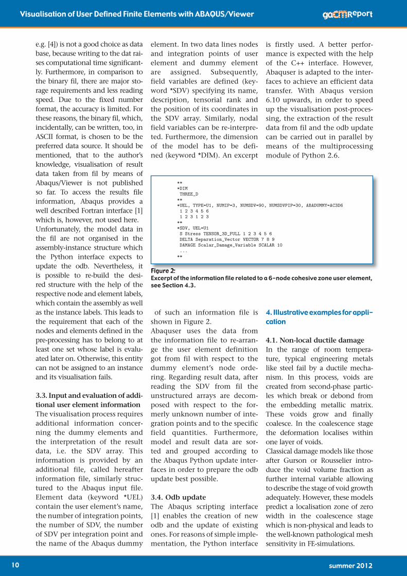
3.3. Input and evaluation of addi-tional user element informationThe visualisation process requires additional information concer-ning the dummy elements and the interpretation of the result data, i.e. the SDV array. This information is provided by an additional file, called hereafter information file, similarly struc-tured to the Abaqus input file. Element data (keyword *UEL) contain the user element’s name, the number of integration points, the number of SDV, the number of SDV per integration point and the name of the Abaqus dummy

element. In two data lines nodes and integration points of user element and dummy element are assigned. Subsequently, field variables are defined (key-word *SDV) specifying its name, description, tensorial rank and the position of its coordinates in the SDV array. Similarly, nodal field variables can be re-interpre-ted. Furthermore, the dimension of the model has to be defi-ned (keyword *DIM). An excerpt

of such an information file is shown in Figure 2.Abaquser uses the data from the information file to re-arran-ge the user element definition got from fil with respect to the dummy element’s node orde-ring. Regarding result data, after reading the SDV from fil the unstructured arrays are decom-posed with respect to the for-merly unknown number of inte-gration points and to the specific field quantities. Furthermore, model and result data are sor-ted and grouped according to the Abaqus Python update inter-faces in order to prepare the odb update best possible.

3.4. Odb updateThe Abaqus scripting interface [1] enables the creation of new odb and the update of existing ones. For reasons of simple imple-mentation, the Python interface

is firstly used. A better perfor-mance is expected with the help of the C++ interface. However, Abaquser is adapted to the inter-faces to achieve an efficient data transfer. With Abaqus version 6.10 upwards, in order to speed up the visualisation post-proces-sing, the extraction of the result data from fil and the odb update can be carried out in parallel by means of the multiprocessing module of Python 2.6.

4. Illustrative examples for appli-cation

4.1. Non-local ductile damageIn the range of room tempera-ture, typical engineering metals like steel fail by a ductile mecha-nism. In this process, voids are created from second-phase partic-les which break or debond from the embedding metallic matrix. These voids grow and finally coalesce. In the coalescence stage the deformation localises within one layer of voids.Classical damage models like those after Gurson or Rousselier intro-duce the void volume fraction as further internal variable allowing to describe the stage of void growth adequately. However, these models predict a localisation zone of zero width in the coalescence stage which is non-physical and leads to the well-known pathological mesh sensitivity in FE-simulations.

Figure 2:Excerpt of the information file related to a 6-node cohesive zone user element, see Section 4.3.

Figure 2:

***DIMTHREE_D

***UEL, TYPE=U1, NUMIP=3, NUMSDV=90, NUMSDVPIP=30, ABADUMMY=AC3D61 2 3 4 5 61 2 3 1 2 3

***SDV, UEL=U1S Stress TENSOR_3D_FULL 1 2 3 4 5 6DELTA Separation_Vector VECTOR 7 8 9DAMAGE Scalar_Damage_Variable SCALAR 10...

**

Figure 2: Excerpt of the information file related to a 6-node cohesive zone user element, see Section 4.3.

Abaquser uses the data from the information file to re-arrange the user element definition got from filwith respectto the dummy element’s node ordering. Regarding result data, after reading the SDV from fil the unstructured arraysare decomposed with respect to the formerly unknown number of integration points and to the specific field quantities.Furthermore, model and result data are sorted and grouped according to the Abaqus Python update interfaces in orderto prepare the odb update best possible.

3.4. Odb update

The Abaqus scripting interface [1] enables the creation of new odb and the update of existing ones. For reasonsof simple implementation, the Python interface is firstly used. A better performance is expected with the help of theC++ interface. However, Abaquser is adapted to the interfaces to achieve an efficient data transfer. With Abaqusversion 6.10 upwards, in order to speed up the visualisation post-processing, the extraction of the result data from fil

and the odb update can be carried out in parallel by means of the multiprocessing module of Python 2.6.

4. Illustrative examples for application

4.1. Non-local ductile damage

In the range of room temperature, typical engineering metals like steel fail by a ductile mechanism. In thisprocess, voids are created from second-phase particles which break or debond from the embedding metallic matrix.These voids grow and finally coalesce. In the coalescence stage the deformation localises within one layer of voids.

Classical damage models like those after Gurson or Rousselier introduce the void volume fraction as furtherinternal variable allowing to describe the stage of void growth adequately. However, these models predict a localisationzone of zero width in the coalescence stage which is non-physical and leads to the well-known pathological meshsensitivity in FE-simulations.

For this reason, a non-local modification of the Gurson-model was developed [5]. In a so-called implicit gradient-enriched formulation a further partial differential equation is incorporated introducing an intrinsic length scale as afurther material parameter. This intrinsic length can be correlated to the mean spacing of the voids and allows tocontrol the width of the localisation zone of void coalescence in the simulations.

The weak form of the further partial differential equation has to be included in the FE-formulation as additional setof equations. Correspondingly, the non-local variable (the non-local volumetric plastic strain) enters as nodal variable.The additional non-local equations are implemented as a user defined element via the UEL interface.

Three-dimensional hexahedral as well as two-dimensional plain-strain and axisymmetric elements have been de-veloped in a large displacement formulation for static or dynamic applications. Quadratic shape functions are usedfor the geometry and the displacements and linear ones for the non-local volumetric plastic strain. Full or reducedintegration is available. The Abaqus built-in elements CPE8, CPE8R, C3D20 or C3D20R are used as dummy elementsfor the visualisation with Abaquser. Figure 3 shows the distribution of the void volume fraction in the late stage of thenecking in a tensile test simulated with the non-local Gurson implementation in Abaqus.

5

summer 2012 11

Report Visualisation of User Defined Finite Elements with ABAQUS/Viewer

For this reason, a non-local modi-fication of the Gurson-model was developed [5]. In a so-called implicit gradientenriched formu-lation a further partial differential equation is incorporated introdu-cing an intrinsic length scale as a further material parameter. This intrinsic length can be correlated to the mean spacing of the voids and allows to control the width of the localisation zone of void coalescence in the simulations. The weak form of the further par-tial differential equation has to be included in the FE-formulation as additional set of equations. Correspondingly, the non-local variable (the non-local volume-tric plastic strain) enters as nodal variable. The additional non-local equations are implemented as a user defined element via the UEL interface.

4.2. Quasi-brittle strain gradient damageModels aiming to describe qua-si-brittle failure must incorpo-rate the evolution of damage. Furthermore, they should account for deterministic size effects and the numerical results obtained by these models must not show any spurious mesh dependence. Based on the constitutive equations for strain gradient elasticity derived in [6] and [7] a continuum damage model has been developed. It rests on the idea to describe the damage evolution in porous elastic materi-als by means of the evolution of an effective porosity which can increase beyond an initial value f0, related to the undamaged porous material, up to a final porosity somewhere in between the initial value and one. The main ingre-dient of the damage model is a

Three-dimensional hexahedral as well as two-dimensional plain-strain and axisymmetric ele-ments have been developed in a large displacement formulation for static or dynamic applicati-ons. Quadratic shape functions are used for the geometry and the displacements and linear ones for the non-local volumetric plastic strain. Full or reduced integration is available. The Abaqus built-in elements CPE8, CPE8R, C3D20 or C3D20R are used as dummy ele-ments for the visualisation with Abaquser. Figure 3 shows the distribution of the void volume fraction in the late stage of the necking in a tensile test simula-ted with the non-local Gurson implementation in Abaqus.

Figure 3: Distribution of the void volume fraction after necking in a tensile test.

Figure 4: Final damage state (porosity f ) obtained with regular finite element meshes using different element edge lengths along the path from the upper left corner to the lower right corner of the square (lhs). The contour plot of the damage variable (rhs) corresponds to the simulation performed with the finest mesh = 1/64. The ratio between the length of the square and the internal length R is 0.25, see e.g. [6]. An initial porosity f0 = 0.1 was used for all simulations and the final porosity fF was set to fF = 0.95.

Figure 4:

summer 201212

Visualisation of User Defined Finite Elements with ABAQUS/Viewer Report

damage surface which depends on the macroscopic strains, its spatial gradients and the effective porosity f.The appearance of strain gradients or second gradients of the dis-placements, respectively, requires the use of either C(1)-continuous finite elements or a suitable mixed finite element formulation. Here, the latter was preferred using additional Lagrange multipliers. Nevertheless, neither one of these two options mentioned above forms part of the current stan-dard element library of Abaqus. Therefore, a user defined solution is unavoidable, anyway. The damage model has been implemented into the FE program Abaqus extending the user element already described in [8]. The nine noded element contains two displacements at all nodes, four additional strains at the corner nodes and four Lagrange multipliers at the middle node. Furthermore, the standard CPE8 element is used as dummy element.The convergence behaviour of the damage model has been studied by means of the following pro-blem. A unit square is exposed to quadratic boundary displacements

0.020.040.060.080.100.120.140.160.190.210.230.250.27

Figure 3: Distribution of the void volume fraction after necking in a tensile test.

4.2. Quasi-brittle strain gradient damage

Models aiming to describe quasi-brittle failure must incorporate the evolution of damage. Furthermore, theyshould account for deterministic size effects and the numerical results obtained by these models must not show anyspurious mesh dependence. Based on the constitutive equations for strain gradient elasticity derived in [6] and [7] acontinuum damage model has been developed. It rests on the idea to describe the damage evolution in porous elasticmaterials by means of the evolution of an effective porosity which can increase beyond an initial value f0, relatedto the undamaged porous material, up to a final porosity somewhere in between the initial value and one. The mainingredient of the damage model is a damage surface which depends on the macroscopic strains, its spatial gradientsand the effective porosity f .

The appearance of strain gradients or second gradients of the displacements, respectively, requires the use ofeither C(1)-continuous finite elements or a suitable mixed finite element formulation. Here, the latter was preferredusing additional Lagrange multipliers. Nevertheless, neither one of these two options mentioned above forms partof the current standard element library of Abaqus. Therefore, a user defined solution is unavoidable, anyway. Thedamage model has been implemented into the FE program Abaqus extending the user element already described in[8]. The nine noded element contains two displacements at all nodes, four additional strains at the corner nodes andfour Lagrange multipliers at the middle node. Furthermore, the standard CPE8 element is used as dummy element.

u1 = 0.05( 12 x2

1 + x22) and u2 = 0.05(−x2

1 +12 x2

2) referring to a

with diff / /64. Parts of the resultsare shown in Figure 4.

−√2

√20

0.50

0.95

1.00

f ∆ = 1/8∆ = 1/16∆ = 1/32∆ = 1/64

Figure 4: Final damage state (porosity f ) obtained with regular finite element meshes using different element edge lengths ∆ along the path fromthe upper left corner to the lower right corner of the square (lhs). The contour plot of the damage variable (rhs) corresponds to the simulationperformed with the finest mesh ∆ = 1/64. The ratio between the length of the square and the internal length R is 0.25, see e.g. [6]. An initialporosity f0 = 0.1 was used for all simulations and the final porosity fF was set to fF = 0.95.

6

and

0.020.040.060.080.100.120.140.160.190.210.230.250.27

Figure 3: Distribution of the void volume fraction after necking in a tensile test.

4.2. Quasi-brittle strain gradient damage

Models aiming to describe quasi-brittle failure must incorporate the evolution of damage. Furthermore, theyshould account for deterministic size effects and the numerical results obtained by these models must not show anyspurious mesh dependence. Based on the constitutive equations for strain gradient elasticity derived in [6] and [7] acontinuum damage model has been developed. It rests on the idea to describe the damage evolution in porous elasticmaterials by means of the evolution of an effective porosity which can increase beyond an initial value f0, relatedto the undamaged porous material, up to a final porosity somewhere in between the initial value and one. The mainingredient of the damage model is a damage surface which depends on the macroscopic strains, its spatial gradientsand the effective porosity f .

The appearance of strain gradients or second gradients of the displacements, respectively, requires the use ofeither C(1)-continuous finite elements or a suitable mixed finite element formulation. Here, the latter was preferredusing additional Lagrange multipliers. Nevertheless, neither one of these two options mentioned above forms partof the current standard element library of Abaqus. Therefore, a user defined solution is unavoidable, anyway. Thedamage model has been implemented into the FE program Abaqus extending the user element already described in[8]. The nine noded element contains two displacements at all nodes, four additional strains at the corner nodes andfour Lagrange multipliers at the middle node. Furthermore, the standard CPE8 element is used as dummy element.

u1 = 0.05( 12 x2

1 + x22) and u2 = 0.05(−x2

1 +12 x2

2) referring to a

with diff / /64. Parts of the resultsare shown in Figure 4.

−√2

√20

0.50

0.95

1.00

f ∆ = 1/8∆ = 1/16∆ = 1/32∆ = 1/64

Figure 4: Final damage state (porosity f ) obtained with regular finite element meshes using different element edge lengths ∆ along the path fromthe upper left corner to the lower right corner of the square (lhs). The contour plot of the damage variable (rhs) corresponds to the simulationperformed with the finest mesh ∆ = 1/64. The ratio between the length of the square and the internal length R is 0.25, see e.g. [6]. An initialporosity f0 = 0.1 was used for all simulations and the final porosity fF was set to fF = 0.95.

6

referring to aCartesian coordinate system with the origin in the upper left cor-ner of the square. The simulati-ons were performed with different

regular meshes varying the edge size of the finite elements from 1/8 down to 1/64. Parts of the results are shown in Figure 4. Because the visualisation tool enables the user to take advan-tage of all features provided by Abaqus/Viewer, like contour plots, plots of variables along a path, etc., it is not just useful to-gether with the final user element solution but it is also extreme-ly helpful during the process of implementation and testing.

4.3. Fatigue crack growth of thermally sprayed coatingsThe simulation of thermo-mecha-nical fatigue of thermally spray-ed coatings is performed with the help of cohesive zone user elements (CZE) [9]. The coating consists of deformed, flattened particles separated by thin oxide layers, where damage accumula-tion is supposed to be situated. A representative volume element (RVE of the coating structure) is depicted in Figure 5. The partic-le distribution is obtained by Voronoi-tessellation taking into account the mean diameter of the initially globular spraying partic-les. Both, substrate and particles are assumed to be linear elastic.The traction-separation relation at the interfaces between the coa-ting particles and between coa-ting and substrate are described with a cyclic cohesive zone model

[10]. Misfits of elastic modulus and thermal expansion coeffcient cause thermo-mechanical fatigue when the structure is subjected to cyclic thermal loading. Figure 6 shows the distribution of damage at the honeycomb-like CZE mesh after various load cycles.The implemented CZE provide both linear as well as quadra-tic shape functions, which are not supported in Abaqus [1]. Moreover, in contrast to Abaqus standard cohesive elements true stress and strain tensors are avai-lable. In 3D stress/displacement analyses with 12 node quadratic wedge-shaped CZE linear acou-stic AC3D6 elements with hig-her order integration are used as dummy elements. This choice succeeds only using the pure post-processing strategy. Otherwise, the overlay mesh of acoustic ele-ments increases the nodal DOF which leads to an unnecessary inflation of the system matrices

Figure 6: Damage distribution after 4 and 9 thermal load cycles, cut view through RVE.Figure 6:

Figure 5: RVE of a thermally sprayed coating structure.

Figure 5:

summer 2012 13

Report Visualisation of User Defined Finite Elements with ABAQUS/Viewer

and computational cost, respec-tively. The visualisation is mainly focused on the damage distributi-on and allows the quantification of fatigue crack growth within the cohesive zone and decohesi-on or delamination, respectively.

4.4. Micromechanical material model for ferroelectric ceramicsMaterial models comprising elec-tro-mechanical coupling can not be implemented by means of the Abaqus UMAT interface. Instead, the implementation of a user defi-ned element is necessary which is presented here for a micromecha-nical ferroelectric material model. Ferroelectric ceramics are charac-terised by a nonlinear material behaviour with electro-mechanical coupling. The micromechanical material model employed here is mainly based on works of Huber et al [11] and Pathak and McMeeking [12], see [13]. The idea of the model is to consider the ferroelectric poly-crystal as single crystals with speci-fic lattice orientations. Each of the crystals consists of several domains with different spontaneous polari-sation directions. Assuming tetrago-nal material, eight domain variants are possible in three-dimensional space. The volume fractions of these domains can change if an electric field or mechanical stress is applied. This change is called domain switching and is determi-ned in the model by an energy-

based switching criterion. Due to switching, the average polarisation vector, the remanent strain and the average mechanical, electrical and piezoelectrical material proper-ties of the crystal change, resul-ting in a nonlinear macroscopic response. The material model is implemented in Abaqus by means of a three-dimensional user element including a material subroutine. The latter calculates the material tensors resulting from the volume fractions of the different domains and the orientation of the crystal. The change of the volume fractions due to domain switching is calcu-lated, too. The piezoelectric C3D8E standard Abaqus elements are used as dummy elements. The polarisa-tion is visualised as an additional field variable.The ferroelectric user element is employed to simulate a stack actua-tor. Figure 7 shows the polarisation and the stress field around the tip of an electrode. The discontinuities in the stress field result from different material properties of the individual grains having different lattice ori-entations. The borders between the grains are marked by red lines.

5. ConclusionAbaquser provides visualisation of user defined elements by means of Abaqus/Viewer in a general appli-cable way. Apart of some conven-tions, there are no restrictions to either the user element subrouti-

Figure 7:Polarisation (lhs) and stress field (max. principal, rhs) around the tip of an electrode.Figure 7:

nes or the FE calculations. Instead, all information Abaquser requires is passed in by a small informa-tion file which reduces the user’s job to a minimum. Abaquser uses a post-processing approach based on the extraction of model and result data from fil. It should be emphasised that the existence of fil which is more or less a relict of former Abaqus versions, is the necessary precondition to perform this kind of visualisation.

AcknowledgementThis work was performed within the Cluster of Excellence ”Structure Design of Novel High-Performance Materials via Atomic Design and Defect Engineering (ADDE)” that is financially supported by the European Union (European regio-nal development fund) and by the Ministry of Science and Art of Saxony (SMWK).

Corresponding author/E-Mail address:

Stephan.Roth@imfd.tu-freiberg.de

URL: http://tu-freiberg.de/fakult4/imfd/

summer 201214

Visualisation of User Defined Finite Elements with ABAQUS/Viewer Report

References[1] Dassault Systèmes. Abaqus 6.10 Online

Documentation, 2010.

[2] ANSYS, Inc. ANSYS Release 13.0, ANSYS

Mechanical APDL Programmer’s Manual, 2010.

[3] L.P. Mikkelsen. Implementing a gradient

dependent plasticity model in abaqus. In 2007

Abaqus User’s Conference, SIMULIA, Paris,

France, page 482–492, 2007.

[4] L. Zybell, U. Mühlich, and M. Kuna.

Implementierung von gradientenelastizität über

die schnittstelle uel. In 20. Deutschsprachige

Abaqus-Benutzerkonferenz, Bad Homburg,

Germany, 2008.

[5] T. Linse, G. Hütter, and M. Kuna. Simulation of

crack propagation using a gradient-enriched duc-

tile damage model based on dilatational strain.

submitted to Engineering Fracture Mechanics.

[6] L. Zybell, U. Mühlich, and M. Kuna.

Constitutive equations for porous plane-strain

gradient elasticity obtained by homogenization.

Archive of Applied Mechanics, 79(4):359–375,

2008.

[7] U. Mühlich, L. Zybell, and M. Kuna.

Micromechanical modelling of size effects in

failure of porous elastic solids using first order

plane strain gradient elasticity. Computational

Materials Science, 46(3):647–653, 2009.

[8] L. Zybell. Implementation of a user-ele-

ment considering strain gradient effects into

the fe-program abaqus. Master’s thesis, TU

BergakademieFreiberg, 2007.

[9] S. Roth and M. Kuna. Numerical study on

interfacial damage of sprayed coatings due to

thermo-mechanical fatigue. In E. Onate, D.R.J.

Owen, D. Peric, and B. Suarez, editors, XI

International Conference on Computational

Plasticity. Fundamentals and Applications.

COMPLAS XI., Barcelona, Spain, 2011.

[10] S. Roth and M. Kuna. Modelling of inter-

facial damage and delamination of sprayed

coatings with cohesive elements. In PAMM

Proceedings in Applied Mathematics and

Mechanics, 2011.

[11] J.E. Huber, N.A. Fleck, C.M. Landis,

and R.M. McMeeking. A constitutive model

for ferroelectric polycrystals. Journal of the

Mechanics and Physics of Solids, 47(8):1663–

1697, 1999.

[12] A. Pathak and R.M. McMeeking. Three-

dimensional finite element simulations of

ferroelectric polycrystals under electrical and

mechanical loading. Journal of the Mechanics

and Physics of Solids, 56(2):663–683, 2008.

[13] Q. Li, M. Enderlein, and Kuna M.

Micromechanical simulation of ferroelectric

domain switching at cracks. In M. Kuna and

A. Ricoeur, editors, IUTAM Symposium on

Multiscale Modelling of Fatigue, Damage

and Fracture in Smart Materials, IUTAM

Bookseries, volume 24, pages 101–110.

Springer Science+Business Media, 2011.