1

Visual DSD

User manual v0.14 beta: Matthew R. Lakin, Rasmus Petersen & Andrew Phillips

Introduction Visual DSD is an implementation of a programming language for composable DNA circuits based on

that described in (Phillips & Cardelli, 2009). The language includes basic elements of sequence

domains, toeholds and branch migration, and assumes that strands do not possess any secondary

structure. The Visual DSD tool compiles a collection of DNA molecules into a set of chemical

reactions. It also includes a stochastic simulator which computes a possible trajectory of the system

and graphs the populations of species over time and a deterministic simulator which forms and

solves an ODE representation of the dynamics of the system. Furthermore the reachable state space

of the system can be constructed as a continuous-time Markov chain.

This manual assumes that the user is familiar with the basics of DNA strand displacement and, in

particular, the terminology and notation from (Phillips & Cardelli, 2009). The reader is referred to

that paper for the technical details of the language semantics.

Installing Visual DSD Visual DSD is available in two forms: a Silverlight-based graphical application and a text-based

command-line tool.

In order to run the Silverlight version you must install the correct Silverlight plug-in for your

operating system and web browser from http://www.microsoft.com/silverlight.

Silverlight compatibility has been tested on Windows and Mac OS X under various browsers,

including Internet Explorer, Firefox, Safari and Chrome. With Silverlight installed, browse to

http://lepton.research.microsoft.com/webdna and the user interface should load

within a few seconds. In the top-right corner of the interface there is an “Install” button which you

can click to install a local copy of the Silverlight program – this should work both on Windows and on

Mac OS. We will describe the use of the Visual DSD Silverlight interface in the next section. Next to

the “Install” button is a “License” button which brings up a copy of the Visual DSD license

agreement. Once the software is installed, the “Install” button becomes an “Update” button which

can be used to check for, and install, any newer releases of the software.

Note that when a new version of the software is released online, you may need to “reset” your web

browser to delete the old version from the cache before your browser will load the new version.

There is also a command-line version of Visual DSD which is included in the source distribution as

pre-compiled binaries for Windows and Mac OS X 10.5. The command-line version can be compiled

using the F# or Objective Caml compilers and contains build scripts to automate this process under

Windows, Linux or Mac OS X. The command-line executable implements most of the functionality of

the Silverlight version. We describe the use of the Visual DSD command-line interface at the end of

this document.

2

Using Visual DSD under Silverlight The Visual DSD tool comes with a number of example systems implemented using DNA molecules.

These are accessible from the drop-down menu labeled “Examples” in the top-left corner of the

Silverlight user interface.

The Catalytic example is an implementation of the entropy-driven catalytic gate from (Zhang,

Turberfield, Yurke, & Winfree, 2007). The Lotka example is the Lotka-Volterra predator-prey

oscillator. The Mapk example models a mitogen-activated protein kinase (MAPK) signaling cascade

(Huang & Ferrel, 1996) and the Migrations example serves to demonstrate the branch migration rate

model (Zhang & Winfree, 2009). Most of the other examples are related to the implementation of

chemical kinetics using DNA. We will use the catalytic gate as a running example. Selecting this

populates the “Code” tab in the left-hand pane with the text of the example program – we can use

the “Zoom” slider to adjust the text size. We will return to the DNA tab below.

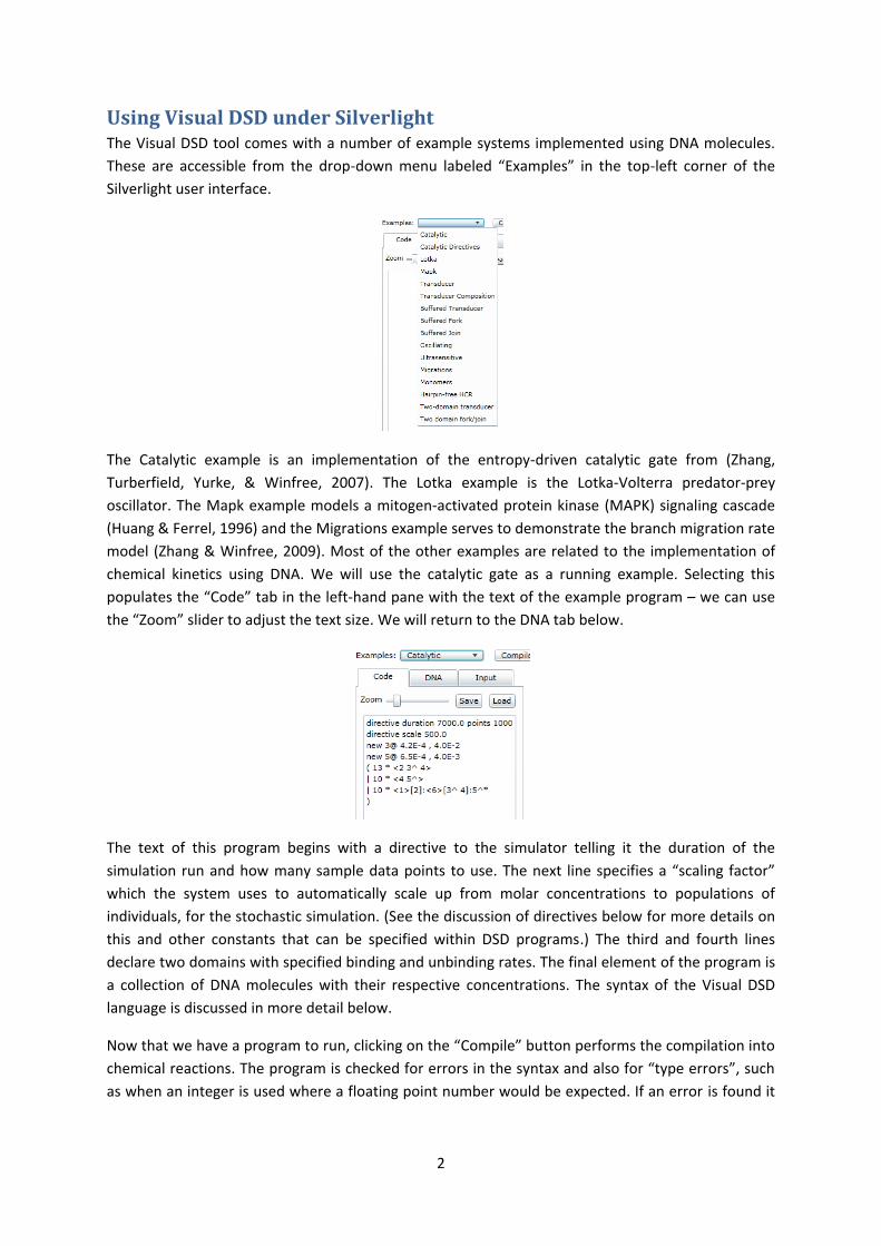
The text of this program begins with a directive to the simulator telling it the duration of the

simulation run and how many sample data points to use. The next line specifies a “scaling factor”

which the system uses to automatically scale up from molar concentrations to populations of

individuals, for the stochastic simulation. (See the discussion of directives below for more details on

this and other constants that can be specified within DSD programs.) The third and fourth lines

declare two domains with specified binding and unbinding rates. The final element of the program is

a collection of DNA molecules with their respective concentrations. The syntax of the Visual DSD

language is discussed in more detail below.

Now that we have a program to run, clicking on the “Compile” button performs the compilation into

chemical reactions. The program is checked for errors in the syntax and also for “type errors”, such

as when an integer is used where a floating point number would be expected. If an error is found it

3

is reported in a message box together with the location of the offending section of the program, like

the following example error message.

If the program is error-free then the compilation process proceeds as described in (Phillips &

Cardelli, 2009). This produces output in the “Initial” tab and in the six sub-tabs of the “Compilation”

tab on the right-hand side. This output persists until a modified program is compiled using the

“Compile” button.

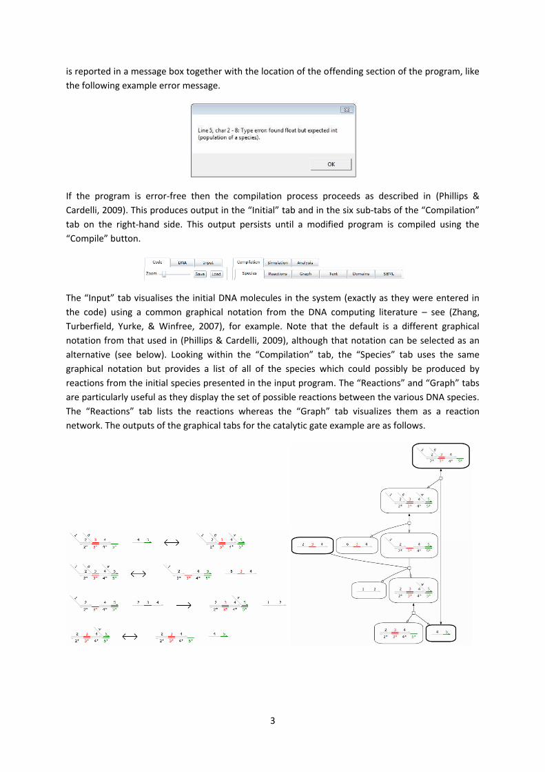
The “Input” tab visualises the initial DNA molecules in the system (exactly as they were entered in

the code) using a common graphical notation from the DNA computing literature – see (Zhang,

Turberfield, Yurke, & Winfree, 2007), for example. Note that the default is a different graphical

notation from that used in (Phillips & Cardelli, 2009), although that notation can be selected as an

alternative (see below). Looking within the “Compilation” tab, the “Species” tab uses the same

graphical notation but provides a list of all of the species which could possibly be produced by

reactions from the initial species presented in the input program. The “Reactions” and “Graph” tabs

are particularly useful as they display the set of possible reactions between the various DNA species.

The “Reactions” tab lists the reactions whereas the “Graph” tab visualizes them as a reaction

network. The outputs of the graphical tabs for the catalytic gate example are as follows.

4

Each labelled node in the “Graph” tab denotes a species. The initial species are represented with a

bold outline. Each unlabelled node represents a reaction, which may or may not be reversible, with

edges connected to reactant and product species. For irreversible reactions, edges with no arrows

denote reactants, while edges with hollow arrows denote products. For reversible reactions, hollow

and solid arrows are used to distinguish between the products of the forward and reverse reactions,

respectively.

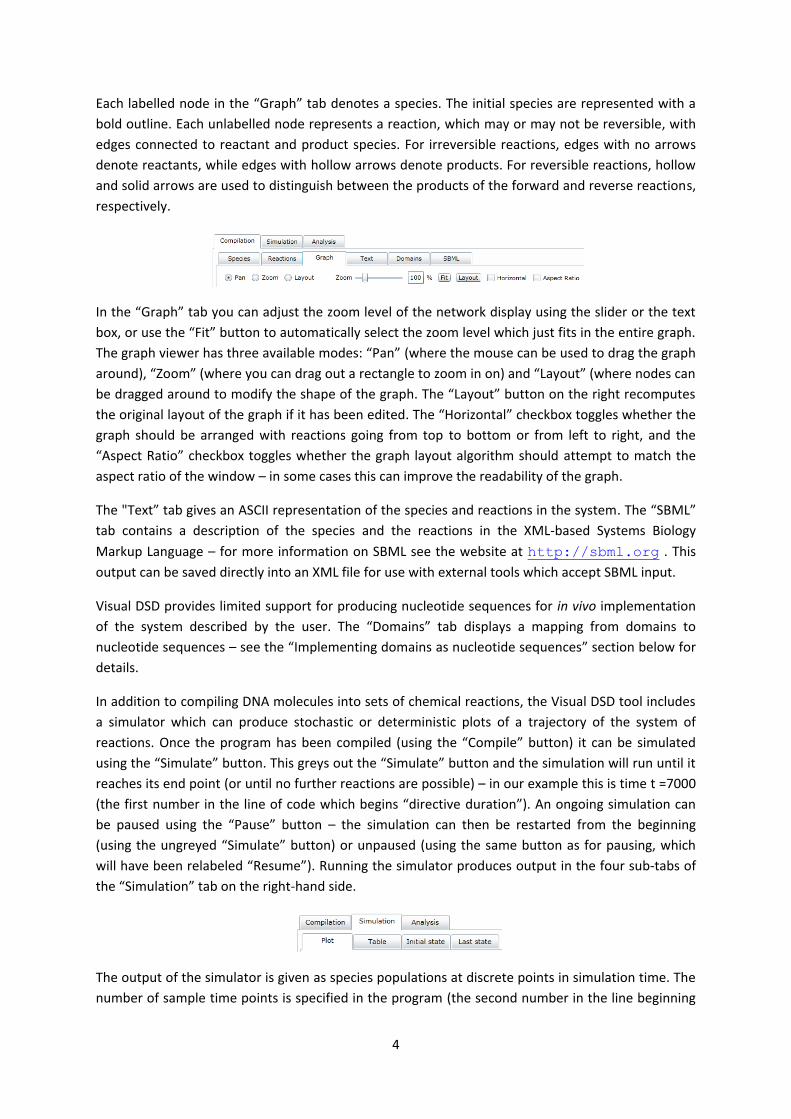
In the “Graph” tab you can adjust the zoom level of the network display using the slider or the text

box, or use the “Fit” button to automatically select the zoom level which just fits in the entire graph.

The graph viewer has three available modes: “Pan” (where the mouse can be used to drag the graph

around), “Zoom” (where you can drag out a rectangle to zoom in on) and “Layout” (where nodes can

be dragged around to modify the shape of the graph. The “Layout” button on the right recomputes

the original layout of the graph if it has been edited. The “Horizontal” checkbox toggles whether the

graph should be arranged with reactions going from top to bottom or from left to right, and the

“Aspect Ratio” checkbox toggles whether the graph layout algorithm should attempt to match the

aspect ratio of the window – in some cases this can improve the readability of the graph.

The "Text” tab gives an ASCII representation of the species and reactions in the system. The “SBML”

tab contains a description of the species and the reactions in the XML-based Systems Biology

Markup Language – for more information on SBML see the website at http://sbml.org . This

output can be saved directly into an XML file for use with external tools which accept SBML input.

Visual DSD provides limited support for producing nucleotide sequences for in vivo implementation

of the system described by the user. The “Domains” tab displays a mapping from domains to

nucleotide sequences – see the “Implementing domains as nucleotide sequences” section below for

details.

In addition to compiling DNA molecules into sets of chemical reactions, the Visual DSD tool includes

a simulator which can produce stochastic or deterministic plots of a trajectory of the system of

reactions. Once the program has been compiled (using the “Compile” button) it can be simulated

using the “Simulate” button. This greys out the “Simulate” button and the simulation will run until it

reaches its end point (or until no further reactions are possible) – in our example this is time t =7000

(the first number in the line of code which begins “directive duration”). An ongoing simulation can

be paused using the “Pause” button – the simulation can then be restarted from the beginning

(using the ungreyed “Simulate” button) or unpaused (using the same button as for pausing, which

will have been relabeled “Resume”). Running the simulator produces output in the four sub-tabs of

the “Simulation” tab on the right-hand side.

The output of the simulator is given as species populations at discrete points in simulation time. The

number of sample time points is specified in the program (the second number in the line beginning

5

“directive duration”). By default (as in the catalytic gate example) the simulator samples the

populations of all of the species in the system after every single reaction. It is possible

programmatically to restrict this to a subset of the species, as discussed in the next section.

The “Table” tab contains a tabular representation of the simulation data as species populations over

time. The data in this tab can be saved as a comma-separated (CSV) or tab-separated (TSV) file which

can then be imported into a spreadsheet such as Microsoft Excel. Alternatively, the data can be

copied and pasted directly into Excel as it stands.

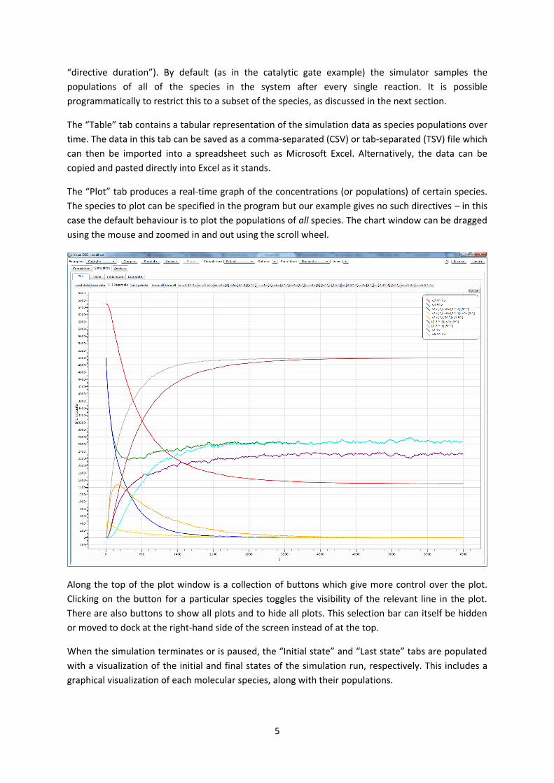
The “Plot” tab produces a real-time graph of the concentrations (or populations) of certain species.

The species to plot can be specified in the program but our example gives no such directives – in this

case the default behaviour is to plot the populations of all species. The chart window can be dragged

using the mouse and zoomed in and out using the scroll wheel.

Along the top of the plot window is a collection of buttons which give more control over the plot.

Clicking on the button for a particular species toggles the visibility of the relevant line in the plot.

There are also buttons to show all plots and to hide all plots. This selection bar can itself be hidden

or moved to dock at the right-hand side of the screen instead of at the top.

When the simulation terminates or is paused, the “Initial state” and “Last state” tabs are populated

with a visualization of the initial and final states of the simulation run, respectively. This includes a

graphical visualization of each molecular species, along with their populations.

6

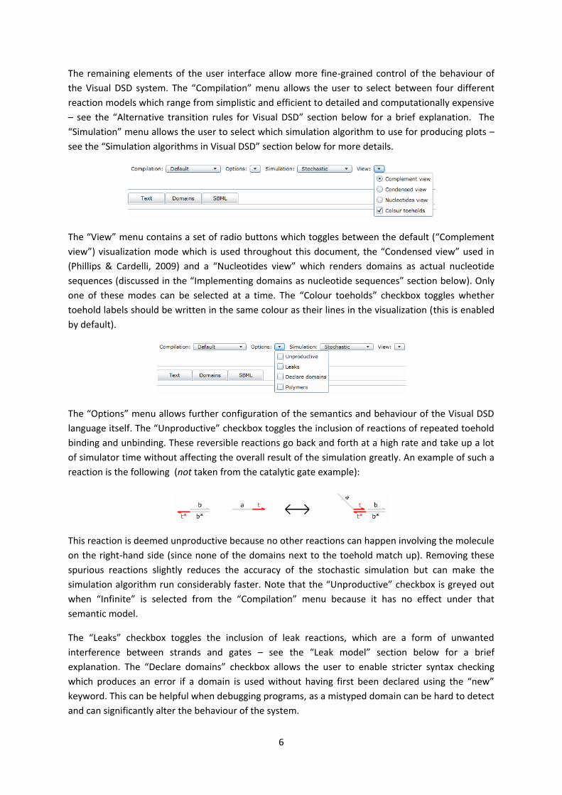
The remaining elements of the user interface allow more fine-grained control of the behaviour of

the Visual DSD system. The “Compilation” menu allows the user to select between four different

reaction models which range from simplistic and efficient to detailed and computationally expensive

– see the “Alternative transition rules for Visual DSD” section below for a brief explanation. The

“Simulation” menu allows the user to select which simulation algorithm to use for producing plots –

see the “Simulation algorithms in Visual DSD” section below for more details.

The “View” menu contains a set of radio buttons which toggles between the default (“Complement

view”) visualization mode which is used throughout this document, the “Condensed view” used in

(Phillips & Cardelli, 2009) and a “Nucleotides view” which renders domains as actual nucleotide

sequences (discussed in the “Implementing domains as nucleotide sequences” section below). Only

one of these modes can be selected at a time. The “Colour toeholds” checkbox toggles whether

toehold labels should be written in the same colour as their lines in the visualization (this is enabled

by default).

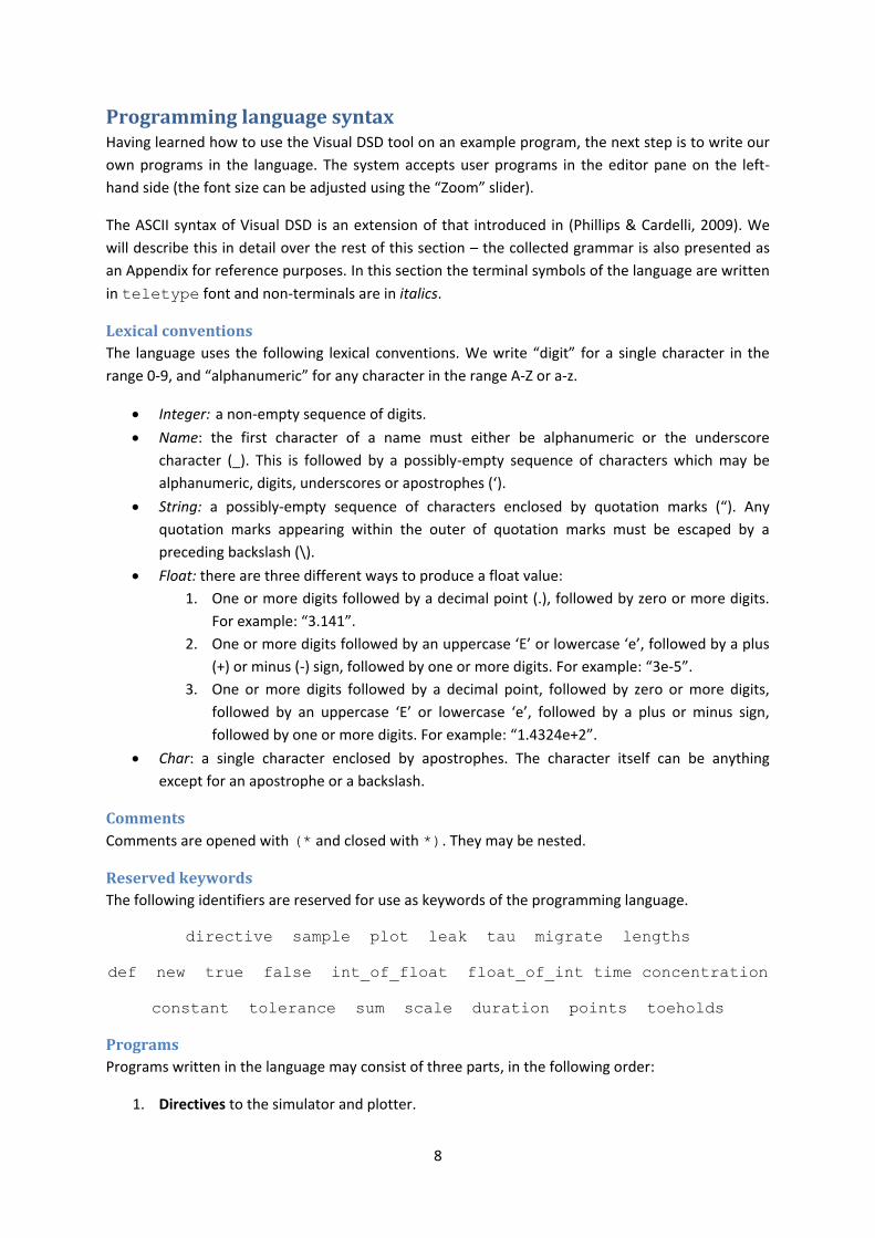
The “Options” menu allows further configuration of the semantics and behaviour of the Visual DSD

language itself. The “Unproductive” checkbox toggles the inclusion of reactions of repeated toehold

binding and unbinding. These reversible reactions go back and forth at a high rate and take up a lot

of simulator time without affecting the overall result of the simulation greatly. An example of such a

reaction is the following (not taken from the catalytic gate example):

This reaction is deemed unproductive because no other reactions can happen involving the molecule

on the right-hand side (since none of the domains next to the toehold match up). Removing these

spurious reactions slightly reduces the accuracy of the stochastic simulation but can make the

simulation algorithm run considerably faster. Note that the “Unproductive” checkbox is greyed out

when “Infinite” is selected from the “Compilation” menu because it has no effect under that

semantic model.

The “Leaks” checkbox toggles the inclusion of leak reactions, which are a form of unwanted

interference between strands and gates – see the “Leak model” section below for a brief

explanation. The “Declare domains” checkbox allows the user to enable stricter syntax checking

which produces an error if a domain is used without having first been declared using the “new”

keyword. This can be helpful when debugging programs, as a mistyped domain can be hard to detect

and can significantly alter the behaviour of the system.

7

Finally, the “Polymers” checkbox enables additional reduction rules which allow DNA gates to bind

together to form polymers of potentially unbounded length. This is a new feature that is not present

in the language described in (Phillips & Cardelli, 2009). The following reaction is an example of DNA

polymerization in which two gates bind together to form a stable complex.

However, it is also possible to write DSD programs involving polymerization where the full reaction

graph is infinite. For example, the following program

directive sample 10.0 100

( 10 * {t^*}[a]:[b]<t^ a> )

produces various reactions, including the following. Clearly this DNA polymer could grow indefinitely

if we kept supplying it with monomers to join onto the chain.

Attempting to compile such a program to chemical reactions using the standard DSD compiler will

cause the compiler to loop indefinitely as it attempts to discover the entire reaction graph, which is

infinite. It is recommended to use the JIT simulator (described in the “Simulation algorithms in Visual

DSD” section below) when dealing with programs that involve polymer reactions. To alert users to

this problem, the system produces an error message if a polymerization reaction is detected when

the “Polymers” checkbox is unchecked, as follows.

This error message also appears if an unproductive polymerization reaction is detected when the

“Unproductive” checkbox is checked but the “Polymers” checkbox is not.

The “States” tab on the right-hand side (and its four sub-tabs, the “Graph”, “Text”, “PRISM” and

“Visualise” tabs) are populated with output when the “Analyse” button is clicked. This computes the

continuous time Markov chain of the system and displays it in various ways for analysis and output:

see the “State space analysis” section below for more details.

8

Programming language syntax Having learned how to use the Visual DSD tool on an example program, the next step is to write our

own programs in the language. The system accepts user programs in the editor pane on the left-

hand side (the font size can be adjusted using the “Zoom” slider).

The ASCII syntax of Visual DSD is an extension of that introduced in (Phillips & Cardelli, 2009). We

will describe this in detail over the rest of this section – the collected grammar is also presented as

an Appendix for reference purposes. In this section the terminal symbols of the language are written

in teletype font and non-terminals are in italics.

Lexical conventions

The language uses the following lexical conventions. We write “digit” for a single character in the

range 0-9, and “alphanumeric” for any character in the range A-Z or a-z.

Integer: a non-empty sequence of digits.

Name: the first character of a name must either be alphanumeric or the underscore

character (_). This is followed by a possibly-empty sequence of characters which may be

alphanumeric, digits, underscores or apostrophes (‘).

String: a possibly-empty sequence of characters enclosed by quotation marks (“). Any

quotation marks appearing within the outer of quotation marks must be escaped by a

preceding backslash (\).

Float: there are three different ways to produce a float value:

1. One or more digits followed by a decimal point (.), followed by zero or more digits.

For example: “3.141”.

2. One or more digits followed by an uppercase ‘E’ or lowercase ‘e’, followed by a plus

(+) or minus (-) sign, followed by one or more digits. For example: “3e-5”.

3. One or more digits followed by a decimal point, followed by zero or more digits,

followed by an uppercase ‘E’ or lowercase ‘e’, followed by a plus or minus sign,

followed by one or more digits. For example: “1.4324e+2”.

Char: a single character enclosed by apostrophes. The character itself can be anything

except for an apostrophe or a backslash.

Comments

Comments are opened with (* and closed with *). They may be nested.

Reserved keywords

The following identifiers are reserved for use as keywords of the programming language.

directive sample plot leak tau migrate lengths

def new true false int_of_float float_of_int time concentration

constant tolerance sum scale duration points toeholds

Programs

Programs written in the language may consist of three parts, in the following order:

1. Directives to the simulator and plotter.

9

2. Declarations of values, global domains and modules.

3. A process to run, which contains the species and their initial populations.

A program must contain a process and may contain directives and/or declarations.

Program ::= Directives Declarations Process | Directives Process | Declarations Process | Process

Directives and Declarations stand for possibly-empty sequences of the Directive and Declaration

non-terminals, which are described below.

Directives

Directives are instructions to the Visual DSD simulator and data plotter.

Directive ::= directive duration Float | directive duration Float points Integer | directive sample Float | directive sample Float Integer

| directive scale Float | directive concentration String | directive time String | directive plot Plots | directive leak Float | directive tau Float | directive migrate Float | directive lengths Integer Integer | directive tolerance Float | directive toeholds Float Float

“Duration” directives tell the simulator how long to run for (as a floating-point number). Optionally

they may include a “Points” value with an integer value which specifies how many samples of the

species populations to take during that time (if none is provided, the default is to sample species

populations after every reaction, which can produce a large number of data points). The “Sample”

directives are an alternative syntax which has the same behaviour and is included for backwards

compatibility. Increasing the number of data points in the same period of simulation time produces

more fine-grained results but the display may be less responsive. Similarly, if the number of data

points stays constant but the simulation time is extended (or shortened), the resulting plot will be

less (or more) detailed. If no such directives are provided, the default behaviour is to run the

simulation for 1000 time units and take 10,000 samples of the species populations.

“Scale” directives allow the stochastic simulator to scale up from molar concentrations to

populations of individuals. Concentrations are scaled by simply multiplying by the factor and the

rates of binary reactions are modified following Section 4.2 of (Cardelli, 2008). Thus the user does

not have to worry about the details involved in switching between continuous and discrete

simulation methods (see below). The scale factor is 1.0 by default. The scale factor also modifies the

tolerance parameter of the deterministic simulator, as described below. See the “Populations and

concentrations” section below for further details.

10

“Concentration” directives allow one to specify the assumed unit of concentrations. It will be printed

on the y-axis of simulation plots when the simulator is run in deterministic mode. It will also feature

in the summary information in the “Text” tab. The default concentration units are nanomolar (nM).

“Time” directives allow one to specify the assumed unit of time. It will be printed on the x-axis of

simulation plots. The default time units are seconds (s).

“Plot” directives tell the system which populations to sample at each time point. If no “Plot”

directive is supplied, the system will sample the populations of all species at each time point.

Plots ::= String | Gate | Strand | sum( Plots ) | sub( Plot ; Plot ) | diff( Plot ; Plot ) | div( Plot ; Plot ) | Plots ; Plots

Plots is a semicolon-separated list of strand and gate species to plot. If any of the species contain the

underscore character (_) this is interpreted as a wildcard which can match against a single domain,

causing multiple species to be plotted. For example, the pattern <_ s t> will match against <u

s t> and <v s t> but not against <u v s t>. “Plot” directives may also include quoted

strings – in this case the decision of whether to plot is based on an exact string matching on the

names of species. This can be useful when dealing with locally restricted domains, as these are

automatically renamed by the system. It is also possible to plot simple arithmetic functions on

species populations, such as the sum of the populations of multiple species, using the “sum”

keyword followed by the species enclosed in brackets. For a given pair of plot species P1 and P2 one

can also plot the population of P1 minus the population of P2 (using “sub”), the difference (using

“diff”) or the ratio of P1 to P2 (using “div”).

The other directives allow the user to set the values of certain constants used by the system.

“Leak” directives set the rate of a leak reaction (default is 10-9 nM−1s−1).

“Tau” directives set the rate of a tau reaction in the Finite semantics (default is 0.1126 s−1).

“Migrate” directives set the rate of branch migration across a single nucleotide (default is

8000 s−1). The branch migration rate for a domain of length L is given by r/L2, where r is the

single nucleotide migration rate set by the directive.

“Lengths” directives set default values for the lengths of toeholds and long domains. For the

purpose of computing rate constants, all long domains are assumed to have the same

length, which is set using the “lengths” directive. The code “directive lengths 5

15” assigns a length of 5nt to toeholds and 15nt to long domains (the default values are

6nt for toeholds and 20nt for long domains). The value provided for toeholds must be

greater than that provided for specificity domains or the system will raise an error. Currently

the assigned default length for toehold domains is not used to calculate rates. Instead the

user may set toehold binding and unbinding rates directly on a per-toehold basis. Note that

specific nucleotide sequences are not currently used when computing rate constants.

11

“Tolerance” directives specify the tolerance parameter of the deterministic simulator, which

provides a tradeoff between computational cost and smoothness of the resulting solution.

The default value is 10-6. It is crucial to choose a tolerance value which reflects the

populations and reaction rates of the system in question, or the performance of the

deterministic simulator may suffer. Note that the tolerance is multiplied by the scale factor

in an attempt to maintain a reasonable value with respect to the species populations.

“Toeholds directives” specify the default binding and unbinding rates (in that order) for

domains which are declared without explicit rates. The default values are 3.0*10-4 nM−1s−1

for the binding rate and 0.1126 s−1 for the unbinding rate.

Declarations

These introduce new module definitions, globally-defined domains and value assignments.

Declaration ::= def Name ()= Process | def Name ( Parameters )= Process | new Name @ Value , Value | new Name | def Name = Value

The first two lines are for module declarations, which are written with the “def” keyword. A module

is simply a parameterised process. Here, Parameters stands for a non-empty, comma-separated list

of Names which are the parameters of that particular module. The grammar also permits a module

to have an empty parameter list. We will describe processes below. The name and parameters of a

module are bound within the body of that module and the name of the module is bound in the

remainder of the program.

A “new” declaration declares a new domain. This is global in the sense that the name of the domain

is bound in the rest of the program. Optionally, the domain may be annotated with two floating-

point values which explicitly state the binding and unbinding rates of the domain, respectively. If

these are omitted, the default rates set by the “toeholds” directive are used (if no such directive

is present in the program, the defaults are 3.0*10-4 nM−1s−1 for binding and 0.1126 s−1 for unbinding).

It is worth pointing out that not all of the domains used in a program need to be declared globally in

this way. If the system detects an undeclared domain in the program then it is assumed to have

these default binding and unbinding rates. This allows programs to remain short while allowing the

flexibility to modify the interaction rates of certain domains as needed. No units are supplied for the

rate values – it is up to the programmer to ensure that all rates are given in the same (implicit) units.

The unbinding rates are used in the Default semantic model (see below).

Value definitions (also written using “def”) assign a value to a name. Any subsequent uses of the

name will refer to this value, unless there is an intervening binding occurrence of the same name

(i.e. an instance of “def” or “new”). The system will raise an error if a name is used without having

first been bound to a value (unless the name is used as a domain, as mentioned above).

Processes

The core of Visual DSD is a process calculus tailored to modeling DNA interactions. The grammar of

processes is as follows.

12

Process ::= Value * Process | constant Process | constant Value * Process | Value * constant Process | Species | new Name @ Value , Value Process | new Name Process | ( Processes )

Processes ::= Process

| Process | Processes

The first four lines of the grammar allow the populations of certain processes to be specified (in each

case, the value should evaluate to an integer). The constant keyword specifies that the

population of a particular species should never change, even if it participates in reactions which

should consume that species. We will discuss the grammar of species themselves in detail below.

The “new” process declares a domain which has local scope, i.e. which can only be used within the

body of that process. As with globally-declared domains, these can have optional binding and

unbinding rates attached (otherwise, default rates are used as described above). This facility does

not add expressive power to the language but makes it easier to organize larger programs by re-

using the names of domains without mutual interference.

Finally, we can run multiple different kinds of processes in parallel using the vertical bar notation (|).

This is essential because molecules must be in parallel in order to react with each other. If two sets

of identical processes are placed in parallel, the system will notice and add up their populations to

produce a single population value for each species.

Species

The Visual DSD language allows various kinds of DNA molecules to be expressed. We present a brief

overview here – see (Phillips & Cardelli, 2009) for a more technical discussion of certain aspects, but

note that Visual DSD expands on the syntax from that paper.

We start with the most basic elements and work our way up. The language does not work at the

level of individual nucleotides – instead, the fundamental building blocks of species in Visual DSD are

DNA sequences. A sequence represents some finite section of DNA, comprising many nucleotides

(see below for a discussion on mapping domains to nucleotide sequences). We assume that distinct

sequences are sufficiently different that they do not interact, and that they do not possess any

secondary structure. The grammar for sequences in Visual DSD is as follows.

Sequence ::= Integer | Name | _

A Sequence is represented by a name, although this may actually be a number for convenience.

Hence a species such as <1 2 3> is valid, where 1, 2 and 3 denote different DNA sequences. The

underscore is permitted so that wildcards may be included in plotting directives (see above).

13

A Domain can either be a sequence or its Watson-Crick complement (obtained by reversing the

directionality of the nucleotide sequence then swapping C ↔ G and T ↔ A throughout). We denote

the complement of a sequence using an asterisk (*), so the grammar for domains is as follows.

Domain ::= Sequence | Sequence *

Toeholds are DNA domains which are sufficiently short that they can bind to (and unbind from) their

complementary strands quickly and easily. The basic syntax of a toehold domain is simply a domain

suffixed with a caret (^), but there is also the possibility of explicitly complementing the toehold

domain, as described above.

Toehold ::= Sequence ^ | Sequence ^ *

The explicit complementation operator is a new addition to the Visual DSD language. It was not

included in the syntax of (Phillips & Cardelli, 2009) because there it was assumed that the

complemented sequences were all on the lower strand of the DNA molecule. Our language provides

for greater flexibility, hence explicit complementation is required in the syntax. To convert programs

written in older versions of Visual DSD (v0.12 or before) to the new syntax, simply replace every

exposed toehold t^ by t^*.

We write Domains to stand for a non-empty sequence of Domain or Toehold domain elements,

separated by a space.

Domains ::= Domain | Toehold | Domain Domains | Toehold Domains

Domains are used to construct strands and more complicated DNA molecules. An UpperStrand

represents a single “upper” strand of DNA sequences and a LowerStrand represents a single “lower”

strand of DNA sequences. A Double represents an “upper” and a “lower” strand which are bound

due to Watson-Crick complementarity, as described above. Since these are all just lists of Domains

they must be distinguished by their ASCII syntax.

Double ::= [ Domains ]

UpperStrand ::= < Domains >

LowerStrand ::= { Domains }

In a double strand, we assume that the domains listed between the square brackets are the domains

on the upper strand, so a double strand written as [D1 D2* D3] would be visualized as follows,

where the small arrows at the top left and bottom right denote the 3’ ends of the DNA strands.

14

DNA gates are a key aspect of the strand displacement computational mechanism. A Gate is simply a

concatenation of one or more Segments of DNA.

Gate ::= Segment | Segment : Gate | Segment :: Gate

Overhangs ::= LowerStrand

| UpperStrand | LowerStrand UpperStrand | UpperStrand LowerStrand

Segment ::= Toehold

| LowerStrand | UpperStrand | Double | Double Overhangs | Overhangs Double | Overhangs Double Overhangs

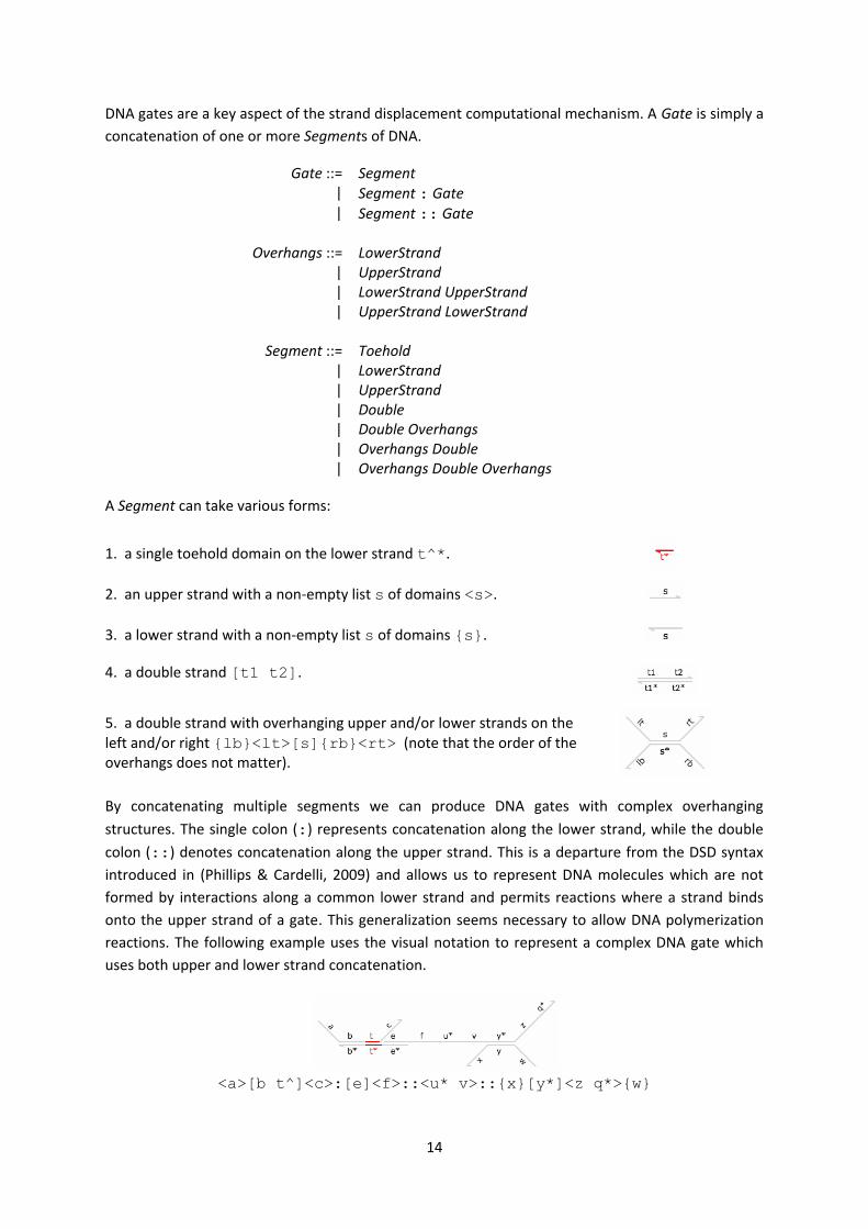
A Segment can take various forms:

1. a single toehold domain on the lower strand t^*.

2. an upper strand with a non-empty list s of domains <s>.

3. a lower strand with a non-empty list s of domains {s}.

4. a double strand [t1 t2].

5. a double strand with overhanging upper and/or lower strands on the left and/or right {lb}<lt>[s]{rb}<rt> (note that the order of the overhangs does not matter).

By concatenating multiple segments we can produce DNA gates with complex overhanging

structures. The single colon (:) represents concatenation along the lower strand, while the double

colon (::) denotes concatenation along the upper strand. This is a departure from the DSD syntax

introduced in (Phillips & Cardelli, 2009) and allows us to represent DNA molecules which are not

formed by interactions along a common lower strand and permits reactions where a strand binds

onto the upper strand of a gate. This generalization seems necessary to allow DNA polymerization

reactions. The following example uses the visual notation to represent a complex DNA gate which

uses both upper and lower strand concatenation.

<a>[b t^]<c>:[e]<f>::<u* v>::{x}[y*]<z q*>{w}

15

We impose a well-formedness criterion on Visual DSD programs that no long domain d and its

complement d* can be simultaneously exposed in the initial program. This suffices to ensure that no

molecules can be produced which could interact on their long domains, which preserves our key

assumption that all reactions are toehold-mediated.

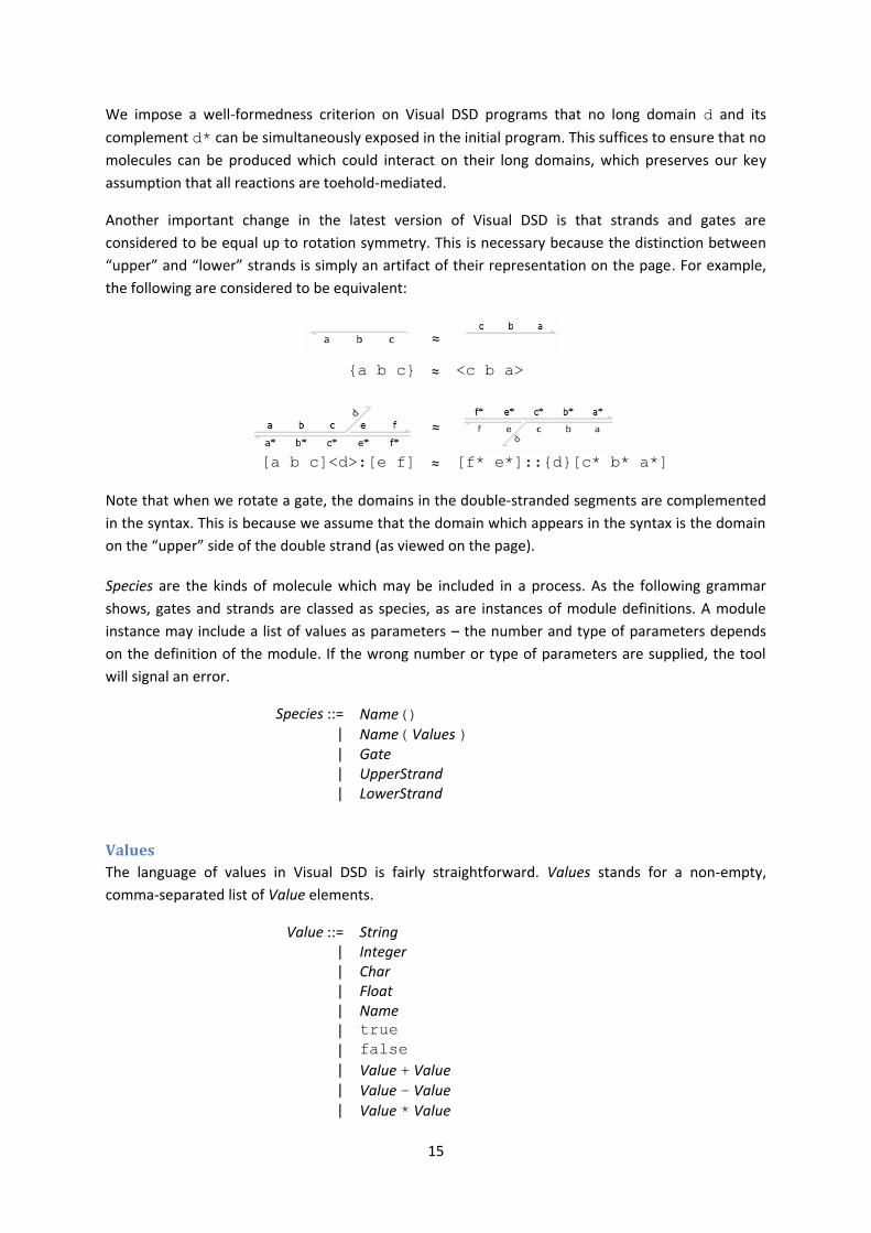
Another important change in the latest version of Visual DSD is that strands and gates are

considered to be equal up to rotation symmetry. This is necessary because the distinction between

“upper” and “lower” strands is simply an artifact of their representation on the page. For example,

the following are considered to be equivalent:

≈

{a b c} ≈ <c b a>

≈

[a b c]<d>:[e f] ≈ [f* e*]::{d}[c* b* a*]

Note that when we rotate a gate, the domains in the double-stranded segments are complemented

in the syntax. This is because we assume that the domain which appears in the syntax is the domain

on the “upper” side of the double strand (as viewed on the page).

Species are the kinds of molecule which may be included in a process. As the following grammar

shows, gates and strands are classed as species, as are instances of module definitions. A module

instance may include a list of values as parameters – the number and type of parameters depends

on the definition of the module. If the wrong number or type of parameters are supplied, the tool

will signal an error.

Species ::= Name() | Name( Values ) | Gate | UpperStrand | LowerStrand

Values

The language of values in Visual DSD is fairly straightforward. Values stands for a non-empty,

comma-separated list of Value elements.

Value ::= String | Integer | Char | Float | Name | true

| false

| Value + Value | Value – Value | Value * Value

16

| Value / Value | float_of_int Value | int_of_float Value | ( Value )

Values ::= Value | Value , Values

The base types String, Integer, Char, Float and Name follow the lexical conventions described above,

and the keywords true and false denote the usual Boolean constants. There are standard

arithmetic operators for addition, subtraction, multiplication and division. Both arguments must be

of the same type – either integers or floating point values. The float_of_int and

int_of_float functions explicitly convert between the two types, thus offering a way round this

restriction.

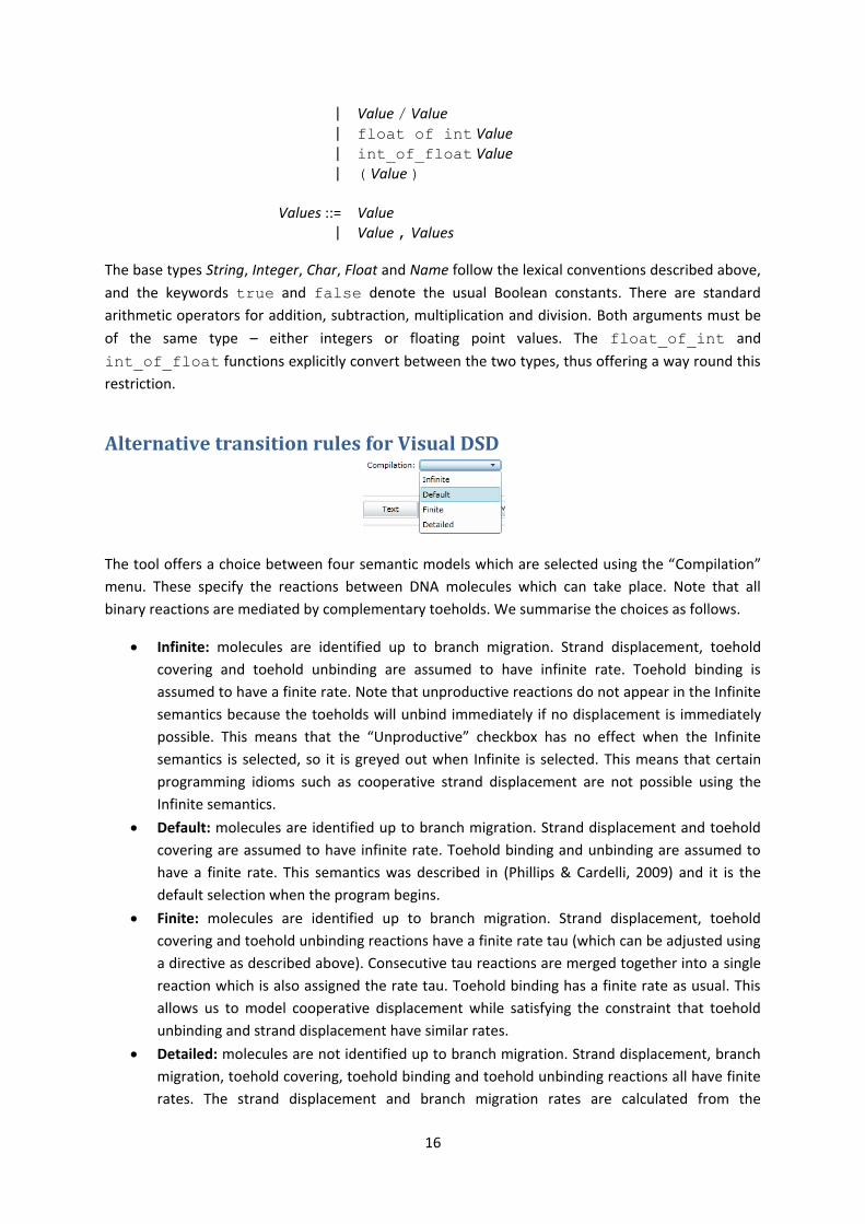
Alternative transition rules for Visual DSD

The tool offers a choice between four semantic models which are selected using the “Compilation”

menu. These specify the reactions between DNA molecules which can take place. Note that all

binary reactions are mediated by complementary toeholds. We summarise the choices as follows.

Infinite: molecules are identified up to branch migration. Strand displacement, toehold

covering and toehold unbinding are assumed to have infinite rate. Toehold binding is

assumed to have a finite rate. Note that unproductive reactions do not appear in the Infinite

semantics because the toeholds will unbind immediately if no displacement is immediately

possible. This means that the “Unproductive” checkbox has no effect when the Infinite

semantics is selected, so it is greyed out when Infinite is selected. This means that certain

programming idioms such as cooperative strand displacement are not possible using the

Infinite semantics.

Default: molecules are identified up to branch migration. Strand displacement and toehold

covering are assumed to have infinite rate. Toehold binding and unbinding are assumed to

have a finite rate. This semantics was described in (Phillips & Cardelli, 2009) and it is the

default selection when the program begins.

Finite: molecules are identified up to branch migration. Strand displacement, toehold

covering and toehold unbinding reactions have a finite rate tau (which can be adjusted using

a directive as described above). Consecutive tau reactions are merged together into a single

reaction which is also assigned the rate tau. Toehold binding has a finite rate as usual. This

allows us to model cooperative displacement while satisfying the constraint that toehold

unbinding and strand displacement have similar rates.

Detailed: molecules are not identified up to branch migration. Strand displacement, branch

migration, toehold covering, toehold binding and toehold unbinding reactions all have finite

rates. The strand displacement and branch migration rates are calculated from the

17

elementary migration rate and the assumed values for domain lengths (which can all be set

with directives) as described above.

Moving from the Infinite through to the Detailed semantic model the number of reactions in the

system increases dramatically and the computational cost of the compilation and simulation

processes increases also. The same is typically true when unproductive reactions are included.

The leak model The “Leaks” checkbox enables the simulation of certain kinds of interference between gates and

strands. These allow for a more realistic simulation of the actual behaviour of the system but may

increase the computational cost of the compilation and simulation phases.

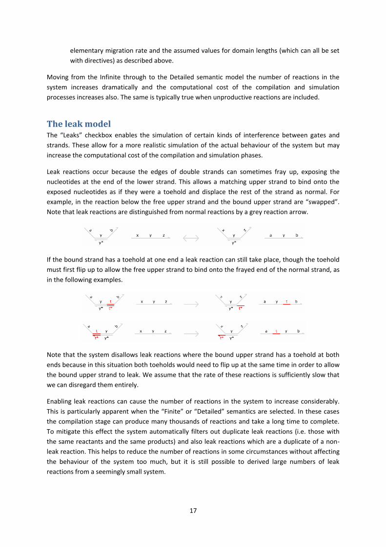
Leak reactions occur because the edges of double strands can sometimes fray up, exposing the

nucleotides at the end of the lower strand. This allows a matching upper strand to bind onto the

exposed nucleotides as if they were a toehold and displace the rest of the strand as normal. For

example, in the reaction below the free upper strand and the bound upper strand are “swapped”.

Note that leak reactions are distinguished from normal reactions by a grey reaction arrow.

If the bound strand has a toehold at one end a leak reaction can still take place, though the toehold

must first flip up to allow the free upper strand to bind onto the frayed end of the normal strand, as

in the following examples.

Note that the system disallows leak reactions where the bound upper strand has a toehold at both

ends because in this situation both toeholds would need to flip up at the same time in order to allow

the bound upper strand to leak. We assume that the rate of these reactions is sufficiently slow that

we can disregard them entirely.

Enabling leak reactions can cause the number of reactions in the system to increase considerably.

This is particularly apparent when the “Finite” or “Detailed” semantics are selected. In these cases

the compilation stage can produce many thousands of reactions and take a long time to complete.

To mitigate this effect the system automatically filters out duplicate leak reactions (i.e. those with

the same reactants and the same products) and also leak reactions which are a duplicate of a non-

leak reaction. This helps to reduce the number of reactions in some circumstances without affecting

the behaviour of the system too much, but it is still possible to derived large numbers of leak

reactions from a seemingly small system.

18

Note that Visual DSD does not currently support leak reactions which create DNA polymers by

binding two gate molecules together.

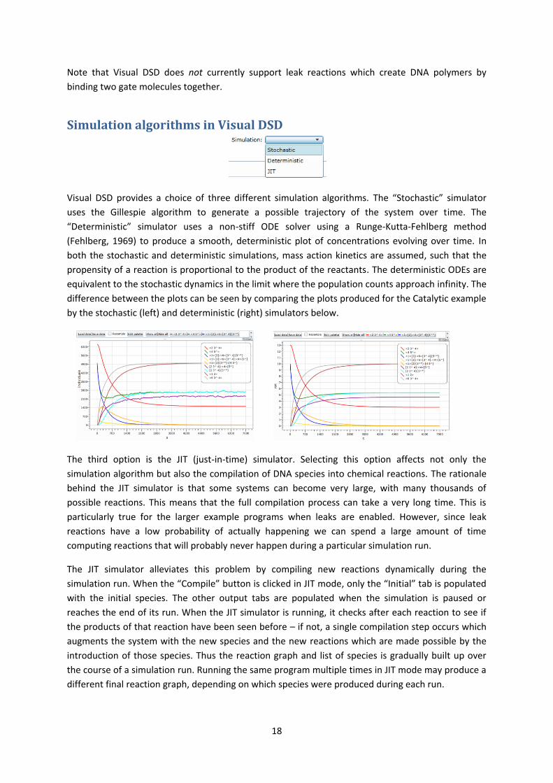
Simulation algorithms in Visual DSD

Visual DSD provides a choice of three different simulation algorithms. The “Stochastic” simulator

uses the Gillespie algorithm to generate a possible trajectory of the system over time. The

“Deterministic” simulator uses a non-stiff ODE solver using a Runge-Kutta-Fehlberg method

(Fehlberg, 1969) to produce a smooth, deterministic plot of concentrations evolving over time. In

both the stochastic and deterministic simulations, mass action kinetics are assumed, such that the

propensity of a reaction is proportional to the product of the reactants. The deterministic ODEs are

equivalent to the stochastic dynamics in the limit where the population counts approach infinity. The

difference between the plots can be seen by comparing the plots produced for the Catalytic example

by the stochastic (left) and deterministic (right) simulators below.

The third option is the JIT (just-in-time) simulator. Selecting this option affects not only the

simulation algorithm but also the compilation of DNA species into chemical reactions. The rationale

behind the JIT simulator is that some systems can become very large, with many thousands of

possible reactions. This means that the full compilation process can take a very long time. This is

particularly true for the larger example programs when leaks are enabled. However, since leak

reactions have a low probability of actually happening we can spend a large amount of time

computing reactions that will probably never happen during a particular simulation run.

The JIT simulator alleviates this problem by compiling new reactions dynamically during the

simulation run. When the “Compile” button is clicked in JIT mode, only the “Initial” tab is populated

with the initial species. The other output tabs are populated when the simulation is paused or

reaches the end of its run. When the JIT simulator is running, it checks after each reaction to see if

the products of that reaction have been seen before – if not, a single compilation step occurs which

augments the system with the new species and the new reactions which are made possible by the

introduction of those species. Thus the reaction graph and list of species is gradually built up over

the course of a simulation run. Running the same program multiple times in JIT mode may produce a

different final reaction graph, depending on which species were produced during each run.

19

Using the JIT simulator offers significant practical advantages when handling large-scale systems

such as those which include leak reactions. In many cases, simulating a system with leaks using the

JIT simulator is comparable in speed to simulating that system without leaks using the stochastic

simulator. Furthermore, the JIT simulator is essential when working with systems which have the

potential to form DNA polymer molecules of unbounded size. In these cases the JIT simulator only

compiles the subset of reactions which are reachable from a species that has been created during

the simulation run, as opposed to the full (infinite) reaction graph. Thus the JIT simulator may be the

only way to run DNA polymer programs without causing the compiler to loop forever.

Populations and concentrations In Visual DSD, quantities of DNA complexes are specified as molar concentrations, which denote the

number of moles per unit volume. The units of concentration can be set by the concentration

directive. For example, directive concentration "M" sets the units of concentration to

molar. The default units are nanomolar (nM), where 1nM = 10-9 mol/L.

In order to perform a stochastic simulation, concentrations must be converted to numbers of

individuals. This can be achieved using the following equation:

n = c·V·NA

where n is the number of individuals, c is the molar concentration, V is the volume and NA is

Avogadro's constant, which denotes the number of individuals per mole of substance (approximately

6.02214×1023 mol−1). The function x denotes the rounding up of x to its nearest natural number.

Thus, in order to convert a concentration into a number of individuals, it is sufficient to multiply the

concentration by a scale factor s = V·NA, which denotes the number of individuals per unit

concentration. Essentially, this corresponds to choosing a volume V such that the number of

individuals is equal to s for one unit of concentration. For example, a scale factor of 50 corresponds

to choosing a volume that is 50 times the volume occupied by a single individual. The units of the

scale factor are assumed to be the inverse of the units of concentration, and are given as nM−1 by

default. Note that the conversion from concentrations to individuals is achieved using a scale factor s

rather than specifying a volume V directly, since it is difficult to choose a volume such that the

number of individuals is a natural number. The scale factor can be set by the scale directive,

where the default scale factor is 1.0.

The choice of deterministic (continuous) or stochastic (discrete) simulation is also manifested in the

units for the simulation plot. The vertical axis of the plot has units of individuals for stochastic

simulation, and units of concentration for deterministic simulation. Note that the units for rate

constants are assumed to be consistent with the units for time and concentration. For example, if

the units for time are s and the units for concentration are nM, then the units for the bimolecular

rate constants are assumed to be nM−1s−1, and the units for the unimolecular rate constants are

assumed to be s−1. Once a suitable scale factor has been selected, in order to perform a stochastic

simulation the molar concentrations are multiplied by the scale factor, while the concentration-

dependent rates are divided by the scale factor. For example, if the scale factor is 100 nM−1 then a

concentration-dependent rate of 0.4 nM−1s−1 is converted to a stochastic rate of 0.004 s−1 for

20

simulation. Additional details on converting between populations and concentrations can be found

in Section 4.2 of (Cardelli, 2008), including specific conversion rules for homodimerization reactions.

State space analysis Visual DSD can also compute the graph of all reachable states for the system from the initial

molecules. This is useful for debugging individual components and for verifying larger completed

designs. Note, however, that if there are many possible interleavings of the reactions the state graph

can be very large and this can take a long time to compute – in such cases, the computation can be

stopped using the “Pause” button. When the “Analysis” button is clicked the system computes the

continuous time Markov chain and populates the four sub-tabs of the “States” tab on the right-hand

side. Note that the state-space analyser always uses JIT compilation as it calculates the state space,

regardless of what is selected in the “Simulation” menu.

The “Graph” tab displays the set of reachable states as a graph, using a similar graph display to that

used for the chemical reaction network. Each reachable state is represented as a node of the graph,

and every possible reaction is represented as an edge. There are some additional statistics along the

bottom on the size of the state space, and a checkbox to “Draw images” which toggles between

graphical and textual views of the populations within each node. The initial state of the system is

highlighted with a thick black border (on the left in the image below) and any terminal states (that is,

states from which no reactions are possible) are highlighted with a thick red border (on the right in

the image below).

The “Text” tab displays a textual summary of the state space, with statistics on the size of the state

space (numbers of states, transitions and terminal states), the populations of species present in the

initial state and any terminal states, and the minimum and maximum populations of each species in

the state graph. The “PRISM” tab displays code generated for the PRISM model checker which

corresponds to the state space of the system. This can be used to verify properties of the DNA circuit

using probabilistic model checking. Finally, the “Visualise” tab presents a visual summary of the

populations of species present in the initial state and any terminal states.

21

Implementing domains as nucleotide sequences Visual DSD allows for domains to be compiled into nucleotide sequences, providing a template for

implementation of systems in DNA in the laboratory. The “DNA” tab on the left-hand side of the

interface allows the user to enter the sequences that are used to implement toehold and specificity

domains.

The windows for toehold and specificity sequences are preloaded with toehold domain sequences

from the Appendix to (Zhang, Turberfield, Yurke, & Winfree, 2007) and specificity sequences which

were generated by Qian for (Qian & Winfree, 2009). The user can edit these and enter their own

additional DNA sequences but there are some constraints:

The only characters allowed are upper case A, C, G and T.

Only one sequence is permitted per line.

The same sequence cannot be repeated.

Toehold sequences cannot be longer than 9 nucleotides.

Specificity sequences cannot be shorter than 10 nucleotides.

The tool does not perform any other sanity-checking than this, so further investigation of the

sequences may be required to verify that they are appropriate for use in experiments. If a large

number of DNA sequences is supplied, these sanity checks can slow down the compilation process.

The “Check sequences” option allows the user to disable the checks for repeated sequences and for

the lengths of toehold and specificity sequences, to speed up compilation. These checks can be

safely disabled for the preloaded sequences that come with the Visual DSD tool.

The sequences are output (in order) into the “Domains” tab when the “Compile” button is clicked. If

the program contains more domains than there are available sequences, the system indicates this in

the “Domains” tab, as shown below. The “Domains” tab also shows explicitly which end of the DNA

sequence is the 3’ end and which is the 5’ end.

If the “Show Nucleotides” checkbox is ticked, the mapping of domains to nucleotide sequences is

used to display those sequences in the graphical representations of molecules in the “Initial” tab and

in the “Species”, “Reactions” and “Graph” tabs. When the checkbox is clicked, these tabs are

22

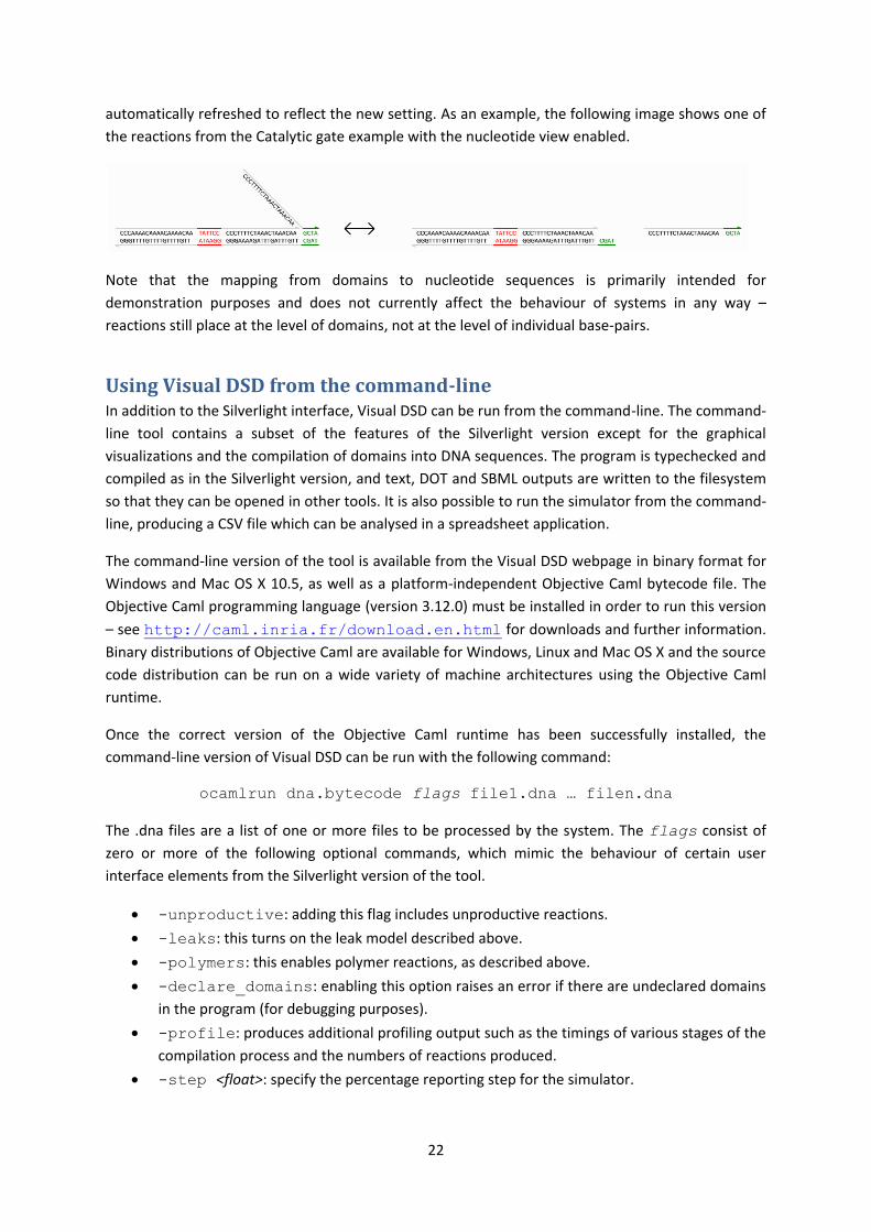
automatically refreshed to reflect the new setting. As an example, the following image shows one of

the reactions from the Catalytic gate example with the nucleotide view enabled.

Note that the mapping from domains to nucleotide sequences is primarily intended for

demonstration purposes and does not currently affect the behaviour of systems in any way –

reactions still place at the level of domains, not at the level of individual base-pairs.

Using Visual DSD from the command-line In addition to the Silverlight interface, Visual DSD can be run from the command-line. The command-

line tool contains a subset of the features of the Silverlight version except for the graphical

visualizations and the compilation of domains into DNA sequences. The program is typechecked and

compiled as in the Silverlight version, and text, DOT and SBML outputs are written to the filesystem

so that they can be opened in other tools. It is also possible to run the simulator from the command-

line, producing a CSV file which can be analysed in a spreadsheet application.

The command-line version of the tool is available from the Visual DSD webpage in binary format for

Windows and Mac OS X 10.5, as well as a platform-independent Objective Caml bytecode file. The

Objective Caml programming language (version 3.12.0) must be installed in order to run this version

– see http://caml.inria.fr/download.en.html for downloads and further information.

Binary distributions of Objective Caml are available for Windows, Linux and Mac OS X and the source

code distribution can be run on a wide variety of machine architectures using the Objective Caml

runtime.

Once the correct version of the Objective Caml runtime has been successfully installed, the

command-line version of Visual DSD can be run with the following command:

ocamlrun dna.bytecode flags file1.dna … filen.dna

The .dna files are a list of one or more files to be processed by the system. The flags consist of

zero or more of the following optional commands, which mimic the behaviour of certain user

interface elements from the Silverlight version of the tool.

-unproductive: adding this flag includes unproductive reactions.

-leaks: this turns on the leak model described above.

-polymers: this enables polymer reactions, as described above.

-declare_domains: enabling this option raises an error if there are undeclared domains

in the program (for debugging purposes).

-profile: produces additional profiling output such as the timings of various stages of the

compilation process and the numbers of reactions produced.

-step <float>: specify the percentage reporting step for the simulator.

23

-simulate <string>: if this is enabled the system is simulated after it has been compiled,

and the results of the simulation are written into a CSV file. As in the Silverlight interface

there are three possible choices for the simulator mode: Stochastic, Deterministic

and JIT.

-semantics <string>: this modifies the semantic model used for computing the set of

reactions. As in the Silverlight interface, the choices are Infinite, Default, Finite

and Detailed. The default semantic model is Default.

The command-line arguments are the same in the command-line version compiled using F#, except

that “ocamlrun” is not needed in the command-line invocation.

24

Bibliography Cardelli, L. (2008). On process rate semantics. Theoretical Computer Science , 391 (3), 190-215.

Fehlberg, E. (1969). Low-order classical Runge-Kutta formulas with stepsize control. NASA Technical

Report R-315.

Huang, C.-Y. F., & Ferrel, J. E. (1996). Ultrasensitivity of the mitogen-activated protein kinase

cascade. PNAS , 93, 10078-10083.

Phillips, A., & Cardelli, L. (2009). A programming language for composable DNA circuits. Journal of

the Royal Society Interface .

Qian, L., & Winfree, E. (2009). A simple DNA gate motif for synthesizing large-scale circuits. In G. A.,

F. C. Simmel, & P. Sosik (Ed.), DNA 14. LNCS 5347, pp. 70-89. Springer-Verlag.

Zhang, D. Y., & Winfree, E. (2009). Control of DNA strand displacement kinetics using toehold

exchange. J. Am. Chem. Soc. , 131, 17303-17314.

Zhang, D. Y., Turberfield, A. J., Yurke, B., & Winfree, E. (2007). Engineering entropy-driven reactions

and networks catalyzed by DNA. Science , 318, 1121-1125.

25

Appendix: Collected summary of the Visual DSD language

Grammar

The full grammar of Visual DSD programs is as follows. Terminal symbols of the language are written

in teletype font and non-terminals are in italics.

Program ::= Directives Declarations Process A program must contain a process to run and may optionally contain directives and/or declarations.

| Directives Process | Declarations Process | Process

Directive ::= directive duration Float End time for simulation, with

optional number of datapoints. | directive duration Float

points Integer | directive sample Float End time for simulation, with

optional number of datapoints. | directive sample Float Integer | directive scale Float Specify a scaling factor.

| directive concentration CU Specify concentration units.

| directive time TU Specify time units.

| directive plot Plots Which species to plot.

| directive leak Float Rate of leak reactions.

| directive tau Float Rate of tau reactions.

| directive migrate Float Elementary migration rate.

| directive lengths Integer Integer Default domain lengths.

| directive tolerance Float Specify ODE solver tolerance.

| directive toeholds Float Float Default toehold reaction rates.

Directives ::= Directive Single directive

| Directive Directives Multiple directives

Plots ::= String Plot exact string match only | Gate Gate species to plot | Strand Strand species to plot | sum( Plots ) Plot sum of populations

| sub( Plot ; Plot ) Plot population subtraction

| diff( Plot ; Plot ) Plot population difference

| div( Plot ; Plot ) Plot population ratio

| Plots ; Plots Plot multiple populations

Declaration ::= def Name ()= Process Module definition

| def Name ( Parameters )= Process Module definition

| new Name @ Value , Value Global channel with rates

| new Name Global channel (default rates)

| def Name = Value Value assignment

Declarations ::= Declaration Single declaration

| Declaration Declarations Multiple declarations

Parameters ::= Name Single parameter | Name , Parameters Comma-separated parameters

26

Value ::= String String

| Integer Integer | Char Single character | Float Floating point | Name Name | true True | false False | Value + Value Addition

| Value – Value Subtraction

| Value * Value Multiplication

| Value / Value Division

| float_of_int Value Convert integer to float

| int_of_float Value Convert float to integer

| ( Value ) Parenthesised value

Values ::= Value Single value

| Value , Values Comma-separated values

Process ::= Value * Process Repetition

| constant Process Constant population

| constant Value * Process Constant repetition

| Value * constant Process Repeated constant

| Species Species | new Name @ Value , Value Process Restriction with rates

| new Name Process Restriction (default rates)

| ( Processes ) Parallel processes

Processes ::= Process Single process

| Process | Processes Parallel processes

Species ::= Name() Module instance

| Name( Values ) Module instance

| Gate Gate | UpperStrand Upper strand | LowerStrand Lower strand

Gate ::= Segment Single segment

| Segment : Gate Lower strand concatenation

| Segment :: Gate Upper strand concatenation

Segment ::= Toehold Lower toehold

| LowerStrand Lower strand segment | UpperStrand Upper strand segment | Double Double strand | Double Overhangs Double with right overhang(s) | Overhangs Double Double with left overhang(s) | Overhangs Double Overhangs Double with both overhang(s)

Overhangs ::= LowerStrand Lower overhang

| UpperStrand Upper overhang

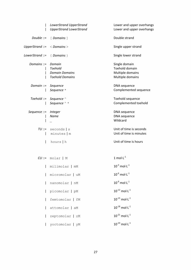
27

| LowerStrand UpperStrand Lower and upper overhangs | UpperStrand LowerStrand Lower and upper overhangs

Double ::= [ Domains ] Double strand

UpperStrand ::= < Domains > Single upper strand

LowerStrand ::= { Domains } Single lower strand

Domains ::= Domain Single domain

| Toehold Toehold domain | Domain Domains Multiple domains | Toehold Domains Multiple domains

Domain ::= Sequence DNA sequence

| Sequence * Complemented sequence

Toehold ::= Sequence ^ Toehold sequence

| Sequence ^ * Complemented toehold

Sequence ::= Integer DNA sequence

| Name DNA sequence | _ Wildcard

TU ::= seconds | s Unit of time is seconds

| minutes | m Unit of time is minutes

| hours | h Unit of time is hours

CU ::= molar | M 1 mol∙L-1

| milimolar | mM 10-3 mol∙L-1

| micromolar | uM 10-6 mol∙L-1

| nanomolar | nM 10-9 mol∙L-1

| picomolar | pM 10-12 mol∙L-1

| femtomolar | fM 10-15 mol∙L-1

| attomolar | aM 10-18 mol∙L-1

| zeptomolar | zM 10-21 mol∙L-1

| yoctomolar | yM 10-24 mol∙L-1

28

Lexical conventions

The language uses the following lexical conventions. We write “digit” for a single character in the

range 0-9, and “alphanumeric” for any character in the range A-Z or a-z.

Integer: a non-empty sequence of digits.

Name: the first character of a name must either be alphanumeric or the underscore

character (_). This is followed by a possibly-empty sequence of characters which may be

alphanumeric, digits, underscores or apostrophes (‘).

String: a possibly-empty sequence of characters enclosed by quotation marks (“). Any

quotation marks appearing within the outer of quotation marks must be escaped by a

preceding backslash (\).

Float: there are three different ways to produce a float value:

1. One or more digits followed by a decimal point (.), followed by zero or more digits.

For example: 3.141.

2. One or more digits followed by an uppercase ‘E’ or lowercase ‘e’, followed by a plus

(+) or minus (-) sign, followed by one or more digits. For example: 3e-5.

3. One or more digits followed by a decimal point, followed by zero or more digits,

followed by an uppercase ‘E’ or lowercase ‘e’, followed by a plus or minus sign,

followed by one or more digits. For example: 1.4324e+2.

Char: a single character enclosed by apostrophes. The character itself can be anything

except for an apostrophe or a backslash.

Comments

Comments are opened with (* and closed with *). They may be nested.

Reserved keywords

The following identifiers are reserved for use as keywords of the programming language.

directive sample plot leak tau migrate lengths

def new true false int_of_float float_of_int time concentration

constant tolerance sum scale duration points toeholds