Visual Hypothesis Tests in Multivariate Linear Models:The heplots Package for R

John FoxMcMaster University

Michael FriendlyYork University

Georges MonetteYork University

6 Februrary 2007

Abstract

Hypothesis-error (or “HE”) plots, introduced by Friendly (2006, 2007), permit the visualization ofhypothesis tests in multivariate linear models by representing hypothesis and error matrices of sums ofsquares and cross-products as ellipses. This paper describes the implementation of these methods in R,as well as their extension, for example from two to three dimensions and by scaling hypothesis ellipsesand ellipsoids in a natural manner relative to error. The methods, incorporated in the heplots packagefor R, exploit new facilities in the car package for testing linear hypotheses in multivariate linear modelsand for constructing MANOVA tables for these models, including models for repeated measures.

1 IntroductionThis paper introduces the heplots package for R, which implements and extends the methods described inFriendly (2006, 2007) for visualizing hypothesis tests in multivariate linear models. The paper begins with abrief description of multivariate linear models; proceeds to explain how dispersion matrices can be representedby ellipses or ellipsoids; describes new facilities in the car package (associated with Fox, 2002) for testinglinear hypotheses in multivariate linear models and for constructing multivariate analysis-of-variance tables;and illustrates the use of the functions in the heplots package for two and three-dimensional visualizationof hypothesis tests in multivariate analysis of variance and regression.

2 Multivariate Linear ModelsThe univariate linear model

y = Xβ + ε (1)

is surely the most familiar of statistical models. In Equation 1, y is an n× 1 column vector of observationson a response variable; X is an n × p model matrix of full column rank that is either fixed or, if random,independent of the n × 1 vector of errors ε; and the p × 1 vector of regression coefficients β is to beestimated from the data.. As is also familiar, under the standard assumptions that the errors are normallyand independently distributed with zero expectations and common variance, εi ∼ NID(0, σ2) or equivalentlyε ∼ Nn(0, σ

2In), the least squares estimator,bβ = (XTX)−1XTy

is the maximum-likelihood estimator of β. Here, Nn denotes the multivariate-normal distribution for nvariables, 0 is the n× 1 zero vector, and In is the order-n identity matrix.In the multivariate linear model (e.g., Timm, 1975),

Y = XB+E

the response vector y is replaced by an n×m matrix of responses Y, where each column represents a distinctresponse variable, B is a p×m matrix of regression coefficients, and E is an n×m matrix of errors. Under the

1

assumption that the rows of E are independent, and that each row is multivariately normally distributed withzero expectation and common covariance matrix, εTi ∼ Nn(0,Σ) or equivalently vec(E) ∼ Nnp(0, In ⊗Σ),the least squares estimator bB = (XTX)−1XTY

is the maximum-likelihood estimator or B. Here, the 0 vectors are respectively of order n × 1 and np × 1,and ⊗ represents the Kronecker product.Hypothesis tests for multivariate linear models also closely parallel those for univariate linear models.

Consider the linear hypothesisH0: Lβ = 0

in the univariate linear model, where L is a q× p hypothesis matrix of rank q and 0 is the q× 1 zero vector.Under this hypothesis,

F0 =

bβTLT [L(XTX)−1LT ]−1LbβqbεTbε

n− p

=SSH/q

SSE/(n− p)

is distributed as F with q and n − p degrees of freedom. The quantity SSH = bβTLT [L(XTX)−1LT ]−1Lbβ

is the sum of squares for the hypothesis, bε = y −Xbβ is the vector of residuals, SSE = bεTbε is the sum ofsquares for error, and s2 = bεTbε/(n− p) is the estimated error variance. To test the analogous hypothesis inthe multivariate linear model,

H0: LB = 0 (2)

where 0 is now the q×m zero matrix, we compute the m×m hypothesis sum of squares and products matrix

SSPH = bBTLT [L(XTX)−1LT ]−1LbBand the m×m error sum of squares and products matrix

SSPE = bET bEwhere bE = Y − XbB is the matrix of residuals. Multivariate tests of the hypothesis are based on thes = min(q,m) nonzero latent roots λ1 > λ2 > · · · > λs of the matrix SSPH relative to the matrix SSPE ,that is, the values of λ for which

det(SSPH − λSSPE) = 0

These are also the ordinary latent roots of of SSPHSSP−1E , that is, the values of λ for which

det(SSPHSSP−1E − λIm) = 0

The corresponding latent vectors give a set of s orthogonal linear combinations of the responses that pro-duce maximal univariate F statistics for the hypothesis in Equation 2. The several commonly employedmultivariate test statistics are functions of the latent roots:

Pillai’s trace, TP =

pXj=1

λj1 + λj

Hotelling-Lawley trace, THL =Pp

j=1 λj

Wilks’s Lambda, Λ =

pYj=1

1

1 + λj

Roy’s maximum root, λ1

There is an F approximation to the null distribution of each of these test statistics.In a univariate linear model, it is common to provide F tests for each term in the model, summarized in

an analysis-of-variance (ANOVA) table. The hypothesis sums of squares for these tests can be expressed asdifferences in the error sums of squares for nested models. For example, dropping each term in the model

2

in turn and contrasting the resulting residual sum of squares with that for the full model produces so-calledType-III tests; adding terms to the model sequentially produces so-called Type-I tests; and testing each termafter all terms in the model with the exception of those to which it is marginal produces so-called Type-IItests. Closely analogous multivariate analysis-of-variable (MANOVA) tables can be formed similarly bytaking differences in error sum of squares and products matrices.In some contexts – for example, when the response variables represent repeated measures of the same

variable over time – it is also of interest to entertain a design and hypotheses on the response (see, e.g.,O’Brien and Kaiser, 1985). Such tests can be formulated by extending the linear hypothesis in Equation 2to

H0: LBP = 0

where the m× k matrix P provides contrasts in the responses.

3 Data Ellipses and EllipsoidsThe data ellipse, described by Dempster (1969) and Monette (1990), is a device for visualizing the relationshipbetween two variables, Y1 and Y2. Let D2

M (y) = (y − y)TS−1(y − y) represent the squared Mahalanobisdistance of the point y = (y1, y2)T from the centroid of the data y = (Y 1, Y 2)

T . The data ellipse Ec of sizec is the set of all points y with D2

M (y) less than or equal to c2:

Ec(y;S,y) ≡©y: (y − y)TS−1(y− y) ≤ c2

ª(3)

Here, S is the sample covariance matrix,

S =

Pni=1(y − y)T (y− y)

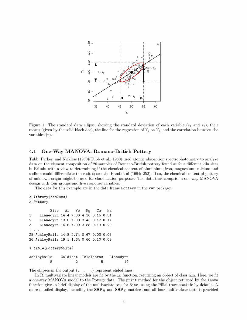
n− 1Selecting c = 1 produces the “standard” data ellipse, as illustrated in Figure 1: The perpendicular

“shadows” of the ellipse on the axes mark off twice the standard deviation of each variable; the regressionline for Y2 on Y1 intersects the points of vertical tangency on the boundary of the ellipse; and the correlationbetween the two variables is proportional to the length of the line from the bottom of the ellipse to the pointof vertical tangency at the right. Many other properties of correlation and regression can be visualized usingthe data ellipse (see, e.g., Monette, 1990).These properties of the data ellipse hold regardless of the joint distribution of the variables, but if the

variables are bivariate normal, then the data ellipse represents a contour of constant density in their jointdistribution. In this case, D2

M (y) has a large-sample χ2 distribution with 2 degrees of freedom, and so, for

example, taking c2 = χ22(0.95) = 5.99 ≈ 6 encloses approximately 95 percent of the data. Alternatively, insmall samples, we can take

c2 =2(n− 1)n− 2 F2,n−2 ≈ 2F2,n−2

but this typically makes little difference visually.The generalization of the data ellipse to more than two variables is immediate: Applying Equation 3 to

y = (y1, y2, y3)T , for example, produces a data ellipsoid in three dimensions. For m multivariate-normal

variables, selecting c2 = χ2m(1−α) encloses approximately 100(1−α) percent of the data. Again, for greaterprecision, we can use

c2 =m(n− 1)n−m

Fm,n−m ≈ mFm,n−m

4 Implementation of Tests for Multivariate Linear Models in thecar Package

Tests for multivariate linear models are implemented in the car package as S3 methods for the genericlinear.hypothesis and Anova functions, with Manova provided as a synonym for the latter. The Anovafunction computes partial (so-called “Types II and III”) hypothesis tests, as opposed to the anova function inthe stats package, which computes sequential (“Type-I”) tests; these tests coincide in one-way and balanceddesigns. Several examples of the use of these functions are given in this section.

3

35 40 45 50 55 60

7080

9010

011

012

013

0

Y1

Y 2

2 × s1

2× s2

2 × r× s2

-

Figure 1: The standard data ellipse, showing the standard deviation of each variable (s1 and s2), theirmeans (given by the solid black dot), the line for the regression of Y2 on Y1, and the correlation between thevariables (r).

4.1 One-Way MANOVA: Romano-British Pottery

Tubb, Parker, and Nickless (1980)(Tubb et al., 1980) used atomic absorption spectrophotometry to analyzedata on the element composition of 26 samples of Romano-British pottery found at four different kiln sitesin Britain with a view to determining if the chemical content of aluminium, iron, magnesium, calcium andsodium could differentiate those sites; see also Hand et al (1994: 252). If so, the chemical content of potteryof unknown origin might be used for classification purposes. The data thus comprise a one-way MANOVAdesign with four groups and five response variables.The data for this example are in the data frame Pottery in the car package:

> library(heplots)> Pottery

Site Al Fe Mg Ca Na1 Llanedyrn 14.4 7.00 4.30 0.15 0.512 Llanedyrn 13.8 7.08 3.43 0.12 0.173 Llanedyrn 14.6 7.09 3.88 0.13 0.20. . .25 AshleyRails 14.8 2.74 0.67 0.03 0.0526 AshleyRails 19.1 1.64 0.60 0.10 0.03

> table(Pottery$Site)

AshleyRails Caldicot IsleThorns Llanedyrn5 2 5 14

The ellipses in the output (. . .) represent elided lines.In R, multivariate linear models are fit by the lm function, returning an object of class mlm. Here, we fit

a one-way MANOVA model to the Pottery data. The print method for the object returned by the Anovafunction gives a brief display of the multivariate test for Site, using the Pillai trace statistic by default. Amore detailed display, including the SSPH and SSPE matrices and all four multivariate tests is provided

4

by the summary method for Anova.mlm objects (suppressing the univariate test for each response, which isgiven by default):

> pottery.mod <- lm(cbind(Al, Fe, Mg, Ca, Na) ~ Site, data=Pottery)> Anova(pottery.mod)

Type II MANOVA Tests: Pillai test statisticDf test stat approx F num Df den Df Pr(>F)

Site 3 1.5539 4.2984 15 60 2.413e-05 ***---Signif. codes: 0 ’***’ 0.001 ’**’ 0.01 ’*’ 0.05 ’.’ 0.1 ’ ’ 1

> # All 4 multivariate tests> summary(Anova(pottery.mod), univariate=FALSE, digits=4)

Type II MANOVA Tests:

Sum of squares and products for error:Al Fe Mg Ca Na

Al 48.2881 7.08007 0.60801 0.10647 0.58896Fe 7.0801 10.95085 0.52706 -0.15519 0.06676Mg 0.6080 0.52706 15.42961 0.43538 0.02762Ca 0.1065 -0.15519 0.43538 0.05149 0.01008Na 0.5890 0.06676 0.02762 0.01008 0.19929

------------------------------------------

Term: Site

Sum of squares and products for the hypothesis:Al Fe Mg Ca Na

Al 175.610 -149.296 -130.810 -5.8892 -5.3723Fe -149.296 134.222 117.745 4.8218 5.3259Mg -130.810 117.745 103.351 4.2092 4.7105Ca -5.889 4.822 4.209 0.2047 0.1548Na -5.372 5.326 4.711 0.1548 0.2582

Multivariate Tests: SiteDf test stat approx F num Df den Df Pr(>F)

Pillai 3.00 1.55 4.30 15.00 60.00 2.41e-05 ***Wilks 3.00 0.01 13.09 15.00 50.09 1.84e-12 ***Hotelling-Lawley 3.00 35.44 39.38 15.00 50.00 < 2e-16 ***Roy 3.00 34.16 136.64 5.00 20.00 9.44e-15 ***---Signif. codes: 0 ’***’ 0.001 ’**’ 0.01 ’*’ 0.05 ’.’ 0.1 ’ ’ 1

In this instance, we get the same test from the anova function in the standard stats package, because(as mentioned) for this one-factor design, the sequential test provided by anova is the same as the Type-IItest provided by default by Anova:

> anova(pottery.mod)

Analysis of Variance Table

Df Pillai approx F num Df den Df Pr(>F)(Intercept) 1 0.99 523.07 5 18 < 2.2e-16 ***

5

Site 3 1.55 4.30 15 60 2.413e-05 ***Residuals 22---Signif. codes: 0 ’***’ 0.001 ’**’ 0.01 ’*’ 0.05 ’.’ 0.1 ’ ’ 1

There is, therefore, strong evidence against the null hypothesis of no differences in mean vectors acrosssites.

4.2 Two-Way MANOVA: Plastic Film Data

For a slightly more complex example, we use textbook data from Johnson and Wichern (1992: 266) on anexperiment conducted to determine the optimum conditions for extruding plastic film. Three responses (tearresistance, film gloss, and opacity) were measured in relation to two factors: rate of extrusion (Low/High)and amount of an additive (Low/High). Again, the data are in the heplots package:

> Plastic

tear gloss opacity rate additive1 6.5 9.5 4.4 Low Low2 6.2 9.9 6.4 Low Low3 5.8 9.6 3.0 Low Low4 6.5 9.6 4.1 Low Low5 6.5 9.2 0.8 Low Low6 6.9 9.1 5.7 Low High7 7.2 10.0 2.0 Low High8 6.9 9.9 3.9 Low High9 6.1 9.5 1.9 Low High10 6.3 9.4 5.7 Low High11 6.7 9.1 2.8 High Low12 6.6 9.3 4.1 High Low13 7.2 8.3 3.8 High Low14 7.1 8.4 1.6 High Low15 6.8 8.5 3.4 High Low16 7.1 9.2 8.4 High High17 7.0 8.8 5.2 High High18 7.2 9.7 6.9 High High19 7.5 10.1 2.7 High High20 7.6 9.2 1.9 High High

We fit the two-way MANOVA model and display the Anova results, using Roy’s maximum root test.Both main effects are significant, but their interaction is not:

> plastic.mod <- lm(cbind(tear, gloss, opacity) ~ rate*additive, data=Plastic)> Anova(plastic.mod, test.statistic="Roy")

Type II MANOVA Tests: Roy test statisticDf test stat approx F num Df den Df Pr(>F)

rate 1 1.6188 7.5543 3 14 0.003034 **additive 1 0.9119 4.2556 3 14 0.024745 *rate:additive 1 0.2868 1.3385 3 14 0.301782---Signif. codes: 0 ’***’ 0.001 ’**’ 0.01 ’*’ 0.05 ’.’ 0.1 ’ ’ 1

Again, we get the same tests from anova, this time because the data are balanced (so that sequentialand Type-II tests coincide):

6

> anova(plastic.mod, test="Roy")

Analysis of Variance Table

Df Roy approx F num Df den Df Pr(>F)(Intercept) 1 1275.2 5950.9 3 14 < 2.2e-16 ***rate 1 1.6 7.6 3 14 0.003034 **additive 1 0.9 4.3 3 14 0.024745 *rate:additive 1 0.3 1.3 3 14 0.301782Residuals 16---Signif. codes: 0 ’***’ 0.001 ’**’ 0.01 ’*’ 0.05 ’.’ 0.1 ’ ’ 1

4.3 Multivariate Multiple Regression and MANCOVA: Rohwer Data

In multivariate multiple regression, the X matrix contains quantitative predictors, while in multivariateanalysis of covariance (MANCOVA), there is a mixture of factors and quantitative predictors (covariates). Toillustrate, we use data from a study by Rohwer (given in Timm, 1975: Ex. 4.3, 4.7, and 4.23) on kindergartenchildren, designed to determine how well a set of paired-associate (PA) tasks predicted performance on thePeabody Picture Vocabulary test (PPVT), a student achievement test (SAT), and the Raven Progressivematrices test (Raven). The PA tasks varied in how the stimuli were presented, and are called named (n),still (s), named still (ns), named action (na), and sentence still (ss). Two groups were tested: a group ofn = 37 children from a low socioeconomic status (SES) school, and a group of n = 32 high SES children froman upper-class, white residential school. The data are in the data frame Rohwer in the heplots package:

> Rohwer

group SES SAT PPVT Raven n s ns na ss1 1 Lo 49 48 8 1 2 6 12 162 1 Lo 47 76 13 5 14 14 30 273 1 Lo 11 40 13 0 10 21 16 16. . .68 2 Hi 98 74 15 2 6 14 25 1769 2 Hi 50 78 19 5 10 18 27 26

Initially (and optimistically), we fit the MANCOVA model that allows different means for the two SESgroups on the responses, but constrains the slopes for the PA covariates to be equal.

> rohwer.mod <- lm(cbind(SAT, PPVT, Raven) ~ SES + n + s + ns + na + ss,+ data=Rohwer)> Anova(rohwer.mod)

Type II MANOVA Tests: Pillai test statisticDf test stat approx F num Df den Df Pr(>F)

SES 1 0.3785 12.1818 3 60 2.507e-06 ***n 1 0.0403 0.8400 3 60 0.477330s 1 0.0927 2.0437 3 60 0.117307ns 1 0.1928 4.7779 3 60 0.004729 **na 1 0.2313 6.0194 3 60 0.001181 **ss 1 0.0499 1.0504 3 60 0.376988---Signif. codes: 0 ’***’ 0.001 ’**’ 0.01 ’*’ 0.05 ’.’ 0.1 ’ ’ 1

This multivariate linear model is of interest because, although the multivariate tests for two of thecovariates (ns and na) are highly significant, univariate multiple regression tests for the separate responses[from summary(rohwer.mod)] are relatively weak. We can test the 5 df hypothesis that all covariates havenull effects for all responses as a linear hypothesis (suppressing display of the error and hypothesis SSPmatrices),

7

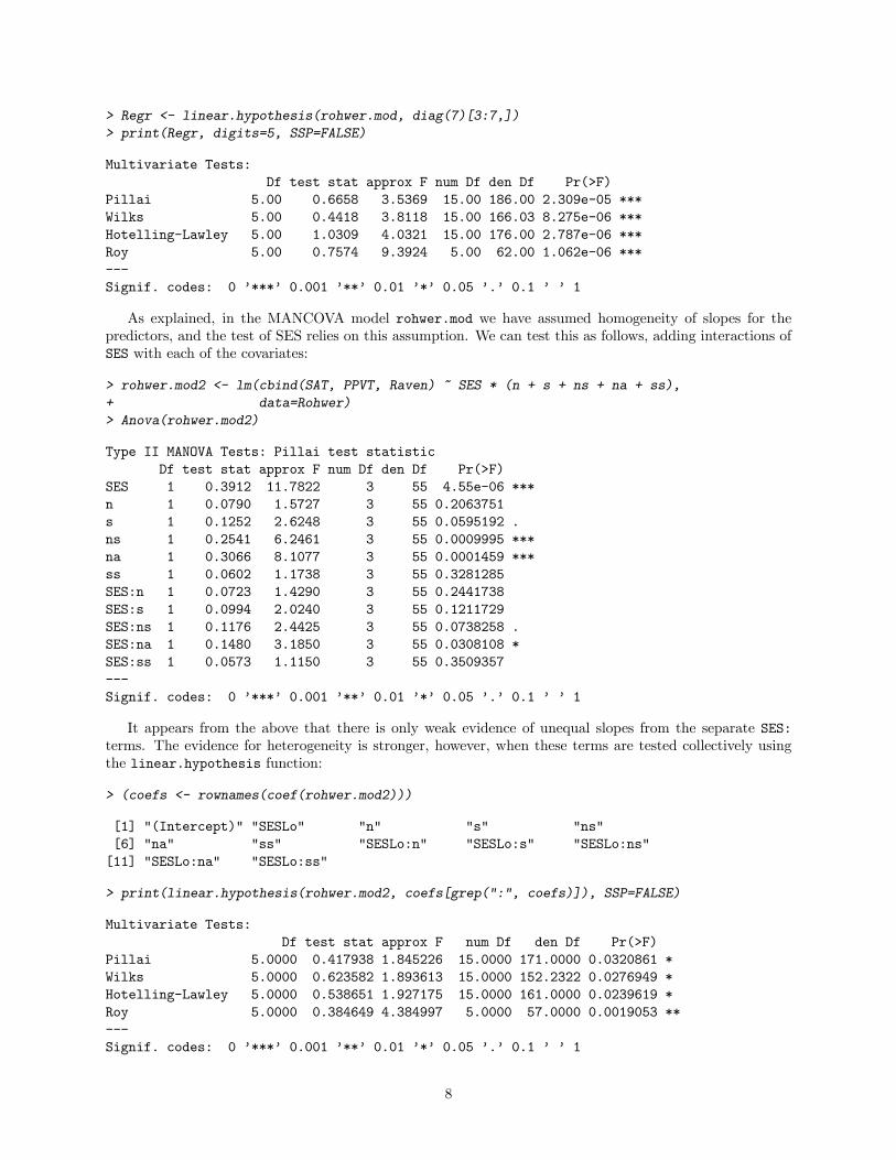
> Regr <- linear.hypothesis(rohwer.mod, diag(7)[3:7,])> print(Regr, digits=5, SSP=FALSE)

Multivariate Tests:Df test stat approx F num Df den Df Pr(>F)

Pillai 5.00 0.6658 3.5369 15.00 186.00 2.309e-05 ***Wilks 5.00 0.4418 3.8118 15.00 166.03 8.275e-06 ***Hotelling-Lawley 5.00 1.0309 4.0321 15.00 176.00 2.787e-06 ***Roy 5.00 0.7574 9.3924 5.00 62.00 1.062e-06 ***---Signif. codes: 0 ’***’ 0.001 ’**’ 0.01 ’*’ 0.05 ’.’ 0.1 ’ ’ 1

As explained, in the MANCOVA model rohwer.mod we have assumed homogeneity of slopes for thepredictors, and the test of SES relies on this assumption. We can test this as follows, adding interactions ofSES with each of the covariates:

> rohwer.mod2 <- lm(cbind(SAT, PPVT, Raven) ~ SES * (n + s + ns + na + ss),+ data=Rohwer)> Anova(rohwer.mod2)

Type II MANOVA Tests: Pillai test statisticDf test stat approx F num Df den Df Pr(>F)

SES 1 0.3912 11.7822 3 55 4.55e-06 ***n 1 0.0790 1.5727 3 55 0.2063751s 1 0.1252 2.6248 3 55 0.0595192 .ns 1 0.2541 6.2461 3 55 0.0009995 ***na 1 0.3066 8.1077 3 55 0.0001459 ***ss 1 0.0602 1.1738 3 55 0.3281285SES:n 1 0.0723 1.4290 3 55 0.2441738SES:s 1 0.0994 2.0240 3 55 0.1211729SES:ns 1 0.1176 2.4425 3 55 0.0738258 .SES:na 1 0.1480 3.1850 3 55 0.0308108 *SES:ss 1 0.0573 1.1150 3 55 0.3509357---Signif. codes: 0 ’***’ 0.001 ’**’ 0.01 ’*’ 0.05 ’.’ 0.1 ’ ’ 1

It appears from the above that there is only weak evidence of unequal slopes from the separate SES:terms. The evidence for heterogeneity is stronger, however, when these terms are tested collectively usingthe linear.hypothesis function:

> (coefs <- rownames(coef(rohwer.mod2)))

[1] "(Intercept)" "SESLo" "n" "s" "ns"[6] "na" "ss" "SESLo:n" "SESLo:s" "SESLo:ns"[11] "SESLo:na" "SESLo:ss"

> print(linear.hypothesis(rohwer.mod2, coefs[grep(":", coefs)]), SSP=FALSE)

Multivariate Tests:Df test stat approx F num Df den Df Pr(>F)

Pillai 5.0000 0.417938 1.845226 15.0000 171.0000 0.0320861 *Wilks 5.0000 0.623582 1.893613 15.0000 152.2322 0.0276949 *Hotelling-Lawley 5.0000 0.538651 1.927175 15.0000 161.0000 0.0239619 *Roy 5.0000 0.384649 4.384997 5.0000 57.0000 0.0019053 **---Signif. codes: 0 ’***’ 0.001 ’**’ 0.01 ’*’ 0.05 ’.’ 0.1 ’ ’ 1

8

4.4 Repeated-Measures MANOVA: O’Brien and Kaiser’s Data

O’Brien and Kaiser (1985: Table 7) describe an imaginary study in which 16 female and male subjects, whoare divided into three treatments, are measured on an unspecified response variable at a pretest, post-test,and a follow-up session; during each session, they are measured at five occasions at intervals of one hour.The design, therefore, has two between-subject and two within-subject factors. The data are in the dataframe OBrienKaiser in the car package:

> OBrienKaiser

treatment gender pre.1 pre.2 pre.3 pre.4 pre.5 post.1 post.2 post.3 post.4 post.51 control M 1 2 4 2 1 3 2 5 3 22 control M 4 4 5 3 4 2 2 3 5 33 control M 5 6 5 7 7 4 5 7 5 44 control F 5 4 7 5 4 2 2 3 5 35 control F 3 4 6 4 3 6 7 8 6 36 A M 7 8 7 9 9 9 9 10 8 97 A M 5 5 6 4 5 7 7 8 10 88 A F 2 3 5 3 2 2 4 8 6 59 A F 3 3 4 6 4 4 5 6 4 110 B M 4 4 5 3 4 6 7 6 8 811 B M 3 3 4 2 3 5 4 7 5 412 B M 6 7 8 6 3 9 10 11 9 613 B F 5 5 6 8 6 4 6 6 8 614 B F 2 2 3 1 2 5 6 7 5 215 B F 2 2 3 4 4 6 6 7 9 716 B F 4 5 7 5 4 7 7 8 6 7

fup.1 fup.2 fup.3 fup.4 fup.51 2 3 2 4 42 4 5 6 4 13 7 6 9 7 64 4 4 5 3 45 4 3 6 4 36 9 10 11 9 67 8 9 11 9 88 6 6 7 5 69 5 4 7 5 410 8 8 9 7 811 5 6 8 6 512 8 7 10 8 713 7 7 8 10 814 6 7 8 6 315 7 7 8 6 716 7 8 10 8 7

The contrasts specified for each between-subject factor correspond to what was employed in the originalsource:

> contrasts(OBrienKaiser$treatment)

[,1] [,2]control -2 0A 1 -1B 1 1

9

> contrasts(OBrienKaiser$gender)

[,1]F 1M -1

We fit a multivariate linear model to the O’Brien and Kaiser data, using

> mod.ok <- lm(cbind(pre.1, pre.2, pre.3, pre.4, pre.5,+ post.1, post.2, post.3, post.4, post.5,+ fup.1, fup.2, fup.3, fup.4, fup.5) ~ treatment*gender,+ data=OBrienKaiser)

As for the anova method for mlm objects, the factors defining the design on the response variables (the“intra-subject” or “within-subject” design) are given as a data frame via the idata argument to Anova.In contrast to anova, however, the intra-subject design itself is given to Anova as a model formula viathe idesign argument. This is a simpler approach but slightly less flexible: Anova requires that differentterms in the model matrix generated from idata and idesign are orthogonal to one another, although thecontrasts for each term need not be orthogonal: The model matrix for the intra-subject design is thereforeblock-orthogonal. This will be the case for the default contrast types that Anova employs for the intra-subjectdesign: contr.sum for factors and contr.poly for ordered factors. For the current example,

> phase <- factor(rep(c("pretest", "posttest", "followup"), c(5, 5, 5)),+ levels=c("pretest", "posttest", "followup"))> hour <- ordered(rep(1:5, 3))> idata <- data.frame(phase, hour)> idata

phase hour1 pretest 12 pretest 23 pretest 34 pretest 45 pretest 56 posttest 17 posttest 28 posttest 39 posttest 410 posttest 511 followup 112 followup 213 followup 314 followup 415 followup 5

The MANOVA employing this intra-subject data frame along with a crossed design on the intra-subjectfactors phase and hour is obtained as follows:

(av.ok <- Anova(mod.ok, idata=idata, idesign=~phase*hour, type="III"))

Type III Repeated Measures MANOVA Tests: Pillai test statisticDf test stat approx F num Df den Df Pr(>F)

(Intercept) 1 0.967 296.389 1 10 9.241e-09 ***treatment 2 0.441 3.940 2 10 0.0547069 .gender 1 0.268 3.659 1 10 0.0848003 .treatment:gender 2 0.364 2.855 2 10 0.1044692

10

phase 1 0.814 19.645 2 9 0.0005208 ***treatment:phase 2 0.696 2.670 4 20 0.0621085 .gender:phase 1 0.066 0.319 2 9 0.7349696treatment:gender:phase 2 0.311 0.919 4 20 0.4721498hour 1 0.933 24.315 4 7 0.0003345 ***treatment:hour 2 0.316 0.376 8 16 0.9183275gender:hour 1 0.339 0.898 4 7 0.5129764treatment:gender:hour 2 0.570 0.798 8 16 0.6131884phase:hour 1 0.560 0.478 8 3 0.8202673treatment:phase:hour 2 0.662 0.248 16 8 0.9915531gender:phase:hour 1 0.712 0.925 8 3 0.5894907treatment:gender:phase:hour 2 0.793 0.328 16 8 0.9723693---Signif. codes: 0 ’***’ 0.001 ’**’ 0.01 ’*’ 0.05 ’.’ 0.1 ’ ’ 1

The Type-III tests correspond to the example presented in O’Brien and Kaiser (1985), and depend uponusing contrasts for the between-subject factors that are orthogonal in the row-basis of the model matrix, asis the case for the contrasts (contr.sum and contr.poly) employed in the example.The summary method for Anova.mlm is also capable of computing the traditional mixed-model F tests

for repeated measures under the assumption of compound symmetry: that is, that the covariance matrixof the responses has equal diagonal elements (variances) and equal off-diagonal elements (covariances –implying constant correlation between measures). The output includes traditional Greenhouse-Geiser andHuynh-Feldt corrections for departures from compound symmetry:

summary(av.ok, multivariate=FALSE)

Univariate Type III Repeated-Measures ANOVA Assuming Compound Symmetry

SS num Df Error SS den Df F Pr(>F)(Intercept) 6759.3 1 228.1 10 296.3888 9.241e-09 ***treatment 179.7 2 228.1 10 3.9405 0.054707 .gender 83.4 1 228.1 10 3.6591 0.084800 .treatment:gender 130.2 2 228.1 10 2.8555 0.104469phase 129.5 2 80.3 20 16.1329 6.732e-05 ***treatment:phase 77.9 4 80.3 20 4.8510 0.006723 **gender:phase 2.3 2 80.3 20 0.2828 0.756647treatment:gender:phase 10.2 4 80.3 20 0.6366 0.642369hour 104.3 4 62.5 40 16.6857 4.027e-08 ***treatment:hour 1.2 8 62.5 40 0.0933 0.999245gender:hour 2.8 4 62.5 40 0.4503 0.771559treatment:gender:hour 7.8 8 62.5 40 0.6204 0.755484phase:hour 11.3 8 96.2 80 1.1799 0.321587treatment:phase:hour 6.6 16 96.2 80 0.3453 0.990125gender:phase:hour 9.0 8 96.2 80 0.9313 0.495612treatment:gender:phase:hour 14.2 16 96.2 80 0.7359 0.749562---Signif. codes: 0 ’***’ 0.001 ’**’ 0.01 ’*’ 0.05 ’.’ 0.1 ’ ’ 1

Greenhouse-Geisser and Huynh-Feldt Correctionsfor Departure from Compound Symmetry

GG eps Pr(>F[GG])phase 0.79953 0.0002814 ***treatment:phase 0.79953 0.0126909 *

11

gender:phase 0.79953 0.7089599treatment:gender:phase 0.79953 0.6116209hour 0.46028 9.763e-05 ***treatment:hour 0.46028 0.9786227gender:hour 0.46028 0.6284344treatment:gender:hour 0.46028 0.6413625phase:hour 0.44950 0.3345212treatment:phase:hour 0.44950 0.9303725gender:phase:hour 0.44950 0.4490777treatment:gender:phase:hour 0.44950 0.6463449---Signif. codes: 0 ’***’ 0.001 ’**’ 0.01 ’*’ 0.05 ’.’ 0.1 ’ ’ 1

HF eps Pr(>F[HF])phase 0.92786 0.0001125 ***treatment:phase 0.92786 0.0084388 **gender:phase 0.92786 0.7408568treatment:gender:phase 0.92786 0.6319975hour 0.55928 2.301e-05 ***treatment:hour 0.55928 0.9886617gender:hour 0.55928 0.6645541treatment:gender:hour 0.55928 0.6692976phase:hour 0.73306 0.3296590treatment:phase:hour 0.73306 0.9752254gender:phase:hour 0.73306 0.4780341treatment:gender:phase:hour 0.73306 0.7080122---Signif. codes: 0 ’***’ 0.001 ’**’ 0.01 ’*’ 0.05 ’.’ 0.1 ’ ’ 1

5 Hypothesis-Error (HE) PlotsHypothesis-error (or HE) plots use ellipses to represent hypothesis and error sums of squares and productmatrices. The plots are implemented in two and three dimensions in the heplots package for R.The error ellipse is obtained by dividing the SSPE by the error degrees of freedom n − p, producing a

data ellipse for the residuals. The SSPE ellipse is also centered at the grand means, allowing individualfactor means to be shown on the same plot, facilitating interpretation.We consider two scalings of the hypothesis ellipse:

1. “Evidence-based” scaling, the default, in which the hypothesis ellipse protrudes from the error ellipseif and only if the hypothesis can be rejected by the Roy maximum-root criterion. The directionsin which the hypothesis ellipse exceed the error ellipse are informative about the responses or theirlinear combinations that depart significantly from H0. This scaling is produced by dividing SSPH byλα(n− p) , where λα is the critical value of Roy’s statistic for a test at level α.

2. Scaling by “effect size,” where the hypothesis ellipse is put on the same scale as the error ellipse, andapproximately represents the data ellipse of fitted values under the alternative hypothesis. Here, SSPH

is simply divided by n− p.

All of this extends straightforwardly to the three dimensional case.

5.1 HE Plots for the Pottery Data

The Romano-British pottery data were described in Section 4.1. Recall that there are four response variablesrepresenting the chemical content of aluminium, iron, magnesium, calcium, and sodium in 26 samples of

12

10 12 14 16 18 20

02

46

8

Al

Fe +

Error

Site

AshleyRails

Caldicot

IsleThorns

Llanedyrn

Caldicot & Isle ThornsC-A

I-A

C-A

I-A

C-A

I-A

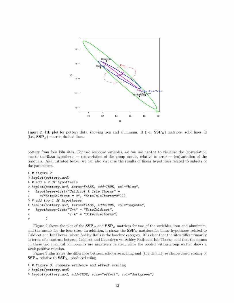
Figure 2: HE plot for pottery data, showing iron and aluminum. H (i.e., SSPH) matrices: solid lines; E(i.e., SSPE) matrix, dashed lines.

pottery from four kiln sites. For two response variables, we can use heplot to visualize the (co)variationdue to the Site hypothesis – (co)variation of the group means, relative to error – (co)variation of theresiduals. As illustrated below, we can also visualize the results of linear hypotheses related to subsets ofthe parameters.

> # Figure 2> heplot(pottery.mod)> # add a 2 df hypothesis> heplot(pottery.mod, terms=FALSE, add=TRUE, col="blue",+ hypotheses=list("Caldicot & Isle Thorns" =+ c("SiteCaldicot = 0", "SiteIsleThorns=0")))> # add two 1 df hypotheses> heplot(pottery.mod, terms=FALSE, add=TRUE, col="magenta",+ hypotheses=list("C-A" = "SiteCaldicot",+ "I-A" = "SiteIsleThorns")+ )

Figure 2 shows the plot of the SSPH and SSPE matrices for two of the variables, iron and aluminum,and the means for the four sites. In addition, it shows the SSPH matrices for linear hypotheses related toCaldicot and IsleThorns, where Ashley Rails is the baseline category. It is clear that the sites differ primarilyin terms of a contrast between Caldicot and Llanedryn vs. Ashley Rails and Isle Thorns, and that the meanson these two chemical components are negatively related, while the pooled within group scatter shows aweak positive relation.Figure 3 illustrates the difference between effect-size scaling and (the default) evidence-based scaling of

SSPH relative to SSPE , produced using

> # Figure 3: compare evidence and effect scaling> heplot(pottery.mod)> heplot(pottery.mod, add=TRUE, size="effect", col="darkgreen")

13

10 12 14 16 18 20

02

46

8

Al

Fe +

Error

Site

AshleyRails

Caldicot

IsleThorns

Llanedyrn

Site

Figure 3: HE plot for pottery data: Effect scaling (dark green) vs. evidence scaling (light green).

The evidence-scaled hypothesis ellipse for this one-way MANOVA model is the data ellipse for the groupmeans weighted by group sample sizes.Of course, other pairs of response variables can also be displayed (e.g., heplot(pottery.mod, variables=c("Mg",

"Fe")), or subsets of three response variables can be examined (by heplot3d(pottery.mod, variables=c(...)– see below). Alternatively, the variation across sites on all chemical components may be seen in the pair-wise 2D projections of the HE plot matrix in Figure 4. This graph was produced by the pairs method formlm objects, reordering the variables to produce a more coherent display (Friendly and Kwan, 2003):

> # Figure 4> pairs(pottery.mod, variables=c("Mg","Fe","Ca","Na","Al"))

Quite a lot may be read directly from this plot. For example: the site means for magnesium (Mg) andiron (Fe) are nearly perfectly correlated, and have the same pattern with all other variables, while all meandifferences for aluminium (Al) are in the opposite direction. The relations for calcium (Ca) and sodium (Na)also differ somewhat from those for magnesium and iron in that Caldicot samples are quite high on calcium,while Llanedryn is high on sodium.

5.2 HE Plots for the Plastic Data

HE plots are particularly instructive when there are multiple sources of hypothesis variation to be tested in amultivariate linear model. The simplest case is for a 2×2 MANOVA, where the main effects and interactioneach have 1 df (and so, the SSPH ellipsoids collapse to lines), but where the response variable space is 2 ormore dimensional. The plastic-film data were introduced in Section 4.2. There are, recall, two dichotomousfactors (rate of extrusion and amount of an additive) and three response variables (tear resistance, film gloss,and opacity).In Figure 5, we show the HE plot for the first two response variables (tear and gloss). In this plot, we

overlay the size="evidence" and size="effect" scalings, varying line width. Note that, in this view, theeffect for additive does not extend outside the error ellipse.

14

Mg

10.1

20.8

+Error

Site

AshleyRails

Caldicot

IsleThorns

Llanedyrn

+Error

Site

AshleyRails

Caldicot

IsleThorns

Llanedyrn

+Error

Site

AshleyRails

Caldicot

IsleThorns

Llanedyrn

+Error

Site

AshleyRails

Caldicot

IsleThorns

Llanedyrn

+Error

Site

AshleyRails

Caldicot

IsleThorns

Llanedyrn

Fe

0.92

7.09

+Error

Site

AshleyRails

Caldicot

IsleThorns

Llanedyrn

+Error

Site

AshleyRails

Caldicot

IsleThorns

Llanedyrn

+Error

Site

AshleyRails

Caldicot

IsleThorns

Llanedyrn

+

Error

Site

AshleyRails

Caldicot

IsleThorns

Llanedyrn

+Error

Site

AshleyRails

Caldicot

IsleThorns

Llanedyrn

Ca

0.53

7.23

+

Error

Site

AshleyRails

Caldicot

IsleThorns

Llanedyrn

+

Error

Site

AshleyRails

Caldicot

IsleThorns

Llanedyrn

+

ErrorSite

AshleyRailsCaldicotIsleThorns

Llanedyrn

+

ErrorSite

AshleyRailsCaldicotIsleThorns

Llanedyrn

+

ErrorSite

AshleyRails CaldicotIsleThorns

Llanedyrn

Na

0.01

0.31

+

Error

Site

AshleyRailsCaldicot IsleThorns

Llanedyrn

+

ErrorAshleyRails

Caldicot

IsleThorns

Llanedyrn+

ErrorAshleyRails

Caldicot

IsleThorns

Llanedyrn+

ErrorAshleyRails

Caldicot

IsleThorns

Llanedyrn+

ErrorAshleyRails

Caldicot

IsleThorns

LlanedyrnAl

0.03

0.54

Figure 4: pairs HE plot matrix for the pottery data.

15

6.2 6.4 6.6 6.8 7.0 7.2 7.4

8.8

9.0

9.2

9.4

9.6

9.8

tear

glos

s

+

Error

rate

additiverate:additiveLow

HighLow

High

Figure 5: HE plot for tear and gloss in the Plastic data. Thick lines: evidence scaling; thin lines: effectscaling.

> # Figure 5: Compare evidence and effect scaling> heplot(plastic.mod, size="evidence")> heplot(plastic.mod, size="effect", add=TRUE, lwd=8, term.labels=FALSE)

In addition to linear hypotheses that decompose multiple-df tests into their constituents (as in Figure2), we can also compose linear hypotheses by summing effects. Figure 6, for example adds SSPH ellipsescorresponding to the sum of main effects (additive+rate) and for the variation of all four groups, as if ina one-way design.

> # Figure 6: Ellipses for composite effects:> # Group=rate*additive and Main=rate+additive> heplot(plastic.mod, hypotheses=list("Group" =+ c("rateHigh", "additiveHigh", "rateHigh:additiveHigh")))> heplot(plastic.mod, hypotheses=list("Main" =+ c("rateHigh", "additiveHigh")), terms=FALSE,+ add=TRUE, col="orange")

Again, we can see the (co)variation due to hypothesis and error for all response variables in the pairsplot (see Figure 7). Note that the effect of additive, while significant in the multivariate test does not quiteprotrude beyond the SSPE ellipse in any of these 2D projections.

> # Figure 7> pairs(plastic.mod)

Using heplot3d, we can easily find 3D views of all effects that show the significant effects of bothadditive and rate, as shown in Figure 8.

> # Figure 8> heplot3d(plastic.mod)

16

6.0 6.5 7.0 7.5

8.5

9.0

9.5

10.0

tear

glos

s

+

Error

rate

additiverate:additive

Group

Low

HighLow

High

Main

Figure 6: HE plot for tear and gloss, showing the SSPH matrices for the summed Main effects and for allGroups.

5.3 HE Plots for the Rohwer Data

The ideas behind HE plots extend naturally to multivariate multiple regression and multivariate analysis ofcovariance. To illustrate, we turn to the Rohwer data, introduced in Section 4.3.A 2D view of the additive MANCOVA model that we fit to the Rohwer data and the overall test for all

covariates is provided in Figure 9, produced using heplot as follows:

> # Figure 9> colors <- c("red", "blue", rep("black",5), "darkgrey")> heplot(rohwer.mod, col=colors,+ hypotheses=list("Regr" = c("n", "s", "ns", "na", "ss"))+ )

This display immediately extends to all 2D views using pairs (Figure 10) and to a 3D plot using heplot3d(Figure 11). It may be seen that the predicted values for all three responses are positively correlated, andthat the hypothesized effects of the covariates span the full three dimensions of the responses. As well, theHigh SES group is higher on all responses than the Low SES group.

> # Figures 10 and 11> pairs(rohwer.mod, col=colors,+ hypotheses=list("Regr" = c("n", "s", "ns", "na", "ss")))> heplot3d(rohwer.mod, col=colors,+ hypotheses=list("Regr" = c("n", "s", "ns", "na", "ss")))

In Section 4.3, we also fit a model to the Rohwer data relaxing the assumption of equal slopes – that is,permitting interactions between the covariates and SES. There are several options for visualization: Eitherwe can fit and display separate models for the High and Low SES groups (which also allows the within-groupserror-covariance matrices to differ); we can fit a combined model with separate intercept and slopes for thetwo groups, which assumes a common within-groups error-covariance matrix; or we can try to visualize theslope differences in the heterogeneous-slopes model rohwer.mod2. Choosing the last option, we examine theHE pairs plot in Figure 12. To simplify this display, we show the hypothesis ellipses for the overall effectsof the PA tests in the baseline high-SES group, and a single combined ellipse for all the SESLo: interaction

17

tear

5.8

7.6

+

Error

rate

additive

rate:additive

Low

High

Low

High

+

Error

rate

additive

rate:additive

Low

High

Low

High

+

Error

rate

additiverate:additiveLow

HighLow

High

gloss

8.3

10.1

+

Errorrate

additiverate:additiveLow

HighLow

High

+

Error

rate

additiverate:additive

LowHigh

Low

High

+

Error

rate

additiverate:additive

LowHigh

Low

High

opacity

0.8

8.4

Figure 7: HE pairs plot for the Plastic data.

18

Figure 8: heplot3d plot for the Plastic data.

19

0 20 40 60 80

4050

6070

8090

100

SAT

PP

VT

+

Error

SES

n

s

ns

na

ss

Regr

Hi

Lo

Figure 9: HE plot for SAT and PPVT in the Rohwer data. The ellipse labeled Regr shows the combined effectof the covariates.

terms that we tested previously, representing differences in slopes between the low and high-SES groups.Because SES is “treatment-coded” in this model, the ellipse for each covariate represents the hypothesis thatthe slopes for that covariate are zero in the high-SES baseline category.

> # Figure 12> pairs(rohwer.mod2, col=c(colors, "brown"),+ terms=c("SES", "n", "s", "ns", "na", "ss"),+ hypotheses=list("Regr" = c("n", "s", "ns", "na", "ss"),+ "Slopes" = coefs[grep(":", coefs)]))

Comparing Figures 10 and 12 for the homogeneous and heterogenous-slopes models, it may be seen thatmost of the covariates have ellipses of similar size and orientation, reflecting similar evidence against thenull hypotheses in the baseline high-SES group and for both groups in the common-slopes model; so toodoes the effect of SES, with the High SES group performing better on all measures. The error covariation isnoticeably smaller in some of the panels of Figure 12 (those for SAT and PPVT), reflecting additional variationaccounted for by differences in slopes.

ReferencesDempster, A. P. (1969). Elements of Continuous Multivariate Analysis. Addison-Wesley, Reading MA.

Fox, J. (2002). An R and S-PLUS Companion to Applied Regression. Sage, Thousand Oaks CA.

Friendly, M. (2006). Data ellipses, HE plots and reduced-rank displays for multivariate linar models: SASsoftware and examples. Journal of Statistical Software, 17(6):1—42.

Friendly, M. (2007). HE plots for multivariate general linear models. Journal of Computational and GraphicalStatistics, 17:in press.

Friendly, M. and Kwan, E. (2003). Effect ordering for data displays. Computational Statistics and DataAnalysis, 43:509—539.

20

SAT

1

99

+

Error

SESn

s

nsna

ss

Regr

Hi

Lo +

Error

SESn

s

nsna

ss

Regr

Hi

Lo

+

Error

SES

n

s

ns

na

ss

Regr

Hi

LoPPVT

40

105

+

Error

SES

n

sns

na

ss

Regr

Hi

Lo

+

Error

SES

n

s

ns

nass

Regr

Hi

Lo +

Error

SES

n

s

ns

nass

Regr

Hi

Lo Raven

8

21

Figure 10: HE pairs plot for the Rohwer data.

21

Figure 11: heplot3d plot for the Rohwer data.

22

SAT

1

99

+

Error

SESn

s

ns na

ss

Regr

Slopes

Hi

Lo +

Error

SESn

s

ns

na

ss

Regr

Slopes

Hi

Lo

+

Error

SES

n

s

ns

na

ss

Regr

SlopesHi

LoPPVT

40

105

+

Error

SES

n

sns

na

ss

Regr

SlopesHi

Lo

+

Error

SES

n

s

ns

na

ss

RegrSlopes

Hi

Lo +

Error

SES

n

s

ns

na

ss

RegrSlopes

Hi

Lo Raven

8

21

Figure 12: pairs plot for heterogeneous regression model rohwer.mod2. The ellipses labeled “Slopes” showthe covariation of all terms for slope differences between the High and Low SES groups.

23

Hand, D., Daly, F., Lunn, A. D., McConway, K. J., and Ostrowski, E. (1994). A Handbook of Small DataSets. Chapman and Hall, London.

Johnson, R. A. and Wichern, D. W. (1992). Applied Multivariate Statistical Analysis. Prentice Hall, Engle-wood Cliffs NJ, third edition.

Monette, G. (1990). Geometry of multiple regression and interactive 3-D graphics. In Fox, J. and Long,J. S., editors, Modern Methods of Data Analysis, pages 209—256. Sage, Beverly Hills CA.

O’Brien, R. G. and Kaiser, M. K. (1985). MANOVA method for analyzing repeated measures designs: Anextensive primer. Psychological Bulletin, 97:316—333.

Timm, N. H. (1975). Multivariate Analysis with Applications in Education and Psychology. Wadsworth(Brooks/Cole), Belmont CA.

Tubb, A., Parker, A., and Nickless, G. (1980). The analysis of Romano-British pottery by atomoic absorbtionspectrophotometry. Archaeometry, 22:153—171.

24