Visioning Vs. Modeling: Analyzing the Land Use-Transportation

Futures of Urban Regions

By

Jason D. Lemp

Graduate Student Researcher

The University of Texas at Austin

6.508. Cockrell Jr. Hall

Austin, TX 78712-1076

jdl880@mail.utexas.edu

Bin (Brenda) Zhou

Graduate Student Researcher

The University of Texas at Austin

6.508. Cockrell Jr. Hall

Austin, TX 78712-1076

brendazhou@mail.utexas.edu

Kara M. Kockelman

(Corresponding author)

Associate Professor and William J. Murray Jr. Fellow Department

of Civil, Architectural and Environmental Engineering The

University of Texas at Austin

6.9 E. Cockrell Jr. Hall

Austin, TX 78712-1076

kkockelm@mail.utexas.edu

Phone: 512-471-0210

FAX: 512-475-8744

Barbara M. Parmenter

Assistant Professor

Community and Regional Planning Program

The University of Texas at Austin

1 University Station B7500

Austin, Texas 78712

The University of Texas at Austin

3.124B Sutton Hall Austin,

TX 78712-1076

bparmenter@mail.utexas.edu

The following paper is a pre-print and the final publication can be found in

Journal of Urban Planning and Development, 134 (3):97-109, 2008.

Presented at the 86th Annual Meeting of the Transportation Research Board,

January 2007

2

Abstract In recent years, the use of visioning as a tool for developing regional land use scenarios has become rather common. Typically, visioning is performed in a cooperative of business owners, the community, and local officials, and results in a set of regional development goals for the region’s future. This is a very different approach to thinking about a region’s future than predictive models calibrated on historical data. In general, visions are created on the basis of stakeholder preferences. Consequently, direct comparisons of results for the two methods are not really relevant. However, it is important to understand how the two approaches differ and that both offer their own relative advantages from a planning perspective. In an effort to better appreciate what each approach offers, this paper compares and contrasts these two methods, featuring the Austin Metropolitan Statistical Area (MSA) as a case study. The preferred vision, produced by the Envision Central Texas (ECT) organization, offers the greatest potential for public involvement in identifying regional development goals for the future. The land use models have a strong theoretical foundation and allows for interactions with a transportation model. Moreover, the land use models have the potential to identify key strategies that can be used in achieving the region’s goals. Thus, the combination of these two approaches seems to offer the greatest opportunities for planners to achieve a future that accommodates all stakeholders. Key Words: visioning, land use models, urban land use-transportation futures

3

INTRODUCTION For several decades, planners have recognized the need to prepare for future community needs and challenges, resulting in a variety of travel demand and land use modeling approaches. The outputs of land use models are important inputs to transportation models, as well as air quality models (where on-road emissions are just one source of pollutants and their precursors). Land use models allow one to forecast the location and intensity of non-mobile sources, including biogenic emissions. Thanks to increasing computational power and GIS-capabilities, land use and transportation models (e.g., Clarke’s SLEUTH, De la Barra’s TRANUS, Waddell’s UrbanSim, MORPC’s Activity-Based TDM, Bhat’s CEMDAP) have become more elaborate. Nevertheless, a region’s land use future remains an uncertain one. The number of factors that influence whether development occurs and to what extent is enormous. Moreover, past trends are not necessarily the direction communities wish to head. Consequently, scenario planning has grown in use recently, particularly that which is referred to as visioning (Bartholomew 2005). Visioning is a highly community oriented planning technique used to create regional land use and transportation goals (FHWA 1996). Unlike modeling, it is not a means of prediction. Instead, it offers stakeholders an opportunity to provide input (via for example, public meetings and community surveys) about development features most important to them, ideally allowing them to imagine and create a regional future that accommodates all stakeholders’ interests (FHWA 1996). Such projects develop strategies to reach the final vision, and are undertaken with a 20- to 30-year horizon in mind, consistent with typical land use and transportation modeling endeavors. While the focus is generally on land use patterns, traffic prediction often occurs at the end of the process, as a point of comparison, using standard travel demand models (e.g., BRTB 2003, ECT 2004, SCAG 2004, TCRPC 2005). In contrast to visioning, land use models are based on historical trends and attempt to forecast or predict what future land use will look like based on those historic trends. They rely profoundly on data and model specification, rather than community opinion and aspirations. The data used to estimate such mathematical models includes land use inventories, zoning policies, highway networks, and employment and households by zone. If traffic estimates are desired, both methods turn to travel demand models. The predictions of these land use and travel demand models are assumed to reflect the underlying behaviors and preferences that the study area’s residents, employers, and land developers have exhibited in the past (subject to in-migration, changing demographics, exogenous shocks, etc.). The better land use models are sensitive to changes in policies like zoning, as well as to travel costs (via for example, congestion, construction of new highways, imposition of roadway tolls, and expansion of transit services). The travel demand models are sensitive to household location and composition, interzonal travel costs, zonal attraction levels, and so on. The outputs of these mathematical models are effectively an extension of historical trends under implementation of certain policies, subject to each model specification’s intrinsic limitations (such as spatial and demographic aggregation of households, as well as neglect of key variables [like soil type, school quality, and vehicle purchase costs]). They are not community visions

4

created by a variety of stakeholders. Instead, they typically are tightly controlled by a few analysts, either in-house (at a metropolitan planning organization, for example) or hired as consultants. Nevertheless, both the modeling and visioning approaches tend to rely on mathematical models for their traffic estimates. Thus, their key difference lies in generating the land use forecasts/visions. In addition to these two distinct techniques of analyzing future land use, Delphi techniques provide another way to predict future land uses under alternative plans (e.g. see Ervin 1977, Cavalli-Sforza and Ortolano 1983, Wisconsin Department of Transportation 1993). Delphi method is a technique in which opinions of a Delphi panel that have both past experience and in-depth knowledge regarding the events under study are obtained. Consistent predictions and satisfactory agreement among panelists are reached in an iterative fashion. It is believed that the forecasts obtained from a Delphi panel are more likely to be realistic and firmly grounded compared to the forecasts from laypersons; however, this method involves a large amount of information in the long and complex Delphi questionnaires that requires substantial time from both the analysts and the panelists (Cavalli-Sforza and Ortolano 1983). EXISTING VISIONS Nearly all visioning projects begin and end with intensive public involvement. The role the community plays in creating a vision for a particular region arguably is the most important component of visioning. The Baltimore Vision 2030 effort conducted focus groups, stakeholder interviews, regional workshops, and phone surveys in developing a preferred future vision of the region (BRTB 2003). Throughout the process, residents were asked for their opinions and perceptions on various topics. Similarly, the leaders of Phoenix’s Valley Vision 2025 (MAG 2000) and Envision Utah (Envision Utah 2003) emphasized community involvement by conducting interviews and holding workshops, meetings, and committees throughout the process. With the introduction of the 1969 National Environmental Policy Act (NEPA) (42 U.S.C. § 4332) and the1991 Intermodal Surface Transportation Efficiency Act (ISTEA), the importance of informing the community on planning issues has become widely accepted. Visioning projects around the nation have all taken proactive roles in getting residents involved in the process, while cultivating regional support. A second feature in many visioning projects is the development of a set of guiding principles or values for the region (e.g., CRT 2003, SCAG 2004, SANDAG 2004, TCRPC 2005, SACOG 2005). These are based primarily on public input gained during the outreach initiatives discussed above, and tend to be very general. They range from mobility, sustainability, prosperity, and livability in the Los Angeles’ Southern California Compass visioning project (SCAG 2004), to urban form, transportation, housing, environment, economic prosperity, and public facilities in San Diego’s Regional Comprehensive Plan (SANDAG 2004). In the case of the Southern California Compass, guiding principles were intended to organize strategies for future development and provide guidance for future growth decisions (SCAG 2004). All regional visioning projects involve the development of one or multiple visions of the region’s future. In most cases this takes the form of particular scenarios (e.g., PSRC 1995, MAG 2000, BAASC 2002, CRT 2003, BRTB 2003, Envision Utah 2003, ECT 2004, TCRPC 2005). In

5

general, the community participation process is used to create a set of alternative scenarios. Phoenix’s Valley Vision 2025 process resulted in the development of four distinct scenarios. These included a base case or “do nothing different” scenario, an urban revitalization scenario with significant infill development, a scenario development focused in city centers, and a fringe growth scenario (MAG 2003). The TCRPC developed just two scenarios for comparison, a base scenario and a “wise growth” scenario (TCRPC 2005). In some cases, a single alternative is chosen as the “preferred” growth scenario (Envision Utah, 2003, TCRPC 2005). However, in other cases, community input helps to identify the most preferable (based on community opinions) characteristics from each alternative, which forms the basis for the creation of a final “preferred” regional scenario (BAASC 2002, CRT 2003, ECT 2004). The final two stages of visioning are strategy development and implementation. Strategies tend to be somewhat broad, but are similar across regions with similar goals. In contrast, implementation varies more across regions, and depends greatly on the power and status the visioning organization enjoys in the region, on the state’s land use regulatory framework, and on the regional jurisdictional context. Ultimately, a vision will have one of three fates in the context of regional planning: 1) it is fully incorporated (e.g., Smart Growth Strategy/Regional Livability Footprint in Bay Area, Southern California Compass in Los Angeles, and Vision 2020 in Seattle), 2) it is partially incorporated (e.g., Regional Transportation Plan in Phoenix), or 3) it is ignored (e.g., Vision 2020 in San Diego and Vision 2030 in Baltimore) (Bartholomew ND). Particular details differ from one vision to another to make the vision relevant to a region. Every region faces its own specific features that require unique consideration. While Envision Central Texas (ECT) shares many common attributes with the visions described in this section, there exist important differences that are described as a case study in later sections. LAND USE MODELS Due to land use’s significant environmental impacts, both environmental and transportation legislation (including, e.g., the 1990 Clean Air Act Amendments, ISTEA [in 1991], TEA-21 [in 1998], and SAFETEA-LU [in 2005]) require modeling of travel and emissions with consistent land use patterns. Thus, the legislation directly and indirectly encourages the development and application of a variety of land use models. Concurrently, many studies summarized and compared the available land use models. For example, Rosenbaum and Koenig (1997) evaluated 3 land use models on their ability to estimate the impacts of land use policies and strategies. NCHRP Report 423A (1999) described 8 leading land use models with a focus on assessing the impacts of transportation projects. Miller et al. (1998) addressed the issues in developing “ideal” land use models after detailed discussion on 6 integrated land use models. The U.S. Environmental Protection Agency (EPA) (2000) compared 22 land-uses change models to facilitate effective planning decision-making. The common consent is that no model is ideal and the most appropriate land use model varies with different situations. Some land use models emphasize scenario analysis, such as Klosterman’s What if? (Klosterman 1999, 2001, Pettit 2005) and Johnston’s UPLAN (Johnston and Shabazian 2003). In What if?, users control the suitability of land supply for different uses by specifying importance weights, suitability ratings and land use convertibility levels; in UPLAN, they specify attractiveness

6

criteria, which characterize land value and accessibility. The models then allocate demand for each land use type in order of suitability/attractiveness. These models are similar to the visioning process in the sense that users largely control the outputs. In addition, they lack a strong theoretical foundation, statistical roots, feedbacks, and rigorous mathematics. They simply place demand at the sites felt to be most attractive for development. However, they are easy to implement, if one has a detailed land inventory and a strong sense of demand. Most available mathematical models of land use fall into one of four major categories: Lowry’s gravity model, cellular automata, input-output, and discrete response simulation models. In gravity models, regional accessibility is core to the spatial allocation of jobs and households. Other factors that represent non-accessibility in nature, such as price adjustment and topographic conditions, are overlooked. A representative gravity model is the FHWA-sponsored Transportation Economic and Land Use Model (TELUM). This free software was built based on Putman’s Integrated Transportation and Land Use Package (ITLUP), and thus includes a Disaggregate Residential Allocation Model (DRAM), an Employment Allocation Model (EMPAL), and a standard travel demand model (e.g., see Watterson 1990 and Putman 1995). With total regional population and employment by economic sector and other specifications, TELUM uses current and historical residential and employment data to predict future conditions by household classes and employment sectors. Allocation is done at the zonal level, and TELUM does not perform well with disaggregate zonal systems or sparse zonal activity (NCHRP Report 423A, 1999). Cellular automata (CA) models represent a dynamic system in which discrete cellular states are updated according to a cell’s own state, as well as that of its neighbors. CA approaches are useful for representing relationships between a location and its immediate environment, permitting rapid simulation of large-scale cell-based systems. Clarke’s SLEUTH model (of Slope, Land use, Exclusion, Urban extent, Transportation and Hill shade) has been applied to several urban areas, in the U.S. and abroad (Clarke et al. 1997, Clarke and Gaydos 1998, Silva and Clarke 2002, Syphard et al. 2005). It relies on just five coefficients for four types of growth (termed spontaneous, spreading, edge, and road-influenced). These parameters tend to be calibrated in a rather ad hoc fashion, by minimizing a variety of discrepancy measures, using historical data to kick off the system and current data for comparison. Presently, CA models and their estimation lack economic and statistical foundations. Input-output models model the spatial and economic interactions of employment and household sectors across zones. They apply discrete choice models for mode and input choices, in order to meet exogenous demand for production. Representative models include De la Barra’s TRANUS (de la Barra 1989, Johnston and De la Barra 2000), Echenique’s MEPLAN (Abraham and Hunt 1999a, 1999b), and Kockelman’s RUBMRIO (Zhao and Kockelman 2004, Kockelman et al. 2004, Ruiz-Juri and Kockelman 2006). In these models, travel demand is a function of travel cost, and equilibrium between demand and supply for land is reached via implicit price adjustments. TRANUS also incorporates terminal and shipping costs and generates indicators to evaluate scenarios, from social, economic, financial and energy perspectives. However, the input-output framework is focused on trade, and most suitable for state-level or large metropolitan areas. Application at a small spatial scale is questionable, not to mention at the level of parcels and/or individual decision makers.

7

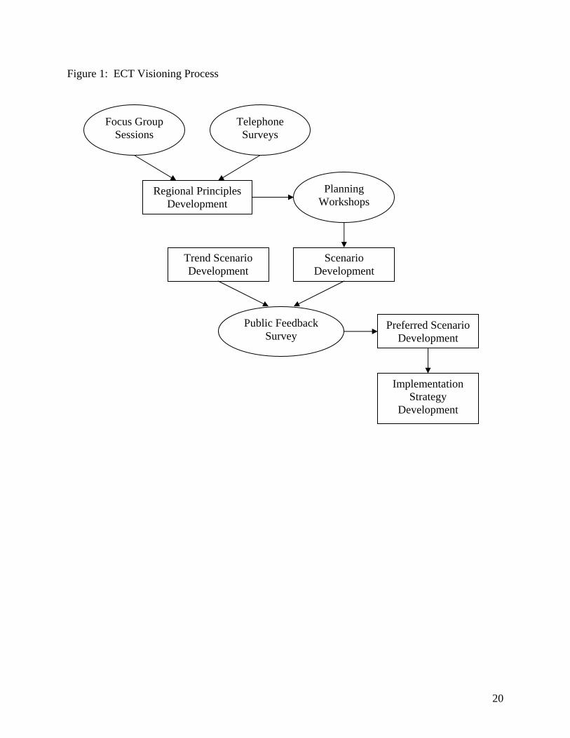
Random utility maximization and discrete choice theory (McFadden 1978) is the basis for the logit models found in Landis’ California Urban Futures models (CUF I [Landis 1994, 1995] and CUF II [Landis and Zhang 1998a, 1998b])1. The first of these allocates new development according to real estate profitability, while the second is more general, incorporating more land use types via a series of probabilistic equations. Adding further behavioral mechanisms, Waddell’s UrbanSim (Waddell 2002, Waddell et al. 2003, Waddell and Ulfarsson 2004) seeks to simulate the land-market interactions (and location choices) of households, firms, developers, and public actors. UrbanSim is highly disaggregate in terms of space, time, and agents, and is dynamic with constrained lags in household and business response to changes in supply of land and built space. In addition, UrbanSim is open source, and can be expanded by users. Nevertheless, a major limitation of these choice-based models is their intense data requirements (e.g., EPA 2000). The following sections describe the Austin case study in question here, and introduce the disaggregate, discrete- and continuous-response models used at the parcel and zonal levels to tackle one of region’s most complex questions: What does the future hold for its land use (and traffic) patterns? A CASE STUDY OF AUSTIN, TEXAS The Central Texas region consists of five counties: Bastrop, Caldwell, Hays, Travis, and Williamson. The region includes Austin, the state capital, and is populated by over 1.25 million people. This population is expected to double in the next 20 to 40 years. The Envision Central Texas (ECT) organization was founded in 2002 by concerned community leaders. Similar to other visioning projects, the organization’s mission is “to assist in the public development and implementation of a regional vision addressing the growth of Central Texas” to “preserve and enhance [the] region’s quality of life, natural resources, and economic prosperity” (ECT 2003d). As with other regional visions, the organization solicited input from the entire community to create a unified regional vision (ECT 2003d, 2004). ECT Visioning Process Early in the process, ECT recognized the need to hire outside consultants to facilitate the planning process, and Fregonese Calthorpe Associates (FCA), the main consulting group for Cumberland Region Tomorrow and Envision Utah, was selected to fill this need (ECT 2003a). FCA developed a planning process with four stages. Figure 1 shows the ECT visioning process. In the first stage, focus groups and telephone surveys were conducted to determine the growth issues of greatest concern to Central Texas residents (ECT 2003d). In general, the community agreed that planning with public involvement at every stage would play a vital role in shaping the region’s future. Moreover, residents expressed concerns over the transportation systems’ ability to accommodate a doubling in population: Austin already ranks number one among medium-sized U.S. cities for its congestion (Shrank & Lomax 2005). This round of community outreach efforts helped generate ECT’s guiding principles, emphasizing four basic themes:

1 CUF I is the first to use GIS to simulate large-scale metropolitan areas.

8

transportation, environment, social equity, and economy (ECT 2003d). In addition, the ECT process developed a set of measures by which to judge each of these. Finally, in this initial stage, ECT developed a “trend” scenario that assumed development would follow recent land use trends (ECT 2003a). It is important to note that the “trend” scenario is not based on any significant modeling effort nor does it originate from public input. The second stage of the process produced three alternative growth scenarios for the region. A series of public workshops were held, and attendees formed small groups in which they were given a base map of the region and “chips” representing new development of several different types (see ECT 2004). The development types are described in Table 1. Participants were asked to place the chips in a way that they would like the region to grow, given a fixed total amount of development that will occur. This produced numerous unique land use scenarios. After the workshops, the consultant planners grouped maps by major land use patterns represented by individual maps, instead of examining the specific placement of chips on each. In doing so, three distinct regional visions emerged. (ECT 2003d) Smart Mobility, Inc. was employed to develop a travel demand model to be used to estimate traffic congestion under each of the four scenarios. The model developed by Smart Mobility used a standard four-step travel demand modeling procedure and resulted in some of the key transportation indicators used to evaluate the different scenarios such as average daily travel time per capita, fuel consumption, mode share, vehicle-miles of travel, and emissions. Other indicators developed by FCA included total urbanized land, connectivity, cost of new infrastructure, diversity of development, amount of environmentally sensitive land developed, and balance of jobs and housing (ECT 2003d). In the third stage of the process, the three workshop visions and the fourth, trend scenarios were presented to the public. The community offered feedback on particular issues they liked and disliked about each scenario. Based on the public feedback, ECT incorporated what the public felt were the best aspects of each of the four future scenarios to arrive at a fifth, preferred scenario. (ECT 2003a, 2003c) ECT is currently working toward the final stage of the process: development of strategies and implementation techniques. Currently, the organization has developed only three broad strategies to explore (ECT 2004, p. 15):

1. “Encourage land-use planning to be considered as an integral part of future transportation planning, whether it involves roadways, transit, bicycle lanes, or pedestrian sidewalks.”

2. “Assist communities in developing and integrating regional economic development goals into their local strategies for business development and to encourage regional cooperation.”

3. “Advocate for initiatives that achieve a balanced geographical distribution of housing and jobs through the region.”

ECT Scenarios Several of the measures used to evaluate the differences between the four scenarios are included in Table 2. ECT’s scenario A represents the trend scenario. While not based on mathematical

9

models of the development process, this scenario seeks to offer a vision of Central Texas that incorporates recent trends in land development. The scenario is characterized by increased sprawl, degradation of important environmental lands, increased traffic congestion, and very little new mixed-use development or re-development. Scenario A is shown in Figure 2. As expected, this offers the highest emissions, the least amount of non-auto mode use, the highest cost of new infrastructure, and least diversity in location of new development. (ECT 2003b, 2003d) Scenario B (Figure 3) represents a future where most new development occurs along freeways and other major transportation corridors. There is significant mixed-use development, but job growth is largely dispersed across each of the five-county region. Scenario C (Figure 4) can be characterized by a balance in new development, between new and existing areas, clustered as well as linear in nature. There is a large amount of mixed-use development, and new town centers emerge along major transportation corridors. Finally, Scenario D (Figure 5) concentrates a large portion of new development on existing, developed lands. In general, Scenarios B, C, and D represent increasing levels of intervention into the recent trends scenario. (ECT 2003d) Scenario B develops the greatest amount of new land, while scenario D requires the least. Scenario B offers the least new mixed-use development and re-development, while scenario D has the highest. Scenario B exhibits the highest amount of development on environmentally sensitive lands, while scenario D has the lowest. Fuel consumption in the region is highest for scenario B and lowest for scenario D (ECT 2003d). Based on the public’s perceptions of the four alternative scenarios, the final, preferred scenario sought to minimize development of environmentally sensitive and presently undeveloped lands, provide greater diversity in the mix of housing types, and exhibit more of a balanced growth across all five counties of the region (ECT 2003c). As a result, the preferred scenario is rather similar to scenario C. Mathematical Models of Land Use: An Austin Example Urban land use models seek to predict a region’s future spatial distribution of households and employment. These models provide many critical inputs for TDMs, and, when integrated with a TDM, they use TDM outputs to forecast “the next step”, towards future land use patterns. Such models of land use also provide key inputs to point-source, area-source and biogenic emissions estimates for urban airshed models. As discussed earlier, there are many methods for anticipating changes in land use patterns. In this instance, a new type of LUM was proposed, which examines land use change at the parcel level, and then applies systems of equations for land use intensity (population and employment, by type) at the travel analysis zone (TAZ) level, recognizing spatial dependencies via both lag and error processes. Of course, parcels can evolve in size and shape, not just land use. Here, a binary logit model of subdivision for undeveloped parcels was developed first. Conditional on this outcome, multinomial logit models of subdivision and land use change were estimated, and then applied, in a sequence of five-year time steps. Finally, in a simultaenous-equations model of land use intensity, for household and employment counts (by type), spatial dependence present in and across each of the 9 equations were identified using a series of Lagrange multiplier (LM) tests, and the co-existence of spatial lag and error processes were modeled using a feasible generalized

10

spatial three-stage least-squares (3SLS) estimation procedure for a seemingly unrelated regression (SUR) model of these equations. The specifications are highly statistical in nature, and described in detail in Zhou and Kockelman (2006a and 2006b). Figure 6 graphically illustrates the land use modeling system. COMPARISONS It is clear that the ECT visioning process and the series of mathematical forecasting models for land use are fundamentally different. While the model forecasts a future based on past trends, the visions tell a story about what the future should be. Both the visioning and modeling processes carry benefits. The visioning process can help communities analyze the implications of future land development that are based on policy choices guided by community input. And land use modeling can help planners and policymakers forecast future development, while preparing for likely system challenges and testing various policy instruments. Advantages The visioning technique reflects the preference of a variety of stakeholders, and may better serve the purpose of understanding the impacts of a series of future land use changes. It solicits extensive community involvement in the planning process. ECT incorporated public interests in an attempt to build regional support for its preferred scenario. Through the visioning process, ECT also attempted to discern guiding principles for future growth. This is a corollary to the strategy of intensive community involvement, and it represents a key component of all visioning efforts. In addition, ECT offers a vision which the region can strive to achieve. In contrast to standard applications of mathematical models, a vision first arrives at the “optimal” solution and then develops strategies to achieve that solution. This can also help to avoid reactionary solutions to problems (FHWA 1996). The modeling approach provides forecasts of future land use changes with theoretical foundation, feedbacks, and rigorous mathematics. Therefore, the predicted future land uses allow planners and policymakers to anticipate challenges, and prepare accordingly. Models are premised on data and trends, rather than regional goals. In addition, models are sensitive to various policy changes, as long as these are permitted by the specification. This allows for the development of different scenarios based on policy changes, including major investments, as opposed to a goal-based perspective, as with the ECT vision. By understanding the implications of different policies, planners can better understand how future goals can be accomplished. To this extent, modeling and visioning complement one another. Visioning can suggest alternative scenarios to examine and compare to model predictions, while empowering the community to ensure more concerted efforts to confront land use and transportation challenges. Land use models also allow for interaction with TDMs (whereas visioning is one-step, zero-feedback approaches). This interaction is important in order to meet the requirement of environmental and transportation legislation and to provide realistic predictions of land use and travel behaviors. When the transportation network is multimodal and subject to growth, land use models could assess a number of possibilities via the cyclical relationship between land uses and transportation system.

11

Disadvantages Visioning and modeling processes utilize different techniques, and enjoy different advantages in allowing communities to analyze the future land development. Each of them also exhibit limitations. While visioning techniques generate future land use scenarios built on extensive community involvement, the ECT vision did not consider contextual changes during its long process time, did not address scenario feasibility, and failed to integrate land use behavior with travel demand models. The ECT vision process began in the spring and summer of 2002. Not until the spring of 2004 was the preferred regional vision released (ECT 2004). During that period, transportation planning and implementation continued, changing the planning context. In addition, the process involved a large amount of community outreach including several workshops and surveys (ECT 2004). The ECT process has not (yet) addressed the feasibility of the preferred growth scenario. While the goals are clear and ECT has built public support for the scenario, the practicality of achieving the goals is not clear. Many of the indicators used for comparison of different scenarios use the outputs of a travel demand model. With a single vision of the future in mind, feedback is not allowed. However, transportation considerations could have significant effects on the way in which future growth occurs. The land use modeling approach tested here exhibits three disadvantages. First, while strong theoretical background exists for certain model specifications, the amount of data and the understanding of econometric and GIS techniques required to build the model are substantial. The data requirements are also intense. Parcel-based land use data is required, including identical data for at least two points in time in order to calibrate the models. Typically not all jurisdictions in a region will have such data available, and it may come in a variety of data designs as well as formats, and from different time periods. In many cases, this data must be “cleaned”, to avoid mismatches of data from different sources. In addition, the creation of appropriate explanatory variables based on the available data is a large task in itself, especially at the parcel level. Second, the models offer no goals or visions. From a planning perspective, the model presents little direction for guiding principles for which new policies can be evaluated. However, a series of model runs for prediction of various scenarios, based on different land use regulations, for example, begins to illuminate what valuable policy efforts would be, in terms of achieving the ECT visions and goals. In this way, the models serve as a complement to a visioning process. Third, the models that rely on random utility maximization and microsimulations involve random draws from certain distributions; therefore the model results at disaggregate levels could vary from run to run. Given the already existing complexity in land use modeling, few studies have investigated the nature and consequence of the variability. However, it is generally believed that behaviorally-based land use models should generate reasonably stable predictions from different runs at relatively aggregate spatial units (e.g. TAZs). CONCLUSIONS Mathematical models and community visions are very different enterprises. Yet both seek to paint a picture of a region’s land use future. Modeling is based on past behavioral patterns, while visioning is based on community preferences. Both offer advantages and disadvantages,

12

thus serving as complements to the thorny problems of crafting regional land use and transportation policies. Visioning seeks a consensus of regional goals based on extensive community input. The process identifies key regional characteristics that should be preserved and enhanced. However, visions may be rather utopian in nature. The feasibility of attaining vision goals is generally not addressed. In addition, while of the visioning process typically develops strategies to reach the final vision goal, the implementation of a vision relied on changes in political decision-making and regulations in the various jurisdictions participating. This can sometimes have little effect on data and rigorous analysis. In contrast, modeling paints a picture that is rooted in statistics and historical trends. Depending on their specification and explanatory features, models also offer plenty of opportunities for the exploration of different scenarios. Nevertheless, traditional modeling efforts do not furnish a planner with particular goals established through public participation. Additionally, state-of-the-art and –practice modeling requires substantial data, consistently presented over multiple years, along with formidable experience. This includes a familiarity with mathematical techniques (like likelihood maximization) and behavioral theories (like random utility maximization and spatial autocorrelation), for defensible specifications and enhanced predictive capabilities. Many times historical data can be difficult to acquire, especially for older data. Despite the relative flaws of both planning techniques, their value remains apparent. Moreover, both offer specific advantages that the other lacks. Wachs argues that “the future is not a single grand vision or an inevitable consequence of trends, but rather an object of manipulation, discussion, [and] debate…” (Wachs 2001, p. 372). It seems that the incorporation of both techniques in the planning process could be quite valuable. Visions are most useful for identifying regional goals to work toward, while engaging the hearts and minds of the region’s stakeholders. Models have a strong theoretical foundation that can provide validation of particular strategies or provide a means for strategy development. Furthermore, land use models can offer key support to visioning strategies, by suggesting which specific actions are likely to have the greatest effect on a region’s future. In this way, the two techniques may work best in tandem, to determine and seek to attain a community’s ultimate goals.

13

REFERENCES Abraham, J. E. and Hunt, J. D. (1999a). Policy Analysis Using the Sacramento MEPLAN Land

Use Transportation Interaction Model. Transportation Research Record 1685, 199-208.

Abraham, J. E. and Hunt, J. D. (1999b). Firm Location in the MEPLAN Model of Sacramento. Transportation Research Record, 1685, 187-198.

Baltimore Regional Transportation Board (BRTB) (2003). Vision 2030: Final Report. Baltimore, MD: Baltimore Metropolitan Council. Retrieved June, 2006 from http://baltometro.org/vision2030.org.html.

Bartholomew, K. (ND). Land Use Scenario Planning and Long-Range Transportation Plans: Do They Fit? Retrieved June, 2006 from http://www.railvolution.com/rv2005_pdfs/rv2005_321a.pdf.

Bartholomew, K. (2005). Integrating Land Use Issues into Transportation Planning: Scenario Planning. Summary Report of research funded by FHWA. Retrieved June, 2006 from http://faculty.arch.utah.edu/bartholomew/SP_SummaryRpt_Web.pdf.

Bay Area Alliance for Sustainable Communities (BAASC) (2002). Smart Growth Strategy/Regional Livability Footprint Project: Final Report. Oakland, CA: Association of Bay Area Governments (ABAG). Retrieved June, 2006 from http://www.abag.ca.gov/planning/smartgrowth/.

Bhat, C.R., Guo, J.Y., Srinivasan, S., and Sivakumar, A. (2004). A Comprehensive Econometric Microsimulator for Daily Activity-Travel Patterns. Transportation Research Record, 1894, 57-66.

Cavalli-Sforza, V. and Ortolano, L. (1983). Delphi Forecasts of Land Use: Transportation Interactions. Journal of Transportation Engineering, 110, 324-339.

Clarke, K.C., Hoppen, S., and Gaydos, L. (1997). A Self-Modifying Cellular Automaton Model of Historical Urbanization in the San Francisco Bay Area. Environment and Planning B: Planning and Design, 24, 247-261.

Clarke, K.C. and Gaydos, L. (1998). Loose Coupling a Cellular Automaton Model and GIS: Long-Term Growth Prediction for San Francisco and Washington / Baltimore. International Journal of Geographical Information Science, 12(7), 699-714.

Cumberland Region Tomorrow (CRT) (2003). Cumberland Region Tomorrow: A Report to the Region. Nashville, TN. Retrieved June, 2006 from http://www.cumberlandregiontomorrow.org/.

De la Barra, T. (1989). Integrated Land Use & Transport Modelling: Decision Chains & Hierarchies, Cambridge University Press, New York, NY.

Envision Central Texas (2003a). Fact Sheet – Regional Planning Process. Austin, TX. Retrieved June, 2006 from http://envisioncentraltexas.org/resources/Fact_Sheet_Process_10-03.pdf.

Envision Central Texas (2003b). Preferred Scenario Indicator Sheets. Austin, TX. Retrieved June, 2006 from

14

http://envisioncentraltexas.org/resources/resources_78_Preferred_Scenario_2003_Indicator_Sheets.pdf.

Envision Central Texas (2003c). Preferred Scenario Memorandum. Austin, TX. Retrieved June, 2006 from http://envisioncentraltexas.org/resources/resources_75_preferred_scenario_2003_memo_final.pdf.

Envision Central Texas (2003d). Envision Central Texas Scenario Briefing Packet. Austin, TX. Retrieved March, 2006 from http://envisioncentraltexas.org/resources.php.

Envision Central Texas (2004). A Vision for Central Texas. Austin, TX. Retrieved March, 2006 from http://envisioncentraltexas.org/resources/ECT_visiondoc.pdf.

Envision Utah (2003). The History of Envision Utah. Salt Lake City, UT. Retrieved June, 2006 from http://content.lib.utah.edu/FHWA/image/1423.pdf.

Ervin, O.L. (1977). A Delphi Study of Regional Industrial Land-Use. Review of Regional Studies, 7, 42-58.

Federal Highway Administration and Federal Transit Administration (1996). Public Involvement Techniques for Transportation Decision-Making. U.S. Department of Transportation. Publication No. FHWA-PD-96-031 HEP-30/9-96/(4M)QE.

Intermodal Surface Transportation Efficiency Act of 1991, Pub. L. No. 102-240, 105 Stat. 1923 (1991).

Johnston, R. A. and De la Barra, T. (2000). Comprehensive Regional Modeling for Long-Range Planning: Linking Integrated Urban Models and Geographic Information Systems. Transportation Research Part A: Policy and Practice, 34 (2), 125-136.

Johnston, R. A. and Shabazian, D. R. (2003). UPlan: A Versatile Urban Growth Model for Transportation Planning. Transportation Research Record 1831, 202-209.

Klosterman, Richard E. (1999). The What if? Collaborative Planning Support System. Environment and Planning, B: Planning and Design, 26, 393-408.

Klosterman, R. E. (2001). Using What if? 1.0. Community Analysis and Planning Systems, Inc.

Kockelman, K. M., Jin, L., Zhao, Y., and Ruiz-Juri, N. (2004). Tracking Land Use, Transport, and Industrial Production using Random-Utility-Based Multizonal Input-Output Models: Applications for Texas Trade. Journal of Transport Geography, 13, 275-286.

Landis, J. D. (1994). The California Urban Futures Model: A New Generation of Metropolitan Simulation Models. Environment and Planning B: Planning and Design, 21, 299-420.

Landis, J. D. (1995). Imagining Land Use Futures: Applying the California Urban Futures Model. Journal of the American Planning Association, 61(4), 438-458.

Landis, J. D. and Zhang, M. (1998a). The Second Generation of the California Urban Futures Model. Part 1: Model Logic and Theory. Environment and Planning B: Planning and Design, 25, 657-666.

Landis, J. D. and Zhang, M. (1998b). The Second Generation of the California Urban Futures Model. Part 2: Specification and Calibration Results of the Land-Use Change Submodel. Environment and Planning B: Planning and Design, 25, 795-824.

15

McFadden, D. (1978). Modeling the Choice of Residential Location, in A. Karlquist et al. (ed.), Spatial Interaction Theory and Residential Location, North-Holland, Amsterdam, 75-96.

Maricopa Association of Governments (MAG) (2000). Valley Vision 2025: Vision Report. Phoenix, AZ. Retrieved June, 2006 from http://www.mag.maricopa.gov/archive/vv2025/.

Maricopa Association of Governments (MAG) (2003). MAG Regional Transportation Plan Phase 1: Alternative Growth Concepts. Draft Task Report. Phoenix, AZ. Retrieved June, 2006 from http://content.lib.utah.edu/FHWA/image/1579.pdf.

Miller, E. J., Kriger, D. S., and Hunt, J. D. (1998). Integrated Urban Models for Simulation of Transit and Land-Use Policies: Final Report. Transit Cooperative Research Project. National Academy of Sciences.

Mid-Ohio Regional Planning Commission (MORPC) (2005). The MORPC Travel Demand Model: Validation and Final Report.

National Environmental Policy Act of 1969, 42 U.S.C. § 4332 (2) (C) (2005).

National Cooperative Highway Research Program (1999). NCHRP Report 423A: Land-Use Impacts of Transportation. A Guidebook. Parsons Brinckerhoff Quade and Douglas, Transportation Research Board, Washington, D.C.

Pettit, Christopher J. (2005). Use of a Collaborative GIS-Based Planning Support System to Assist in Formulating a Sustainable-Development Scenario for Hervey Bay, Australia. Environment and Planning, B: Planning and Design, 32 (4), 523-546.

Puget Sound Regional Council (PSRC) (1995). Vision 2020: 1995 Update. Seattle, WA. Retrieved June, 2006 from http://www.psrc.org/projects/vision/pubs/index.htm.

Putman, S. H. (1995). EMPAL and DRAM Location and Land Use Models: A Technical Overview. Land Use Modeling Conference. Dallas, TX.

Rosenbaum, A. S. and Koenig, B. E. (1997). Evaluation of Modeling Tools for Assessing Land Use Policies and Strategies. U.S. Environmental Protection Agency, EPA 420-R-97-007.

Ruiz-Juri, N. and Kockelman, K. M. (2006). Evaluation of the Trans-Texas Corridor Proposal: Application and Enhancements of the Random-Utility-Based Multiregional Input-Output Model. Journal of Transportation Engineering, 132 (2).

Sacramento Area Council of Governments (SACOG) & Valley Vision (2004). Tall Order Regional Forum 2004: Choices for Our Future. Sacramento, CA. Retrieved June, 2006 from http://content.lib.utah.edu/FHWA/image/1408.pdf.

Sacramento Area Council of Governments (SACOG) & Valley Vision (2005). Sacramento Region Blueprint: Preferred Blueprint Alternative. Sacramento, CA. Retrieved June, 2006 from http://www.sacregionblueprint.org/sacregionblueprint/.

San Diego Association of Governments (SANDAG) (2004). Regional Comprehensive Plan for the San Diego Region. San Diego, CA. Retrieved June, 2006 from http://www.sandag.cog.ca.us/.

San Diego Association of Governments (SANDAG) (2005). Smart Growth Incentive Program Fact Sheet. San Diego, CA. Retrieved June, 2006 from http://www.sandag.cog.ca.us/.

16

Schrank, D. and Lomax, T. (2005). The 2005 Urban Mobility Report. Texas Transportation Institute and the Texas A&M University System.

Silva, E. A. and Clarke, K. C. (2002). Calibration of the SLEUTH Urban Growth Model for Lisbon and Porto, Portugal. Computers, Environment and Urban Systems, 26, 525-552.

Southern California Association of Governments (SCAG) (2004). Southern California Compass: Growth Vision Report. Los Angeles, CA. Retrieved June, 2006 from http://www.socalcompass.org/about/index.html.

Syphard, A. D., Clarke, K. C., and Franklin, J. (2005). Using a Cellular Automaton Model to Forecast the Effects of Urban Growth on Habitat Pattern in Southern California. Ecological Complexity, 2, 185-203.

Transportation Economic and Land Use Model (TELUM), Retrieved June 2006 from http://www.telus-national.org/telum/index.htm.

Tri-County Regional Planning Commission (TCRPC) (2005). Tri-County Regional Growth Project Summary Report. Lansing, MI. Retrieved June, 2006 from http://www.tri-co.org/.

U.S. Environmental Protection Agency (2000). Projecting Land-Use Change: A Summary of Models for Assessing the Effects of Community Growth and Change on Land-Use Patterns. EPA 600-R-00-098.

Wachs, M. (2001). Forecasting Versus Visioning: A New Window on the Future. Journal of the American Planning Association, 67 (4), 367-372.

Waddell, P. (2002). UrbanSim: Modeling Urban Development for Land Use, Transportation and Environmental Planning. Journal of the American Planning Association, 68 (3), 297-314.

Waddell, P., Borning, A., Noth, M., Freier, N., Becke, M. and Ulfarsson, G. (2003). Microsimulation of Urban Development and Location Choices: Design and Implementation of UrbanSim. Networks and Spatial Economics, 3 (1), 43 – 67.

Waddell, P. and Ulfarsson, G. F. (2004). Introduction to Urban Simulation: Design and Development of Operational Models. In Handbook in Transport, Volume 5: Transport Geography and Spatial Systems, Stopher, Button, Kingsley, Hensher eds. Pergamon Press, 203-236.

Watterson, W. T. (1990). Adapting and Applying Existing Urban Models: DRAM and EMPAL in the Seattle Region. Journal of Urban and Regional Information Systems Association, 2 (2), 35-46.

Wisconsin Department of Transportation (1993). Land Use in Environmental Documents: Indirect and Cumulative Effects Analysis for Project-Induced Land Development. Technical Reference Document.

Zhao Y. and Kockelman K. M. (2004). Spatial Input-Output Models: Formulation and Solution Uniqueness. Transportation Research Part B 38, 789-807.

17

Zhou, B. and Kockelman, K. M. (2006a). Neighborhood Impacts on Land Use Change: A Multinomial Logit Model of Spatial Relationships. Presented at the 52nd Annual North American Meeting of the Regional Science Association International, Las Vegas.

Zhou, B. and Kockelman, K. M. (2006b). Predicting the Distribution of Employment and Households: A Seemingly Unrelated Regression Model with Spatial Dependences. Working paper.

18

Table 1: Development Types Used in ECT Regional Workshops Development Type Description Mixed-Use Human-scale development with high street connectivity, high

transit availability, and mixed land uses Downtown Similar in many ways to mixed-use, but serving as commercial /

employment center City Similar to downtown with lower density Town Similar to city with lower density Separate-Use Development separated by use with disconnected street

networks Activity Center Dense mix of large-scale retail buildings, offices, and multi-

family housing Highway Commercial (Strip Development)

Linear development along roadways

Industrial / Office Park Low and medium density industrial and office buildings Residential Subdivision

Single-family detached housing (5 units per acre)

Large-Lot Subdivision Single-family detached housing (1 unit per acre) Rural Housing Low-density rural housing (1 unit per 5 acres) Conservation Rural (Rural Cluster)

Low-density rural development with clustered housing around public spaces (1 unit per 5 acres)

Source: ECT 2003d

19

Table 2: ECT Scenario Indicators

Measure Scenario A (Trend) Scenario B Scenario C Scenario D

% New Households Accommodated by Redevelopment 3 20 25 36

Cost of New Infrastructure (billions of dollars) 10.61 5.57 4.94 3.04

Acres of Development in Aquifer Recharge Zones 36,258 19,300 53 397

Tons of NOX Pollution 19.0 16.6 16.0 15.2 Tons of VOC Pollution 25.1 22.0 21.2 20.0 Tons of CO Pollution 476.4 417.8 402.1 381.0 Fuel Consumption (gallons per person per day) 1.72 1.50 1.45 1.37

Mode Share (% Transit) 4.28 5.58 4.43 5.89 Mode Share (% Walk / Bike) 3.68 3.85 8.02 8.69

Source: ECT 2003d

20

Figure 1: ECT Visioning Process

Telephone Surveys

Planning Workshops

Public Feedback Survey

Trend Scenario Development

Regional Principles Development

Scenario Development

Preferred Scenario Development

Implementation Strategy

Development

Focus Group Sessions

21

Figure 2: ECT Scenario A Land Use Change (Source: Envision Central Texas, 2003)

22

Figure 3: ECT Scenario B Land Use Change (Source: Envision Central Texas, 2003)

23

Figure 4: ECT Scenario C Land Use Change (Source: Envision Central Texas, 2003)

24

Figure 5: ECT Scenario D Land Use Change (Source: Envision Central Texas, 2003)

25

Figure 6: Austin Land Use Model Example

Zoning & Topography Land Use Model

Land Use Intensity Model

Households & Employment at Traffic Analysis Zones

Land Uses at Individual Parcels Historical Land Uses

Transportation Networks

Feedback

Travel Demand Model