Vision-based Modeling and Control of Large-Dimension Cable-DrivenParallel Robots

Tej Dallej ∗, Marc Gouttefarde.

, Nicolas Andreff ∗, Redwan Dahmouche ∗ and Philippe Martinet ∗N

Email: tej.dallej@lasmea.univ-bpclermont.frhttp://ip.univ-bpclermont.fr/?-ISPR-

Abstract— This paper is dedicated to vision-based model-ing and control of large-dimension parallel robots driven byinextensible cables of non-negligible mass. An instantaneousinverse kinematic model devoted to vision is introduced. Thismodel relies on the specificities of a parabolic profile hefty cablemodeling and on the resulting simplified static analysis. Bymeans of a kinematic visual servoing method, computer visionis used in the feedback loop for easier control. According tothe modeling derived in this paper, measurements that allowthe implementation of this visual servoing method consist ofthe mobile platform pose, the directions of the tangents to thecable curves at their drawing points and the cable tensions. Theproposed visual servoing scheme will be applied to the controlof a large parallel robot driven by eight cables. To this end, inorder to obtain the aforementioned desired measurements, weplan to use a multi-camera setup together with force sensors.

I. INTRODUCTION

Parallel cable-driven robots are a particular type of parallelkinematic machines in which cables connect the base to themobile platform [1], [2]. A 6-DOF parallel robot driven bysix cables can be thought as a Gough-Stewart platform turnedupside down with cables instead of prismatic actuators. Whenthe cables are tensed and considered massless and inextensi-ble, the kinematic modeling of Gough-Stewart platforms andof parallel cable-driven robots are very similar.

Visual servoing techniques [3], [4], [5] were applied toparallel robotics [6], [7], [8]. These applications rely on 3Dvisual servoing where the mobile platform pose is indirectlymeasured and used for regulation. To make control robustwith respect to modeling errors, it was proposed to servothe leg edges [9] which improved the practical robustnessby servoing the legs in the image. This method has beenvalidated on a broad class of parallel robots [10].

Using a 3D pose kinematic visual servoing method, inwhich the mobile platform pose is used for regulation,the work reported in [11] confirmed that visual servoingtechniques are a good alternative for the control of parallelcable robots. However, in [11], the cables are supposed tobe massless. This assumption is invalid in the case of large-dimension cable robots [12] since the cables sag under their

∗ Institut Pascal, CNRS / UBP , Clermont-Ferrand, France.. LIRMM, CNRS/UM2, Montpellier, France. Institut FEMTO-ST, Univ. Franche-Comte/CNRS/ENSMM/UTBM,

Besancon, France.N IRCCYN/Robotics Team, CNRS/INS2I/INSIS/INSB, Nantes Cedex,

France.

Fig. 1. Sketch of the LIRMM/Tecnalia CoGiRo robot

own weight. Assuming that the cable is inextensible and thesag relatively small, a simplified hefty cable modeling canbe considered [13]. This simplified modeling describes thecable profile explicitly as a parabolic curve. Compared tothe use of the elastic catenary [14], it leads in turn to asimplified (quasi) static analysis of large-dimension parallelcable robots [15].

The contribution of this paper is to extend the vision-basedcontrol proposed in [11] to large-dimension parallel cablerobots. To this end, based on the aforementioned simplifiedhefty cable modeling, the instantaneous inverse kinematicmodel of large-dimension parallel cable robots is determined.This model turns out to be dependent on the pose of themobile platform but also on the directions of the tangents tothe cables at their drawing points and on the cable tensions.

The cable tensions can be obtained by means of forcesensors. To estimate the mobile platform pose and the cabletangent directions, one can rely on vision. In the case of alarge-dimension cable robot, it is obviously not conceivableto measure all the needed variables using a single perspectivecamera in front of the robot. Instead, we plan to use a multi-camera perception system. Firstly, several cameras observingvisual targets attached to the mobile platform can providean accurate pose estimation [16]. Using, e.g., four camerasprovides a wide field of view and should always ensurethe observation of significant part of the targets. Secondly,by locally observing each cable by means of a stereo pair(two cameras), 3D reconstruction yields the direction of thetangent to the cable at its drawing point. Indeed, a saggingcable can locally be approximated as a straight line segment.

This paper is organized as follows. Section II presentsa simplified modeling of an inextensible cable of non-negligible mass. In Section III, the corresponding instanta-neous inverse kinematic model of large-dimension parallelcable robots is derived. Section IV is dedicated to the vision-

based control strategy. The presented method is validatedon the simulator of the parallel CoGiRo cable robot inSection V. Conclusions are finally drawn in Section VI.

II. MODEL OF CABLE WITH NON-NEGLIGIBLE MASSDEVOTED TO VISION

Throughout the paper, the notations given in Table I willbe used.

• i = 1...k denotes the driving cables, where k is the numberof cables.

• Boldface characters denote vectors. Unit vectors are under-lined.

• FAi = (Ai,xAi,yAi, zAi), Fb = (O,xb,yb

, zb) and Fe =(E,xe,ye

, ze) denote the cable i, base and end-effectorreference frames, respectively.

• Ff = (Of ,xf ,yf, zf ) is a fixed reference frame attached

to the base of the robot. It can be a camera reference frame(eye-to-hand) or a pattern reference frame (eye-in-hand).

• Fm = (m,xm,ym, zm) is a mobile reference frame at-

tached to the mobile platform.• Fp = (Op,xp,yp

, zp) is the reference frame attached to thepattern.

• In the case of multiple cameras, Fcj = (Ocj ,xcj ,ycj, zcj)

is the reference frame attached to the camera j, j = 1...r, ris the number of cameras.

• jv is vector v expressed in Fj .• Fj∗ is the desired position and orientation of Fj .• g is the norm of the gravity acceleration vector.• qi defines the motorized joint angle i.• ρ0 is the linear mass density of cable i.• Li is the length of cable i supposed to be massless (straight

line segment).• li is the length of inextensible cable i with non-negligible

mass (with the parabolic profile modeling).• Ai = (Aix Aiy Aiz)

T and Bi = (Bix Biy Biz)T are the

two extremities of the sagging part of cable i.• ui = ( uix uiy uiz )T is the unit vector pointing from

Ai to Bi.• ϑAi = ϑAiuAi = ( ϑAix ϑAiy ϑAiz )T is the force in

the cable at point Ai. The norm and direction of this forceare the tension ϑAi and the unit vector uAi, respectively.

• ϑBi = ϑBiuBi = ( ϑBix ϑBiy ϑBiz )T is the force inthe cable at its attachment point Bi. The norm and directionof this force are the tension ϑBi and the unit vector uBi,respectively.

• iTj =

(iRj

itj0 1

)is the homogeneous matrix associ-

ated to the rigid transformation from Fi to Fj .• jτi =

(jVi

jΩi

)T is the Cartesian velocity (linear andangular velocities) of the origin of Fi expressed in Fj .

• M+ is the pseudo-inverse of M.• [a]× is the cross-product matrix associated with vector a.• M is the estimation of M based on measurements.

TABLE INOTATIONS USED THROUGHOUT THE PAPER

Fig. 2 shows the profile of a cable with non-negligiblemass. In static loading conditions, it lies in the vertical planeΠi containing Ai and Bi. The reference frame FAi attachedto Πi is obtained from frame Fb by a rotation of angle γiaround the z axis (zb = zAi being vertical).

Given bui = ( buixbuiy

buiz )T , the angle γi can be

Fig. 2. Static equilibrium of cable i, with non-negligible mass.

computed as:

γi = tan−1(buiybuix

) (1)

A simplified modeling of an inextensible hefty cable [13]is used in this paper. This model is obtained from the elasticcatenary modeling [14], [15]. It results in a parabolic cableprofile equation, expressed in frame FAi, which is given by:

zi = − ρ0gLi2AiϑBixAiBix

xi(AiBix − xi) + xi tan(β0i) (2)

where xi and zi are the coordinates in frame FAi of cablepoint Si (see Fig. 2).

The angle β0i between ui and xAi (Fig. 2) can be writtenas:

β0i = tan−1(AiBizAiBix

) (3)

A. Tangents to the cable profile

The slope of the tangents to the cable profile (Eq. (2))at points Bi and Ai (see Fig. 2) can be computed usingdzidxi (xi=Bix)

= tan(βi) and dzidxi (xi=0)

= tan(αi), respec-tively.

According to (2), one can write:tan(βi) =

AiϑBizAiϑBix

= tan(β0i) + ρ0gLi2AiϑBix

tan(αi) =AiϑAizAiϑAix

= tan(β0i)− ρ0gLi2AiϑBix

(4)

Since AiϑAix = −AiϑBix (as the only external loadingapplied to the cable between Ai and Bi is the cable weight)and introducing Aiui = ( cos(β0i) 0 sin(β0i) )T , onecan compute:

AiϑBi =AiϑBixcos(β0i)

Aiui + ρ0gLi2

AizAiAiϑAi = −

AiϑBixcos(β0i)

Aiui + ρ0gLi2

AizAi(5)

It is important to note that the last equation can be expressedin any Euclidean reference frame. In the general case, we canwrite:

ϑBi = uBi = ui + uρiϑAi = uAi = −ui + uρi

(6)

where ui =AiϑBixcos (β0i)

ui, uρi = ρ0gLi2 zAi.

B. Inverse kinematics

The inverse kinematics gives the length of each cable fora given pose of the platform. Using the cable profile of Eq.(2), one can compute the cable length by integrating a cablelength element [15]:

li =∫ AiBix0

√1 + ( dzdx )2 dx

= AiBixc1ik1i−c2ik2i+ln(

c1i+k1ic2i+k2i

)

2ri

(7)

where ri = ρ0gLiAiϑBix

, k1i = tan(β0i)+ri2 , k2i = tan(β0i)− ri

2 ,c1i =

√1 + k21i and c2i =

√1 + k22i.

III. VISION-BASED KINEMATICS

The instantaneous inverse kinematic model of a parallelrobot driven by cables relates the Cartesian velocity τe of themobile platform to the time derivative l = ( l1 ... lk )T

of cable length vector. The Cartesian velocity of the mobileplatform expressed in a fixed reference Ff is fτe = fτe/f =( fVe/f

fΩe/f )T .The time derivative of (7) provides:

li = Ni

(AiBi

LiAiϑBix

)(8)

where• Ni =

(Ni1 0 Ni2 Ni3 Ni4

)• Ni1 = liri−(c1i−c2i)AiBiz

riAiBix, Ni2 = c1i−c2i

ri, Ni3 =

−2li+(c1i+c2i)AiBix

2Liand Ni4 = 2li−(c1i+c2i)AiBix

2AiϑBix

The terms AiBi, Li and AiϑBix in (8) can be expressed asthe product of their associated interaction matrices DBi, DLi

and Dsi by fτe, so that (8) becomes:

li = Difτe (9)

where Di = Ni

(DBi

DLi

Dsi

), the expression of DBi, DLi and

Dsi being derived in the next subsections.In the case of an inextensible cable, time derivative of the

motorized joint angle vector q of the robot is linearly relatedto the time derivative of the cable length vector and can becomputed as q = 1

rcl, where rc is the radius of the drums

collecting the cables. Therefore, the instantaneous inversekinematic model associated with the motorized joint anglevector q can be written as:

q =1

rcDa

fτe (10)

where Da is the compound matrix containing the matricesDi, i = 1...k.

A. Expression of DLi

According, e.g., to [2], [11], the expressions of the timederivatives of Li and fui (case of an inextensible andmassless cable) are:

Li = DLifτe (11)

where DLi = fuTi(

I3 −[fReeBi]×

), and:

f ui = Duifτe (12)

where Dui = 1Li (I3 −

fuifuTi )

(I3 −[fRe

eBi]×).

B. Expression of DBi

1) Angular velocity of FAi expressed in Ff :The time derivative of (1) gives:

γi = D0ibui = D0i

bRff ui (13)

where D0i = 1bu2ix+

bu2iy

(−buiy buix 0

).

Taking into account the fact that fzb = fzAi and accord-ing to (12), the angular velocity of FAi is defined by:

fΩAi = Dγifτe (14)

where Dγi = fzAiD0ibRfDui.

2) Inverse kinematic model associated with AiBi:The time derivative of Bi, with respect to the fixed referenceframe Ff , is:

f Bi = DBfifτe (15)

where DBfi =(

I3 −[fReeBi]×

).

In the local frame FAi, the velocity of AiBi has thefollowing form:

AiBi = AiRf [f−−−→AiBi]×

fΩAi + AiRff Bi (16)

Substituting (14) and (15) in (16) gives:AiBi = DBi

fτe (17)

where DBi = AiRf ([f−−−→AiBi]×Dγi + DBfi).

C. Expression of Dsi

1) Mobile platform static equilibrium:One can write the force applied at point Bi by the cable tothe platform as (see Eq. (6)):

f fBi = −fϑBi = −fuBi (18)

where ϑBi ≥ 0 since a cable can only pull on the platform.Assuming that the moment of f fBi at point Bi is ηBi =

0, the wrench applied by cable i at the reference point E,expressed in Ff , is:

fki =

(f fBi

f−−→EBi×f fBi

)(19)

According to the mobile platform equilibrium, one can writethe relationship between the external wrenches fkFe andcable wrenches as:

fkFe +

k∑i=1

(fki) = 0 (20)

Assuming that f kFe = 0 (a pseudo-static case), the timederivative of (20) leads to:

k∑i=1

(f ki) = 0 (21)

wheref ki = −

(f uBi

f ˙−−→EBi×fuBi+f

−−→EBi×f uBi

)(22)

At this time, we can write:

f ˙−−→EBi = DEBi

fτe (23)

where DEBi =(

03 −[fReeBi]×

).

Therefore (22) becomes:

ki = −

f uBi

−[fuBi]×DEBifτe+[f

−−→EBi]×

f uBi

(24)

2) Time derivative of fuBi:The time derivative of (6), expressed in the fixed frame Ff ,gives:

f uBi = f ui + f uρi (25)

Using (3), the time derivative of β0i can be computed as:

β0i =cos(β0i)

2

AiB2ix

(−AiBiz 0 AiBix

)AiBi (26)

Thus, according to (26) and to the expression of ui given inSection II-A, the time derivative of fui is:

f ui = DfiAiBi +

fuicos(β0i)

AiϑBix +AiϑBixcos(β0i)

f ui (27)

By substituting (12) and (17) in (27), one can deduce:f ui = Dui1

fτe + Dui2AiϑBix (28)

where• Dui1 = (DfiDBi +

AiϑBixcos(β0i)

Dui)

• Dfi =AiϑBix sin(β0i)

fuiAiB2

ix

(−AiBiz 0 AiBix

)• Dui2 =

fuicos(β0i)

Then, using (11), the time derivative of fuρi = ρ0gLi2

fzAiis:

f uρi = Dfρifτe (29)

where Dfρi = ρ0g2fzAiDLi.

Finally, the time derivative of the non-unit vector fuBi is:f uBi = (Dui1 + Dfρi)

fτe + Dui2AiϑBix (30)

3) Expression of AiϑBix:Using (30) and (24), one can deduce:

f ki = −(Dτifτe + Dϑi

AiϑBix) (31)

where

• Dτi =

(Duρi

+Dui1

−[fuBi]×DEBi+[f−−→EBi]×(Duρi

+Dui1)

)

• Dϑi =

(Dui2

[f−−→EBi]×Dui2

)Eq. (21) becomes:

(

k∑i=1

Dτi)fτe + Dϑ

AiϑBx = 0 (32)

where

• Dϑ = (Dϑ1, ...,Dϑk)

• AiϑBx = (AiϑB1x, ...,AiϑBkx)T

Finally, one can compute AiϑBx as:

AiϑBx = Dsfτe (33)

where Ds = −D+ϑ

k∑i=1

Dτi . Let us note that the use of the

pseudo-inverse to compute Ds may not be the best choice.This potential issue is however out of the scope of this paper.

Hence, AiϑBix can be found by:AiϑBix = Dsi

fτe (34)

where Dsi is the ith row of matrix Ds.

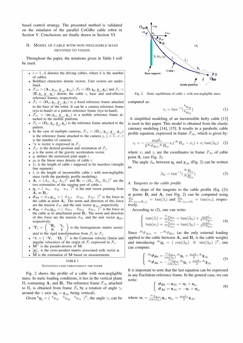
IV. VISION-BASED CONTROLA. Control

Visual servoing is based on the so-called interaction matrixLs which relates the instantaneous relative Cartesian motionτ between the mobile platform and the scene to the timederivative of the vector s of the visual primitives used forregulation [17] (s = Lsτ ). According to the nature of thevisual primitives, there exist many visual servoing techniquesranging from position-based visual servoing [18], [19] toimage-based visual servoing [4], [20], most of them beingbased on point features. One can also find other visualprimitives such as lines [21] or image moments [22].

As the instantaneous inverse kinematic model (10) de-pends on the platform pose, we choose position-based vi-sual servoing in the 3D pose form [18], [19], [23]: s =( st sw )T .

Consider Fm and Fm∗ the current and the desired mobileframe locations, respectively. st = mtm∗ is the translationerror between Fm and Fm∗ and sw = uθ, where u is theaxis and θ is the angle of the rotation matrix mRm∗ .

The interaction matrix associated to the pose can bewritten as [23], [24]:

Ls =

(−I3 [mtm∗ ]×03 −Lw

)(35)

where• Lw = I3 − θ

2 [u]× +(

1− sinc(θ)

sinc2( θ2 )

)[u]2×

• sinc(θ) = sin(θ)θ and mτm = mτm/m∗ = mτm/f

Control law mDm+

-

s

l.

Multiple-camera

Tension sensor

uAi

s *

Fig. 3. Visual servoing of a cable-driven parallel robot

To regulate the error between the current primitive vector sand the desired one s∗ = 0, one can consider the exponentialdecay s = −λs. The vision-based control (Fig. 3) can thenbe expressed as:

mτm = −λLs

+s (36)

With fτe = Dtmτm and using (36), (10) becomes:

q = mDmmτm = −λmDmLs

+s (37)

where Dt =(

fRmfRm[m

−−→Em]×

03fRm

)and mDm = 1

rcDaDt.

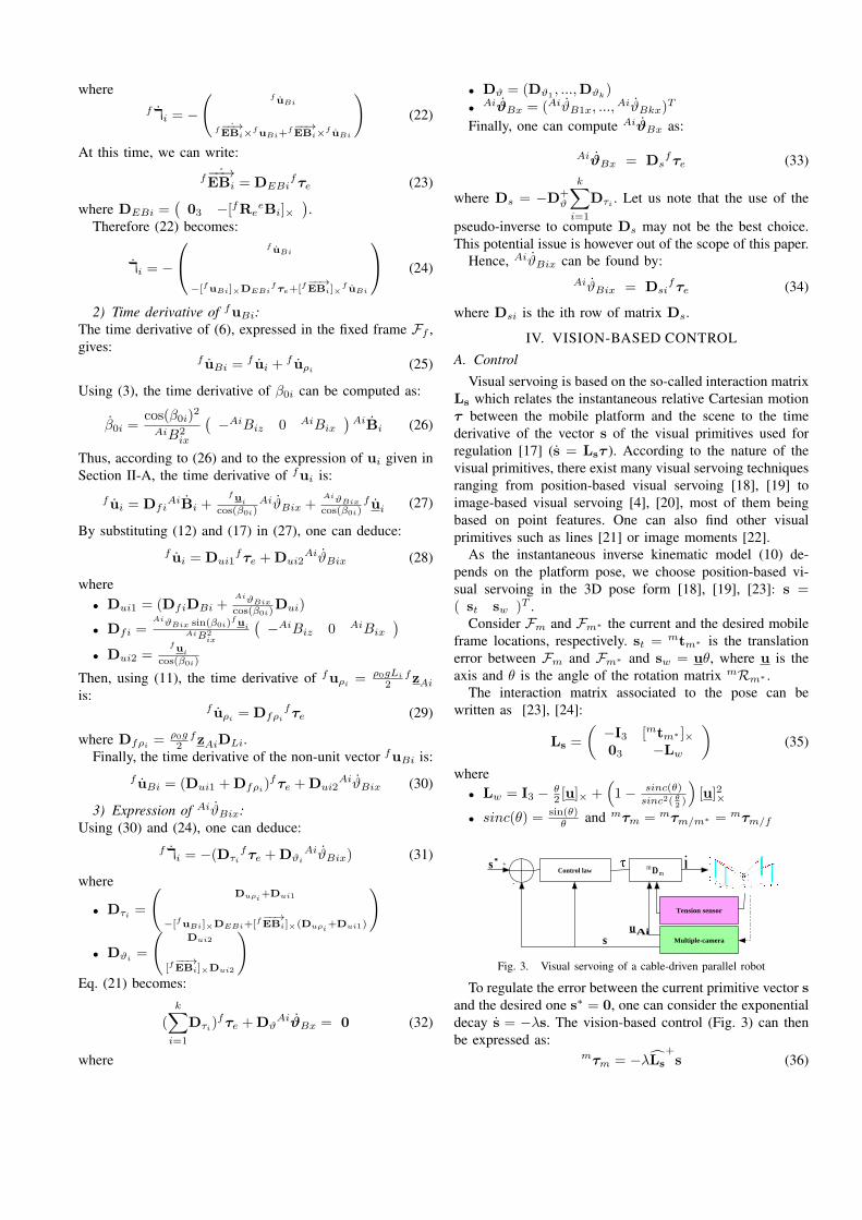
B. Examples of measured variables and parameters to iden-tify

Note that the instantaneous inverse kinematic model (10)depends on fTm, the rigid transformation between themobile and the fixed frame which defines the pose of theplatform. It depends also on the tangents fuAi to the cablesat their drawing points, which we plan to measure by vision,and on some constant (calibration) parameters (bAi, eBi, thetransformations mTe and fTb). Let us also note that onlyinformation from the vision sensor are used to define theinteraction matrix given in (35), using mTm∗ = mTf

fTm∗ .We plan to use 12 cameras. 4 cameras are used to

measure the pattern position (one at the top of each post).Additionally, 4 stereo pairs should allow us to measure thetangent direction at the cable drawing points. This particularsetup is not the only possible one but has been selectedbased on practical constraints. All kinematic parameters areexpressed in a reference frame Ff = Fcj attached to thebase frame.

Pattern

End Effector

Base

e Tp

ciTp

ciTb

Referencecamera:Cj

ciuAi

Fig. 4. A simulated CoGiRo robot

In the instantaneous inverse kinematic model (10), weneed to define the rotation AiRb which depends on the angleγi as shown in (1). This angle can also be computed usingγi = tan−1(

buAiybuAix

), where buAi = bRffuAi. We need also

the angle β0i defined in (3). This angle can be computedusing the following expressions of the attachment point Bi:

AiBi = AiRb(bRf

fBi + btf ) + AitbfBi = fRm

mBi + ftm(38)

where fRm and ftm can be measured by vision and mBi

is a constant parameter.The instantaneous inverse kinematic model (10) depends

also on the length Li =‖ f−−−→AiBi ‖ of cable i supposed to

be massless (straight line) and on the component AiϑBix ofthe force applied to the cable at its attachment point Bi.

Using (6), the non-unit vector fuBi can be computed as:fuBi = fϑBi = −AiϑAifuAi + ρ0gLi

fzAi (39)

where fzAi = fRbbzAi and AiϑAi is given by a tension

sensor (possibly indirectly).Consequently, using AiϑBi = AiRb

bRffϑBi, one can

compute AiϑBix = AixTAiAiϑBi.

V. SIMULATION RESULTS

The vision-based control strategy introduced in the pre-vious section is validated by means of a CoGiRo cable-driven parallel robot simulation (Fig. 4). CoGiRo is a 6-DOFlarge-dimension parallel cable-driven robot. It has a movingplatform (end-effector) connected to a fixed base by 8 drivingcables of varying lengths li, i ∈ 1...8 (k = 8). Each cable(Fig. 4) is attached to the moving platform at point Bi andextends from the base at point Ai.

In the simulation, bE = (0, 0, 0)Tm and (θx, θy, θz)T =

(0, 0, 0)T defines the initial configuration of the CoGiRoplatform simulation. The desired one (Fig. 5) is bE∗ =(2, 1, 1)Tm and (θ∗x, θ

∗y, θ∗z)T = (0, 10, 20)T .

In a first simulation, we choose three geometric charac-teristic cases (dimensions: width x length x height) of theCoGiRo robot. Tab. II presents the angles dβi = βi − β0i(See Fig. 2 for the definition of these angles), in the desiredposition. dβi increases according to the dimensions of therobot which confirms that the cables can not be consideredas a straight lines segments, in the case of a large-dimensionparallel cable-driven robots.

Casei \dβi dβ1 dβ2 dβ3 dβ4 dβ5 dβ6 dβ7 dβ810.8x14x5.5m 0.7 0.6 1.8 1.0 0.4 1.2 1.0 1.5

16.2x22.2x8.3m 1.3 1.3 3.2 1.5 0.8 3.15 1.8 2.227x37.0x13.9m 2.5 2.5 5.3 2.6 1.6 6.2 3.3 3.475x98.0x38.9m 5.7 5.4 8.3 5.5 4.2 9.4 6.3 6.9

TABLE IIEVOLUTION OF dβi = βi − β0i (DEGREES).

Fig. 5. Desired (left) and initial (right) position of the CoGiRo robot.

In a second simulation, we choose the dimensionsof the real CoGiRo robot (10.8 x 14 x 5.5 m(width x length x height)). To show the robustness ofthe proposed vision-based control, we added noise to theestimation of the Cartesian pose fTm. We define at each timea sample random noise for translation with maximal valueof 5 cm. We also added noise to the rotation angles, withamplitude of 2. Assuming that the directions of the tangentsto the cable curves at their drawing points is essentially a unitvector, the added noise can be modeled by a rotation of theunit vector in each direction. Consequently, we define at eachtime a sample random rotation axis and a positive rotationangle with maximal amplitude of 0.2.

Fig. 6 shows a potentially good robustness. As expected,the Cartesian errors converge exponentially to final errorsdisplayed in Table III, with a perfect decoupling. The 3Dtrajectory of the mobile platform (Fig. 7) is linear in the fixedreference frame Ff = Fcj , which confirms the properties ofthe 3D pose visual servoing.

Table III presents mean values and standard deviationsof the final error vector norm. These accuracy results aredeemed satisfactory enough for such a large-dimension par-allel robot.

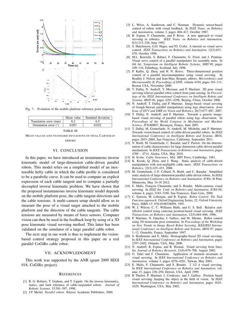
Fig. 6. Evolution of the Cartesian errors.

Fig. 7. Evolution of the mobile platform reference point trajectory.

Mean value Standard deviationTranslation error (mm) 8.2 6.5

Orientation error (°) 0.051 0.032

TABLE IIIMEAN VALUES AND STANDARD DEVIATIONS OF FINAL CARTESIAN

ERRORS

VI. CONCLUSION

In this paper, we have introduced an instantaneous inversekinematic model of large-dimension cable-driven parallelrobots. This model relies on a simplified model of an inex-tensible hefty cable in which the cable profile is consideredto be a parabolic curve. It can be used to compute an explicitexpression of each cable tangent and to compute a partiallydecoupled inverse kinematic problem. We have shown thatthe proposed instantaneous inverse kinematic model dependson the mobile platform pose, the cable tangent directions andthe cable tensions. A multi-camera setup should allow us tomeasure the pose of a visual target attached to the mobileplatform and the direction of the cable tangents. The cabletensions are measured by means of force sensors. Computervision can then be used in the feedback loop by using of a 3Dpose kinematic visual servoing method. This latter has beenvalidated on the simulator of a large parallel cable robot.

The next step in our work is thus to implement the vision-based control strategy proposed in this paper on a realparallel CoGiRo cable robot.

VII. ACKNOWLEDGMENT

This work was supported by the ANR (grant 2009 SEGI018, CoGiRo project).

REFERENCES

[1] R. G. Roberts, T. Graham, and T. Lippitt. On the inverse kinematics,statics, and fault tolerance of cable-suspended robots. Journal ofRobotic Systems, 15:581–597, 1998.

[2] J.P. Merlet. Parallel robots. Kluwer Academic Publishers, 2000.

[3] L. Weiss, A. Sanderson, and C. Neuman. Dynamic sensor-basedcontrol of robots with visual feedback. In IEEE Trans. on Roboticsand Automation, volume 3, pages 404–417, October 1987.

[4] B. Espiau, F. Chaumette, and P. Rives. A new approach to visualservoing in robotics. IEEE Trans. on Robotics and Automation,8(3):313–326, June 1992.

[5] S. Hutchinson, G.D. Hager, and P.I. Corke. A tutorial on visual servocontrol. IEEE Transactions on Robotics and Automation, 12(5):651–670, October 1996.

[6] M.L. Koreichi, S. Babaci, F. Chaumette, G. Fried, and J. Pontnau.Visual servo control of a parallel manipulator for assembly tasks. In6th Int. Symposium on Intelligent Robotic Systems, SIRS’98, pages109–116, Edimburg, Scotland, July 1998.

[7] P. Kallio, Q. Zhou, and H. N. Koivo. Three-dimensional positioncontrol of a parallel micromanipulator using visual servoing. InBradley J. Nelson and Jean-Marc Breguet, editors, Microrobotics andMicroassembly II, Proceedings of SPIE, volume 4194, pages 103–111,Boston USA, November 2000.

[8] T. Dallej, N. Andreff, Y. Mezouar, and P. Martinet. 3D pose visualservoing relieves parallel robot control from joint sensing. In Proceed-ings of the IEEE International Conference on Intelligent Robots andSystems, IROS’06, pages 4291–4296, Beijing, China, October 2006.

[9] N. Andreff, T. Dallej, and P. Martinet. Image-based visual servoingof Gough-Stewart parallel manipulators using legs observation. JointIssue of IJCV and IJRR on Vision and Robotics, 26(7):677–687, 2007.

[10] T. Dallej, N. Andreff, and P. Martinet. Towards a generic image-based visual servoing of parallel robots using legs observation. InProceedings of the World Congress in Mechanism and MachineScience, IFToMM07, Besancon, France, June 2007.

[11] T. Dallej, M. Gouttefarde, N. Andreff, M. Michelin, and P. Martinet.Towards vision-based control of cable-driven parallel robots. In IEEEInternational Conference on Intelligent Robots and Systems, IROS,pages 2855–2860, San Francisco, California, September 2011.

[12] N. Riehl, M. Gouttefarde, C. Baradat, and F. Pierrot. On the determi-nation of cable characteristics for large dimension cable-driven parallelmechanisms. In IEEE Transactions on Robotics and Automation, pages4709 – 4714, Alaska, USA, May 2010.

[13] H. Irvine. Cable Structures. MA: MIT Press, Cambridge, 1981.[14] K. Kozak, Q. Zhou, and J. Wang. Static analysis of cable-driven

manipulators with non-negligible cable mass. IEEE Transactions onRobotics, 22(3):425–433, 2006.

[15] M. Gouttefarde, J.-F. Collard, N. Riehl, and C. Baradat. Simplifiedstatic analysis of large-dimension parallel cable-driven robots. In IEEEInternational Conference on Robotics and Automation, ICRA, St Paul,Minnesota, May 14-18 2012.

[16] E. Malis, Francois Chaumette, and S. Boudet. Multi-cameras visualservoing. In IEEE Int. Conf. on Robotics and Automation, ICRA’00,volume 4, pages 3183–3188, San Francisco, Etats-Unis, 2000.

[17] C. Samson, M. Leborgne, and B. Espiau. Robot Control: The TaskFunction approach. Oxford Engineering Series, 22, Oxford UniversityPress, ISBN-13: 978-0198538059, 1991.

[18] W. J. Wilson, C. C. Williams Hulls, and G. S. Bell. Relative end-effector control using cartesian position-based visual servoing. IEEETransactions on Robotics and Automation, 12(5):684–696, 1996.

[19] P. Martinet, N. Daucher, J. Gallice, and M. Dhome. Robot controlusing 3D monocular pose estimation. In Proceedings of the Workshopon New Trends in Image Based Robot Servoing, IEEE/RSJ Interna-tional Conference on Intelligent Robots and Systems, IROS’97, pages1–12, Grenoble, France, September 1997.

[20] S. Benhimane and E. Malis. Homography-based 2D visual servoing.In IEEE International Conference on Robotics and Automation, pages2397–2402, Orlando, USA, May 2006.

[21] N. Andreff, B. Espiau, and R. Horaud. Visual servoing from lines.Int. Journal of Robotics Research, 21(8):679–700, August 2002.

[22] O. Tahri and F. Chaumette. Application of moment invariants tovisual servoing. In IEEE International Conference on Robotics andAutomation, volume 3, pages 4276–4281, Taiwan, May 2003.

[23] E. Malis, F. Chaumette, and S. Boudet. 2 1/2 d visual servoing.In IEEE International Conference on Robotics and Automation, vol-ume 15, pages 238–250, Detroit, USA, April 1999.

[24] B Thuilot, P. Martinet, L Cordesses, and J. Gallice. Position basedvisual servoing: keeping the object in the field of vision. In IEEEInternational Conference on Robotics and Automation, pages 1624–1629, Washington, USA, May 2002.