Vision-based estimation and robot control
129
HAL Id: tel-00411412 https://tel.archives-ouvertes.fr/tel-00411412 Submitted on 27 Aug 2009 HAL is a multi-disciplinary open access archive for the deposit and dissemination of sci- entific research documents, whether they are pub- lished or not. The documents may come from teaching and research institutions in France or abroad, or from public or private research centers. L’archive ouverte pluridisciplinaire HAL, est destinée au dépôt et à la diffusion de documents scientifiques de niveau recherche, publiés ou non, émanant des établissements d’enseignement et de recherche français ou étrangers, des laboratoires publics ou privés. Vision-based estimation and robot control Ezio Malis To cite this version: Ezio Malis. Vision-based estimation and robot control. Automatic. Université Nice Sophia Antipolis, 2008. tel-00411412
Transcript of Vision-based estimation and robot control

HAL Id: tel-00411412https://tel.archives-ouvertes.fr/tel-00411412
Submitted on 27 Aug 2009
HAL is a multi-disciplinary open accessarchive for the deposit and dissemination of sci-entific research documents, whether they are pub-lished or not. The documents may come fromteaching and research institutions in France orabroad, or from public or private research centers.
L’archive ouverte pluridisciplinaire HAL, estdestinée au dépôt et à la diffusion de documentsscientifiques de niveau recherche, publiés ou non,émanant des établissements d’enseignement et derecherche français ou étrangers, des laboratoirespublics ou privés.
Vision-based estimation and robot controlEzio Malis
To cite this version:Ezio Malis. Vision-based estimation and robot control. Automatic. Université Nice Sophia Antipolis,2008. �tel-00411412�

HABILITATION A DIRIGER DES RECHERCHES
Presentee a
l’Universite de Nice-Sophia Antipolis
par
Ezio Malis
sur le theme :
Methodologies d’estimation et de commande
a partir d’un systeme de vision
Vision-based estimation and robot control
Soutenue le 13 Mars 2008 devant le jury compose de :
P. Tarek Hamel President
P. Alessandro De Luca RapporteurD. Bernard Espiau RapporteurP. Gregory Hager Rapporteur
D. Francois Chaumette ExaminateurP. Philippe Martinet ExaminateurD. Patrick Rives Examinateur


Table des matieres
Introduction 1
1 Modeling and problems statement 31.1 Rigid bodies and robot models . . . . . . . . . . . . . . . . . . . . . . . . 4
1.1.1 Rigid body kinematics . . . . . . . . . . . . . . . . . . . . . . . . 41.1.1.1 Representing pose and structure of a rigid body . . . . . 41.1.1.2 Velocity of a rigid body . . . . . . . . . . . . . . . . . . 5
1.1.2 Robot models . . . . . . . . . . . . . . . . . . . . . . . . . . . . . 61.1.2.1 Holonomic robots . . . . . . . . . . . . . . . . . . . . . . 61.1.2.2 Non-holonomic robots . . . . . . . . . . . . . . . . . . . 7
1.2 Image models . . . . . . . . . . . . . . . . . . . . . . . . . . . . . . . . . 71.2.1 Photometric models . . . . . . . . . . . . . . . . . . . . . . . . . 8
1.2.1.1 Non Lambertian surfaces . . . . . . . . . . . . . . . . . . 81.2.1.2 Lambertian surfaces . . . . . . . . . . . . . . . . . . . . 8
1.2.2 Projection models . . . . . . . . . . . . . . . . . . . . . . . . . . . 81.2.2.1 Central catadioptric cameras . . . . . . . . . . . . . . . 91.2.2.2 Pinhole cameras . . . . . . . . . . . . . . . . . . . . . . 9
1.3 Problems statement . . . . . . . . . . . . . . . . . . . . . . . . . . . . . . 101.3.1 Estimation from visual data . . . . . . . . . . . . . . . . . . . . . 10
1.3.1.1 Calibration of the vision system . . . . . . . . . . . . . . 121.3.1.2 Localization and/or mapping . . . . . . . . . . . . . . . 121.3.1.3 Self-calibration of the vision system . . . . . . . . . . . . 13
1.3.2 Control from visual data . . . . . . . . . . . . . . . . . . . . . . . 131.3.2.1 Design of vision-based control schemes . . . . . . . . . . 141.3.2.2 Design of vision-based control laws . . . . . . . . . . . . 15
2 Numerical analysis 172.1 Iterative solution of non-linear equations . . . . . . . . . . . . . . . . . . 18
2.1.1 Functional iteration methods for root finding . . . . . . . . . . . . 192.1.1.1 Definition of the convergence domain . . . . . . . . . . . 192.1.1.2 Definition of the order of convergence . . . . . . . . . . . 21
2.1.2 Standard iterative methods . . . . . . . . . . . . . . . . . . . . . 222.1.2.1 The Newton-Raphson method . . . . . . . . . . . . . . . 222.1.2.2 The Halley method . . . . . . . . . . . . . . . . . . . . . 23
2.1.3 Iterative methods with known gradient at the solution . . . . . . 25

Ezio Malis ii
2.1.3.1 The efficient Newton method . . . . . . . . . . . . . . . 252.1.3.2 The Efficient Second-order approximation Method . . . 27
2.2 Iterative solution of nonlinear systems . . . . . . . . . . . . . . . . . . . 292.2.1 Extension to systems of nonlinear equations . . . . . . . . . . . . 29
2.2.1.1 The multidimensional Newton method . . . . . . . . . . 302.2.1.2 The multidimensional Halley method . . . . . . . . . . . 312.2.1.3 The multidimensional Efficient Newton Method . . . . . 312.2.1.4 The multidimensional ESM . . . . . . . . . . . . . . . . 32
2.2.2 Generalization to nonlinear systems on Lie groups . . . . . . . . . 322.2.2.1 Functional iteration on Lie groups . . . . . . . . . . . . 322.2.2.2 Newton methods for nonlinear systems on Lie groups . . 332.2.2.3 The ESM for nonlinear systems on Lie groups . . . . . . 33
2.3 Optimization of nonlinear least squares problems . . . . . . . . . . . . . 342.3.1 The Newton optimization and approximated methods . . . . . . . 34
2.3.1.1 The Gauss-Newton method . . . . . . . . . . . . . . . . 352.3.1.2 The Efficient Gauss-Newton method . . . . . . . . . . . 352.3.1.3 The Steepest Descent method . . . . . . . . . . . . . . . 362.3.1.4 The Levemberg-Marquardt method . . . . . . . . . . . . 36
2.3.2 The ESM for nonlinear least squares optimization . . . . . . . . . 362.3.2.1 Approximated ESM . . . . . . . . . . . . . . . . . . . . 362.3.2.2 Comparison with standard optimization methods . . . . 37
2.3.3 Robust optimization . . . . . . . . . . . . . . . . . . . . . . . . . 412.3.3.1 The M-estimators . . . . . . . . . . . . . . . . . . . . . . 412.3.3.2 The iteratively re-weighted least squares . . . . . . . . . 42
3 Vision-based parametric estimation 433.1 Feature-based methods . . . . . . . . . . . . . . . . . . . . . . . . . . . . 44
3.1.1 Features extraction . . . . . . . . . . . . . . . . . . . . . . . . . . 443.1.1.1 Accuracy . . . . . . . . . . . . . . . . . . . . . . . . . . 443.1.1.2 Repeatability . . . . . . . . . . . . . . . . . . . . . . . . 44
3.1.2 Features matching . . . . . . . . . . . . . . . . . . . . . . . . . . 453.1.2.1 Descriptors . . . . . . . . . . . . . . . . . . . . . . . . . 453.1.2.2 Similarity measures . . . . . . . . . . . . . . . . . . . . . 45
3.1.3 Parametric estimation . . . . . . . . . . . . . . . . . . . . . . . . 453.1.3.1 Calibration of the vision system . . . . . . . . . . . . . . 463.1.3.2 Localization and/or mapping . . . . . . . . . . . . . . . 473.1.3.3 Self-calibration of the vision system . . . . . . . . . . . . 50
3.2 Direct methods . . . . . . . . . . . . . . . . . . . . . . . . . . . . . . . . 523.2.1 Incremental image registration . . . . . . . . . . . . . . . . . . . . 53
3.2.1.1 Generic warping model . . . . . . . . . . . . . . . . . . . 543.2.1.2 Generic photometric model . . . . . . . . . . . . . . . . 593.2.1.3 Experimental results . . . . . . . . . . . . . . . . . . . . 60
3.2.2 Localization and/or Mapping . . . . . . . . . . . . . . . . . . . . 643.2.2.1 Monocular vision . . . . . . . . . . . . . . . . . . . . . . 65

iii Contents
3.2.2.2 Stereo vision . . . . . . . . . . . . . . . . . . . . . . . . 653.2.2.3 Experimental results . . . . . . . . . . . . . . . . . . . . 66
4 Vision-based robot control 714.1 Design of image-based control laws . . . . . . . . . . . . . . . . . . . . . 72
4.1.1 Analogies between numerical optimization and control . . . . . . 724.1.1.1 Standard control laws . . . . . . . . . . . . . . . . . . . 734.1.1.2 Standard optimization methods . . . . . . . . . . . . . . 73
4.1.2 The ESM for vision-based control . . . . . . . . . . . . . . . . . . 744.1.2.1 Improving image-based visual servoing schemes . . . . . 744.1.2.2 Stability and robustness analysis . . . . . . . . . . . . . 75
4.2 Design of robust visual servoing schemes . . . . . . . . . . . . . . . . . . 764.2.1 Increasing the robustness of image-based approaches . . . . . . . 76
4.2.1.1 A new class of visual servoing schemes . . . . . . . . . . 764.2.1.2 Direct visual servoing . . . . . . . . . . . . . . . . . . . 80
4.2.2 Beyond standard vision-based control approaches . . . . . . . . . 864.2.2.1 Visual servoing invariant to camera intrinsic parameters 864.2.2.2 Controlled visual simultaneous localization and mapping 89
Conclusion and future research 91
Appendix : Resume en francais 95Introduction . . . . . . . . . . . . . . . . . . . . . . . . . . . . . . . . . . . . . 95Activites de recherche . . . . . . . . . . . . . . . . . . . . . . . . . . . . . . . 96Conclusion . . . . . . . . . . . . . . . . . . . . . . . . . . . . . . . . . . . . . . 105
Bibliography 109

Ezio Malis iv
Introduction
The conception of full autonomous robotic systems is an enduring ambition for hu-mankind. Nowadays theoretical and technological advances have allowed engineers toconceive complex systems that can replace humans in many tedious or dangerous ap-plications. However, in order to considerably enlarge the flexibility and the domain ofapplications of such autonomous systems we still need to face several scientific problemsat the crossroad of many domains like for example artificial intelligence, signal processingand non-linear systems control.
Amidst these challenges, the perception of the environment and the interaction ofrobotic systems with the environment are fundamental problems in the design of suchautonomous systems. Indeed, the performance of an autonomous robot not only dependson the accuracy, duration and reliability of its perception but also on the ability to use theperceived information in automatic control loops to interact safely with the environmentdespite unavoidable modeling and measurement errors. Thus, automatic environment sen-sing and modeling, and robust sensor-based robot control are central scientific issues inrobotics.
Several exteroceptive sensors are commonly used in robotics : contact sensors (e.g.force sensors, tactile sensors), GPS, sonars, laser telemeters, vision sensors, and even ol-factory sensors. However, artificial vision is of particular importance and interest, mainlydue to its versatility and extended range of applicability. It can be used both for the per-ception and modeling of the robot’s environment and for the control of the robot itself. Inthis context, the spectrum of research is vast and I will focus on vision-based estimationand control problems. Vision-based estimation refers to the methods and techniques de-dicated to the extraction of the information that can be useful not only for the modelingof the environment but also for robot control. In the case of robotic applications, majorchallenges are to increase the efficiency, the accuracy and the robustness of the estimationfrom visual data. Vision-based control refers to the methods and techniques dedicatedto the use of visual information in automatic control loops. The challenges are to choosethe appropriate visual information and to design stable control laws that are robust tomodeling and measurement errors.
The objective of this document is to review, analyze and discuss my research workon these topics during the last ten years : two years as a Research Associate at the

Ezio Malis 2
University of Cambridge (United Kingdom) and eight years as a Research Scientist atINRIA Sophia-Antipolis (France). In order to acknowledge the contributions from all thecolleagues and students that have collaborated with me, I have tried as far as possible tocite all our common publications. The document is divided into four chapters :
– Chapter 1 : Modeling and Statement of Research Problems.
This introductory chapter is dedicated to presenting, as generally as possible, thevision-based estimation and control problems that have been considered by compu-ter vision and robotic researchers. I will start with general models that can be usedto classify and discuss the possible problems in parametric estimation and robotcontrol. However, in order to establish the basis for the more specific problems thatI will address in the rest of the document, I also briefly describe the specific modelsand assumptions that are commonly considered in the literature.
– Chapter 2 : Numerical Analysis.
This chapter considers numerical analysis methods that can be applied both tovisual parametric estimation and vision-based control. Our research work has focu-sed on methods which suppose that the parametric functions are differentiable. Themain contribution has been to propose a new numerical method called the EfficientSecond-order approximation Method (ESM). The main advantage of this methodis that, when applicable, it has a faster convergence rate and larger convergencedomain than standard numerical methods. Thus, it can be used to improve theparametric estimation and control from visual data.
– Chapter 3 : Vision-based parametric estimation.
This chapter details the vision-based parametric estimation problems that I haveaddressed. Our research work has focused on monocular and stereo vision systemscomposed by central cameras. The main contribution has been to propose efficientmethods to solve the image registration problem (visual tracking) and the pro-blems of localization and/or mapping. These methods have been designed to meetthe requirements of efficiency, accuracy and robustness needed in real-time roboticapplications.
– Chapter 4 : Vision-based robot control.
This chapter details the vision-based robot control problems that I have addres-sed. Our research work has focused on vision-based control of robots that can beconsidered as ideal Cartesian motion devices (such as for example omnidirectionalmobile robots or robot manipulators). The main contribution has been the designof robust vision-based control schemes that do not need an exact measure of theintrinsic parameters of the vision system and that do not need any “a priori” know-ledge of the structure of the observed scene. A particular emphasis has been placedon the theoretical analysis of the robustness of the control laws with respect toerrors on the uncertain parameters.

Chapitre 1
Modeling and problems statement
The research work presented in this document is related to both computer visionand automatic control. Indeed, my main objective has been to design robust methodsto control a robot evolving autonomously in natural environments using real-time visionsystems. In order to control the robot, we must not only be able to find its location withrespect to the environment but we may also need to recover a representation of the envi-ronment itself. In this context, another objective of my research work has been devotedto real-time parametric estimation from visual data. The aim of this chapter is to givea general statement of the vision-based estimation and control problems that have beenconsidered by computer vision and robotic researchers. A more detailed description ofour contributions will be presented in Chapter 2, Chapter 3 and Chapter 4.
For both parametric estimation and control objectives, it is extremely important tohave simple and accurate models of the robot, the environment and of the vision system.Although the ideal objective would be to control any complex system in any unknownenvironment with any vision system, such a general solution is out of reach. Thus, onlylimited models are currently used. The objective of this chapter is not only to introducethese models but also to understand what their limits are in terms of describing the reality.
The present chapter is organized as follows. First of all, I briefly introduce the modelsthat are considered in this document : the representation of the pose and of the structureof rigid objects, their kinematics, as well as some robot models. Then, I will describe ageneral model based on an ideal plenoptic function that is able to describe any possiblevision system. This function can be used to classify research work on parametric estima-tion from visual data and to analyze the related problems. Then, I will give a generaloverview of the research problems on vision-based robot control that I have considered.

Ezio Malis 4
1.1 Rigid bodies and robot models
1.1.1 Rigid body kinematics
Consider a rigid body in the Cartesian space (see Figure 1.1). A point P of therigid body can be represented with its Cartesian coordinates mr = (Xr, Yr, Zr) ∈ R
3
with respect to an inertial reference frame Fr equipped with a right-handed Cartesiancoordinate system (in such a coordinate system, a rotation from the ~x-axis to the ~y-axis(about the ~z-axis) is positive) which is attached to a point O. Let Fc be a current frameattached to a point C and freely moving with respect to the inertial frame Fr.
t = ~OC
P
R
n
O
C
~OP
~CP
Fig. 1.1 – Configuration of a rigid body.
1.1.1.1 Representing pose and structure of a rigid body
The current pose of the rigid body (position and orientation) with respect to themoving frame can be described by a (4×4) homogeneous transformation matrix rTc
containing the coordinates of the current frame Fc in the basis of the fixed frame Fr.The matrix rTc ∈ SE(3) (see for example [Warner 71, Varadarajan 74, Hall 03]) can bewritten as :
rTc =
[rRc
rtc
0 1
](1.1)
where rtc = ( ~OC)r ∈ R3 is the translation vector and rRc ∈ SO(3) is the rotation matrix
of frame Fc with respect to frame Fr. The matrix rTc tells us where the current frame Fc
is with respect to the reference frame Fr. Let mc = (Xc, Yc, Zc) ∈ R3 be the coordinates of
the same point P expressed in frame Fc. Using the homogeneous coordinates mr = (mr, 1)and mc = (mc, 1), the coordinates of the point P in the current frame Fc can be obtainedfrom the coordinates in the reference frame Fr :
mc = cTr mr (1.2)

5 Modeling and problems statement Chapter 1
where cTr = rTc−1. The change of coordinates in equation (1.2) can also be written for
non-homogeneous coordinates as follows :
mc = τ (cTr,mr) = cRr mr + ctr (1.3)
The three points O, C and P are coplanar. Thus we can obtain from equation (1.3) :
m⊤
r [rtc]×rRc mc = m⊤
r [rEc]× mc = 0 (1.4)
where the (3 × 3) matrix rEc = [rtc]×rRc is called the essential matrix.
When the point P belongs to a planar surface (see Figure 1.1) its coordinates satisfythe following equation :
n⊤
r mr = 1 (1.5)
where nr is a vector normal to the plane such that ‖nr‖ = 1/dr (dr being the distancebetween the plane and the point O). Thus, the point mr and mc are related by thefollowing equation :
mc = cHr mr (1.6)
where the (3×3) matrix cHr is called the homography matrix. This matrix can be writtenas follows :
cHr = cRr + ctr nr (1.7)
Note that if det(H) = 0 the plane passes through the origin of the current frame.
1.1.1.2 Velocity of a rigid body
Consider a (4×4) matrix Ac ∈ se(3) (see [Warner 71, Varadarajan 74, Hall 03]) Thismatrix contains the instantaneous rotation and translation velocity vectors ωc and νc
expressed in the current frame (i.e. the velocity of the frame Fc expressed in the currentframe itself) :
Ac =
[[ωc]× νc
0 0
](1.8)
The derivative of rTc can be written as :
rTc =
[rRc
rtc
0 0
]= rTcAc (1.9)
One may want to express the velocity of the current frame not in the coordinate system ofthe current frame itself but in the coordinate system of the reference frame. Let Ar ∈ se(3)be the velocity of the current frame expressed in the coordinates of the reference frame :
Ar =
[[ωr]× νr
0 0
](1.10)
The derivative of rTc can be written as :
rTc = ArrTc (1.11)

Ezio Malis 6
From equations (1.9) and (1.11) we can compute Ar as a function of Ac :
Ar = rTc AccTr (1.12)
Then, one can easily compute this very well known change of frame for the velocity :[νr
ωr
]=
[rRc [rtc]×
rRc
0 rRc
] [νc
ωc
](1.13)
The velocity of a point in the current frame can easily be calculated by deriving equa-tion (1.3) and using equation (1.9) :
mc = −νc + [mc]× ωc (1.14)
1.1.2 Robot models
In this document, I will consider robots for which the kinematic model can be writtenas follows :
x =m∑
i=1
uibi(x) (1.15)
where x ∈ Rn is a vector which contains local coordinates of the configurations space, ui
are the control inputs and bi(x) are the corresponding vector fields. I will now give twoexamples of models for holonomic and non-holonomic robots.
1.1.2.1 Holonomic robots
Holonomic robots (like manipulator or omnidirectional mobile robots) can be viewedas ideal Cartesian motion devices. Let me set in this case x = (t, r) ∈ R
6, where t ∈ R3
is the translation vector and r ∈ R3 is a local representation of the rotation. Thus, the
vector x is a local parametrization of SE(3)). Let me use the angle-axis representationr = θu due to its links with Lie algebra (see [Warner 71], [Varadarajan 74], [Hall 03]).The matrix rTc can be written as a function of x as follows :
rTc = T(x) =
[exp([r]
×) t
0 1
](1.16)
The derivative of the matrix rTc can be written :
rTc = rTc Ac (1.17)
and thus Ac = T(x)−1T(x) (see equation 1.8). Let me set v = (νc,ωc) ∈ R6. Rearranging
equation (1.17), we can write :x = B(x)v (1.18)
where B(x) is a (6 × 6) matrix. We can identify this equation with equation (1.15) bysetting m = n = 6, ui = vi and bi(x) being the i-th column of the matrix B(x). I willsuppose that a low level controller exists such that the control input of the robot is theCartesian velocity v.

7 Modeling and problems statement Chapter 1
1.1.2.2 Non-holonomic robots
Non-holonomic robots have kinematic constraints on the velocity in the configurationspace. This means that m < n in equation (1.15). For example, if we consider a unicycleevolving on a planar surface we can set m = 2 and suppose that the vector x ∈ R
3 is a localrepresentation of SE(2). Non-holonomic robots are generally critical non-linear systems.Some tasks that can easily be accomplished by holonomic robots become very complex forthese systems. For example, positioning a non-holonomic robot can be extremely difficulteven if the robot is controllable [Morin 04].
1.2 Image models
The formation of an image depends on the geometry of the scene and its photometricproperties, on the distribution of the illumination sources and their photometric proper-ties as well as on the intrinsic characteristics of the image sensor and its position andorientation with respect to the scene.
An image sensor is a device that captures light and converts it to an electric signal.Let me suppose that the device is composed of a rectangular grid of photo-detectorsthat may also be able to measure light wavelength (i.e. colors). Thus, an image can beconsidered as a (su × sv × sc) tensor where sv is the number of pixel rows, su is thenumber of pixel columns and sc is the number of color channels. A common assumptionis to suppose that the discrete signal measured by the image sensor has been sampled froma smooth continuous-time signal. Let pc = (u, v) be the (2×1) vector in R
2 containingthe coordinates of a point in the sensor grid. Each point pc corresponds to an entry ofthe tensor :
I(φ,pc) (1.19)
where φ is a vector containing some photometric parameters (see Section 1.2.1 for details).We suppose that the light measured at point pc comes from a visible 3D point of thescene mc. Thus, we suppose that a smooth projection function π exists such that :
pc = π(κ,mc) (1.20)
where κ are some projection parameters that depend on the camera model (see Sec-tion 1.2.2). From equation (1.3) we can write mc as a function of the coordinates mr ofthe same point in the inertial reference frame and of the matrix rTc which allows thecoordinate transformation from the current frame to the inertial reference frame. Plug-ging equations (1.20) and (1.3) into (1.19) and grouping all the coordinates mr of the 3Dpoints in a single vector γ = (m1,m2, . . . ,mp) we obtain the following function :
ψ(φ,κ,γ,T) = {I(φ,π(κ, τ (T,m1))), . . . ,I(φ,π(κ, τ (T,mp)))} (1.21)
This function can be interpreted as a generalization of the plenoptic function proposedby [Adelson 91]. The general plenoptic mapping in equation (1.21) is an ideal functionthat describes everything that is visible from any pose in space, for any camera, for anystructure and for any illumination (and at any time).

Ezio Malis 8
I will give now some examples of standard models that are generally used to describethe plenoptic function. These models will be considered in the rest of the document.
1.2.1 Photometric models
1.2.1.1 Non Lambertian surfaces
According to major illumination models, the luminance at a particular pixel p is dueto diffuse, specular and ambient reflections :
I(φ,pc) = Is(φs,pc) + Id(φd,pc) + Ia (1.22)
where φ = (φs,φd) and φs and φd are parameters that depend on the illumination model(e.g. [Blinn 77], or [Cook 82]). The ambient intensity Ia is constant. The parametersφs, defining the specular reflections, also depend on the position of the image sensorwith respect to the observed surface. The diffusion parameters φd depend amongst otherparameters (e.g. the albedo) on how the surface faces the light sources.
1.2.1.2 Lambertian surfaces
Lambertian surfaces or ”ideal diffuse surfaces” are surfaces for which the image in-tensity of a pixel depends only on how the surface faces the light sources (i.e. there areno specular reflexions). Equation (1.22) can be written
I(φ,pc) = Id(φd,pc) + Ia, (1.23)
where φ = φd contains the diffusion parameters only. Thus, if we observe a static envi-ronment and the light sources are fixed, then two corresponding pixels in two differentimages will have the same intensity. This particular case corresponds to the well known“Brightness Constancy Assumption”.
1.2.2 Projection models
As already mentioned we suppose that a parametric smooth function π exists suchthat :
pc = π(κ,mc) = π(κ, τ (cTr,mr))
The parameters contained in the vector κ are called the camera intrinsic parameters anddepend on the considered projection model. There are two main groups of cameras :
– Central cameras : for a central camera all the light rays forming the image meet atthe same point called the center of projection.
– Non-central cameras : for a non central camera the light rays forming the imagemeet in more that one center of projection. The set of centers of projection is calleda caustic and it determines the characteristics of the camera.
In this document, I will consider central cameras only. I will now describe the modelsthat are generally used for this type of camera.

9 Modeling and problems statement Chapter 1
1.2.2.1 Central catadioptric cameras
Using the unified model for central catadioptric cameras proposed by [Baker 99],[Geyer 00], and [Barreto 02], the image point pc is obtained by a projection of mc onto aunit sphere, followed by a map projection onto a virtual plane, followed by a coordinatedistortion and finally followed by an affine coordinate transformation. The point mc canbe projected on the unit sphere S in a 3D point having coordinates sc = (Xs, Ys, Zs) :
sc =mc
‖mc‖(1.24)
Then, the projection from a point sc to a 2D image point pc can be described by aprojective mapping c : S
2 7→ R2 :
pc = c(κ, sc)
where κ is a vector which contains the camera intrinsic parameters. I will suppose thatthe map c is invertible and sc = c−1(κ,pc). For example, the function c for a genericcamera can be written as follows. The map projection of the point sc on the sphere (froma projection point Cp) to a point qc = (x, y) on a virtual plane can be written :
qc = h(ξ, sc) =
(Xs
Zs − ξ,
Ys
Zs − ξ
)(1.25)
where ξ is a parameter which defines the characteristic of the camera : The point qc maybe distorted to the point qd = (xd, yd) :
qd = d(δ,qc)
where δ is a vector containing the parameter of the distortion model. Typical distortionmodels are given in [Weng 92]. Finally, the virtual point is projected on the image planeinto the point pc = (u, v) :
pc = k(ρ,qd) = (ρ1 xd + ρ2 yd + ρ3, ρ4 yd + ρ5) (1.26)
It has been shown by [Courbon 07] that this model can also approximate well severalprojection models for central dioptric cameras (fish-eye cameras).
1.2.2.2 Pinhole cameras
In the particular case when there is no mirror ξ = 0 and no image distortion δ = 0 thecamera is a pinhole. Using homogeneous coordinates, the equation (1.26) can be writtenas :
pc= Kq
c(1.27)
where K is a (3 × 3) triangular matrix containing the camera intrinsic parameters :
K =
f f s u0
0 f r v0
0 0 1
(1.28)

Ezio Malis 10
where (u0, v0) are the coordinates of the principal point (in pixels), f is the focal lengthmeasured in pixels, s is the skew and r is the aspect ratio. Note that equation 1.27 canalso be written :
p ∝[K 0
]m
This projection model has been widely used since it is a very good approximation ofmany commercial cameras with good quality lenses.
1.3 Problems statement
The principal objective of my research work has been to design robust methods forparametric visual estimation and for controlling a robot in large scale environments usinga vision system. The information acquired by the vision system can be described by anon-linear system of equations (see Section 1.1). The evolution of the state of the robotcan be described by a system of differential equations (see Section 1.2). Thus, in generalthe overall non-linear dynamic system can be represented by the following state spaceequations :
x(t) = g(x(t),u(t), t) (1.29)
y(t) = h(η(t),x(t)) (1.30)
where x is the state of the system, u is the control input, g is a smooth vector functiondescribing the evolution of the state of the system and y is the output vector representedby a smooth vector function h. The function h depends on the pose of the vision systemcontained in x but also on the camera intrinsic parameters and on the structure of theenvironment contained in the vector η. The problems related to the estimation of thisinformation from visual data are described in Section 1.3.1. Then, in Section 1.3.2 I willdiscuss the problems related to the stabilization of the non-linear dynamic system usingvisual information.
1.3.1 Estimation from visual data
The function h that describes the behavior of the output y of the vision system can berepresented using the general plenoptic function described in Section 1.2. Let me considerthe most general case where the vision system is composed of nc synchronized cameraswith varying intrinsic parameters (e.g. zooming cameras) that observe a non-rigid scene.In this case the output y(t) of the vision system contains a collection of images acquiredat the same time by all the cameras of the vision system. The output y(t) can be obtainedby rearranging all the nc plenoptic functions in a single vector :
y(t) = {ψ(φ1(t),κ1(t),γ(t),T2(t)), . . . ,ψ(φnc(t),κnc
(t),γ(t),Tnc(t))} (1.31)
Suppose we have a set of visual data y(ti) acquired at times ti, ∀i ∈ {1, 2, ni}, (i.e. acollection of images or a video sequence). Suppose also that we have a perfect modelof the plenoptic function (see Section 1.2). Thus, some parameters φk(ti), κk(ti), Tk(ti)

11 Modeling and problems statement Chapter 1
and mj(ti) exist such that I(φk(ti),π(κk(ti), τ (Tk(ti),mj(ti)))) = I ijk, ∀i, j, k. Thus,the problem of parameters estimation from the observed visual data is equivalent to thesolution of the following system of non-linear equations ∀i, j, k :
I(φk(ti),π(κk(ti), τ (Tk(ti),mj(ti)))) = I ijk (1.32)
An exhaustive description of all possible methods and algorithms that have been proposedto solve this non-linear problem is beyond the scope of this document. The reader mayrefer to numerous well-known textbooks like [Faugeras 93], [Hartley 00], [Faugeras 01][Ma 03]. Despite the impressive achievements of computer vision scientists, there stillexist three challenging sets of problems related to the solution of this non-linear systemof equations.
The first set of problems concerns the modeling of the plenoptic function. The parame-tric model of the plenoptic function is supposed to be perfect. Obviously, this assumptionis not true in general. Thus, the problem is how to find simple, accurate, and generalmodels of the plenoptic function. Simple means that only a few parameters are neededto represent the model. Accurate means that the model can fit the measures accurately.General means that the same model can be applied to most of the existing vision systems.
The second set of problems concerns data association. The photodetectors of theimaging device are supposed to instantaneously measure the light coming from an ideal3D point. These assumptions are not true in general since during the exposure timethe photodetectors integrate the light coming from a portion of a 3D surface. Whenthe shutter speed is not fast enough we can have blur on moving objects. Moreover, asthe pixel resolution of the imaging device is fixed, the intensity of the same portion ofa 3D surface will not always be measured by a single pixel. Even assuming that theshutter is almost instantaneous and the light is coming from an ideal 3D point, how dowe obtain a precise correspondence of the 3D coordinates mj(ti) and the pixel intensityI ijk ? Similarly, how we can obtain a precise correspondence of the intensity I ijk of oneimage point and the intensity of the corresponding points in the other images ? This lastproblem can be simplified assuming the visual data come from a video sequence acquiredwith a sufficiently fast frame rate. This allows us to suppose that two corresponding pixelsare adjacent in two consecutive images.
The third set of problems concerns the solution of the non-linear system. The plenopticfunction is supposed to be smooth and noiseless. This assumption is generally not truebut it allows us to use numerical methods that compute the derivatives of the function.Even supposing that the problem is well posed, how can we robustly and efficientlysolve the system of non-linear equations for real-time applications ? Robustness withrespect to aberrant measures (i.e. outliers) is necessary since it is impossible to obtaina perfect representation of the plenoptic function. Efficiency is extremely important forfast real-time application (like vision-based control) and it can be obtained in two ways.One possibility is to simplify the system of equations. For example we can eliminatesome of the unknowns to obtain a smaller nonlinear system (e.g. subspace methods ,invariance ...). The second possibility is to use efficient numerical methods for the solutionof the nonlinear system. Whatever the method used to solve the nonlinear system weneed to know if the problem is well posed. Computer vision and robotic scientists soon

Ezio Malis 12
realized that in this very general form the problem may not have a unique solution (notsurprisingly since inverse problems are generally not well posed). Typically, there aremore unknown parameters than equations. Thus, some additional constraints are addedto the original nonlinear system in order to obtain a well posed problem. The exhaustivedescription of all possible assumptions is out of the scope of this document. Howeversome of them are very common for many problems that are of interest for real-timeapplications. For example, a very usual assumption is to suppose that the camera observesa rigid Lambertian surface that is static with respect to the sources of illumination. Thisassumption allows us to considerably reduce the number of unknown parameters since wecan set φk(ti) = φ and mj(ti) = mj. Another technique to reduce the number of unknownparameters is regularization. For example, we can suppose that the observed scene ispiecewise planar or that it is composed of smooth surfaces. Temporal regularization isalso a common assumption (i.e. assuming that the parameters vary slowly in time orthat the collection of images comes from a video sequence). The estimation problem canalso become well posed if we assume that the true values of some parameters are alreadyknown “a priori”. Even if this may be a very strong assumption, this solution has beenwidely used. In the following sections I will detail three standard classes of problems thathave been considered by computer vision and robotic scientists.
1.3.1.1 Calibration of the vision system
One of the first problems addressed by robotic vision scientists has been the estimationof the intrinsic parameters of a vision system. The reason why these parameters deserveparticular attention is that in many applications they can be considered constant so thatthey can be estimated once and for all. Suppose that we observe several images of aknown rigid object (a calibration grid for example) and that the intrinsic parameters ofthe cameras are constant κk(ti) = κk (i.e. the cameras do not zoom). Since the objectis known the coordinates mj(ti) = mj of all the 3D points of the object are known in areference frame. Finally, suppose that we know that the intensity I ijk measured by eachimage sensor corresponds to the point mj. Thus, we can solve the following system ofnon linear equations :
I(φk(ti),π(κk, τ (Tk(ti),mj))) = I ijk (1.33)
This problem is called the “camera calibration problem” and several solutions have beenproposed in the literature. Even if only one image of a known grid can be sufficient tosolve the problem, several images are generally considered in order to obtain a preciseestimation of the parameters.
1.3.1.2 Localization and/or mapping
Suppose now that the camera intrinsic parameters have been recovered once and forall κk = κk and that we observed a rigid scene (i.e. mj(ti) = mj). Then one may beinterested to solve the simultaneous localization and mapping problem :
I(φk(ti),π(κk, τ (Tk(ti),mj))) = I ijk (1.34)

13 Modeling and problems statement Chapter 1
where the structure and the translations of the camera can be estimated only up to ascale factor if we do not have any additional constraint.
Another problem of interest in robotic vision is the reconstruction of the structurefrom known motion. Indeed, if a calibrated vision system is mounted on a well calibratedrobot we are able to measure the displacement Tk(ti) for each image. Thus the problembecomes :
I(φk(ti),π(κk, τ (Tk(ti),mj))) = I ijk (1.35)
Another problem of interest is the localization of the vision system when the model ofthe object is known. The localization can be obtained by solving the following system :
I(φk(ti),π(κk, τ (Tk(ti),mj))) = I ijk (1.36)
This problem is closely related to the camera calibration problem but here only thecamera displacement and the photometric parameters are unknown. The localization ofthe vision system can also be obtained if the structure mj is unknown but the visionsystem has multiple calibrated cameras (e.g. a calibrated stereo pair). In this case theposes of the cameras with respect to each other are known.
1.3.1.3 Self-calibration of the vision system
If we observe an unknown rigid object and the cameras’ intrinsic parameters are notconstant (e.g. if we consider zooming cameras) then the problem of estimating all possibleparameters is called the “camera self-calibration problem” :
I(φk(ti),π(κk(ti), τ (Tk(ti),mj))) = I ijk (1.37)
This problem is generally not well posed and it cannot always be solved. For example,consider the very simple case of a pinhole camera with constant camera parametersκk(ti) = κk observing a motionless Lambertian surface. The camera self-calibration pro-blem cannot be solved if the camera does not rotates. If all the camera intrinsic parametersvary with time then the problem cannot be solved even if the camera rotate. Note alsothat if we do not have any additional metric knowledge, the structure and the translationsof the cameras can be estimated only up to a scale factor
1.3.2 Control from visual data
The first step to controlling the robot using the visual information is to define the taskto be accomplished by the robot. There are several possible tasks that can be defined,for example to reach a reference position or a reference velocity. The definition of thetask also depends on the configuration of the vision system and on the type of robot.For example, the vision system can be mounted on the end-effector of the robot (thisconfiguration is called “eye-in-hand”) or not (this configuration is called eye-to-hand). Anexhaustive description of all possible tasks and configurations is beyond the scope of thisdocument. The reader may refer to numerous books, tutorials and surveys that have beenpublished on the subject, like [Hashimoto 93, Hutchinson 96, Malis 02b, Chaumette 06,

Ezio Malis 14
Chaumette 07]. Research in visual servoing initially focused on the problem of controllingthe pose of a camera, assuming that the camera can (locally) move freely in all directions.This is the case, for instance, when the camera is mounted on an omnidirectional mobilerobot, or on the end-effector of a classical manipulator endowed with (at least) 6 degreesof freedom. This is equivalent to viewing the robot as an ideal Cartesian motion device.The control part of the problem is then simplified since standard control techniques,like pure state feedback linearization, can be applied. The case of robotic vision-carrierssubjected to either nonholonomic constraints (like car-like vehicles) or underactuation(like most aerial vehicles) raises a new set of difficulties.
Consider now the case when the robot can be considered as an ideal Cartesian motiondevice. In order to simplify the discussion a specific task is considered here : positioninga holonomic robot with respect to a motionless object using the information acquired bya eye-in-hand vision system. Thus, the state of the system x is locally homeomorphic toSE(3) and the function g that describes the behavior of the state x can be modeled as inSection 1.1. The function h that describes the behavior of the output y can be modeledas in Section 1.2. Thus, the system of equations (1.29) can be rewritten as follows :
x(t) = B(x(t))v(t) (1.38)
y(t) = h(η(t),x(t)) (1.39)
where the velocity of the camera v(t) is the control input.
1.3.2.1 Design of vision-based control schemes
The design of a vision-based control scheme depends on how the task has been defined.For example, the positioning task can be defined directly in the Cartesian space as theregulation of the vector x(t). Without loss of generality, we can suppose that our objectiveis to regulate the vector x(t) to zero. In this case one must be able to estimate the currentcamera pose from image data. Using an approximation of the parameters η(t), one mustdesign a non-linear state observer ψ such that :
x(t) = ψ(η(t),h(η(t),x(t))) (1.40)
Obviously, in the absence of modeling errors we have η(t) = η(t) and thus the state can beperfectly estimated x (t) = ψ(η(t),h(η(t),x(t))) = x (t). The problem of reconstructingthe pose of the camera with respect to the object has been widely studied in the roboticvision community (see Chapter 3) and several solutions have been proposed. For example,if we have a calibrated monocular vision system we need an accurate model of the target.If we have a calibrated stereo system, the model of the target can be estimated on-lineby triangulation. The main limitation of this approach is that any modeling error mayproduce an error in the final pose.
In order to design vision-based control schemes that are more robust to modelingerrors, researchers have proposed using a “teaching-by-showing” approach where the re-ference pose is not given explicitly. Instead, a reference output y is acquired at the

15 Modeling and problems statement Chapter 1
reference pose (again we can suppose without loss of generality that the reference posecorresponds to x = 0) :
y = h(η, 0) (1.41)
where η contains the parameters at the time of the acquisition. Thus, we can build anerror function (not necessarily having the same size as the vector x) from image dataonly :
ǫ(t) = δ(h(η(t),x(t)),h(η, 0)) (1.42)
such that if (and only if) ǫ = 0 then x = 0. The design of such an error function is noteasy, especially if the parameters η(t) vary. Thus, a common assumption is to supposethat imaging conditions do not change η(t) = η. Even with such an assumption, thedesign of the error function is not easy and its choice may greatly influence the behaviorof the visual servoing. In particular, the influence of measurement noise can be verydifferent depending on the choice of the error function.
In the teaching-by-showing approach, the choice of the error function cannot be gene-rally decoupled from the design of the control law. Indeed, the same control law can havean unstable behavior with a given control error and a stable behavior with a differentcontrol error. Moreover, even if it is possible to compute the control error directly fromimage data, the design of a stable control law often needs an estimate of the parametersη.
1.3.2.2 Design of vision-based control laws
The design of control laws is a fairly standard problem in robotics when the poseof the camera can be estimated explicitly. However, it is worth noting that for criticalsystems the design of the control law is more difficult than for holonomic robots. Let meconsider here the design of control laws for the teaching-by-showing approach supposingthat imaging conditions do not change η(t) = η. After taking the time derivative of thecontrol error in equation (1.42) we obtain the following state equations :
ǫ(t) = L(η,x(t))v(t) (1.43)
y(t) = h(η,x(t))
where L is an interaction matrix that generally depends on the parameters η. The problemis to find an appropriate function k in order to ensure a stable control input :
v(t) = k(η,y(t),y) = k(η,h(η,x(t)),h(η, 0))
such that ǫ(t) → 0 when t → ∞ starting from an initial pose x0 = x(0). The challenge isto design stable control laws that depend as little as possible on the unknown parametersη. If an estimation η is needed, another challenge is to design stable control laws thatare robust to errors on the estimation of these parameters.
Ezio Malis 16
1.3.2.2.1 Stability and robustness
In ideal conditions (i.e. assuming no modeling and measurement errors) the control lawshould be at least locally stable. This is the minimal requirement in the design of vision-based control laws. However, it is also important to determine the “size” of the stabilitydomain. A very difficult problem is to design control laws with a large stability domain.The best would be to design globally stable control laws (i.e. the control error convergenceto zero whatever the starting position of the robot).
Another problem is the design of robust control laws. A control law can be called“robust” if it is able to perform the assigned stabilization task despite modeling andmeasurement errors. Determining the “size” of “admissible” errors is important in prac-tice. However, carrying out this type of analysis is usually technically quite difficult.Robustness is needed to ensure that the controlled system will behave as expected. It isan absolute requirement for most applications, not only to guarantee the correct execu-tion of the assigned tasks but also for safety reasons, especially when these tasks involvedirect interactions with humans (robotic aided surgery, automatic driving,...).
1.3.2.2.2 Visibility and Continuity
The aim of vision-based control techniques is to control a robot with the feedback comingfrom visual information. If the visual information gets out of the camera’s field of viewfeedback is no longer possible and the visual servoing must then be stopped. A very im-portant problem is to take into account this constraint in the design of the control law.This visibility problem is amplified when considering critical systems, like non-holonomicrobots, due to the restriction on the possible instantaneous motions of the robot.
Another problem related to the visibility appears when the target is partially occluded.In this case, if we suppose that sufficient information is still visible in order to achieve thetask, the problem is that the occlusion may perturb the computation of the control errorand/or the control law. Depending on how the control scheme has been defined somediscontinuities may appear. These discontinuities perturb and decrease the performancesof the control law.

Chapitre 2
Numerical analysis
Many parametric estimation problems can be solved by finding the solution of a systemof non-linear equations. When the system has more equations than unknowns it is usualto rewrite the problem as a nonlinear least squares optimization which is again solved byfinding the solution of another system of non-linear equations. In general, these nonlinearproblems do not have an analytical closed-form solution. Thus, an important researchsubject concerns the study of efficient iterative numerical methods. The objective of thischapter is to describe my contributions in this field.
Numerical methods have been widely studied in the literature. An exhaustive des-cription of them is beyond the scope of this document. In this chapter, the focus is onnumerical methods that make use of derivatives of the nonlinear functions involved in theproblems. Indeed, such methods have a strong link with automatic control methods. Thereader may refer to well-known textbooks like [Isaacson 66], [Dennis 83], [Quarteroni 00]which describe in detail most of the standard numerical methods. Besides the standardmethods, I will consider methods that use additional information on the derivatives atthe solution. In several robotic vision applications, such as for example parametric iden-tification or vision-based control, it is possible to measure or approximate this additionalknowledge. In this context, one important contribution has been to propose the EfficientSecond-order approximation Method (ESM) which has several advantages with respectto standard methods. The ESM has been successfully applied to vision-based estimation(see Chapter 3) and to vision-based robot control (see Chapter 4).
The chapter is organized as follows. First the problem of finding the solution of onenonlinear equation in one unknown is considered. The reason for studying the one-variableproblem separately is that it allows us to more easily understand the principles of thedifferent methods that have been proposed in the literature. For example, geometric inter-pretations of the methods can be plotted [Isaacson 66]. The extension to the multidimen-sional case (i.e. the solution of systems of nonlinear equations) is almost straightforward.Then, the generalization of the iterative methods to nonlinear systems defined on Liegroups is introduced. Finally, I will consider the optimization of a nonlinear least squaresproblem and its modification to increase robustness with respect to aberrant measure-ments.

Ezio Malis 18
2.1 Iterative solution of non-linear equations
In this section, I consider the problem of iteratively finding a root of the equation :
f(x) = 0 (2.1)
given the function f : D = (a, b) ⊆ R 7→ R and starting from an initial approximation x0
of a root x. The problem of how to find the initial approximation x0 is not easy to solvebut is very important since we will see that most of the iterative method will not work ifx0 is chosen too far from x. For simplicity, let me suppose that the function f(x) ∈ C∞
so that it can be expanded using a Taylor series about x :
f(x + x) = f(x) + g(x) x +1
2h(x) x2 +
1
6q(x∗) x3 (2.2)
where the last term is a third-order Lagrange remainder and x∗ ∈ (x, x) and the smoothfunctions g(x), h(x), and q(x) are defined as follows :
g(x) =df(x)
dx(2.3)
h(x) =d2f(x)
dx2(2.4)
q(x) =d3f(x)
dx3(2.5)
Suppose that x is a simple root of the equation (2.1), therefore :
f(x) = 0 (2.6)
g(x) 6= 0 (2.7)
Starting from the initial approximation x0, the root-finding problem can be solved byiteratively finding an increment x in order to generate a sequence of values
xk+1 = xk + xk (2.8)
such that :
limk→∞
xk = x (2.9)
Two important questions should be answered : firstly, how far from the true root x can wechose the initial approximation x0 (convergence domain) ? secondly, how fast the sequenceof values {xk} = {x0, x1, x2, . . .} does converge to the true root (convergence rate). Inorder to answer these two questions let me rewrite the root finding problem in a moregeneral form as proposed by [Isaacson 66].

19 Numerical analysis Chapter 2
2.1.1 Functional iteration methods for root finding
If we define :ϕ(x) = x − k(x) f(x) (2.10)
where 0 < |k(x)| < ∞, ∀x ∈ D, then any equation f(x) = 0 can be rewritten in thefollowing form :
x = ϕ(x) (2.11)
As pointed out by [Isaacson 66], most of the iterative methods can be written in the formof a functional iteration method (also known as the Picard iteration method) :
xk+1 = ϕ(xk) (2.12)
Starting from an initial approximation x0 of x the convergence of such an iteration processdepends on the behavior of the function ϕ. In this section, I will show under whichconditions there exists a unique fixed point x satisfying :
x = ϕ(x) (2.13)
which obviously implies that f(x) = 0 since k(x) 6= 0. First of all, let me give thedefinitions of the domain of convergence and the order of convergence of a functionaliteration method.
2.1.1.1 Definition of the convergence domain
There are several possible definitions of the convergence domain of a functional itera-tion method. The more general definition is the following :
Definition 1 (Domain of Convergence) The convergence domain C of the functionaliteration in equation (2.12) is defined as the set of the starting points {x0} ∈ C ⊆ D(obviously containing the root itself) for which the iteration process converges to the root.
The problem is that finding such a domain is extremely difficult in general since ithighly depends to a large extent on the shape of the function ϕ. In order to obtain moregeneric results one must restrict the definition of the convergence domain :
Definition 2 (Monotone Domain of Convergence) The monotone domain of conver-gence C of the functional iteration in equation (2.12) is the set of the starting points{x0} ∈ C ⊆ D such that the error is always decreasing |xk+1 − x| < |xk − x|.
This second definition is more restrictive since starting points may exist for whichthe error initially increases and then converges. However, such a monotone convergencedomain is often easier to obtain. For example, Theorem 1 gives simple sufficient conditionson the function ϕ(x) that assure the convergence of a functional iteration method to aunique root in a monotone convergence domain. The corollary to Theorem 1 providessufficient conditions on the first derivative ϕ1(x) which are sometimes easier to compute.However, the true monotone convergence domain is often larger than the one defined bythe conditions of the corollary.

Ezio Malis 20
Theorem 1 If x = ϕ(x) has a root at x = x and
|ϕ(x) −ϕ(x)| ≤ λ|x − x| (2.14)
for all x in the domain of convergence defined by
C = |x − x| < δ (2.15)
Then, for any initial estimate x0 ∈ C :
i) all the iterates xk defined by equation (2.12) lie within the domain of convergence C :
x − δ < xk < x + δ
ii) the iterates converge to the fixed point x
limk→∞
xk = x
iii) x is the only root in the domain C.
Proof: Let me start by proving i). From equation (2.13) we have ϕ(x) = x. Settingx = xk, using equation (2.13) the condition in equation (2.14) can be written
|xk+1 − x| ≤ λ|xk − x| (2.16)
which means that the error is decreasing monotonically |xk+1| ≤ |xk| since λ < 1. Toprove ii) it is sufficient to show that {x} is a Cauchy sequence. From equation (2.16) weget :
|xk+1 − x| ≤ λ|xk − x| ≤ λ2|xk−1 − x| ≤ · · · ≤ λk+1|x0 − x| (2.17)
By letting k → ∞ since λ < 1 then
limk→∞
xk = 0
and :lim
k→∞
xk = x
Finally, to prove iii) let me suppose that there exists x′ ∈ D such that x′ 6= x andϕ(x′) = x′. Then,
|x′ − x| = |ϕ(x′) −ϕ(x)| ≤ λ|x′ − x| < |x′ − x| (2.18)
This contradiction implies that x′ = x which is impossible by assumption.
Corollary 1 If we replace the assumption (2.14) with
|ϕ1(x)| ≤ λ < 1 (2.19)
for x ∈ C, then the Theorem 1 still holds.
Proof: From the mean value theorem we get :
ϕ(x) −ϕ(x) = ϕ1(x∗)(x − x)
for some x∗ ∈ (x, x). Thus, from equation (2.19) we obtain the assumption (2.14)
|ϕ(x) −ϕ(x)| ≤ |ϕ1(x∗)||x − x| ≤ λ|x − x|
where λ < 1.

21 Numerical analysis Chapter 2
2.1.1.2 Definition of the order of convergence
In numerical analysis, the speed at which a convergent sequence approaches its limitis called the order of convergence and it is defined as follows :
Definition 3 (Order of Convergence) Assume that the sequence {xk} = {x0, x1, · · · }converges to x, and set xk = xk − x. If two positive constants r and s exist, and
limk→∞
|xk − x|
|xk−1 − x|r= s
then the sequence is said to converge to x with order of convergence r. The number s iscalled the asymptotic error constant. If r = 1, the convergence of {xk} is called linear. Ifr = 2, the convergence of {xk} is called quadratic. If r = 3, the convergence of {xk} iscalled cubic, and so on.
The concept of order of convergence is important since it is related to the number ofiterations that an iterative method needs to converge. A higher order of convergence isobviously preferable. However, in order to compare the convergence rate of two differentmethods one must also take into account the computational complexity for each iteration.The following theorem gives simple conditions to determine the order of convergence ofa functional iteration method.
Theorem 2 If in addition to the assumptions of Theorem 1 :
ϕ1(x) = ϕ2(x) = . . . = ϕr−1(x) = 0 (2.20)
ϕr(x) 6= 0 (2.21)
and if ∀x ∈ C :|ϕr(x)| ≤ r! M (2.22)
Then the sequence {xk} converges to x with order of convergence r.
Proof: The convergence of the iterates to the fixed point x is assured by the assump-tions of Theorem 1. Consider the Taylor series of ϕ(x) about x is :
ϕ(x) = ϕ(x) +ϕ1(x) +1
2!ϕ2(x) + ... +
1
r!ϕr(x∗)(x − x)r
where x∗ ∈ (x, x). Using equation (2.20) the Taylor series can also be written as follows :
ϕ(x) = ϕ(x) +1
r!ϕr(x∗)(x − x)r
Using equation (2.13) and equation (2.22) the error at iteration k can be bounded asfollows :
|xk − x| = |ϕ(xk−1) −ϕ(x)| =1
r!|ϕr(x∗
k−1)||xk−1 − x|r ≤ M |xk−1 − x|r (2.23)
Then, there exists a scalar s ≤ M such that
limk→∞
|xk − x|
|xk−1 − x|r= s

Ezio Malis 22
2.1.2 Standard iterative methods
Several root finding methods have been proposed in the literature (see for example[Quarteroni 00]). In this section, I will describe in detail only the Newton-Raphson andHalley methods. Despite the fact that the Newton-Raphson method is the most wellknown and used method its description is unavoidable since it can be considered as areference method to which new ones can be compared. On the other hand, the Halleymethod is less well known but its description is useful to better understand the com-promise between order of convergence and efficiency. The Halley method is also closelyrelated to the ESM method that will be propose in the next section.
2.1.2.1 The Newton-Raphson method
The Newton-Raphson method, also simply called the Newton method, is a root-findingalgorithm that was independently discovered by both sir Isaac Newton and Joseph Raph-son. The Newton-Raphson method uses the first-order terms of the Taylor series of thefunction f(x) computed at x ≈ x. Indeed, keeping terms of equation (2.2) only to first-order we obtain a first-order approximation of the function :
f(x + x) ≈ f(x) + g(x) x (2.24)
Evaluating f(x + x) at x = x − x we obtain :
f(x) = f(x + x) ≈ f(x) + g(x) x = 0 (2.25)
Supposing that g(x) 6= 0 we can solve equation (2.24) and compute the Newton-Raphsonincrement x :
x = −f(x)
g(x)(2.26)
and the estimation is updated as follows : xk+1 = xk + xk. For the Newton method,k(x) = 1/g(x) and the function ϕ(x) is defined as :
ϕ(x) = x −f(x)
g(x)(2.27)
2.1.2.1.1 Convergence domain of the Newton-Raphson method
Theoretically, the Newton-Raphson method cannot be computed when g(x) = 0. Sincewe have supposed that g(x) 6= 0 and that g(x) is smooth, the convergence domain of theNewton-Raphson method is a connected domain which includes the root x.
C ⊂ (xmin, xmax) (2.28)
such that :
g(xmin) = g(xmax) = 0

23 Numerical analysis Chapter 2
The convergence domain is included in these bounds but is generally much smaller. FromTheorem 1 the monotone domain of convergence is defined by :
∣∣∣∣x − x −f(x)
g(x)
∣∣∣∣ ≤ |x − x|
From corollary 1 a more restricted monotone domain of convergence is defined by theinequality :
|f(x)h(x)| < g(x)2
2.1.2.1.2 Order of convergence of the Newton-Raphson method
If we apply Theorem 2 to the function defined in the equation (2.27) it is easy to verifythat the Newton-Raphson method has at least quadratic order of convergence. Indeed,the first derivative of the function is :
ϕ1(x) =h(x)
g(x)2f(x) (2.29)
When computed at x we obtain :ϕ1(x) = 0 (2.30)
2.1.2.2 The Halley method
The Halley method was proposed by the mathematician and astronomer EdmondHalley. Keeping terms of equation (2.2) only to second-order we obtain a second-orderapproximation of the function :
f(x + x) ≈ f(x) + g(x) x +1
2h(x) x2 (2.31)
As for the Newton-Raphson method, setting x = x then f(x + x) = 0 and solving thefollowing quadratic equation we obtain the irrational Halley method :
f(x) + g(x) x +1
2h(x) x2 = 0 (2.32)
However, the solution of the quadratic equation involves a square root evaluation. Mo-reover, its extension to the multidimensional case involves the solution of a system of nquadratic equations in n unknowns which in general has not a closed-form solution and itmay not have a solution at all. For this reason, the only Halley method that I will considerin this document is the rational Halley method that can be obtained by rewriting theequation :
f(x) + (g(x) +1
2h(x) x)x = 0 (2.33)
Plugging the Newton-Raphson iteration
x = −f(x)
g(x)
Ezio Malis 24
only into the expression in the brackets one obtains :
f(x) +
(g(x) −
1
2h(x)
f(x)
g(x)
)x = 0 (2.34)
and solving this equation one obtains the rational Halley increment :
x = −2g(x)f(x)
2 g(x)2 − f(x)h(x)(2.35)
for the Halley method k(x) = 2g(x)/(2 g(x)2−f(x)h(x)) and the function ϕ(x) is definedas :
ϕ(x) = x −2g(x)f(x)
2 g(x)2 − f(x)h(x)(2.36)
2.1.2.2.1 Convergence domain of the Halley method
The convergence domain of the Halley method is at least as big as the convergence domainof the Newton method. However, it could be smaller since the Halley method cannot becomputed either when 2 g(x)2 = f(x)h(x).
2.1.2.2.2 Order of convergence of the Halley method
If we apply Theorem 2 to the function defined in the equation (2.36) it is easy to verifythat the Halley method has at least cubic order of convergence. Indeed, the derivativesof the function are :
ϕ1(x) = α(x)f(x)2 (2.37)
ϕ2(x) = (α1(x)f(x) + 2α(x))f(x) (2.38)
where
α(x) =3h(x)2 − 2g(x)q(x)
(2g(x)2 − f(x)h(x))2
When computed at x we obtain :
ϕ1(x) = 0 (2.39)
ϕ2(x) = 0 (2.40)
The Halley method has cubic order of convergence. So why is it not the preferred rootfinding method ? This is because a high order of convergence alone is not enough. Itshould be weighted by the computational complexity per iteration. For example, if thecomputation of the Halley iteration costs twice the computation of the Newton iterationthen we are able to compute two Newton iterations at a time. Thus, we obtain a methodthat has quartic order of convergence.

25 Numerical analysis Chapter 2
2.1.3 Iterative methods with known gradient at the solution
Suppose that we can measure the gradient g(x) of the function f(x) at the solution (i.e.g(x) can be measured). Can we use this additional information to improve the efficiency ofroot finding algorithms ? For example, using g(x) instead of g(x) in the standard Newtonmethod leads to an algorithm which has the same order of convergence while being moreefficient. For this reason I will call it the Efficient Newton method. The Efficient Newtonmethod has been applied in vision-based robot control by [Espiau 92] and for imageregistration by [Baker 04]. I will show that we can use the information on g(x) differentlyand we can design an algorithm called ESM (see [Malis 04a], [Benhimane 04]) which hasthe same order of convergence as the Halley method while being more efficient since ithas the same computational complexity per iteration of the standard Newton method.
2.1.3.1 The efficient Newton method
The efficient Newton method can be obtained by considering the Taylor series of f(x)about x :
f(x + x) = f(x) + g(x)x +1
2h(x∗)x2 (2.41)
Since f(x) = 0, keeping terms up to first order we obtain :
f(x + x) ≈ g(x)x (2.42)
Evaluating the equation at x = −x = x − x gives :
f(x) ≈ −g(x)x
We obtain an efficient Newton method by computing :
x = −f(x)
g(x)
It is efficient since the inverse of the gradient is computed once and for all. For the efficientNewton method k(x) = 1/g(x) and the function ϕ(x) is defined as :
ϕ(x) = x −f(x)
g(x)(2.43)
2.1.3.1.1 Convergence domain of the Efficient Newton method
The convergence domain of the Efficient Newton method could be bigger than the conver-gence domain of the Newton and Halley methods. Indeed, since I supposed g(x) 6= 0 theEfficient Newton iteration can always be computed.
Theorem 3 If 0 < g(x) ≤ g(x) then the monotone convergence domain of the Newton-Raphson method is included in the monotone convergence domain of the Efficient Newtonmethod. This means that if the Newton-Raphson method converges then the EfficientNewton method also converges.

Ezio Malis 26
Proof: The monotone convergence domain of the Newton-Raphson method is definedby :
|ϕNRM(x) − x| < λ|x − x| (2.44)
where :
ϕNRM(x) = x + xNRM = x −f(x)
g(x)
while the convergence domain of the Efficient Newton method is defined by :
|ϕENM(x) − x| < λ|x − x| (2.45)
where :
ϕENM(x) = x + xENM = x −f(x)
g(x)
The Efficient Newton increment can be rewritten as a function of the Newton increment :
xENM = −g(x)
g(x)
f(x)
g(x)= γ(x) xNRM
where :
γ(x) =g(x)
g(x)
If 0 < g(x) ≤ g(x) then 0 < γ(x) ≤ 1 and
|ϕENM(x) − x| ≤ |ϕNRM(x) − x| < λ|x − x| (2.46)
2.1.3.1.2 Order of convergence of the Efficient Newton method
The following theorem shows that the efficient Newton method has the same order ofconvergence as the standard Newton-Raphson method.
Theorem 4 The efficient Newton method has at least quadratic order of convergence.
Proof: Simply apply Theorem 2 to the function ϕ(x) defined in equation (2.43). Thederivative of the function is :
ϕ1(x) = 1 −g(x)
g(x)(2.47)
When computed at x we obtain :
ϕ1(x) = 0 (2.48)
which proves that the efficient Newton method has at least quadratic order of convergence.

27 Numerical analysis Chapter 2
2.1.3.2 The Efficient Second-order approximation Method
Like the Efficient Newton method, the Efficient Second-order approximation Method(ESM) assumes that g(x) can be measured. Like the Newton-Raphson method, it is aroot finding method. However, like the Halley method, it uses the first two terms of theTaylor series.
The ESM uses the Taylor series of g(x) about x which can be written :
g(x + x) = g(x) + h(x) x +1
2q(x∗) x2 (2.49)
where the last term is a second-order Lagrange remainder. Then, we can compute :
h(x) x = g(x + x) − g(x) −1
2q(x∗) x2 (2.50)
Plugging equation (2.50) into equation (2.2) we obtain an expression of the function f(x)without the second-order terms :
f(x + x) = f(x) +1
2(g(x) + g(x + x)) x −
1
12q(x∗) x3 (2.51)
Keeping the terms of this equation only to second-order we obtain an efficient second-order approximation of the function :
f(x + x) ≈ f(x) +1
2(g(x) + g(x + x)) x (2.52)
When compared to the second-order approximation (2.31) used in the Halley method, itis evident that the second-order approximation (2.52) is more efficient since it is obtainedwithout computing the second derivatives of the function. Thus, the ESM can also beviewed as an efficient version of the Halley method where instead of plugging the Newton-Raphson iteration into the second order approximation (2.31) we plug equation (2.50).Setting x = x and f(x + x) = 0 one can solve the following linear equation :
f(x) +1
2(g(x) + g(x)) x = 0 (2.53)
Supposing that g(x) + g(x) 6= 0 we find the ESM iteration is :
x = −2 f(x)
g(x) + g(x)(2.54)
For the ESM k(x) = 2/(g(x) + g(x)) and the function ϕ(x) is defined as :
ϕ(x) = x −2 f(x)
g(x) + g(x)(2.55)

Ezio Malis 28
2.1.3.2.1 Convergence domain of the ESM
The following theorem shows that the bounds on the convergence domain of the ESM arewider than the bounds on the convergence domains of the Newton-Raphson and Halleymethods.
Theorem 5 The bounds of the convergence domains of the Newton-Raphson and Halleymethods are included in the bounds of the convergence domain of the ESM.
Proof: The bounds for the Newton-Raphson and Halley methods are defined byg(x) = 0. On the other hand, the ESM method cannot be computed when g(x) = −g(x)which determines the bounds of the convergence domain. This means that the sign of g(x)must be opposite to the sign of g(x). Since g(x) is smooth, it must become null beforechanging its sign. This means that if g(x1) = 0 and g(x2) = −g(x) then |x1−x| < |x2−x|which proves that the bounds of the convergence domain of the ESM are wider.
Theorem 6 If 0 < g(x) ≤ g(x) then the monotone convergence domain of the Newton-Raphson method is included in the monotone convergence domain of the ESM. This meansthat if the Newton-Raphson method converges then the ESM also converges.
Proof: The monotone convergence domain of the Newton-Raphson method is definedby :
|ϕNRM(x) − x| < λ|x − x| (2.56)
where :
ϕNRM(x) = x + xNRM = x −f(x)
g(x)
while the convergence domain of the ESM is defined by :
|ϕESM(x) − x| < λ|x − x| (2.57)
where :
ϕESM(x) = x + xESM = x −2f(x)
(g(x) + g(x))
The ESM increment can be rewritten as a function of the Newton increment :
xESM = −2g(x)
(g(x) + g(x))
f(x)
g(x)= γ(x) xNRM
where :
γ(x) =2g(x)
(g(x) + g(x))
If 0 < g(x) ≤ g(x) then 0 < γ(x) ≤ 1 and
|ϕESM(x) − x| ≤ |ϕNRM(x) − x| < λ|x − x| (2.58)

29 Numerical analysis Chapter 2
2.1.3.2.2 Order of convergence of the ESM
The following theorem shows that the ESM has the same order of convergence as theHalley method which is also higher than the Newton method.
Theorem 7 The Efficient Second-order approximation Method has at least cubic orderof convergence.
Proof: Simply apply Theorem 2 to the function ϕ(x) defined in equation (2.36). Thederivatives of the function are :
ϕ1(x) =g(x) − g(x)
g(x) + g(x)+
2 h(x)
(g(x) + g(x))2f(x) (2.59)
ϕ2(x) = 2 h(x)g(x) − g(x)
(g(x) + g(x))2+
2q(x)(g(x) + g(x)) − 4h(x)2
(g(x) + g(x))3f(x) (2.60)
When computed at x we obtain :
ϕ1(x) = 0 (2.61)
ϕ2(x) = 0 (2.62)
This theorem is important since the computation cost of the ESM is almost the sameas the computation cost of the Newton method and much less than the computation costof the Halley method. This will be even more true for multidimensional systems wherethe inverse of the gradient become the inverse of a matrix.
2.2 Iterative solution of nonlinear systems
The extension of the methods presented in the previous section to the iterative solutionof systems of nonlinear equations (i.e. n nonlinear equations with n unknowns) is almoststraightforward and it is mainly a matter of notations The theorems proved in the previoussection can also be extended to the multidimensional case as in [Isaacson 66].
2.2.1 Extension to systems of nonlinear equations
Consider the following system of m equations in n unknowns :
f(x) = 0 (2.63)
The Taylor series of the vector function f(x + x) about x can be written :
f(x + x) = f(x) + J(x)x +1
2!H(x,x)x +
1
3!Q(x∗,x2)x (2.64)

Ezio Malis 30
where the last term is a third-order Lagrange remainder and x∗ ∈ (x,x) and the matricesJ(x), H(x), and Q(x) are defined as follows :
J(x) = ∇f(x) (2.65)
H(x,x) = ∇J(x)x (2.66)
Q(x,x) = ∇H(x,x)x (2.67)
Suppose that x is a simple solution of the system (2.63), therefore :
f(x) = 0 (2.68)
det(J(x)) 6= 0 (2.69)
Starting from the initial approximation x0, the problem can be solved by iterativelyfinding an increment x in order to generate a sequence of values
xk+1 = xk + xk (2.70)
such that :limk→∞
xk = x (2.71)
Similarly to the uni-dimensional case we can define a vector function
ϕ(x) = x − K(x)f(x)
where K(x) is a full rank (n×n) matrix (i.e. det(K) 6= 0. We obtain the multidimensionalequivalent of a functional iteration by solving the problem :
x = ϕ(x) (2.72)
Again, if x is a solution ofx = ϕ(x)
then f(x) = 0 since K(x) is a full rank matrix.
2.2.1.1 The multidimensional Newton method
Keeping terms of equation (2.64) only to first order we obtain :
f(x + x) ≈ f(x) + J(x)x (2.73)
This expression can be used to estimate the amount of offset x needed to land closer to theroot starting from an initial guess x. Setting x = x = x− x we have f(x + x) = f(x) = 0and :
f(x + x) ≈ f(x) + J(x) x = 0 (2.74)
Supposing det(J(x)) 6= 0 we can solve equation (2.74) and obtain the multidimensionalNewton-Raphson increment :
x = −J(x)−1f(x) (2.75)
The multidimensional Newton-Raphson also has at least a quadratic order of convergence.

31 Numerical analysis Chapter 2
2.2.1.2 The multidimensional Halley method
Keeping terms of equation (2.64) only to second order we obtain :
f(x + x) ≈ f(x) + J(x)x +1
2!H(x,x)x (2.76)
Setting x = x = x − x we have f(x + x) = f(x) = 0 and :
f(x + x) ≈ f(x) + J(x) x +1
2!H(x, x) x = 0 (2.77)
Plugging the Newton iterate :
x = −J(x)−1f(x)
into H(x, x) of equation (2.77) we obtain the following linear equation :
f(x + x) ≈ f(x) +1
2(2J(x) + H(x,−J(x)−1f(x)))x
which can be solved to obtain the multidimensional Halley increment :
x = −2(2J(x) + H(x,−J(x)−1f(x)))−1f(x)
The multidimensional Halley method is extremely costly since it involves the computationof the Hessian of the functions and two matrix inversions.
2.2.1.3 The multidimensional Efficient Newton Method
The efficient Newton method can be obtained by considering the Taylor series of f(x)about x :
f(x + x) = f(x) + J(x)x +1
2H(x∗,x)x (2.78)
Since f(x) = 0, keeping terms up to first order we obtain :
f(x + x) ≈ J(x)x (2.79)
Evaluating the equation at x = −x = x − x gives :
f(x) ≈ −J(x)x
We obtain an efficient Newton method by computing :
x = −J(x)−1f(x)
It is efficient since the inverse of the Jacobian is computed once and for all.
Ezio Malis 32
2.2.1.4 The multidimensional ESM
Using the first order series of the matrix J(x) about x, we obtain :
J(x + x) = J(x) + H(x,x) +1
2!Q(x∗,x2) (2.80)
Plugging equation (2.80) in equation (2.64), we obtain :
f(x + x) = f(x) +1
2(J(x + x) + J(x))x −
1
12Q(x∗,x2)x (2.81)
where the second-order terms in x have disappeared. Without computing the Hessian, weobtain an efficient second-order approximation of f (i.e. only using first order derivatives)by setting f(x + x) = f(x) = 0 :
f(x + x) ≈ f(x) +1
2(J(x) + J(x)) x = 0 (2.82)
The displacement can be obtained by computing the inverse of the mean of the Jacobians :
x = −2 (J(x) + J(x))−1 f(x) (2.83)
If f(x) is quadratic in x, then the equation (2.82) is not an approximation anymore. Thus,we can estimate the true parameters of the warping in only one iteration. If the vectorfunction f(x) is not quadratic, we can expect an improvement over the standard Newtonmethod since the ESM has a higher order of convergence at the same computational costper iteration.
2.2.2 Generalization to nonlinear systems on Lie groups
In order to understand the generalization of the methods presented in the previoussection to nonlinear systems of equations defined on Lie groups the reader should be fa-miliar with Lie group theory (see [Warner 71], [Varadarajan 74], [Hall 03]). The theoremsproved when the Lie group is R
n can be generalized as in [Mahony 02].
2.2.2.1 Functional iteration on Lie groups
Consider the problem of iteratively finding a root of the equation :
f (x ) = 0 (2.84)
given the (n × 1) vector function f : G 7→ Rn where x ∈ G. Let the dimension of the
Lie group G be dim(G) = n. Let me suppose exists x such that f (x ) = 0. Similarly tothe multidimensional case, we would like to solve the problem iteratively starting froman approximation x 0 of the true solution x . The problem is to find an increment x inorder to generate a sequence :
x k+1 = x k · x k (2.85)
33 Numerical analysis Chapter 2
such that
limk→∞
x k = x (2.86)
The equation (2.85) is a generalization of equation (2.70) since one can choose G = Rn (in
this case the group composition is the addition). If we suppose that the approximationx is close enough to the true solution x then the increments are close to the identityx−1 · x ≈ e. Let z ∈ R
n be a vector of coordinates of the Lie algebra g of the Lie GroupG such that
x (z) = exp
(n∑
i=1
ziAi
)
where the exponential map is a map exp: g 7→ G and where Ai are vector fields in g
(for matrix Lie groups Ai are (n × n) matrices). Then, suppose that z exists such thatx (z) = x−1 · x . The Taylor series of f (x · x (z)) about z = 0 is :
f (x · x (z)) = f (x ) + J (x ) z +1
2!H(x , z) z +
1
3!Q(x ∗, z2) z (2.87)
where the (n × n) matrices J (x ), H(x , z) and Q(x , z2) are :
J (x ) = ∇f (x · x (y))y=0 (2.88)
H(x , z) = ∇(J (x · x (y)) z)|y=0 (2.89)
Q(x , z2) = ∇(H(x · x (y), z) z)|y=0 (2.90)
Finally, we can follow the same developments described in the previous section to obtainthe increment x for each method.
2.2.2.2 Newton methods for nonlinear systems on Lie groups
The Newton-Raphson increment on Lie groups can be computed as follows :
x = x(−J (x )−1f (x )
)
while the Efficient Newton increment is :
x = x(−J (x )−1f (x )
)
2.2.2.3 The ESM for nonlinear systems on Lie groups
The ESM increment on Lie groups can be computed as follows :
x = x(−2 (J (x ) + J (x ))−1 f (x )
)(2.91)

Ezio Malis 34
2.3 Optimization of nonlinear least squares problems
Consider the following general unconstrained optimization problem :
minx
c(x) (2.92)
where c(x) is a positive cost function that should be minimized. The necessary conditionsto obtain a (local) minimum of the cost function are :
gc(x) = ∇c(x) = 0 (2.93)
Hc(x) = ∇gc(x) > 0 (2.94)
where gc(x) is the (1× n) gradient of the cost function and Hc(x) is the (n× n) Hessianmatrix of the cost function. Thus, the problem is to solve the system of n equation inn unknowns defined in equation (2.93). Suppose that we have a system of m nonlinearequations and n unknowns (with m > n). In the presence of measurement errors thesystem f(x) = 0 could not have a solution. Moreover, since there are more equationsthan unknowns we probably do not know how to choose a particular set of n equationsover m to solve the problem. Thus, we can rewrite the root-finding problem as a leastsquares minimization problem. We look for the minimum of a positive cost functionc(x) = 1
2f(x)⊤f(x) :
minx
c(x) = minx
1
2f(x)⊤f(x) (2.95)
starting from a close approximation x of the true root x′. In the particular case of aleast-squares problem we have :
gc(x) = f(x)⊤J(x) (2.96)
Hc(x) = J(x)⊤J(x) +n∑
i=1
fi(x)Hi(x) (2.97)
If we transform the root-finding problem into a minimization problem, the minimumof the cost function is obtained when gc(x) = 0. Thus we will find either f(x′) = 0or f(x′) ∈ ker(J(x′)). Note that solution x′ of the non-linear least squares optimizationcoincides with the solution x of the nonlinear systems only if f(x) = 0. Because of aberrantmeasurements errors the estimated solution can be very far from the true solution. Inthis case, a robust optimization method should be used (see section 2.3.3).
2.3.1 The Newton optimization and approximated methods
The Newton optimization method performs a first order approximation of the gradientof the cost function (or equivalently a second-order approximation of the cost function).This implies the computation of the second derivatives (the Hessian matrices) of the vectorfunction f . We can apply the Newton-Raphson method to iteratively solve equation (2.93)

35 Numerical analysis Chapter 2
which is a system of n non-linear equations in n unknowns. Taking terms up to first orderof the Taylor series of gc(x) about x we obtain :
gc(x + x) ≈ gc(x) + x⊤Hc(x) (2.98)
Setting gc(x + x) = 0 we have to solve the following linear system :
gc(x) + x⊤Hc(x) = 0 (2.99)
whose solution is :x = − (Hc(x))−1 gc(x)⊤ (2.100)
In the case of a least-squares optimization, using equations (2.96) and (2.97), the solutioncan be written as :
x = −
(J(x)⊤J(x) +
n∑
i=1
fi(x)Hi(x)
)−1
J(x)⊤f(x) (2.101)
2.3.1.1 The Gauss-Newton method
The Gauss-Newton method consists in approximating the Hessian of the cost function.Supposing that the residuals at the solution are small fi(x) → fi(x
′) ≈ 0 we can set :
Hc(x) ≈ J(x)⊤J(x)
In this case the Gauss-Newton step can be written as :
x = −(J(x)⊤J(x)
)−1J(x)⊤f(x) (2.102)
where det(J(x)⊤J(x)) 6= 0. More generally, we can use the pseudo-inverse of the matrix :
x = −J(x)+ f(x) (2.103)
since J(x)+ =(J(x)⊤J(x)
)−1J(x)⊤ if rank(J(x)) = n. Obviously, if m = n then J(x)+ =
J(x)−1 and the Gauss-Newton method applied to the minimization of the cost functionc(x) is equivalent to the Newton method applied to the root search of the function f(x).
2.3.1.2 The Efficient Gauss-Newton method
If we are able to measure J(x) then we can use an efficient Gauss-Newton method :
gc(x + x) ≈ gc(x) + x⊤Hc(x) (2.104)
Setting gc(x + x) = gc(x) we have to solve :
gc(x) = −x⊤Hc(x) = 0 (2.105)
whose solution is :x = −J(x)+ f(x)
This method is efficient since J(x)+ can be computed once and for all.

Ezio Malis 36
2.3.1.3 The Steepest Descent method
The Steepest Descent method consists in approximating the Hessian of the cost func-tion as follows :
Hc(x) ≈ αI
where α is a positive constant. In this case the Steepest Descent method step can bewritten as :
x = −αJ(x)⊤f(x)
The value of the parameter α can be obtained by solving a one dimensional minimizationproblem along the direction given by the vector x [Dennis 83]. An efficient version of theSteepest Descent method can be obtained using x instead of x in the Jacobian.
2.3.1.4 The Levemberg-Marquardt method
The Levemberg-Marquardt method consists in approximating the Hessian of the costfunction as follows :
Hc(x) ≈ J(x)⊤J(x) + αI
where α is a positive constant. In this case the Levemberg-Marquardt step can be writtenas :
x = −(J(x)⊤J(x) + αI
)−1J(x)⊤f(x)
Note that if α = 0 then we obtain the Gauss-Newton method.
2.3.2 The ESM for nonlinear least squares optimization
If we apply the ESM to the non-linear system defined in equation (2.93) we obtain :
x = −1
2(Hc(x) + Hc(x
′))−1gc(x)
The ESM method as it is defined in this equation would require the computation ofHessians matrices like the Newton method.
2.3.2.1 Approximated ESM
As for the Gauss-Newton method we can compute an approximation of the gradientof the cost function as follows. Consider the gradient of the cost function :
gc(x + x) = f(x + x)⊤J(x + x)
From equation (2.80) we compute the following expression for the Jacobian :
J(x + x) =1
2(J(x + x) + J(x)) +
1
2H(x,x) +
1
4Q(x∗,x2)

37 Numerical analysis Chapter 2
Thus, using the efficient second-order approximation :
gc(x + x) =1
2
(f(x) +
1
2(J(x + x) + J(x))x −
1
12Q(x∗,x2)x
)⊤
(J(x + x) + J(x) + H(x,x) +
1
2Q(x∗,x2)
)(2.106)
which can also be rewritten as follows :
gc(x + x) =1
2
(f(x) +
1
2(J(x + x) + J(x)) x
)⊤
(J(x + x) + J(x)) +
+1
2f(x + x)⊤
(H(x,x) +
1
2Q(x∗,x2)
)
−1
24x⊤Q(x∗,x2)⊤ (J(x + x) + J(x)) (2.107)
Setting x = x′ we have x + x′ = x′ and gc(x′) = 0. Thus :
gc(x′) =
1
2(J(x) + J(x))⊤
(f(x) +
1
2(J(x) + J(x)) x
)+
+1
2f(x′)⊤
(H(x, x) +
1
2Q(x∗, x2)
)
−1
24x⊤Q(x∗, x2)⊤ (J(x′) + J(x)) = 0 (2.108)
that can be approximated by :
gc(x′) ≈
1
2
(f(x) +
1
2(J(x) + J(x)) x
)⊤
(J(x) + J(x)) = 0 (2.109)
There are two different approximations. The first approximation concerns terms that de-pend on the residuals f(x′). Indeed, in the ideal case f(x′) ≈ 0. The second approximationconcerns terms that are third order in x. Finally, we find the solution :
x ≈ −2 (J(x) + J(x′))+
f(x) (2.110)
2.3.2.2 Comparison with standard optimization methods
The main advantage of the Efficient Second-order approximation Method is the cubicorder of convergence. Another advantage is the large domain of convergence that allows toavoid some local minima close (i.e. when the second-order approximation is valid) to theglobal one. These advantages are demonstrate here with the help of two simple examples.Consider a (4×1) vector function f(x) quadratic in a (2×1) parameter vector x :
f(x) = B x + A(x)x
Ezio Malis 38
where B is a (4×2) matrix and A(x) is a (4×2) which is linear in x. We choose differentcoefficients in B and A(x) for each example. The objective is to find the minimum ofthe SSD cost function :
c(x) =1
2f(x)⊤f(x)
which, in this case, is of degree 4 in x. In each example I will test the Steepest Descentand the Efficient Steepest Descent methods, the Gauss-Newton and the Efficient Gauss-Newton methods, the Newton method and the ESM. Thus, I suppose that we can measurethe constant Jacobian J(0) and the varying Jacobian J(x0). The simulation is repeated4 times with different starting points : x0 ∈ {(±1.5,±1.5)}. For each simulation I takeat each iteration a very small step towards the solution in order to display a continuoustrajectory from the starting point x0 to the minimum (0 in our case). The length of thetrajectory represents the convergence rate of each algorithm. Obviously, the ideal path(i.e. the shortest one) would be a straight line from x0 to 0.
2.3.2.2.1 Convergence rate
The results for 6 different minimization methods are given in Figure 2.1. The contoursrepresent isolines of the SSD (i.e. the cost function has the same value for each point of thecontour) while the red lines represent the paths for each starting point. Figure 2.3.2.2.2shows that the varying Steepest Descent method always moves in a direction perpendi-cular to the isolines. For this reason, it has a slow convergence rate and cannot reachthe minimum following a straight line. The paths for the constant Steepest Descentmethod are even longer (see the path lengths in Figure 2.3.2.2.2). The constant (Fi-gure 2.3.2.2.2) and the varying (Figure 2.3.2.2.2) Gauss-Newton methods perform betterthan the constant and the varying Steepest Descent methods respectively. In fact, in theconstant and the varying Gauss-Newton methods a rough approximation of the Hessian isused. Ill-conditioned and indefinite Hessian matrices cause the oscillations of the Newtonmethod in Figure 2.3.2.2.2. Finally, the ESM method gives the best solution since thepaths in Figure 2.3.2.2.2 are straight lines. Indeed, when the function f(x) is exactly qua-dratic we can correctly estimate the displacement in only one step and thus the correctdescent direction regardless of the shape of the isolines.
2.3.2.2.2 Domain of convergence
In the second simulation, we choose a different quadratic function f(x) such that thecorresponding SSD cost function has a local minimum very close to the global minimum.The Newton method and methods with varying Jacobian fall into the local minimumwhen the starting point is close to it (see Figures 2.3.2.2.2, 2.3.2.2.2 and 2.3.2.2.2). In thiscase, methods with constant Jacobian can eventually diverge (see Figures 2.3.2.2.2 and2.3.2.2.2). Indeed, the constant Jacobian approximation is valid only in a neighborhoodof the true solution. On the other hand, the ESM method follows the shortest path (seeFigure 2.3.2.2.2). Thus, if f(x) is locally quadratic the ESM method is able to avoid localminima.

39 Numerical analysis Chapter 2
(a) Steepest Descent (b) Efficient Steepest Descent
(c) Gauss-Newton (d) Efficient Gauss-Newton
(e) Newton (f) ESM
Fig. 2.1 – Comparing the behavior of six different minimization methods.

Ezio Malis 40
(a) Steepest Descent (b) Efficient Steepest Descent
(c) varying GN (d) Efficient Gauss-Newton
(e) Newton (f) ESM
Fig. 2.2 – Comparing the behavior of six different minimization methods.

41 Numerical analysis Chapter 2
2.3.3 Robust optimization
When dealing with robot vision applications in a real world some measurements maybe aberrant. These aberrant measures are called outliers and in theory only one of themcan make a least squares algorithm find a solution arbitrarily far from the true solution.Least squares problems are not very robust because the objective function can grow inde-finitely and outliers may become dominating w.r.t. measurements that verify the model.Alternatively, it is preferable to use robust methods that modify the objective functionso as to limit the influence of the most significant residues. The principal consequenceis, usually, a slower convergence speed of the optimization algorithms. Indeed, it is verydifficult to distinguish, at first, outliers and inliers. Therefore, some inliers may be ini-tially filtered which leads to a reduction in the convergence speed. Nevertheless, the mostdifficult case to solve arises when small but aberrant residues move the minimum of theobjective function.
Several robust optimization methods have been proposed in the literature. A compa-rison of the most known algorithm applied to robot vision applications was proposed in[Malis 06]. I will describe here the methods that have worked better in practice.
2.3.3.1 The M-estimators
The principle of the M-estimators is to modify the objective function of the leastsquares by penalizing the largest residues. The objective function is then defined by :
c(x) =n∑
i=1
ρ(fi(x)) (2.111)
where the function ρ is at least C0. The gradient and the Hessian of the cost functionare :
gc(x) =n∑
i=1
∂ρ(fi)
∂fi
∂fi(x)
∂x
=
[∂ρ(f1)
∂f1
∂ρ(f2)
∂f2
· · ·∂ρ(fm)
∂fm
]J(x) (2.112)
Hc(x) =n∑
i=1
∂2ρ(fi)
∂f 2i
∂fi(x)⊤
∂x
∂fi(x)
∂x+
n∑
i=1
∂ρ(fi)
∂fi
∂2fi(x)
∂x2
= J(x)⊤D J(x) +n∑
i=1
∂ρ(fi)
∂fi
Hi(x) (2.113)
where D = diag
(∂2ρ(f1)
∂f 21
,∂2ρ(f2)
∂f 22
, · · · ,∂2ρ(fm)
∂f 2m
). Then, we can apply the Newton-
Raphson method.Various functions ρ were proposed in the literature. Among all the possible robust
estimators ρ, the most popular are those proposed by [Beaton 74] and [Huber 81]. The

Ezio Malis 42
function ρ proposed by [Huber 81] is defined by :
ρ(fi) =
{12f 2
i if f 2i ≤ c
c(|fi| −
c2
)if f 2
i > c(2.114)
where c = 1.345σ and σ is a robust estimation of the standard deviation of the inliers. Itis usually defined by the Median Absolute Deviation (MAD) given by :
σ = 1.48 median(|f − median(f)|). (2.115)
In the function ρ proposed by Huber, the weakest residues are regarded as in a leastsquares problem whereas the most significant residues are quickly limited (but not can-celed).
The function ρ proposed by [Beaton 74] is defined by :
ρ(fi) =
c2
6
1 −
(1 −
(fi
c
)2)3 if f 2
i ≤ c
c2
6if f 2
i > c
(2.116)
where c = 4.6851σ and where σ is a robust estimation of the standard deviation of theinliers. As in the previous case, in the function ρ proposed by Beaton-Tukey, the weakestresidues are regarded as in a least squares problem whereas the most significant residuesare quickly canceled (completely this time).
2.3.3.2 The iteratively re-weighted least squares
An advantage of the M-estimation is that it can be implemented using a simpleiterative re-weighted least squares algorithm. Considering a linear problem, the actualleast squares problem aims at solving for x the following linear system Ax = b where xand b are vectors and A is a matrix. Iterative re-weighted least squares algorithms aimat solving the following system :
WAx = Wb (2.117)
where W = diag(w1, . . . , wm) is a diagonal matrix where the weight wi reflects the confi-dence of each feature. The weights wi, are usually given computed as follows :
wi =1
fi
∂ρ(fi)
∂fi
(2.118)
where the ρ can be any robust function (see for example those presented in the previoussection). The iteratively re-weighted algorithm estimates the value of x by solving theweighted least squares system of the equation (2.117), and reiterates until convergence.These methods act like automatic outlier rejectors since large residual values lead to verysmall weights.

Chapitre 3
Vision-based parametric estimation
Vision-based parametric estimation has been widely studied by computer vision androbotic scientists. It is an inverse problem since the values of some parameters of amodel must be obtained from the observed visual data. An exhaustive description of allpossible solutions is beyond the scope of this document. The reader may refer to well-known textbooks like [Faugeras 93, Hartley 00, Faugeras 01, Ma 03]. However, it is worthnoting that there are two main approaches to solving this problem : correspondence-basedmethods and direct methods. Both have their advantages and drawbacks, which motivatedthe design of hybrid approaches (i.e. a combination of both methods).
Correspondence-based methods separate the data association problem from the solu-tion of the non-linear system of equations introduced in Chapter 1. The data associationproblem is solved first, by finding the matching between corresponding pixels. The cor-respondences may be dense like optical flow [Horn 81] or sparse like features [Torr 00].With respect to optical flow methods, feature-based methods are correspondence-basedmethods that can deal with larger inter-frame displacements in the images.
Direct methods [Horn 88, Stein 00, Irani 00] simultaneously solve the data associationproblem and the non-linear system of equations introduced in Chapter 1. The problemis formulated as the minimization of a cost function that is generally solved using thestandard local numerical methods introduced in Chapter 2. Thus, direct methods are moreadapted to solving incremental estimation problems, which is the case of video-sequencesacquired with a sufficiently high frame rate.
The contributions of my research work have been the modeling and the design ofefficient, accurate and robust estimation methods to meet the requirements needed forreal-time applications and, in particular, vision-based robot control. I will show how tosolve incremental direct image registration problems (visual tracking) and localizationand/or mapping problems and how to apply the ESM described in Chapter 2.
The present chapter is organized as follows. First, feature-based estimation methodsare presented. Their advantages and limitations are discussed. Then, direct methods aredescribed with a particular focus on incremental approaches.

Ezio Malis 44
3.1 Feature-based methods
Suppose we have a collection of images acquired by a vision system. Feature-basedmethods are so called since they are based on the extraction of a set of features (likepoints, lines, contours, ...) from the images. They are correspondence-based methodssince the matching problem is solved before the parametric estimation. Thus, feature-based methods are generally composed of three steps :
– Feature extraction ;– Feature matching ;– Parametric estimation (e.g. intrinsic parameters, structure, motion, ...).Each of these steps is now discussed.
3.1.1 Features extraction
The raw images are filtered to extract some features (points, edges, contours, ...)corresponding to characteristic geometric elements of the observed scene. Several fea-ture detectors have been proposed in the literature. Most of them are specialized in ex-tracting key-points like [Harris 88], [Lowe 04], [Mikolajczyk 04], [Tuytelaars 04], or edges[Canny 86]. Higher level features (straight lines, closed contours,...) can be obtained bychaining several elementary features. Let me consider for example key-point features sincethey are generally more likely to be found in an image. An ideal filter ϕ would be able toextract from each image the exact coordinates of n points that correspond to 3D pointsof the scene :
si = ϕ(ψ(φi,κi,γ,Ti)) = (pi1,pi2, ...,pin) (3.1)
The ideal filter should also be able to extract exactly the same points in all the images,if they are visible. Unfortunately this ideal filter does not exist and the accuracy andrepeatability (precision) of common extractor filters are limited.
3.1.1.1 Accuracy
Accuracy in feature detection is extremely important. Indeed, the error that is madein the extraction will never be corrected in the following steps. Detection accuracy isaffected by several factors (see for example [Deriche 90]). Firstly, the filter should beinvariant to the photometric parameters φ, to the geometry of the scene and to theviewpoint. Secondly, the filter should be robust to noise. To achieve these invariances,filters are generally based on image processing (e.g. image gradients, smoothing, ...) thataffects the accuracy of the extraction. Note also that, the majority of filters should alsobe invariant to the camera intrinsic parameters. Furthermore, most filters have beendesigned and optimized for perspective cameras. Their application to other cameras, likecatadioptric sensors (due to their non uniform resolution), is not straightforward.
3.1.1.2 Repeatability
Feature association in two different images can only be performed if we are ableto extract the same features in both images. Thus, another important characteristic of

45 Vision-based parametric estimation Chapter 3
feature extraction is repeatability. Perfect repeatability is extremely difficult to achieve.Indeed, the extraction of the features generally depends on a threshold to decide if thefeature exists or not. When imaging conditions change the same feature may not bedetected in different images.
3.1.2 Features matching
Once we have extracted a collection of features in several images we need to matchthem. Matching consists in finding which feature in the reference image corresponds towhich feature in the current image. Exhaustive features association may be performed byconsidering all possible combinations of features and solving the underlying projectionmodel. However, this approach is computationally expensive. Thus, feature matchingalgorithms are generally simplified by computing some characteristic descriptors for eachfeature. Then, using a similarity measure on the descriptors we can measure the mostsimilar couples of features in the two images.
In general, feature descriptors are not invariant to all involved parameters (illumina-tion, geometry, motion, ...). Moreover, the similarity measure cannot tolerate gross errorson the descriptors. Thus, several mismatched features are generally present at the end ofthe matching process. Some of the false matches (outliers) can be eliminated “a posterio-ri” using geometric constraints. Other false matches will not be eliminated since they willbe compatible with the geometric constraints and will be considered as inliers. However,they will contribute to reducing the accuracy of the parametric estimation.
3.1.2.1 Descriptors
Descriptors are needed to simplify the data association. They are generally compu-ted by considering a region around the interest points (the simplest descriptor being theregion itself). Several descriptors have been proposed for interest points like [Lowe 04,Mikolajczyk 04, Tuytelaars 04]. They are generally robust to affine image transforma-tions and to affine illumination changes. Therefore, the performance of these descriptorsdecreases with increasing perspective deformations or illumination changes.
3.1.2.2 Similarity measures
A similarity measure is needed to discriminate corresponding features. For example,when we consider as a descriptor all the intensities of a region around an interest point,a standard similarity measure is the zero-mean normalized cross correlation (ZNCC).Any distance between two descriptors can be used as a similarity measure. For example,[Lowe 04] uses an Euclidean distance between the (128× 1) vectors containing the SIFTdescriptors.
3.1.3 Parametric estimation
For simplicity, let me consider interest points as visual features and a monocularcamera. In addition, suppose that the data association problem has been perfectly solved.

Ezio Malis 46
If it is not the case, we can use robust estimation techniques, like RANSAC [Fischler 81],the Hough transform [Duda 72] or M-estimators [Huber 81], to eliminate the outliers. Ifwe assume a perfect matching between points, we can estimate the parameters of theprojection model given in equation (1.20) by solving the following system of non-linearequations :
π(κi, τ (Ti,mj)) = pij
where i ∈ 1, 2, . . . , ni and j ∈ 1, 2, . . . , np (ni and ni being the number of images andpoints respectively ). These equations depend on the camera intrinsic parameters κi, thecamera extrinsic parameters Ti and the structure of the rigid body mj. We can see inthe following sections how the problems presented in Section 1.3.1.1, Section 1.3.1.2 andSection 1.3.1.3 have been solved by feature-based methods.
3.1.3.1 Calibration of the vision system
Suppose that a metric model of the structure is known (e.g. the calibration grid inFigure 3.1.3.1). For example, we know the coordinates mj of several 3D points in areference frame and we know that they correspond to the point pij in the i-th image (thecorrespondence is generally given by the user). Then we can solve the following systemof equations :
π(κi, τ (Ti,mj)) = pij (3.2)
where the unknowns are the camera intrinsic parameters κi and the camera extrinsicparameters Ti. Obviously we need at least as many equations as unknowns. If the camerais not zooming (i.e. the camera intrinsic parameters are constant) then κi = κ andwe obtain an over-constrained camera calibration : the number of equations is greaterthan the number of unknowns. If we have more equations than unknowns, the cameracalibration can be defined as a non-linear least-squares optimization method. Calibrationmethods are based on the solution of the nonlinear system (3.2). For pinhole camerassee [Faugeras 87, Tsai 87, Weng 92, Zhang 00] while for central catadioptric cameras see[Geyer 99, Fabrizio 02, Mei 07]. For example, using 26 images of the grid in figure 3.1.3.1with the method proposed by [Faugeras 87], we obtain the following focal length f =685 ± 3 and principal point (u0, v0) = (322, 229) ± (6, 40).
Image 1 Image 2 Image 3 Image 4
Fig. 3.1 – Images of a calibration grid.

47 Vision-based parametric estimation Chapter 3
3.1.3.2 Localization and/or mapping
Suppose that we have a calibrated vision system but the structure is unknown. Thenthe simultaneous localization and mapping problem can be formulated as the solution ofthe following system of non-linear equations :
π(κi, τ (Ti,mj)) = pij (3.3)
Many approaches exist to solve this problem [Hartley 00, Faugeras 01, Ma 03]. They canbe classified into two groups : bundle adjustment or incremental. Those based on bundleadjustment [Triggs 00] define a cost function containing all possible images and searchsimultaneously for all the parameters. Not only is an initial estimation of the optimizationalgorithms generally needed but also bundle adjustment supposes that all possible imageshave already been collected. Hierarchical bundle adjustment can be used to reduce thecomputational cost [Royer 07]. However, incremental approaches are more suitable forreal-time robotics applications [Davison 03][Nister 06] [Se 05].
When we consider a few images several algorithms exist to efficiently solve the systemof equations (3.3). For example, if we consider the image pairwise we can simplify theequations and estimate the well known essential matrix [Faugeras 93]. When we considertriplets of images we can estimate the trifocal tensor and if we consider quadruplets ofimages we can estimate the quadrifocal tensor (see [Hartley 00, Faugeras 01, Ma 03] fordetails).
Considering two images at a time is of particular interest for vision-based controlapplications based on the teaching-by-showing approach. In this case the system of equa-tions (3.3) can be solved as follows. Let me set mij = τ (Ti,mj). Then, we can “pseudo-inverse” the function π in order to obtain :
mij ∝ π+(κi,pij) (3.4)
The “pseudo-inverse” function π+ is such that π(κi,π+(κi,pij)) = pij. Then using
equation (1.4) we find that two image points in the i-th and k-th images are related bythe following relationship :
π+(κi,pij)⊤ iEk π
+(κk,pkj) = 0 (3.5)
The essential matrices iEk can be computed from these equations [Longuet-Higgins 81][Hartley 97] [Nister 04]. Then, since iEk = [itk]×
iRk we can extract the rotation iRk andthe translation itk up to a scale factor [Faugeras 93]. Finally, we can also reconstruct thestructure up to this scale factor.
A degenerate case happens when the observed scene is a plane [Longuet-Higgins 84].Dealing with degenerate cases is quite difficult. A possible solution is to maintain multiplehypotheses and to select the best model [Torr 98]. However, switching between severalmodels can induce discontinuities in the estimation that one would like to avoid whenusing the estimated parameters in feedback control loops. Another solution is to solve thesystem of equations (3.3) using virtual parallax approaches [Boufama 95]. The equationcan be rewritten in order to obtain the following system of equations :
π+(κi,pij) ∝iHkπ
+(κk,pkj) + βjitk (3.6)

Ezio Malis 48
where iHk is the homography matrix related to a virtual plane and βj is a scalar thattakes into account the distance (parallax) of the 3D point with respect to the virtualplane. Eliminating βj
itk from the equations we can directly estimate the homographymatrix iHk without knowing “a priori” if the scene is planar or not [Malis 00a] [Espiau 02].
If we know “a priori” that we are observing a planar scene we can take this informationinto account since in this case we have no parallax βj = 0, ∀j. Thus, the points on theplane are related by a homography matrix (see equation (1.7)) :
π+(κi,pij) ∝iHkπ
+(κk,pkj) (3.7)
These equations are linear in the entries of the homography matrices. Once the matricesiHk have been estimated we can extract the rotation and the translation up to a scale fac-tor, and the normal to the plane. There are generally two possible solutions to the homo-graphy decomposition. To find these solutions, several numerical decomposition methodshave been proposed [Faugeras 88, Zhang 96]. With such numerical methods, theoreticalanalysis of the influence of calibration errors on the reconstruction of the rotation, transla-tion and normal vector is impossible. This theoretical analysis is extremely useful to provethe robustness of vision-based control laws [Malis 99, Malis 01a, Malis 02f]. This is thereason why we have explicitly computed the analytical solutions of the decomposition :
Ra = fr(H) (3.8)
ta = ft(H) (3.9)
na = fn(H) (3.10)
The exact expressions of the functions fr(H), ft(H) and fn(H) are too long to be pre-sented here and can be found in [Malis 07b]. The explicit analytical expression of onesolution of the decomposition as a function of the other solution can also be obtained :
Rb = Ra +2
ρ2
[ν ta n⊤
a − tat⊤
a Ra − ‖ta‖2 Ra nan
⊤
a − 2Ra nat⊤
a Ra
](3.11)
tb =‖ta‖
ρRa
(2na + R⊤
a ta
)(3.12)
nb =1
ρ
(‖ta‖na +
2
‖ta‖R⊤
a ta
)(3.13)
where ρ = ‖2na+R⊤
a ta‖ and ν = 2 (n⊤
a R⊤
a ta+1). Again, these relationships are extremelyuseful for the design of vision-based control laws. For example, in [Vargas 05] we foundthat by mixing both solutions of the decomposition in an appropriate control law it ispossible to converge into a particular camera configuration where a distinction can bemade between the true and the false solution.

49 Vision-based parametric estimation Chapter 3
Localization (pose reconstruction)
A common problem is to reconstruct the pose when the camera parameters and thestructure are known :
π(κ, τ (Ti,mj)) = pij (3.14)
This problem is of particular interest in robotic applications since the pose can be directlyused to control the robot. There are two classes of methods to solve this problem : iterativeand non-iterative methods.
Iterative methods minimize an appropriate cost function (e.g. least-squares error)built from the equations [Lowe 91, Kumar 94b, Dementhon 95, Horaud 97, Lu 00]. Theyare very accurate but they need an initial estimation of the pose to avoid local minimaof the cost function.
Non-iterative methods are generally based on a “linearization” (i.e. lifting the pro-blem to a higher dimensional space) of the equations [Dhome 89, Fiore 01, Ansar 03,Moreno 07]. The accuracy of these algorithms is generally lower since the non-linearconstraints on the rotation are not directly enforced. However, they can be used to ini-tialize the iterative algorithms.
Mapping (structure reconstruction)
If the displacements between the images are known the problem becomes simplersince only the structure must be recovered. This problem is called “structure from knownmotion”. The system of non-linear equations to be solved becomes :
π(κ, τ (Ti,mj)) = pij (3.15)
This is the problem we have to solve when we consider a calibrated stereo system. Thesame problem appears when we can measure the pose (or integrate the velocity) of awell calibrated robot. Several approaches have been proposed [Matthies 89], [Smith 94],[Chaumette 96], [De Luca 07b].
Note that the problem can also be “easily” solved without completely knowing thepose. Indeed, it is well-known that the affine reconstruction from perspective images isvery easy if the motion of the camera between two images is a pure translation [Moons 96].The direction of the translation can be arbitrary and unknown (if the amplitude of thetranslation is also unknown the mapping will be recovered up to an unknown scale factor).This problem can be called “structure from partially known motion”. The translation canbe performed by a perfectly calibrated robot. However, if the robot is not well calibratedor mobile (i.e. with unavoidable drifting) it is not possible to perform an open-loop puretranslation. Thus, we have proposed in [Malis 03d] an active affine reconstruction methodin which the pure translation is performed closing the loop with a 2.5 D visual servoingtechnique [Malis 99]. Note also that for an affine reconstruction the camera does not needto be calibrated.

Ezio Malis 50
3.1.3.3 Self-calibration of the vision system
Self-calibration is even more difficult than SLAM since the camera intrinsic parametersare also unknowns. The problem is to solve the following non-linear system of equations :
π(κi, τ (Ti,mj)) = pij
Since the camera intrinsic parameters are unknowns, we cannot compute the “pseudo-inverse” of the function π. This problem is generally not well-posed and a sufficiently richmotion of the camera must be supposed (camera rotations are needed). Constraints on thecamera intrinsic parameters must be added if they are not constant. Bundle adjustmentapproaches generalize well to this problem [Triggs 00]. However, it is generally moredifficult to find an initialization for the optimization algorithms.
The self-calibration problem becomes easier if we consider pinhole cameras. In thiscase, it is possible to factor out the camera intrinsic parameters to obtain mij ∝ K−1
i pij.
Thus we obtain an uncalibrated equation, equivalent to equation (3.5), for pinhole came-ras :
p⊤
ij
iFkpkj= 0 (3.16)
where iFk = K−⊤
iiEkK
−1k is the uncalibrated essential matrix (generally called the fun-
damental matrix [Faugeras 93]). Similarly, we can obtain the uncalibrated equivalent ofthe virtual parallax in equation (3.6) :
pij∝ iGkpkj
+ βjiek (3.17)
where iGk = KiiHkK
−1k is an uncalibrated homography and iek = Ki
itk is the epipole.Self-calibration methods of pinhole cameras are generally based on the recovery of the
uncalibrated essential matrices for non-planar scenes or on the recovery of the uncalibra-ted homography matrices for planar scenes [Hartley 00].
An example of a self-calibration method based on the estimation of the uncalibratedessential matrices is given in the next section. Then, a more detailed description of ourcontributions to the self-calibration from uncalibrated homographies is discussed.
3.1.3.3.1 Non planar structure
After estimating the uncalibrated essential matrices [Faugeras 93] the self-calibrationproblem is solved by imposing some constraints [Triggs 97, Mendonca 99, Pollefeys 99].
The idea behind the method proposed in [Mendonca 99] inspired us to propose asimilar constraint for the self-calibration from homographies. Suppose we start from ap-proximated values of Ki to compute the calibrated essential matrices :
iEk = K⊤
iiFkKk
The singular values of the matrices are svd(iEk) = (σ′
ik, σ′′ik, 0). They should be equal
σ′
ik = σ′′ik. However, this is not the case if the estimated Ki are not correct. Thus, we
can build a cost function to minimize the “difference” between the two singular values.

51 Vision-based parametric estimation Chapter 3
3.1.3.3.2 Planar structure
For pinhole cameras, the uncalibrated homography matrix iGk links two correspon-ding points in the i-th and k-th images :
pi ∝iGkpk (3.18)
where iGk = KiiHkK
−1k . If we have enough information (at least 4 corresponding points
for each image pair), then we can estimate iGk for each couple of images i and k (ob-
viously iGk = I when i = k). If the iGk were correctly estimated they should satisfy theconstraints :
iGk ∝ iGjjGk (3.19)
This is not the case in general due to image noise and errors in features extractionand matching. Plane-based self-calibration methods like the one proposed by [Triggs 98]suffer from these errors. In order to reduce their influence, we proposed imposing theconstraints between uncalibrated homographies using an iterative method [Malis 00b].By imposing the constraints, we obtained an accurate self-calibration from planar sceneswith an unknown metric structure. We do not use any key image but all the images areequally treated, averaging the uncertainty over all of them. Assuming that the principalpoint is known, the method can be applied for the self-calibration of a camera withvarying focal length [Malis 00c]. The global approach has been described in [Malis 02g]
and it is based on the following idea. Suppose we start from approximated values of Ki
to compute the calibrated homography matrices :iHk ∝ K−1
iiGk Kk (3.20)
Each estimated calibrated-homography matrix iGk can be decomposed to find the normalvector nk. These vectors should be such that the matrices iHk [nk]× have two equal
singular values. This is not the case if the Ki are not correct. Thus, we can build anerror to be minimized. Figure 3.2 shows four images of a planar structure used to testour self-calibration algorithm. The images were taken with the same camera calibratedin Section 3.1.3.1 with 26 images of a calibration grid. The self-calibrated parameterswere f = 678 and (u0, v0) = (355, 216) while the calibrated parameters were f = 685 and(u0, v0) = (322, 229). Therefore, we have 1% error on the measure of the focal length,which is a satisfactory result considering that we used four images only. Once we haveestimated the intrinsic parameters we can also recover the poses and the normal vector.
Image 1 Image 2 Image 3 Image 4
Fig. 3.2 – Images of the facade of St. Catharine’s College, Cambridge (UK).
Ezio Malis 52
3.2 Direct methods
Direct methods perform data association and parameter estimation simultaneously.The definition of direct methods given in [Irani 00] states that all pixels in the image(or in an area of interest) must be involved in the estimation process. However, I do notbelieve that this is important and I use a different definition of direct methods that allowspixels selection. An example of pixel selection is to choose non-homogeneous regions of theimage and to discard homogeneous ones. Direct methods are more accurate than feature-based methods not only because they use much more information but also because theyavoid the extraction of a set of distinct features from each image separately. Thus, directmethods can be used for images that do not contain distinctive features : only sufficientimage gradient along different directions is needed. In addition, direct methods allow usto explicitly “a priori” enforce structural constraints that feature based methods try toimpose “a posteriori”.
Parametric estimation with direct methods is generally defined as an optimizationproblem, and is composed of three steps :
– register (warp) the current image into the reference frame with current parameters.The modeling of an appropriate warping function is then fundamental ;
– compute the “difference” between the reference and the warped images. Then, com-pute an appropriate cost function (e.g. the sum of squared differences (SSD)) ;
– compute an increment of the parameters that decreases the cost function and updatethe current parameters.
The modeling of the warping function, the choice of the cost function and the design ofefficient numerical methods to minimize the cost function are central issues. In particu-lar, direct methods are limited by the performances of numerical optimization methods.Indeed, in order to meet real-time requirements we generally use optimization methodsthat have a limited convergence domain (the computational cost of global optimizationmethods is generally too high). For this reason, direct methods are believed to fall into theclass of incremental approaches, and to be only applicable when the difference betweentwo images is small enough.
The following two sections detail our research work on these topics. In particular, if allthe parameters are unknowns, only the image registration problem is considered. Solvingthe image registration problem is equivalent to the estimation of the epipolar geometry.On the other hand, if the camera parameters are known we can directly perform locali-zation and/or mapping in the Euclidean space. For both problems, the ESM describedin Chapter 2 can be applied to improve the performances (convergence rate and conver-gence domain) of incremental direct methods. Even if the ESM is shown to outperformstandard local optimization methods, it remains a local method. If the initial estimate ofthe parameters is too different from the true solution any local method will fail. For thisreason, we are currently studying automatic real-time initialization and re-initializationtechniques. Promising results have been obtained in [Benhimane 08].

53 Vision-based parametric estimation Chapter 3
3.2.1 Incremental image registration
Image registration of rigid and deformable surfaces is an active field of research. Ithas many applications for example in medical imagery, augmented reality and robo-tics. To solve this problem, several approaches have been proposed in the literature[Brown 92, Zitova 03]. In this document, I focus on iterative direct methods that arepotentially real-time since we are interested in robotic applications, such as visual ser-voing. Additionally, I will not consider methods that rely on an off-line learning step like[Gleicher 97, Cootes 98, Black 98, La Cascia 00, Fleet 00].
Direct approaches minimize a similarity measure between a reference template and aregion of the current image warped with appropriate geometric and photometric parame-ters. The underlying assumption of incremental direct methods is that the deformationsbetween two views of the surface are sufficiently small. This will typically be the casein video sequences or after a correct initialization. In this document, methods basedon optical flow [Horn 81] [Horn 88] are not considered since they suppose too small adisplacement between two images.
Figure 3.2.1 shows an example for a monocular camera. The reference template T
can be the whole image I0. All possible unknown parameters are in x . Once we findthe optimal parameters x 1 to align the image I1 with the reference template T we lookfor the incremental parameters x to align the image I2 with T , and so on. In someapplications, like SLAM in large scale environments the part of the scene observed in thereference template may be no longer visible. In this case, a new reference template mustbe selected (see Section 3.2.2).
������������������������
������������������������
������������
������������
x 1 x (z)
x 2
x i
IiI1I0 I2
T
Fig. 3.3 – Incremental image registration.

Ezio Malis 54
Initial work on incremental direct image registration supposed that the scene wasplanar and parallel to the image plane [Lucas 81], and that the observed surface wasLambertian. Then all possible motions of a plane and more complex object shapes wereconsidered [Bergen 92, Kumar 94a, Szeliski 95, Irani 02]. These methods generally mini-mize the sum of squared differences (SSD) using standard iterative optimization methodslike the Gauss-Newton or the Levemberg-Marquardt methods. The same optimization ap-proach can be used for the direct image registration of deformable surfaces [Bartoli 04].
One important step towards real-time applications with a fast frame rate has beenimproving the efficiency of the standard optimization method. Two approaches are pos-sible for building efficient algorithms. The first one is to keep the same convergence rate(the number of iterations needed to obtain the minimum of the similarity measure) whilereducing the computational cost per iteration. This can be achieved by pre-computingpartially [Hager 98] or completely [Baker 01] the Jacobian used in the minimization. Themain limitation of these approaches is that they can only be applied to certain classes ofwarp.
An alternative approach for building efficient algorithms is to keep the same compu-tational cost per iteration while increasing the convergence rate. This can be achieved forexample by using the Efficient Second-order approximation Method described in Chap-ter 2. This approach was initially applied to the estimation of a homography for thevisual tracking of planar surfaces with a perspective camera in [Benhimane 04]. Then, weextended our approach to the image registration of regular rigid or deformable surfaces[Malis 07a]. In order to cope with occlusions and specularities we used in [Malis 07a]the robust optimization techniques presented in Section 2. Despite improved results, ro-bust optimization techniques tend to decrease the efficiency. Thus, we have proposed in[Silveira 07b] to model the illumination changes. The proposed approach is generic : itdoes not require either the characteristics of the light sources (e.g. number, power, pose),or the reflectance properties of the surface.
If we compare the ESM to existing optimization techniques, a greater efficiency isobtained by reducing the number of iterations needed to converge to the minimum ofthe similarity measure. The convergence domain is also larger than the domains of stan-dard optimization techniques. Therefore, the ESM algorithm is particularly adapted toimage registration. For example, we showed in [Vercauteren 07] that the ESM theory pro-vides interesting theoretical roots to the different variants of Thirion’s demons algorithm[Thirion 98]. The demons algorithm proposed by Thirion is one of the most efficient me-thods for non-rigid image registration and it is related to gradient descent optimization[Pennec 99]. One of the main results of the theoretical analysis in [Vercauteren 07] was toshow that the symmetric forces variants of the algorithm [Thirion 98, Wang 05, Rogel 06]are related to the ESM scheme. This study thus explains why, from a theoretical pointof view, the symmetric forces demons algorithm is more efficient in practice.
3.2.1.1 Generic warping model
For the sake of simplicity, consider in this section that the observed scene is Lam-bertian and static with respect to the light sources. Thus, the photometric parame-

55 Vision-based parametric estimation Chapter 3
ters φi are constant and we can set I i(p) = I(φi,p). The more general case of non-Lambertian scenes will be discussed in the next section. Consider a generic warpingfunction w : R
2 7→ R2 which transforms the coordinates p0j of the j-th pixel in the
reference template into the current image coordinates :
pij = w(g i,p0j)
where g i ∈ G (G being a Lie group) contains the intrinsic camera parameters, the poseof the camera and the parameters describing the structure of the scene. This functionis detailed in [Malis 07a]. The structure of the scene is described by a small number ofparameters (this number obviously depends on the complexity of the scene). For example,regular surfaces can be approximated using the Radial Basis Functions (RBF) [Carr 97](see Section 3.2.1.2).
Let me set x i = g i and suppose that we have an initial approximation x i of the trueparameters x i. Let z be the vector which contains the coordinates of the Lie algebraof G. Thus, z is a local parametrization of G and, via the exponential map, x (z) ∈ G.Using the same notation as Chapter 2, the incremental image registration problem canbe formulated as the solution of the following non-linear system defined on the Lie groupG :
fk(x i · x (z)) = I i(w(x i · x (z),p0j)) − I0j = 0
where k = {1, 2, . . . , susv} ((su × sv) being the size of the reference image or template).The coordinates p0j of the pixels of the reference template are known and constant. Wesuppose that x i exist such that the current image I i can be registered with the referenceimage I i(w(x ,p0j)) = I0j. Finally, let me name z the optimal increment such that we
obtain the exact solution of the problem : x (z) = x−1 · x = x .
3.2.1.1.1 Computing the Jacobians for the ESM
In order to apply the ESM (see equation (2.91)), we need to compute the Jacobian J (x )(called the current Jacobian) :
J (x ) = ∇f (x · x (z))|z=0
and the Jacobian J (x ) (called the reference Jacobian) :
J (x ) = ∇f (x · x (z))|z=ez
Without loss of generality, only the j-th row of the current and reference Jacobiansis computed. The full-sized Jacobians can easily be obtained by stacking all the rowstogether. In the general case, a small part of the reference Jacobian must be approximated.However, the experimental results demonstrate that even with this approximation theESM still has superior performance with respect to standard numeric methods. On theother hand, in the particular case when the warping function is a group action of G on R
2
on the left, the reference Jacobian can be completely computed from image data. This isthe case for example when we track a planar object with an uncalibrated pinhole camera
Ezio Malis 56
(x ∈ SL(3) represents a homography) [Benhimane 04]. Another example is when we trackrigid objects with a calibrated stereo pair (x ∈ SE(3) represent the displacement of thestereo pair) [Comport 07].
Current Jacobian
The j-th row of the current Jacobian is :
J k(x ) = ∇fk(x · x (z))|z=0 = ∇I(w(x · x (z),pj))|z=0
Let me rewrite the function I as follows :
I(w(x · x (z),p)) = I(w(x ,w−1(x ,w(x · x (z),pj))))
Thus, using the chain rules for derivatives we obtain :
∂I(w(x · x (z),pj))
∂z
∣∣∣∣z=0
=∂I(w(x ,q))
∂q
∣∣∣∣q=pj
∂w−1(x ,w(x · x (z),pj))
∂z
∣∣∣∣z=0
It is important to note that the first part of the derivative is a (1×2) vector that can becomputed directly from the current image data. The vector contains the gradient of thewarped image (i.e. the image being warped with w(x )) computed at pj. The second partof the derivative can be decomposed into two parts :
∂w−1(x ,w(x · x (z),pj))
∂z
∣∣∣∣z=0
=∂w−1(x ,q)
∂q
∣∣∣∣q=w(bx ,pj)
∂w(x · x (z),p)
∂z
∣∣∣∣z=0
The first part is :
∂w−1(x ,q)
∂q
∣∣∣∣q=w(bx ,p)
=
(∂w(x ,q)
∂q
∣∣∣∣q=pj
)−1
and the second part is :
∂w(x · x (z),pj)
∂z
∣∣∣∣z=0
=∂w(x ,pj)
∂x
∣∣∣∣x=bx
∂ x · x (z)
∂z
∣∣∣∣z=0
where∂ x · x (z)
∂z
∣∣∣∣z=0
=∂ x · x
∂x
∣∣∣∣x=e
∂x (z)
∂z
∣∣∣∣z=0
Finally, the j-th row of the current Jacobian can be written as follows :
J k(x ) =∂I(w(x ,q))
∂q
∣∣∣∣q=pj
(∂w(x ,q)
∂q
∣∣∣∣q=pj
)−1∂w(x ,pj)
∂x
∣∣∣∣x=bx
∂ x · x
∂x
∣∣∣∣x=e
∂x (z)
∂z
∣∣∣∣z=0
(3.21)Therefore, the current Jacobian can be computed from image data only.

57 Vision-based parametric estimation Chapter 3
Reference Jacobian
The j-th row of the reference Jacobian is :
J k(x ) = ∇f i(x · x (z))|z=ez = ∇I(w(x · x (z),pj))|z=ez
Let me rewrite the function as follows :
I(w(x · x (z),pj)) = I(w(x ,w−1(x ,w(x · x−1 · x (z),p))))
As for the current Jacobian, the derivative can be decomposed into two parts :
∂I(w(x · x (z),pj))
∂z
∣∣∣∣z=ez
=∂I(w(x ,q))
∂q
∣∣∣∣q=pj
∂w−1(x ,w(x · x−1 · x (z),pj))
∂z
∣∣∣∣∣z=ez
Again, the first part of the Jacobian is a (1×2) vector that can be computed directlyfrom the reference image data. It is very important to highlight that the gradient of thereference image can be computed without explicitly knowing the true solution x. The thesecond part of the derivative is again decomposed into two parts :
∂w−1(x ,w(x · x−1 · x (z),pj))
∂z
∣∣∣∣∣z=ez
=∂w−1(x ,q)
∂q
∣∣∣∣q=w(x ,pj)
∂w(x · x−1 · x (z),pj)
∂z
∣∣∣∣∣z=ez
The first part is :
∂w−1(x ,q)
∂q
∣∣∣∣q=w(x ,pj)
=
(∂w(x ,q)
∂q
)−1∣∣∣∣∣q=pj
and the second part is :
∂w(x · x−1 · x (z),pj)
∂z
∣∣∣∣∣z=ez
=∂w(x ,pj)
∂x
∣∣∣∣x=x
∂x · x−1 · x (z)
∂z
∣∣∣∣z=ez
where∂ x · x (z)
∂z
∣∣∣∣z=ez
=∂x · x
∂x
∣∣∣∣x=e
∂ x−1 · x (z)
∂z
∣∣∣∣z=ez
Due to the parametrization of the increment by using Lie Algebra, we have the followingformula :
∂x−1 · x (z)
∂z
∣∣∣∣z=ez
z =∂x (z)
∂z
∣∣∣∣z=0
z (3.22)
This formula shows that we do not need to know z to compute this last Jacobian. Thisexplains why the parametrization using Lie algebra is a key point of our algorithm.Another parametrization may imply that this part of the Jacobian matrix depends on z.As a consequence, in that case, the Jacobian is only an approximation.

Ezio Malis 58
Finally, the j-th row of the reference Jacobian can be written as follows :
J k(x ) =∂I(w(x ,q))
∂q
∣∣∣∣q=pj
(∂w(x ,q)
∂q
∣∣∣∣q=pj
)−1∂w(x ,pj)
∂x
∣∣∣∣x=x
∂x · x
∂x
∣∣∣∣x=e
∂x (z)
∂z
∣∣∣∣z=0
(3.23)The third and fourth Jacobians generally depend on the unknown value x of the para-meters. Thus, we use their approximated value x .
Computing the Jacobians when the warping is a group action
Let me suppose that the warping function is a group action of G on R2 on the left :
w(x · x ,pj) = w(x ,w(x ,pj))
which means that :w−1(x ,w(x · x ,pj)) = w(x ,pj)
Thus, the following identity is verified :
∂w−1(x ,w(x · x ,pj))
∂x
∣∣∣∣x=e
=∂w(x ,pj)
∂x
∣∣∣∣x=e
Therefore, the second, third and fourth Jacobians in equation (3.21) can be replaced bya simpler Jacobian
(∂w(x ,q)
∂q
∣∣∣∣q=pj
)−1∂w(x ,pj)
∂z
∣∣∣∣x=bx
∂ x · x
∂x
∣∣∣∣x=e
=∂w(x ,pj)
∂x
∣∣∣∣x=e
Thus, the current Jacobian becomes :
J k(x ) =∂I(w(x ,q))
∂q
∣∣∣∣q=pj
∂w(x ,pj)
∂x
∣∣∣∣x=e
∂x (z)
∂z
∣∣∣∣z=0
The same manipulation can be used for the reference Jacobian :
∂w−1(x ,w(x · x ,pj))
∂x
∣∣∣∣x=e
=∂w(x ,pj)
∂x
∣∣∣∣x=e
Thus, the second, third and fourth Jacobians in equation (3.23) can be replaced by asimpler Jacobian
(∂w(x ,q)
∂q
∣∣∣∣q=pj
)−1∂w(x ,pj)
∂z
∣∣∣∣x=x
∂x · x
∂x
∣∣∣∣x=e
=∂w(x ,pj)
∂x
∣∣∣∣x=e
Therefore, the reference Jacobian becomes :
J k(x ) =∂I(w(x ,q))
∂q
∣∣∣∣q=pj
∂w(x ,pj)
∂x
∣∣∣∣x=e
∂x (z)
∂z
∣∣∣∣z=0

59 Vision-based parametric estimation Chapter 3
The reference Jacobian can now be completely computed from image data only.The warping function is a group action when we want to register, with a pinhole
camera, a Lambertian planar object that freely moves in the Cartesian space. The 8parameters that define the transformation of the object are encoded in the (3×3) unca-librated homography matrix G ∈ SL(3). Thus, the warping function for a planar objectcan be obtained by setting x i ≡ iG0. The current image point pij can be written asfollows :
pij = w(iG0,p0j) =
(g11 u0j + g12 v0j + g13
g31 u0j + g32 v0j + g33
,g21 u0j + g22 v0j + g23
g31 u0j + g32 v0j + g33
)
It is easy to verify that such warping is a group action of SL(3) on R2 on the left :
w(G,w(G,p0j)) = w(GG,p0j)
3.2.1.2 Generic photometric model
In [Silveira 07b], we proposed a unified method to deal with the incremental imageregistration problem of either Lambertian or non-Lambertian objects under shadows,inter-reflections, glints as well as ambient, diffuse and specular reflections which mayvary in power, type, number and space. The method is based on the following genericmodel of illumination changes :
I ′(x i,p0j) = I(αi,p0j) · I i(w(g i,p0j)) + βi
where xi = (gi,αi, βi). The global illumination change is taken into account in βi whilediffuse and specular illumination changes are taken into account in αi. The functionI(αi,p0j) approximate all possible illumination changes. We model the function as aparametric surface depending on a limited number of parameters (less parameters thanthe available equations). We have tested various techniques to model such a surface. Forexample, a regular surface can be approximated using the Radial Basis Functions (RBF)[Carr 97] with a thin-plate spline function γ :
I(α,p0j) = (αc+1, αc+2, αc+3)⊤p +
n∑
k=1
αkγ(‖p0j − ck‖)
where {ck} are n image points (called centers) that can be selected, for example, on a
regular grid. Note that the function I is linear in the unknowns α. The use of RBFs allowsthe surface to be regularized but they may fail to accurately capture discontinuities. Thus,we have also tested another suitable strategy for dealing with discontinuous surfaces. Inthis case, I(αi,p0j) is approximated by a discretized surface which evolves with time(see the figure 3.2.1.2).
The system of non-linear equations can now be written as follows :
fk(x ) = I ′(x i,p0j) − I0j = 0

Ezio Malis 60
Again, we applied the ESM to the least-squares optimization problem. The computationof the Jacobians related to the photometric parameters is detailed in [Silveira 07b].
Fig. 3.4 – Approximating the surface I(α,p) placing centers on a regular grid. Thediscretized surface (represented by boxes) can handle discontinuities while RBFs providea regular (smooth) approximation.
3.2.1.3 Experimental results
In this section I briefly present four sets of experiments to show the performancesof our image registration approach. Figure 3.5 shows the image registration of a pla-nar surface. The ESM allows the images acquired at 100 Hz to be aligned at run timewith a reference template of size (400 × 200) pixels. Figure 3.6 shows the image regis-tration under arbitrary illumination changes. Note the strong perspective and photome-tric deformations (shadows, specularities,...). Details of the experiments can be found in[Silveira 07b]. Figure 3.7 and Figure 3.8 show the image registration of rigid surfaces.In these experiments we used RBFs to approximate the regular surfaces. The centersare placed on the corners of the grid. The regular grid is deformed in the current imageaccording to the surface of the objects, showing that the structure is correctly estimated.After camera self-calibration, the surface can be reconstructed up to a scale factor (see forexample [Malis 07a]). Figure 3.9 and Figure 3.10 show the image registration of non rigidsurfaces. More results on non-rigid image registration can be found in [Vercauteren 07].In the present sequences, we did not apply our approach to dealing with illuminationchanges. Thus, the results can be considerably improved for the heart sequence since a

61 Vision-based parametric estimation Chapter 3
lot of specularities perturb the the registration.
Image 1 Image 81 Image 201 Image 361
Registration 1 Registration 81 Registration 201 Registration 361
Fig. 3.5 – Image registration of a planar surface with an uncalibrated pinhole camera ina sequence of 361 images. The size of the selected template has (400× 200) pixels. Theimage registration with the ESM ran in real-time at 100 Hz. The bottom row shows thearea of interest aligned with respect to the template.
Image 1 Image 43 Image 75 Image 116
Registration 1 Registration 43 Registration 75 Registration 116
Fig. 3.6 – Image registration with an uncalibrated pinhole camera under generic illumi-nation conditions in a sequence of 116 images. The bottom row shows the area of interestregistered with respect to the template. The compensation of the illumination changes isnot shown in the images.

Ezio Malis 62
Image 1 Image 300 Image 500 Image 600
Registration 1 Registration 300 Registration 500 Registration 600
Fig. 3.7 – Image registration with an uncalibrated pinhole camera in a sequence of 600images. The top row shows the (4×4) regular grid used to align the area of interest inthe sequence. The bottom row shows the area of interest registered with respect to thetemplate.
Image 1 Image 250 Image 350 Image 450
Registration 1 Registration 250 Registration 350 Registration 450
Fig. 3.8 – Image registration with an uncalibrated pinhole camera in a sequence of 450images. The top row shows the (6×6) regular grid used to align the area of interest inthe sequence. The bottom row shows the area of interest registered with respect to thetemplate.

63 Vision-based parametric estimation Chapter 3
Image 1 Image 800 Image 1000 Image 1082
Registration 1 Registration 800 Registration 1000 Registration 1082
Fig. 3.9 – Image registration of a deformable surface with an uncalibrated pinhole camerain a sequence of 1082 images. The top row shows the (4×4) regular grid used to alignthe area of interest in the sequence. The bottom row shows the area of interest registeredwith respect to the template.
Image 1 Image 50 Image 130 Image 220
Registration 1 Registration 50 Registration 130 Registration 220
Fig. 3.10 – Image registration of a deformable surface with an uncalibrated pinholecamera.

Ezio Malis 64
3.2.2 Localization and/or Mapping
Our approach to visual simultaneous localization and/or mapping consists in perfor-ming direct image registration with a calibrated camera in order to recover explicitly thepose of the camera and/or structure parameters (in image registration these parametersare mixed with the camera intrinsic parameters). If the structure is known and the illu-mination conditions do not change, then the only unknown is the pose of the camera[Benhimane 06b]. If the structure is unknown and we observe a planar scene we can es-timate a calibrated homography matrix that contains both the pose and the normal tothe plane [Mei 06a]. The pose and the normal to the plane are recovered by decomposingthe homography. However, if we simultaneously observe several planes rigidly linked bet-ween them, it is difficult to impose the constraint that their related homographies mustcontain the same pose. Thus, instead of registering each plane separately, we obtain moreaccurate results if we register all planes at the same time having as unknowns the poseand all the normal vectors [Mei 06c]. Note that in these last two papers we have shownhow the approach can be applied to any central catadioptric camera.
When dealing with large scale environments, the part of the scene visible in the re-ference templates may disappears. Thus, it is necessary to regularly update/insert newreference templates. Figure 3.11 illustrates that situation. At the i-th image the regionR02 disappear. A new region Ri1 is included.
x 1
x 2
x i
x (z)
x i+1
IiI2I1I0 Ii+1
R01
R02 Ri1
R01
Ri1
R01
R02
Fig. 3.11 – Incremental visual SLAM.
The problem of how to include new visual information in the estimation is particularlydifficult when we consider a monocular camera since the structure of the scene is not

65 Vision-based parametric estimation Chapter 3
observable when the camera does not translate (for small translations the estimation ofthe structure is an ill conditioned problem). This causes an important problem for theinitialization of the visual SLAM. Moreover, for monocular cameras the localization isobtained only up to scale (another sensor or ”a priori” information is needed to recoverthe scale). Thus, an error in the estimation of the scale can have serious consequences onthe accuracy of the localization and mapping.
Using a stereo-vision system (or even more cameras) can simplify the problem butnot solve it completely. Indeed, when the baseline (the distance between the two camerasof the stereo-vision system) is small with respect to the distance to the observed scenethe stereo-vision system will behave like a single camera.
Therefore, it is important to study both monocular and stereo configurations. Thefollowing two sections briefly review our contributions to these topics.
3.2.2.1 Monocular vision
Standard approaches to monocular SLAM often do not consider the estimation ofvariable illumination and separate the estimation of structure and motion into two distinctprocesses, e.g. [Molton 04]. When the estimation of structure and motion is integratedinto a unified framework, for example using an Extended Kalman Filter, it assumesdifferential image displacements which limit the system to very slow camera motions, e.g.[Jin 03].
In [Silveira 07c] we have proposed a unified direct image registration approach formonocular SLAM that integrates the generic photometric model and fully exploits theESM scheme to handle larger camera displacements. We have also made other contribu-tions. First of all, we have handled the observability problems in the initialization step.Then, we have parametrized the structure in order to directly enforce positive depthsin the optimization. We have shown that standard methods need to add new featuresto track more frequently. Hence, the proposed method allows the drift to be reduced bymaintaining longer the estimation of the displacement with respect to the same referenceframe.
3.2.2.2 Stereo vision
The visual SLAM can be simplified by considering a stereo-vision system [Comport 07].In this case, the structure can be directly estimated from the dense stereo correspon-dences (the disparity map). Thus, the only unknown become the pose of the visionsystem. We applied the ESM optimization by defining a quadrifocal warping functionw : SE(3)×R
2×R2 7→ R
2×R2 that allows the points in the reference left and right images
to be transformed into the points in the current left and right images. Let p = (pl,pr)be a vector containing the coordinates of the same point in the left and right referenceimages. The current points can be obtained as follows : p′ = w(g,p) where g ∈ SE(3)contains the pose of the current stereo pair. The warping function also depends on theparameters of the stereo pair (intrinsic camera parameters and the relative pose of thetwo cameras) but they are known and constant. We showed that the warping function

Ezio Malis 66
proposed in [Comport 07] is a group action of SE(3) on R2×R
2 on the left. Thus, settingx = g the ESM scheme can be applied without any approximation (see section 3.2.1.1) inorder to align the current pair of images with the reference pair. Robustness with respectto occlusions and errors in the reconstruction of the disparity map is handled using therobust optimization techniques presented in Chapter 2.
Since we are dealing with large scale environments the reference pair must be updatedregularly (see Figure 3.2.2.2). A set of key reference image-pairs are used to initializetracking locally around the reference positions. These reference pairs provide a calibratedset of highly redundant dense correspondences to perform tracking and pose estimation.As will be shown by the experiments in Section 3.2.2.3, this leads to impressive resultsin real-scenes with occlusions, large inter-frame displacements, and very little drift oververy long sequences of images.
T1
T2
Ti
T(z)
Ti+1
left imageleft image
update reference imagesright image
left image
I2I1I0 Ii+1Ii
right imageright image
Fig. 3.12 – Incremental stereo visual SLAM.
3.2.2.3 Experimental results
In this section, I briefly describe three experiments that validate the accuracy of thedirect image registration approach for visual SLAM.
Figure 3.13 shows a visual SLAM experiment with a catadioptric camera mounted onthe mobile robot Anis. The odometry of the robot has been used as a ground truth (theexperiment was run over a short distance) together with the assumption that two wallsin the corridor are perpendicular. We manually selected four reference templates (figure3.13). The two templates on the same wall were considered to be on the same plane (i.e.only one homography was estimated). For each homography, a translation up to a scale

67 Vision-based parametric estimation Chapter 3
factor and a rotation can be extracted (the ambiguity was solved by using several frames).The scale was then fixed by an off-line measure of the distance of the camera to one of theplanes. The angles estimated between the planes were 87◦ and 91◦. One of the templateswas obstructed starting from image 100 but the median gives a very robust estimate : themean absolute error was [0.01, 0.01, 0.01] meters for the translations and [1.6, 2.2, 1.0]degrees for the rotations. Details of the experiment can be found in [Mei 06a]. Jointlytracking all the templates provides even more precise results [Mei 06c].
Image 1 Image 50 Image 75 Image 120
Registration 1 Registration 50 Registration 75 Registration 120
0 20 40 60 80 100 120−0.2
0
0.2
0.4
0.6
0.8
1
1.2
1.4
Image number
Tra
nsla
tion
(m)
txtytz
0 20 40 60 80 100 120−10
0
10
20
30
40
50
Image number
Rot
atio
n (d
eg)
rxryrz
Fig. 3.13 – Direct visual SLAM with a calibrated omnidirectional camera mounted ona mobile robot. The plots show the estimated translations and rotations in dotted linesand the odometry of the robot in full lines.
Figure 3.14 shows a visual SLAM experiment with a pinhole camera. The camera is

Ezio Malis 68
mounted on a car travelling in Versailles, France. At the beginning of the experiment, thestructure of the scene is unknown and it can be seen as belonging to the plane at infinity(see left image in Figure 3.14). Three planar regions were selected automatically usingthe approach proposed in [Silveira 06a]. As the camera progresses, the structure and thetrajectory are recovered as shown in the right image of Figure 3.14. More details on thisexperiment, as well as comparisons with other visual SLAM approaches, can be found in[Silveira 07c].
Initialization Localization and mapping
Fig. 3.14 – Direct visual SLAM with a calibrated pinhole camera. The image on the leftshows that at the initialization the structure is unknown. The image on the right showsthe structure and the localization (the trajectory of the camera with respect to the initialframe) being incrementally reconstructed.
Figure 3.15 shows two visual SLAM experiments with a stereo-vision system mountedon a car travelling along different streets in Versailles, France. More details on theseexperiments can be found in [Comport 07].
The image on the left in Figure 3.15 is that of a relatively straight road. The distancetravelled by the car has been measured using road markings in the images and satelliteviews with a precision of 2.9cm/pixel for the Versailles region. The path length measuredby both Google earth and our algorithm was about 440m. Even if this is a qualitativeresult only, the path followed by the car corresponds well to the straight road. Throughoutthe sequence several moving vehicles pass in front of the cameras and, at one stage, a caris overtaken.
The image on the right in Figure 3.15, is particularly illustrative since a full loop ofthe roundabout was performed. In particular, this enables the drift to be measured at the

69 Vision-based parametric estimation Chapter 3
crossing point in the trajectory. In the case of this roundabout the drift at the crossingpoint was approximately 20cm in the vertical direction to the road-plane. Consideringthat the trajectory around the roundabout is approximately 200m long (measured usingGoogle earth), this makes a drift of 0.01%.
Staright Line Roundabout
Fig. 3.15 – Accurate visual odometry with a calibrated stereo-vision system. The trajec-tory shown in blue has been manually superimposed on satellite images. Typical stereoimages are shown at the top.

Ezio Malis 70

Chapitre 4
Vision-based robot control
Vision-based robot control (also called visual servoing) consists in using visual in-formation in feedback loops. Vision processing and control design have to be combinedwith their respective specificities and their requirements taken into account. This topichas motivated a lot of research over the last 30 years. The reader may refer to numerousbooks, tutorials and surveys that have been published on the subject, like [Hashimoto 93,Hutchinson 96, Malis 02b, Chaumette 06, Chaumette 07]. The design of a vision-basedrobot control scheme depends not only on the task but also on the characteristics of the ro-bot itself. Eye-to-hand systems have been considered in [Allen 93, Hager 95, Horaud 98].Visual servoing for non-holonomic robots has been studied in [Fang 05, Maya 06] andfor non-holonomic mobile manipulators in [Fruchard 06, De Luca 07a]. Visual Servoingof under-actuated robots has been considered in [Mahony 01, Hamel 04]. This chapterfocuses on positioning tasks with a monocular eye-in-hand holonomic system.
In this context, we have made several contributions. A first contribution was the im-provement of standard image-based control laws using the ESM scheme. We were alsoable to analyze theoretically the robustness of the local stability of several image-basedcontrol laws with respect to errors on structure parameters. A second contribution wasthe design of robust image-based control schemes that do not need an exact measure ofthe intrinsic parameters of the vision system and that do not need any ”a priori” know-ledge of the structure of the observed scene. Again, particular emphasis has been givento the theoretical analysis of the robustness of the control laws with respect to errors onthe uncertain parameters. Finally, I proposed two methods that go beyond the standardvisual servoing approaches : the invariant visual servoing to extend the image-based ap-proach and the controlled visual SLAM to extend the position-based approach.
The present chapter is organized as follows. First, standard image-based visual ser-voing schemes are discussed. I will show how they can be improved by using the ESMscheme and discuss the results of the stability analysis. Then, the research work on robustimage-based control schemes will be described. Finally, the two methods that go beyondstandard visual servoing approaches will be presented.

Ezio Malis 72
4.1 Design of image-based control laws
As already mentioned in Chapter 1, teaching-by-showing approaches have been in-troduced in order to avoid the explicit reconstruction of the pose of the vision system[Weiss 87]. If we suppose that the imaging conditions do not change after acquisition ofthe reference image h(η, 0) (e.g. the camera intrinsic parameters are constant, we ob-serve a rigid object, the illumination does not change, ...) and that we have enough visualinformation, then the robot is correctly positioned when the current visual informationcoincides with that of the reference. Let me rewrite here the state equations (1.43) :
ε = L(η,x)v
y = h(η,x)
where the vector ε = δ(h(η,x),h(η, 0)) is such that if (and only if) ε = 0 then x = 0.The problem considered here is to design a stable control law v (i.e. the velocity ofthe camera) in order to regulate ε to zero. For holonomic robots, the design of sucha control law has several analogies with the numerical optimization methods presentedin Chapter 2. These analogies are briefly reviewed in Section 4.1.1 (a more detaileddiscussion can be found in [Malis 04a]). The analogies between vision-based control lawsand numerical optimization are important in order to understand why the applicationof the ESM scheme to vision based control leads to several improvements over standardcontrol laws. These improvements are discussed in Section 4.1.2.
4.1.1 Analogies between numerical optimization and control
In order to use the same notations as Chapter 2 let me write :
f(x) = δ(h(η,x),h(η, 0)) = ε
Such that f(0) = 0. The derivative of f(x) is :
f(x) = L(η,x)v
Suppose that the matrix L(η,x) is full rank ∀x. Let me build the following Lyapunovfunction :
c(x) =1
2f(x)⊤f(x)
which can also be viewed as a cost function. Our objective is to go from a starting pointx0 to the equilibrium point. The time derivative of the Lyapunov function is :
c(x) = f(x)⊤L(η,x)v
If a control law v exists such that c(x) < 0 then the system is asymptotically stable.

73 Vision-based robot control Chapter 4
4.1.1.1 Standard control laws
Several vision-based robot control methods have been proposed. For example :The Jacobian transpose control law (e.g. [Hashimoto 93]) :
v = −λL(η,x)⊤ f(x)
where λ > 0 andc(x) = −2 α f(x)⊤L(η,x)L(η,x)⊤ f(x) < 0
The Jacobian inverse control law (e.g. [Espiau 92]) :
v = −L(η,x)−1f(x)
wherec(x) = −f(x)⊤f(x) < 0
The Damped Least-squares control law (e.g. [Wampler 86, Nakamura 86]) :
v = −(L(η,x)⊤L(η,x) + γI)−1L(η,x)⊤f(x)
where γ ≥ 0 and
c(x) = −f(x)⊤L(η,x)(L(η,x)⊤L(η,x) + γI)−1L(η,x)⊤f(x) < 0
These control laws are all globally asymptotically stable.Supposing that we can measure the matrix at the equilibrium point L(η, 0), the
authors of [Espiau 92] proposed the following control law :
v = −L(η, 0)−1f(x)
wherec(x) = −f(x)⊤L(η,x)L(η, 0)−1f(x) < 0
which is stable if L(η,x)L(η, 0)−1 > 0. This certainly happens in a neighborhood of theequilibrium point.
4.1.1.2 Standard optimization methods
Each vision-based control method corresponds to a standard optimization method.The Damped Least-squares control law corresponds to the Levemberg-Marquardt opti-mization method, the Jacobian transpose control law corresponds to Steepest descentoptimization method, and the Jacobian inverse control law corresponds to the Gauss-Newton method. Finally, the control law using the interaction matrix computed at theequilibrium corresponds to the Efficient Gauss-Newton method presented in Chapter 2.
The main difference between control and optimization methods is that in optimizationmethods the measure of the cost function at the new location is obtained from a virtualmodel. When we control a robot, it physically moves to a new location to acquire anew measure of the cost function. Thus, we do not necessarily need a model of the costfunction to compute its value at the new location. On the other hand, the behavior of therobot may be perturbed in order to obtain the information needed by the optimizationalgorithm.

Ezio Malis 74
4.1.2 The ESM for vision-based control
4.1.2.1 Improving image-based visual servoing schemes
Similarly to vision-based estimation methods, most vision-based control approachesare based on the extraction of visual features [Espiau 92, Cervera 03]. Let me consider,for example, interest points as visual features. The standard approach consists in buildingfrom the selected features a task function ǫ diffeomorphic to the camera pose. Then, wecan use the standard control laws described in the previous section to regulate the taskfunction to zero. This approach generally works very well if the starting pose of the camerais not too far from the reference pose. Otherwise, the behavior of the robot in the Cartesianspace may be not satisfactory. For example, it is now well known [Chaumette 98] that ifthe initial camera displacement is a rotation around the ~z axis an undesirable motion isinduced by using standard control laws. For example, if we use the Gauss-Newton controllaw (the interaction matrix is updated at each iteration) the camera moves backwardwhile rotating. On the other hand, if we use the Gauss-Newton control law (the interactionmatrix is constant and computed at the equilibrium) the camera moves forward whilerotating. Figure 4.1 illustrates these two problems. The images show the isolines of thecost function projected into the subspace (~tz, ~rz). We repeated several simulations withan increasing initial rotation. Since the initial movement is a pure rotation, the idealpath (in the Cartesian space) should be a straight line perpendicular to the ~tz axis (i.e.tz = 0). On the contrary, we observe that as rz reaches ±π the translational motionbecomes bigger since the isolines become perpendicular to the ~tz axis (i.e. the steepestdescent direction is along ~tz).
These problems can be solved by using the ESM scheme presented in Chapter 2. TheESM control law is :
v = −1
2(L(η,x) + L(η, 0))−1 f(x)
Figure 4.1 shows that using this control law the camera performs a pure rotation aroundthe ~z axis. The benefits of using the ESM control law are not limited to the behavior inthis particular case and a more detailed discussion can be found in [Malis 04a]. Note that,around the equilibrium point the three control laws have the same behavior. Indeed, ifx ≈ 0 then L(η,x) ≈ L(η, 0) ≈ 1
2(L(η,x) + L(η, 0)). Thus, the stability and robustness
analysis presented in the next section applies to all of them.
−0.5 0 0.5 1 1.5 2 2.5
−3
−2
−1
0
1
2
3
−0.5 0 0.5 1 1.5 2 2.5
−3
−2
−1
0
1
2
3
−0.5 0 0.5 1 1.5 2 2.5
−3
−2
−1
0
1
2
3
Efficient Gauss-Newton Gauss-Newton ESM
Fig. 4.1 – Comparison between standard control methods and the ESM.
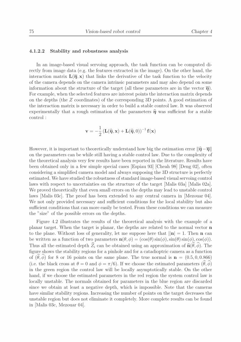
75 Vision-based robot control Chapter 4
4.1.2.2 Stability and robustness analysis
In an image-based visual servoing approach, the task function can be computed di-rectly from image data (e.g. the features extracted in the image). On the other hand, theinteraction matrix L(η,x) that links the derivative of the task function to the velocityof the camera depends on the camera intrinsic parameters and may also depend on someinformation about the structure of the target (all these parameters are in the vector η).For example, when the selected features are interest points the interaction matrix dependson the depths (the Z coordinates) of the corresponding 3D points. A good estimation ofthe interaction matrix is necessary in order to build a stable control law. It was observedexperimentally that a rough estimation of the parameters η was sufficient for a stablecontrol :
v = −1
2(L(η,x) + L(η, 0))−1 f(x)
However, it is important to theoretically understand how big the estimation error ‖η−η‖on the parameters can be while still having a stable control law. Due to the complexity ofthe theoretical analysis very few results have been reported in the literature. Results havebeen obtained only in a few simple special cases [Espiau 93] [Cheah 98] [Deng 02], oftenconsidering a simplified camera model and always supposing the 3D structure is perfectlyestimated. We have studied the robustness of standard image-based visual servoing controllaws with respect to uncertainties on the structure of the target [Malis 03a] [Malis 02a].We proved theoretically that even small errors on the depths may lead to unstable controllaws [Malis 03c]. The proof has been extended to any central camera in [Mezouar 04].We not only provided necessary and sufficient conditions for the local stability but alsosufficient conditions that can more easily be tested. From these conditions we can measurethe ”size” of the possible errors on the depths.
Figure 4.2 illustrates the results of the theoretical analysis with the example of aplanar target. When the target is planar, the depths are related to the normal vector nto the plane. Without loss of generality, let me suppose here that ||n| = 1. Then n canbe written as a function of two parameters n(θ, φ) = (cos(θ) sin(φ), sin(θ) sin(φ), cos(φ)).
Thus all the estimated depth Zi can be obtained using an approximation of n(θ, φ). Thefigure shows the stability regions for a pinhole and for a catadioptric camera as a functionof (θ, φ) for 8 or 16 points on the same plane. The true normal is n = (0.5, 0, 0.866)
(i.e. the black cross at θ = 0 and φ = π/6). If we choose the estimated parameters (θ, φ)in the green region the control law will be locally asymptotically stable. On the otherhand, if we choose the estimated parameters in the red region the system control law islocally unstable. The normals obtained for parameters in the blue region are discardedsince we obtain at least a negative depth, which is impossible. Note that the camerashave similar stability regions. Increasing the number of points on the target decreases theunstable region but does not eliminate it completely. More complete results can be foundin [Malis 03c, Mezouar 04].

Ezio Malis 76
θ
φ−90 −60 −30 0 30 60 90
−90
−60
−30
0
30
60
90
θ
φ−90 −60 −30 0 30 60 90
−90
−60
−30
0
30
60
90
Pinhole camera (8 points) Pinhole camera (16 points)
θ
φ−90 −60 −30 0 30 60 90
−90
−60
−30
0
30
60
90
θ
φ−90 −60 −30 0 30 60 90
−90
−60
−30
0
30
60
90
Catadioptric camera (8 points) Catadioptric camera (16 points)
Fig. 4.2 – Stability regions for planar targets with 8 or 16 points observed by a pinholeor a catadioptric camera. Parameters (φ, θ) selected in the green regions lead to stablecontrol while parameters selected in the red regions lead to unstable control.
4.2 Design of robust visual servoing schemes
Despite the improvements in the design of image-based control laws, the theoreticalanalysis of the robustness shows that for the considered control laws we need an estimationof the structure of the target. Therefore, it is important to investigate control methodsthat do not explicitly need this estimation.
4.2.1 Increasing the robustness of image-based approaches
4.2.1.1 A new class of visual servoing schemes
In [Malis 02f] we proposed a new class of visual servoing schemes that encompassesseveral image-based visual servoing approaches such as [Malis 99, Basri 99]. The newclass of visual servoing schemes is based on the reconstruction of the pose (up to a scalefactor for the translation) of the camera from two images. The key idea of the new class

77 Vision-based robot control Chapter 4
is to estimate the rotation from two views. Therefore the rotation is directly controlledand decoupled from the control of the translation. The translation can be controlled inseveral different ways which differentiate between the possible methods within the class.This class of methods has interesting properties. Since the rotation control is decoupledfrom the translation control, it is possible to ”easily” study the stability and robustnessof the control law with respect to errors on the intrinsic and extrinsic camera parameters(the extrinsic parameters are the pose of the camera with respect to the robot end-effector) [Malis 01a, Malis 02f]. Again, the analysis of the robustness of the control lawis very important since it allowed us to show that the ”size”of the calibration error thatthe control laws can tolerate is very large.
The new class of visual servoing schemes is based on the assumption that we canestimate the rotation matrix directly from the current and reference images. In the moregeneral case (i.e. both for non-planar and planar objects), the rotation can be extractedfrom the homography matrix (see Chapter 3). Theoretically, the homography matrix canbe estimated from any sufficient visual information (e.g. a set of points, of lines, ...). Forexample, we proposed in [Chesi 00] a complete vision-based control system with respectto planar contours. In the system we integrated the visual matching [Chesi 99], the visualtracking [Drummond 99] and the visual servoing [Malis 99]. However, this integrationwork highlighted two problems in our approach. First of all, the feature-based estimationfor the task function was specific to planar contours. A different system should be built fordifferent features. Secondly, it is impossible to compute the rotation from the homographymatrix using image data only (the current and reference image). Indeed, there are twopossible solutions when we decompose an homography matrix. This second problem ledus to propose a different vision-based control method that is detailed in the next section.
The solution to the first problem has been to estimate the homography directly fromimage data without any feature extraction [Malis 04d, Malis 05]. We use the ESM forthe direct image registration of a planar surface (see Section 3). This allowed us tosimplify the design of the visual servoing approach and to increase its flexibility sincethe planar surface can contain any information. Figures 4.3 and 4.4 show a vision-basedcar-platooning experiment that is performed in a real outdoor environment.
Figure 4.3 gives an overview of the system while Figure 4.4 illustrates more detailsof the experiment. Two electric vehicles of type ”Cycab” are used : one as a guider carand the other as a follower car. A driver guides the first car while the follower car iscontrolled by a position-based control scheme. The control scheme takes into accountthat the vehicle is non-holonomic and tries to keep the distance between the two vehiclesconstant and equal to the initial distance. The relative position is given by the ESMvisual tracking system. The pan-tilt turret is controlled in order to keep the guider carin the field of view of the camera during the experiment.

Ezio Malis 78
In the starting situation, when the guider car is in front of the follower car, a windowof (100×100) pixels is selected to be the reference pattern. In order to have a metricreconstruction, the camera was roughly calibrated and the distance between the two carsis given to the control process. It is the distance between the camera of the follower carand a poster stacked on the back windshield of the guider car. Tracking this referencepattern provides the relative position between the two vehicles. The blue square indicatesthe tracked region. In the right column, the reprojections of the tracked region usingthe estimated homographies are shown. The first row of the figure corresponds to theinitial position. The ESM tracking algorithm performs well although the experimenttakes place outdoors and sun reflection on the tracked region occurs. The current patternreprojections are very close to the reference one. More details on the experiment can befound in [Benhimane 05].
Low−level wheel steering controlLow level velocity control
CAN bus controller
Wheel steering controlVelocity control
Serial comm. RS232
Tracking SoftwareESM Vision
Frame grabber
Pan−Tilt turretCCD Camera
Computer 2 − Pentium III 700 MHz Computer 1 − Pentium III 700 MHz
CAN bus comm. process
TCP/IP socket comm. process
Fig. 4.3 – Overview of the compete system.

79 Vision-based robot control Chapter 4
Fig. 4.4 – Several images of a platooning application. The first column shows the redcar automatically following the leader. The second column shows the area of interest inthe current image. The third column shows the registered images that prove that thehomography has been correctly estimated.
Ezio Malis 80
4.2.1.2 Direct visual servoing
As already mentioned, our objectives have been to find a task function that is dif-feomorphic to the pose of the camera and to find a stable control law that can easilybe computed just from visual data extracted from the current and the reference images(independently of the shape of the object). If the target is not planar these objectives canbe fulfilled by the visual servoing schemes presented in the previous section. On the otherhand, when the target is planar, image data from the reference and current image onlyis not sufficient to compute the control law. In this case, the two images of the target arerelated by a homography matrix. The decomposition of the homography generally hastwo solutions and we need additional information to distinguish the true solution fromthe false one.
Therefore, we studied how the two solution of the decomposition are related (seeChapter 3). In [Vargas 05] we proved that the two solution of the homography can be”mixed” in the computation of a stable control law. For example, we defined a taskfunction containing the average of the two translations and of the two rotations (on theSO(3) group). Alternatively we can compute the average of the two rotations and controlthe remaining d.o.f.s as for the 2.5D visual servoing [Malis 07b]. With such an approachwe can completely avoid the use of ”a priori” information to choose the true solution ofthe homography decomposition. However, contrary to the 2.5D visual servoing schemethe stability analysis becomes extremely difficult since the rotation control is no longerdecoupled from the translation control.
In [Benhimane 06a] we proposed a task function that is locally diffeomorphic to thecamera pose and that can be directly computed from the homography matrix. Therefore,we completely avoid the decomposition process. We also proposed a simple control law andwe theoretically proved its local stability. Experimentally we observed that the stabilityregion is very large (see the experiments below). In order to build a globally stable controlscheme we should plan a trajectory and work with small errors. This was not possible withthe task function proposed in [Benhimane 06a] since it was only locally diffeomorphic tothe camera pose. Another limitation of the approach was that it was designed for planartargets only.
Recently, we have generalized the approach to non-planar targets and we have modifiedthe task function to allow for path planning [Silveira 07a]. We have also proposed a simplecontrol law and we have theoretically prove its local stability. The general task functionthat we have proposed is the following :
ε =
[(H − I)q + ρ t
ϑ(H)µ(H)
](4.1)
where H is a homography matrix related to a virtual plane, t is the translation, q is achosen control point in the reference image that corresponds to a point on the target,and ρ is a scalar that encodes the parallax of this point with respect to the virtualplane. Finally, [µ(H)]
×= H − H⊤ and ϑ(H) is detailed in [Silveira 07a]. Note that the
task function can be computed from image data only (i.e. we do not measure t and ρseparately but the vector ρ t, which is measured from the epipolar geometry). This task

81 Vision-based robot control Chapter 4
function generalizes the one proposed in [Benhimane 06a] for planar targets. Indeed, forplanar targets the parallax is zero ρ = 0 and if we set ϑ(H) = 1 we obtain the sametask function proposed in [Benhimane 06a]. The modification that allows us to performtrajectory planning is on the scale factor ϑ(H) (see [Silveira 07a]).
The experimental validation of the direct visual servoing approach is in progress. I willdescribe here two experiments for the planar case [Benhimane 06a] and two promisingsimulations for the general case [Silveira 07a].
We have tested the control scheme proposed in [Benhimane 06a] on the Cartesianrobot of the LAGADIC research team at INRIA Rennes. The robot is accurately calibra-ted and it provides a ground truth for measuring the accuracy of the positioning task.A calibrated camera is mounted on the end-effector of the robot and observes a planartarget. Starting from another pose (the initial pose) which allows the target to be seenfrom a different view point, the robot is controlled using the control law in order to getback to the reference pose. At the initial pose the translation displacement is 0.68 metersand the rotation displacement is 96 degrees. We use the ESM visual tracking algorithm[Benhimane 04] to register the area of interest and to estimate at the same time an un-calibrated homography matrix G. We use the center of gravity of the template as thecontrol point.
In the first experiment, illustrated in Figure 4.5, we used the true camera intrinsicparameters matrix K to obtain a calibrated homography H = K−1GK from which thecontrol law is computed. The control law is stable and both translation and rotationvelocities converge to zero. At the convergence, the robot is back to its reference poseand the visual information coincides with the visual information of the reference pose.As shown in Figure 4.5, the camera displacement converges to zero very accurately (lessthan 1 mm error for the translation and less than 0.1 degrees for the rotation).
Figure 4.6 illustrates a second experiment that is performed under similar conditions(the same initial camera displacement, an unknown normal vector to the plane, an unk-nown camera/object distance...). On the other hand, we use a very bad estimation of
the camera intrinsic parameters to estimate the homography matrix H = K−1GK. Ho-wever, the control law is robust to camera calibration errors : the translation and therotation velocities converge to zero. At the convergence, the visual information coincidesagain with the visual information of the reference image and the camera displacementconverges to zero (as in the previous experiment we obtain around 1 mm error for thetranslation and around 0.1 degrees for the rotation).
We have performed two simulations to validate the general control scheme proposedin [Silveira 07a]. We used the image registration algorithm proposed in [Malis 07a] tomeasure an uncalibrated homography G and the vector ρ e from which we obtainedH = K−1 GK and ρ t = ρ K−1e.
The first simulation in Figure 4.7 shows that the new control scheme encompasses theprevious one specifically designed for planar targets. Additional simulations can be foundin [Silveira 07a] that show how path planning can handle larger initial displacements thanthe previous approach.
The second simulation in Figure 4.8 shows that the general control scheme workswell with non-planar targets and for very large displacements. We planned a straight line

Ezio Malis 82
trajectory in the image for the control point in order to keep the target in the field of viewof the camera. In this simulation we also added errors in the estimated camera intrinsicparameters in order to demonstrate the robustness of the control law.
Reference image Initial image Final image
0 200 400 600 800−0.02
−0.01
0
0.01
0.02
0.03
0.04
0.05ν
x
νy
νz
0 200 400 600 800−10
−8
−6
−4
−2
0
2
4
ωx
ωy
ωz
Translation velocity Rotation velocity
0 200 400 600 800−0.8
−0.7
−0.6
−0.5
−0.4
−0.3
−0.2
−0.1
0
0.1
0.2
tx
ty
tz
0 200 400 600 800−20
0
20
40
60
80
100rx
ry
rz
Translation error Rotation error
Fig. 4.5 – Direct visual servoing with respect to a planar target. A calibrated pinholecamera is mounted on a calibrated Cartesian robot.

83 Vision-based robot control Chapter 4
Reference image Initial image Final image
0 200 400 600 800 1000−0.02
−0.01
0
0.01
0.02
0.03
0.04
0.05
νx
νy
νz
0 200 400 600 800 1000−10
−8
−6
−4
−2
0
2
4ω
x
ωy
ωz
Translation velocity Rotation velocity
0 200 400 600 800 1000−0.8
−0.7
−0.6
−0.5
−0.4
−0.3
−0.2
−0.1
0
0.1
0.2
tx
ty
tz
0 200 400 600 800 1000−20
0
20
40
60
80
100rx
ry
rz
Translation error Rotation error
Fig. 4.6 – Direct visual servoing with respect to a planar target. An uncalibrated pinholecamera is mounted on a calibrated Cartesian robot.
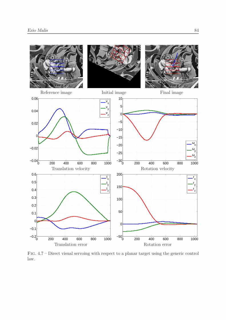
Ezio Malis 84
Reference image Initial image Final image
0 200 400 600 800 1000−0.04
−0.02
0
0.02
0.04
0.06
vx
vy
vz
0 200 400 600 800 1000−30
−25
−20
−15
−10
−5
0
5
10
ωx
ωy
ωz
Translation velocity Rotation velocity
0 200 400 600 800 1000−0.2
−0.1
0
0.1
0.2
0.3
0.4
0.5
0.6
txtytz
0 200 400 600 800 1000−50
0
50
100
150
200
rx
ry
rz
Translation error Rotation error
Fig. 4.7 – Direct visual servoing with respect to a planar target using the generic controllaw.

85 Vision-based robot control Chapter 4
Reference image Initial image Final image
0 50 100 150−0.2
−0.1
0
0.1
0.2
0.3
vx
vy
vz
0 50 100 150−30
−25
−20
−15
−10
−5
0
5
10
ωx
ωy
ωz
Translation velocity Rotation velocity
0 50 100 150
−0.6
−0.4
−0.2
0
0.2
0.4
txtytz
0 50 100 150−20
−10
0
10
20
30
40
rx
ry
rz
Translation error Rotation error
Fig. 4.8 – Direct visual servoing with respect to a non-planar target using an uncalibratedpinhole camera

Ezio Malis 86
4.2.2 Beyond standard vision-based control approaches
Standard vision-based control approaches have been widely studied and several suc-cessful applications have been performed. One may wonder if it is possible to go beyondthe assumption behind these standard approaches. That is, can we achieve a task with animage-based approach despite the fact that the imaging conditions have changed ? Howcan we achieve a task using a monocular vision system with a position-based approachdespite the fact that a metric model of the scene is unknown ? The following sectiondescribes two possible answers to these questions.
4.2.2.1 Visual servoing invariant to camera intrinsic parameters
The main assumption of the teaching-by-showing approach is that a reference imagehas been acquired and that the imaging conditions do not change. I proposed in [Malis 04b]to eliminate this assumption in order to enlarge the domain of application of the teaching-by-showing approach. More precisely, I showed that for pinhole cameras it is possible todefine an error from image data that does not depend on camera intrinsic parameters.The error only depend on the pose of the camera with respect to the target. The inva-riant error can be defined for several types of visual features like points, lines, contours[Malis 01c, Malis 02e].
Consider for example that the camera observes n > 3 non-colinear points. The imagehomogeneous coordinates p
ijdepend on the camera internal parameters Ki and on the
homogeneous normalized coordinates qij
:
pij
= Ki qij(4.2)
We can define two positive symmetric matrices Sq and Sp as follows :
Sq =1
n
n∑
j=1
qijq⊤
ij= MqM
⊤
q and Sp =1
n
n∑
j=1
pijp⊤
ij= Mp M⊤
p
where Mq and Mp are upper triangular matrices obtained applying the Cholesky decom-position to Sq and Sp respectively. The two matrices are related by :
Mp = KiMq (4.3)
Thus, it is possible to compute the invariant vectors iij with the following transformation :
iij = M−1p p
ij(4.4)
Note that the vectors iij are computed only from the image coordinates. Using equa-tions (4.3) and (4.2), we can prove that the vectors iij only depends on the normalizedcoordinates q
ij:
iij = M−1p p
ij= M−1
q K−1i Ki qij
= M−1q q
ij(4.5)
As a consequence, the vectors iij are independent of the camera intrinsic parameters Ki.

87 Vision-based robot control Chapter 4
The transformation of the image points in the invariant space can be performedboth for the reference image and the current image. In order to regulate the error tozero, I proposed a vision-based control technique based on the task function approach[Malis 01b, Malis 04b]. Another interesting property of the visual servoing invariant tocamera intrinsic parameters is that it is possible to define trajectories in the invariantspace such that the camera trajectory is a straight line in the Cartesian space [Malis 02d].
Figure 4.9 shows an example of invariant visual servoing performed with the calibratedCartesian robot of the Lagadic research team at INRIA Rennes. The reference image isacquired with a 12 mm lens while a 6mm lens is used for servoing. The images in thelast row of the figure show that the errors on the translation and the rotation of theend-effector converge to zero. If we look at the trajectory of the points in the image wecan note that the final image (the green points) is obviously different from the referenceimage (the yellow points). On the other hand, the error on the coordinates of the pointsin the invariant space converge to zero.
Visual servoing with zooming cameras
An obvious extension of the invariant visual servoing approach was to show that thecamera intrinsic parameters may vary during the servoing [Malis 02e]. Moreover, it ispossible to define a method [Malis 02c] that unifies model-based approaches and image-based approaches. Since the error does not depend on the camera intrinsic parameters,a zooming camera can be used in order to keep the target in the camera field of view(zoom out) or to obtain a better resolution (zoom in) [Benhimane 03]. In this case it ispossible to have two separate control laws for positioning the camera and for zooming.This approach allows the domain of applicability of visual servoing to be enlarged.
Indeed, being able to zoom out on the target can reduce visibility problems. Howe-ver, when we zoom in to increase the resolution some features may disappear and otherfeatures may become visible. The appearance/disappearance of the visual informationduring the servoing produces discontinuities in the control law that perturb the perfor-mances of the system. Indeed, when one or several features appear or disappear duringthe servoing they are added to or deleted from the task function. The amplitude of thediscontinuity depends on : i) the number of visual features, ii) the error in the image, iii)the conditioning of the interaction matrix. In [Garcia-Aracil 05a], we proposed a solutionto avoid the discontinuities by giving a weight to each feature. We applied this approachto the invariant visual servoing [Garcia 04a], [Garcia-Aracil 05b], [Garcia 04b], but theapproach can also be extended to standard image-based approaches.
3D Reconstruction with invariant active stereo-vision
The invariant visual servoing scheme has been used to develop an active vision methodin order to improve the 3D reconstruction of natural 3D objects in the sea. We usea stereo pair mounted on a robot manipulator that lies on the ground. We constrainthe displacements of the stereo pair by repeating the invariant visual servoing (the twocameras do not have the same intrinsic parameters) of the left camera on the right one

Ezio Malis 88
several times [Brandou 06]. Thus, the geometry of the stereo pair define the trajectoryfollowed by the cameras. This simplifies the reconstruction process (constraint trajectory,reduction of the unknowns [Brandou 07]. We have also shown that the reconstructionprocess can be done in the invariant space reducing the number of unknowns of thebundle adjustment problem [Malis 04c].
Reference image Initial image
0 50 100 150 200 250 300 350
0
50
100
150
200
250
1 2
3 4 5
6
7
8
9 10
11 12
1
2
3
4
5
6
7
8
9
10
11
12
50 100 150 200 250 300 350 4000
0.05
0.1
0.15
0.2
0.25
0.3
iterations number
||dq|
|
error in the invariant space
50 100 150 200 250 300 350 400
−0.1
0
0.1
0.2
0.3
iterations number
t
translation error
txtytz
50 100 150 200 250 300 350 400−80
−60
−40
−20
0
20
40
iterations number
uθ
rotation error
ux θ
uy θ
uz θ
Fig. 4.9 – Intrinsics-free visual servoing using a 12mm lens for learning the referenceimage and a 6mm lens during the servoing.

89 Vision-based robot control Chapter 4
4.2.2.2 Controlled visual simultaneous localization and mapping
In the standard ”position-based” visual servoing approaches the reference pose withrespect to a known target is directly given by the user [Wilson 96, Martinet 97]. Therefore,we need the model of the scene to compute the pose. We have extended this concept tovisual servoing tasks when the model of the scene is not (completely) known [Silveira 06b].Like standard ”position-based” visual servoing approaches, the robot is directly controlledin the Cartesian space with a standard control law. However, the idea behind our approachis to perform a controlled visual SLAM. Indeed, the reference pose may be located veryfar away from the initial pose such that the same part of the scene may not always bemaintained in the camera field of view as illustrated in Figure 4.10. Thus, newly observedparts of the rigid scene must be integrated into the scheme. The proposed approach isadapted to robot navigation in large environments.
������������
������������������
������
���������
���������
����������
����������
�������������������������������������������������������
�������������������������������������������������������
��������������������
��������������������
����������
����������
������������������������������������������������������������
������������������������������������������������������������
1Tk
0T1
Ik
I1
I0
Fig. 4.10 – Controlled visual simultaneous localization and mapping.
The applicability of such an approach depends on the accuracy of the visual SLAMestimation. Since the task is uniquely defined in terms of a pose to be reached, smallcalibration and measurement errors may produce gross errors after long distances. Thechallenge is thus to obtain very precise estimations of structure and motion. We use ourdirect visual SLAM approach described in Section 3 to simultaneously estimate the struc-ture and camera localization [Silveira 07c]. In order to speed up the on-line estimationwe can suppose the scene is piecewise planar and we can detect the part of the scene thatbest fits our model. When a new part of the scene appears in the image the new planarregions are automatically detected [Silveira 06a]. Ath the time of writing, the experimen-tal validation of the approach is in progress. However, promising simulation results can

Ezio Malis 90
be found in [Silveira 06b].

Conclusion and future research
When dealing with real-time robotic applications, it is important to take into accountvery early at the design level the respective specificities and requirements of vision-basedestimation and vision-based control problems. By doing so, we have not only improvedthe performances during the execution of a task but also proposed methods and algo-rithms that perform better than approaches that consider vision-based estimation andvision-based control problems separately.
One important contribution has been to propose the Efficient Second-order approxi-mation Method (ESM) for solving non-linear systems of equations defined on Lie Groupswhen additional information on the derivatives at the solution can be measured. Indeed,the ESM has been successfully applied both to vision-based estimation and to vision-basedcontrol. The theoretical results predict a higher convergence rate and a larger convergencedomain with respect to standard numerical methods. These theoretical results have beenconfirmed by several experiments.
Another contribution has been the design of direct methods for image registration.This has permitted the accurate and robust estimation of structure and/or motion inlarge scale environments, despite occlusions and large changes in the illumination condi-tions. The proposed approach is generic, it can be used with any central catadioptriccamera and it naturally extends to stereo-vision systems. The effective application of theESM to our approach supposes that the Jacobians can be measured from image dataonly. We have shown when and how this can be possible using Lie groups theory. Wehave also experimentally shown that the ESM has very good performances even whenthe Jacobians are only approximated.
Various contributions have been made to the design of vision-based control schemes.We showed that standard image-based visual servoing schemes can be improved by usingthe ESM to design the control law. Theoretical stability and robustness analysis haveallowed bounds on the “size” of the possible calibration errors to be found. Then, severalcontributions have been made to the design of robust vision-based control schemes thatdo not need an exact measure of the parameters of the vision system and that do notneed any “a priori” knowledge of the structure of the observed scene. Again, a particularemphasis has been placed on the theoretical analysis of the robustness of the controllaws with respect to errors on the parameters. Finally, we have proposed methods that

Ezio Malis 92
go beyond the teaching by showing approach. We have shown how to define an errorfunction for pinhole cameras that is invariant to camera intrinsic parameters. This allowsus to define new tasks using zooming cameras. Another new promising approach is tointegrate vision-based control into simultaneous localization and mapping approaches.
Future Research
In my future research work, I intend to develop a low level vision framework as gene-ric as possible and well adapted to robotic applications. This framework must be able toaddress a large number of situations frequently met : different sorts of cameras (centralor not), large illumination changes, rigid/deformable objects, static/dynamic scenes, etc.The low level vision framework should also be generic enough to be coupled with otherinteroceptive and/or exteroceptive sensor information in order to obtain a reliable androbust localization for robotic applications. I believe that one way to achieve these objec-tives is to further study and develop direct methods. Within this framework, three mainproblems must be addressed.
The first problem is to find simple, accurate, yet general models of the plenopticfunction. In particular, we need general photometric models, general camera models andgeneral structure models. General photometric models should be able to take into accountnot only illumination changes but also colorimetric information. General camera modelsshould be able to take into account non-central projection cameras. General structuremodels should be able to take into account not only complex rigid environments butalso unknown deformable environments. These models should be realistic, but not overlycomplex in order to comply with computational real-time requirements of robotic applica-tions. Finding the right compromise is a delicate and difficult issue. Indeed, the qualitiesof a model depend on the problem for which it is used (simulation, estimation, control),and a solid methodology (which could guide the choices in this respect) does not exist.
The second problem is the efficient estimation of the parameters associated with themodels. The optimization techniques efficient enough for real-time robotic tasks have onlylocal convergence. Thus, a fairly accurate initialization is needed (i.e. an estimate of thetrue unknown parameters). We can study how to efficiently initialize the local optimi-zation schemes using fast data association algorithms or relying on external information(complementary sensor modalities). However, a more general and elegant solution wouldbe the study of efficient global optimization methods. For example, I am currently in-vestigating if and how the use of Interval Analysis as a global optimization tool can becompatible with real-time constraints. With respect to other global optimization tech-niques, the main advantage of Interval Analysis is that the solutions to the problem canbe certified.
The third problem is the use of complementary sensor modalities and fusion tech-niques. This allows the localization and mapping tasks to be simplified and robustified

93 Conclusion and future research
when dealing with large scale environments. For example, a typical multi-sensor systemis composed of one or more vision sensors and/or a range sensor (laser or radar) withthe complement of an absolute positioning sensor (e.g. an inertial navigation system or aglobal navigation system). To cope with multi-sensor data, I intend to relies on the directapproach for each sensor, and to study appropriate filtering techniques in order to takeinto account the uncertainty of each sensor.
Another objective of my future research work will be to further investigate the directvision-based robot control approach. The design of standard vision-based control schemesrely on several assumptions : on the geometric and photometric properties of the environ-ment, on the characteristics of the imaging device and on the characteristic of the robot.My objective is to increase the precision and the robustness of direct vision-based controlalgorithms despite modeling errors induced by these assumptions. On the one hand, Iwill investigate the design of control algorithms that are robust with respect to noise andmodeling errors and analyze the associated robustness properties. On the other hand,I will study the connections between the design of robust control laws and the systemmodeling, with the objective of investigating if and how the assumptions on the geome-tric and photometric properties of the environment, on the characteristics of the imagingdevice and of the robot can be relaxed. A key point will be to handle the compromisebetween the complexity of the models, the real time aspects and the robustness of thecontrol algorithms.
Concerning the assumptions on the vision system there are three assumptions thatwe should relax. The first assumption to be relaxed should be the use of central cameras.Indeed, non-central cameras can be useful in many applications since some of them haveconstant resolution. To my knowledge, the use of non-central cameras for direct vision-based control has not yet been investigated. A second assumption to be relaxed should bethe rigidity of the environment. Thus, I will investigate whether control methods whichdo not involve an explicit metric reconstruction of a model of the environment and havebeen proposed for rigid objects, can be applied to deformable ones. The key problem isthe characterization of a diffeomorphism between the sensory information and the pose ofthe robot. The third assumption is that the environment is Lambertian. This assumptionis obviously not verified in practice and the estimation of the position of the light sourcesin the environment can be used to increase the accuracy and robustness. Note that thisinformation can also be taken into account in the design of the control law in order toavoid the presence of specular reflection or shadows in the image.
Concerning the assumption on the characteristic of the robot, I have considered sofar vision-based control applied to holonomic mechanisms. The control of these systemsis much simpler due to the fact that instantaneous motion along any direction of theconfiguration space is possible. A consequence of this is that generic vision-based controllaws can be designed independently of the mechanism specificity. However, this is nottrue in the case of critical systems like most ground, marine or aerial robots. I haveproposed control schemes for holonomic robots whose performance does not depend on

Ezio Malis 94
parameters that cannot easily be estimated on-line (e.g. camera intrinsic parameters, poseand 3D parameters of the target). Such control laws are structurally robust with respectto estimation errors on the parameters. I plan to study whether these techniques can begeneralized to critical nonlinear systems.

Appendix : Resume en francais
Introduction
La conception de systemes robotiques completement autonomes est une des grandesambitions de l’humanite. De nos jours des progres theoriques et technologiques ont permisaux ingenieurs de concevoir des systemes robotiques complexes qui peuvent remplacer lesetres humains dans de nombreuses applications qui peuvent etre repetitives ou dange-reuses. Toutefois, afin d’etendre la flexibilite et le domaine d’application de ces systemesautonomes, nous devons encore resoudre plusieurs problemes scientifiques qui sont a lacroisee de plusieurs domaines tel que l’intelligence artificielle, le traitement du signal etla theorie de la commande.
Parmi ces defis scientifiques, la perception de l’environnement et l’interaction d’unsysteme robotique avec son environnement sont des problemes fondamentaux dans laconception de tels systemes autonomes. En effet, les performances d’un robot autonomedependent non seulement de la precision, de la continuite et de la fiabilite de sa perceptionmais aussi de son habilite a utiliser l’information percue dans des boucles de commandeafin d’interagir de maniere sure avec son environnement malgre les inevitables erreurs demodelisation et de mesure. Pour ces raisons, la modelisation et la perception de l’envi-ronnement et la commande referencee capteur robuste sont des problemes scientifiquesmajeurs en robotique.
Plusieurs capteurs exteroceptifs sont couramment utilises en robotique : GPS, cap-teurs optiques, capteurs de contacts, sonars, telemetres lasers, et meme des capteurs audi-tifs et olfactifs. Toutefois, la vision artificielle a un interet et une importance particuliereprincipalement due a sa versatilite. Elle peut etre utilisee a la fois pour la modelisation etla perception et pour la commande du robot. Dans ce contexte, l’etendue des recherchesest tres vaste et je focaliserai ce document sur l’estimation et la commande a partir d’unsysteme de vision. L’estimation a partir de la vision concerne des methodes dediees al’extraction des informations qui peuvent etre utilisees a la fois pour la modelisation del’environnement et pour la commande des robots. Dans le cas des applications robotiques,les defis majeurs sont d’augmenter l’efficacite, la precision et la robustesse de l’estimationa partir des donnees capteurs. La commande referencee vision concerne des methodesdediees a l’utilisation des informations visuelles dans des boucles de commande. Les defissont le choix approprie de l’information et la conception de lois de commande stables etrobustes aux erreurs de modelisation et de mesure.

Ezio Malis 96
L’objectif de ce document est de resumer, analyser et discuter mes travaux de re-cherche sur ces sujets pendant les derniers dix annees : deux ans comme Research As-sociate a l’Universite de Cambridge (Grande Bretagne) et huit ans comme Charge deRecherche a l’INRIA Sophia-Antipolis (France). Afin de reconnaıtre les contributionsde tous les collegues et les etudiants avec lesquels j’ai collabore, j’ai essaye autant quepossible de citer toutes nos publications en commun.
Activites de recherche
Mes activites de recherche se situent a la croisee de la vision par ordinateur et dela commande referencee capteurs des systemes dynamiques. La principale problematiqueabordee dans mes travaux est comment utiliser les informations capteur dans des bouclesde commande afin de rendre un robot le plus autonome possible dans la realisation destaches de type reflexe.
Pendant mon travail de post-doctorat, qui a ete effectue a l’Universite de Cambridgedans le cadre du projet europeen VIGOR, j’ai tout d’abord generalise une partie de mestravaux de these a une nouvelle classe de methodes d’asservissement visuel. Ensuite, j’aiapporte une solution au probleme de la robustesse des lois de commande lie aux erreursd’etalonnage de la camera. Enfin, j’ai traite le probleme de la conception d’un systemecomplet de commande referencee vision.
Une nouvelle classe de methodes d’asservissement visuel
Une partie tres importante de mon travail de post-doctorat a ete de montrer quela methode d’asservissement visuel proposee dans ma these est un cas particulier d’uneclasse plus large de schemas d’asservissement visuel [Malis 02f]. Par exemple, dans lameme classe on peut concevoir un schema d’asservissement de type “asservissement visuel3D” en definissant comme fonction de tache une erreur sur l’attitude de la camera. Cettenouvelle classe possede des proprietes tres interessantes. En particulier, il est possibled’effectuer une analyse formelle de la stabilite et de la robustesse par rapport aux pa-rametres intrinseques et extrinseques de la camera (le parametres extrinseques definissentl’attitude de la camera par rapport a l’effecteur du robot) [Malis 01a]. L’importance del’analyse de la robustesse reside dans la connaissance du taux d’erreur d’etalonnage quele systeme peut supporter.
Auto etalonnage des cameras
Bien que la loi de commande proposee s’avere assez robuste, si les erreurs d’etalonnagesont tres grands le systeme peut avoir des performances reduites et il peut meme devenirinstable. Une solution classique est de bien etalonner la camera prealablement. Cetteetape est importante mais elle est souvent difficile a mettre en oeuvre et peu flexible.La deuxieme possibilite, plus flexible, est d’auto etalonner la camera en ligne. Dans ce

97 Activites de recherche
contexte, ma contribution principale a ete de formuler le probleme de l’auto etalonnagea partir d’objets planaires d’une maniere tres intuitive du point de vue geometrique[Malis 02g]. L’auto etalonnage est obtenu en imposant la contrainte que la scene observeeest rigide. Donc, la normale au plan dans un repere fixe est constante quelque soit le pointde vue [Malis 00b]. L’interet de l’auto etalonnage est que, sous certaines conditions, onpeut estimer la distance focale de la camera meme si elle change au cours du temps[Malis 00c].
Conception d’un systeme de commande referencee vision
Un systeme complet d’asservissement visuel ne se reduit pas au choix de la fonctiond’erreur a reguler et a la conception de la loi de commande mais doit tenir compte aussid’un systeme de mesure de l’erreur [Malis 03b]. En collaboration avec G. Chesi nousavons propose un systeme complet pour la commande referencee vision par rapport a descontours plans. Dans ce systeme, nous avons integre l’association des donnees (mise encorrespondance et suivi) et la commande [Chesi 00]. La mise en correspondance consistea localiser dans deux images les projections d’un meme pont de la scene. Notre contribu-tion a ete de proposer un algorithme pour la mise en correspondance de contours plans[Chesi 99]. Ce travail d’integration est tres important pour la suite de mes recherches caril a mis en evidence les limites des approches classiques de conception des systemes decommande referencee vision (qu’on peut classifier comme “reductionnistes”). La loi decommande utilisee n’etait pas assez generique car elle necessite une connaissance sur lanormale au plan. De plus, le systeme de mesure etait specifique a des contours plan etdifficilement reutilisable dans d’autres applications.
A la suite de mon recrutement a l’INRIA en Octobre 2000 j’ai poursuivi mes travaux derecherche sur la commande referencee vision. Tout d’abord, afin d’augmenter la robustesseet la flexibilite des methodes de type “asservissement visuel 2D”, j’ai travaille sur laconception des nouvelles methodes d’asservissement et sur la vision active. Ensuite j’aitravaille sur l’extension du domaine d’application de la commande referencee vision afinde passer des taches de positionnement d’un robot manipulateur aux taches de navigationd’un robot mobile en environnement inconnu. C’est dans ce contexte que me travaux derecherche ont peu a peu evolue vers une approche plus holistique a l’integration desalgorithmes de vision par ordinateur dans les systeme de commande referencee vision.Dans ce cadre, j’ai developpe un nouvel axe de recherche transversal concernant desmethodes d’optimisation efficaces et robustes.
Travaux de recherche en asservissement visuel 2D
Une contribution tres importante de mes travaux a ete de proposer une extensionde l’approche “apprentissage par demonstration” : l’asservissement visuel 2D invariantaux parametres intrinseques de la camera. Mes travaux de recherche sur les methodesd’asservissement visuel 2D ont ete complete par une analyse de la robustesse des loi decommande et une etude sur les problemes de visibilite et de continuite.

Ezio Malis 98
Extension de l’approche “apprentissage par demonstration” : l’asservisse-ment visuel 2D invariant aux parametres intrinseques
En l’absence d’une connaissance metrique complete d’un objet par rapport auquelon veut se positionner, les methodes d’asservissement visuel se basent sur l’apprentissageprealable d’une image de celui ci (l’approche “apprentissage par demonstration”). A partirde cette image l’on extrait des caracteristiques visuelles (point, droites, contours, ...) quiseront utilisees comme amers ”reference” a atteindre dans l’image. A partir d’une positioninitiale differente, le mouvement du robot (et donc de la camera embarquee) est controleafin que les caracteristiques visuelles observees coıncident avec celles de ”reference”. Dansce cas, la camera se trouvera, par rapport a l’objet observe, dans la meme position quecelle de l’apprentissage. De maniere generale, quelque soit la methode d’asservissementvisuel employee, ceci est vrai si et seulement si les parametres intrinseques de la camerasont, a la convergence, les memes que lors de l’apprentissage de l’image de reference. Eneffet, il est evident que si les parametres intrinseques de la camera changent pendantl’asservissement (ou si la camera utilisee pendant l’asservissement n’est pas la memecamera utilisee pendant l’apprentissage), meme si on arrive a atteindre les informationsvisuelles de reference (ce qui n’est generalement pas possible) la position de la camerasera tres differente de sa position a l’apprentissage. Par exemple, si on double la focale,la distance par rapport a un objet doit etre reduite de moitie afin d’observer a peu presla meme image. L’hypothese selon laquelle ”les parametres intrinseques de la camera a laconvergence doivent etre les memes que lors de l’apprentissage de l’image de reference”est tres contraignante.
J’ai donc propose d’eliminer cette contrainte afin d’augmenter considerablement lesdomaines d’application de l’asservissement visuel [Malis 04b]. Plus precisement, j’ai montrequ’il est possible de definir une erreur a partir des donnees image qui ne depende pasdes parametres intrinseques de la camera avec laquelle l’image a ete prise [Malis 01c].Cette erreur ne depend que de la position de la camera par rapport a l’objet observe.Afin de controler le mouvement de la camera et d’asservir cette erreur a zero, j’ai pro-pose une technique d’asservissement visuel 2D basee sur l’approche par fonction de tache[Malis 01b]. L’asservissement visuel invariant aux parametres intrinseques de la cameraest particulierement interessant car il est possible de definir des trajectoires dans l’espaceinvariant sans aucune connaissance des parametres intrinseques. Par exemple, il est pos-sible de definir une trajectoire dans l’espace invariant telle que la trajectoire de la cameradans l’espace cartesien soit une ligne droite [Malis 02d]. La loi de commande qui permetla poursuite de trajectoire est definie directement dans l’espace invariant. Elle doit, au-tant que possible, presenter une grande robustesse aux incertitudes sur les parametresdu systeme et garantir un grand domaine de convergence. Dans le cas de notre nouvelleapproche d’asservissement visuel par rapport aux incertitudes sur la calibration, nousavons montre que le domaine de robustesse est suffisamment grand pour permettre l’uti-lisation d’une approximation grossiere des parametres de calibration tout en conservantla convergence et la stabilite de l’asservissement.
Une extension evidente de l’approche a ete de montrer que les parametres intrinsequesde la camera peuvent varier pendant l’asservissement [Malis 02e]. En plus, il est possible

99 Activites de recherche
de definir une methode [Malis 02c] qui unifie les approches classiques proposees dans lalitterature : celle basee sur la connaissance du modele 3D de l’environnement et cellebasee sur un apprentissage prealable de l’image de reference. De plus, avec cette nouvellemethode il est possible de pallier a un certain nombre de limitations de l’asservissementvisuel classique. Du fait que l’erreur ne depende pas des parametres intrinseques de lacamera avec laquelle l’image a ete prise, le zoom de la camera peut alors etre utilise afinde garder un objet dans l’image (zoom arriere) ou afin d’augmenter sa taille dans l’image(zoom avant) [Benhimane 03]. Dans ce cas, il est possible de separer l’asservissement vi-suel de la camera, de la loi de commande utilisee pour controler le zoom. Cette approchepermet d’augmenter considerablement les domaines d’application de l’asservissement vi-suel.
Analyse de la stabilite et de la robustesse de l’asservissement visuel 2D
Malgre ses propriete d’invariance aux parametres intrinseques de la camera, l’asservis-sement visuel propose appartient a la categorie des methodes dite d’asservissement visuel2D. Dans ce type de methodes la fonction de tache peut etre calculee directement a par-tir des caracteristiques visuelles extraites des images. Toutefois, la matrice d’interactionqui lie la derivee de la fonction de tache a la vitesse de la camera depend de l’informa-tion metrique de l’objet. Une estimation de cette matrice est necessaire afin de concevoirune loi de commande stable. Il a ete observe experimentalement qu’une approximationgrossiere de l’information metrique de l’objet est suffisante pour obtenir une loi de com-mande stable. Toutefois, une question qui n’etait pas resolue est de savoir quelle erreurpeut on commettre sur l’approximation de cette structure tout en garantissant la sta-bilite de la loi de commande. A cause de la difficulte de l’analyse tres peu de resultatstheoriques ont ete obtenus en litterature concernant la stabilite. Cette analyse a pu etreaccomplie seulement pour des simple cas, souvent considerant un modele simplifie decamera, et toujours en supposant que la distribution des profondeurs est estimee parfai-tement. Nous avons etudie la robustesse des methodes d’asservissement 2D par rapportaux incertitudes sur les parametres de la structure [Malis 03a] [Malis 02a]. Nous avonsprouve theoriquement que meme des erreurs relativement petites sur les parametres 3Dpeuvent rendre les lois de commande instables [Malis 03c]. La preuve a ete etendue an’importe quelle camera a centre de projection unique dans [Mezouar 04].
Visibilite et continuite de l’asservissement visuel 2D
Dans l’asservissement visuel 2D les informations extraites des images courante et dereference sont “combinees” dans une fonction de tache qui a la meme dimension quel’espace des configurations du robot (6. d.d.l. pour un robot manipulateur). Toutefoisde nombreuses informations visuelles peuvent ne plus etre disponibles pendant la tache(occultation, sortie de l’image, etc..) et l’etre a nouveau apres un certain delai. La dis-parition/apparition d’informations visuelles pendant l’asservissement produit des discon-tinuites dans la loi de commande qui perturbent les performances du systeme. En effet,quand une ou plusieurs informations disparaissent ou apparaissent pendant l’asservisse-ment elles sont enlevees ou ajoutees de la fonction de tache. Ceci produit une disconti-nuite dans la loi de commande. L’amplitude de cette discontinuite depend i) du nombre

Ezio Malis 100
d’amers, ii) de l’erreur dans l’image, et iii) du conditionnement de la matrice d’interaction.En collaboration avec N. Garcia, nous avons propose une solution en [Garcia-Aracil 05a]afin d’eviter ces discontinuites en associant un poids a chaque amer. En particulier, nousavons adapte l’asservissement visuel invariant afin de prendre en compte les variationsqui arrivent pendant l’asservissement [Garcia 04a] [Garcia-Aracil 05b] [Garcia 04b] .
Travaux de recherche en vision active
La vision active consiste a controler les parametres intrinseques ou extrinseques dusysteme de vision afin d’ameliorer le processus de perception. Par exemple, afin d’ameliorerla resolution de l’image observee on peut envisager soit de changer la distance focale soitd’approcher la camera de l’objet. Dans ce contexte, j’ai etudie comment utiliser l’asser-vissement visuel afin d’ameliorer la precision de l’estimation de la structure 3D. Cetteinformation peut etre ensuite utilisee dans la boucle de commande referencee vision.
Reconstruction affine de la structure 3D a un facteur d’echelle pres
La reconstruction affine est une solution possible au probleme de l’estimation de lastructure 3D (a un facteur d’echelle pres) car elle permet d’estimer la distribution des pro-fondeurs d’un ensemble de points tout en se basant sur des hypotheses plus flexibles quepour la reconstruction Euclidienne. Tout d’abord, une calibration precise du robot et/oude la camera n’est pas requise. Ensuite seulement deux images de l’ensemble des pointsconsideres sont suffisantes pour obtenir l’estimation. En effet, la reconstruction affine estune tache facile quand le deplacement entre les deux images est une translation pure. Ladirection et l’amplitude de cette translation peuvent etre arbitraires et inconnues. Unetranslation pure en boucle ouverte est theoriquement possible seulement si le robot estparfaitement etalonne. Au contraire, nous avons propose une reconstruction affine activeou la translation pure est realisee en controlant le robot avec la commande referenceevision [Malis 03d]. Nous definissons les contraintes que les informations visuelles dansl’image de reference doivent atteindre afin que le robot realise une translation pure entrel’image initiale et finale. La tache d’asservissement visuel est specifiquement concue afinde realiser des mouvements de la camera qui simplifient l’estimation de la structure. Unefois que la translation pure a ete obtenue la reconstruction affine a partir des imagesinitiale et finale est triviale.
Reconstruction euclidienne de la structure 3D a un facteur d’echelle pres
La reconstruction euclidienne de la structure 3D a un facteur d’echelle pres est unetache plus difficile car le mouvement de la camera n’est plus contraint a une translationpure. Nous avons alors modifie les objectifs de la tache d’asservissement visuel afin d’ef-fectuer un mouvement qui permette d’obtenir la structure sans trop perturber la tacheprincipale de positionnement [Vargas 05]. PAI PICASSO.
Reconstruction 3D avec une paire stereo active
Dans le cadre du projet THEMIS avec IFREMER, en collaboration avec V. Brandounous avons developpe une methode de vision active afin d’ameliorer la reconstruction 3D

101 Activites de recherche
d’objets rigides naturels dans les fonds marins. Nous utilisons une paire stereo embarqueesur un robot manipulateur pose sur le fond marin. Nous contraignons les deplacements dela paire stereo en reiterant un asservissement visuel de l’image gauche sur l’image droite(les deux cameras ne sont pas les memes) avec une methode d’asservissement invarianteaux parametres des cameras [Brandou 06]. De ce fait, la geometrie de la paire stereodetermine la trajectoire suivie par les cameras. Ceci simplifie le processus de reconstruc-tion (reduction du nombres d’inconnues, trajectoire contrainte, ...) [Brandou 07].
Travaux de recherche en optimisation efficace et robuste
Un nouvel axe de recherche transversale concerne l’optimisation efficace et robuste.En effet, le problemes d’association des donnees et de commande peuvent etre for-mules comme des problemes d’optimisation. Une caracteristique commune a ce type deproblemes est que souvent nous pouvons avoir une estimation des derivees premieres duvecteur d’erreur a la solution. Il est donc possible d’utiliser cette information supplementaireafin d’ameliorer les performances des technique d’optimisation. J’ai donc propose lamethode ESM (efficient second-order method) qui permet d’obtenir une vitesse de conver-gence plus rapide que la methode de Newton classique. La methode ESM a ete appliqueea la fois a la commande referencee vision et a l’association des donnees (plus parti-culierement au suivi visuel).
Application a la commande referencee vision
Les problemes potentiels de mouvement transitoire de l’asservissement visuel 2D sontdus au fait que l’on utilise, pour des taches de positionnement commencant tres loin dupoint d’equilibre, des lois de commande qui sont valables seulement localement. Dans cecas, des mouvements transitoires non souhaitables du robot peuvent se produire (commepar exemple une translation tres grande alors qu’une simple rotation suffit pour realiserla tache). J’ai montre qu’une partie des problemes de l’asservissement visuel 2D peutetre resolue en utilisant une loi de commande inspiree d’algorithmes d’optimisation ESM[Malis 04a]. En effet, les methodes de commande referencee vision peuvent etre classifieesen suivant une analogie avec les methodes classiques de minimisation. Les methodes decommande sont generalement basee sur des approximations au premier ordre commedes simple methode de descente de gradient. Theoriquement, les performances des loisde commande peuvent etre ameliorees en utilisant des approches possedant les memesproprietes que la methode de Newton qui implique une approximation au second ordrede la fonction de cout. Malheureusement l’utilisation des derivees secondes (les matricesHessiennes) peut etre mal conditionnee, provoquant ainsi des problemes de convergence.Au contraire, le schema de commande base sur la technique d’optimisation ESM, possededes meilleures proprietes de convergence ainsi qu’un plus grand domaine de convergence.
Application a l’association des donnees (suivi visuel)
En collaboration avec S. Benhimane nous avons applique la methode ESM au problemedu suivi visuel [Benhimane 04]. Un algorithme de suivi temps-reel est une partie fonda-

Ezio Malis 102
mentale d’un systeme complet de commande referencee vision. Son role est de mettre encorrespondance les informations visuelles extraites a partir de deux images successivesen supposant que le deplacement dans l’image n’est pas tres grand. Au cours de mesrecherches j’ai utilise plusieurs algorithmes de suivi de caracteristiques visuelles : suivide points d’interets [Espiau 02], de lignes [Mei 06b], de contours [Malis 03b]. Malheu-reusement, les methodes de suivi d’amers visuels sont sensibles aux echecs de detectionet aux erreurs de mesure. En plus, le choix d’un algorithme adequat de suivi dependdu type d’amer qui est visible dans la scene. Par exemple, un algorithme concu poursuivre des cercles dans l’image ne peut pas etre utilise pour suivre des objets qui ontseulement des points d’interet. Au contraire, les algorithmes directs ne dependent pas decaracteristiques images. Pour cette raison ces methodes sont mieux adaptees a l’asser-vissement visuel. Nous avons alors propose une methode d’alignement d’images directepour des objets plans ayant un texture quelconque. Au lieu d’extraire des amers visuelcomme des points, lignes, ou contours, l’homographie qui caracterise le mouvement 3D etla geometrie du plan est estimee directement a partir des intensites de la region d’interet.L’optimisation ESM robuste s’avere particulierement efficace afin d’eviter la defaillancede la minimisation en presence de mesures aberrantes [Malis 06]. Cette nouvelle techniqued’alignement d’images basee sur l’optimisation ESM permet d’expliquer les excellentesperformance d’une technique d’alignement d’images proposee dans le domaine de l’ima-gerie medicale [Vercauteren 07].
Les travaux de recherche sur l’optimisation efficace ont ouvert des nouvelles pers-pectives pour la conception des approches d’asservissement visuel. Plus en particulier,une approche plus holistique est apparue comme la meilleur solution au probleme del’integration des algorithmes de perception visuelle de de commande.
Une approche holistique a la commande referencee vision
L’approche standard pour la conception des approches d’asservissement visuel estd’assembler des methodes de vision par ordinateur et de commande qui ont ete concuesseparement. Avec cette approche, l’integration d’un systeme complet peut etre difficilevu le grand nombre de techniques differentes pour le suivi et l’asservissement. Mais aussielle peut s’averer peu flexible. Au lieu de considerer les systemes de vision et de com-mande separement nous proposons d’unifier autant que possible des travaux en visionpar ordinateur et asservissement visuel dans un cadre unifie [Malis 05]. Mon objectif estde construire un systeme generique, robuste et flexible qui peut etre utilise pour une tresgrande variete d’applications robotiques comme par exemple la commande referencee vi-sion de robot manipulateur [Malis 04d] ou celle de robots mobiles [Benhimane 05]. L’ideeprincipale est d’utiliser les methodes de perception directes afin d’extraire des donneesimages la mesure de la fonction d’erreur a reguler a zero. Au meme temps, il faut concevoirdes lois de commande referencee vision qui ne necessitent que des informations estimeespar le suivi visuel.

103 Activites de recherche
Association des donnees (suivi visuel)
Le travail de recherche sur le suivi visuel direct, initie par S. Benhimane (voir travauxde recherche en optimisation efficace), a ete poursuivi en collaboration avec C. Mei et G.Silveira. Nous avons tout d’abord etendu l’algorithme de suivi visuel a tous les capteurs acentre de projection unique [Mei 06a]. Le capteurs a projection centrale unique incluent lescameras omnidirectionnelles qui sont particulierement utiles pour plusieurs applicationsrobotiques grace a leur champ de vue a 360 degres. Ensuite, nous avons propose une ex-tension de la methode afin de prendre en compte les changements d’eclairage quelconques[Silveira 07b]. Avec une information supplementaire sur le facteur d’echelle, l’algorithmede suivi visuel ESM peut etre applique a l’estimation precise du mouvement d’un robotmobile a partir des l’observation de plusieurs objets plans par une camera perspective[Benhimane 06b] ou omnidirectionnelle [Mei 06c]. Une approximation planaire par mor-ceaux de la scene pourrait ne pas etre appropriee pour certaines applications. Pour cetteraison, nous avons commence a etudier comment etendre le suivi visuel ESM a des objets3D generiques.
Asservissement visuel
L’integration des algorithmes de suivi visuel dans les schemas de commande devienttres facile si le schema d’asservissement visuel peut utiliser directement et uniquement lasortie du suivi. En collaboration avec S. Benhimane nous avons etudie comment concevoirune lois de commande qui ne dependent pas des mesures sur la structure de la cible[Benhimane 07]. Comme dans le cas du suivi visuel, il s’agit d’une approche de commandegenerique qui peut etre applique aussi bien a des cameras perspectives [Benhimane 06a]que a des cameras omnidirectionnelles [Benhimane 06c]. La loi de commande proposeeest stable localement et, contrairement a toutes les methodes existantes, elle ne necessitepas de mesure du modele de l’objet par rapport auquel la commande est effectuee. Seulesdes informations issues des images de reference et courante suffisent pour calculer la loide commande.
Le passage des taches de positionnement aux taches de navigation en environnementinconnu demandent des algorithmes de perception capables de reconstruire en ligne l’en-vironnement et de localiser le robot par rapport a un repere de reference. C’est pourquoices dernieres annees mes travaux de recherche se sont oriente vers la reconstruction entemps-reel de la structure et du mouvement (odometrie visuelle et SLAM). Ainsi l’exten-sion de l’approche “apprentissage par localisation” classique a de taches de navigationvers des lieux jamais explores devient possible.
Reconstruction de la structure et du mouvement
Odometrie Visuelle Stereo
Dans le cadre du projet MOBIVIP et en collaboration avec A. Comport nous avonspropose une technique d’odometrie visuelle pour localiser une paire stereo par rapport aun repere fixe attache a l’environnement [Comport 07]. Nous utilisons une approche de

Ezio Malis 104
minimisation dense qui utilise toute l’information disponible de la paire stereo (ou d’uneregion) qui produit des resultats precis et robustes. Les contraintes de rigidite sur la struc-ture 3D sont imposees en reprojetant de maniere consistante les images de la paire stereoafin de generer une nouvelle couple d’images. Une estimation non-lineaire de la trajectoireest formulee sur la base de la relation quadrifocale entre les intensites des images cou-rantes et de reference de la paire stereo. Nous utilisons la technique d’optimisation ESMrobuste (avec des M-estimateurs) afin de rejeter les mesures aberrantes correspondant ades objets en mouvement dans la scene ou d’autres mesures aberrantes comme des occul-tations, changement d’illumination et erreurs de mise en correspondance. La techniqueest generique et elle a ete appliquee aussi bien a l’estimation de trajectoire d’un vehiculedans un environnement urbain qu’a l’estimation de trajectoire d’un dirigeable evoluanten 3D.
Localisation et reconstruction simultanee a l’aide d’un systeme de vision
Le SLAM (Simultaneous Localisation and Mapping) consiste a estimer l’attitude dela camera tout en imposant une coherence temporelle sur la rigidite de la scene. Dansle cadre du projet AURORA et en collaboration avec G. Silveira, nous avons proposeune methode efficace qui calcule directement le deplacement 3D de la camera et la struc-ture de la scene [Silveira 07c]. Il est important de noter que la methode etant basee surl’utilisation directe des valeurs d’intensites de tous les pixels dans les regions d’interet.Les parametres de mouvement et de la structure sont simultanement estimes par unetechnique d’optimisation ESM pour un traitement des donnees plus rapide et permet-tant d’eviter des minimum locaux non significatifs. Par ailleurs, la rigidite de la sceneet le fait qu’elle soit situee face a la camera sont imposes en tant que contraintes dansl’optimisation. Tous ces facteurs contribuent a obtenir des resultats tres precis.
Extension de l’approche “apprentissage par localisation”
Dans le cadre du projet AURORA et en collaboration avec G. Silveira, nous avonspropose une nouvelle methode d’asservissement visuel pour positionner une camera dansle cadre de l’approche “apprentissage par localisation”. Notre approche d’asservissementvisuel ne necessite ni une image de reference ni une mesure metrique a priori du modelede la scene [Silveira 06b]. La tache est definie uniquement en terme d’une attitude aatteindre. L’attitude courante est obtenue par “odometrie visuelle”. Afin d’ameliorer laprecision la stabilite et la vitesse de convergence de l’estimation nous modelisons la scenecomme un ensemble de regions planes. Le schema d’asservissement visuel est base sur deuxtechniques. Premierement, il est base sur un detecteur de regions planaires [Silveira 06a]de telle maniere a detecter des nouvelle regions d’interet quand celles deja utilises sortentdu champ de vue de la camera. Deuxiemement, le suivi visuel ESM est utilise afin d’esti-mer en ligne la structure et le mouvement de la camera simultanement. Cette approcheest bien adaptee a des applications temps-reel comme la navigation visuelle dans desenvironnements tres grands.

105 Conclusion
Conclusion et perspectives de recherche
Quand l’on considere des applications robotiques en temps-reel, il est importantde prendre en compte tres tot, au niveau de la conception, les specificites et les ca-racteristiques respective des problemes d’estimation et de commande. Ce faisant, nonseulement nous avons pu ameliorer les taches classiques d’asservissement visuel maisaussi nous avons pu proposer des methodes qui sont plus performantes des methodes quiconsiderent l’estimation et la commande comme deux problemes separes.
Une contribution importante a ete de proposer la methode dite Efficient Second-orderapproximation Method (ESM) pour la solution de systemes d’equations non lineaires,definis sur des groupes de Lie, quand l’on peut mesurer une information supplementairesur les derivee a la solution. En effet, la methode ESM a ete appliquee avec succes a lafois pour l’estimation et la commande a partir des donnees visuelles. L’analyse theoriqueprevoit une vitesse de convergence plus rapide et un domaine de convergence potentiel-lement plus grand par rapport aux methodes classiques. Ces resultats theoriques ont eteconfirmes par des nombreuses experiences.
Une autre contribution a ete la conception de methodes directe pour l’alignementd’images. Ceci a permis une estimation precise et robuste de la structure et/ou de lalocalisation dans des environnement a large echelle, malgre des occultations et des grandschangements des conditions d’eclairage. L’approche que nous avons propose est generique,elle peut etre utilise avec n’importe quelle camera a centre de projection unique et elles’etend naturellement a des systemes de stereo vision. L’application de l’ESM a notreapproche suppose que les Jacobiens peuvent etre mesures seulement a partir des donnesimage. Nous avons montre quand et comment ceci est possible en utilisant la theorie desgroupes de Lie. Nous avons aussi montre que l’ESM a des performance tres satisfaisantesmeme quand les Jacobiens ne peuvent qu’etre grossierement estimes.
Plusieurs contribution ont ete apportees a la conception de schemas d’asservissementvisuel. Nous avons montre que les schemas d’asservissement visuel classiques de type”image-based” peuvent etre ameliores en concevant une loi de commande basee sur l’ESM.L’analyse theorique de la stabilite et de la robustesse a permis de trouver des bornes surla ”taille” des erreurs de calibration que le systeme peut tolerer avant de devenir in stable.
Ensuite, nous avons concu des methodes d’asservissement visuel robustes qui nenecessitent pas une mesure exacte des parametres du systeme de vision et qui ne necessitentpas d’aucune connaissance ”a priori” sur la structure de la scene observee. Encore unefois, une attention particuliere a ete donnee a l’analyse theorique de la stabilite et de larobustesse des lois de commande par rapport aux erreurs d’estimation des parametres dusysteme.
Enfin, nous avons propose des methodes qui depassent le cadre d’application desmethodes classique d’asservissement visuel. Nous avons montre, pour une camera pers-pective, comment il est possible de definir une mesure qui est invariantes aux parametresintrinseques de la camera. Ceci permet, entre autre, de definir des nouvelles taches d’asser-vissement visuel en utilisant des objectifs a focale variable. Une autre nouvelle approcheconcerne l’integration des methodes d’asservissement visuel dans les approche de locali-sation et de reconstruction. Ceci permet, de definir des nouvelles taches d’asservissement

Ezio Malis 106
visuel sans mesurer au prealable une image de reference ou un modele de la scene.
Perspectives de recherche
Dans mon travail de recherche futur, j’ai l’intention de developper un systeme deperception le plus generique possible et bien adapte aux applications robotiques (c’est-a-dire qui puisse tenir compte de la grande variabilite des environnements et de la grandediversite des taches robotiques). Il s’agit d’un objectif a (tres) long terme, vu le nombretres different de fonctionnalites et de modalites de perception possibles. A plus courtterme je vais donc considerer comme prioritaire la fonction de localisation, qui est unefonctionnalite primordiale en robotique. Dans ce cadre, je considere que la vision estune modalite sensorielle primordiale (mais pas l’unique) pour acceder a une certaineautonomie des systemes robotisees interagissant avec des environnements dynamiquescomplexes. Toutefois, malgre les enormes progres accomplis ces dernieres annees dans ledomaine de la vision robotique la flexibilite, la robustesse et la fiabilite de la perception nesont pas encore suffisantes pour des applications dans des environnements non controles ouimpliquant une interaction avec l’homme. Un systeme robuste et flexible base sur la visiondoit considerer des types differents de cameras (par exemple des cameras a projectioncentrale unique ou pas), doit etre robuste a des tres grand changements d’eclairage, doitconsiderer des objets rigides ou deformable, des scenes statiques ou dynamiques, etc. Cesysteme doit etre assez generique afin d’etre facilement couple avec d’autres capteursproprioceptifs et/ou exteroceptifs afin d’obtenir une localisation precise et robuste pourles applications robotiques. Je suis convaincu qu’une facon d’obtenir ces objectifs estd’etudier et developper davantage les methodes directes. Deux problemes scientifiquesmajeurs doivent etres resolus.
Le premier probleme concerne la modelisation de l’environnement et du systeme deperception. La difficulte majeure provient de la grande variabilite des types d’environ-nements, qui sont souvent des systemes dynamiques ouverts et complexes. Les differentscapteurs utilises en robotique ne sont pas capables individuellement de donner une in-formation robuste et fiable dans toutes les situations. Il est donc necessaire d’utiliser desmodalites sensorielles complementaires. Par exemple, un systeme de perception multi cap-teur typique est compose par une ou plusieurs cameras, un telemetre laser et un systemede positionnement absolu (par exemple un GPS). La modelisation de l’incertitude dechaque capteur est necessaire si l’on veut fusionner de maniere appropriee les differentesinformations. Dans ce contexte, un probleme scientifique important concerne la concep-tion d’observateurs non-lineaire pour le filtrage des mesures. Il s’agit d’une direction derecherche pour moi nouvelle et recente que je commence a aborder par l’etude du filtragede l’etat d’un systeme non-lineaire defini sur un groupe de Lie. Une bonne modelisationde l’environnement est aussi primordiale. Par exemple, si l’on considere des capteurs op-tiques, il est necessaire d’integrer des modeles photometriques et geometriques generiquesavec des modeles d’acquisition d’images appropriees. Les modeles photometriques doiventpouvoir tenir compte des possibles changements d’eclairage qui modifient non seulementl’intensite lumineuse mais aussi la couleur des objets. Les modeles geometriques doiventconsiderer non seulement des environnements rigides complexes (geometrie discontinues

107 Conclusion
ou fractale) mais aussi des environnements deformables. Tous ces modeles doivent repro-duire assez fidelement les phenomenes physiques et naturels mais sans etre trop complexesafin d’etre utilises dans des applications robotiques temps-reel. En effet, la qualite d’unmodele depend du probleme pour lequel il est utilise (simulation, mesure, commande, ...).Trouver un bon compromis entre complexite et qualite est un vrai defi scientifique car iln’existe pas une methodologie solide pour nous guider dans ce choix.
Un deuxieme probleme concerne l’estimation des parametres, associes aux modelesconsideres, a partir des donnees acquises par des capteurs. Il s’agit d’un probleme dif-ficile car souvent de multiples acquisitions sont necessaires afin de rendre le problemeobservable. Dans ce cas, il est necessaire d’effectuer une association de donnees entre lesdifferentes acquisitions. Une classe de methodes qui a ete largement etudiee en litteraturesimplifie le probleme en separant cette phase d’association de donnees de la solutiondu systeme. Une autre facon de resoudre le probleme est d’effectuer l’association dedonnees simultanement, en formalisant le probleme d’estimation des parametres commeun probleme d’optimisation. Dans ce cas, il est necessaire d’etudier des methodes efficacesd’analyse numerique pour la solution de systemes d’equations non-lineaires et pour l’op-timisation. Les technique d’optimisation qui sont assez efficaces pour etre utilisees dansdes applications temps-reel robotiques ont generalement une convergence locale. Donc,une initialisation assez precise est necessaire (c’est-a-dire une approximation initiale assezprecise des parametres inconnus). Une premiere direction de recherche est donc d’etudiercomment initialiser de maniere efficace l’optimisation par exemple en utilisant des algo-rithmes d’association des donnees tres rapides mais fournissant seulement une approxima-tion grossiere de la solution, ou en utilisant des modalites sensorielles complementaires.Toutefois, une solution plus elegante et generique serait d’etudier des methodes effi-caces d’optimisation globales. Un effort de recherche considerable sera necessaire carces methodes sont generalement tres couteuses en temps de calcul et mal adaptees auxapplications temps-reel.
Un autre objectif de mon travail de recherche futur est l’integration des informationsdu systeme de perception dans des boucles de commande pour des systemes robotiquescomplexes. La conception des lois de commande referencee vision se base sur une seried’hypotheses simplificatrices sur les proprietes geometriques et physiques de l’environne-ment, sur les caracteristiques des capteurs et sur celles des systemes robotiques consideres.Mon objectif est d’augmenter la precision et la robustesse des lois de commande malgreles erreurs de modelisation induits par ces hypotheses. Tout d’abord, j’ai l’intention deconcevoir des algorithmes de commande qui sont robustes par rapport aux erreurs demodelisation et au bruit de mesure et d’analyser leur proprietes de robustesse. Ensuite,j’etudierai le systeme dans sa globalite afin de voir si et comment il est possible d’assouplirles hypotheses generalement admises.
Concernant le systeme de vision il y a trois hypotheses qu’il faudrait lever.
La premiere hypothese concerne le type de capteur utilise. Actuellement presqueuniquement des cameras a projection centrale unique sont utilises pour la commandereferencee vision. Je propose d’etudier l’utilisation de cameras a projection non-centrales.En effet, ce type de cameras peuvent etre tres utiles dans beaucoup d’applications carcertaines ont un tres grand champ de vue et une resolution constante. A ma connais-
Ezio Malis 108
sance l’utilisation de cameras a projection non centrales n’a pas encore ete etudiee dansla commande referencee vision.
Une deuxieme hypothese concerne la rigidite de l’environnement. Je propose d’etudiersi les methodes de commande, qui ne necessitent pas une reconstruction explicite de lastructure, que j’ai proposes pour des objets rigides peuvent etre appliques aux objetsdeformables. Le probleme clef est la determination d’un diffeomorphisme entre l’infor-mation capteur et l’etat Cartesien du robot. Il faut remarquer qu’il ne s’agit pas d’unequestion purement academique et que des applications tres importantes existent en ro-botique medicale (par exemple la chirurgie non invasive a coeur battant).
La troisieme hypothese est que l’environnement est Lambertian. Cette hypothese n’estbien sur pas verifiee en pratique. Il sera donc necessaire d’introduire des modeles pho-tometriques plus generiques mais aussi d’analyser theoriquement l’influence des erreursde modelisation sur la stabilite des lois de commande.
Concernant les hypotheses sur les caracteristiques du robot, la plupart des lois decommande referencees vision sont concues en supposant que les robots sont holonomes.Ces robots sont globalement linearisables par retour d’etat statique (permettant l’utili-sation de techniques classiques de commande des systemes lineaires). Pour des systemesrobotiques plus complexes (comme par exemple les robots non-holonomes) le modelelinearise autour de configurations fixes n’est pas commandable. Des nouvelles techniquesde commande ont du etre elaborees pour ces systemes. J’ai l’intention d’etudier si etcomment les techniques de commande referencee vision que j’ai proposes pour les robotsholonomes peuvent etre generalisees ou adaptees a une large classe de systemes robotiquescomplexes.

Bibliography
[Adelson 91] E. Adelson & J. Bergen. The Plenoptic Function and the Elementsof Early Vision. Computational Models of Visual Processing, 1991.(page 7)
[Allen 93] P. K. Allen, A. Timcenko, Yoshimi B. & P Michelman. AutomatedTracking and Grasping of a Moving Object with a Robotic Hand-EyeSystem. IEEE Transactions on Robotics and Automation, vol. 9, no. 2,pages 152–165, April 1993. (page 71)
[Ansar 03] A. Ansar & K. Daniilidis. Linear Pose Estimation from Points or Lines.IEEE Transaction on Pattern Analysis and Machine Intelligence, vol. 25,no. 5, pages 578–589, May 2003. (page 49)
[Baker 99] S. Baker & K. Nayar. A theory of single-viewpoint catadioptric imageformation. International Journal of Computer Vision, vol. 35, no. 2,pages 1–22, 1999. (page 9)
[Baker 01] S. Baker & I. Matthews. Equivalence and Efficiency of Image Align-ment Algorithms. In IEEE Conference on Computer Vision and PatternRecognition, volume 1, pages 1090–1097, Los Alamitos, CA, USA, De-cember 2001. (page 54)
[Baker 04] S. Baker & I. Matthews. Lucas-Kanade 20 years on : a unifying frame-work. International Journal of Computer Vision, vol. 56, no. 3, pages221–255, February 2004. (page 25)
[Barreto 02] J.P. Barreto & H. Araujo. Geometric Properties of Central CatadioptricLine Images. In European Conf. on Computer Vision, pages 237–251,2002. (page 9)
[Bartoli 04] A. Bartoli & A. Zisserman. Direct estimation of non-rigid registrations.In British machine vision conference, volume 2, pages 899–908, 2004.(page 54)
[Basri 99] R. Basri, E. Rivlin & I. Shimshoni. Visual homing : surfing on theepipole. International Journal of Computer Vision, vol. 33, no. 2, pages22–39, 1999. (page 76)
[Beaton 74] A. E. Beaton & J. W. Tukey. The fitting of power series, meaning po-lynomials, illustrated on band-spectroscopic data. Technometrics, vol. ,no. 16, pages 147–185, 1974. (pages 41, 42)
[Benhimane 03] S. Benhimane & E. Malis. Vision-based control with respect to planarand non-planar objects using a zooming camera. In IEEE International
109

Ezio Malis 110
Conference on Advanced Robotics, pages 991–996, Coimbra, Portugal,July 2003. (pages 87, 99)
[Benhimane 04] S. Benhimane & E. Malis. Real-time image-based tracking of planesusing efficient second-order minimization. In IEEE/RSJ InternationalConference on Intelligent Robots Systems, volume 1, pages 943–948,Sendai, Japan, September-October 2004. (pages 25, 54, 56, 81, 101)
[Benhimane 05] S. Benhimane, E. Malis, P. Rives & J. R. Azinheira. Vision-based Controlfor Car Platooning using Homography Decomposition. In IEEE Interna-tional Conference on Robotics and Automation, pages 2173–2178, Bar-celona, Spain, April 2005. (pages 78, 102)
[Benhimane 06a] S. Benhimane & E. Malis. Homography-based 2D Visual Servoing. InIEEE International Conference on Robotics and Automation, pages2397–2402, Orlando, USA, May 2006. (pages 80, 81, 103)
[Benhimane 06b] S. Benhimane & E. Malis. Integration of Euclidean constraints intemplate-based visual tracking of piecewise-planar scenes. In IEEE/RSJInternational Conference on Intelligent Robots Systems, pages 1218–1223, Beijing, China, October 2006. (pages 64, 103)
[Benhimane 06c] S. Benhimane & E. Malis. A new approach to vision-based robot controlwith omni-directional cameras. In IEEE International Conference onRobotics and Automation, pages 526–531, Orlando, USA, May 2006.(page 103)
[Benhimane 07] S. Benhimane & E. Malis. Homography-based 2D Visual Tracking andServoing. International Journal of Robotic Research, vol. 26, no. 7, pages661–676, July 2007. (page 103)
[Benhimane 08] S. Benhimane, H. Najafi, M. Grundmann, Y. Genc, N. Navab & E. Malis.Real-time object detection and tracking for industrial applications. InInternational Conference on Computer Vision Theory and Applications,Funchal, Portugal, January 2008. (page 52)
[Bergen 92] J. Bergen, P. Anandan, K. Hanna & R. Hingorani. Hierarchical Model-Based Motion Estimation. In European Conference on Computer Vision,pages 237–252, 1992. (page 54)
[Black 98] M. Black & A. Jepson. Eigen-tracking : robust matching and trackingof articulated objects using a view-based representation. InternationalJournal of Computer Vision, vol. 26, no. 1, pages 63–84, 1998. (page 53)
[Blinn 77] J. F. Blinn. Models of Light Reflection for Computer Synthesized Pic-tures. In SIGGRAPH, pages 192–198, 1977. (page 8)
[Boufama 95] B. Boufama & R. Mohr. Epipole and fundamental matrix estimationusing the virtual parallax property. In IEEE International Conference onComputer Vision, pages 1030–1036, Cambridge, USA, 1995. (page 47)
[Brandou 06] V. Brandou, E. Malis, P. Rives, Allais A.-G. & M. Perrier. Active ste-reovision using invariant visual servoing. In IEEE/RSJ InternationalConference on Intelligent Robots Systems, pages 2326–2331, Beijing,China, October 2006. (pages 88, 101)

111 Bibliography
[Brandou 07] V. Brandou, A. Allais, M. Perrier, E. Malis, P. Rives, J. Sarrazin &P. Sarradin. 3D reconstruction of natural underwater scenes using thestereovision system IRIS. In OCEANS, Aberdeen, Scotland, June 2007.(pages 88, 101)
[Brown 92] Lisa Gottesfeld Brown. A Survey of Image Registration Techniques.ACM Computing Surveys, vol. 24, no. 4, pages 325–376, 1992. (page 53)
[Canny 86] J. Canny. A Computational Approach to Edge Detection. IEEE Transac-tion on Pattern Analysis and Machine Intelligence, vol. 8, no. 6, pages679–698, November 1986. (page 44)
[Carr 97] J. Carr, W. Fright & R. Beatson. Surface interpolation with radial basisfunctions for medical imaging. IEEE Transactions Med. Imag., vol. 16,no. 1, February 1997. (pages 55, 59)
[Cervera 03] E. Cervera, F. Berry, P. Martinet & A. Del Pobil. Improving Image-Based Visual Servoing with 3D Features. International Journal of Ro-botics Research, 2003. (page 74)
[Chaumette 96] F. Chaumette, S. Boukir, P. Boutemy & D. Juvin. Structure fromcontrolled motion. IEEE Transaction on Pattern Analysis and MachineIntelligence, vol. 18, no. 5, pages 492–504, March 1996. (page 49)
[Chaumette 98] F. Chaumette. Potential problems of stability and convergence in image-based and position-based visual servoing. In D. Kriegman, G. Hager &A. Morse, editeurs, The confluence of vision and control, volume 237 ofLNCIS Series, pages 66–78. Springer Verlag, 1998. (page 74)
[Chaumette 06] F. Chaumette & S. Hutchinson. Visual Servo Control, Part I : BasicApproaches. IEEE Robotics and Automation Magazine, vol. 13, no. 4,pages 82–90, December 2006. (pages 14, 71)
[Chaumette 07] F. Chaumette & S. Hutchinson. Visual Servo Control, Part II : AdvancedApproaches. IEEE Robotics and Automation Magazine, vol. 14, no. 1,pages 109–118, March 2007. (pages 14, 71)
[Cheah 98] C. C. Cheah, S. Kawamura & S. Arimoto. Feedback control for RoboticManipulator with uncertain kinematics and dynamics. In IEEE Int.Conf. on Robotics and Automation, volume 4, pages 3607–3612, Leuven,Belgium, May 1998. (page 75)
[Chesi 99] G. Chesi, E. Malis & R. Cipolla. Collineation estimation from two un-matched views of an unknown planar contour for visual servoing. InBritish Machine Vision Conference, volume 1, pages 224–233, Nottin-gham, United Kingdom, September 1999. (pages 77, 97)
[Chesi 00] G. Chesi, E. Malis & R. Cipolla. Automatic segmentation and matchingof planar contours for visual servoing. In IEEE International Conferenceon Robotics and Automation, volume 3, pages 2753–2758, S. Francisco,CA, United States, April 2000. (pages 77, 97)
[Comport 07] A. Comport, E. Malis & P. Rives. Accurate Quadrifocal Tracking for Ro-bust 3D Visual Odometry. In IEEE International Conference on Robo-tics and Automation, Rome, Italy, April 2007. (pages 56, 65, 66, 68, 103)

Ezio Malis 112
[Cook 82] R.L. Cook & K.E. Torrance. A Reflectance Model for Computer Gra-phics. ACM Trans. on Graphics 1, pages 7–24, 1982. (page 8)
[Cootes 98] T. F. Cootes, G. J. Edwards & C. J. Taylor. Active appearence models.In European Conference on Computer Vision, volume 2, pages 484–498,1998. (page 53)
[Courbon 07] J. Courbon, Y. Mezouar, L. Eckt & P. Martinet. A generic fisheye ca-mera model for robotic applications. In IEEE/RSJ International Confe-rence on Intelligent Robots and Systems, pages 1683–1688, San Diego,USA, 2007. (page 9)
[Davison 03] A.J. Davison. Real-Time Simultaneous Localisation and Mapping witha Single Camera. In International Conference on Computer Vision,October 2003. (page 47)
[De Luca 07a] A. De Luca, G. Oriolo & P. Giordano. Image-based visual servoingschemes for nonholonomic mobile manipulators. Robotica, vol. 25, no. 2,pages 131–145, March 2007. (page 71)
[De Luca 07b] A. De Luca, G. Oriolo & P. Giordano. On-Line Estimation of FeatureDepth for Image-Based Visual Servoing Schemes. In IEEE InternationalConference on Robotics and Automation, pages 2823–2828, April 2007.(page 49)
[Dementhon 95] D Dementhon & L. S. Davis. Model-Based Object Pose in 25 Lines ofCode. International Journal of Computer Vision, vol. 15, no. 1/2, pages123–141, June 1995. (page 49)
[Deng 02] Lingfeng Deng, F. Janabi-Sharifi & W.J. Wilson. Stability and robust-ness of visual servoing methods. In icra, volume 2, pages 1604–1609,Washington, DC, USA, May 2002. (page 75)
[Dennis 83] J.E. Dennis & Schnabel R. B. Numerical methods for unconstrainedoptimization and nonlinear equations. Classics in applied mathematics.SIAM, 1983. (pages 17, 36)
[Deriche 90] R. Deriche & G. Giraudon. Accurate corner detection : an analyticalstudy. In International Conference on Computer Vision, pages 66–70,1990. (page 44)
[Dhome 89] M. Dhome, M. Richetin & J. Lapreste. Determination of the Attitudeof 3D Objects from a Single Perspective View. IEEE Transactions onPattern Analysis and Machine Intelligence, vol. 11, no. 12, pages 1265–1278, December 1989. (page 49)
[Drummond 99] T. Drummond & R. Cipolla. Visual Tracking and Control Using LieAlgebras. In IEEE International Conference on Computer Vision andPattern Recognition, volume 2, pages 652–657, Fort Collins, Colorado,USA, June 1999. (page 77)
[Duda 72] R. O. Duda & P. E. Hart. Use of the Hough Transformation to De-tect Lines and Curves in Pictures. Comm. ACM, vol. 15, pages 11–15,January 1972. (page 46)
113 Bibliography
[Espiau 92] B. Espiau, F. Chaumette & P. Rives. A New Approach to Visual Ser-voing in Robotics. IEEE Transactions on Robotics and Automation,vol. 8, no. 3, pages 313–326, June 1992. (pages 25, 73, 74)
[Espiau 93] B. Espiau. Effect of Camera Calibration Errors on Visual Servoing inRobotics. In 3rd International Symposium on Experimental Robotics,Kyoto, Japan, October 1993. (page 75)
[Espiau 02] F.-X. Espiau, E. Malis & P. Rives. Robust features tracking for roboticapplications : towards 2 1/2 D visual servoing with natural images. InIEEE International Conference on Robotics and Automation, volume 1,pages 574–579, Washington, D.C., USA, May 2002. (pages 48, 102)
[Fabrizio 02] J. Fabrizio, J.-P. Tarel & R. Benosman. Calibration of Panoramic Cata-dioptric Sensors Made Easier. In IEEE Workshop on OmnidirectionalVision (Omnivis’02), 2002. (page 46)
[Fang 05] Y. Fang, W. Dixon, D. Dawson & P. Chawda. Homography-Based VisualServoing of Wheeled Mobile Robots. IEEE Transactions on Systems,Man, and Cybernetics - Part B, vol. 35, no. 5, pages 1041–1050, 2005.(page 71)
[Faugeras 87] O.D. Faugeras & G. Toscani. Camera calibration for 3D computer vision.In International Workshop on Machine Vision and Machine Intelligence,pages 240–247, February 1987. (page 46)
[Faugeras 88] O. Faugeras & F. Lustman. Motion and Structure From Motion in aPiecewise Planar Environment. International Journal of Pattern Re-cognition and Artificial Intelligence, vol. 2, no. 3, pages 485–508, 1988.(page 48)
[Faugeras 93] O. Faugeras. Three-dimensionnal computer vision : a geometric view-point. MIT Press, Cambridge, MA, 1993. (pages 11, 43, 47, 50)
[Faugeras 01] O. Faugeras, Q. Luong & T. Papadopoulo. The geometry of multipleimages : The laws that govern the formation of multiple images of a sceneand some of their applications. MIT Press, 2001. (pages 11, 43, 47, 47)
[Fiore 01] P. Fiore. Efficient linear solution of exterior orientation. IEEE Tran-sactions on Pattern Analysis and Machine Intelligence, vol. 23, no. 2,pages 140–148, February 2001. (page 49)
[Fischler 81] M. A. Fischler & R. C. Bolles. Random Sample Consensus : A Para-digm for Model Fitting with Applications to Image Analysis and Auto-mated Cartography. Comm. of the ACM, vol. 24, pages 381–395, 1981.(page 46)
[Fleet 00] David J. Fleet, Michael J. Black, Yaser Yacoob & Allan D. Jepson.Design and Use of Linear Models for Image Motion Analysis. Int. J.Comput. Vision, vol. 36, no. 3, pages 171–193, 2000. (page 53)
[Fruchard 06] M. Fruchard, M. Morin & C. Samson. A Framework for the Control ofNonholonomic Mobile Manipulators. International Journal of RoboticsResearch, vol. 25, no. 8, pages 745–780, August 2006. (page 71)

Ezio Malis 114
[Garcia-Aracil 05a] N. Garcia-Aracil, E. Malis, R. Aracil-Santonja & C. Perez-Vidal. Conti-nuous Visual Servoing Despite the Changes of Visibility in Image Fea-tures. IEEE Transaction on Robotics, vol. 21, no. 6, pages 1214–1220,December 2005. (pages 87, 100)
[Garcia-Aracil 05b] N. Garcia-Aracil, O. Reinoso, E. Malis & R. Aracil. Parameters Selec-tion and Stability Analysis of Invariant Visual Servoing with WeightedFeatures. In IEEE International Conference on Robotics and Automa-tion, pages 3492–3497, Barcelona, Spain, April 2005. (pages 87, 100)
[Garcia 04a] N. Garcia & E. Malis. Preserving the continuity of visual servoing despitechanging image features. In IEEE/RSJ International Conference onIntelligent Robots Systems, volume 2, pages 1383–1388, Sendai, Japan,September-October 2004. (pages 87, 100)
[Garcia 04b] N. Garcia, E. Malis, O. Reinoso & R. Aracil. Visual Servoing Tech-niques for Continuous Navigation of a Mobile Robot. In InternationalConference on Informatics in Control, Automation and Robotics, Setu-bal, Portugal, October 2004. (pages 87, 100)
[Geyer 99] C. Geyer & K. Daniilidis. Catadioptric Camera Calibration. In Interna-tional Conference on Computer Vision, volume 1, pages 398–405, 1999.(page 46)
[Geyer 00] C. Geyer & K. Daniilidis. A Unifying Theory for Central PanoramicSystems and Practical Applications. In European Conf. on ComputerVision, volume 2, pages 445–461, 2000. (page 9)
[Gleicher 97] M. Gleicher. Projective registration with difference decomposition. InIEEE International Conference on Computer Vision and Pattern Re-cognition, pages 331–337, 1997. (page 53)
[Hager 95] G. Hager, W. Chang & A. Morse. Robot hand-eye coordination based onstereo vision : Towards Calibration-Free Hand-Eye Coordination. IEEEControl Systems Magazine, vol. 15, no. 1, pages 30–39, February 1995.(page 71)
[Hager 98] G. D. Hager & P. N. Belhumeur. Efficient region tracking with parame-tric models of geometry and illumination. IEEE Transaction on PatternAnalysis and Machine Intelligence, vol. 20, no. 10, pages 1025–1039,1998. (page 54)
[Hall 03] B. Hall. Lie groups, lie algebras, and representations : an elementaryintroduction. Springer, 2003. (pages 4, 5, 6, 32)
[Hamel 04] T. Hamel & R. Mahony. Pure 2D visual servo control for a class ofunder-actuated dynamic systems. In IEEE International Conferenceon Robotics and Automation, volume 3, pages 2229– 2235, April 2004.(page 71)
[Harris 88] C. Harris & M. Stephens. A combined corner and Edge Detector. InProceedings of the 4th Alvey Vision Conference, pages 147–151, 1988.(page 44)
[Hartley 97] R. Hartley. In Defense of the Eight-Point Algorithm. IEEE Transactionon Pattern Analysis and Machine Intelligence, vol. 19, no. 6, pages 580–593, June 1997. (page 47)

115 Bibliography
[Hartley 00] R. I. Hartley & A. Zisserman. Multiple view geometry in computervision. Cambridge University Press, ISBN : 0521623049, 2000. (pages11, 43, 47, 50)
[Hashimoto 93] Hashimoto, editeur. Visual servoing : Real time control of robot mani-pulators based on visual sensory feedback, volume 7 of World ScientificSeries in Robotics and Automated Systems. World Scientific Press, Sin-gapore, 1993. (pages 14, 71, 73)
[Horaud 97] R. Horaud, F. Dornaika, B. Lamiroy & S. Christy. Object Pose : TheLink between Weak Perspective, Paraperspective, and Full Perspective.International Journal of Computer Vision, vol. 22, no. 2, pages 173–189,1997. (page 49)
[Horaud 98] R. Horaud, F. Dornaika & B. Espiau. Visually guided object grasping.IEEE Transaction on Robotics and Automation, vol. 14, no. 4, pages525–532, August 1998. (page 71)
[Horn 81] B Horn & B. Schunk. Determining Optical Flow. Artificial Intelligence,vol. 17, pages 185–203, 1981. (pages 43, 53)
[Horn 88] B. Horn & E. Weldon. Direct methods for recovering motion. Interna-tional Journal of Computer Vision, vol. 2, pages 51–76, 1988. (pages43, 53)
[Huber 81] P. J. Huber. Robust statistics. Wiley, New York, 1981. (pages41, 42, 46)
[Hutchinson 96] S. Hutchinson, G. D. Hager & P. I. Corke. A tutorial on Visual ServoControl. IEEE Transactions on Robotics and Automation, vol. 12, no. 5,pages 651–670, October 1996. (pages 14, 71)
[Irani 00] M. Irani & P. Anandan. All about direct methods. In B. Triggs, A. Zisser-man & R. Szeliski, editeurs, Vision Algorithms : Theory and practice,numero 1883 in Lecture Notes in Computer Science, pages 267–277.Springer-Verlag, September 2000. (pages 43, 52)
[Irani 02] M. Irani & P. Anandan. Direct recovery of planar-parallax from multipleframes. IEEE Transactions on Pattern Analysis and Machine Intelli-gence, vol. 24, no. 11, pages 1528–1534, November 2002. (page 54)
[Isaacson 66] E. Isaacson & H. Keller. Analysis of numerical methods. John Wiley &Sons, 1966. (pages 17, 18, 19, 29)
[Jin 03] H. Jin, P. Favaro & S. Soatto. A semi-direct approach to structure frommotion. The Visual Computer, vol. 19, no. 6, pages 377–394, 2003.(page 65)
[Kumar 94a] R. Kumar, P. Anandan & K. Hanna. Direct Recovery Of Shape FromMultiple Views : A Parallax Based Approach. In ICPR, pages 685–688,1994. (page 54)
[Kumar 94b] R. Kumar & A. Hanson. Robust Methods for Estimating Pose and aSensitivity Analysis. Computer Vision, Graphics, and Image Processing :Image Understanding, vol. 60, no. 3, pages 313–342, 1994. (page 49)

Ezio Malis 116
[La Cascia 00] M. La Cascia, S. Sclaroff & V. Athitsos. Fast, reliable head tracking un-der varying illumination : an approach based on registration of textured-mapped 3D models. IEEE Transaction on Pattern Analysis and MachineIntelligence, vol. 22, no. 4, pages 322–336, 2000. (page 53)
[Longuet-Higgins 81] H. C. Longuet-Higgins. A computer algorithm for reconstructing a scenefrom two projections. Nature, vol. 293, pages 133–135, September 1981.(page 47)
[Longuet-Higgins 84] H.C. Longuet-Higgins. The reconstruction of a scene from two projec-tions : configurations that defeat the 8-point algorithm. In Conferenceon Artificial intelligence applications, pages 395–397, Denver, 1984.(page 47)
[Lowe 91] D.G. Lowe. Fitting Parameterized Three-Dimensional Models to Images.IEEE Transaction on Pattern Analysis and Machine Intelligence, vol. 13,no. 5, pages 441–450, May 1991. (page 49)
[Lowe 04] David G. Lowe. Distinctive image features from scale-invariant key-points. International Journal of Computer Vision, vol. 60, no. 2, pages91–110, 2004. (pages 44, 45)
[Lu 00] C. Lu, G. Hager & E. Mjolsness. Fast and Globally Convergent PoseEstimation from Video Images. IEEE Transactions on Pattern Analysisand Machine Intelligence, vol. 22, no. 6, pages 610–622, 2000. (page 49)
[Lucas 81] B. Lucas & T. Kanade. An iterative image registration technique withapplication to stereo vision. In International Joint Conference on Arti-ficial Intelligence, pages 674–679, 1981. (page 54)
[Ma 03] Y. Ma, S. Soatto, J. Kosecka & S. Sastry. An invitation to 3-d vi-sion : From images to geometric models. Springer-Verlag, 2003. (pages11, 43, 47, 47)
[Mahony 01] R. Mahony & T. Hamel. Visual servoing using linear features for under-actuated rigid bodydynamics. In IEEE/RSJ International Conferenceon Intelligent Robots and Systems, volume 2, pages 1153–1158, 2001.(page 71)
[Mahony 02] R. Mahony & J. Manton. The Geometry of the Newton Method on Non-Compact Lie Groups. Journal of Global Optimization, vol. 23, no. 3-4,pages 309–327, 2002. (page 32)
[Malis 99] E. Malis, F. Chaumette & S. Boudet. 2 1/2 D Visual Servoing. IEEETransactions on Robotics and Automation, vol. 15, no. 2, pages 234–246,April 1999. (pages 48, 49, 76, 77)
[Malis 00a] E. Malis, F. Chaumette & S. Boudet. 2 1/2 D Visual Servoing withRespect to Unknown Objects Through a New Estimation Scheme of Ca-mera Displacement. Intenational Journal of Computer Vision, vol. 37,no. 1, pages 79–97, June 2000. (page 48)
[Malis 00b] E. Malis & R. Cipolla. Multi-view constraints between collineations :application to self-calibration from unknown planar structures. In Euro-pean Conference on Computer Vision, volume 2, pages 610–624, Dublin,EIRE, June 2000. (pages 51, 97)

117 Bibliography
[Malis 00c] E. Malis & R. Cipolla. Self-calibration of zooming cameras observingan unknown planar structure. In Int. Conf. on Pattern Recognition, vo-lume 1, pages 85–88, Barcelona, Spain, September 2000. (pages 51, 97)
[Malis 01a] E. Malis. Hybrid vision-based robot control robust to large calibrationerrors on both intrinsic and extrinsic camera parameters. In EuropeanControl Conference, pages 2898–2903, Porto, Portugal, September 2001.(pages 48, 77, 96)
[Malis 01b] E. Malis. Vision-based control using different cameras for learning thereference image and for servoing. In IEEE/RSJ International Confe-rence on Intelligent Robots Systems, volume 3, pages 1428–1433, Maui,Hawaii, November 2001. (pages 87, 98)
[Malis 01c] E. Malis. Visual servoing invariant to changes in camera intrinsic pa-rameters. In International Conference on Computer Vision, volume 1,pages 704–709, Vancouver, Canada, July 2001. (pages 86, 98)
[Malis 02a] E. Malis. Stability Analysis of Invariant Visual Servoing and Robustnessto Parametric Uncertainties. In Joint CSS/RAS International Workshopon Control Problems in Robotics and Automation, Las Vegas, Nevada,USA, December 2002. (pages 75, 99)
[Malis 02b] E. Malis. Survey of vision-based robot control. In European Naval ShipDesign, Captain Computer IV Forum, Brest, France, 2002. (pages14, 71)
[Malis 02c] E. Malis. A Unified Approach to Model-based and Model-free VisualServoing. In European Conference on Computer Vision, volume 4, pages433–447, Copenhagen, Denmark, May 2002. (pages 87, 99)
[Malis 02d] E. Malis. Vision-based control invariant to camera intrinsic parameters :stability analysis and path tracking. In IEEE International Conferenceon Robotics and Automation, volume 1, pages 217–222, Washington,D.C., USA, May 2002. (pages 87, 98)
[Malis 02e] E. Malis, J.-J. Borelly & P. Rives. Intrinsics-free visual servoing withrespect to straight lines. In IEEE/RSJ International Conference on Intel-ligent Robots Systems, volume 1, pages 384–389, Lausanne, Switzerland,October 2002. (pages 86, 87, 98)
[Malis 02f] E. Malis & F. Chaumette. Theoretical improvements in the stabilityanalysis of a new class of model-free visual servoing methods. IEEETransaction on Robotics and Automation, vol. 18, no. 2, pages 176–186,April 2002. (pages 48, 76, 77, 96)
[Malis 02g] E. Malis & R. Cipolla. Camera self-calibration from unknown pla-nar structures enforcing the multi-view constraints between collineations.IEEE Transaction on Pattern Analysis and Machine Intelligence, vol. 24,no. 9, pages 1268–1272, September 2002. (pages 51, 97)
[Malis 03a] E. Malis. Control problems in robotics, volume 4 of Springer Tractsin Advanced Robotics, chapitre Stability Analysis of Invariant VisualServoing and Robustness to Parametric Uncertainties, pages 265–277.Springer, 2003. (pages 75, 99)

Ezio Malis 118
[Malis 03b] E. Malis, G. Chesi & R. Cipolla. 2 1/2 D visual servoing with respectto planar contours having complex and unknown shapes. InternationalJournal of Robotic Research, vol. 22, no. 10-11, pages 841–853, October-November 2003. Special Issue on Visual Servoing. (pages 97, 102)
[Malis 03c] E. Malis & P. Rives. Robustness of Image-Based Visual Servoing withRespect to Depth Distribution Errors. In IEEE International Conferenceon Robotics and Automation, volume 1, pages 1056–1061, Taipei, Tai-wan, October 2003. (pages 75, 99)
[Malis 03d] E. Malis & P. Rives. Uncalibrated Active Affine Reconstruction closingthe loop by Visual Servoing. In IEEE/RSJ International Conference onIntelligent Robots Systems, volume 1, pages 498–503, Las Vegas, USA,October 2003. (pages 49, 100)
[Malis 04a] E. Malis. Improving vision-based control using efficient second-orderminimization techniques. In IEEE International Conference on Roboticsand Automation, volume 2, pages 1843–1848, New Orleans, USA, April2004. (pages 25, 72, 74, 101)
[Malis 04b] E. Malis. Visual servoing invariant to changes in camera intrinsic para-meters. IEEE Transaction on Robotics and Automation, vol. 20, no. 1,pages 72–81, February 2004. (pages 86, 87, 98)
[Malis 04c] E. Malis & A. Bartoli. Euclidean Reconstruction Independent on Ca-mera Intrinsic Parameters. In IEEE/RSJ International Conference onIntelligent Robots Systems, volume 3, pages 2313–2318, Sendai, Japan,September-October 2004. (page 88)
[Malis 04d] E. Malis & Benhimane. A Unified Framework for Real-time VisualTracking and Servoing. In Workshop on Advances in Robot Vision,IEEE/RSJ International Conference on Intelligent Robots Systems, Sen-dai, Japan, September-October 2004. (pages 77, 102)
[Malis 05] E. Malis & S. Benhimane. A unified approach to visual tracking andservoing. Robotics and Autonomous Systems, vol. 52, no. 1, pages 39–52, July 2005. (pages 77, 102)
[Malis 06] E. Malis & E. Marchand. Experiments with robust techniques in real-time robotic vision. In IEEE/RSJ International Conference on IntelligentRobots Systems, pages 223–228, Beijing, China, October 2006. (pages41, 102)
[Malis 07a] E. Malis. An efficient unified approach to direct visual tracking of rigidand deformable surfaces. In IEEE/RSJ International Conference onIntelligent Robots Systems, San Diego, USA, October 2007. (pages54, 55, 60, 81)
[Malis 07b] E. Malis & M. Vargas. Deeper understanding of the homography de-composition for vision-based control. Research Report 6303, INRIA,September 2007. (pages 48, 80)
[Martinet 97] P. Martinet, N. Daucher, J. Gallice & M. Dhome. Robot control usingmonocular pose estimation. In Workshop on New Trends In Image-Based Robot Servoing, pages 1–12, Grenoble, France, September 1997.(page 89)
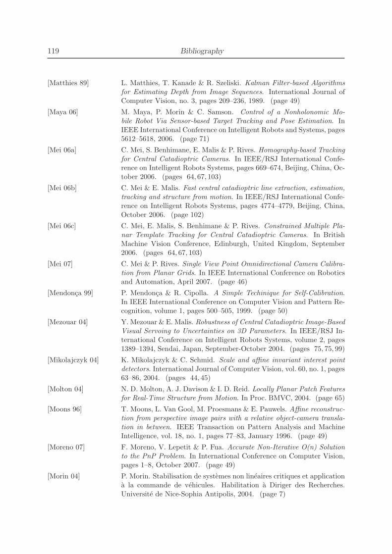
119 Bibliography
[Matthies 89] L. Matthies, T. Kanade & R. Szeliski. Kalman Filter-based Algorithmsfor Estimating Depth from Image Sequences. International Journal ofComputer Vision, no. 3, pages 209–236, 1989. (page 49)
[Maya 06] M. Maya, P. Morin & C. Samson. Control of a Nonholonomic Mo-bile Robot Via Sensor-based Target Tracking and Pose Estimation. InIEEE International Conference on Intelligent Robots and Systems, pages5612–5618, 2006. (page 71)
[Mei 06a] C. Mei, S. Benhimane, E. Malis & P. Rives. Homography-based Trackingfor Central Catadioptric Cameras. In IEEE/RSJ International Confe-rence on Intelligent Robots Systems, pages 669–674, Beijing, China, Oc-tober 2006. (pages 64, 67, 103)
[Mei 06b] C. Mei & E. Malis. Fast central catadioptric line extraction, estimation,tracking and structure from motion. In IEEE/RSJ International Confe-rence on Intelligent Robots Systems, pages 4774–4779, Beijing, China,October 2006. (page 102)
[Mei 06c] C. Mei, E. Malis, S. Benhimane & P. Rives. Constrained Multiple Pla-nar Template Tracking for Central Catadioptric Cameras. In BritishMachine Vision Conference, Edinburgh, United Kingdom, September2006. (pages 64, 67, 103)
[Mei 07] C. Mei & P. Rives. Single View Point Omnidirectional Camera Calibra-tion from Planar Grids. In IEEE International Conference on Roboticsand Automation, April 2007. (page 46)
[Mendonca 99] P. Mendonca & R. Cipolla. A Simple Techinique for Self-Calibration.In IEEE International Conference on Computer Vision and Pattern Re-cognition, volume 1, pages 500–505, 1999. (page 50)
[Mezouar 04] Y. Mezouar & E. Malis. Robustness of Central Catadioptric Image-BasedVisual Servoing to Uncertainties on 3D Parameters. In IEEE/RSJ In-ternational Conference on Intelligent Robots Systems, volume 2, pages1389–1394, Sendai, Japan, September-October 2004. (pages 75, 75, 99)
[Mikolajczyk 04] K. Mikolajczyk & C. Schmid. Scale and affine invariant interest pointdetectors. International Journal of Computer Vision, vol. 60, no. 1, pages63–86, 2004. (pages 44, 45)
[Molton 04] N. D. Molton, A. J. Davison & I. D. Reid. Locally Planar Patch Featuresfor Real-Time Structure from Motion. In Proc. BMVC, 2004. (page 65)
[Moons 96] T. Moons, L. Van Gool, M. Proesmans & E. Pauwels. Affine reconstruc-tion from perspective image pairs with a relative object-camera transla-tion in between. IEEE Transaction on Pattern Analysis and MachineIntelligence, vol. 18, no. 1, pages 77–83, January 1996. (page 49)
[Moreno 07] F. Moreno, V. Lepetit & P. Fua. Accurate Non-Iterative O(n) Solutionto the PnP Problem. In International Conference on Computer Vision,pages 1–8, October 2007. (page 49)
[Morin 04] P. Morin. Stabilisation de systemes non lineaires critiques et applicationa la commande de vehicules. Habilitation a Diriger des Recherches.Universite de Nice-Sophia Antipolis, 2004. (page 7)

Ezio Malis 120
[Nakamura 86] Y. Nakamura & H. Hanafusa. Inverse kinematics solutions with sin-gularity robustness for robot manipulator control. Transaction ASMEJournal of Dynamic Systems, Measurement and Control, vol. 108, pages163–171, September 1986. (page 73)
[Nister 04] D. Nister. An efficient solution to the five-point relative pose pro-blem. IEEE Transactions on Pattern Analysis and Machine Intelligence,vol. 26, no. 6, pages 756–770, 2004. (page 47)
[Nister 06] D. Nister, O. Naroditsky & J. Bergen. Visual Odometry for GroundVehicle Applications. Journal of Field Robotics, vol. 23, no. 1, 2006.(page 47)
[Pennec 99] X. Pennec, P. Cachier & N. Ayache. Understanding the “Demon’s Algo-rithm” : 3D Non-Rigid registration by Gradient Descent. In Int. Conf. onMedical Image Computing and Computer-Assisted Intervention (MIC-CAI’99), volume 1679 of LNCS, pages 597–605, Cambridge, UK, Sep-tember 1999. Springer Verlag. (page 54)
[Pollefeys 99] M. Pollefeys, R. Koch & L. VanGool. Self-Calibration and Metric Re-construction Inspite of Varying and Unknown Intrinsic Camera Para-meters. ijcv, vol. 32, no. 1, pages 7–25, August 1999. (page 50)
[Quarteroni 00] A. Quarteroni, R. Sacco & F. Salieri. Numerical mathematics. Springer-Verlag, 2000. (pages 17, 22)
[Rogel 06] P. Rogel & S. Kova. Symmetric image registration. Medical ImageAnalysis, vol. 10, no. 3, pages 484–493, 2006. (page 54)
[Royer 07] E. Royer, M. Lhuillier, M. Dhome & J. Lavest. Monocular vision for mo-bile robot localization and autonomous navigation. International Journalof Computer Vision, vol. 74, no. 3, pages 237–260, 2007. (page 47)
[Se 05] S. Se, D. Lowe & J. Little. Vision-based global localization and Mappingfor Mobile Robots. IEEE Transactions on Robotics and Automation,vol. 21, no. 3, pages 364–375, 2005. (page 47)
[Silveira 06a] G. Silveira, E. Malis & P. Rives. Real-time Robust Detection of PlanarRegions in a Pair of Images. In IEEE/RSJ International Conference onIntelligent Robots Systems, pages 49–54, Beijing, China, October 2006.(pages 68, 89, 104)
[Silveira 06b] G. Silveira, E. Malis & P. Rives. Visual Servoing over Unknown, Un-structured, Large-scale Scenes. In IEEE International Conference onRobotics and Automation, pages 4142–4147, Orlando, USA, May 2006.(pages 89, 90, 104)
[Silveira 07a] G. Silveira & E. Malis. Direct Visual Servoing with respect to RigidObjects. In IEEE Computer Vision and Pattern Recognition, San Diego,USA, October 2007. (pages 80, 81)
[Silveira 07b] G. Silveira & E. Malis. Real-time Visual Tracking under Arbitrary Illu-mination Changes. In IEEE Computer Vision and Pattern Recognition,Minneapolis, USA, June 2007. (pages 54, 59, 60, 103)

121 Bibliography
[Silveira 07c] G. Silveira, E. Malis & P. Rives. An Efficient Direct Method for Impro-ving visual SLAM. In IEEE International Conference on Robotics andAutomation, Rome, Italy, April 2007. (pages 65, 68, 89, 104)
[Smith 94] C. Smith & N. Papanikolopoulos. Computation of shape through control-led active exploration. In IEEE International Conference on Roboticsand Automation, volume 3, pages 2516–2521, San Diego, CA, USA,May 1994. (page 49)
[Stein 00] G. Stein & A. Shashua. Model-Based Brightness Constraints : On Di-rect Estimation of Structure and Motion. IEEE Transactions on PatternAnalysis and Machine Intelligence, vol. 22, no. 9, pages 992–1015, Sep-tember 2000. (page 43)
[Szeliski 95] R. Szeliski & S. Kang. Direct Method for Visual Scene Reconstruction.In IEEE Workshop on Representation of Visual Scenes, 1995. (page 54)
[Thirion 98] J. Thirion. Image matching as a diffusion process : an analogy withMaxwell’s demons. Medical Image Analysis, vol. 2, no. 3, pages 243–260, 1998. (page 54)
[Torr 98] P. Torr, A. W. Fitzgibbon & A. Zisserman. Maintaining Multiple MotionModel Hypotheses Over Many Views to Recover Matching and Structure.In IEEE International Conference on Computer Vision, pages 485–491,Bombay, India, January 1998. (page 47)
[Torr 00] P. H. S. Torr & A Zisserman. Feature Based Methods for Structure andMotion Estimation. In B. Triggs, A. Zisserman & R. Szeliski, editeurs,Vision Algorithms : Theory and practice, numero 1883 in Lecture Notesin Computer Science, pages 279–295. Springer-Verlag, September 2000.(page 43)
[Triggs 97] B. Triggs. Autocalibration and the Absolute Quadric. In IEEE Interna-tional Conference on Computer Vision and Pattern Recognition, pages609–614, 1997. (page 50)
[Triggs 98] B. Triggs. Autocalibration from planar scenes. In European Conferenceof Computer Vision, pages 89–105, 1998. (page 51)
[Triggs 00] B. Triggs, P. McLauchlan, R. Hartley & A. Fitzgibbon. Bundle Adjust-ment – A Modern Synthesis. In B. Triggs, A. Zisserman & R. Szeliski,editeurs, Vision Algorithms : Theory and Practice, volume 1883 of Lec-ture Notes in Computer Science, pages 298–372. Springer-Verlag, 2000.(pages 47, 50)
[Tsai 87] R.Y. Tsai. A versatile camera calibration technique for high-accuracy3D machine vision metrology using off-the-shelf TV cameras and lenses.IEEE Journal of Robotics and Automation, vol. 3, no. 4, pages 323–344,August 1987. (page 46)
[Tuytelaars 04] T. Tuytelaars & L. Van Gool. Matching widely separated views basedon affine invariant regions. International Journal of Computer Vision,vol. 59, no. 1, pages 61–85, 2004. (pages 44, 45)
[Varadarajan 74] V. Varadarajan. Lie groups, lie algebras, and their representation, vo-lume 102 of Graduate Texts in Mathematics. Prentice-Hall Inc., 1974.(pages 4, 5, 6, 32)

Ezio Malis 122
[Vargas 05] M. Vargas & E. Malis. Visual servoing based on an analytical homo-graphy decomposition. In IEEE Conf. on Decision and Control and Eu-ropean Control Conf., pages 5379–5384, Sevilla, Spain, December 2005.(pages 48, 80, 100)
[Vercauteren 07] T. Vercauteren, X. Pennec, E. Malis, A. Perchant & N. Ayache. InsightInto Efficient Image Registration Techniques and the Demons Algorithm.In Information Processing in Medical Imaging, Kerkrade, Netherlands,June 2007. (pages 54, 60, 102)
[Wampler 86] C. W. Wampler. Manipulator inverse kinematic solution based on vectorformulations and damped least squares methods. IEEE Transactions onSystem, Man, Cybernetics, vol. 16, no. 1, pages 93–101, 1986. (page 73)
[Wang 05] H. Wang, L. Dong, J. O’Daniel, R. Mohan, A. Garden, K Ang, D. Ku-ban, M. Bonnen, J. Chang & R. Cheung. Validation of an accelerated’demons’ algorithm for deformable image registration in radiation the-rapy. Physics in Medicine and Biology, vol. 50, no. 12, pages 2887–2905,June 2005. (page 54)
[Warner 71] Frank W. Warner. Foundations of differentiable manifolds and liegroups. Springer-Verlag, 1971. (pages 4, 5, 6, 32)
[Weiss 87] L. E. Weiss, A. C. Sanderson & C. P. Neuman. Dynamic Sensor-BasedControl of robots with Visual Feedback. IEEE Journal of Robotics andAutomation, vol. 3, no. 5, pages 404–417, October 1987. (page 72)
[Weng 92] J. Weng, P. Cohen & M. Herniou. Camera calibration with distortionmodels and accuracy evaluation. IEEE Transactions on Pattern Analysisand Machine Intelligence, vol. 14, no. 10, pages 965–980, October 1992.(pages 9, 46)
[Wilson 96] W. J. Wilson, C. C. W. Hulls & G. S. Bell. Relative End-Effector ControlUsing Cartesian Position-Based Visual Servoing. IEEE Transactions onRobotics and Automation, vol. 12, no. 5, pages 684–696, October 1996.(page 89)
[Zhang 96] Z. Zhang & A. R. Hanson. 3D Reconstruction Based on HomographyMapping. In ARPA Image Understanding Workshop, Palm Springs, CA,1996. (page 48)
[Zhang 00] Z. Zhang. A flexible new technique for camera calibration. IEEE Tran-saction on Pattern Analysis and Machine Intelligence, vol. 22, no. 11,pages 1330–1334, 2000. (page 46)
[Zitova 03] B. Zitova & J. Flusser. Image registration methods : a survey. Imageand Vision Computing, vol. 21, no. 11, pages 977–1000, October 2003.(page 53)