Visibility Metric for Visually LosslessImage Compression

Nanyang Ye1, Marıa Perez-Ortiz1,2, and Rafał K. Mantiuk1

1Department of Computer Science and Technology, University of Cambridge, Cambridge, United KingdomEmail: {yn272, rafal.mantiuk}@cl.cam.ac.uk

2Department of Computer Science, University College London, London, United KingdomEmail: maria.perez@ucl.ac.uk

Abstract—Encoding images in a visually lossless manner helpsto achieve the best trade-off between image compression perfor-mance and quality and so that compression artifacts are invisibleto the majority of users. Visually lossless encoding can oftenbe achieved by manually adjusting compression quality param-eters of existing lossy compression methods, such as JPEG orWebP. But the required compression quality parameter can alsobe determined automatically using visibility metrics. However,creating an accurate visibility metric is challenging because of thecomplexity of the human visual system and the effort needed tocollect the required data. In this paper, we investigate how to trainan accurate visibility metric for visually lossless compression froma relatively small dataset. Our experiments show that predictionerror can be reduced by 40% compared with the state-of-the-art, and that our proposed method can save between 25%-75%of storage space compared with the default quality parameterused in commercial software. We demonstrate how the visibilitymetric can be used for visually lossless image compression andfor benchmarking image compression encoders.

Index Terms—Visually lossless image compression, visibilitymetric, deep learning, transfer learning

I. INTRODUCTION

The enormous amount of image and video data on theInternet poses a significant challenge for data transmission andstorage. While significant effort has been invested in betterimage and video coding methods, improving these methodsaccording to the human visual system’s perception of visualquality.

Image and video compression methods can be categorizedas lossy or lossless. While lossless methods retain origi-nal information up to the bit-precision of the digital rep-resentation, they are several times less efficient than lossymethods. Visually lossless methods lie in between lossy andlossless compression: they introduce compression distortions,but ensure that those distortions are unlikely to be visible.Visually lossless compression was first introduced to compressmedical images and handle the increasing amount of data inclinics’ picture archiving [1]. By selecting a fixed compressionparameter or modifying the compression encoders, visuallylossless compression has been shown effective for medicalimages in the gray-scale domain [2]. However, previous re-search on visually lossless compression is largely content andencoder dependent, which means we cannot apply medical

compression methods to the compression of general imagecontent using popular compression methods, such as JPEG.The goal of this paper is to devise a content and encoderindependent visually lossless compression method for naturalimages.

While image quality metrics (IQMs) are meant to predictthe perceived magnitude of impairment [3], visibility metricspredict the probability of noticing the impairment. IQMs arethus well suited for predicting strong, suprathreshold distor-tions. However, visibility metrics tend to be more accuratewhen predicting barely noticeable artifacts. Eckert et al. foundthat objective quality scores produced by IQMs (e.g. meansquared error), are correlated with compression quality setting[4]. However, simple IQMs have been found inaccurate [5].

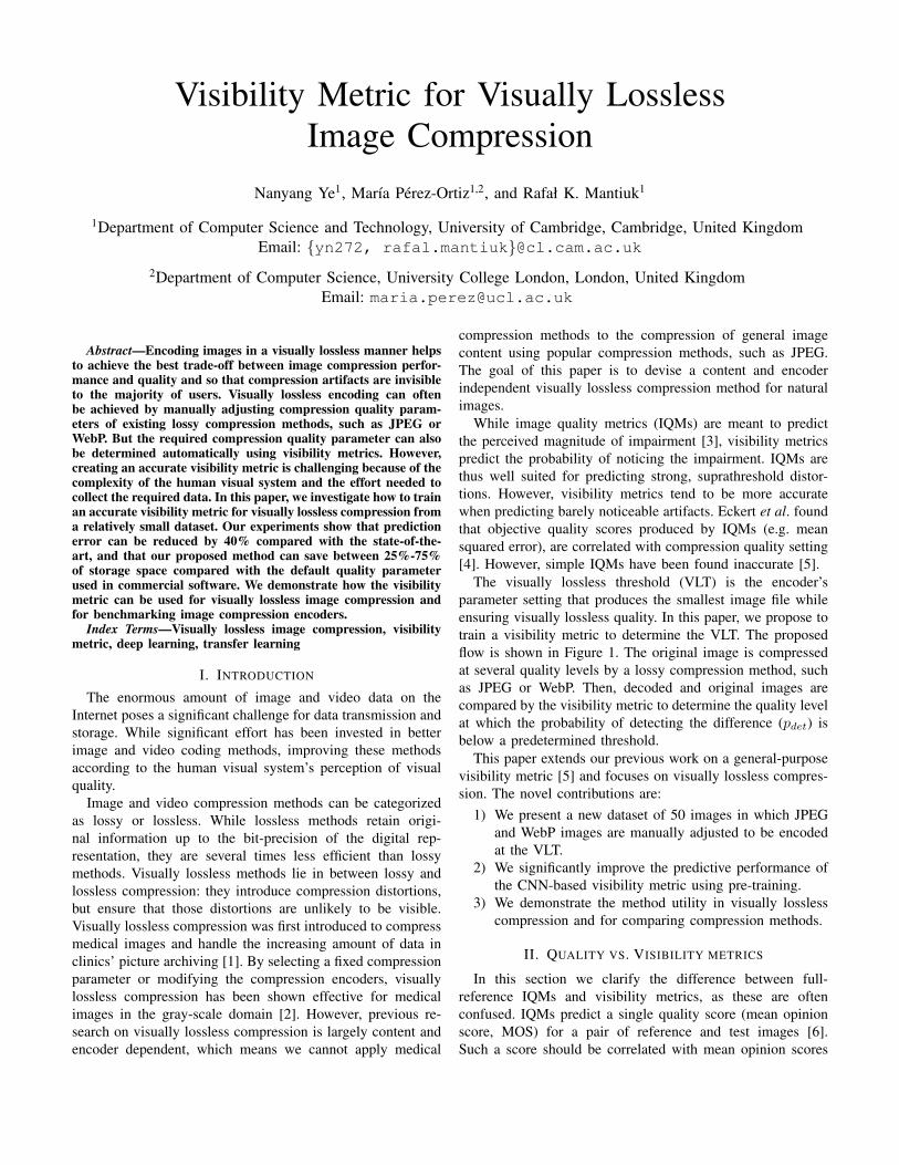
The visually lossless threshold (VLT) is the encoder’sparameter setting that produces the smallest image file whileensuring visually lossless quality. In this paper, we propose totrain a visibility metric to determine the VLT. The proposedflow is shown in Figure 1. The original image is compressedat several quality levels by a lossy compression method, suchas JPEG or WebP. Then, decoded and original images arecompared by the visibility metric to determine the quality levelat which the probability of detecting the difference (pdet) isbelow a predetermined threshold.

This paper extends our previous work on a general-purposevisibility metric [5] and focuses on visually lossless compres-sion. The novel contributions are:

1) We present a new dataset of 50 images in which JPEGand WebP images are manually adjusted to be encodedat the VLT.

2) We significantly improve the predictive performance ofthe CNN-based visibility metric using pre-training.

3) We demonstrate the method utility in visually losslesscompression and for comparing compression methods.

II. QUALITY VS. VISIBILITY METRICS

In this section we clarify the difference between full-reference IQMs and visibility metrics, as these are oftenconfused. IQMs predict a single quality score (mean opinionscore, MOS) for a pair of reference and test images [6].Such a score should be correlated with mean opinion scores

Visually lossless

compression

setting

Visibility

metric

Compression

encoder

Original image Compressed image

Visibility prediction

Fig. 1. Proposed flow of our method for visually lossless compression basedon visibility metrics.

collected in subjective image quality assessment experiments.An extensive review of IQMs, including SSIM, VSI, FSIM,can be found in the survey [3].

However, it is challenging to estimate VLT accurately fromtraditional subjective assessment experiments, since meanopinion scores only capture overall image quality and do notexplain where the distortions are visible in an image. This willbe demonstrated with experiments in Section IV.

Visibility metrics predict the probability that the averageobserver [7] or a percentage of the population [5] will noticethe difference between a pair of images. This probability ispredicted locally, for pixels or image patches. The maximumvalue from such a probability map is computed to obtaina conservative estimate of the overall detection probability.Visibility metrics are either based on models of low-levelhuman vision [7], [8] or rely on machine learning, trainedusing locally labeled images [5]. This paper improves on theCNN-based metric from [5] with the help of a newly collecteddataset and a new pre-training approach.

III. VISUALLY LOSSLESS IMAGE COMPRESSION DATASET

With the aim of validating visibility metrics, we collect a vi-sually lossless image compression (VLIC) dataset, containingimages encoded with JPEG and WebP1 codecs.

A. Stimuli

The VLIC dataset consists of 50 reference scenes comingfrom previous image compression and image quality studies.The stimuli are taken from the Rawzor’s free dataset (14images)2, CSIQ dataset (30 images) [9] and the subjectivequality dataset in [10] (where we randomly selected 6 imagesfrom the 10 images in the dataset). For Rawzor’s dataset,images were cropped to 960x600 pixels to fit on our screen.These images provide a variety of contents, including por-traits, landscapes, daylight and night scenes. The images wereselected to be a representative sample of Internet content.For JPEG compression, we use the standard JPEG codec(libjpeg3). For WebP compression, we use the WebP codec

1https://developers.google.com/speed/webp/2http://imagecompression.info/test images/3https://github.com/LuaDist/libjpeg

(libwebp4). Half of the reference scenes is compressed withJPEG and the other half with WebP, each into 50 differentcompression levels.

B. Experiment Procedure

The experimental task was to find the compression levelat which observers cannot distinguish between the referenceimage and the compressed image.

1) Experiment stages: The experiment consisted of twostages. In the first stage, observers were presented with ref-erence and compressed images side-by-side, and asked toadjust the compression level of the compressed image untilthey could not see the difference (method-of-adjustment).Compression levels found in the first stage were used as theinitial guess for a more accurate 4-alternative-force-choice pro-cedure (4AFC), used in the second stage. In this second stage,observers were shown 3 reference and 1 distorted images inrandom order and asked to select the distorted one. QUESTmethod [11] was used for adaptive sampling of compressionlevels and for fitting a psychometric function. Between 20and 30 4AFC trials were collected per participant for eachimage. We decided to use side-by-side presentation rather thanflicker technique from IEC 29170-2 standard [12] because thelatter leads to overly conservative VLT as visual system is verysensitive to flicker. The side-by-side presentation is also closerto the scenario that users are likely to use in practice whenassessing compression quality. On average, it took between 2and 5 minutes for each observer to complete measurementsfor a single image.

2) Viewing Condition: The experiments were conducted ina dark room. Observers sat 90 cm from a 24 inch, 1920x1200resolution NEC MultiSync PA241W display, which corre-sponds to the angular resolution of 60 pixels per visual degree.The viewing distance was controlled with a chinrest.

3) Observers: Observers were students and university staffwith normal or corrected to normal vision. We collected datafrom 19 observers aged between 20 and 30 years. Around 10measurements were collected for each image.

IV. QUALITY METRICS FOR VISUALLY LOSSLESS IMAGECOMPRESSION

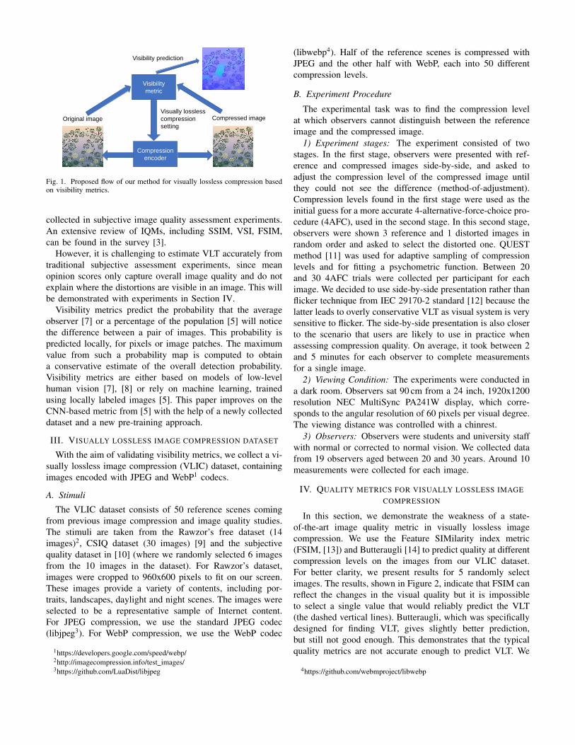
In this section, we demonstrate the weakness of a state-of-the-art image quality metric in visually lossless imagecompression. We use the Feature SIMilarity index metric(FSIM, [13]) and Butteraugli [14] to predict quality at differentcompression levels on the images from our VLIC dataset.For better clarity, we present results for 5 randomly selectimages. The results, shown in Figure 2, indicate that FSIM canreflect the changes in the visual quality but it is impossibleto select a single value that would reliably predict the VLT(the dashed vertical lines). Butteraugli, which was specificallydesigned for finding VLT, gives slightly better prediction,but still not good enough. This demonstrates that the typicalquality metrics are not accurate enough to predict VLT. We

4https://github.com/webmproject/libwebp

made a similar observation when testing other quality metrics,both full-reference and non-reference.

0 20 40 60 80 100Compression quality

3.5

3.0

2.5

2.0

1.5

1.0

0.5

log 1

0(1-

FSIM

)

elkturtlebostonbridgeartificial

0 20 40 60 80 100Compression quality

0.0

0.5

1.0

1.5

log 1

0(Bu

ttera

ugli)

elkturtlebostonbridgeartificial

Fig. 2. The predictions of FSIM (top) and Butteraugli (bottom) for imagescompressed with increasing compression quality. The vertical dashed linesdenote the visually lossless threshold (VLT) from the experiment with thesame color denoting the same image. The predictions of existing metrics arenot good indicators of VLT.

V. DEEP NEURAL NETWORK FOR VISUALLY LOSSLESSCOMPRESSION

In this section, we summarize the architecture from ourprevious work [5] and explore pre-training strategies to achievean accurate metric even when only using a small dataset.

A. Architecture of the visibility metric

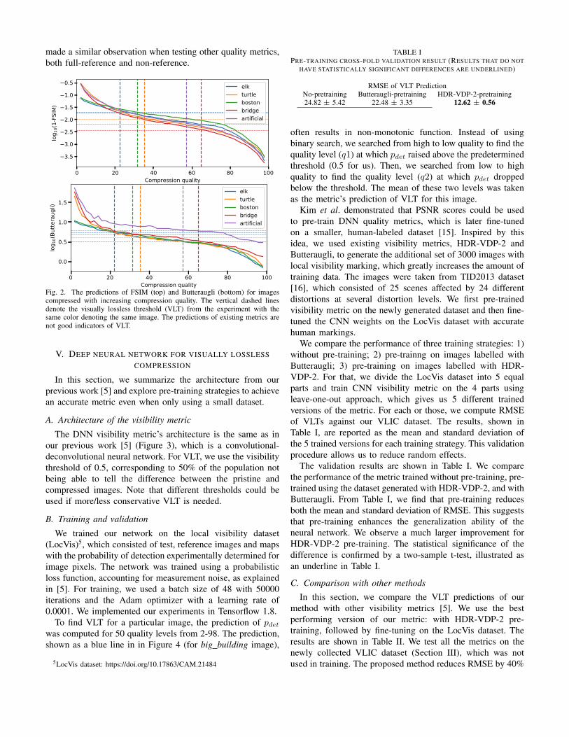
The DNN visibility metric’s architecture is the same as inour previous work [5] (Figure 3), which is a convolutional-deconvolutional neural network. For VLT, we use the visibilitythreshold of 0.5, corresponding to 50% of the population notbeing able to tell the difference between the pristine andcompressed images. Note that different thresholds could beused if more/less conservative VLT is needed.

B. Training and validation

We trained our network on the local visibility dataset(LocVis)5, which consisted of test, reference images and mapswith the probability of detection experimentally determined forimage pixels. The network was trained using a probabilisticloss function, accounting for measurement noise, as explainedin [5]. For training, we used a batch size of 48 with 50000iterations and the Adam optimizer with a learning rate of0.0001. We implemented our experiments in Tensorflow 1.8.

To find VLT for a particular image, the prediction of pdetwas computed for 50 quality levels from 2-98. The prediction,shown as a blue line in in Figure 4 (for big building image),

5LocVis dataset: https://doi.org/10.17863/CAM.21484

TABLE IPRE-TRAINING CROSS-FOLD VALIDATION RESULT (RESULTS THAT DO NOT

HAVE STATISTICALLY SIGNIFICANT DIFFERENCES ARE UNDERLINED)

RMSE of VLT PredictionNo-pretraining Butteraugli-pretraining HDR-VDP-2-pretraining24.82 ± 5.42 22.48 ± 3.35 12.62 ± 0.56

often results in non-monotonic function. Instead of usingbinary search, we searched from high to low quality to find thequality level (q1) at which pdet raised above the predeterminedthreshold (0.5 for us). Then, we searched from low to highquality to find the quality level (q2) at which pdet droppedbelow the threshold. The mean of these two levels was takenas the metric’s prediction of VLT for this image.

Kim et al. demonstrated that PSNR scores could be usedto pre-train DNN quality metrics, which is later fine-tunedon a smaller, human-labeled dataset [15]. Inspired by thisidea, we used existing visibility metrics, HDR-VDP-2 andButteraugli, to generate the additional set of 3000 images withlocal visibility marking, which greatly increases the amount oftraining data. The images were taken from TID2013 dataset[16], which consisted of 25 scenes affected by 24 differentdistortions at several distortion levels. We first pre-trainedvisibility metric on the newly generated dataset and then fine-tuned the CNN weights on the LocVis dataset with accuratehuman markings.

We compare the performance of three training strategies: 1)without pre-training; 2) pre-trainng on images labelled withButteraugli; 3) pre-training on images labelled with HDR-VDP-2. For that, we divide the LocVis dataset into 5 equalparts and train CNN visibility metric on the 4 parts usingleave-one-out approach, which gives us 5 different trainedversions of the metric. For each or those, we compute RMSEof VLTs against our VLIC dataset. The results, shown inTable I, are reported as the mean and standard deviation ofthe 5 trained versions for each training strategy. This validationprocedure allows us to reduce random effects.

The validation results are shown in Table I. We comparethe performance of the metric trained without pre-training, pre-trained using the dataset generated with HDR-VDP-2, and withButteraugli. From Table I, we find that pre-training reducesboth the mean and standard deviation of RMSE. This suggeststhat pre-training enhances the generalization ability of theneural network. We observe a much larger improvement forHDR-VDP-2 pre-training. The statistical significance of thedifference is confirmed by a two-sample t-test, illustrated asan underline in Table I.

C. Comparison with other methods

In this section, we compare the VLT predictions of ourmethod with other visibility metrics [5]. We use the bestperforming version of our metric: with HDR-VDP-2 pre-training, followed by fine-tuning on the LocVis dataset. Theresults are shown in Table II. We test all the metrics on thenewly collected VLIC dataset (Section III), which was notused in training. The proposed method reduces RMSE by 40%

Reference Patch 48x48

Conv1 96@12x12 batchnorm1 pool1@5x5

Conv2 256@5x5batchnorm2

pool2@2x2

Conv1 96@12x12 batchnorm1 pool1@5x5

Conv2 256@5x5batchnorm2

pool2@2x2

Concate512@2x2 Upsampling

@5x5 Upsampling2@12x12

Conv3512@3x3

Conv4256@3x3 Conv5

96@3X3Conv696@3x3

Upsampling3@48X48

Conv796@3x3

Test Patch 48x48

Fig. 3. The CNN architecture. We use the non-Siamese fully-convolutional neural network to predict visibility maps.

0 20 40 60 80 100Quality

0.2

0.4

0.6

0.8

1.0

Pdet

q1q2q

Fig. 4. Illustration of the procedure used to determine the visually losslessthreshold using the visibility metric.

TABLE IIEXPERIMENT RESULTS ON THE VISUALLY LOSSLESS IMAGE

COMPRESSION DATASET

RMSE of VLT PredictionProposed CNN [5] Butteraugli [14] HDR-VDP-2 [7]

12.38 20.33 20.91 43.33

compared with the best-performing CNN-based metric fromour previous work.

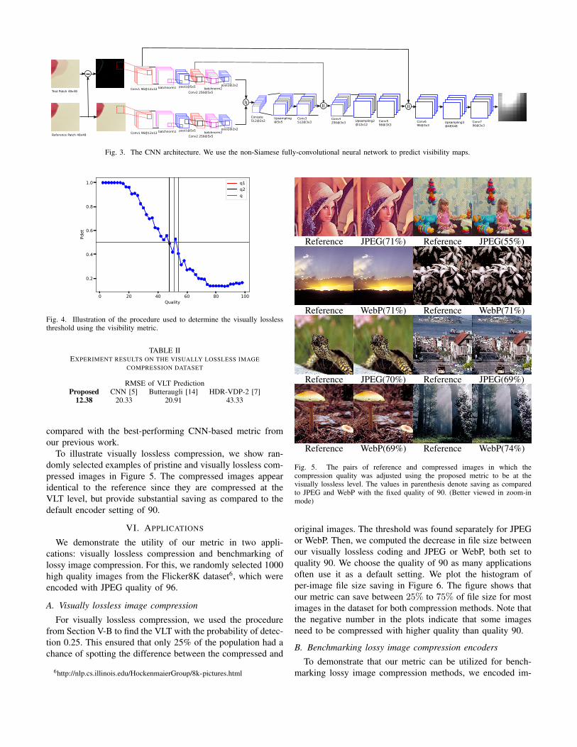
To illustrate visually lossless compression, we show ran-domly selected examples of pristine and visually lossless com-pressed images in Figure 5. The compressed images appearidentical to the reference since they are compressed at theVLT level, but provide substantial saving as compared to thedefault encoder setting of 90.

VI. APPLICATIONS

We demonstrate the utility of our metric in two appli-cations: visually lossless compression and benchmarking oflossy image compression. For this, we randomly selected 1000high quality images from the Flicker8K dataset6, which wereencoded with JPEG quality of 96.

A. Visually lossless image compression

For visually lossless compression, we used the procedurefrom Section V-B to find the VLT with the probability of detec-tion 0.25. This ensured that only 25% of the population had achance of spotting the difference between the compressed and

6http://nlp.cs.illinois.edu/HockenmaierGroup/8k-pictures.html

Reference JPEG(71%) Reference JPEG(55%)

Reference WebP(71%) Reference WebP(71%)

Reference JPEG(70%) Reference JPEG(69%)

Reference WebP(69%) Reference WebP(74%)

Fig. 5. The pairs of reference and compressed images in which thecompression quality was adjusted using the proposed metric to be at thevisually lossless level. The values in parenthesis denote saving as comparedto JPEG and WebP with the fixed quality of 90. (Better viewed in zoom-inmode)

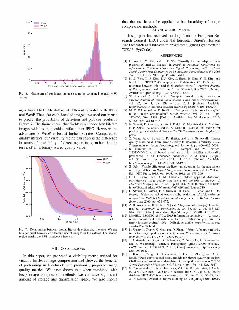
original images. The threshold was found separately for JPEGor WebP. Then, we computed the decrease in file size betweenour visually lossless coding and JPEG or WebP, both set toquality 90. We choose the quality of 90 as many applicationsoften use it as a default setting. We plot the histogram ofper-image file size saving in Figure 6. The figure shows thatour metric can save between 25% to 75% of file size for mostimages in the dataset for both compression methods. Note thatthe negative number in the plots indicate that some imagesneed to be compressed with higher quality than quality 90.

B. Benchmarking lossy image compression encoders

To demonstrate that our metric can be utilized for bench-marking lossy image compression methods, we encoded im-

100 75 50 25 0 25 50 75 100Per-image storage space saving in percent

0

20

40

60

80

100Fr

eque

ncy

JPEGWebP

Fig. 6. Histogram of per-image storage saving as compared to quality 90setting.

ages from Flicker8K dataset at different bit-rates with JPEGand WebP. Then, for each decoded images, we used our metricto predict the probability of detection and plot the results inFigure 7. The figure shows that WebP can encode low bit-rateimages with less noticeable artifacts than JPEG. However, theadvantage of WebP is lost at higher bit-rates. Compared toquality metrics, our visibility metric can express the differencein terms of probability of detecting artifacts, rather than interms of an arbitrary scaled quality value.

0.5 1.0 1.5 2.0 2.5Bit per pixel

0.0

0.2

0.4

0.6

0.8

1.0

Prob

abilit

y of

det

ectio

n (P

det)

JPEGWEBP

Fig. 7. Relationship between probability of detection and file size. We usebits-per-pixel because of different size of images in the dataset. The shadedregion marks the 95% confidence interval.

VII. CONCLUSIONS

In this paper, we proposed a visibility metric trained forvisually lossless image compression and showed the benefitsof pretraining such network with previously proposed imagequality metrics. We have shown that when combined withlossy image compression methods, we can save significantamount of storage and transmission space. We also shown

that the metric can be applied to benchmarking of imagecompression methods.

ACKNOWLEDGEMENTS

This project has received funding from the European Re-search Council (ERC) under the European Union’s Horizon2020 research and innovation programme (grant agreement n◦

725253–EyeCode).REFERENCES

[1] D. Wu, D. M. Tan, and H. R. Wu, “Visually lossless adaptive com-pression of medical images,” in Fourth International Conference onInformation, Communications and Signal Processing, 2003 and theFourth Pacific Rim Conference on Multimedia. Proceedings of the 2003Joint, vol. 1, Dec 2003, pp. 458–463 Vol.1.

[2] H. S. Woo, K. J. Kim, T. J. Kim, S. Hahn, B. Kim, Y. H. Kim, andK. H. Lee, “JPEG 2000 compression of abdominal CT: Difference intolerance between thin- and thick-section images,” American Journalof Roentgenology, vol. 189, no. 3, pp. 535–541, Sep 2007. [Online].Available: https://doi.org/10.2214/AJR.07.2304

[3] W. Lin and C.-C. J. Kuo, “Perceptual visual quality metrics: Asurvey,” Journal of Visual Communication and Image Representation,vol. 22, no. 4, pp. 297 – 312, 2011. [Online]. Available:http://www.sciencedirect.com/science/article/pii/S1047320311000204

[4] M. P. Eckert and A. P. Bradley, “Perceptual quality metrics appliedto still image compression,” Signal Process., vol. 70, no. 3, pp.177–200, Nov. 1998. [Online]. Available: http://dx.doi.org/10.1016/S0165-1684(98)00124-8

[5] K. Wolski, D. Giunchi, N. Ye, P. Didyk, K. Myszkowski, R. Mantiuk,H.-P. Seidel, A. Steed, and R. K. Mantiuk, “Dataset and metrics forpredicting local visible differences,” ACM Transactions on Graphics, inpress.

[6] Z. Wang, A. C. Bovik, H. R. Sheikh, and E. P. Simoncelli, “Imagequality assessment: From error visibility to structural similarity,” IEEETransactions on Image Processing, vol. 13, no. 4, pp. 600–612, 2004.

[7] R. Mantiuk, K. J. Kim, A. G. Rempel, and W. Heidrich,“HDR-VDP-2: A calibrated visual metric for visibility and qualitypredictions in all luminance conditions,” ACM Trans. Graph.,vol. 30, no. 4, pp. 40:1–40:14, Jul. 2011. [Online]. Available:http://doi.acm.org/10.1145/2010324.1964935

[8] S. Daly, “Visible differences predictor: an algorithm for the assessmentof image fidelity,” in Digital Images and Human Vision, A. B. Watson,Ed. MIT Press, 1993, vol. 1666, no. 1992, pp. 179–206.

[9] E. C. Larson and D. M. Chandler, “Most apparent distortion:full-reference image quality assessment and the role of strategy.” J.Electronic Imaging, vol. 19, no. 1, p. 011006, 2010. [Online]. Available:http://dblp.uni-trier.de/db/journals/jei/jei19.html#LarsonC10

[10] C. Strauss, F. Pasteau, F. Autrusseau, M. Babel, L. Bedat, and O. De-forges, “Subjective and objective quality evaluation of LAR coded artimages,” in 2009 IEEE International Conference on Multimedia andExpo, June 2009, pp. 674–677.

[11] A. B. Watson and D. G. Pelli, “Quest: A bayesian adaptive psychometricmethod,” Perception & Psychophysics, vol. 33, no. 2, pp. 113–120,Mar 1983. [Online]. Available: https://doi.org/10.3758/BF03202828

[12] ISO/IEC, “ISO/IEC 29170-2:2015 Information technology – Advancedimage coding and evaluation – Part 2: Evaluation procedure fornearly lossless coding,” 1995. [Online]. Available: https://www.iso.org/standard/66094.html

[13] L. Zhang, L. Zhang, X. Mou, and D. Zhang, “Fsim: A feature similarityindex for image quality assessment,” Image Processing, IEEE Transac-tions on, vol. 20, pp. 2378 – 2386, 09 2011.

[14] J. Alakuijala, R. Obryk, O. Stoliarchuk, Z. Szabadka, L. Vandevenne,and J. Wassenberg, “Guetzli: Perceptually guided JPEG encoder,”CoRR, vol. abs/1703.04421, 2017. [Online]. Available: http://arxiv.org/abs/1703.04421

[15] J. Kim, H. Zeng, D. Ghadiyaram, S. Lee, L. Zhang, and A. C.Bovik, “Deep convolutional neural models for picture-quality prediction:Challenges and solutions to data-driven image quality assessment,” IEEESignal Processing Magazine, vol. 34, no. 6, pp. 130–141, Nov 2017.

[16] N. Ponomarenko, L. Jin, O. Ieremeiev, V. Lukin, K. Egiazarian, J. Astola,B. Vozel, K. Chehdi, M. Carli, F. Battisti, and C.-C. Jay Kuo, “Imagedatabase TID2013,” Image Commun., vol. 30, no. C, pp. 57–77, Jan.2015. [Online]. Available: http://dx.doi.org/10.1016/j.image.2014.10.009