Viscous symmetric stability of circular ﬂows - SOEST · and their fully nonlinear evolution (see...

J. Fluid Mech. (2010), vol. 652, pp. 171–193. c© Cambridge University Press 2010

doi:10.1017/S0022112009994149

171

Viscous symmetric stability of circular flows

R. C. KLOOSTERZIEL†School of Ocean and Earth Science and Technology, University of Hawaii, Honolulu, HI 96822, USA

(Received 20 July 2009; revised 18 December 2009; accepted 20 December 2009)

The linear stability properties of viscous circular flows in a rotating environmentare studied with respect to symmetric perturbations. Through the use of an effectiveenergy or Lyapunov functional, we derive sufficient conditions for Lyapunov stabilitywith respect to such perturbations. For circular flows with swirl velocity V (r) wefind that Lyapunov stability is determined by the properties of the function F(r) =(2V/r + f )/Q (with f the Coriolis parameter, r the radius and Q the absolutevorticity) instead of the customary Rayleigh discriminant Φ(r) = (2V/r + f )Q. Theconditions for stability are valid for flows with non-zero Q everywhere. Further, theflows are presumed stationary, incompressible and velocity perturbations are requiredto vanish at rigid boundaries. For Lyapunov stable flows an upper bound for theincrease of the total perturbation energy due to transient non-modal growth is derivedwhich is valid for any Reynolds number. The theory is applied to Couette flow andthe Lamb–Oseen vortex.

1. IntroductionIn Kloosterziel & Carnevale (2007) we studied the linear stability of some simple

baroclinic parallel shear flows in rotating stratified systems through the use ofappropriate Lyapunov functionals. The flows were assumed zonally invariant andsubjected to perturbations that are also zonally invariant. The instability that mayor may not ensue is sometimes called inertial instability. It is closely related tocentrifugal instability, which is a well-known robust phenomenon observed in circularflows subjected to perturbations that are also circularly symmetric. In the laboratorycentrifugal instability manifests itself, for example, as the famous axisymmetricTaylor vortices in Couette flow, i.e. the flow between two co-axial rotating cylinders.Because of the zonal invariance of disturbances in parallel shear flows and thecircularly symmetric nature of the disturbances of circular flows, both instabilities areappropriately called symmetric instability. In the older meteorological literature it issometimes called dynamic instability. For graphs from numerical simulations showingthe toroidal overturning motions associated with the centrifugal instability in vorticesand their fully nonlinear evolution (see e.g. Kloosterziel, Carnevale & Orlandi 2007).A sketch of the overturning motions associated with the toroidal vortices is providedin figure 1(a). Unlike in Kloosterziel & Carnevale (2007), in this paper we considerthe more complicated question of stability of ‘arbitrary’ circular flows but we restrictourselves to flows in a homogeneous fluid.

† Email address for correspondence: [email protected]

172 R. C. Kloosterziel

regionUnstable

f(a) (b)

θez

er eθ

V

w

vu

r

z

Figure 1. (a) Symmetric instability starts in an unstable region as toroidal vortices (‘ribvortices’) of alternating sign. For a barotropic vortex with swirl velocity V (r) the unstableregion is where the Rayleigh discriminant Φ(r) < 0 with Φ(r) defined in (1.1). (b) Diagramdefining the polar coordinate system and velocity components for a circular vortex. Here v isthe swirl velocity, w the vertical velocity component and u the radial velocity component.

For arbitrary barotropic circular flows with swirl velocity V (r), the inviscid classicalcondition for stability is that for all r:

Φ(r) > 0, where Φ =

(2V

r+ f

)Q and Q =

dV

dr+

V

r+ f = ω + f

(1.1)

is the absolute vorticity. The inviscid classical condition for instability is that Φ(r) <

0 in some region. The cylindrical polar coordinate system (r, θ, z) is sketched infigure 1(b). The relative vorticity component ω is in the z direction and aligned withthe axis of rotation and gravitational acceleration. At the time unfamiliar with theolder meteorological literature, Kloosterziel & van Heijst (1991) ‘rediscovered’ thecriterion in an attempt to explain the difficulty in creating stable anticyclones in arotating fluid in the laboratory. When f = 0 the condition Φ(r) < 0 reduces toRayleigh’s celebrated circulation criterion (Rayleigh 1916) for symmetric instability(see Drazin & Reid 1981). In an extension of Bayly’s analysis (Bayly 1988) to rotatingsystems, Sipp & Jacquin (2000) generalized the criterion to non-circular flows. InΦ the term 2V/r is replaced by 2|V |/R, with |V | the velocity amplitude along astreamline and R the local algebraic radius of curvature of the streamline. If thereare streamlines along which Φ < 0, then locally instability is guaranteed.

The classical criterion (1.1) for barotropic circular flows in a homogeneous fluidfollows from the classical condition for baroclinic circular flows with swirl velocityV (r, z) in a stably stratified fluid. If the fluid is Boussinesq, the criterion for stabilityis that everywhere in the domain:

N2 + Φ > 0 and N2Φ − S2 > 0, where S =

(2V

r+ f

)∂V

∂z, (1.2)

and N2 the square of the buoyancy frequency. Both criteria (1.1) and the generalcriterion (1.2) have long been known to meteorologists (see e.g. Sawyer 1947; vanMieghem 1951; Eliassen & Kleinschmidt 1957; Charney 1973). The second conditionin (1.2) appears in various disguises in the literature. The criterion for symmetricstability of barotropic and baroclinic parallel shear flows in a rotating system followquickly by discarding the curvature term 2V/r in Φ and for baroclinic flows in S aswell.

Viscous symmetric stability of circular flows 173

The classical stability criterion (1.2) for baroclinic flows pertains only to inviscid andadiabatic fluids and can be established in a variety of well-known ways. For instance,it can be established by including rotation and stratification in Rayleigh’s fluid ringexchange argument for circular vortices (Rayleigh 1916). The ‘pressureless’ Lagrangiandisplacement argument of Solberg (1936) also leads to the stability condition. Fjørtoft(1950) used an energy method which, unlike in Rayleigh’s or Solberg’s approach,takes continuity, boundary conditions and pressure perturbations into account. Usingthe fact that for symmetric perturbations the angular momentum or circulationof individual fluid rings is conserved, Fjørtoft showed that the combination oftotal kinetic energy associated with the azimuthal (swirl) velocity and the potentialenergy forms an effective potential energy for motions in the meridional rz plane.This effective potential energy depends only on the meridional displacement field.Fjørtoft further showed that the effective potential energy for a given basic flowis a minimum if the criterion for stability (1.2) is satisfied. If so, it follows thatthe increase in the total meridional kinetic energy can be kept arbitrarily small ifthe initial velocity perturbations and initial meridional displacements are sufficientlysmall.

Through a consideration of the time evolution of certain volume integratedquantities, Ooyama (1966) also found that in the linearized dynamics the totalmeridional kinetic energy and the meridional displacement field can be kept arbitrarilysmall if the classical condition for stability (1.2) is satisfied. If not, then initialperturbations can be introduced which lead to unbounded growth of both integralquantities, i.e. there will be instability. For the instability proof, Ooyama used aclever construction having noted that the assumption of the existence of normal-modes solutions may be erroneous, i.e. generally the linearized dynamics allows fora normal-modes analysis only when the boundaries have a special shape, whichdiffers for different flows (see Høiland 1962; Yanai & Tokiaka 1969). Thus, normal-modes stability/instability or so-called exponential stability/instability can rarelybe expected to be established for enclosed flows. If the question of the existenceof normal-modes solutions is disregarded, a normal-modes analysis does howeverlead to the inviscid criterion for stability. For barotropic flows in a homogeneousfluid this is shown in the Appendix, i.e. if (1.1) holds, there will be normal-modesstability.

For baroclinic parallel shear flows in a rotating system, Cho, Shepherd & Vladimirov(1993) as well as Mu, Shepherd & Swanson (1996) showed that nonlinear stabilityin the sense of Lyapunov follows if (1.2) is satisfied. They used the energy-Casimirmethodology of Fjørtoft (1950) and Arnol’d (1966). It requires the introduction ofa ‘pseudo-energy’. The difference between the pseudo-energy of the perturbed flowand the basic unperturbed state is the disturbance pseudo-energy which is conservedin the fully nonlinear dynamics. If (1.2) is satisfied, the disturbance pseudo-energyis a positive-definite functional of the finite-amplitude perturbations which impliesLyapunov stability.

In Kloosterziel & Carnevale (2007) it was shown how the presumed symmetry inthe linear perturbation problem allows for the construction of an ‘effective energy’ Ewhich also establishes stability in the sense of Lyapunov if the classical condition (1.2)is satisfied. The disturbance pseudo-energy of Cho et al. (1993) reduces in the small-amplitude limit to this effective energy. The stability proofs of Fjørtoft (1950), Ooyama(1966) and Cho et al. (1993) all depend on conservation of angular momentum orabsolute velocity as well as density of individual fluid rings or rods. If viscosityand density diffusion are included, these conservation laws no longer hold. But, the


construction of Kloosterziel & Carnevale (2007) allows for the inclusion of viscosityand density diffusion (albeit just for the linearized dynamics). With their approach theyrediscovered McIntyre’s stability boundary for ‘double diffusive’ instability (McIntyre1970). McIntyre found this stability boundary with a normal-modes analysis onan unbounded domain (approximating a circular flow by a rectilinear flow withconstant vertical and horizontal shear and embedded in a fluid with constantbuoyancy frequency) in the limit of vanishing viscosity. This favourable comparisonled us to expect that by using Kloosterziel and Carnevale’s approach (Kloosterziel& Carnevale 2007) we might be able to extract useful information regardingstability of more realistic viscous/diffusive flows. The first step in this directionis taken in this paper by considering arbitrary circular flows in a homogeneousfluid.

The plan of this paper is as follows. Section 2 starts with the linear perturbationequations. In § 2.1 we construct the effective energy E which is conserved in theinviscid linear dynamics, i.e. dE/dt = 0, where t is time. The construction is onlyvalid for flows for which the (absolute) vorticity Q is sign-definite, i.e. for flows withQ �= 0 everywhere. The effective energy is positive definite if the function

F(r) =2V/r + f

dV/dr + V/r + f=

2V/r + f

Q(1.3)

is positive everywhere and E then becomes a Lyapunov functional with which stabilityis investigated throughout this paper. It follows that any flow that satisfies the inviscidclassical criterion for stability (Φ or F > 0 everywhere) is stable in the sense ofLyapunov in the inviscid problem.

In § 2.2 we derive an upper bound for the gain in perturbation energy that mayoccur due to transient non-modal growth in the inviscid dynamics for Lyapunovstable flows. In § 2.3 we derive two conditions which guarantee that in the viscousdynamics dE/dt � 0 at all times. The first is that if there is a constant α such thatfor all r ,

F(r) > 0 and G(r; α) ≡ d2Fdr2

+α

r

dFdr

− 1

2(3 − α)(1 + α)

Fr2

� 0, (1.4)

then there is Lyapunov stability. Stability is also guaranteed if everywhere

F(r) > 0 and

(dF/dr

F

)2

�4

r2. (1.5)

Either (1.4) or (1.5) is sufficient: they need not both hold simultaneously. Alsoit is shown that if either of these conditions is met, the inviscid upper boundon the gain derived in § 2.2 remains valid for any Reynolds number in theviscous dynamics. The criteria (1.4) and (1.5) are the two notable results in thispaper.

In the derivations of these results we ignore ‘end-effects’, i.e. we ignore the fact thatif there is, for example, a rigid bottom and/or top, near these boundaries the V fieldshould vanish if the no-slip condition applies. This inconvenience can be avoided (asis usually done) by imagining the fluid to be of infinite extent in the vertical or byassuming that such end-effects are confined to a thin region near the boundaries.Also, at rigid boundaries the velocity perturbations are required to vanish, i.e. theno-flux and no-slip condition are prescribed. In any case, the boundaries must also becircularly symmetric. Further we assume that the unperturbed flow can be consideredstationary.


In § 3 we apply the theory to Couette flow. We find with (1.4) that Couetteflow is Lyapunov stable in the viscous dynamics if the classical inviscid criterionis satisfied. Synge (1938) proved with a normal modes analysis that Φ(r) > 0 issufficient for the viscous problem (normal-modes stability). Wood (1964) later gave ashort proof using an effective energy integral like ours. Both proofs depended on thatΦ ∝ 1 + constant/r2, so that when integrating and differentiating simple powers ofr appeared (see also Chandrasekhar 1961, who essentially repeats Synge’s analysis).Here we have however general conditions for symmetric stability with which we cantest the stability of any flow.

In § 4 we consider the Lamb–Oseen vortex. In § 4.1 we find that in a non-rotating environment (f = 0) we cannot prove stability with either (1.4) or (1.5).If placed in a rotating environment (f �= 0) we discern between the cyclonic andanticyclonic case through the sign of the Rossby number Ro. For cyclones (Ro > 0)we find in § 4.2 Lyapunov stability for a finite range of positive Rossby numberswhereas classical stability is guaranteed for all Ro > 0. In § 4.3 we show that foranticyclones both (1.4) and (1.5) imply Lyapunov stability in the entire classicallystable range −1 < Ro < 0. For the anticyclone we find that for any Reynoldsnumber the perturbation energy can increase at most by a factor of 2. For the cyclonewith large Rossby number Ro = 26 the increase cannot exceed a factor of about5. The maximum increase is smaller for weaker cyclones, i.e. for smaller Rossbynumbers.

In § 5 we conclude with a brief summary and discussion of the main results andmention possible future extensions of this work. In the Appendix we show what themathematical problems are that arise if a normal-modes analysis is attempted withviscosity included. This could have been sufficient motivation for the approach wehave taken in this paper.

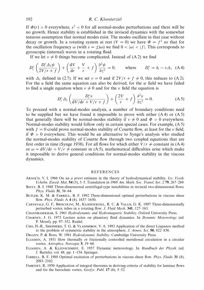
2. Formulation of the linearized problemConsider a steady circular flow or vortex v = V (r) that is in cyclo-geostrophic and

hydrostatic balance:

V 2

r+ f V =

1

ρ

∂P

∂r,

1

ρ

∂P

∂z= −g, (2.1)

where p = P (r, z) is the pressure, ρ is the constant density and g is the gravitationalconstant with gravity aligned with the axis of rotation (along the z-axis as sketchedin figure 1) and f the Coriolis parameter representing the effect of rotationin the dynamics. When the kinematic viscosity ν �= 0, stationary flows mustsatisfy

1

r

d

drrdV

dr− V

r2= 0

(like Couette flow between two concentric cylinders). Nonetheless, when we performa stability analysis below in § 2.3 with viscous effects included, we will treat thebasic state as stationary. Whether this leads to conclusions one can have confidencein, largely depends on whether the time scales of the evolution of the basic flowand those of the perturbations are well separated. One can also envision thepossibility of introducing an appropriate circularly symmetric external force fieldacting in the azimuthal direction which renders the azimuthal v field stationary(see § 5).


Introducing perturbations u, v, w and p independent of the azimuthal angle θ andlinearizing about the balanced state (2.1) we get(

∂

∂t− νΔ1

)u −

(2V

r+ f

)v = − 1

ρ

∂p

∂r, (2.2)(

∂

∂t− νΔ1

)v +

(dV

dr+

V

r+ f

)u = 0, (2.3)(

∂

∂t− νΔ

)w = − 1

ρ

∂p

∂z, (2.4)

∇ · u =1

r

∂(ru)

∂r+

∂w

∂z= 0, (2.5)

where

Δ =1

r

∂

∂rr

∂

∂r+

∂2

∂z2and Δ1 = Δ − 1

r2. (2.6)

In what follows, it will also be useful to write

Δ1 =∂

∂r

1

r

∂

∂rr +

∂2

∂z2. (2.7)

Adding u× (2.2) + w× (2.4) we get

∂

∂t

1

2

(u2 + w2

)−

(2V

r+ f

)uv = −u · ∇p/ρ + ν(uΔ1u + wΔw), (2.8)

where

∇ = er

∂

∂r+ ez

∂

∂z, u = eru + eθv + ezw.

With (2.3) it follows that

u = −(∂v/∂t − νΔ1v)/

(dV

dr+

V

r+ f

)= −(∂v/∂t − νΔ1v)/Q (2.9)

provided that the (absolute) vorticity Q defined in (1.1) vanishes nowhere. There willbe difficulties, for example, if f = 0 and V is potential flow (i.e. V ∝ 1/r), as foundoutside a spinning cylinder which is placed in a large quiescent basin. In that case ouranalysis fails because then Q = 0 so that (2.9) is meaningless. Assuming that Q �= 0everywhere, we can substitute (2.9) in (2.8) and get

∂

∂t

1

2

[u2 + w2 + Fv2

]= −u · ∇p/ρ + ν(uΔ1u + wΔw + FvΔ1v) (2.10)

with F(r) defined in (1.3).

2.1. Inviscid dynamics

If we set ν = 0 and integrate (2.10), we find that

dEdt

= 0 with E =1

2

∫V

[u2 + w2 + Fv2

]dV (2.11)

provided that∫

V div(up/ρ) dV = 0. dV = 2πr dr dz stands for the volume integralover the domain. This will hold if the flow is either enclosed by rigid boundarieswhere u · n = 0 with n the unit vector normal to such boundaries (no flux condition),or can be in a domain unbounded in one or more direction, in which case we require


that u vanishes ‘fast enough’ for r → ∞ if unbounded in the radial direction, or forz → ±∞ if unbounded in the vertical. If there is no interior boundary, things mustof course be ‘well behaved’ at the origin r = 0. From here on we shall call E theeffective energy.

If 2V/r + f �= 0 everywhere the effective energy can also be written as

E =1

2

∫V

[u2 + w2 +

(2V /r + f )2

Φv2

]dV. (2.12)

We mentioned this result (without a derivation) already in Kloosterziel et al. (2007).Clearly E is a positive-definite functional if the inviscid classical condition Φ > 0is satisfied everywhere in the domain because then also F > 0 everywhere. Thisestablishes Lyapunov stability in the inviscid dynamics, i.e. the perturbation energyE, ||u|| ≡ [

∫V u2dV]1/2, ||w|| and ||v|| can be kept arbitrarily small at all times by

choosing the initial perturbations ‘small enough’. To see this, note that if F > 0everywhere, it follows that if at some initial time (say t = 0) small perturbations areintroduced, then at all times (subscripts ‘0’ indicate t = 0)

E(t) = E0 =1

2

∫V

[u2

0 + w20 + Fv2

0

]dV > 0 and (2.13)

0 �1

2

∫V

(u2+w2)dV � E0, 0 �1

2min {F}

∫V

v2dV �1

2

∫V

Fv2dV � E0. (2.14)

The last inequality implies

0 �1

2

∫V

v2dV �E0

min {F} . (2.15)

From here on ‘min{· · · }’ and ‘max{· · · }’ stand for the minimum and maximum of thefunction in the domain. The total perturbation energy E is

E =1

2

∫V

[u2 + w2 + v2

]dV. (2.16)

For convenience we have dropped the constant density ρ here. It easily verified that

0 � E �E0

min {F} if min {F} � 1 and

0 � E � E0 if min {F} � 1.

⎫⎬⎭ (2.17)

Hence E can be kept arbitrarily small if F > 0 everywhere provided that E0 < ∞.Finite E0 is guaranteed if F < ∞ everywhere which means that Q = 0 cannot beallowed.

The perturbation energy evolves according to

dE

dt= −

∫V

[(dV

dr− V

r

)uv

]dV + ν

∫V

(uΔ1u + vΔ1v + wΔw) dV. (2.18)

If the classical criterion for stability (Φ > 0 or F > 0 everywhere) is satisfied andν = 0, clearly one would be hard pressed to establish stability with (2.18). But, (2.17)shows that there will then always be Lyapunov stability.

2.2. Transient growth

Although the perturbation energy can be kept arbitrarily small by taking the initialperturbations u0, v0 and w0 small enough, there can be transient growth dE/dt > 0


for some period of time. Much recent research has focused on finding ‘optimalperturbations’ for a variety of flows that lead to the greatest possible transientamplification of initial perturbations. This transient growth phenomenon can occurin any system where the operators that describe the linearized dynamics are non-normal, i.e. not self-adjoint so that eigenmodes (as in normal-modes analysis) are notmutually orthogonal. Even in systems that are exponentially stable (normal-modesstable), large growth for some finite time-interval is sometimes possible for largeReynolds numbers (see e.g. Farrell 1988, Butler & Farrell 1992, Trefethen et al. 1993,Pradeep & Hussain 2006, Schmidt 2007). An upper bound for the so-called ‘gain’G(t) = E(t)/E0 can be determined as follows: First note that

E0 �1

2

∫V

[u2

0 + w20 + max {F} v2

0

]dV =

1

2

(||u0||2 + ||w0||2 + max {F} ||v0||2

).

(2.19)Next note that

E0

E0

�||u0||2 + ||w0||2 + max {F} ||v0||2

||u0||2 + ||w0||2 + ||v0||2 � max {F} when max {F} � 1,

� 1 when max {F} � 1.

⎫⎪⎬⎪⎭ (2.20)

Dividing both sides of the inequalities in (2.17) by E0 yields with (2.20)

E(t)/E0 = G(t) � Gmax = 1/min {F} when max {F} � 1, (2.21a)

= max {F} when 1 � min {F} , (2.21b)

= max {F} /min {F} when min {F} � 1 � max {F}. (2.21c)

This upper bound Gmax for the gain is valid for any classically stable and thereforeLyapunov stable flow in the inviscid dynamics. If F ≈ 1 everywhere, then Gmax

slightly exceeds unity. If one imagines, for example, that F = 1 (take f = 0 andsolid-body rotation V (r) = Ωr) then E = E and Gmax = 1 according to (2.21c). Thereis neither transient growth nor decay: both dE/dt = 0 and dE/dt = 0.

One may wonder whether these upper bounds are sharp or not. Consider firstthe case 0 < F � 1 so that according to (2.21a) the upper bound is Gmax =1/min {F}. Imagine that initially there are meridional velocity perturbations u0, w0

while v0 = 0. Then E0 = (1/2)(||u0||2 + ||w0||2) = E0. Assume that later the meridionalvelocity perturbations vanish and instead there is a highly concentrated azimuthalperturbation velocity field v centred about the position r = rmin where F(rmin) =min {F} � 1. Then E(t) = (1/2)||v(t)||2 and by conservation of E we have E(t) �(1/2)min {F} ||v(t)||2 = E0 = E0 or E(t) � E0/min {F}. Then E(t)/E0 � 1/min {F}which is (2.21a). Physically this scenario is plausible if the initial u, w fields areconcentrated about rmin. In the inviscid dynamics we expect that the upper bound(2.21a), although unattainable, is quite sharp and that maximum amplification isfound for initial meridional velocity perturbations located in a narrow region whereF(r) attains it minimum.

The upper bound (2.21b) for cases with F � 1 follows likewise by imagining thatinitially there is an azimuthal perturbation field v0 highly concentrated about r = rmax

where F(rmax) = max {F} � 1. If u0 = w0 = 0 we then have E0 = (1/2)||v0||2 andE0 � (1/2)max {F} ||v0||2. If at a later time v = 0 and there are non-zero meridionalvelocity perturbations then E(t) = (1/2)(||u(t)||2 + ||w(t)||2) = E(t). But conservationof E implies E(t) = E(t) � max {F} E0 so that E(t)/E0 � max {F}. This suggests


that the upper bound in (2.21b) could be approached by choosing an initial v fieldthat is confined to a narrow region about r = rmax .

If max {F} > 1 and min {F} < 1, the upper bound Gmax = max {F} /min {F}in (2.21c) is found by imagining that initially there is a v field concentrated in theregion about rmax while u0 = w0 = 0 and that at a later time again u = w = 0 whilethe v field is then concentrated around r = rmin. This is not a plausible scenario:it is unlikely that an initial v field concentrated in one region evolves according to(2.2)–(2.4) towards a v field that is concentrated in a different region. Hence for flowswith min {F} 1 max {F}, Gmax in (2.21c) is probably rather conservative.

2.3. Viscous dynamics

We will now derive criteria for viscous flows that guarantee that E is positive definitewhile at all times dE/dt � 0. With the assumption that we can treat V as stationary,we have

dEdt

= ν

∫V

(uΔ1u + wΔw) dV + ν

∫V

FvΔ1v dV. (2.22)

Again, this is only valid if∫

V div(up/ρ) dV = 0. At boundaries we require theperturbations u, v, w to vanish and in any infinite direction they are again required tovanish rapidly enough. Then (2.22) is valid and through partial integration it followsthat the first term on the right-hand side in (2.22) becomes

ν

∫V

(uΔ1u + wΔw) dV = −ν

∫V

(∣∣r−1∇ru∣∣2 + |∇w|2

)dV, (2.23)

where |a∇b|2 = a2(∂rb)2 + a2(∂zb)2. The term (2.23) would also arise as a part of theusual viscous dissipation of the perturbation energy E. Let us evaluate the secondterm on the right-hand side of (2.22). The part involving the ∂2

z operator in Δ1

simply gives the term ν∫

V Fv∂2z v dV = −ν

∫V F(∂zv)2 dV. The part involving the r

derivatives can be evaluated in two ways, (A) uses the form Δ − 1/r2 with Δ as in(2.6) while (B) uses the r operator as in Δ1 in (2.7). Assuming F to be continuousand twice differentiable, we find through partial integration:

(A)

∫V

Fv

(1

r

∂

∂rr∂v

∂r− v

r2

)dV = −

∫V

F[(

∂v

∂r

)2

+(v

r

)2

]dV

+1

2

∫V

1

r3

d

drrdFdr

(rv)2 dV,

(B)

∫V

Fv∂

∂r

1

r

∂rv

∂rdV = −

∫V

F(

1

r

∂rv

∂r

)2

dV +1

2

∫V

1

r

d

dr

1

r

dFdr

(rv)2 dV.

Thus we get

(A)dEdt

= −ν

∫V

(∣∣r−1∇ru∣∣2 + |∇w|2

)dV − ν

∫V

F |∇v|2 dV

+ν

2

∫V

(d2Fdr2

+1

r

dFdr

− 2Fr2

)v2 dV, (2.24)

(B)dEdt

= −ν

∫V

(∣∣r−1∇ru∣∣2 + |∇w|2

)dV − ν

∫V

F∣∣r−1∇rv

∣∣2 dV

+ν

2

∫V

(d2Fdr2

− 1

r

dFdr

)v2 dV. (2.25)


From this it follows that a sufficient condition for stability is that

F(r) > 0 and (A)d2Fdr2

+1

r

dFdr

− 2Fr2

� 0 or (B)d2Fdr2

− 1

r

dFdr

� 0, (2.26)

because then E = (1/2)∫

V(u2 + w2 + Fv2dV) is positive definite and at all times theright-hand side in (2.24) or (2.25) is negative or zero and thus dE/dt � 0.

But, this can be improved as follows: Consider (2.24)−c×(2.25), with c �= 1 aconstant:

(1 − c)dEdt

= −(1 − c)ν

∫V

{∣∣r−1∇ru∣∣2 + |∇w|2 + F

(∂v

∂z

)2}

dV

+ν

2

∫V

{(1 − c)

d2Fdr2

+ (1 + c)1

r

dFdr

}v2dV

− ν

∫V

F{

(1 − c)

[(∂v

∂r

)2

+(v

r

)2

]− 2c

∂v

∂r

v

r

}dV. (2.27)

The term {· · · } in the last integral on the right-hand side in (2.27) equals

(1 − c)

{(∂v

∂r−

( c

1 − c

) v

r

)2

+

(1 − c2

(1 − c)2

)(v

r

)2

}.

We divide both sides of (2.27) by (1 − c) and set

α =1 + c

1 − cso that 2

(1 − c2

(1 − c)2

)=

1

2(3 − α)(1 + α) and

c

c − 1=

1

2(α − 1).

The effective energy equation then becomes

dEdt

= −ν

∫V

{∣∣r−1∇ru∣∣2+|∇w|2 + F

(∂v

∂z

)2}

dV−ν

∫V

F(

∂v

∂r− 1

2(α − 1)

v

r

)2

dV

+ν

2

∫V

{d2Fdr2

+α

r

dFdr

− 1

2(3 − α)(1 + α)

Fr2

}v2dV. (2.28)

Therefore a sufficient condition for stability of a viscous flow with respect to arbitrarysymmetric perturbations is that, for some constant α, (1.4) is satisfied everywhere. In(1.4) only the range −1 � α � 3 is useful since only in that range (3 − α)(1 + α) � 0.For α = 1 this is condition (A) in (2.26), while (B) is found for α = −1.

Stability also follows if F > 0 and if

1

2

∫V

{d2Fdr2

+α

r

dFdr

− 1

2(3 − α)(1 + α)

Fr2

}v2dV−

∫V

F(

∂v

∂r− 1

2(α − 1)

v

r

)2

dV� 0.

(2.29)If F > 0 we can substitute v = v/

√F in (2.24), (2.25) or (2.28). Then

∂v

∂r=

1

F1/2

∂v

∂r− 1

2

(dF/dr

F3/2

)v,

and if this is substituted in the integral∫

V F |∇v|2 dV that appears in (2.24) one gets∫V

F |∇v|2 dV=

∫V

(∂v

∂z

)2

dV+

∫V

{(∂v

∂r

)2

− v

FdFdr

∂v

∂r+

1

4

(dF/dr

F

)2

v2

}dV.


Next we use that

−∫

V

v

FdFdr

∂v

∂rdV = −1

2

∫V

∂

∂r

(rv2

FdFdr

)drdz +

1

2

∫V

v2

r

d

dr

(r

FdFdr

)dV.

Assuming v and therefore v to vanish at boundaries or rapidly enough for large r orat r = 0, the integral

∫V ∂/∂r (· · · ) dr dz = 0 and we find that (2.24) becomes

dEdt

= −ν

∫V

{∣∣r−1∇ru∣∣2 + |∇w|2 +

(∂v

∂z

)2}

dV

− ν

∫V

{(∂v

∂r

)2

− 1

4

[(dF/dr

F

)2

− 4

r2

]v2

}dV. (2.30)

Equations (2.25) and (2.28) also take this form after the substitution v = v/√

F.Hence stability is also guaranteed if (1.5) holds everywhere. One might expect that(1.5) is a less conservative condition than (1.4) since (1.5) follows from combiningthe second negative-definite integral on the right-hand side of (2.28) with the lastintegral containing G(r; α) which we defined in (1.4). But, as we will see in the nextsection, this is not necessarily true. In any case, if either (1.4) or (1.5) is satisfied,dE/dt = 0 only when ∇ru, ∇w, ∇v and v = 0 everywhere in the domain. If thedomain is either confined in the vertical or in the horizontal by rigid boundarieswhere the perturbations vanish, this implies that u = v = w = 0 so that limt→∞E = 0and limt→∞E = 0. Hence the flow would then be forced back towards the basic flowV (r) and the flow is asymptotically stable.

If either (1.4) or (1.5), or both, are satisfied everywhere, the upper bounds Gmax

on the gain due to possible transient growth remain (2.21a)–(2.21c) because thendE/dt � 0 at all times so that instead of (2.17) we have

0 � E(t) �E(t)

min {F} �E0

min {F} if min {F} � 1,

0 � E(t) � E(t) � E0 if min {F} � 1.

⎫⎬⎭ (2.31)

Division by E0 and using (2.20) then again yields (2.21a)–(2.21c). For small Reynoldsnumbers Re, these upper bounds are expected to be conservative because the evolutionequations (2.28) and (2.30) indicate that the effective energy E will diminish rapidlyfor small Re if either (1.4) and/or (1.5) is satisfied everywhere.

3. Couette flowThe well-known Couette flow of a viscous fluid between rotating coaxial cylinders

has the velocity distribution

V (r) = Ar + B/r with A = Ω1

μ − η2

1 − η2, B = Ω1R

21

1 − μ

1 − η2(3.1)

and the parameters

μ = Ω2/Ω1 and η = R1/R2.

R1 and R2 are the radius of the inner and the outer cylinder which rotate withangular velocity Ω1 and Ω2, respectively (see Drazin & Reid 1981). The Rayleighdiscriminant Φ(r) (with f = 0) is positive throughout the domain R1 � r � R2 if


μ > η2. This means that for classical (inviscid) stability the cylinders must rotate inthe same direction and

|V (R2)R2| > |V (R1)R1|. (3.2)

We have

F(r) = 1 +B

Ar2= 1 +

(1 − μ

μ − η2

)1

(r/R1)2(3.3)

and F(r) > 0 for all r ∈ [R1, R2] if the classical criterion (μ > η2) is satisfied (notethat Φ(r) = 4A2F(r) for Couette flow). Like every flow that satisfies the classicalcondition, in the inviscid dynamics Couette flow is Lyapunov stable.

The second condition in (1.4) is after substitution of (3.3)

G(r; α) = (6 − 2α)B

A

1

r4− 1

2(3 − α)(1 + α)

(1

r2+

B

A

1

r4

)� 0. (3.4)

This will be satisfied for α = 3, i.e. for α = 3 the last term in (2.28) vanishes identicallyfor all r > 0. Hence Couette flow is also Lyapunov stable in the viscous dynamics ifthe inviscid classical criterion is satisfied.

For Couette flow (1.5) is too conservative: we find that the second condition in(1.5) is only satisfied when μ < 2 − η2. This implies that the classical condition plusthe second condition in (1.5) require that the inner and outer cylinder rotate in thesame direction and that

|V (R2)R2| > |V (R1)R1| but |V (R2)R2| < |V (R1)R1|(2(R2/R1)

2 − 1). (3.5)

Thus (1.5) only proves Lyapunov stability of a subset of the classically stable Couetteflows whereas (1.4) proves stability for all classically stable flows. For different flowsthe converse may be true, i.e. (1.5) may sometimes be less restrictive than (1.4). Thisis shown in the next section with an example.

There are two special cases worthwhile mentioning. The first is that of where theinner cylinder is taken out. Then V = Ω2r , which is simply solid-body rotation asfound inside a rotating cylinder after a sufficiently long spin-up time. Then Φ = 4Ω2

2

and F = 1. This is therefore inviscidly stable to symmetric perturbations because theeffective energy is positive-definite, but also Lyapunov stable in the viscous dynamicssince either (2.24) or (2.25) show that dE/dt � 0 and also dE/dt � 0. The secondcase is the limit R2 → ∞ and Ω2 = 0 (μ = 0 and η = 0). The result would be purepotential flow V = Ω1R

21/r outside a spinning cylinder. This has Φ = 0 everywhere

because the vorticity Q is zero and F is undefined. As mentioned in § 2, our approachcannot be used in this case.

4. Lamb–Oseen vortexThe so-called Lamb–Oseen vortex or ‘Gaussian’ vortex has a velocity distribution

V (r) and corresponding vorticity ω given by

V (r) =ω0L

(r/L)

[1 − exp

(−r2/2L2

)], ω(r) =

dV

dr+

V

r= ω0 exp(−r2/2L2). (4.1)

The radius r has been non-dimensionalized with an arbitrary length scale L andω0 is the peak vorticity found at r = 0. V and ω are shown in figure 2(a). UnlikeCouette flow, in a freely evolving viscous fluid this is not a steady state solutionof the Navier–Stokes equations and V and ω evolve according to ∂tV = νΔ1V and


1 2 3 4 50

0.5

1.0

r/L

ω/ω0

V/ω0L

(a) (b)

1 3 4 50

1

2

3

r/L

�

4/(r/L)2

L2 d�/dr�

2

rc/L

Figure 2. (a) The vorticity ω (stippled line) and velocity V (solid line) of the Lamb–Oseenvortex given by (4.1) non-dimensionalized with ω0 and ω0L, respectively, as a function ofr/L. Peak vorticity is ω0 at r = 0 and L is arbitrary. The non-dimensional peak velocityis Vmax/(ω0L) ≈ 0.45 at rmax/L ≈ 1.57. (b) Graph showing F given by (4.2) (thin line),(dF/dr)2/F2 non-dimensionalized with L2 (thick line) and the curve 4/(r/L)2 (stippled line)as a function of r/L. For r > rc/L ≈ 1.79 (indicated by •) the criterion (1.5) is not satisfied.In (a) the symbol • is also shown at the position rc/L.

∂tω = νΔω. If (4.1) defined V and ω at some time t = 0, the time evolution is

V (r, t) =ω0(t)L(t)

(r/L(t))

[1 − exp

(−r2/2L(t)2

)], ω(r, t) = ω0(t) exp

(−r2/2L(t)2

)with

ω0(t) =ω0

1 + 2(νt/L2(0)), L(t) =

√L2(0) + 2νt.

But, we will treat the flow as stationary and only consider V and ω defined in (4.1).

4.1. Non-rotating system

In a non-rotating system (f = 0) the Rayleigh discriminant Φ = 2(V/r) ω > 0 for allr and

F(r) =2V/r

ω= 2

exp(r2/2L2) − 1

(r/L)2� 1 (4.2)

for all r � 0, as shown in figure 3(b). The smallest value F = 1 is found in thelimit r ↓ 0. Thus the effective energy is positive definite. But Lyapunov stability withrespect to symmetric perturbations in the inviscid dynamics cannot be established.The reason is that as r → ∞ we have F → ∞. This is due to the fact that forlarge r the vorticity Q = ω vanishes exponentially fast (the vortex gets ever closer topotential flow V ∝ 1/r so that Q → 0). An upper bound Gmax for the possible gaindue to transient growth in the inviscid dynamics cannot be determined with (2.21b)unless the flow is terminated flow at some finite r = rc. A finite Gmax = F(rc) can becalculated but it can be made arbitrarily large by increasing rc. The fact that Gmax

is not finite on the infinite domain is perhaps not surprising since it is known thatpotential flow can support unbounded algebraic growth (see § 5 for a brief discussion).

For the viscous dynamics we need to determine whether (1.4) or (1.5) can holdeverywhere. In figure 3(b) it is seen that for r/L > rc/L ≈ 1.79 the criterion (1.5) doesnot hold, i.e. the second condition in (1.5) is violated. Between r = 0 and r = rc (1.5)


0 0.5 0.9 1.18 1.5 2.0

0

2

–2

4

r/L α

(a) (b)

α = 2

α = –1

α = 0L2 �

0 1–1 2 30

0.4

0.8

1.2

r c/L

Figure 3. (a) The function G(r; α) given in (1.4) and non-dimensionalized with L2, for theLamb–Oseen vortex and α = −1, 0 and α = 2. For α = −1 and α = 3 (not shown) G � 0 forall r . For α = 0 we have G > 0 for all r/L > rc/L ≈ 1.18. (b) Graph showing the critical radiusrc/L as a function of α ∈ [−1, 3]. The greatest value is found for α ≈ 0.2 with rc/L ≈ 1.19.There are no α values for which G � 0 for all r so (1.4) is never satisfied on the unboundeddomain. The symbol • is at the position r/L = rc/L ≈ 1.79 from figure 3.

is satisfied. If the flow was terminated at r = rc, the flow would be stable but on anunbounded domain Lyapunov stability cannot be established with (1.5).

In figure 3(a) we show G(r; α), defined in (1.4), for a few values of α. In each casethere is a finite value r = rc with G > 0 when r > rc. In figure 3(b) we show thecritical value rc/L as a function of α ∈ [−1, 3]. There are no α values for which (1.4)is satisfied everywhere. Further, the region where (1.4) can be satisfied is confinedto a far smaller range of r values than (1.5): the widest region for which Lyapunovstability can be established according to (1.4) is r/L ∈ [0, 1.19] whereas (1.5) provesstability for the range r/L ∈ [0, 1.79]. On a radially unbounded domain we thereforecannot prove Lyapunov stability.

4.2. Rotating system: cyclones

We now add the Coriolis force to the dynamics (f �= 0) and define the Rossby numberfor the Lamb–Oseen vortex as Ro = ω0/f . If Ro > 0 this is a cyclonic vortex, ifRo < 0 it is an anticyclonic vortex. The Rayleigh discriminant non-dimensionalizedwith f 2 is

Φ(r)/f 2 =(2Ro/(r/L)2

[1 − exp

(−r2/2L2

)]+ 1

) (Ro exp(−r2/2L2) + 1

), (4.3)

while

F =2Ro/(r/L)2

[1 − exp

(−r2/2L2

)]+ 1

Ro exp(−r2/2L2) + 1. (4.4)

For all Ro ∈ (−1, ∞) it can be shown that Φ(r) > 0 for all r (see Carnevale et al.1997). For the cyclone (Ro > 0) this is easily seen with (4.3). Further, for all Ro > −1we find that F > 1/2 for all r � 0. Thus, when Ro > −1 the effective energy ispositive definite and the vortex is therefore Lyapunov stable in the inviscid dynamicsfor all Rossby numbers Ro > −1. The smallest value F = 1/2 is found in the limitRo → −1 and r ↓ 0. The limiting case Ro → −1 is singular in that the absolutevorticity Q = ω + f tends to zero in the limit r ↓ 0 so that F becomes undefinedthere (remember F = (2V/r + f )/Q).

For the viscous dynamics, we first consider the cyclone case Ro > 0. In figure 4(a)we show F for a few positive Rossby numbers. Generally for all Ro > 0 we have


2 4 6 80

1

4

8

r/L

Ro = 10

�

Ro = 50

Roc = 26

(a) (b)

1 2 3 4 50

0.5

1.0

1.5

r/L

Roc = 26

Ro = 50

Ro = 10 4/(r/L)2

L2 d�/dr�

2

Figure 4. (a) F as a function of r/L for the cyclonic Lamb–Oseen vortex withRo = ω0/f = 10, 26 (thick line) and Ro = 50. For any Ro > 0 we have F � 1 for allr � 0. (b) (dF/dr)2/F2 for Ro = 10, 26 and 50 and non-dimensionalized with L2 (solidlines) and the curve 4/(r/L)2 (stippled line) as a function of r/L. For 0 < Ro � Roc ≈ 26the criterion (1.5) is satisfied for all r � 0 (numbers are approximate: 26 < Roc < 26.01). ForRo = Roc the curve L2(dF/dr)2/F2 ‘touches’ the curve 4/(r/L)2 at r/L ≈ 2.25 (thick line).For Ro > 26 there is a range of r values in which the second condition in (1.5) does not hold.For all Ro < 26 the cyclone is Lyapunov stable according to (1.5).

0 1 2 3 4 5−6

−3

0

3

r/L

α = –1

α = 3

α = 0.6Roc = 10

−1.0 0 0.60 1.0 2.0 3.00

1

2

3

max L2�

Roc = 10

Ro = 26r

(a) (b)

L2 �

α

Figure 5. (a) The function G(r; α) given in (1.4) and non-dimensionalized with L2 for thecyclonic Lamb–Oseen vortex with Ro = Roc = 10 and α = −1, 0.6 (thick line) and α = 3. (b)Numerically determined non-dimensional maximum of G for Ro = Roc = 10 and Ro = 26 asa function of α ∈ [−1, 3]. For Ro > Roc = 10 the maximum is positive for all α which meansthat there is always a range of r values where the second condition in (1.4) is violated. Forα ≈ 0.6 the maximum is zero, as shown in (a). For all Ro < Roc there is always an α forwhich G � 0 for all r � 0. According to (1.4) this guarantees Lyapunov stability.

F � 1 for all r . Numerically we find that for 0 < Ro � Roc ≈ 26 the criterion (1.5)is satisfied. This is shown in figure 4(b). For Rossby numbers greater that Roc ≈ 26the second condition in (1.5) is violated for some range of r values (the precise valuelies between 26 and 26.01). Thus, (1.5) establishes Lyapunov stability of the cyclonicLamb–Oseen vortex only in the range Ro ∈ (0, 26) in the viscous dynamics whereasstability is guaranteed for all Ro > 0 in the inviscid dynamics.

The stability criterion (1.4) is satisfied for a smaller range of positive Rossbynumbers, i.e. only for 0 < Ro � 10. In figure 5(a) we show G(r; α) for Ro = Roc ≈ 10and a few values of α as indicated. For α ≈ 0.6 we find that G � 0 for all r . This


0 1 2 3 4 50.50

0.75

1.00

Ro = –0.1

Ro = –0.99

Ro = –0.9999

Ro = –0.5

0 1 2 3

10–2

100

102

Ro = –0.5

Ro = –0.99

4/(r/L)2

�

(a) (b)

r/L r/L

L2 d�/dr�

2

Figure 6. (a) F as a function of r/L for the anticyclonic Lamb–Oseen vortex withRo = ω0/f = −0.9999, −0.9, −1/2 and Ro = −1/10. For all Ro > −1 we find thatF � 1/2 for all r . (b) (dF/dr)2/F2 non-dimensionalized with L2 (solid lines) and the curve4/(r/L)2 (stippled line) as a function of r/L. For −1 < Ro < 0 the criterion (1.5) is satisfiedfor all r � 0. This is illustrated here with the examples Ro = −0.9 (thick line) and Ro = −1/2(thin line). Also for Ro = −0.9999 is L2(dF/dr)2/F2 < 4/(r/L)2 for all r (not shown).

is seen in figure 5(a) where for α = 0.6 G ‘touches’ the zero level at some r betweenr = 1 and r = 2, becomes negative again and then asymptotically G → 0 for r → ∞.In this case with Ro ≈ 10, for all α �= 0.6 we find that G > 0 for some range of r

values. This is illustrated in figure 5(a) with two examples. In figure 5(b) we showmaxr{G} as a function of α. For Ro = Roc ≈ 10 we see that maxr{G} = 0 justfor α ≈ 0.6, while for all other α the maximum is positive. For Ro � 10 we findmaxr{G} > 0 for all α and the second condition in (1.4) can therefore not be satisfiedfor any α when Ro � 10. This is illustrated in figure 5(b) with Ro = 26. For allRossby numbers 0 < Ro < Roc ≈ 10, there is always an α ∈ [−1, 3] for which G � 0for all r (in each case G → 0 as r → ∞). Thus, with (1.5) we find the widest range ofpositive Rossby numbers (0 < Ro � 26) for which we can prove Lyapunov stabilityin the viscous dynamics.

Contrary to the case of the vortex in a non-rotating environment, we can determinethe upper bound on the gain Gmax . Since for any finite positive Rossby number1 � F < ∞, according to (2.21b) we have Gmax = max{F}. Figure 8(a) shows Gmax

as a function of the Rossby number in the (viscously) stable range 0 < Ro � 26. Forthe largest Rossby number Ro = 26 we find that Gmax ≈ 5.25. Since this upper boundis valid for any Reynolds number, including the limit Re → ∞, this is in markedcontrast with the result of Pradeep & Hussain (2006) who studied the Lamb–Oseenvortex in a non-rotating system. They showed that there can be significant transientgrowth of axisymmetric perturbations well outside the core of the vortex. A 100-foldincrease in the total perturbation energy E (a gain G = 102) was found even for amodest Reynolds number Re = 2500, although the flow is normal-modes stable. Thedifference between the rotating and the non-rotating case is further discussed in § 5.

4.3. Rotating system: anticyclones

In the inviscid dynamics the anticyclonic Lamb–Oseen vortex is classically andLyapunov stable for all Rossby numbers in the range −1 < Ro < 0. In figure 6(a) weshow F for a few negative Rossby numbers. For Ro ≈ −1 (illustrated in figure 6a withRo = −0.9999) the smallest possible value F = 1/2 is approached near r = 0. The


0 1 2 3 4 5−1.0

−0.5

0

Ro = –0.99

α = 2.34

α = 1

α = –0.57

−1.0

−0.5

0

Ro = –0.5

α = 2.66

α = 1

α = –0.74(a) (b)L

2 �

r/L0 1 2 3 4 5

r/L

Figure 7. (a) The function G for the anticyclonic Lamb–Oseen vortex with Ro = −0.99 andα values as indicated. For all α ∈ [−0.57, 2.34] we find that G � 0 for all r . For the twobounding values of this range G is shown as a thick line. (b) Same as (a) but for Ro = −1/2and α values as indicated. For all α ∈ [−0.74, 2.66] we have G � 0 for all r . In both casesthe anticyclonic Lamb–Oseen vortex is Lyapunov stable according to (1.4). Generally for anyRossby number −1 < Ro < 0 there is a range of α values within the range [−1, 3] thatyield G � 0 for all r while G → 0 for r → ∞. The narrowest range is found in the limitRo ↓ −1. For Ro = −0.9999 it is to three significant digits the same as shown in (a), i.e. for−0.57 � α � 2.34.

0 5 10 15 20 251

2

3

4

5

Ro

(a) (b)

Gmax

−1.00 −0.75 −0.50 −0.25 01.0

1.5

2.0

Gmax

Ro

Figure 8. Upper bound Gmax for the gain G(t) = E(t)/E(0) for (a) the cyclonic Lamb–Oseenvortex for the Lyapunov stable range of Rossby numbers 0 < Ro � 26 with Gmax = max {F}and (b) for the anticyclonic Lamb–Oseen vortex in the Lyapunov and classically stable range−1 < Ro < 0 with Gmax = 1/min {F}. For Ro = 26 we have Gmax ≈ 5.25 in (a) while forRo ↓ −1 in (b) Gmax → 2. The bounds are valid for any Reynolds number.

second condition in (1.5) is satisfied for all Rossby numbers in the classically stablerange −1 < Ro < 0. This is illustrated in figure 6(b) with the examples Ro = −0.9 andRo = −1/2. A logarithmic scale is used along the vertical axis because of the largedifferences between the peak values of (dF/dr)2/(F)2 as the Rossby number varies.So, contrary to the cyclonic case, (1.5) proves Lyapunov stability of the anticyclonicLamb–Oseen vortex in the viscous dynamics for all Rossby numbers in the classicallystable range.

We find that (1.4) also proves stability for the entire classically stable range: for allRossby numbers in this range (−1 < Ro < 0) there is always an α ∈ [−1, 3] for whichG � 0 for all r . Figure 7 shows two examples: in figure 7(a) the Rossby number isRo = −0.99, in figure 7(b) Ro = −1/2. In both cases there is a negative and positive


α (indicated by the thick lines) for which G = 0 at some finite r . For all α in betweenthese two extremes, G < 0 for all finite r and only asymptotically G → 0 as r → ∞.For Ro = −0.99 Lyapunov stability follows for −0.57 � α � 2.34 (see figure 7a), forRo = −1/2 stability for −0.74 � α � 2.66 (see figure 7b). The smallest range of α

values with which Lyapunov stability follows is found in the limit Ro ↓ −1.The bound Gmax on the gain is shown in figure 8(b). Since 0 < F � 1 in this case,

according to (2.21a) Gmax = 1/min {F}. In the entire range −1 < Ro < 0, Gmax neverexceeds a value of 2. Hence just as in the cyclonic case, no significant transient growthcan be expected for the anticyclonic Lamb–Oseen vortex with Rossby numbers in thestable range, no matter how large the Reynolds number is.

5. Summary and discussionIn this paper we have first shown that if the inviscid classical criterion for symmetric

stability is satisfied (F(r) > 0 or Φ(r) > 0 everywhere), the effective energy E definedin (2.11) or (2.12) is a Lyapunov functional. It establishes Lyapunov stability in theinviscid dynamics for arbitrary circular flows with respect to circularly symmetricperturbations. In the inviscid dynamics dE/dt = 0 and we showed that Gmax in(2.21a)–(2.21c) provides an upper bound for the amplification of perturbation energywhich may occur due to transient non-modal growth in the inviscid dynamics. Thedevelopment is somewhat simpler but otherwise analogous to the case of parallelshear flows in stratified fluids as discussed in Kloosterziel & Carnevale (2007).

Next we have derived two novel criteria for Lyapunov stability of viscous circularflows with respect to symmetric perturbations, i.e. (1.4) and (1.5). In both criteria wefirst find the requirement for classical inviscid stability, i.e. Φ > 0 or F > 0 whichguarantees that E is positive definite. The additional conditions guarantee that in theviscous dynamics dE/dt � 0 at all times. This implies that the upper bound Gmax

for the gain in the inviscid dynamics remains valid for the viscous dynamics. If thesecond conditions in (1.4) and (1.5) are not satisfied in some overlapping regions,there is the possibility that the effective energy grows for some period of time, i.e.E(t) > E0 and then (2.21a)–(2.21c) may not be true.

The theory has been applied to a few examples. For other types of vortices orconfined circular flows than discussed in this paper, one must apply both (1.4) and(1.5) to see if the flow is provable stable. If a flow is characterized by a variableparameter like the Rossby number in rotating systems or some parameter whichdetermines the velocity distribution and is provable stable with both (1.4) and (1.5),the results must be compared to see which of the two criteria proves stability for thebroadest range of the parameter(s). It is impossible to predict a priori.

For Couette flow we established in § 3 with (1.4) Lyapunov stability for the entireclassically stable range by setting α = 3. A normal-modes analysis by Synge (1938)and an energy method by Wood (1964) had already established this, but both studieswere specifically aimed at Couette flow. In this study it quickly followed with thegeneral condition (1.4) which can be applied to any flow for which Q �= 0 everywhere.

In § 4.1 we found it impossible to prove Lyapunov stability of the Lamb–Oseenvortex in a non-rotating system (f = 0), both in the inviscid and the viscous dynamics.For the inviscid case this is not surprising because for large r the Lamb–Oseen vortexapproaches potential flow, i.e. according to (4.1) for large r we have approximatelyV (r) ≈ ω0L

2/r so that Q ≈ 0. As noted by Miyazaki & Hunt (2000), potential flowsupports unbounded algebraic growth. This is easily seen by setting ν = 0 and f = 0in (2.3) so that ∂v/dt = 0 when V ∝ 1/r . Hence for potential flow v(r, z, t) = v0(r, z)


remains unchanged. This can drive growth of the azimuthal vorticity ωθ in thelinearized dynamics according to

∂ωθ

∂t=

∂

∂t

[∂u

∂z− ∂w

∂r

]=

2V

r

∂v0

∂z(5.1)

provided that ∂v0/∂z does not vanish everywhere. Therefore the perturbation kineticenergy can grow without bounds if ∂v0/∂z �= 0. Pradeep & Hussain (2006) alsonoted that in the inviscid case the Lamb–Oseen vortex can experience amplificationof perturbation energy that becomes unbounded as the ‘optimal’ perturbations areinitiated at ever increasing distances from the vortex axis. Our thought experimentin § 2.2, which showed how Gmax = max {F} in (2.21b) might be approached, agreeswith their observation that for initial perturbations concentrated at ever larger r ,an ever increasing gain is expected. In the viscous case, Pradeep & Hussain (2006)calculated a maximal gain of about Gmax = 102 for Re = 2500 which will continue toincrease indefinitely with increasing Reynolds number. With our approach we couldnot establish a finite upper bound for the gain because for large r both (1.4) and (1.5)are not satisfied so that (2.21a)–(2.21c) may be false.

In § 4.2 (1.5) proved stability of the cyclonic Lamb–Oseen vortex in the viscousdynamics for a finite range of positive Rossby numbers 0 < Ro � 26 whereas thereis classical stability for all Ro > 0. With (1.4) stability followed for a smaller rangeof Rossby numbers. For 0 < Ro � 26 we found 1 < Gmax � 5.25. Our results implythat even in the case of rather weak rotation (large positive Ro but Ro < 26 or small‘rotation number’ 1/Ro) a numerical search for significant gain (several orders ofmagnitude) in perturbation energy would be futile no matter how large the Reynoldsnumber is.

For Ro > 26 we do not expect a sudden transition to far larger transient growththan for Ro ≈ 26 because there is no destabilizing mechanism present like the double-diffusive mechanism for baroclinic flows mentioned in the introduction. Since everincreasing Ro can be interpreted as ever weaker rotation, the computations by Pradeep& Hussain (2006) for the non-rotating case suggest that as Ro tends to infinity, forfinite Reynolds numbers the maximum gain gradually approaches some finite valueGmax(Re) and Gmax → ∞ as Re → ∞. For the anticyclonic Lamb–Oseen vortex wefound in § 4.3 that either condition (1.4) or (1.5) established stability in the viscousdynamics for the entire classically stable range −1 < Ro < 0 with 1 < Gmax < 2.

We must note that a study of the evolution of an integral quantity like theeffective energy E cannot predict what kind of perturbations, characterized by spatialstructure and relative amplitudes of the three perturbation velocity components,lead to maximal gain in the perturbation energy E. This can only be determinedwith a numerical search procedure as described by Pradeep & Hussain (2006). Forinviscid flows likely candidates are perturbations concentrated about the maximumor minimum of F but for viscous flows further analysis is required.

The modest upper bounds for the possible gain in the case of the Lamb–Oseenvortex in a rotating environment can be understood with simple model which capturesthe inviscid behaviour. The model equations are

∂u

∂t=

(2V

r+ f

)v,

∂v

∂t= −

(dV

dr+

V

r+ f

)u = −Qu, (5.2)


which follow from (2.2) and (2.3) by ignoring pressure perturbations. If we solve (5.2)for some position (r, z), the general solution is

u(t) = u0 cos(√

Φt)

+ v0

√F sin

(√Φt

), v(t) = v0 cos

(√Φt

)−

u0 sin(√

Φt)

√F

.

(5.3)

If V = 0 and f �= 0 one has F = 1 and Φ = f 2 and (5.3) describes simpleinertial oscillations. The effective energy for this model is conserved, i.e. E(t) =(1/2)

(u2(t) + Fv2(t)

)= (1/2)

(u2

0 + Fv20

)= E0 but the kinetic energy is not unless

F = 1. If one chooses a location where F > 1 and takes u0 = 0, then E0 = (1/2)v20

but at time t = 2/(√

Φπ) we have E(t) = (1/2)Fv20 and the ‘gain’ is therefore F > 1. If

F < 1 a gain of 1/F > 1 is found by taking v0 = 0. This is essentially a mathematicalformulation of our thought experiment at the end of § 2.2 which made it plausiblethat the upper bounds (2.21a) and (2.21b) are fairly sharp in the inviscid dynamics.

A Taylor-series expansion yields

u(t) = u0 + v0

(2V

r+ f

)t − 1

2u0Φt2 + . . . , v(t) = v0 − u0Qt − 1

2v0Φt2 + . . . . (5.4)

The higher order terms (proportional to t3, t4, etc.) vanish in the limit Q → 0 inwhich case also Φ → 0. The algebraic growth for potential flow V ∝ 1/r when f = 0,which means Q = 0, is recovered provided that v0 �= 0. When f �= 0, the u and v

field are coupled through the Coriolis force and generally this leads to oscillatorybehaviour.

For large r in the Lamb–Oseen vortex Q ≈ 0 while F 1 and large amplificationis possible but the growth is very slow because Φ ≈ 0. For the Lamb–Oseen vortexin a rotating environment we have Φ > 0 for all Ro > −1. For the cyclone Φ � f 2

whereas for the anticyclone Φ � f 2(1−|Ro|)2. In the context of the simple model thismeans that for the cyclone the time scale Tmax for the transient amplification is fasterthan 1/f , i.e. Tmax < 1/f and for the anticyclone Tmax < 1/(f (1−|Ro|)). A model withRayleigh damping added to (5.2) has been discussed by Pradeep & Hussain (2006,equation (4.2)). This is a reasonable model for the viscous dynamics. It is clear thatwith damping the maximum gain will be smaller and occur at an earlier time than inthe undamped dynamics. For our simple model this means that if damping is added,the time scale Tmax remains smaller than 1/f for the cyclonic Lamb–Oseen vortexand smaller than 1/(f (1 − |Ro|)) for the anticyclone.

As is quite common in viscous stability studies, we assumed that the basic flowV (r) is stationary in the viscous dynamics. This is true for Couette flow, solid bodyrotation and potential flow but not, for example, for the Lamb–Oseen vortex. Thiswas not mentioned by Pradeep & Hussain (2006) and various others preceding themwith studies of viscous transient growth. If we imagine the presence of a circularlysymmetric force field acting in the azimuthal direction, i.e. a force Fθ (r) = −ρνΔ1V (r)then any flow would be stationary. For such a ‘forced-dissipative’ system, our resultsremain valid. But for freely evolving viscous flows like the unforced Lamb–Oseenvortex, the time-dependence may be important. The time scale of evolution of theLamb–Oseen vortex is Tν = L2/ν, where L is roughly the initial ‘size’ of the vortex(the distance from the axis where V = Vmax; see figure 3a). If we take as the relevanttime scale for the growth of perturbations the transient growth time scale Tmax thenthe assumption of stationarity is valid if Tν/Tmax 1. Using the time scale fromour model for Tmax , we expect transient growth to be much faster than the viscous


evolution of the cyclone when Re Ro while for the anticyclone the model suggestthat it requires Re |Ro|/(1 − |Ro|). For any Rossby number Ro > −1 this canbe satisfied if Re is sufficiently large. The favourable comparison found by Pradeep& Hussain (2006, figure 14) between the numerically determined optimal gains Gmax

and the time scale Tmax and the Gmax and Tmax found with the simple model withRayleigh damping, suggests that at least for large-Reynolds-number flows our resultsare valid.

A discussion of separation of time scales is unnecessary if general criteria can beformulated that guarantee Lyapunov stability in the viscous dynamics for arbitrarytime-dependent barotropic flows V = V (r, t) but this has not yet been accomplished.Another obvious extension of this work is to consider what are the stability criteriafor viscous symmetric stability for stationary baroclinic flows V (r, z) in stratified androtating fluids and non-stationary flows V (r, z, t). Also of considerable interest ingeophysical fluid dynamics is symmetric stability/instability of zonal flows on theequatorial β plane. This was already considered by Kloosterziel & Carnevale (2007)but only for a particularly simple flow. Whether sufficient conditions for viscousLyapunov stability can be found for the above mentioned flows is currently an openquestion.

This material is based upon work supported by the National Science FoundationGrant OCE 07-26866. The author would like to express his gratitude to G. F.Carnevale for carefully reading the manuscript.

Appendix. Normal-modes analysisIf normal-modes solutions of the linear perturbation equations exist, we can

derive the inviscid classical criterion for stability (Φ(r) > 0 everywhere) as follows.Eliminating the pressure perturbation between (2.2) and (2.4) and setting ν = 0, weget the equation for the meridional vorticity component ωθ = ∂zu − ∂rw:

∂

∂t

[∂u

∂z− ∂w

∂r

]−

(2V

r+ f

)∂v

∂z= 0. (A 1)

Continuity (2.5) will be satisfied if we introduce a streamfunction for the motions inthe meridional rz plane: u = ∂ψ/∂z, w = −(1/r)∂rψ/∂r. Differentiating (A 1) withrespect to time and substituting ∂v/∂t from (2.3) with ν = 0, we find

∂2

∂t2

[∂

∂r

1

r

∂rψ

∂r+

∂2ψ

∂z2

]+ Φ

∂2ψ

∂z2= 0. (A 2)

This is a simple case of what meteorologists sometimes call the Eliassen–Sawyerequation (Sawyer 1949; Eliassen 1951).

The normal-modes assumption is that we presume that solutions ψ = estΨ (r, z)exist. For convenience we assume that the flow in the meridional plane is boundedby rigid boundaries (e.g. at z = 0 and z = H and at some radius r = R). The no-fluxcondition is satisfied if we set Ψ = 0 at such boundaries. Ψ may be complex and if soΨ � (� indicates complex conjugate) must also vanish at the boundaries. We replace∂2/∂t2 by s2 in (A 2), ψ by Ψ and then multiply by Ψ �. Integrating over the domainwe find, using the boundary condition for Ψ and Ψ �, that

s2 = −∫

VΦ

∣∣∣∣∂Ψ

∂z

∣∣∣∣2

dV/

∫V

(∣∣∣∣1r ∂Ψ r

∂r

∣∣∣∣2

+

∣∣∣∣∂Ψ

∂z

∣∣∣∣2)

dV. (A 3)


If Φ(r) > 0 everywhere, s2 < 0 for all normal-modes perturbations and there will beno growth. Hence stability is established in the inviscid dynamics with the somewhattenuous assumption that normal modes exist. The modes oscillate in that case withoutdecay or growth. In a rotating system at rest (V = 0) we have Φ = f 2 so that forthe oscillation frequency ω (with s = ±iω) we find 0 < |ω| < |f |. This corresponds togyroscopic (internal) waves in a rotating fluid.

If we let ν �= 0 things become complicated. Instead of (A 2) we find

Dνt

(Dν

t Δ1ψ

2V/r + f

)+

(dV

dr+

V

r+ f

)∂2ψ

∂z2= 0, where Dν

t = ∂t − νΔ1 (A 4)

with Δ1 defined in (2.7). If we set ν = 0 and if 2V/r + f �= 0, this reduces to (A 2).For the u field the same equation can also be derived, for the w field we have failedto find a single equation when ν �= 0 and for the v field the equation is

Dνt Δ1

(Dν

t v

dV/dr + V/r + f

)+

(2V

r+ f

)∂2v

∂z2= 0. (A 5)

To proceed with a normal-modes analysis, a number of boundary conditions needto be supplied but we have found it impossible to prove with either (A 4) or (A 5)that generally there will be normal-modes stability if ν �= 0 and Φ > 0 everywhere.Normal-modes stability would follow only in certain special cases. For example, (A 5)with f = 0 could prove normal-modes stability of Couette flow, at least for the v field,if Φ > 0 everywhere. This would be an alternative to Synge’s analysis who studiedthe normal-modes stability of Couette flow through two coupled equations that arefirst order in time (Synge 1938). For all flows for which either V/r �= constant in (A 4)or ω = dV/dr + V/r �= constant in (A 5), mathematical difficulties arise which makeit impossible to derive general conditions for normal-modes stability in the viscousdynamics.

REFERENCES

Arnol’d, V. I. 1966 On an a priori estimate in the theory of hydrodynamical stability. Izv. Vyssh.Uchebn. Zaved. Mat. 54 (5), 3–5. Translation in 1969 Am. Math. Soc. Transl. Ser. 2 79, 267–269.

Bayly, B. J. 1988 Three-dimensional centrifugal-type instabilities in inviscid two-dimensional flows.Phys. Fluids 31, 56–64.

Butler, K. M. & Farrell, B. F. 1992 Three-dimensional optimal perturbations in viscous shearflow. Phys. Fluids A 4 (8), 1637–1650.

Carnevale, G. F., Briscolini, M., Kloosterziel, R. C. & Vallis, G. K. 1997 Three-dimensionallyperturbed vortex tubes in a rotating flow. J. Fluid Mech. 341, 127–163.

Chandrasekhar, S. 1961 Hydrodynamic and Hydromagnetic Stability. Oxford University Press.

Charney, J. G. 1973 Lecture notes on planetary fluid dynamics. In Dynamic Meteorology (ed.P. Morel), pp. 97–352. Reidel.

Cho, H.-R., Shepherd, T. G. & Vladimirov, V. A. 1993 Application of the direct Liapunov methodto the problem of symmetric stability in the atmosphere. J. Atmos. Sci. 50, 822–836.

Drazin, P. & Reid, W. 1981 Hydrodynamic Stability. Cambridge University Press.

Eliassen, A. 1951 Slow thermally or frictionally controlled meridional circulation in a circularvortex. Astrophys. Norvegia 5, 19–60.

Eliassen, A. & Kleinschmidt, E. 1957 Dynamic meteorology. In Handbuch der Physik (ed.J. Bartels), vol. 48, pp. 1–154. Springer.

Farrell, B. F. 1988 Optimal excitation of perturbations in viscous shear flow. Phys. Fluids 31 (8),2093–2102.

Fjørtoft, R. 1950 Application of integral theorems in deriving criteria of stability for laminar flowsand for the baroclinic vortex. Geofys. Publ. 17 (6), 5–52.


Høiland, E. 1962 Discussion of a hyperbolic equation relating to inertia and gravitational fluidoscillations. Geofys. Publ. 24, 211–227.

Kloosterziel, R. C. & Carnevale, G. F. 2007 Generalized energetics for inertially stable parallelshear flows. J. Fluid Mech. 585, 117–126.

Kloosterziel, R. C., Carnevale, G. F. & Orlandi, P. 2007 Inertial instability in rotating andstratified fluids: barotropic vortices. J. Fluid Mech. 583, 379–412.

Kloosterziel, R. C. & van Heijst, G. J. F. 1991 An experimental study of unstable barotropicvortices in a rotating fluid. J. Fluid Mech. 223, 1–24.

McIntyre, M. E. 1970 Diffusive destabilization of the baroclinic circular vortex. Geophys. FluidDyn. 1, 19–58.

van Mieghem, J. M. 1951 Hydrodynamic instability. In Compendium of Meteorology (ed. T. F.Malone), pp. 434–453. American Meteorological Society.

Miyazaki, T. & Hunt, J. C. R. 2000 Linear and nonlinear interactions between a columnar vortexand external turbulence. J. Fluid Mech. 402, 349–378.

Mu, M., Shepherd, T. G. & Swanson, K. 1996 On nonlinear symmetric stability and the nonlinearsaturation of symmetric instability. J. Atmos. Sci 53, 2918–2923.

Ooyama, K. 1966 On the stability of the baroclinic circular vortex: a sufficient condition forinstability. J. Atmos. Sci. 23, 43–53.

Pradeep, D. S. & Hussain, F. 2006 Transient growth of perturbations in a vortex column. J. Fluid.Mech. 550, 251–288.

Rayleigh, J. W. S. 1916 On the dynamics of revolving fluids. Proc. R. Soc. Lond. A 93, 148–154.

Sawyer, S. J. 1947 Notes on the theory of tropical cyclones. Quart. J. R. Met. Soc. 73, 101–126.

Sawyer, S. J. 1949 The significance of dynamic instability in atmospheric motions. Quart. J. R. Met.Soc. 75, 364–374.

Schmidt, P. J. 2007 Nonmodal stability theory. Ann. Rev. Fluid Mech. 39, 129–162.

Sipp, D. & Jacquin, L. 2000 Three-dimensional centrifugal-type instabilities in inviscid two-dimensional flows in rotating systems. Phys. Fluids A 12, 1740–1748.

Solberg, H. 1936 Le mouvement d’inertie de l’atmosphere stable et son role dans la theorie descyclones. Sixth Assembly, Edinburgh. Union Geodesique et Geophysique Internationale, 66–82.

Synge, J. L. 1938 On the stability of a viscous liquid between rotating coaxial cylinders. Proc. Roy.Soc. A 167, 250–256.

Trefethen, L. N., Trefethen, A. E., Reddy, S. C. & Driscoll, T. A. 1993 Hydrodynamic stabilitywithout eigenvalues. Science 261, 578–584.

Wood, W. W. 1964 Stability of viscous flow between rotating cylinders. ZAMP 15 (3), 313–314.

Yanai, M. & Tokiaka, T. 1969 Axially symmetric meridional motions in the baroclinic circularvortex: a numerical experiment. J. Meteorol. Soc. Japan 47 (3), 183–197.

Viscous symmetric stability of circular ﬂows - SOEST · and their fully nonlinear evolution (see...

Documents

Transcript of Viscous symmetric stability of circular ﬂows - SOEST · and their fully nonlinear evolution (see...