Vol:.(1234567890)

Petroleum Science (2020) 17:768–780https://doi.org/10.1007/s12182-020-00458-6

1 3

ORIGINAL PAPER

Viscous flow simulations through multi‑lobe progressive cavity pumps

F. M. El‑Abd1 · E. M. Wahba1 · I. G. Adam1

Received: 14 July 2019 / Published online: 4 May 2020 © The Author(s) 2020

AbstractComputational fluid dynamics (CFD) simulations of multi-lobe progressive cavity (PC) pumps are limited in the literature due to the geometric complexity of the pump, which places numerous restrictions on the grid generation process. The present study attempts to alleviate such restrictions by developing a detailed numerical procedure for the numerical simulations of multi-lobe progressive cavity pumps. The profile equations for the multi-lobe configuration at any section at each instant of rotation are presented. A structured grid generation method is developed to generate mesh files required for CFD simulations of multi-lobe PC pumps. Results from the present procedure are validated against single-lobe PC pump numerical results available in the literature. Finally, a numerical parametric study is carried out to investigate the effect of the number of lobes, the stator pitch, the circular fillet and clearance on the volumetric efficiency of PC pumps with viscous oils.

Keywords Progressive cavity pump · Structured grid generation · Computational fluid dynamics

List of symbolsC ClearanceE Eccentricity valuedf Fillet circle diameterP PitchRb Base circle radiusrf Fillet circle radiust Timexf, yf Fillet curve coordinatesxm, ym Modified hypocycloid curve coordinatesxp, yp Original hypocycloid curve coordinatesω Angular velocityθL Lobe angle

1 Introduction

Progressive cavity pumps (PCP) are commonly used as an artificial lift device in low pressure wells to enhance oil pro-ductivity. PC pumps use mechanical power from electric motors or sucker rods to lift crude oil from the downhole to

the surface. PCP stators are either made of an elastomer or a metallic material. Elastomer PCP stators are made of rubber, Teflon, silicon or plastic. Internal slip flow of elastomer PCP stators is low compared to metallic PCP stators. Slippage flow rate is a function of pump geometry, differential pres-sure and fluid viscosity (Karthikeshwaran 2014).

Several studies attempted to investigate the performance of PC pumps. A theoretical and experimental investigation was carried out by Vetter and Wirth (1995) on the perfor-mance of single-lobe PC pumps operating with water, which showed that overlapping pumps had more mechanical fric-tion and better volumetric efficiency than pumps with clear-ance. Martin et al. (1999) evaluated the pressure and tem-perature distribution along elastomer single-lobe PC pumps, operating under single-phase and two-phase flow conditions using water and air. At low pressure differences, the maxi-mum pressure was located at an intermediate point along the pump, with this point moving further downstream toward the outlet as the pressure difference increased. They also noticed that the maximum temperature was located at an intermedi-ate location along the pump. Olivet et al. (2002) performed an experimental study on single-phase and two-phase flow within a single-lobe PC pump with a metallic stator, where they found that internal slip was constant along the pump. Gamboa et  al. (2003b) proposed a simplified hydraulic model for single-lobe PC pumps, considering internal defor-mation due to stator material and differential pressure. They obtained the slippage flow across the pump and predicted the

Edited by Xiu-Qiu Peng

* E. M. Wahba emwahba@yahoo.com

1 Mechanical Engineering Department, Faculty of Engineering, Alexandria University, Alexandria, Egypt

769Petroleum Science (2020) 17:768–780

1 3

volumetric efficiency with different operational speeds and pressures. The model showed good agreement with highly viscous oils but failed to predict pump slippage with lower viscosity fluids such as water.

Numerical simulations of PC pumps were carried out by a number of researchers. Gamboa et al. (2003a) pre-sented three simplified models of a PC pump using com-putational fluid dynamics (CFD). However, they concluded that finite element techniques were not suitable for simu-lating the hydrodynamics of PC pumps because of exten-sive grid requirements and the huge number of elements needed to perform such a simulation. Andrade et al. (2010) also reached a similar conclusion, where he stated that the geometric complexity of PC pumps makes the use of CFD as an engineering tool almost impossible. (Paladino et al. 2008, 2011, 2009; Pessoa et al. 2009) presented a three-dimensional CFD model for transient flow in a single-lobe PC pump. The numerical simulations were carried out using ANSYS-CFX. and mesh generation and mesh motion were developed through FORTRAN user-specific routines. The developed model was capable of precisely predicting the volumetric efficiency and viscous losses. Mrinal et al. (2016) developed a three-dimensional CFD model using ANSYS Fluent to predict the flow variables at different operating conditions for PC pumps. The dynamic mesh model in ANSYS Fluent was used for the rotor mesh movement, and the hypocycloid path of the rotor was defined using a user-defined function written in C language. The mesh defor-mation was carried out with spring-based smoothing and local remeshing technique. Numerical simulations for mul-tiphase flow in PC pumps were also reported by de Azevedo et al. (2016). Moreover, Nguyen et al. (2014) used a vector approach and the hypocycloid theory to derive a modified hypocycloid curve which is capable of constructing the pro-file of the PC pump and predicting the flow area between the rotor and stator for any number of lobes. Nguyen et al. (2016) developed a model for predicting an actual multi-lobe PCP performance. The proposed model is a combination of two existing models in the literature, namely an analytical model to predict the theoretical pump performance and a slippage model. Al-Safran et al. (2017) developed a set of theoretical operational, fluid property and pump geometry dimensionless groups that govern fluid flow behavior in a PC pump. Zheng et al. (2018) developed an analytical model for the flow in the metallic stator PCP. Based on the analysis of the meshing movement and the geometry clearance, the slip-page through the transversal and longitudinal sealing regions is calculated considering different slippage mechanisms.

As can be seen from the above literature, CFD simula-tions in PC pumps are fairly limited due to the geometric complexity of the pump. Such complexity results in numer-ous problems in the grid generation process. Moreover, CFD simulations were also limited to single-lobe PC pumps, with

few attempts made to simulate the flow through multi-lobe PC pumps. The present study attempts to address these restrictions in the CFD simulations of PC pumps. In this paper, the PC pump profile equations for any number of lobes are detailed taking into consideration twisting, eccen-tricity, rotational velocity and clearance effects. A struc-tured grid generation method is developed to generate mesh files required for CFD simulations of multi-lobe PC pumps. Results from the present procedure are validated against the single-lobe PC pump results of (Paladino et al. 2008, 2011; Pessoa et al. 2009) and then are extended to the numerical simulation of multi-lobe PC pumps. Finally, a numerical parametric study is carried out to investigate the effect of the number of lobes, the stator pitch, the circular fillet and clearance effects on the volumetric efficiency of PC pumps with viscous oils.

2 PC pump geometry and structured grid generation

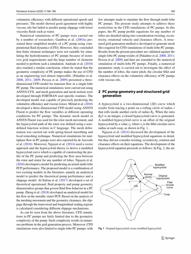
A hypocycloid is a two-dimensional (2D) curve which results from tracing a point on a rolling circle of radius r that rolls inside another circle of radius Rb. When the ratio Rb/r is an integer, a closed hypocycloid curve is generated. A modified hypocycloid curve is an offset of the original hypocycloid by a value rf, where rf is the fillet circular curve radius at each cusp, as shown in Fig. 1.

Nguyen et al. (2014) discussed the development of the hypocycloid and modified hypocycloid equations in detail, but they did not consider twisting, eccentricity, rotation and clearance effects on their equations. The development of the hypocycloid equation proceeds as follows: In Fig. 2, the arc

Modifiedhypocycloid

Originalhypocycloid

rf

Filletcircularcurve

Cusp

NormalvectorTangent

vectory

x

r(θ)

Fig. 1 Original hypocycloid versus modified hypocycloid

770 Petroleum Science (2020) 17:768–780

1 3

length, in red, on the base circle equals the arc length, in blue, on the rolling circle; hence,

where θ is the rolling angle of small circle inside the base circle, N is the ratio between the radius of the base circle and the radius of the rolling circle, N = Rb/r, and ∅ = Nθ. The locus of the tracing point p gives the hypocycloid curve equations as follows:

On the other hand, the modified hypocycloid equations were given by Nguyen et al. (2014) as follows:

where

(1)R� = r�

(2)xp = r(N − 1) cos � + r cos ((N − 1)�)

(3)yp = r(N − 1) sin � − r sin ((N − 1)�)

(4)

xm = r�

(N − 1) cos �1 + cos �2�

+cos �1 − cos �2√

2[1 − cos (N�)]rf

(5)

ym = r�

(N − 1) sin �1 − sin �2�

+sin �1 − sin �2

√

2[1 − cos (N�)]rf

(6)�1 = �

In the modified hypocycloid equations, the normal hypo-cycloid curve is shifted outward in the direction of the unit normal vector with an offset value rf. The fillet curve, as shown in Fig. 1, is part of a circle which has its center located at the cusp point. The fillet curve equation can be expressed as

2.1 Effect of twist

For PC pumps, the rotor and stator geometries are twisted in the three-dimensional (3D) domain. Figure 2 shows the position of the tracing point p in the axial plane, z = 0. At another axial plane z, Fig. 3 shows that point p is shifted by a twisting angle θz. The value of θz depends on the axial position z and the twisting pitch P:

Figure 3 also shows that the radial position of the rolling circle center C1 with respect to base circle center O is r(N-1) and its angle is θ + θz. Moreover, the radial position of point p with respect to the rolling circle center C1 is r with

(7)�2 = (N − 1)�

(8)xf = r[

(N − 1) cos �L + cos �L]

+ rf cos �

(9)yf = r[

(N − 1) sin �L − sin �L]

+ rf sin �

(10)�z = 2�z

P

Base circleRb

Rolling circler

θ

Φ

θ

Rolling circlecenter path

(Rb-r )

P

P0

O

C1

Fig. 2 Hypocycloid curve derivation

Base circleRb

θz

θ

Φ

θz

θ

Rolling circler

Rolling circlecenter path

(Rb - r )

P0

P

C1

O

θz

Fig. 3 Twisting effect on profile equations

771Petroleum Science (2020) 17:768–780

1 3

an angle 2π − ∅ + θ + θz. Hence, taking into consideration the effect of twist, the coordinates of point p for the normal hypocycloid equations become

2.2 Effect of eccentricity

The previous equations describe the stator only, but cannot be directly applied to the rotor due to its eccentric motion with respect to the stator. The eccentricity effect is shown in Fig. 4, where the rotor center C1 is shifted from the stator center O by the distance E . The radial position of rolling circle center C2 with respect to the rotor center C1 is r(Nr − 1) with an angle θz + θ. Moreover, the radial position of point p with respect to the rolling circle center C2 is r and its angle is 2π − ∅ + θ + θz. It is important to note here that the eccentricity has the same value of the rolling circle radius:

2.3 Effect of rotation

The rotor base circle rolls on the stator base circle. Similar to internal gears, the rolling action causes it to rotate around its center and also around the stator’s center. To analyze

(11)xp = r(N − 1) cos(

� + �z)

+ r cos(

(N − 1)� − �z)

(12)yp = r(N − 1) sin(

� + �z)

− r sin(

(N − 1)� − �z)

(13)E = r

the effect of rotation, the motion is divided into two steps: rotation around the stator’s center, as shown in Fig. 5, and rolling on the stator’s perimeter, as shown in Fig. 6. After time t and with the rotor rotating with an angular speed � in the positive counterclockwise direction, the new position of the rotor center will be at an angle �t.

Stator base circleRbs

θz

θ

θ+θz

Φ

Rolling cirlcer

Rotor base circleRbr

E

Rolling circlecenter path

(Rb )

x

y

P P0

C2

O C1

-r

Fig. 4 Eccentricity effect on rotor base circle

Rotor base circleRbr

θ

Φ

Stator base circleRbs

E

θz

θ+θz +w

t

wt

Rolling circlecenter path

(Rbr )

C2

P0

C1

O

P

wt

-r

Fig. 5 Rotational effect on rotor base circle

RotorbasecircleRbr

StatorbasecircleRbs

Φ

E

θz

θ

wt

θ+θz +w

t -Φ2

θ2

PP0

Rolling circlecenter path

(Rb )-r

Fig. 6 Rolling effect on rotor base circle

772 Petroleum Science (2020) 17:768–780

1 3

2.4 Effect of rolling

The rolling direction of the rotor is in the clockwise direc-tion. In Fig. 6, the rotor base circle rolls with an angle ∅2 around the rotor center, such that Rbs ωt = Rbr ∅2. By sim-plifying, we obtain

A summary of the radii and angles of all points is given in Table 1, taking into consideration the combined effects of twist, eccentricity, rotation and rolling. As such, the nor-mal hypocycloid equations after taking all such effects into consideration are expressed as follows:

2.5 Effect of clearance

Industrial PC pumps with a metallic stator maintain a clear-ance between the rotor and the stator (Karthikeshwaran 2014). This clearance could be added to the stator profile or subtracted from the rotor profile. In the modified hypocy-cloid equations, the clearance c is subtracted from the offset value rf.

2.6 PC pump profile equations

Taking into consideration the effects of twist, eccentricity, rotation, rolling and clearance, the modified hypocycloid equations are expressed as follows:

(14)�2 =Rbs

Rbr

�t =Ns

Nr

�t =Nr + 1

Nr

�t

(15)

xp =E cos (�t) + r(

Nr − 1)

cos

(

� + �z−

�t

Nr

)

+ r cos

(

(

Nr − 1)

� − �z+

�t

Nr

)

(16)

yp =E sin (�t) + r(

Nr − 1)

sin

(

� + �z −�t

Nr

)

− r sin

(

(

Nr − 1)

� − �z +�t

Nr

)

Moreover, the fillet circular curve center is located at the cusp points, where the equations at each cusp are given as

It should be noted here that the fillet circular curve is not an exact half-circle. The intersection points could be obtained by simultaneously solving the hypocycloid curve equations with the fillet circular curve equations, which is carried out using a trial-and-error approach in the present study. Equations (17, 18, 21, 22) are also used to describe the stator profile by substituting E = 0 and ω = 0.

2.7 Structured grid generation

Dynamic meshing and structured grid generation for PC pumps are a very difficult and complex process, with the degree of complexity increasing with the increase in the number of lobes. In the present section, we attempt to develop a detailed procedure for generating structured grids for multi-lobe PC pumps.

Equations (17, 18, 21, 22) are used to plot the rotor and stator profiles at each angle of rotation for all longitudinal sections of the PC pump. Radial gridlines are constructed as lines representing angular divisions passing through the stator’s origin and extending from the rotor surface to the stator surface, as shown in Fig. 7. Each radial gridline is then divided to a number of divisions which may be equally

(17)

xm =E cos (�t) + r�

(N − 1) cos �1 + cos �2�

+cos �1 − cos �2√

2(1 − cos (N�))

�

rf − c�

(18)

ym =E sin (�t) + r�

(N − 1) sin �1 − sin �2�

+sin �1 − sin �2

√

2(1 − cos (N�))

�

rf − c�

(19)�1 = � + �z −�t

Nr

(20)�2 =(

Nr − 1)

� − �z +�t

Nr

(21)

xf =E cos (�t) + r(N − 1) cos

(

�L + �z−

�t

Nr

)

+ r cos

(

(

Nr − 1)

�L − �z+

�t

Nr

)

+ rf cos �

(22)

yf =E sin (�t) + r(N − 1) sin

(

�L + �z −�t

Nr

)

− r sin

(

(

Nr − 1)

�L − �z +�t

Nr

)

+ rf sin �

Table 1 Radii and angles including the effects of twist, eccentricity, rotation and rolling

Point Radius Angle

C1 relative to O E wt

C2 relative to C1 r(

Nr − 1)

� + �z + wt − �2

p relative to C2 r 2� − � + � + �z + wt − �2

773Petroleum Science (2020) 17:768–780

1 3

or unequally spaced as shown in Figs. 8 and 9, respectively, for a 5:6 PC pump configuration. Unequally spaced divi-sions would help to accurately resolve the boundary layers at the rotor and stator surfaces. For equal spacing, the point coordinates are computed as follows:

where JN represents the number of grid points along each radial gridline, and i, j, k represent the indices for the angu-lar, radial and axial divisions, respectively. For unequal spac-ing, the hyperbolic tangent stretching approach reported by Paladino et al. (2011) is implemented. After computing the radial and angular divisions for the first axial section (k = 1), the same procedure is repeated for the following longitudinal section. The present structured grid generation procedure is repeated at each time step through one complete revolu-tion of the rotor and for all longitudinal sections of the PC pump. Specification of mesh topology and connectivity and imposition of mesh motion followed the same procedure of Paladino et al. (2011). Generation of a single mesh frame required 9 min on an Intel Core i7 machine with 32-GB RAM. A mesh with 201 radial gridlines is divided into 11

(23)Δx =x(

i, JN , k)

− x(i, 1, k)

JN − 1

(24)Δy =y(

i, JN , k)

− y(i, 1, k)

JN − 1

(25)x(i, j, k) = x(i, 1, k) + (j − 1)Δx

(26)y(i, j, k) = y(i, 1, k) + (j − 1)Δy

unequally spaced divisions and consists of 101 longitudinal sections.

2.8 Governing equations and numerical methods

Fluid flow through multi-lobe progressive cavity pumps is gov-erned by the unsteady form of the Navier–Stokes equations which could be expressed, in standard notation, as follows:

(27)�uj

�xj= 0

(28)�ui

�t+

�(

uiuj)

�xj= −

1

�

�p

�xi+

1

�

�

�xi

[

�

(

�ui

�xj+

�uj

�xi

)]

Stator profile

Radial gridlines

Rotor profile

Fig. 7 Radial gridlines for 3:4 PC pump

Fig. 8 Equally spaced radial gridline divisions for 5:6 PC pump

Fig. 9 Unequally spaced radial gridline divisions for 5:6 PC pump

774 Petroleum Science (2020) 17:768–780

1 3

The commercial software package ANSYS-CFX (Ansys 2016) is used to numerically solve the Navier–Stokes equa-tions. ANSYS-CFX applies a hybrid finite element/finite volume approach for the discretization of the governing equations, where the finite volume method enforces local conservation over each control volume, and the finite ele-ment method is implemented to describe the solution varia-tion within each element to allow for the computation of the required surface fluxes for this element. The high-resolution advection scheme (Nguyen et al. 2016) is applied for the dis-cretization of the convection terms, where it is the second-order accuracy in regions of low gradients and reverts to the first-order accuracy in regions where the gradients sharply change. Implicit second-order accurate time integration is applied in the present study. Fixed time steps are defined to interrupt the solver and continuously replace the mesh frames obtained from the present structured grid generation procedure. Interpolation is carried out to transfer the results from the old mesh frame to the new one at each time instant.

Moreover, the implemented boundary conditions are shown in Fig. 10. Pressure opening boundary conditions are defined at the inlet and outlet, where the inlet pressure is kept at zero pressure and the outlet pressure is varied in order to obtain the pump performance curve.

3 Verification and validation of the numerical procedure

To validate the developed numerical procedure, present results are compared against the CFD results of Paladino et al. (2011) for single-phase flow through a single-lobe PC pump with a rigid stator. The single-lobe PC pump geomet-ric parameters are given in Table 2. Two types of oils were used in Paladino et al. (2011); the first type has a dynamic viscosity of 0.042 Pa s and a density of 868 kg/m3, while the second type has a dynamic viscosity of 0.481 Pa s and a den-sity of 885 kg/m3. For both types of oils, the flow through the PC pump is laminar. The developed structured grid con-sists of 201 radial gridlines divided into 11 unequally spaced divisions to provide better resolution of the boundary layers. In the axial direction, the structured grid consists of 101 longitudinal sections.

Figures 11 and 12 show the performance curve of the single-lobe PC pump using the two types of oils. The

Outlet:Opening

(i.e 40 psi)

Inlet:Opening

(0 psi)Stator: W

all

Rotor: Wall

Fig. 10 Boundary conditions of single-lobe PCP

Table 2 Single-lobe PC pump used for validation

No of lobes 1:2

Eccentricity, mm 4.039Rotor diameter, mm 39.878Stator diameter, mm 40.248Gap, mm 0.185Stator pitch, mm 119.990Number of stages 3

775Petroleum Science (2020) 17:768–780

1 3

performance curve is given in terms of the volumetric flow rate versus the pressure difference at various rotational speeds. As can be seen from both figures, present results are in good agreement with the numerical results of Paladino et al. (2011) and the experimental data of Gamboa et al. (2003a). It is interesting to note here that the slight increase in discrepancy between the experimental and numerical results at higher rotational speeds is due to the need for a

finer time step in the numerical procedure to better resolve such higher rotational speeds.

Verification of the numerical procedure is carried out next for the multi-lobe configurations. Eight different multi-lobe configurations, as shown in Figs. 13 and 14, are considered in the present numerical parametric study, and their geomet-ric parameters are summarized in Table 3. To ensure that the present results are mesh independent, a mesh sensitivity study is carried out on the most complicated configuration, which is the 5:6 lobe configuration. Numerical simulations are performed using four different grids, as shown in Fig. 15, and compared with the theoretical flow rate predicted from Nguyen et al. (2014). Figure 15 shows that doubling the number of elements of the (201 × 11 × 101) grid results in a discrepancy in the predicted flow rate of less than 4%. Moreover, Fig. 15 shows that present numerical predictions are in good agreement with the theoretical flow rate, with a discrepancy of about 11%. Similar mesh sensitivity stud-ies were carried out for the other configurations, providing confidence that the numerical results of the (201 × 11 × 101) grid are mesh independent.

4 Results and discussion

With increasing the number of lobes, it is found that the flow is repeated within a single revolution where the number of cycles is equal to the number of stator lobes as shown in Fig. 16. Therefore, there is no need to perform the simula-tion for a full revolution, only half a revolution would suf-fice for a 1:2 configuration and a one-third revolution for a 2:3 configuration and so on. It should be noted here that such a procedure would not be valid for low-viscosity fluids where inertial terms are important, as for such fluids there is a time for the flow establishment to reach the periodic transient condition. Moreover, Fig. 16 shows that increas-ing the number of lobes results in reduced fluctuations in the flow rate and hence a lower pulsating action in the PC pump performance.

0

10

20

30

40

50

60

0 50 100 150 200

Q, m

3 /day

Differential pressure (PSI)

Current workPaladino et al. (2011)Gamboa et al. (2002)

100 rpm

300 rpm

400 rpm

200 rpm

Fig. 11 Volumetric flow rate versus differential pressure � = 0.481 Pa s

0

5

10

15

20

25

30

35

40

45

50

0 50 100 150 200

Differential pressure (PSI)

Current workPaladino et al. (2011)Gamboa et al. (2002)

100 rpm

300 rpm

400 rpm

200 rpm

Q, m

3 /day

Fig. 12 Volumetric flow rate versus differential pressure μ = 0.042 Pa s

2:3 Lobes (model 2) 3:4 Lobes (model 3) 4:5 Lobes (model 4) 5:6 Lobes (model 5)

Fig. 13 Multi-lobes mesh cross section

776 Petroleum Science (2020) 17:768–780

1 3

(d) (e)

(a) (b) (c)

1:2 Lobes 2:3 Lobes 3:4 Lobes

5:6 Lobes4:5 Lobes

Fig. 14 Cavity shape of different number of lobes

Table 3 Multi-lobe PC pump models

Model no. 1 2 3 4 5 6 7 8

Lobes 1:2 2:3 3:4 4:5 5:6 4:5 4:5 4:5Gap, mm 0.185 0.185 0.185 0.185 0.185 0.050 0.050 0.050Pitch, mm 120 120 120 120 120 120 240 240df, mm 40.248 18.2003 9.9657 9.9657 9.9657 9.9657 9.9657 14.94855E, mm 4.039 6.3673 5.8048 4.6438 3.8699 4.6438 4.6438 4.15Area, mm2 673 708 646 585 525 589 589 570

15.5

16.0

16.5

17.0

17.5

18.0

18.5

200,000 250,000 300,000 350,000 400,000 450,000 500,000

Flow

rate

, m3 /d

ay

Number of nodes

Lobes = 5:6 Speed = 200 rpm ∆P = 0 PSI µ = 0.481 Pa·s

201×11×1

201×11×201

201×21×101

201×16×151

Theoritical flow rate

Fig. 15 Mesh sensitivity study for the 5:6 lobe configuration (model 5)

0

5

10

15

20

0 50 100 150 200 250 300 350

Flow

rate

, m3 /d

ay

Degrees of revolution

1:2 Lobe (Model 1) 2:3 Lobes (model 2)3:4 Lobes (Model 3) 4:5 Lobes (Model 4)

25

Fig. 16 Flow rate at each degree of revolution for different lobes at 200 rpm and 40 psi with viscous oil 0.481 Pa s

777Petroleum Science (2020) 17:768–780

1 3

0

5

10

15

20

25

0 20 40 60 80 100 120 140

Q, m

3 /day

Differential pressure (PSI)

2:3 Lobes (model 2)3:4 Lobes (model 3)4:5 Lobe (model 4)5:6 Lobes (model 5)

Fig. 17 Flow rate versus differential pressure for different lobe con-figurations at 200 rpm

0

5

10

15

20

25

30

35

40

0 20 40 60 80 100 120 140 160 180 200

Q, m

3 /day

Differential pressure (PSI)

2:3 Lobes (model 2)3:4 Lobes (model 3)4:5 Lobe (model 4)5:6 Lobes (model 5)

Fig. 18 Flow rate versus differential pressure for different lobe con-figurations at 300 rpm

0

5

10

15

20

25

30

0 20 40 60 80 100 120 140 160 180 200

Q, m

3 /day

Differential pressure (PSI)

4:5 Lobes (model 6)4:5 Lobe (model 4)4:5 Lobes (model 6)4:5 Lobe (model 4)

300 rpm

200 rpm

200 rpm

300 rpm

Fig. 19 Effect of decreasing clearance on the multi-lobe pump perfor-mance

0

10

20

30

40

50

60

70

0 20 40 60 80 100 120 140 160 180 200

Q, m

3 /day

Differential pressure (PSI)

4:5 Lobes (model 7)4:5 Lobes (model 6)

4:5 Lobes (model 7)4:5 Lobes (model 6)

300 rpm

200 rpm

200 rpm

300 rpm

Fig. 20 Effect of increasing stator pitch on the multi-lobe pump per-formance

30

35

40

45

50

55

60

65

70

0 20 40 60 80 100 120 140 160 180 200

Q, m

3 /day

Differential pressure (PSI)

4:5 Lobes (model 8)4:5 Lobes (model 7)4:5 Lobes (model 8)4:5 Lobes (model 7)

200 rpm

300 rpm

Fig. 21 Effect of increasing fillet diameter on the multi-lobe pump performance

20

30

40

50

60

70

80

90

100

0 20 40 60 80 100 120

Volu

met

ric e

ffici

ency

, %

Differential pressure (PSI)

1:2 Lobes (model 1)2:3 Lobes (model 2)3:4 Lobes (model 3)4:5 Lobes (model 4)5:6 Lobes (model 5)4:5 Lobes (model 6)4:5 Lobes (model 7)4:5 Lobes (model 8)

Fig. 22 Volumetric efficiency of multi-lobe PC pump models at 200 rpm

778 Petroleum Science (2020) 17:768–780

1 3

For the same stator major diameter and same pitch, Figs. 17 and 18 show that increasing the number of lobes would decrease the flow area which, in turn, would reduce the flow rate at the same rotating speed and differential pres-sure. Volumetric efficiency also drops with increasing the number of lobes as they would increase the number of cavi-ties and hence increase the number of sealing lines as shown in Fig. 14, which allows more fluid to escape.

Figure 19 shows that PC pumps with smaller gap have less slip flow, as can be seen from the comparison between models 4 and 6. Moreover, Fig. 20 shows that doubling the stator pitch not only doubles the flow rate but also enhances the volumetric efficiency, as can be seen from the com-parison between models 6 and 7. An interesting geomet-ric parameter is the radius of the fillet curve. Although it slightly reduced the flow area, however, it delivered more flow, as shown in Fig. 21, because of the increased sealing line width which improves sealing and enhances the volu-metric efficiency. Figures 22 and 23 show a comparison of the volumetric efficiency of the different models at 200 rpm and 300 rpm, respectively.

Finally, more physical insight could be gained by con-sidering local flow solutions within the PC pump. As such, Fig. 24 shows the 2:3 lobe configuration (model 2), where six points are selected to monitor flow pressure. The six points are distributed over the stator wall at the major and minor diameters and are located at an axial plane shifted from the inlet by 40 mm, which represents one-third of the stator pitch. Figure 25 shows the pressure at each of the six points as a function of the angle of rotor rotation. All points located on the major diameter show consistent values of pressure with a shifting angle. A similar behavior is also encountered with all points located on the minor diameter. It is interesting to note here the high pressure drop that is encountered when the angle of rotor rotation corresponds to a small gap between the stator and the rotor. Finally, Fig. 26 shows detailed stator pressure contours at different degrees of rotation for the 2:3 lobe configuration (model 2). The pressure contours are provided for every 30° of rotation to clearly demonstrate the progress of the cavity and the liquid pressurization process.

20

30

40

50

60

70

80

90

100

0 20 40 60 80 100

Differential pressure (PSI)

1:2 Lobes (model 1)2:3 Lobes (model 2)3:4 Lobes (model 3)4:5 Lobes (model 4)5:6 Lobes (model 5)4:5 Lobes (model 6)4:5 Lobe (model 7)4:5 Lobes (model 8)

Volu

met

ric e

ffici

ency

, %

Fig. 23 Volumetric efficiency of multi-lobe PC pump models at 300 rpm

Point 1

Point 2

Point 3

Point 4

Point 5

Point 6

Fig. 24 Point distribution in an internal plane of the 2:3 lobe configuration (model 2)

-10

0

10

20

30

40

50

60

0 100 200 300

PS

I

Deg

2:3 Lobe (model 2)Speed = 300 rpmµ = 0.481 Pa·s∆p = 40 PSI

Point 1Point 2

Point 3Point 4

Point 5Point 6

Fig. 25 Local pressure versus angle of rotor rotation for the 2:3 lobe configuration (model 2)

779Petroleum Science (2020) 17:768–780

1 3

5 Conclusions

A detailed structured grid generation procedure is devel-oped in the present study to allow efficient numerical simula-tions of viscous flow through multi-lobe progressive cavity pumps. Effects of twist, eccentricity, rotation and clearance are taken into consideration through the modified hypocy-cloid equations. Present numerical results show that increas-ing the number of lobes results in reduced fluctuations in the flow rate and hence a lower pulsating action in the PC pump

performance. However, volumetric efficiency for multi-lobe PC pumps is shown to drop with increasing the number of lobes, as this would increase the number of cavities and hence increase the number of sealing lines, which allows more fluid to escape.

Open Access This article is licensed under a Creative Commons Attri-bution 4.0 International License, which permits use, sharing, adapta-tion, distribution and reproduction in any medium or format, as long as you give appropriate credit to the original author(s) and the source, provide a link to the Creative Commons licence, and indicate if changes

270° 300° 330°

180° 210° 240°

90° 120° 150°

0° 30° 60°

Fig. 26 Pressure contours for the 2:3 lobe configuration at different degrees of rotation

780 Petroleum Science (2020) 17:768–780

1 3

were made. The images or other third party material in this article are included in the article’s Creative Commons licence, unless indicated otherwise in a credit line to the material. If material is not included in the article’s Creative Commons licence and your intended use is not permitted by statutory regulation or exceeds the permitted use, you will need to obtain permission directly from the copyright holder. To view a copy of this licence, visit http://creat iveco mmons .org/licen ses/by/4.0/.

References

Al-Safran E, Aql A, Nguyen T. Analysis and prediction of fluid flow behavior in progressing cavity pumps. ASME J Fluids Eng. 2017;139(12):121102. https ://doi.org/10.1115/1.40370 57.

Andrade SF, Valerio JV, Carvalho MS. Asymptotic approach for modelling progressive cavity pumps performance. Mec Comput. 2010;XXIX:8429–45.

Ansys Inc. ANSYS CFX-Solver Modeling Guide. 2016.de Azevedo VW, de Lima JA, Paladino E. A 3D transient model

for the multiphase flow in a progressing-cavity pump. SPE J. 2016;21(4):1458–69. https ://doi.org/10.2118/17892 4-PA.

Gamboa J, Olivet A, Iglesias J, Gonzalez P. Understanding the Perfor-mance of a Progressive Cavity Pump with a Metallic Stator. In: Proceedings of twentieth international pump users symposium, Texas A&M University, USA; 2003. https ://doi.org/10.21423 /R12Q3 8.

Gamboa J, Olivet A, Espin S. New approach for modeling progressive cavity pumps performance. SPE annual technical conference and exhibition, Denver, Colorado, USA; 2003. 10.2118/84137-MS.

Karthikeshwaran R. Progressive cavity pump: a review. Biosci Biotech-nol Res Asia. 2014;11:231–7. https ://doi.org/10.13005 /bbra/1415.

Martin AM, Kenyery F, Tremante A. Experimental study of two phase pumping in progressive cavity pumps. Latin American and Car-ibbean petroleum engineering conference, Caracas, Venezuela; 1999. https ://doi.org/10.2118/53967 -MS.

Mrinal KR, Siddique M, Samad A. A transient 3D CFD model of a pro-gressive cavity pump. ASME turbo expo 2016: turbomachinery

technical conference and exposition, Seoul, South Korea; 2016. https ://doi.org/10.1115/GT201 6-56599 .

Nguyen T, Al-Safran E, Saasen A, Nes OM. Modeling the design and performance of progressing cavity pump using 3-D vec-tor approach. J Pet Sci Eng. 2014;122:180–6. https ://doi.org/10.1016/j.petro l.2014.07.009.

Nguyen T, Tu H, Al-Safran E, Saasen A. Simulation of single-phase liquid flow in progressing cavity pump. J Pet Sci Eng. 2016;147:617–23. https ://doi.org/10.1016/j.petro l.2016.09.037.

Olivet A, Gamboa J, Kenyery F. Experimental study of two-phase pumping in a progressive cavity pump metal to metal. SPE annual technical conference and exhibition, San Antonio, Texas, USA; 2002. https ://doi.org/10.2118/77730 -MS.

Paladino E, Lima JA, Almeida R, Assmann BW. Computational mod-eling of the three-dimensional flow in a metallic stator progressing cavity pump. SPE progressing cavity pumps conference, Houston, Texas, USA; 2008. https ://doi.org/10.2118/11411 0-MS.

Paladino E, Lima JA, Pessoa P, Almeida R. computational three dimen-sional simulation of the flow within progressing cavity pumps. 20th international congress of mechanical engineering, Brazil; 2009.

Paladino E, Lima JA, Pessoa P, Almeida R. A computational model for the flow within rigid stator progressing cavity pumps. J Pet Sci Eng. 2011;78(1):178–92. https ://doi.org/10.1016/j.petro l.2011.05.008.

Pessoa P, Paladino E, Lima JA. A simplified model for the flow in a progressive cavity pump. 20th international congress of mechani-cal engineering, Brazil; 2009.

Vetter G, Wirth W. Understand progressing cavity pumps characteris-tics and avoid abrasive wear. In: Proceedings of 12th international pump users symposium, Texas A&M University USA; 1995. https ://doi.org/10.21423 /R1F10 N.

Zheng L, Wu X, Han G, Li H, Zuo Y, Zhou D. Analytical model for the flow in progressing cavity pump with the metallic sta-tor and rotor in clearance fit. Math Probl Eng. 2018. https ://doi.org/10.1155/2018/36969 30.