Viscoelastic phase separation in shear flow

Tatsuhiro Imaeda,1 Akira Furukawa,2 and Akira Onuki21Aichi Gakusen University, Toyota 471-8532, Japan

2Department of Physics, Kyoto University, Kyoto 606-8502, Japan(Received 9 September 2003; revised manuscript received 24 May 2004; published 18 November 2004)

We numerically investigate viscoelastic phase separation in polymer solutions under shear using a time-dependent Ginzburg-Landau model. The gross variables in our model are the polymer volume fraction and aconformation tensor. The latter represents chain deformations and relaxes slowly on the rheological time givingrise to a large viscoelastic stress. The polymer and the solvent obey two-fluid dynamics in which the viscoelas-tic stress acts asymmetrically on the polymer and, as a result, the stress and the diffusion are dynamicallycoupled. Below the coexistence curve, interfaces appear with increasing the quench depth and the solventregions act as a lubricant. In these cases the composition heterogeneity causes more enhanced viscoelasticheterogeneity and the macroscopic stress is decreased at fixed applied shear rate. We find steady two-phasestates composed of the polymer-rich and solvent-rich regions, where the characteristic domain size is inverselyproportional to the average shear stress for various shear rates. The deviatoric stress components exhibit largetemporal fluctuations. The normal stress difference can take negative values transiently at weak shear.

DOI: 10.1103/PhysRevE.70.051503 PACS number(s): 64.75.!g, 46.35.!z

I. INTRODUCTION

In phase-separating polymer systems, domain morpholo-gies are influenced by a number of factors, including themolecular weights, the composition, closeness to the criticalpoint, and viscoelasticity [1,2]. Particularly when the twocomponents have distinctly different viscoelastic propertiesas in semidilute polymer solutions and polymer blends oflong and short chains, unique interplays emerge between vis-coelasticity and thermodynamic instability. In such asymmet-ric systems, salient effects observed in experiments are asfollows. First, in early-stage spinodal decomposition, the ki-netic coefficient L!q" depends on the wave number q asL!q" /L!0"#!"veq"−2 for q larger than the inverse of a vis-coelastic length "ve [3,4], where "ve can be much longer thanthe gyration radius [5]. Second, in late-stage spinodal de-composition, spongelike network structures appear tran-siently in the asymmetric case [6,7]. The physical origin ofthese effects is now ascribed to the stress-diffusion couplingin viscoelastic binary mixtures [5]. This coupling is predictedto give rise to various effects including nonexponential decayin dynamic light scattering [2,5] and shear-induced fluctua-tion enhancement. In the case of spinodal decomposition, theconsequences of the dynamic coupling were studied analyti-cally in the linear growth regime [8] and numerically in thelate-stage coarsening [9–11].Flow effects on phase separation in polymeric systems are

even more dramatic [1,12,13]. In this paper, we consider asimple shear flow with mean velocity profile

$v% = #̇yex, !1.1"

where the flow is in the x direction, ex being the unit vectoralong the x axis, and the mean velocity gradient #̇ is in the ydirection. Application of shear or extensional flow to vis-coelastic systems in one-phase states sometimes induces astrong increase of the turbidity, indicating shear-inducedcomposition heterogeneities or demixing. This is in marked

contrast to shear-induced homogenization or mixing ob-served in near-critical fluids [14,15] and in ternary polymermixtures [16,17]. In systems exhibiting shear-induced mix-ing, the entanglement effects are not severe and the hydro-dynamic interaction is suppressed by shear [2,13]. In semi-dilute polymer solutions near the coexistence curve withhigh molecular weights !M$2%106", recent scattering ex-periments have most unambiguously detected shear-induceddemixing [18–25]. Rheological effects in sheared polymersolutions are also conspicuous, which include large stressfluctuations upon demixing by shear [26,27] and a secondovershoot in the shear stress as a function of time after ap-plication of shear [20,28]. Here microscope pictures of com-position heterogeneities in polymer solutions and asymmet-ric polymer blends under shear are informative [29,30].Theoretically, for sheared polymer solutions, the rel-

evance of the dynamical coupling was first pointed out byHelfand and Fredrickson [31]. Some linear calculations forsmall fluctuations were also performed in Ginzburg-Landauschemes, where a conformation tensor represents the chaindeformations [32–35]. Numerical analysis (still in two di-mensions) using such schemes gave insights into the nonlin-ear shear effects [13,36–39]. That is, slightly above the co-existence curve, composition heterogeneities &' onmesoscopic spatial scales emerge with increasing #̇. The am-plitude of &' can even be of the order of the average $'%,while there are no clear interfaces. If this takes place, thesystem becomes turbid, resulting in shear-induced phaseseparation or demixing observed above the coexistencecurve. We remark that similar Ginzburg-Landau models[40,41] have been used to analyze shear-banding effects inwormlike micellar systems [42–44].In entangled polymers, the rheological relaxation time (

can be very long [45], so experiments in the Newtonian andnon-Newtonian regimes are both possible, where the Debo-rach number De= #̇( is larger or smaller than 1, respectively.In semidilute solutions, the strong composition dependence

PHYSICAL REVIEW E 70, 051503 (2004)

1539-3755/2004/70(5)/051503(12)/$22.50 ©2004 The American Physical Society70 051503-1

of the solution viscosity )=)!'" can lead to shear-inducedfluctuation enhancement for weak shear #̇(*1 [31], whilethe normal stress effect comes into play in the non-Newtonian regime #̇($1 [2,21,32].Without viscoelasticity, a number of groups have per-

formed simulations of phase separation in sheared simplefluids [46,47]. However, simulations have still been rare forsheared viscoelastic fluids [13,36–39]. In this paper, we willexamine nonlinear dynamic regimes of sheared polymer so-lutions in theta solvent below the coexistence curve. Both insimple and polymeric fluids, if the system is quenched belowthe coexistence curve under shear, the domain growth iseventually stopped and dynamically steady states are real-ized. For Newtonian fluids, dynamics in sheared two-phasestates have long been studied [2,17,48,49], but for viscoelas-tic fluids such nonequilibrium effects remain almost unex-plored.The organization of this paper is as follows. In Sec. II, we

will explain our theoretical scheme. In Sec. III, we willpresent our numerical results in two dimensions below thecoexistence curve for various shear rates and polymer vol-ume fractions. Section IV summarizes new results and givessome predictions.

II. THEORETICAL BACKGROUND

In this section, we briefly survey our theoretical frame-work to discuss viscoelastic phase separation under the shearflow (1.1). The gross variables in our model are the polymervolume fraction ' and a conformation tensor WJ . The latterrepresents chain deformations and relaxes slowly on therheological time giving rise to a large viscoelastic stress. InSec. II A we first present the viscoelastic Ginzburg-Landaufree energy, and then in Sec. II B the dynamic model isgiven. The rheological properties of our dynamic equationsare also discussed in Sec. II C. See Refs. [2,13] for the de-tails of our theoretical framework.

A. Viscoelastic Ginzburg-Landau free energy

Phase behavior of polymer solutions near the coexistencecurve is usually described in terms of the Flory-Huggins(FH) free energy density for the polymer volume fraction 'assumed to be much smaller than 1 [45],

fFH =kBTv0

&'

Nln ' + '12 − +('2 +

16

'3) , !2.1"

where v0 is the volume of a monomer (=a3 with a being themonomer size in three dimensions) and + is the interactionparameter dependent on the temperature T (being equal to1/2 at the theta condition). At the critical point we have '='c=N−1/2 and N1/2!1−2+"=−2. In the following, it is con-venient to scale ' and 2+−1 as

, = '/'c, u = N1/2!2+ − 1" . !2.2"

In Fig. 1, we show the phase diagram in the plane of ' /'cand N1/2!1−2+"=−u. The spinodal curve in Fig. 1 is ob-tained from !!2fFH/!'2"T=0 and is written as u=,+,−1.

To describe the viscoelastic effects on the compositioninhomogeneities, it is convenient to introduce a tensor dy-namic variable WJ = *Wij+, which is a symmetric tensor repre-senting chain conformations undergoing deformations[32–34,50,51]. As shown in the following, the deviation&Wij=Wij−&ij gives rises to a network stress.The Ginzburg-Landau free energy functional due to the

fluctuations of ' and WJ is written as

F =, dr& fFH + 12C- ! '-2 +14GQ!WJ ") . !2.3"

The coefficient C of the gradient term is calculated in therandom-phase approximation [45] in the semidilute regimeas

C = !kBT/18v0"a2/' . !2.4"

We shall see that G has the meaning of the shear modulus forsmall deformations changing rapidly compared with therheological relaxation time (. It is assumed to be of the scal-ing form

G = !kBT/v0"g'-, !2.5"

where g is an important dimensionless parameter in oursimulations, and is of order 1 in theta solvent [2,13]. Al-though experiments indicated -.2.25 [52,53], we will set-=3 for simplicity. The simplest form for Q!WJ " is given by

Q!WJ " =/ij

!&Wij"2. !2.6"

B. Dynamic equations

We next present the dynamic equations assuming the two-fluid dynamics for the polymer and the solvent with the ve-locities, vp and vs, respectively, including the new variableWJ [32–34,40]. These equations may be treated as Langevin

FIG. 1. Coexistence curve (solid line) and spinodal curve(dashed line) for polymer solutions obtained from Eq. (2.1) in theplane of −u=N1/2!1−2+" and ,=' /'c. The points (%) representthe initial states of our simulations.

IMAEDA, FURUKAWA, AND ONUKI PHYSICAL REVIEW E 70, 051503 (2004)

051503-2

equations with thermal noise terms, but we will neglect thenoise terms hereafter. Formal frameworks for viscoelasticfluids have also been discussed in the literature [50,51].We assume that the mass densities of pure polymer and

solvent are the same. Then the polymer mass fraction .p /.coincides with '. It obeys

!

!t' = − ! · !'vp" = − ! · !'v" − ! · 0'!1 − '"w1 ,

!2.7"

where

w = vp − vs !2.8"

is the relative velocity between polymer and solvent. Themean velocity v is defined by

v = 'vp + !1 − '"vs. !2.9"

The two velocities vp and vs are expressed as vp=v+ !1−'"w and vs=v−'w. For simplicity, we assume the incom-pressibility condition for the average velocity,

" · v = 0. !2.10"

On the other hand, ! ·w is nonvanishing in general and givesrise to diffusion in Eq. (2.7) for small deviations aroundequilibrium.BecauseWJ represents the network deformation, its motion

is determined by the polymer velocity vp and its simplestdynamic equation is of the form

& !

!t+ vp · ! )Wij −/

k!DikWkj +WikDjk" = −

1(*

&Wij ,

!2.11"

where Dij=!vpi /!xj is the gradient of the polymer velocity.The left-hand side of Eq. (2.11) is called the upper convec-tive time derivative in the rheological literature [54], whichkeeps the frame invariance of the tensor properties of Wij. InEq. (2.21) below, we will assume that the relaxation time (*on the right-hand side depends on &Wij as well as '. Theusual rheological relaxation time ( is obtained in the New-tonian limit,

( = lim&WJ!0

( * . !2.12"

In the problem of shear-banding flow, some authors replaced1/(* in Eq. (2.11) by !1/(* "!1−!2"2" [40,44].The total stress tensor /J = */ij+ is expressed as [2,13]

/ij = p&ij + C!!i'"!! j'" − 0pij − )0!!iv j + ! jvi" ,!2.13"

where p is a pressure, !i=! /!xi, 0Jp= *0pij+ is the networkstress arising from the deviation &Wij, and the last term is theviscous stress tensor with )0 being the solvent viscosity. As-suming low Reynolds number flows and setting !v /!t=0(the Stokes approximation), we obtain [13]

− ! ·/J = − ! p1 + Fp + )0!2v = 0, !2.14"

where p1=p−'&F /&'+ fFH+C-!'-2 /2 ensures the incom-pressibility condition (2.10). The Fp is the force density act-ing on the polymer due to the fluctuation of ' and WJ of theform

Fp = − ' !&F&'

−14Q ! G + ! · 0Jp. !2.15"

The network stress tensor in Eq. (2.13) is expressed as

0pij = G/kWik&Wkj +

14GQ&ij . !2.16"

To express vp and vs in terms of ' and WJ , we assumeslow processes and neglect the acceleration or inertial termsin the two-fluid dynamic equations [5]. By setting !w /!t=0,we obtain

w =1 − '

1Fp, !2.17"

where 1 is the friction coefficient between polymer and sol-vent and is estimated as 1#62)0"b

−2#)0'2 /a2 in the semi-

dilute solution in terms of the blob size "b. The mean veloc-ity v is expressed as

v = $v% + & 1− )0!

2Fp)!

, !2.18"

where $v% is the mean flow such as the shear flow in Eq.(1.1), 0¯1! denotes taking the transverse part (whose Fou-rier component is perpendicular to the wave vector), and theinverse operation !−)0!

2"−1 may be expressed in terms ofthe Oseen tensor in the limit of large system size [2].In the following, we make our equations dimensionless by

measuring space and time in units of ! and (0 defined by

! =aN1/2

2218,1(0=

4kBT)0v0N3/2

, !2.19"

where ! is of the order of the gyration radius, and the time (0is the conformation relaxation time of a single chain in thedilute case. In our simulations, the mesh size in numericalintegration will be set equal to !. The velocities will be mea-sured in units of ! /(0 and the stress components given in Eq.(2.13) will be measured in units of

00 = kBT/!v0N3/2" = )0/!4(0" . !2.20"

To avoid cumbersome notation, in the following we use thesame symbols for t, r, !, and the velocities even after res-caling.

C. Rheological quantities

The conformation tensor WJ obeys Eq. (2.11) with (* be-ing replaced by (* /(0 in the dimensionless form. FollowingRef. [13], we assume

VISOELASTIC PHASE SEPARATION IN SHEAR FLOW PHYSICAL REVIEW E 70, 051503 (2004)

051503-3

( * /(0 = !,4 + 0.2"/!1 + Q" , !2.21"

where Q=Q!WJ " is defined by Eq. (2.6) and the factor 1 / !1+Q" accounts for quickening of the stress relaxation underlarge deformations [55]. Similarly, some authors assumed adeformation-dependent stress relaxation time in the rheologi-cal constitutive equations [54,56].Consequences of Eq. (2.21) are as follows. (i) In the di-

lute regime we have (*.0.2(0. (ii) The relaxation time ( inEq. (2.12) in the linear-response regime becomes

( = (0!,4 + 0.2" . !2.22"

(iii) The zero-frequency linear viscosity becomes

)/)0 = 1 +14g,3(/(0 . 1 + 1

4g,7, !2.23"

where the small number 0.2 in ( is omitted. (iv) Let us con-sider a homogeneous state under shear, where vp=v= #̇yexand '=const. In the high shear limit #̇(31, by solving Eq.(2.11) we obtain shear thinning behavior,

0pxy # g,3!#̇("3/5, Np1 # g,3!#̇("4/5. !2.24"

Non-Newtonian behavior can arise from the factor 1 / !1+Q" in (* even in homogeneous states.Next we give dimensionless forms of the stress compo-

nents for general inhomogeneous cases. From Eqs. (2.14)and (2.16), the shear stress 0xy and the normal stress differ-ence N1=0xx−0yy in units of 00 are written as

0xy = 0pxy −4,

!x,!y, + 4!!xvy + !yvx" , !2.25"

N1 = Np1 −4,

!!x,!x, − !y,!y," + 8!!xvx − !yvy" ,

!2.26"

where 0pxy and Np1 are the network contributions,

0pxy = g,3!Wxx +Wyy − 1"Wxy , !2.27"

Np1 = g,3!Wxx +Wyy − 1"!Wxx −Wyy" . !2.28"

The second terms in Eqs. (2.25) and (2.26) arise from inho-mogeneity in , and give rise to the surface tension contri-

butions in two-phase states [57]. The last terms are the usualviscous contributions.The physical meaning of 0pxy and Np1 can be seen if they

are related to the degree of chain extension. To this end, letus decompose &WJ as

&WJ = w1e1e1 + w2e2e2, !2.29"

where w1 and w2 are the eigenvalues of &WJ with w14w2,and

e1 = !cos 5,sin 5", e2 = !− sin 5,cos 5" !2.30"

are the corresponding eigenvectors with 5 being the anglebetween the stretched direction and the x axis. We may as-sume −2 /26572 /2 without loss of generality. In terms ofthese quantities, we obtain

0pxy =g2

,3!1 + w1 + w2"!w1 − w2"sin 25 , !2.31"

Np1 = g,3!1 + w1 + w2"!w1 − w2"cos 25 . !2.32"

In weak shear (#̇*1, we have

w1 − w2 # (#̇, 5 − 2/4# (#̇ , !2.33"

so sin 25.1 and cos 25#(#̇, leading to the well-known re-sults 0pxy#)#̇ and N1#)(#̇2 in the Newtonian regime [54].Here, for the analysis in Sec. III, we introduce an extensionvector defined by

w!r,t" = !w1 − w2"e1, !2.34"

whose magnitude and direction represent the degree of chainextension and the extended direction. In our simulations, weshall see that the magnitudes of w1 and w2 are both consid-erably smaller than 1 at most space points. That is, the de-gree of extension is rather weak, but the network stress canoverwhelm the viscous stress !8)0" because of the large fac-tor g,3. This justifies the Gaussian form of Q!WJ " in Eq.(2.6) in this work.

III. NUMERICAL RESULTS

We need a numerical approach to understand the nonlin-ear regime of shear-induced phase separation. To this end,

FIG. 2. Crossover of domain patterns of,!r , t" below the spinodal curve with increasingg from 0 to 1 for u=3 and $,%=2 in shear flowwith #̇=0.025.

IMAEDA, FURUKAWA, AND ONUKI PHYSICAL REVIEW E 70, 051503 (2004)

051503-4

we integrate our model equations (2.7) and (2.11) in the pre-vious section on a 256%256 lattice in two dimensions. Themesh size 9x is set equal to ! in Eq. (2.19) [58]. We use anumerical scheme developed by one of the present authors[47,59], which uses the deformed coordinates x!=x− #̇ty andy!=y and enables the FFT (fast Fourier transform) method tobe carried out for shear flow. Here we impose the periodicboundary condition f!x! ,y!+L"= f!x!+L ,y!"= f!x! ,y!" forany quantity f!x! ,y!" in terms of the deformed coordinates.At t=0, we assign Gaussian random compositions at each

lattice point, with mean value $,% and variance 0.1. Fort:0, we will solve the dynamic equations in the presence ofshear without the random noise terms. Here, if quenching isfrom a one-phase state not very far above the coexistence

curve, the initial variance is not very small and our choicecan be appropriate [60].

A. Crossover from Newtonian to viscoelastic fluids below thecoexistence curve

Even below the coexistence curve, if the shear rate issufficiently strong !#̇(31", the composition fluctuationsvary in space gradually and there is no distinct phase sepa-ration. However, with increasing the quench depth (or u)and/or decreasing the shear rate #̇, the shear-induced compo-sition fluctuations become composed of polymer-rich and

FIG. 3. Time evolution of the domain size R!t" (=the inverse ofthe perimeter length density) below the spinodal curve with increas-ing the shear modulus as g=0, 0.01, 0.1, and 1 in shear flow with#̇=0.025. The other parameters are the same as those in Fig. 2. Thedomain growth is nearly stopped for g=1 and 0.1 within the simu-lation time.

FIG. 4. Time evolution of the domain size R!t" below the spin-odal curve for g=1, u=3, and $,%=2. Here #̇=0.0005, 0.005,0.025, and 0.05. At small shear rates, flow-induced coagulation ac-celerates the domain growth as demonstrated by the curve of #̇=0.005. For #̇30.005, shear-induced domain breakup becomesdominant and dynamical steady states are realized at smaller do-main sizes.

FIG. 5. Time evolution of$0xy%!t"R!t" below the spinodalcurve at various shear rates for g=1 and u=3. Here $,%=2 (solidlines) or $,%=2.5 (dotted lines).At long times, the curves tend tofluctuate around 15-20, confirm-ing Eq. (3.2).

VISOELASTIC PHASE SEPARATION IN SHEAR FLOW PHYSICAL REVIEW E 70, 051503 (2004)

051503-5

solvent-rich regions with sharp interfaces. Here we show thatthe domain morphology strongly depends on the shearmodulus G.In Fig. 2 we show phase separation patterns at t=600 and

2000 for g=0 (a), 0.01 (b), 0.1 (c), and 1 (d) after quenchingat t=0, where g represents the magnitude of G in Eq. (2.5).The other parameters take common values as $,%=2, u=3,and #̇=0.025. The initial Deborach number before phaseseparation is given by #̇(= #̇ ,4=0.4. In the phase-separatedsemidilute regions, we have

,cx . 3.70 !3.1"

for u=3 on the polymer-rich branch of the coexistence curvein Fig. 1, so within the polymer-rich domains the viscosityratio in Eq. (2.23) is given by 1 (a), 24.8 (b), 239 (c), and2384 (d). We can see gradual crossover from the patterns ofthe Newtonian fluids to those of highly asymmetric vis-coelastic fluids.In Fig. 3, we show time evolution of the inverse of the

perimeter length density for g=0, 0.01, 0.1, and 1, using thesame conditions as in Fig. 2. It may be regarded as the typi-cal domain size R!t". The domains continue to grow for g=0 and 0.01 within our simulation time t6104, but thegrowth is gradually slowed down with increasing g. For g=1 and 0.1, we can see that the coarsening is nearly stopped.

B. Domain size in two-phase flow

Hereafter we fix g at 1. In Fig. 4, we show time evolutionof the domain size R!t" for $,%=2 and u=3 at various shearrates #̇=0.0005, 0.005, 0.025, and 0.05. Remarkably, thecoarsening is faster for #̇=0.005 than for #̇=0.0005. Thisshould be due to shear-induced coagulation of domains ob-served in near-critical fluids [13,61], where shear accelerates

collision and fusion of the domains. For shear rates largerthan 0.025, dynamical steady states are realized, where thereshould be a balance between the thermodynamic instabilityand shear-induced domain breakup as in the Newtonian case[2,13].The characteristic domain size RD in the steady states is of

interest. In Newtonian immiscible mixtures under shear, wehave RD#CNew/ $0xy% in the low-Reynolds-number limit[2,13,16], where CNew is of the order of the surface tension #[62]. This formula follows from a balance between the sur-face energy density # /RD and the shear stress. Also in our

FIG. 6. Three contributions, 0pxy (network), −4!"x,"!"y," /,(gradient), and 4!"xvy+"yvx" (viscous), to the local shear stress0xy!x ,y" in Eq.(2.25) in the range 06y6128 at x=0 for u=3,$,%=2, and #̇=0.05. The network stress is overwhelming in thepolymer-rich regions, while the viscous one is relatively large in thesolvent-rich regions. The gradient contribution is appreciable onlyin the interface regions, where the three contributions are of thesame order.

FIG. 7. Time evolution of ,!r , t" at #̇=0.05 for u=3, $,%=2,and g=1 below the spinodal curve. The bottom figure is the profileat t=500 in the x direction at y=128. The domain size evolution isgiven by the curve of the largest shear #̇=0.05 in Fig. 4.

IMAEDA, FURUKAWA, AND ONUKI PHYSICAL REVIEW E 70, 051503 (2004)

051503-6

non-Newtonian case, Fig. 5 suggests the same form,

RD # Cvis/$0xy% !3.2"

at various #̇. The coefficient Cvis is independent of #̇ butdependent on $,% as 20, 13, and 11 for $,%=2.5, 2, and 1.7,respectively. Figure 5 displays the product $0xy%!t"R!t" as afunction of time after quenching at g=1 and u=3 with $,%=2 and $,%=2.5. The curves tend to composition-dependentconstants independently of #̇ at long times to confirm Eq.(3.2). However, we cannot derive Eq. (3.2) using the simplearguments in this paper.In the viscoelastic case, as in Eqs. (2.25) and (2.26), the

stress consists of the three contributions. As shown in Fig. 6at #̇=0.05, the network stress 0pxy dominates over the gradi-ent contribution in the polymer-rich regions, whereas the net-work, gradient, and viscous ones are of the same order in theinterface regions. The particularly large size of 0pxy in thepolymer-rich regions suggests that these regions should be-have like percolated gels and mostly support the appliedstress. On the other hand, the viscous contribution is verysmall in the polymer-rich regions, but is nearly the sole con-tribution in the solvent-rich regions.

C. Fine domains at strong shear

For the largest shear rate #̇=0.05 in Fig. 4, Fig. 7 displaystime evolution of the domains, where the polymer-rich do-mains are percolated and the angle of extension 5 defined byEqs. (2.29) and (2.30) is close to 2 /4. These closely re-semble the observed microscope pictures (in the xz plane)[29,30]. The profile of , at the bottom of Fig. 7 shows that, becomes close to 0 in the solvent-rich regions, while it isaround ,cx in Eq. (3.1) in the polymer-rich regions.Figure 8 displays the structure factor S!kx ,ky" of the com-

position fluctuations in the steady state in Fig. 7. It has sharpdouble peaks along the kx axis with peak wave number kp.!22 /256"%9, although we cannot see marked anisotropyin the shapes of domains. The origin of the peaks is that thedomains are connected and hence are aligned perpendicu-

FIG. 8. Structure factor S!k" for the composition patterns in Fig.7 in the dynamical steady state.

FIG. 9. Time evolution of the average shear stress $0xy%!t", theaverage normal stress difference $N1%!t", and the average variance2$&,2%!t" (dotted line) at #̇=0.05 for u=3, $,%=2, and g=1 belowthe spinodal curve.

FIG. 10. Time evolution of ,!r , t" at #̇=0.005 for u=3, $,%=2, and g=1 below the spinodal curve. For this shear rate, Fig. 4shows that the domain size increases up to the system size at t=104.

VISOELASTIC PHASE SEPARATION IN SHEAR FLOW PHYSICAL REVIEW E 70, 051503 (2004)

051503-7

larly to the flow direction on the spatial scale of 22 /kp.28.In addition, we notice that the profile of , (bottom one in

Fig. 7) exhibits spikelike behavior around some extrema,where !, varies over distances of order 5 [58]. These steepchanges arise from convection due to the velocity fluctua-tions on such small scales in the nonlinear regime.Figure 9 shows the average stress components $0xy%!t"

and $N1%!t" versus time, which exhibit pronounced over-shoots and subsequent noisy behavior. Here the network con-tributions in Eqs. (2.31) and (2.32) are much larger than thesurface tension contributions arising from the second termsin Eqs. (2.25) and (2.26) by at least one order of magnitude.This is consistent with Fig. 6. Also shown is the averagevariance 2$&,2%!t", which slowly increases over a long tran-sient time of order 2000. This arises from desorption of thesolvent from the polymer-rich regions into the solvent re-gions, as was observed by Tanaka and co-workers [6,7].

D. Large fluctuations at weak shear

For the smaller shear rate #̇=0.005, Fig. 10 demonstratesthat the domain growth continues up to the system size in thesimulation time t=104. Furthermore, comparing the twosnapshots at t=300 and 500, we can see that the domains are

rotated as a whole in the early stage. Figure 11 shows that thechaotic temporal fluctuations of the stress are much moreexaggerated than in Fig. 9. Unusually the normal stress fre-quently takes negative values, while it is always positive at#̇=0.05 as shown in Fig. 9 at any $,%.In Fig. 12, we further examine the origin of the strong

fluctuations in this case. It displays the snapshots of the ex-tension vector defined by Eq. (2.34), $0xy%, $N1%, and thefollowing rotationally invariant shear gradient:

S = &12/ij !!iv j + ! jvi"2)1/2. !3.3"

Notice S=0 for pure rotation. At t=500, the angle 5 exceeds2 /4 in most of the spatial points of the polymer-rich regions,resulting in $cos 25%=−0.21 and $N1%=−0.44. At t=1500, thepoints with 562 /4 constitute a majority in the polymer-richregions, leading to $N1%=0.24. These snapshots and those ofthe stress components clearly demonstrate the presence ofstress lines forming networks, which are supported by thepercolated polymer-rich regions and where the extension andthe stress take large values. The typical values of w1−w2 onthese lines are 0.16 at t=500 and 0.11 at t=1500. For thisshear rate, we can see that $N1% becomes negative when thestress lines collectively rotate and the angle 5 exceeds 2 /4

FIG. 11. Chaotic time evolu-tion of the average shear stress$0xy%!t" and the average normalstress difference $N1%!t" at #̇=0.005 in the run which producedFig. 10. For this weak shear, thedeviatoric stress components ex-hibit large fluctuations and $N1%%!t" frequently takes negativevalues.

FIG. 12. Patterns of the exten-sion, the shear stress, the normalstress difference, and the rotation-ally invariant shear gradient (3.3)at t=500 (top) and t=1500 (bot-tom). The corresponding composi-tion patterns are shown in Fig. 10.We can see stress lines with largevalues of the extension and the de-viatoric stress components. The Sis large in solvent-rich slippingregions.

IMAEDA, FURUKAWA, AND ONUKI PHYSICAL REVIEW E 70, 051503 (2004)

051503-8

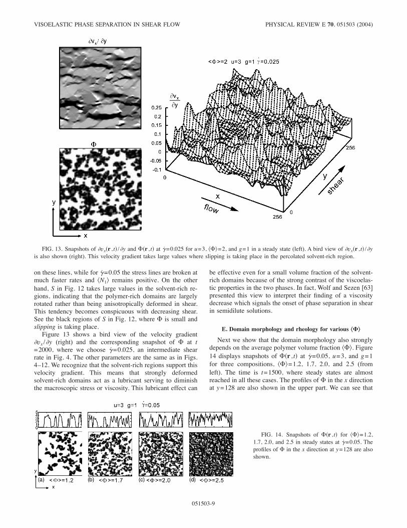
on these lines, while for #̇=0.05 the stress lines are broken atmuch faster rates and $N1% remains positive. On the otherhand, S in Fig. 12 takes large values in the solvent-rich re-gions, indicating that the polymer-rich domains are largelyrotated rather than being anisotropically deformed in shear.This tendency becomes conspicuous with decreasing shear.See the black regions of S in Fig. 12, where , is small andslipping is taking place.Figure 13 shows a bird view of the velocity gradient

!vx /!y (right) and the corresponding snapshot of , at t=2000, where we choose #̇=0.025, an intermediate shearrate in Fig. 4. The other parameters are the same as in Figs.4–12. We recognize that the solvent-rich regions support thisvelocity gradient. This means that strongly deformedsolvent-rich domains act as a lubricant serving to diminishthe macroscopic stress or viscosity. This lubricant effect can

be effective even for a small volume fraction of the solvent-rich domains because of the strong contrast of the viscoelas-tic properties in the two phases. In fact, Wolf and Sezen [63]presented this view to interpret their finding of a viscositydecrease which signals the onset of phase separation in shearin semidilute solutions.

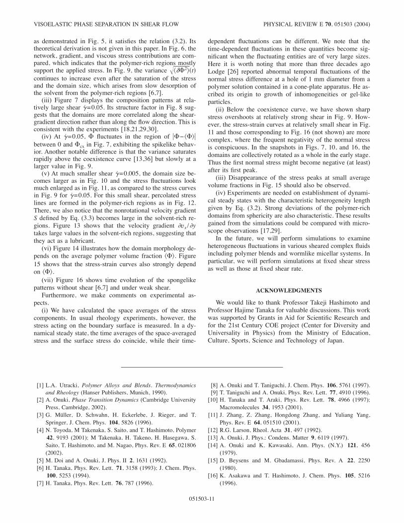
E. Domain morphology and rheology for various !"‹Next we show that the domain morphology also strongly

depends on the average polymer volume fraction $,%. Figure14 displays snapshots of ,!r , t" at #̇=0.05, u=3, and g=1for three compositions, $,%=1.2, 1.7, 2.0, and 2.5 (fromleft). The time is t=1500, where steady states are almostreached in all these cases. The profiles of , in the x directionat y=128 are also shown in the upper part. We can see that

FIG. 13. Snapshots of !vx!r , t" /!y and ,!r , t" at #̇=0.025 for u=3, $,%=2, and g=1 in a steady state (left). A bird view of !vx!r , t" /!yis also shown (right). This velocity gradient takes large values where slipping is taking place in the percolated solvent-rich region.

FIG. 14. Snapshots of ,!r , t" for $,%=1.2,1.7, 2.0, and 2.5 in steady states at #̇=0.05. Theprofiles of , in the x direction at y=128 are alsoshown.

VISOELASTIC PHASE SEPARATION IN SHEAR FLOW PHYSICAL REVIEW E 70, 051503 (2004)

051503-9

,.,cx.3.7 within the polymer-rich regions. With increas-ing $,%, the collision frequency among the domains in-creases and the domain size decreases. In fact, the domainsize RD determined from the perimeter length is 13.75,10.83, and 6.67 for $,%=1.7, 2.0, and 2.5, respectively. Evenfor $,%=1.2, the polymer-rich domain collide frequently andthe domain shapes largely deviate from sphericity. In Fig. 15,we plot time evolutions of the space-averaged shear stress$0xy%!t" for these values of $,%. In the dynamical steadystate, we calculate the normalized shear viscosity increase9) /)0= $0xy% / #̇)0−1. If it is averaged over time, it is givenby 2, 4, 6.5, and 15 for $,%=1.2, 1.7, 2.0, and 2.5, respec-tively. It is remarkable that the stress overshoot is nonexist-ent at small $,% and gradually develops with increasing $,%.

F. Deformation of spongelike domains at small shear

Finally, we examine how the spongelike domain structureobserved by Tanaka and co-workers [6,7] is deformed byshear flow. On the left of Fig. 16 we show one example ofsuch a domain structure without shear for $,%=1.2, u=3,

and g=1, where the polymer-rich regions are percolated de-spite relatively small $,% [9,10]. The right part is the resultunder shear #̇=0.005 with the other parameters being com-mon, where the applied strain #̇t is 1, 2, 5, and 10 at t=200, 400, 1000, and 2000 for the given snapshots, respec-tively. For this weak shear rate, the initial stage of phaseseparation is not much different from the case without shearbut the coarsening is quickened as in Fig. 4 for $,%=2. Herethe polymer-rich domains are gradually thickened but remainhighly extended in the flow direction, while the domains inFig. 14(a) are torn into pieces because of larger shear #̇=0.05. Also in this case the average shear stress $0xy%!t" andnormal stress difference $N1!t"% exhibit chaotic behavior andthe product $0xy%!t"R!t" tends to a constant !#2.4". Again asin Fig. 11, the negativity of the normal stress difference isconspicuous in the early stage (not shown here).

IV. SUMMARY AND CONCLUDING REMARKS

Though performed in two dimensions, we have numeri-cally solved the two-fluid dynamic model of sheared semidi-lute polymer solutions with theta solvent, where the chaindeformations are represented by the conformation tensor Wij.The free-energy density depends on Wij as well as the poly-mer volume fraction ' as in Eq. (2.3). In our simulations, theinitial value of the composition is random as described at thebeginning of Sec. III, but the thermal Langevin noise termsin the dynamic equations are neglected for t:0. The subse-quent heterogeneous fluctuations are produced by the nonlin-ear interactions among the fluctuations and not by the ther-mal noise.We summarize our main results.(i) With varying the parameter g representing the magni-

tude of the shear modes, we have examined spinodal decom-position as in Figs. 2 and 3, which show the crossover of thedomain growth from Newtonian to viscoelastic fluids. Thedomain growth is nearly stopped for g$0.1 at relativelylarge shear within our simulation time.

(ii) The domain growth in spinodal decomposition hasbeen examined at g=1 with varying #̇ in Fig. 4. The domainsize RD in steady states becomes finer with increasing #̇ and,

FIG. 15. Time evolution of $0xy%!t" at various $,%. The corre-sponding composition patters are shown in Fig. 14. The overshootdisappears at small $,%.

FIG. 16. Spongelike domain structures with-out shear (left) and under shear #̇=0.005 (right)for $,%=1.2, u=3, and g=1.

IMAEDA, FURUKAWA, AND ONUKI PHYSICAL REVIEW E 70, 051503 (2004)

051503-10

as demonstrated in Fig. 5, it satisfies the relation (3.2). Itstheoretical derivation is not given in this paper. In Fig. 6, thenetwork, gradient, and viscous stress contributions are com-pared, which indicates that the polymer-rich regions mostlysupport the applied stress. In Fig. 9, the variance 2$&,2%!t"continues to increase even after the saturation of the stressand the domain size, which arises from slow desorption ofthe solvent from the polymer-rich regions [6,7].

(iii) Figure 7 displays the composition patterns at rela-tively large shear #̇=0.05. Its structure factor in Fig. 8 sug-gests that the domains are more correlated along the shear-gradient direction rather than along the flow direction. This isconsistent with the experiments [18,21,29,30].

(iv) At #̇=0.05, , fluctuates in the region of -,− $,%-between 0 and ,cx in Fig. 7, exhibiting the spikelike behav-ior. Another notable difference is that the variance saturatesrapidly above the coexistence curve [13,36] but slowly at alarger value in Fig. 9.

(v) At much smaller shear #̇=0.005, the domain size be-comes larger as in Fig. 10 and the stress fluctuations lookmuch enlarged as in Fig. 11, as compared to the stress curvesin Fig. 9 for #̇=0.05. For this small shear, percolated stresslines are formed in the polymer-rich regions as in Fig. 12.There, we also notice that the nonrotational velocity gradientS defined by Eq. (3.3) becomes large in the solvent-rich re-gions. Figure 13 shows that the velocity gradient !vx /!ytakes large values in the solvent-rich regions, suggesting thatthey act as a lubricant.

(vi) Figure 14 illustrates how the domain morphology de-pends on the average polymer volume fraction $,%. Figure15 shows that the stress-strain curves also strongly dependon $,%.

(vii) Figure 16 shows time evolution of the spongelikepatterns without shear [6,7] and under weak shear.Furthermore, we make comments on experimental as-

pects.(i) We have calculated the space averages of the stress

components. In usual rheology experiments, however, thestress acting on the boundary surface is measured. In a dy-namical steady state, the time averages of the space-averagedstress and the surface stress do coincide, while their time-

dependent fluctuations can be different. We note that thetime-dependent fluctuations in these quantities become sig-nificant when the fluctuating entities are of very large sizes.Here it is worth noting that more than three decades agoLodge [26] reported abnormal temporal fluctuations of thenormal stress difference at a hole of 1 mm diameter from apolymer solution contained in a cone-plate apparatus. He as-cribed its origin to growth of inhomogeneities or gel-likeparticles.

(ii) Below the coexistence curve, we have shown sharpstress overshoots at relatively strong shear in Fig. 9. How-ever, the stress-strain curves at relatively small shear in Fig.11 and those corresponding to Fig. 16 (not shown) are morecomplex, where the frequent negativity of the normal stressis conspicuous. In the snapshots in Figs. 7, 10, and 16, thedomains are collectively rotated as a whole in the early stage.Thus the first normal stress might become negative (at least)after its first peak.

(iii) Disappearance of the stress peaks at small averagevolume fractions in Fig. 15 should also be observed.

(iv) Experiments are needed on establishment of dynami-cal steady states with the characteristic heterogeneity lengthgiven by Eq. (3.2). Strong deviations of the polymer-richdomains from sphericity are also characteristic. These resultsgained from the simulations could be compared with micro-scope observations [17,29].In the future, we will perform simulations to examine

heterogeneous fluctuations in various sheared complex fluidsincluding polymer blends and wormlike micellar systems. Inparticular, we will perform simulations at fixed shear stressas well as those at fixed shear rate.

ACKNOWLEDGMENTS

We would like to thank Professor Takeji Hashimoto andProfessor Hajime Tanaka for valuable discussions. This workwas supported by Grants in Aid for Scientific Research andfor the 21st Century COE project (Center for Diversity andUniversality in Physics) from the Ministry of Education,Culture, Sports, Science and Technology of Japan.

[1] L.A. Utracki, Polymer Alloys and Blends. Thermodynamicsand Rheology (Hanser Publishers, Munich, 1990).

[2] A. Onuki, Phase Transition Dynamics (Cambridge UniversityPress, Cambridge, 2002).

[3] G. Müller, D. Schwahn, H. Eckerlebe, J. Rieger, and T.Springer, J. Chem. Phys. 104, 5826 (1996).

[4] N. Toyoda, M Takenaka, S. Saito, and T. Hashimoto, Polymer42, 9193 (2001); M Takenaka, H. Takeno, H. Hasegawa, S.Saito, T. Hashimoto, and M. Nagao, Phys. Rev. E 65, 021806(2002).

[5] M. Doi and A. Onuki, J. Phys. II 2, 1631 (1992).[6] H. Tanaka, Phys. Rev. Lett. 71, 3158 (1993); J. Chem. Phys.

100, 5253 (1994).[7] H. Tanaka, Phys. Rev. Lett. 76, 787 (1996).

[8] A. Onuki and T. Taniguchi, J. Chem. Phys. 106, 5761 (1997).[9] T. Taniguchi and A. Onuki, Phys. Rev. Lett. 77, 4910 (1996).

[10] H. Tanaka and T. Araki, Phys. Rev. Lett. 78, 4966 (1997);Macromolecules 34, 1953 (2001).

[11] J. Zhang, Z. Zhang, Hongdong Zhang, and Yuliang Yang,Phys. Rev. E 64, 051510 (2001).

[12] R.G. Larson, Rheol. Acta 31, 497 (1992).[13] A. Onuki, J. Phys.: Condens. Matter 9, 6119 (1997).[14] A. Onuki and K. Kawasaki, Ann. Phys. (N.Y.) 121, 456

(1979).[15] D. Beysens and M. Gbadamassi, Phys. Rev. A 22, 2250

(1980).[16] K. Asakawa and T. Hashimoto, J. Chem. Phys. 105, 5216

(1996).

VISOELASTIC PHASE SEPARATION IN SHEAR FLOW PHYSICAL REVIEW E 70, 051503 (2004)

051503-11

[17] T. Hashimoto, K. Matsuzaka, E. Moses, and A. Onuki, Phys.Rev. Lett. 74, 126 (1995).

[18] X.L. Wu, D.J. Pine, and P.K. Dixon, Phys. Rev. Lett. 68, 2408(1991).

[19] T. Hashimoto and K. Fujioka, J. Phys. Soc. Jpn. 60, 356(1991); T. Hashimoto and T. Kume, ibid. 61, 1839 (1992); H.Murase, T. Kume, T. Hashimoto, Y. Ohta, and T. Mizukami,Macromolecules 28, 7724 (1995).

[20] T. Kume, T. Hattori, and T. Hashimoto, Macromolecules 30,427 (1997).

[21] S. Saito and T. Hashimoto, J. Chem. Phys. 114, 10531 (2001);S. Saito, T. Hashimoto, I. Morfin, P. Linder, and F. Boue, ibid.35, 445 (2002).

[22] J. van Egmond, D.E. Werner, and G.G. Fuller, J. Chem. Phys.96, 7742 (1992); J. van Egmond and G. Fuller, Macromol-ecules 26, 7182 (1993).

[23] A.I. Nakatani, J.F. Douglas, Y.-B. Ban, and C.C. Han, J. Chem.Phys. 100, 3224 (1994).

[24] I. Morfin, P. Linder, and F. Boue, Macromolecules 32, 7208(1999).

[25] K. Migler, C. Liu, and D.J. Pine, Macromolecules 29, 1422(1996).

[26] A.S. Lodge, Polymer 2, 195 (1961).[27] A. Peterlin and D.T. Turner, J. Polym. Sci., Part B: Polym.

Lett. 3, 517 (1965).[28] J.J. Magda, C.-S. Lee, S.J. Muller, and R.G. Larson, Macro-

molecules 26, 1696 (1993).[29] E. Moses, T. Kume, and T. Hashimoto, Phys. Rev. Lett. 72,

2037 (1994).[30] E.K. Hobbie, H.S. Jeon, H. Wang, H. Kim, D.J. Stout, and

C.C. Han, J. Chem. Phys. 117, 6350 (2002).[31] E. Helfand and G.H. Fredrickson, Phys. Rev. Lett. 62, 2468

(1989).[32] A. Onuki, Phys. Rev. Lett. 62, 2472 (1989); A. Onuki, J. Phys.

Soc. Jpn. 59, 3423 (1990); 59, 3427 (1990).[33] S.T. Milner, Phys. Rev. Lett. 66, 1477 (1991); Phys. Rev. E

48, 3674 (1993).[34] H. Ji and E. Helfand, Macromolecules 28, 3869 (1995).[35] G. H. Fredrickson, J. Chem. Phys. 117, 6810 (2002).[36] A. Onuki, R. Yamamoto, and T. Taniguchi, J. Phys. II 7, 295

(1997); Prog. Colloid Polym. Sci. 106, 150 (1997).[37] T. Okuzono, Mod. Phys. Lett. A 11, 379 (1997).[38] X.-F. Yuan and L. Jupp, Europhys. Lett. 60, 691 (2002).[39] L. Jupp, T. Kawakatsu, and X.-F. Yuan, J. Chem. Phys. 119,

6361 (2003).[40] S. M. Fielding and P. D. Olmsted, Phys. Rev. E 68, 036313

(2003).[41] B. Chakrabarti, M. Das, C. Dasgupta, S. Ramaswamy, and

A.K. Sood, Phys. Rev. Lett. 92, 055501 (2004).[42] F. Pignon, A. Magnin, and J.-M. Piau, J. Rheol. 40, 573

(1996); R. Bandyopadhyay and A. K. Sood, Europhys. Lett.56, 447 (2001); J.-B. Salmon, S. Manneville, and A. Colin,

Phys. Rev. E 68, 051504 (2003).[43] M.E. Cates, D.A. Head, and A. Ajdari, Phys. Rev. E 66,

025202 (2002); G. Picard, A. Ajdari, L. Bocquet, and F. Le-queux, ibid. 66, 051501 (2002).

[44] X.-F. Yuan, Europhys. Lett. 46, 542 (1999); P. D. Olmsted, O.Radulescu, and C.-Y.D. Lu, J. Rheol. 44, 257 (2000).

[45] P.G. de Gennes, Scaling Concepts in Polymer Physics (CornellUniversity Press, Ithaca 1980).

[46] T. Ohta, H. Nozaki, and M. Doi, J. Chem. Phys. 93, 2664(1990); D.H. Rothman, Europhys. Lett. 14, 337 (1991); P. Pa-dilla and S. Toxvaerd, J. Chem. Phys. 106, 2342 (1997); A. J.Wagner and J. M. Yeomans, Phys. Rev. E 59, 4366 (1999).

[47] L. Berthier, Phys. Rev. E 63, 051503 (2001).[48] A. Frischknecht, Phys. Rev. E 56, 6970 (1997); 58, 3495

(1998).[49] K.B. Migler, Phys. Rev. Lett. 86, 1023 (2001).[50] M. Grmela, Phys. Lett. A 130, 81 (1988); H. C. Öttinger and

M. Grmela, Phys. Rev. E 56, 6633 (1997).[51] A.N. Beris and B.J. Edwards, Thermodynamics of Flowing

Systems (Oxford University Press, Oxford, 1994).[52] M. Adam and M. Delsanti, J. Phys. (Paris) 44, 1185 (1983);

45, 1513 (1984).[53] Y. Takahashi, Y. Isono, I. Noda, and M. Nagasawa, Macromol-

ecules 18, 1002 (1985).[54] R.G. Larson, The Structure and Rheology of Complex Fluids

(Oxford University Press, Oxford, 1999).[55] The factor 1 / !1+Q" in Eq. (2.21) serves to stabilize numerical

integration of Eq. (2.11).[56] J.L. White and A.B. Metzner, J. Appl. Polym. Sci. 8, 1367

(1963).[57] A. Onuki, Phys. Rev. A 35, 5149 (1987).[58] We have also performed simulations with the mesh size taken

to be 9x=! /22 and ! /2. Then the curves in the bottom platein Fig. 7 coincide within 5% without any qualitative differ-ences. The behavior of , in the spikelike regions in Fig. 7 arewell described even with 9x=!.

[59] A. Onuki, J. Phys. Soc. Jpn. 66, 1836 (1997).[60] At t=0, we consider the variance of the deviation 3dr&' /'c!d

averaged in one unit cell. Its thermal value is of order ,−1/2 inthe semidilute theta condition.

[61] T. Baumberger, F. Perrot, and D. Beysens, Phys. Rev. A 46,7636 (1992).

[62] A. Onuki, Europhys. Lett. 28, 175 (1994). In the Newtoniancase, the ratio CNew/# is of order ' if the droplet volumefraction is considerably smaller than 1/2 and if the viscosityratio )1 /)2 is close to 1. If )1 /)2 much deviates from 1, CNewis a complicated function of ' and )1 /)2. For '#1/2, thedomains can be extended into very long cylinders resulting ina string phase [17,48,49].

[63] B.A. Wolf and M.C. Sezen, Macromolecules 10, 1010 (1977);B.A. Wolf and R. Jend, ibid. 12, 732 (1979).

IMAEDA, FURUKAWA, AND ONUKI PHYSICAL REVIEW E 70, 051503 (2004)

051503-12