THE 19TH INTERNATIONAL CONFERENCE ON COMPOSITE MATERIALS

Abstract Among the passive control techniques for vibration attenuation in composite structures demonstrated in the last decades, the use of viscoelastic material as a damping core in laminated beam like components is an interesting possibility but has not yet received sufficient attention so far. In order to gain an insight into this interest and develop more accurate and efficient viscoelastic-based vibration control methods, this paper presents a finite element method (FEM) for damping modeling of a multilayer composite structure, with a viscoelastic core sandwiched between elastic layers including piezoelectric layers. Emphasis is put not only on the numerical modeling integrating FEM with the Golla-Hughes-McTavish (GHM) and the Anelastic Displacement Fields (ADF) method method, which is used to illustrate the effects of viscoelastic layer and the vascular cooling channels, but also on practical engineering aspects related with the use of modal testing for the experimental assessment of efficiency of damping treatments. In particular, different configurations of damping treatments, spatial FE modeling, mathematical descriptions of viscoelastic frequency-dependent material damping and their implementation into FE frameworks and the use of different solution methods are discussed.

1 Introduction

As a potential solution to lightweight skins for spacecraft, a functional graded composite beam studied in this paper is required to be able to operate in extreme conditions. Figure 1 illustrates the configuration of the layered composite beam under consideration. There are five component layers: a

oxide ceramic outer layer capable of withstanding high temperatures up to 1300°C, a functionally graded ceramic layer combining shape memory alloy (SMA) properties of NiTi together with the MAX phase layer Ti2AlC (called Graded Ceramic/Metal Composite, or GCMeC), a high temperature sensor patch, followed by a polymer matrix composite (PMC) laced with vascular cooling channels all held together with various epoxies, and then a layer of a piezoelectric actuator. The key effect not well modeled in this structure is its damping property. Due to the recoverable nature of SMA and adhesive property of Ti2AlC, the damping behavior of the GCMeC is largely frequency-dependent viscoelastic.

Figure 1 The example of a functional graded composite beam. Even the viscoelastic materials have wide application in solving damping problems of many engineering systems [1-4], such as aircraft, space structures, automobiles, buildings, bridges and so on, their damping models in most available commercial finite element software do not explicitly represent the environmental effected behaviors of actual materials (such as excitation frequency, ambient temperature, dynamic loads, etc.). One of the effective viscoelastic damping models in engineering application was developed by Golla and Hughes [5] and McTavish and Hughes [6], known as

VISCOELASTIC BEHAVIOR OF A COMPOSITE BEAM USING FINITE ELEMENT METHOD: EXPERIMENTAL AND

NUMERICAL ASSESSMENT

Y. Wang1*, D., Inman1 1 Department of Aerospace Engineering, University of Michigan, Ann Arbor, MI, U.S.A.

*Corresponding author (ywangs@umich.edu)

Keywords: Viscoelastic, Finite Element Method, Golla-Hughes-McTavish (GHM) method, Anelastic Displacement Fields (ADF) method

the Golla-Hughes-McTavish (GHM) method. The GHM method introduces additional coordinates of internal variables using an analogy with a generalized lumped-parameter Maxwell model. The material modulus in Laplace domain is interpreted as a series of mini-oscillators terms [7, 8]. In addition, Lesieutre and Lee [9] introduced the Anelastic Displacement Fields (ADF) method by adding nodal anelastic degrees of freedom to the element nodes and formulating internal strains from internal displacement fields. Both GHM and ADF methods are studied and compared in this paper to account for damping effects over a range of frequencies and complex mode behavior. However, such a multilayer composite structure with a high temperature viscoelastic material based on the concept in Figure 1 is still under construction and has not yet been finished. As an alternative construction technique, an experimental composite structure with viscoelastic damping layer will be fabricated using an ObJet 3D printer, the combination of rapid prototyping and layered composite construction. This technique allows the construction of a functionally graded layered composite without having to glue layers together. This is important because the epoxy normally used to combine the layers introduces unknown amounts of damping due to uncontrollable thickness etc. The uniqueness of this printer is to intersperse droplets of a white ABS plastic material (VeroWhitePlusTM) with a transparent elastomeric material (TangoPlusTM) using a servo-actuated printer head to produce materials of tailorable stiffness and hardness. Table 1 lists material properties of VeroWhiteplus and two other rigid material examples Digital Material (DM) 8425, and DM 8430 to represent the oxide ceramics, the piezoelectric sensor and the piezoelectric actuator, respectively. They are the mixture of the primary material VeroWhitePlus and the secondary material TangoPlus.

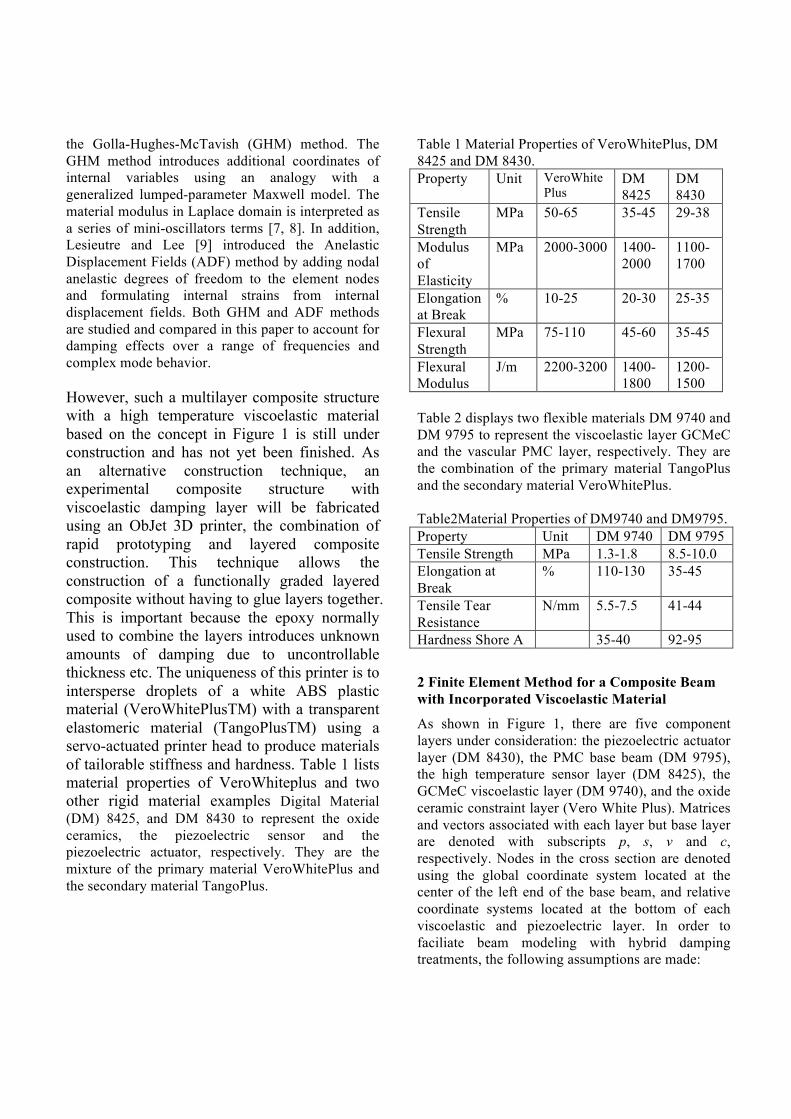
Table 1 Material Properties of VeroWhitePlus, DM 8425 and DM 8430. Property Unit VeroWhite

Plus DM 8425

DM 8430

Tensile Strength

MPa 50-65 35-45 29-38

Modulus of Elasticity

MPa 2000-3000 1400-2000

1100-1700

Elongation at Break

% 10-25 20-30 25-35

Flexural Strength

MPa 75-110 45-60 35-45

Flexural Modulus

J/m 2200-3200 1400-1800

1200-1500

Table 2 displays two flexible materials DM 9740 and DM 9795 to represent the viscoelastic layer GCMeC and the vascular PMC layer, respectively. They are the combination of the primary material TangoPlus and the secondary material VeroWhitePlus. Table2Material Properties of DM9740 and DM9795. Property Unit DM 9740 DM 9795 Tensile Strength MPa 1.3-1.8 8.5-10.0 Elongation at Break

% 110-130 35-45

Tensile Tear Resistance

N/mm 5.5-7.5 41-44

Hardness Shore A 35-40 92-95

2 Finite Element Method for a Composite Beam with Incorporated Viscoelastic Material

As shown in Figure 1, there are five component layers under consideration: the piezoelectric actuator layer (DM 8430), the PMC base beam (DM 9795), the high temperature sensor layer (DM 8425), the GCMeC viscoelastic layer (DM 9740), and the oxide ceramic constraint layer (Vero White Plus). Matrices and vectors associated with each layer but base layer are denoted with subscripts p, s, v and c, respectively. Nodes in the cross section are denoted using the global coordinate system located at the center of the left end of the base beam, and relative coordinate systems located at the bottom of each viscoelastic and piezoelectric layer. In order to faciliate beam modeling with hybrid damping treatments, the following assumptions are made:

3

VISCOELASTIC BEHAVIOR OF A COMPOSITE BEAM USING FINITE ELEMENT METHOD: EXPERIMENTAL AND NUMERICAL ASSESSMENT

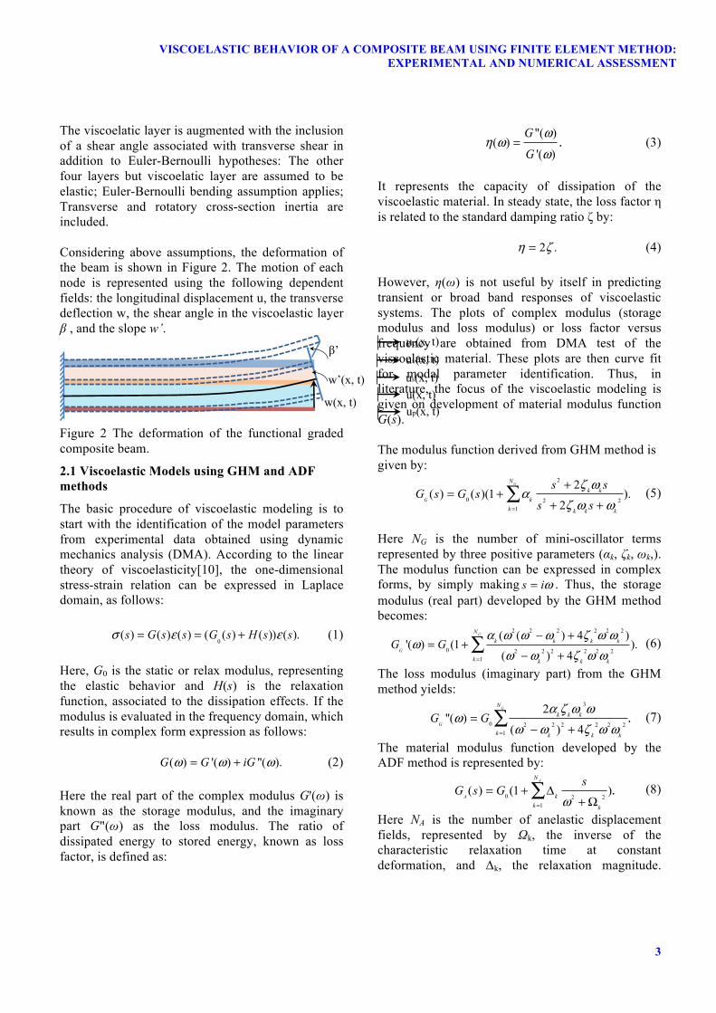
The viscoelatic layer is augmented with the inclusion of a shear angle associated with transverse shear in addition to Euler-Bernoulli hypotheses: The other four layers but viscoelatic layer are assumed to be elastic; Euler-Bernoulli bending assumption applies; Transverse and rotatory cross-section inertia are included. Considering above assumptions, the deformation of the beam is shown in Figure 2. The motion of each node is represented using the following dependent fields: the longitudinal displacement u, the transverse deflection w, the shear angle in the viscoelastic layer β , and the slope w’.

w(x, t)

w’(x, t)

β’

u(x, t)us(x, t)uv(x, t)

up(x, t)

uc(x, t)

Figure 2 The deformation of the functional graded composite beam.

2.1 Viscoelastic Models using GHM and ADF methods

The basic procedure of viscoelastic modeling is to start with the identification of the model parameters from experimental data obtained using dynamic mechanics analysis (DMA). According to the linear theory of viscoelasticity[10], the one-dimensional stress-strain relation can be expressed in Laplace domain, as follows:

σ (s) = G(s)ε (s) = (G0(s) + H (s))ε (s). (1)

Here, G0 is the static or relax modulus, representing the elastic behavior and H(s) is the relaxation function, associated to the dissipation effects. If the modulus is evaluated in the frequency domain, which results in complex form expression as follows:

( ) '( ) ''( ).G G iGω ω ω= + (2)

Here the real part of the complex modulus G'(ω) is known as the storage modulus, and the imaginary part G"(ω) as the loss modulus. The ratio of dissipated energy to stored energy, known as loss factor, is defined as:

"( )( )

'( ).G

G

ωη ω

ω= (3)

It represents the capacity of dissipation of the viscoelastic material. In steady state, the loss factor η is related to the standard damping ratio ζ by:

2 .η ζ= (4) However, η(ω) is not useful by itself in predicting transient or broad band responses of viscoelastic systems. The plots of complex modulus (storage modulus and loss modulus) or loss factor versus frequency are obtained from DMA test of the viscoelastic material. These plots are then curve fit for modal parameter identification. Thus, in literature, the focus of the viscoelastic modeling is given on development of material modulus function G(s). The modulus function derived from GHM method is given by:

2

0 2 21

2( ) ( )(1 ).

2

G

G

Nk k

kk k k k

s sG s G s

s s

ζ ωα

ζ ω ω=

+= +

+ +∑ (5)

Here NG is the number of mini-oscillator terms represented by three positive parameters (αk, ζk, ωk,). The modulus function can be expressed in complex forms, by simply making s iω= . Thus, the storage modulus (real part) developed by the GHM method becomes:

2 2 2 2 2 2

0 2 2 2 2 2 21

( ( ) 4 )'( ) (1 ).

( ) 4

G

G

Nk k k k

k k k k

G Gα ω ω ω ζ ω ω

ωω ω ζ ω ω=

− += +

− +∑ (6)

The loss modulus (imaginary part) from the GHM method yields:

3

0 2 2 2 2 2 21

2''( )

( ) 4.

G

G

Nk k k

k k k k

G Gα ζ ω ω

ωω ω ζ ω ω=

=− +

∑ (7)

The material modulus function developed by the ADF method is represented by:

0 2 2

1

( ) (1 ).A

A

N

kk k

sG s G

ω=

= + Δ+Ω

∑ (8)

Here NA is the number of anelastic displacement fields, represented by Ωk, the inverse of the characteristic relaxation time at constant deformation, and Δk, the relaxation magnitude.

Decompose the modulus function in complex form, leads to the expression of the storage modulus by the ADF method:

2

0 21

( / )'( ) (1 )

( / ).

1A

A

Nk

kk k

G Gω

ωω=

Ω= + Δ

+ Ω∑ (9)

The loss modulus from the ADF method becomes:

2

1

/''( )

( / ).

1A

A

Nk

r kk k

G Gω

ωω=

Ω= Δ

+ Ω∑ (10)

Therefore, the determination of material parameters are carried out by formulating an optimization problem in which the objective function represents the difference between the experimental data points and the corresponding model predictions. The numbers of design variables, for the GHM and ADF method are 1+3NG and 1+2NA, respectively.

2.2 Viscoelastic Models using GHM and ADF methods

As mentioned earlier, the viscoelastic behavior is decomposed by an elastic part and an anelastic part. Thus, the finite element equation of motion for the viscoelastic structure may be expressed in the following standard second order form:

Mq + D q + (K e +K v (s))q = F (11)

Here N N×∈M ° is the symmetric and positive definite mass matrix, N N×∈D ° is the symmetric and semi-positive definite viscous damping matrix, and , N N

e v

×∈K K ° is the elastic and viscoelastic stiffness matrix (symmetric and semi-positive definite). Here , N∈q F ° represents the displacement and loading

factor, respectively. As stated earlier, the viscoelastic stiffness matrix can be factored out of the stiffness matrix and made dependent on the frequency according to the particular viscoelastic model as

( ) .v vG s=K K The definition and derivation of each matrix and vector is not provided here. The interested reader is referred to the reference [9,10] for the details. The derivation of temperature-dependent viscoelastic modeling is not provided here either. The interested read is referred to reference [11] for the details. Substituting the GHM model Equation (5) into Equation (31), one obtains:

2

2

0 21

2( (1 )) ( ) ( )

2

GNk k

e v kk k k k

s ss s G s s

s s

ζ ωα

ζ ω ω=

++ + + + =

+ +∑M D K K q F (12)

The principle of GHM method is to produce a second degree of freedom, by introducing an auxiliary coordinate zk, which is defined according to:

z

k(s) =

ωk

2

s2 + 2ζkω

ks +ω

k

2q(s) (13)

The model represented by Equation (32) can be recovered once this auxiliary DOF is eliminated. Substituting Equation (33) into Equation (32), one obtains the following equation of motion:

MGqG+ D

GqG+K

GqG= F (14)

Here each matrix and vector is defined as follows:

0

2

0

2

1

1G

G

k v

k

N v

k

αω

αω

=

⎛ ⎞⎜ ⎟⎜ ⎟⎜ ⎟⎜ ⎟⎜ ⎟⎜ ⎟⎜ ⎟⎝ ⎠

M 0 0

0 K 0

M0 0

0 0 K

L

M

M O

L

,

0

2

0

2

2

2G

G

kk v

k

kN v

k

ζα

ω

ζα

ω

=

⎛ ⎞⎜ ⎟⎜ ⎟⎜ ⎟⎜ ⎟⎜ ⎟⎜ ⎟⎜ ⎟⎝ ⎠

D 0 0

0 K 0

D0 0

0 0 K

L

M

M O

L

,

0 0

0 0

2

0 0

1( )

( )

G

G G

G

e v i v N v

T

i v k v

k

T

N v N v

α α

α αω

α α

∞+ − −

−=

−

⎛ ⎞⎜ ⎟⎜ ⎟⎜ ⎟⎜ ⎟⎜ ⎟⎜ ⎟⎝ ⎠

K K K K

K K 0K

0 0

K 0 K

L

M

M O

L

,

1{ , , , }

{ ,0, , 0}

G NG

T

T

z z=

=

q q

F F

L

L.

5

VISCOELASTIC BEHAVIOR OF A COMPOSITE BEAM USING FINITE ELEMENT METHOD: EXPERIMENTAL AND NUMERICAL ASSESSMENT

Here , , G G

G G G

t t×∈M D K ° with (1 )G G

N Nt = + . 0

0v vG=K K is the static stiffness matrix and 0 (1 )kv v kα∞ = +∑K K is the dynamic stiffness matrix.

Considering the ADF method, the equation of motion can be obtained by substituting Equation (8) into Equation (31) as follows:

(s2M + sD + K

e+ G

0K

v(1+ Δ

k

s

ω 2 +Ωk

2)

k=1

NA

∑ )q(s) = F(s) (15)

The principle of the ADF method is to assume that the total deformation of the viscoelastic layer (shear angle β ) is the sum of an elastic part Eβ , where the strain is proportional to the stress and an anelastic part Aβ , which captures its relaxation behavior, that

is β = β E + β A . Introducing the anelastic part, results the following equation of motion:

M AqA + DA

qA +K AqA = F (16) Here each matrix and vector is defined as follows:

A=

⎛ ⎞⎜ ⎟⎜ ⎟⎜ ⎟⎜ ⎟⎝ ⎠

M 0 0

0 0 0M

0 0

0 0 0

L

M

M O

L

,

1

1

A

A

v

N

v

n

C

C

∞

∞

Ω=

Ω

⎛ ⎞⎜ ⎟⎜ ⎟⎜ ⎟⎜ ⎟⎜ ⎟⎜ ⎟⎜ ⎟⎝ ⎠

D 0 0

0 K 0

D0 0

0 0 K

L

M

M O

L

,

( )

( )A

A

e v v v

T

v k v

T

v N v

C

C

∞ ∞ ∞

∞ ∞

∞ ∞

+ − −

−=

−

⎛ ⎞⎜ ⎟⎜ ⎟⎜ ⎟⎜ ⎟⎝ ⎠

K K K K

K K 0K

0 0

K 0 K

L

M

M O

L

,

1{ , , , } , { ,0, ,0}A A

a a T T

Nq q= =q q F FL L .

Here, , , A A

A A A

t t×∈M D K °

with (1 )A AN Nt = + and

0 (1 )kv v kG∞ = + Δ∑K K ,

1 AN

kkk

k

C+ Δ

=Δ∑ .

3 Numerical Simulation and Experimental Validation

The GHM and ADF models addressed in this paper are evaluated on the cantilever beam shown in Figure 1, the proposed functionally graded composite beam, consisting five layers of the Oxide Ceramic, PZT sensor, PMC base beam, the viscoelastic layer, and the piezoelectric constraint layer, but represented by a 3D printed prototype consisting five layers of VeroWhitePlus, DM9740, DM8425, DM9795, and DM8430, respectively. Table 3 lists the mechanical and material properties of the proposed functionally graded composite beam. The density and elastic modulus of the piezoelectric actuator (Micro-Fiber Composite) is experimentally obtained from the authors' early work [11]. The mechanical and material properties of PMC (carbon fiber and epoxy), GCMeC (Ti2AlC and NiTi) and Oxide ceramic (Al2O3 and TiO2) are estimated from pervious references [12, 13]. Note that, the length here is free length, not including the clamped length of 38 mm. Table 3 Mechanical and Material Properties of Each Layer Component Used in Numerical Examples. Dimension

(mm*mm*mm) Density (kg/m3)

Elastic Modulus (GPa)

PZT Actuator

300 * 30 * 0.3 5440 33

PMC 338 * 30 * 0.6 1911 10 PZT Sensor

300 * 30 * 0.03 5440 720

GCMeC 300 *30 *0.3 4110 G(ω) Oxide Ceramic

300 * 30 * 0.018

3600 205

Table 4 lists the mechanical and material properties of the 3D printed composite beam. It is interesting to find that the measurement of the elastic modulus of each material yields big difference using static and dynamic ways, as listed in Table 4. The static measurement was carried on using MTS machine,

following the ASTM D 638, standard test methods for tensile properties of plastics. The elastic modulus was also calculated by measuring the dynamic response of the cantilever beam. One can find that the higher percentage of TangoPlus, the more flexible the composite material, and the bigger difference of static and dynamic modulus measurements. Experiments show that the dynamic measurement gives more accurate results. Details are given in the end of this paper, as seen in Figure 8 and Figure 9. Table 4 Mechanical and Material Properties of the 3D printed Composite Beam used in Numerical Examples.

Material Dimension (mm*mm *mm)

Density (kg/m3)

Elastic Modulus (Static) (GPa)

Elastic Modulus (Dynamic) (GPa)

Error

DM8430 338*30*0.63

1180 1.56 1.97 21%

DM9795 338*30*1.8

1135 0.16 0.55 71%

DM8425 338*30*0.12

1174 1.90 2.47 23%

DM9740 338*30*2.1

1101 G(ω) G(ω) N/A

VeroWhitePlus

338*30*0.12

1178 2.09 2.49 16%

3.1 Parameter Identification using Curve Fitting

As seen from Equations (34) and (35), the inclusion of the dissipative variables in the GHM and ADF models to account for the viscoelastic behavior leads to augmented coupled systems of equations of motion in which the total number of DOF largely exceeds the number of structural DOF. Moreover, for both models, non-positive-definite inertia matrices are obtained. As result, numerical preprocessing is found to be necessary prior to the resolution of the equations for response analyses.

A positive-definite inertia matrix can be obtained for the GHM model by performing the spectral decomposition of the stiffness matrix related to the viscoelastic substructure [6]. The null eigenvalues and corresponding eigenvectors are eliminated and, as result, fewer dissipative coordinates and a positive-definite viscoelastic matrix are obtained. As for the ADF model, it is not possible to obtain a positive-definite mass matrix by using the same approach. However, the problems entailed by the

singularity can be avoided by performing an adequate transformation of augmented system of second-order equations into a state-space first-order form, the dimension of which is, in general, much smaller than that obtained for the GHM model [14].

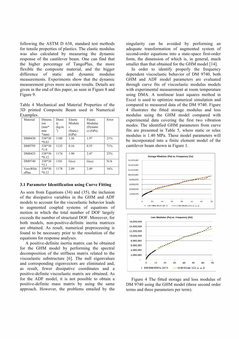
In order to identify properly the frequency dependent viscoelastic behavior of DM 9740, both GHM and ADF model parameters are evaluated through curve fits of viscoelastic modulus models with experimental measurement at room temperature using DMA. A nonlinear least squares method in Excel is used to optimize numerical simulation and compared to measured data of the DM 9740. Figure 4 illustrates the fitted storage modulus and loss modulus using the GHM model compared with experimental data covering the first two vibration modes. The identified GHM parameters from curve fits are presented in Table 5, where static or relax modulus is 1.40 MPa. These model parameters will be incorporated into a finite element model of the cantilever beam shown in Figure 1.

Figure 4 The fitted storage and loss modulus of

DM 9740 using the GHM model (three second order terms and three parameters per term).

7

VISCOELASTIC BEHAVIOR OF A COMPOSITE BEAM USING FINITE ELEMENT METHOD: EXPERIMENTAL AND NUMERICAL ASSESSMENT

Table 5 Identified parameters for the optimized curve fit for DM 9740 using the GHM model (three second order terms and three parameters per term).

k 1 2 3 ωk (rad/s) 50047.905 2111.210 30016.011

ζk 56.076 21.312 0.162 αk 7.954 2.090 1067.507

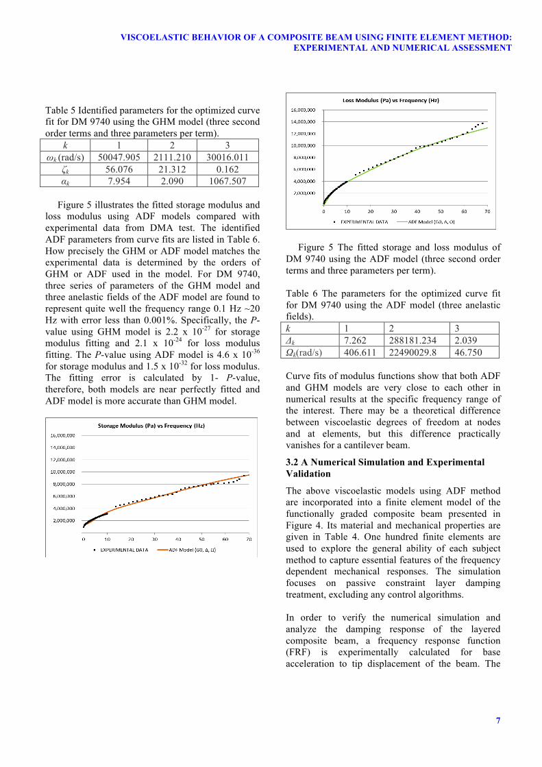
Figure 5 illustrates the fitted storage modulus and

loss modulus using ADF models compared with experimental data from DMA test. The identified ADF parameters from curve fits are listed in Table 6. How precisely the GHM or ADF model matches the experimental data is determined by the orders of GHM or ADF used in the model. For DM 9740, three series of parameters of the GHM model and three anelastic fields of the ADF model are found to represent quite well the frequency range 0.1 Hz ~20 Hz with error less than 0.001%. Specifically, the P-value using GHM model is 2.2 x 10-27 for storage modulus fitting and 2.1 x 10-24 for loss modulus fitting. The P-value using ADF model is 4.6 x 10-36

for storage modulus and 1.5 x 10-32 for loss modulus. The fitting error is calculated by 1- P-value, therefore, both models are near perfectly fitted and ADF model is more accurate than GHM model.

Figure 5 The fitted storage and loss modulus of

DM 9740 using the ADF model (three second order terms and three parameters per term).

Table 6 The parameters for the optimized curve fit for DM 9740 using the ADF model (three anelastic fields). k 1 2 3 Δk 7.262 288181.234 2.039 Ωk(rad/s) 406.611 22490029.8 46.750

Curve fits of modulus functions show that both ADF and GHM models are very close to each other in numerical results at the specific frequency range of the interest. There may be a theoretical difference between viscoelastic degrees of freedom at nodes and at elements, but this difference practically vanishes for a cantilever beam.

3.2 A Numerical Simulation and Experimental Validation

The above viscoelastic models using ADF method are incorporated into a finite element model of the functionally graded composite beam presented in Figure 4. Its material and mechanical properties are given in Table 4. One hundred finite elements are used to explore the general ability of each subject method to capture essential features of the frequency dependent mechanical responses. The simulation focuses on passive constraint layer damping treatment, excluding any control algorithms. In order to verify the numerical simulation and analyze the damping response of the layered composite beam, a frequency response function (FRF) is experimentally calculated for base acceleration to tip displacement of the beam. The

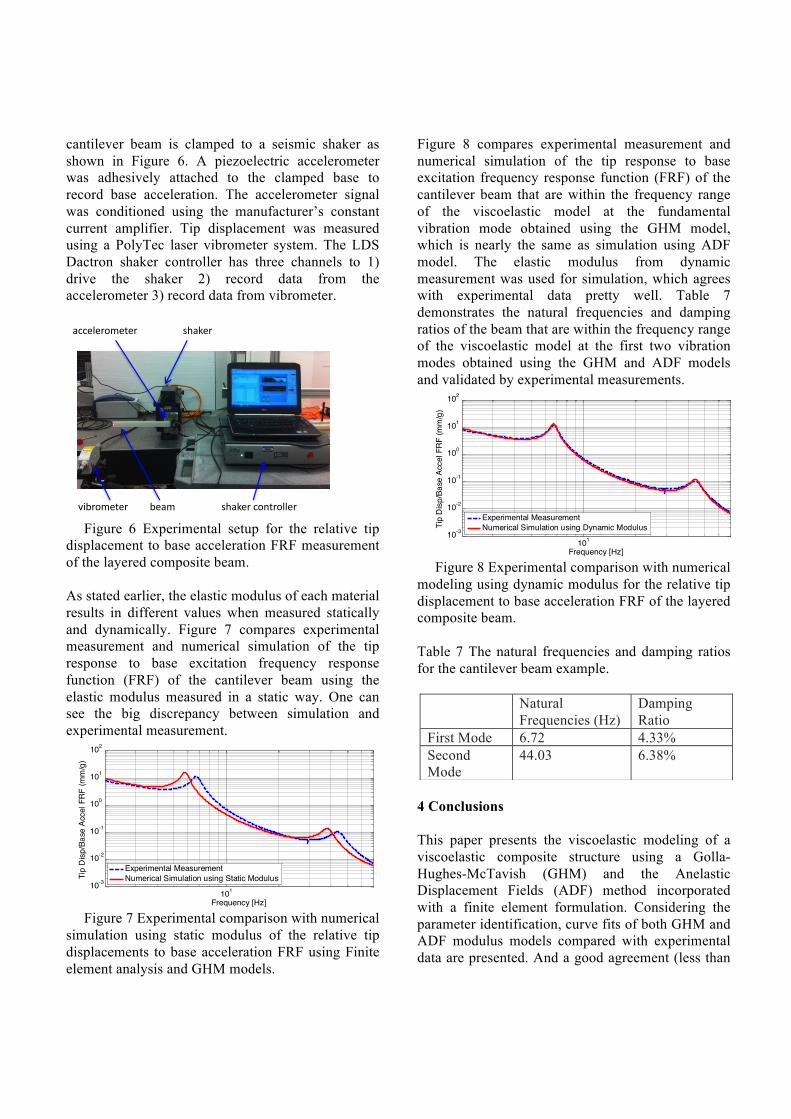
cantilever beam is clamped to a seismic shaker as shown in Figure 6. A piezoelectric accelerometer was adhesively attached to the clamped base to record base acceleration. The accelerometer signal was conditioned using the manufacturer’s constant current amplifier. Tip displacement was measured using a PolyTec laser vibrometer system. The LDS Dactron shaker controller has three channels to 1) drive the shaker 2) record data from the accelerometer 3) record data from vibrometer.

shaker

shaker  controllerbeam

accelerometer

vibrometer

Figure 6 Experimental setup for the relative tip displacement to base acceleration FRF measurement of the layered composite beam. As stated earlier, the elastic modulus of each material results in different values when measured statically and dynamically. Figure 7 compares experimental measurement and numerical simulation of the tip response to base excitation frequency response function (FRF) of the cantilever beam using the elastic modulus measured in a static way. One can see the big discrepancy between simulation and experimental measurement.

10110-3

10-2

10-1

100

101

102

Frequency [Hz]

Tip

Dis

p/Ba

se A

ccel

FR

F (m

m/g

)

Experimental MeasurementNumerical Simulation using Static Modulus

Figure 7 Experimental comparison with numerical

simulation using static modulus of the relative tip displacements to base acceleration FRF using Finite element analysis and GHM models.

Figure 8 compares experimental measurement and numerical simulation of the tip response to base excitation frequency response function (FRF) of the cantilever beam that are within the frequency range of the viscoelastic model at the fundamental vibration mode obtained using the GHM model, which is nearly the same as simulation using ADF model. The elastic modulus from dynamic measurement was used for simulation, which agrees with experimental data pretty well. Table 7 demonstrates the natural frequencies and damping ratios of the beam that are within the frequency range of the viscoelastic model at the first two vibration modes obtained using the GHM and ADF models and validated by experimental measurements.

10110-3

10-2

10-1

100

101

102

Frequency [Hz]

Tip

Dis

p/Ba

se A

ccel

FR

F (m

m/g

)

Experimental MeasurementNumerical Simulation using Dynamic Modulus

Figure 8 Experimental comparison with numerical

modeling using dynamic modulus for the relative tip displacement to base acceleration FRF of the layered composite beam. Table 7 The natural frequencies and damping ratios for the cantilever beam example.

4 Conclusions This paper presents the viscoelastic modeling of a viscoelastic composite structure using a Golla-Hughes-McTavish (GHM) and the Anelastic Displacement Fields (ADF) method incorporated with a finite element formulation. Considering the parameter identification, curve fits of both GHM and ADF modulus models compared with experimental data are presented. And a good agreement (less than

Natural Frequencies (Hz)

Damping Ratio

First Mode 6.72 4.33% Second Mode

44.03 6.38%

9

VISCOELASTIC BEHAVIOR OF A COMPOSITE BEAM USING FINITE ELEMENT METHOD: EXPERIMENTAL AND NUMERICAL ASSESSMENT

0.001% error) is reached. Continuing efforts are addressing the material modulus comparison of the GHM and the ADF model. There may be a theoretical difference between viscoelastic degrees of freedom at nodes and elements, but their numerical results are very close to each other at the specific frequency range of interest. With identified model parameters, numerical simulation is carried out to predict the damping behavior in its first two vibration modes. The experimental testing on the layered composite beam validates the numerical predication pretty well. Experimental results also show that elastic modulus measured from dynamic response yields more accurate results than static measurement, such as tensile testing, especially for flexible materials. 5 Acknowledgments The authors gratefully acknowledge the support from the U.S. Air Force Office of Scientific Research under the grant F9550-09-1-0625 “Simultaneous Vibration Suppression and Energy Harvesting” monitored by Dr. B. L. Lee, and the grant FA-9550-09-1-0686 “Synthesis, Characterization and Modeling of Functionally Graded Hybrid Composites for Extreme Environments” monitored by Dr. David Stargel.

6 References [1] Adhikari, S.; Woodhouse, J., 2001, "Identification of

damping: Part 2, non-viscous damping," Journal of Sound and Vibration 243 (1),pp 63.

[2] Woodhouse, J., 1998, "Linear damping models for structural vibration," Journal of Sound and Vibration 215 (3),pp 547.

[3] Gurgoze, M., 1987, "Parametric Vibrations of a Viscoelastic Beam (Maxwell Model) under Steady Axial Load and Transverse Displacement Excitation at One End " Journal of Sound and Vibration 115 (2),pp 329.

[4] Li-Qun, C.; Xiao-Dong, Y., 2005, "Stability in parametric resonance of axially moving viscoelastic beams with time-dependent speed," Journal of Sound and Vibration 284 (3-5),pp 879.

[5] Golla, D. F.; Hughes, P. C., 1985, "Dynamics of viscoelastic structures-a time-domain, finite element formulation," Transactions of the ASME. Journal of Applied Mechanics 52 (4),pp 897.

[6] McTavish, D. J.; Hughes, P. C., 1993, "Modeling of linear viscoelastic space structures," Transactions of the ASME. Journal of Vibration and Acoustics 115 (1),pp 103.

[7] Park, C. H.; Inman, D. J.; Lam, M. J., 1999, "Model reduction of viscoelastic finite element models," Journal of Sound and Vibration 219 (4),pp 619.

[8] Trindade, M. A.; Benjeddou, A.; Ohayon, R., 2001, "Piezoelectric active vibration control of damped sandwich beams," Journal of Sound and Vibration 246 (4),pp 653.

[9] Lesieutre, G. A.,Lee, U., 1996, "Finite element for beams having segmented active constrained layers with frequency-dependent viscoelastics," Smart Materials and Structures, 5, 615.

[10] Wang, Y. and Inman, D.J., 2013, “Finite Element Analysis and Experimental Study on Dynamic Properties of a Composite Beam with Viscoelastic Damping”, Journal of Sound and Vibration, ( In Review).

[11] Wang, Y.; Inman, D. J., 2012, "Simultaneous Energy Harvesting And Gust Alleviation For a Multifunctional Wing Spar Using Reduced Energy Control Laws via Piezoceramics," Journal of Composite Materials 47 (1),p 22.

[12] Olugebefola, S. C.; Aragon, A. M.; Hansen, C. J.; Hamilton, A. R.; Kozola, B. D.; Wu, W.; Geubelle, P. H.; Lewis, J. A.; Sottos, N. R.; White, S. R., 2010, "Polymer Microvascular Network Composites," Journal of Composite Materials 44 (22),pp 2587.

[13] Radovic, M.; Barsoum, M. W.; Ganguly, A.; Zhen, T.; Finkel, P.; Kalidindi, S. R.; Lara-Curzio, E., 2006, "On the elastic properties and mechanical damping of Ti3SiC2, Ti3GeC2, Ti3Si0.5Al0.5C2 and Ti2AlC in the 300-1573 K temperature range," Acta Materialia 54 (10),pp 2757.

[14] Trindade, M. A.; Benjeddou, A.; Ohayon, R., 2000, "Modeling of frequency-dependent viscoelastic materials for active-passive vibration damping," Journal of Vibration and Acoustics, Transactions of the ASME 122 (2),pp 169.