13

Virtual Optimisation and Verification of Inductively Coupled Transponder Systems

Frank Deicke1, Hagen Grätz1 and Wolf-Joachim Fischer2 1Fraunhofer IPMS

2Dresden University of Technology 1,2Germany

1. Introduction

RFID transponder technique is associated with various applications and usage scenarios. There are tags for wireless identification and tags that are able to store extended object information as well as including a data logging function, an actuator or a sensor. Besides passive UHF and microwave tags which provide long-range communication but only small energy transfer of some µW, inductively coupled passive tags can be better used for even sensor applications, today. In that case, the power consumption of the tag can be up to some mW (Finkenzeller, 2007) to power sensors as well as analogue and digital circuits for an extensive signal processing. A lot of physical parameters like acceleration, force, humidity, pressure or temperature can be measured. Whereby, many well known sensors and measuring principles can be implemented directly. Such sensor tags but also others using LF and HF frequency range can be used in various industrial applications like process monitoring or automation. Just as complex and implantable diagnostic systems are available in medical engineering. Each of these RFID based applications need a customised design to optimise wireless energy transfer and data communication, because each application has different electrical, electromagnetic and geometrical demands. Therefore, antenna design is an important part of the whole system design. Both reader and tag antenna must be optimised taking into account a free air transmission channel or additional eddy current losses because of existing metals or fluids. Other important constraints considered are the specified maximum or minimum antenna dimensions, shape and used material, different link distances, arbitrary coaxial and non-coaxial antenna positions or tag rotation. Besides these mostly electromagnetic and geometrical properties, electrical system properties like power of the driver, demodulator sensitivity, approximated load resistance of the tag, used protocol, bandwidth or parasitics also influence the design process. For a system designer an important question is if a particular RFID technique can be implemented and used successfully. Principally, an answer can be found using a lot of experiences, numerical simulations for antennas and extensive verification in the lab requiring prototypes and measurement setups. Thereby, system optimisation is done manually. But that standard design flow could be very time consuming and expensive because of producing many different prototypes and using complex measurement setups in the lab to characterise the transmission channel. Additionally, it is not sure that the best

Source: Radio Frequency Identification Fundamentals and Applications, Design Methods and Solutions, Book edited by: Cristina Turcu, ISBN 978-953-7619-72-5, pp. 324, February 2010, INTECH, Croatia, downloaded from SCIYO.COM

www.intechopen.com

Radio Frequency Identification Fundamentals and Applications, Design Methods and Solutions

216

solution found is the optimum available, because the parameter space for optimisation and analysis is large, multidimensional and heterogeneous. A first system success design approach based on software tools for system analysis and optimisation including automatic parameter variation and model generation seems to be more sufficient. Important questions like if a specific application would work using RFID technique or how to dimension and position antennas can be answered qualitatively and quantitatively on virtual level without doing prototyping. This design approach could be less time consuming and expensive as well as provide better results to work with.

2. System modelling

2.1 Transponder system Transponder systems consist of different modules strongly dependent on application. The tag comprises for example a RF front end (Fig.1), a protocol stack with different complexity and different features, a state machine or a microcontroller, memory like EEPROM, RAM and flash or an analogue or digital interface to connect different actuators and sensors.

Fig. 1. Block diagram of a whole transponder system including reader and tag

On reader side, there is also a RF front end, a protocol stack and an application programming interface (API) to connect it to a computer or a middle ware. Furthermore, there are the antennas for both reader and tag ideally customised for each application. In general, the goal of system design is to ensure a requested functionality on a specified link distance. On RFID level that means transferring enough energy from reader to tag wirelessly and to ensure an uni- or bidirectional wireless data communication. Hence, two objective functions, energy range and transponder signal range (Finkenzeller, 2007), can be derived. Energy range stands for a maximum distance, where the tag gets enough energy from the field generated by the reader. And transponder signal range means a distance between both reader and tag, where the reader receives data error-free sent by the tag. Both distances must exceed the requested link distance to get a working RFID system. For optimisation on electrical level, two important parameters, tag voltage and demodulator input voltage, are helpful for system evaluation.

2.2 Extracted parameters and parameter space Principally, transponder system design is divided into different steps. These are the design of the transmission channel, the RF front ends, the digital protocol units and the application. There are many solutions for the RF front end and the digital protocol unit to meet different RFID standards. And there are various vendors providing powerful IPs, ICs or software packages. The design of these communication components is very challenging because of

www.intechopen.com

Virtual Optimisation and Verification of Inductively Coupled Transponder Systems

217

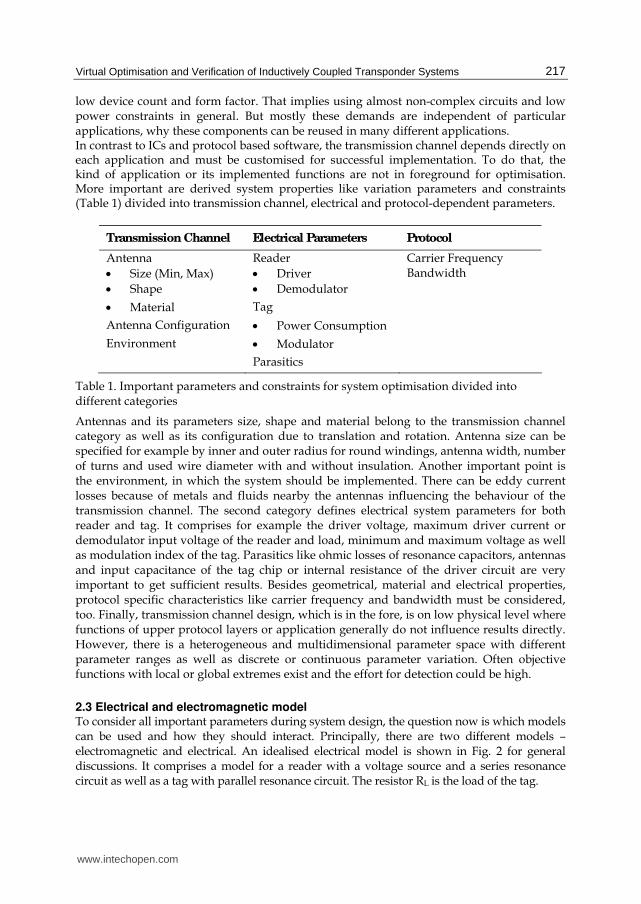
low device count and form factor. That implies using almost non-complex circuits and low power constraints in general. But mostly these demands are independent of particular applications, why these components can be reused in many different applications. In contrast to ICs and protocol based software, the transmission channel depends directly on each application and must be customised for successful implementation. To do that, the kind of application or its implemented functions are not in foreground for optimisation. More important are derived system properties like variation parameters and constraints (Table 1) divided into transmission channel, electrical and protocol-dependent parameters.

Transmission Channel Electrical Parameters Protocol

Antenna Reader Carrier Frequency

• Size (Min, Max) • Driver Bandwidth

• Shape • Demodulator

• Material Tag

Antenna Configuration • Power Consumption

Environment • Modulator

Parasitics

Table 1. Important parameters and constraints for system optimisation divided into different categories

Antennas and its parameters size, shape and material belong to the transmission channel category as well as its configuration due to translation and rotation. Antenna size can be specified for example by inner and outer radius for round windings, antenna width, number of turns and used wire diameter with and without insulation. Another important point is the environment, in which the system should be implemented. There can be eddy current losses because of metals and fluids nearby the antennas influencing the behaviour of the transmission channel. The second category defines electrical system parameters for both reader and tag. It comprises for example the driver voltage, maximum driver current or demodulator input voltage of the reader and load, minimum and maximum voltage as well as modulation index of the tag. Parasitics like ohmic losses of resonance capacitors, antennas and input capacitance of the tag chip or internal resistance of the driver circuit are very important to get sufficient results. Besides geometrical, material and electrical properties, protocol specific characteristics like carrier frequency and bandwidth must be considered, too. Finally, transmission channel design, which is in the fore, is on low physical level where functions of upper protocol layers or application generally do not influence results directly. However, there is a heterogeneous and multidimensional parameter space with different parameter ranges as well as discrete or continuous parameter variation. Often objective functions with local or global extremes exist and the effort for detection could be high.

2.3 Electrical and electromagnetic model To consider all important parameters during system design, the question now is which models can be used and how they should interact. Principally, there are two different models – electromagnetic and electrical. An idealised electrical model is shown in Fig. 2 for general discussions. It comprises a model for a reader with a voltage source and a series resonance circuit as well as a tag with parallel resonance circuit. The resistor RL is the load of the tag.

www.intechopen.com

Radio Frequency Identification Fundamentals and Applications, Design Methods and Solutions

218

Fig. 2. Idealised electrical model of a transponder system using inductive coupling

The transmission channel can be described by the impedance matrix

( )

R LR R R

T LT T T

V R j L j M I

V j M R j L I

ω ωω ω+ −⎡ ⎤ ⎡ ⎤ ⎡ ⎤=⎢ ⎥ ⎢ ⎥ ⎢ ⎥− +⎣ ⎦ ⎣ ⎦ ⎣ ⎦ , (1)

where VR and VT are the voltages over the antennas. IR and IT are the currents through the antennas. For system design of passive tags, two objective functions are important. These are the energy range and the transponder signal range (Finkenzeller, 2007). Energy range means the maximal distance between reader and tag, where the tag can extract enough energy from the field. Transponder signal range means the maximal distance, where the reader can receive data error-free from the tag. The sensitivity of the demodulator is very important for the transponder signal range. The goal is that energy range and transponder signal range exceed the required minimum link distance after system optimisation. To evaluate both energy range and transponder signal range, two objective functions can be used on the electrical level. These are the transponder voltage (2) and the demodulator input voltage (3) (Deicke et al., 2008a).

2

22 ( )

R LT

L LTLT L T

T

j MI RV

R RR R L

L

ωωω

= ⎛ ⎞+ +⎜ ⎟⎝ ⎠ (2)

[ ]0

,

1 1

Re ( ) Re ( )RR R

R L R L Mod

V V RZ Z Z Z

⎛ ⎞Δ = −⎜ ⎟⎜ ⎟⎡ ⎤⎣ ⎦⎝ ⎠ (3)

The real part of the impedance ZR is

[ ] ( )2

2 2

( )Re

( ) ( )R R LR LT L

LT L T

MZ R R R Z

R Z L

ωω= + + +− − + . (4)

ZL is the parallel connection of CT and RL. ZL,Mod is the parallel connection of CT and RL,Mod. Whereby, RL,Mod is the load resistance during modulation. Furthermore, there are constraints on the electrical model. These are the quality factor of the reader (5) and the transponder (6). Generally, the quality factor is defined by the quotient of resonance frequency and bandwidth.

www.intechopen.com

Virtual Optimisation and Verification of Inductively Coupled Transponder Systems

219

0 RR

LR R

LQ

R R

ω= + (5)

0

2 4 2 2 20

2

2 4

T LT

L L LT L T L

L RQ

R R R R L R

ωω= + − − (6)

Considering equation (1) to (6) and the discussion in previous sections, there are many

different variables that influence VT and ΔVRR. On the one side there are electrical parameters characterising the transmission channel that depend on geometrical dimensions, antenna configuration, antenna material and eddy current losses due to fluids or metals nearby antennas. These parameters must be calculated by an electromagnetic model and forwarded to the electrical model. If magnetic materials like ferrite cores or ferromagnetic plates are placed inside or nearby antennas, magnetic field strength or antenna current must also be considered because of saturation. Then, there is an additional loop-back between electrical and electromagnetic model. On the other side there are electrical components of resonance circuits like RR, CR and CT that depend on antenna and transmission channel parameters as well as system constraints like bandwidth and quality factor. It follows that there is no closed solution available that takes into account both electrical and electromagnetic model. Because of that, manual optimisation is very difficult for experienced designers, as well. An exhausted search in that large multidimensional parameter space is not possible mostly because of considering a vast number of possibilities that would result in a lack of time. On manual optimisation only few solutions can be verified. And as a result, it is not really sure if the solution found, is the optimum for a particular application or not. That means the quality of the result can not be estimated in a sufficient way.

2.4 Current approaches and its bottlenecks For RFID system dimensioning and analysis, different approaches had been discussed in literature. The selection of an adequate modelling approach depends on target-oriented use of variation parameters for design and optimisation. There are algebraic and numerical solutions in general. A well known work is (Grover, 2004) where many approximated formulas are collected to calculate self and mutual inductance for many different coil types. Using the approximated formulas for the electrical level from the application note (Roz, 1998) in combination with that work, simple system analysis can be done with an existing transmission channel including antennas and antenna configuration. Youbok introduced with (Youbok, 2003) a more detailed application note including formulas for most common antenna shapes and basic electrical circuits. For some standardised systems including co-axial antennas, no additional literature is necessary. Another interesting approach is discussed in (Finkenzeller, 2007) where a solution is presented to find the optimum antenna radius of reader for given read range and constant coil current. The reason is if the antenna radius is too large, the field strength is too low even at a distance of 0 between reader and tag antenna. And in the other way around, if the radius is too small, there is high field strength at distance 0, but it falls in proportion to x3 from nearby the reader antenna. So, Finkenzeller explains that radius R and read range x should have the relation

2xR = . (7)

www.intechopen.com

Radio Frequency Identification Fundamentals and Applications, Design Methods and Solutions

220

A question, that was not discussed, is if that formula is always true in free air independent of tag load or tag antenna size and shape. Mostly, it should not work in metal or fluid environments. Another interesting approach also explained in (Finkenzeller, 2007) is to find the minimum field strength at tag side to power a passive tag. Therefore, the mutual inductance M in equation (2) is replaced by a simple approximation using magnetic field strength H. Then the equation is solved for H. After that the minimum magnetic field strength Hmin can be estimated by defining a minimum tag voltage VT and a load resistance RL. With that result, the designer is able to dimension the reader of a system without any further relation to the tag side. An independent development of both reader and tag is possible if Hmin is constant. That approach seems to be good for basic analysis and optimisation if the antennas and the antenna configuration are well known and less accuracy is accepted. If antennas are unknown at the beginning of system design like it is the case for many new industrial or medical applications, it is difficult to find an optimised system. One point, that would also impede the use of that approach, is, that electromagnetic and electrical model are mixed and used in one step. So, it is really hard to implement more model details in that closed formula even to increase accuracy. And there is also no numerical solver that can be used for such a mixed approach. It can not be considered in that way if data transfer works from tag to reader or not, because even formulas for simple models will be very complex and difficult to handle. Finally, that approach only helps to optimise energy range. Besides these approaches with a reduced abstraction level, modelling using numerical methods is another way to increase model accuracy and to finally find better solutions. Therefore, specific computer-aided tools are used, like it is also done for many other problems in physics or engineering. But many specific tools such as ANSYS (ANSYS, 2007), FEMM (Meeker, 2006) or Spice (Quarles et al., 2005) only provide comprehensive functionalities for analysis and optimisation on particular modelling levels like mechanical, electrical or electromagnetic. Heterogeneous systems can not be analysed or optimised with one tool. Another possibility for analysis and optimisation is the use of modelling languages like VHDL-AMS or Verilog-A. These are used to model physical behaviour such as acoustic, electrical, magnetic, mechanical, optical or thermal. Interactions between different modelling levels can be considered as well. Another advantage in comparison to numerical solvers like ANSYS is that modelling languages are standardised. Thus it can be used independent of a particular simulator. A disadvantage is that detailed models are very complex and handling these complex models is often not as good as using numerical solvers. Two approaches using standardised modelling languages are explained in (Beroulle, 2003) and (Soffke, 2007). Beroulle uses VHDL-AMS to model a transponder system on system level with a carrier frequency of 2.45 GHz to validate system performance. Soffke takes a similar approach for system analysis. He uses Verilog-A to model an inductively coupled transponder system. System optimisations are done manually. That means, found solutions can be close to an optimum, but it can not be evaluated easily if it is the case. Mostly it remains a big uncertainty. All these approaches have in common not to be a good choice for system analysis and optimisation considering the whole transponder system and considering enough details in electrical and electromagnetic models to get sufficient results. Either it can be used for system analysis or to analyse parts of a whole system in detail without regard to interactions of other parts. Additionally, system optimisation is not described to find best solutions for different usage scenarios. Thus it is assumed to do it manually with all restrictions discussed above.

www.intechopen.com

Virtual Optimisation and Verification of Inductively Coupled Transponder Systems

221

3. Virtual design approach

3.1 Objectives From discussions above, objectives are derived for a virtual design approach that can be used for active and passive inductively coupled transponder systems. There, the focus is on antennas, transmission channels and its effects on the electrical level. Reader or tag antenna or both should be optimised dependent on application-specific requirements like geometrical, material or electrical properties and regarding whole system behaviour. Interactions between electrical and electromagnetic level should also be considered. During optimisation, a multidimensional and automatic parameter variation should be possible using adapted optimisation algorithm to get really optimised solutions and results with good quality. Besides pure optimisation, transponder systems should be analysed for different usage scenarios and different environments. Additionally, coaxial and non-coaxial antennas should be considered. That implies to move and rotate a tag in space for analysing operating range. To do that comprehensive analysis and optimisation, different model types should be selectable to choose between model accuracy, calculation time and possible model details like adding metal plates, for example. Finally, the goal is to make available a first system success design approach. This means that the first solution meets the requirements and can be used in practice without further extensive prototyping.

3.2 Design approach These objectives were realised in a stand-alone software tool called Transponder Calculation Tool (TransCal) and introduced in (Deicke et al., 2008b). It was developed by the Fraunhofer IPMS. TransCal comprises different known solvers for electrical and electromagnetic models (Fig. 3.). These are closed formulas for electrical model and for ohmic losses of antennas including skin effect and proximity effect (Deicke et al., 2008a). Additionally, there is an adapted Neumann formula used for high speed calculation of self and mutual inductance for coaxial and rotated antennas. And there are links to external numerical solvers like FastHenry (Kamon et al., 1996) and Spice (Quarles et al., 2005). FastHenry is a 3D electromagnetic solver based on the Partial Element Equivalent Circuit method. It can be used to model arbitrary antenna configurations, 3D antennas or additional conductive structures nearby the antennas like metal plates or even metal rims to analyse transponder systems in a car or truck wheel, for example.

Fig. 3. Design approach for TransCal

Besides these algorithms needed for detailed modelling on both levels, a framework is used to implement algorithms for analysis, optimisation and model coupling to form a system simulation. The framework bases on C/C++ in connection with Microsoft Foundation

www.intechopen.com

Radio Frequency Identification Fundamentals and Applications, Design Methods and Solutions

222

Classes to get a MS Windows compliant software tool with an appropriate graphical user interface. TransCal comprises five components like it is shown in the block diagram of Fig. 4. The analyser/optimiser module analyses and optimises different transponder systems using parameter variations and search algorithms. Furthermore, an automated model generator reorganises and adapts imported user defined netlists and generates antenna models as well as additional conductive structures nearby antennas. The model coupling module controls and synchronises different internal analytical algorithms and external numerical solvers selected by user.

Fig. 4. Block diagram of TransCal

3.3 Input/Output parameters and Initialisation The input of several user defined design tasks and the output of results are done with graphical user interface. Input parameters are geometrical and material properties of the antennas, variation ranges for optimisation and analysis as well as electrical properties. General settings for optimisation, analysis as well as used solvers can be made, too. The results are shown in a text-based output window and additionally stored in text files to provide the possibility for import in external data analysis and graphing tools. Fig. 5 shows a screenshot from TransCal with dialog-based input and text-based output. Each design is saved in a project file including all input settings and results to reopen and work on later. For defining parameter space, constant and variable parameters have to be set. Dimensions such as inner radius, outer radius and width of antenna or antenna type, number of turns and link distance are variable parameters. Considering the optimisation of one antenna, there are five degrees of freedom (DOF). And considering an optimisation of two antennas, there are nine DOF. As a result, a five- or nine-dimensional parameter space must be used. That seems to be very complicated and time consuming for most optimisation algorithms. An advantageous modification of that parameter space could be helpful to solve that optimisation task more efficiently. The reduction of variation parameters is to the fore. Principally, the variation of antenna geometry can be done by varying the number of turns if the antenna type is defined. Additionally, a constant fill factor has to be assumed. That is done by defining an outer diameter of the used wire including conductor and insulation. Using that substitution, the number of DOF can be reduced. Considering one antenna, the parameter space is reduced to one dimension assuming a constant link distance. And considering two antennas, the parameter space is reduced to two. If the link distance is variable, the number of DOF is increased by one. Considering objective functions VT and

www.intechopen.com

Virtual Optimisation and Verification of Inductively Coupled Transponder Systems

223

Fig. 5. Graphical user interface of TransCal with dialog-based input and text-based output

ΔVRR versus the number of turns, the characteristic of these functions is concave. That can be used later to simplify optimisation process, too. Subsequent to the definition of variation parameters, the generation of the n-dimensional

mesh is done. The parameter space has discrete values excluding link distance. Each node of

the mesh corresponds to a transponder system comprising a complete parameter set.

3.4 Optimisation and analysis Looking from implementation side, optimisation and analysis are closely related to each

other in general. The main difference is in generating new input parameters for system

simulation. On system analysis, all defined nodes must be considered. Instead, there is a

bigger parameter space on optimisation in general. Therefore, a more efficient algorithm is

needed to consider as few as possible nodes during that process to reduce overall

calculation time. The general flow, that was adapted from the well known simulation-based

optimisation approach (Carson & Maria, 1997), is shown in Fig. 6. The analyser/optimiser

module generates a new parameter set. First, electrical parameters of the transmission

channel are calculated using an electromagnetic solver. These are the inductance and ohmic

losses of the antennas as well as the mutual inductance. The impedance matrix is imported

in the electrical circuit subsequently. After additional adaptations of resonance capacitors

and quality factors, the objective functions VT and ΔVRR are calculated and imported in the

analyser/optimiser module. There, the results are evaluated and a new parameter set is

output. For optimisation, that loop is repeated until an optimised solution will be found for

a given parameter space. Calculation of transmission channel and electrical circuit is

controlled by the coupling module.

www.intechopen.com

Radio Frequency Identification Fundamentals and Applications, Design Methods and Solutions

224

Fig. 6. Simulation-based flow for analyser and optimiser

During system optimisation the goal is to find an optimal parameter set for any particular application with a minimum amount of computing resources and time. Therefore, it is desired that not all possibilities are evaluated explicitly. Especially with complicated and heterogeneous systems, optimisation could be a challenging part. Using simulation-based optimisation, all nodes must be found that meet defined constraints for objective functions. Fig. 7 depicts an example, where all systems are looked for that met constraints for objective

functions at a constant link distance. With that contour plot objective functions VT and ΔVRR are shown over the number of turns for reader NR and tag NT. The dash-point line is the equipotential line for the minimum transponder voltage VT,min. All nodes on the left hand side have a tag voltage that is at least the minimum value. The dashed line is the equipotential line for the minimum demodulator input voltage VRR,min. All nodes enclosed with that line have a demodulator input voltage that is at least the minimum value. The intersection of both areas shows all transponder systems that fulfil requirements for energy

Fig. 7. 2-dimensional mesh for an optimisation task and marked sections where objective

functions VT and ΔVRR meet requirements

www.intechopen.com

Virtual Optimisation and Verification of Inductively Coupled Transponder Systems

225

range and transponder signal range at a given link distance. For that design example, these systems are optimal solutions. If the intersection comprises only one node, that node defines the system with maximum link distance. Applying introduced simplifications for variation parameters, the objective functions are concave. Because of that, robust and simple gradient based search algorithm and logical operations are used to find the intersection. To find the node with maximum link distance, an additionally root finding algorithm was implemented. So, the overall optimisation task is divided into different steps using different simple and robust algorithms. In addition to that advanced optimisation method, a brute force method was implemented that considers all nodes available. Many design examples had shown that calculation time of the advanced method is less than 4% of the brute force method.

3.5 Model coupling The coupling module controls and synchronises different calculation types selected by user before starting analysis or optimisation. There are internal closed formulas and additionally external numerical solvers that can be selected for each modelling level to adjust used model accuracy and calculation time (Fig. 8). On the one side, it is possible only to use internal closed formulas and analytical algorithms to speed up calculation. Thereby, less accuracy is accepted. And on the other side, external numerical solvers can be used for both electrical and electromagnetic model to get best accuracy. The communication between TransCal and these external solvers are done using command and result files. At the moment, FastHenry and Spice can be used. But if necessary, other simulators can be connected, too. A third way is to mix internal algorithm and external solvers like it is shown in an example later.

Fig. 8. Model coupling module and connected solvers

The model for FastHenry simulator is generated by model generator of TransCal for each simulation step, because of changing antenna geometry. Besides calculation of coaxial antennas in free air, FastHenry additionally has the possibility to model non-coaxial antennas concerning translation and rotation as well as 3D antennas. Furthermore, metal plates inside or under each antenna as well as car or truck rims can be modelled regarding its influence on transmission channel. If other conductive structures should be used in models, model generator must be extended before. That can not be done by user. Using Spice, different user defined netlists can be imported by TransCal to provide the possibility to add particular components as well as to analyse different circuit concepts for reader and tag. The electrical model is focused on low level such as transmission channel,

www.intechopen.com

Radio Frequency Identification Fundamentals and Applications, Design Methods and Solutions

226

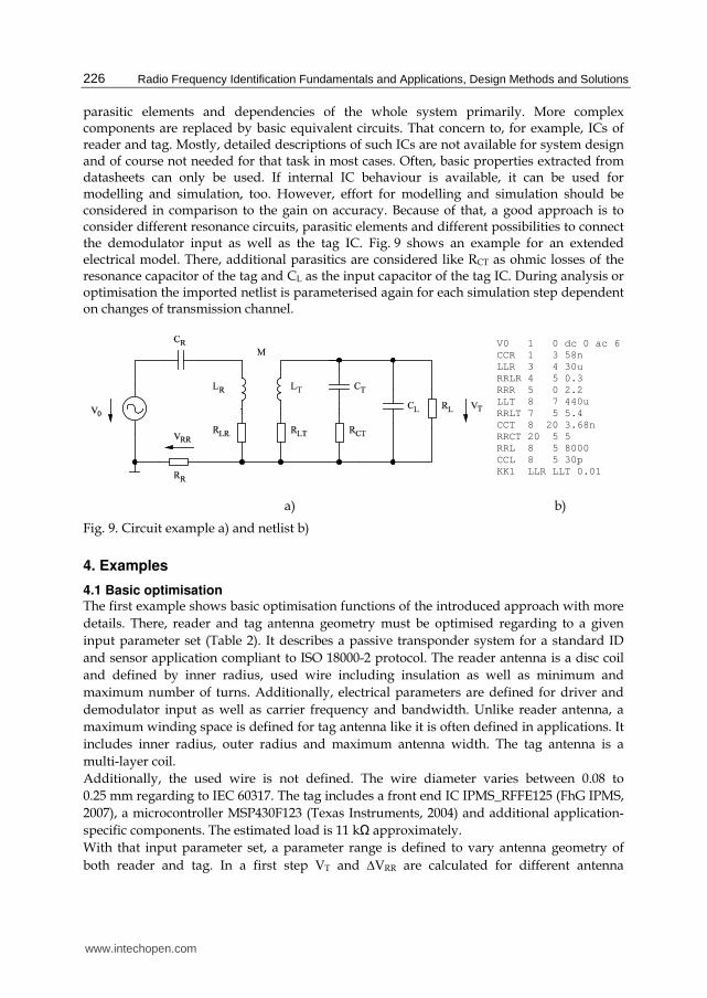
parasitic elements and dependencies of the whole system primarily. More complex components are replaced by basic equivalent circuits. That concern to, for example, ICs of reader and tag. Mostly, detailed descriptions of such ICs are not available for system design and of course not needed for that task in most cases. Often, basic properties extracted from datasheets can only be used. If internal IC behaviour is available, it can be used for modelling and simulation, too. However, effort for modelling and simulation should be considered in comparison to the gain on accuracy. Because of that, a good approach is to consider different resonance circuits, parasitic elements and different possibilities to connect the demodulator input as well as the tag IC. Fig. 9 shows an example for an extended electrical model. There, additional parasitics are considered like RCT as ohmic losses of the resonance capacitor of the tag and CL as the input capacitor of the tag IC. During analysis or optimisation the imported netlist is parameterised again for each simulation step dependent on changes of transmission channel.

V0 1 0 dc 0 ac 6 CCR 1 3 58n LLR 3 4 30u RRLR 4 5 0.3 RRR 5 0 2.2 LLT 8 7 440u RRLT 7 5 5.4 CCT 8 20 3.68n RRCT 20 5 5 RRL 8 5 8000 CCL 8 5 30p KK1 LLR LLT 0.01

a) b)

Fig. 9. Circuit example a) and netlist b)

4. Examples

4.1 Basic optimisation The first example shows basic optimisation functions of the introduced approach with more

details. There, reader and tag antenna geometry must be optimised regarding to a given

input parameter set (Table 2). It describes a passive transponder system for a standard ID

and sensor application compliant to ISO 18000-2 protocol. The reader antenna is a disc coil

and defined by inner radius, used wire including insulation as well as minimum and

maximum number of turns. Additionally, electrical parameters are defined for driver and

demodulator input as well as carrier frequency and bandwidth. Unlike reader antenna, a

maximum winding space is defined for tag antenna like it is often defined in applications. It

includes inner radius, outer radius and maximum antenna width. The tag antenna is a

multi-layer coil.

Additionally, the used wire is not defined. The wire diameter varies between 0.08 to

0.25 mm regarding to IEC 60317. The tag includes a front end IC IPMS_RFFE125 (FhG IPMS,

2007), a microcontroller MSP430F123 (Texas Instruments, 2004) and additional application-

specific components. The estimated load is 11 kΩ approximately.

With that input parameter set, a parameter range is defined to vary antenna geometry of

both reader and tag. In a first step VT and ΔVRR are calculated for different antenna

www.intechopen.com

Virtual Optimisation and Verification of Inductively Coupled Transponder Systems

227

geometries at minimum link distance (Fig. 10). The wire diameter of tag antenna is 0.2 mm

in that case. Maximum values for VT and ΔVRR are not in the same region of parameter

space. So, the system with maximum transponder voltage or maximum demodulator input

voltage is not the system with maximum link distance.

Table 2. Input parameter set for reader and tag

a) b)

Fig. 10. Tag voltage VT a) and demodulator input voltage ΔVRR b) vs. number of turns for reader and tag antenna at a fixed link distance

In a next step both antennas and system setup are optimised for maximum link distance

considering different wire diameters for tag antenna. The number of windings varies

between 21 and 22 for reader antenna, but there is no direct influence from wire diameter.

Fig. 11 a) shows the impedance of the tag antenna over the wire diameter for a constant

maximum winding space. The impedance for maximum link distance decreases with

www.intechopen.com

Radio Frequency Identification Fundamentals and Applications, Design Methods and Solutions

228

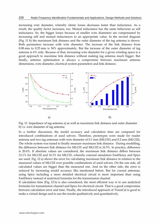
increasing wire diameter, whereby ohmic losses decreases faster than inductance. As a

result, the quality factor increases, too. Mutual inductance has the same behaviour as self

inductance. So, the bigger losses because of smaller wire diameters are compensated by

increasing self and mutual inductances to an appropriate value. In the second diagram

(Fig. 11 b) the maximum link distance and the outer diameter of the tag antenna is shown.

Both parameters increase with wire diameter. The increase of the link distance from

0.08 mm to 0.25 mm is 34% approximately. But the increase of the outer diameter of tag

antenna is 6% only. Because of that, increasing wire diameter for a given winding space is a

good approach to maximise link distance without making tag antenna much bigger. But

finally, antenna optimisation is always a compromise between maximum antenna

dimensions, wire diameter, electrical system parameters and link distance.

a) b)

Fig. 11. Impedance of tag antenna a) as well as maximum link distance and outer diameter b) vs. wire diameter of tag antenna

In a further discussion, the model accuracy and calculation time are compared for

introduced combinations of used solvers. Therefore, prototypes were made for reader

antenna and two tag antennas with wire diameter of 0.1 mm (MLC01) and 0.2 mm (MLC02).

The whole system was tuned to finally measure maximum link distance. During modelling,

the difference between link distance for MLC01 and MLC02 is 16.5%. In practice, difference

is 20.4%. If absolute values are considered, the maximum link distance differs between

12.1% for MLC02 and 16.3% for MLC01, whereby external simulators FastHenry and Spice

are used. Fig. 12 a) shows the error for calculating maximum link distance in relation to the

measured values of MLC02 over possible combinations of used solvers. On the one side, all

calculated values are bigger than the measured one. And on the other side, the error is

reduced by increasing model accuracy like mentioned before. But for coaxial antennas,

using Spice including a more detailed electrical circuit is more important than using

FastHenry instead of analytical formulas for the transmission channel.

If calculation time (Fig. 12 b) is also considered, the most efficient way is to use analytical

formulas for transmission channel and Spice for electrical circuit. That is a good compromise

between calculation error and time. Finally, the introduced approach of TransCal is good to

make a virtual design and to use the results qualitatively and quantitatively.

www.intechopen.com

Virtual Optimisation and Verification of Inductively Coupled Transponder Systems

229

a) b)

Fig. 12. Calculated link distance in relation to measured a) and calculation time b) vs. possible combinations of used solvers

4.2 3D antenna – dimensioning and analysis Inductively coupled transponder systems are mostly analysed and optimised using coaxial antennas. That approach is simple to use, but it is not sufficient for many applications and its operating range or coverage. Because of that, analysis of tag rotation and translation is important, too. In that section, analysis of rotation is in the fore. Standard antennas have a limited coverage. However, 3D antennas with three coils assigned in perpendicular to each other (Fig. 13), seem to have a better one. But a question is if 3D antennas will provide power supply and communication for arbitrary rotation or not. Answers can be found by making some analysis using TransCal.

Fig. 13. 3D antenna with perpendicular coils in the xy plane, the xz plane and the yz plane of a Cartesian coordinate system

For modelling and optimisation of practical 3D antennas, different design constraints can be used. The primary goal is to find a good approximation for geometrical and electrical properties in comparison with a theoretical approach where three equal coils are used. Therefore, design constraints are constant maximum link distance or constant coil impedance. If the coils are optimised for constant impedance, the resonance circuits are equal and as a consequence production process simplifies. Additional constraints are overall dimensions of a 3D antenna that also influence the winding space of each coil.

www.intechopen.com

Radio Frequency Identification Fundamentals and Applications, Design Methods and Solutions

230

If 3D antennas are generated using constant maximum link distance, VT and ΔVRR must have the same values at the same link distance and same rotation approximately. Starting from the inner coil that is also called basic antenna, the coil in the xz plane must have an inner radius that is bigger than the outer radius of the basic antenna. In a second step, the coil in the yz plane is generated, whereby its inner radius is bigger than the outer radius of the coil in the xz plane. 3D antenna generation and optimisation is done by TransCal automatically before starting further analysis. For that example a 3D antenna is derived from MLC02. A model for FastHenry simulator is shown in Fig. 14.

Fig. 14. 3D antenna model for FastHenry simulator

The simulated coverage of the single antenna MLC02 and a derived 3D antenna are shown

in Fig. 15 over the rotation about the x axis (ϕ) and y axis (θ). Coverage means, where the functionality of the tag is ensured. There, the transponder voltage VT and the demodulator

input voltage ΔVRR exceeds the defined limits at a given link distance. The coverage of the

a) b)

Fig. 15. Coverage of a single antenna a) and a 3D antenna b) vs. rotation about x axis (ϕ) and y axis (θ)

www.intechopen.com

Virtual Optimisation and Verification of Inductively Coupled Transponder Systems

231

single antenna is symmetric and represents 20.8% of the considered parameter space approximately. In comparison, the 3D antenna has a coverage of 91.4% approximately. It is more than 4.5 times bigger than of the single antenna. If link distance is very small, it could be 100%. Finally, 3D antennas can be used to increase coverage if tag position is not defined or if tag is rotating during use. But in most cases, 3D antennas are not able to get full coverage during rotation.

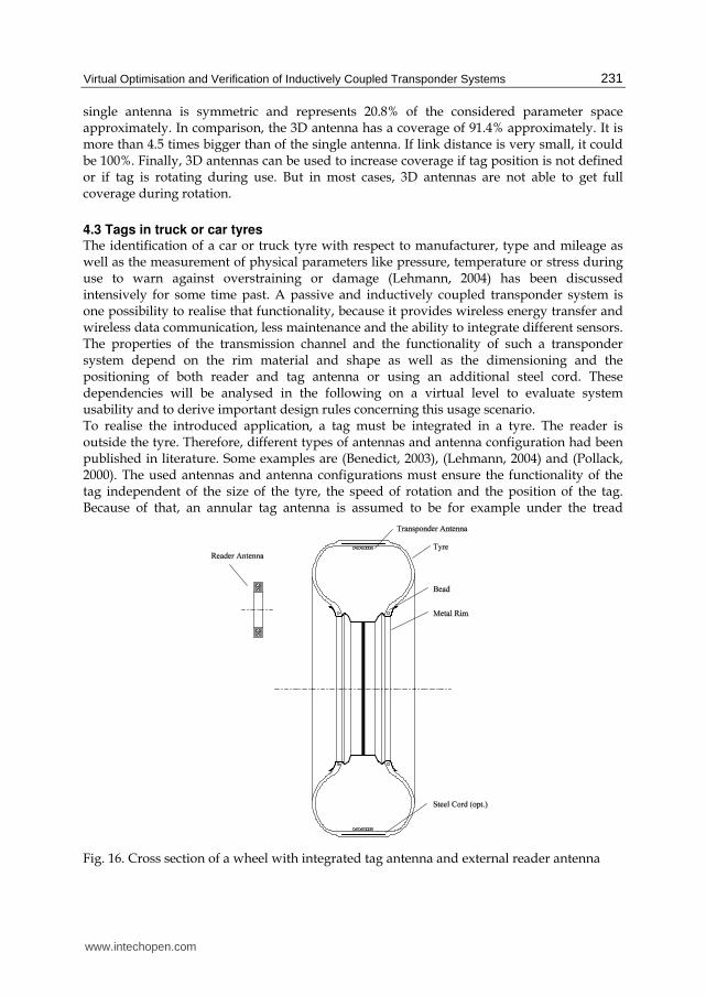
4.3 Tags in truck or car tyres The identification of a car or truck tyre with respect to manufacturer, type and mileage as well as the measurement of physical parameters like pressure, temperature or stress during use to warn against overstraining or damage (Lehmann, 2004) has been discussed intensively for some time past. A passive and inductively coupled transponder system is one possibility to realise that functionality, because it provides wireless energy transfer and wireless data communication, less maintenance and the ability to integrate different sensors. The properties of the transmission channel and the functionality of such a transponder system depend on the rim material and shape as well as the dimensioning and the positioning of both reader and tag antenna or using an additional steel cord. These dependencies will be analysed in the following on a virtual level to evaluate system usability and to derive important design rules concerning this usage scenario. To realise the introduced application, a tag must be integrated in a tyre. The reader is outside the tyre. Therefore, different types of antennas and antenna configuration had been published in literature. Some examples are (Benedict, 2003), (Lehmann, 2004) and (Pollack, 2000). The used antennas and antenna configurations must ensure the functionality of the tag independent of the size of the tyre, the speed of rotation and the position of the tag. Because of that, an annular tag antenna is assumed to be for example under the tread

Fig. 16. Cross section of a wheel with integrated tag antenna and external reader antenna

www.intechopen.com

Radio Frequency Identification Fundamentals and Applications, Design Methods and Solutions

232

(Fig. 16). The wheel and the tag antenna are coaxial. The annular antenna can be placed in the middle of the tyre, nearby the sidewall or the bead as well as on the rim or directly on a run-flat system (Continental, 2005; Rodgard, 2008). A steel cord can be placed inside the tyre optionally. The rim model can be generated by TransCal automatically using different variation parameters for a comprehensive analysis (Deicke et al., 2009). The transponder circuit can also be placed under the tread or inside the tyre. The reader antenna is outside and in parallel with the wheel. It is smaller than the tag antenna. So, the reader antenna can be positioned on the axle or on an advantageous position in the wheel case. A passive tag is used for identification and the integration of different sensors. Therefore, the ST1 transponder IC is used in a test setup. It provides an analogue 125 kHz RF front-end, a hard coded module to support low level ISO 18000-2 protocol functions, a 16-bit microcontroller core, RAM, flash, EEPROM, timers and several peripheral components to connect, for example, different sensors with an analogue or digital interface. Additionally, analogue and digital signal processing can be done on the tag side (Grätz et al., 2007). In the test setup, a combined pressure and temperature sensor MS5541 (Intersema, 2008) is connected to the ST1. So, the power consumption of the passive tag can be estimated to use it for analysing and optimisation of the whole system in the following. For system setup, the general input parameters of Table 3 are used.

Reader Tag

ri 31 mm ri 243 mm

b 10 mm b 11 mm

N 56 N 33

Antenna

Parameters

Type MLC Type TWS

V0 6.0 V VT,min 5.0 V

ΔVRR 0.01 V VT,max 5.5 V

f0 125 kHz RL 14 kΩ

Electrical

Parameters

bf 10 kHz RL,Mod 30 Ω

Table 3. Input parameter set for reader and tag of a tyre application

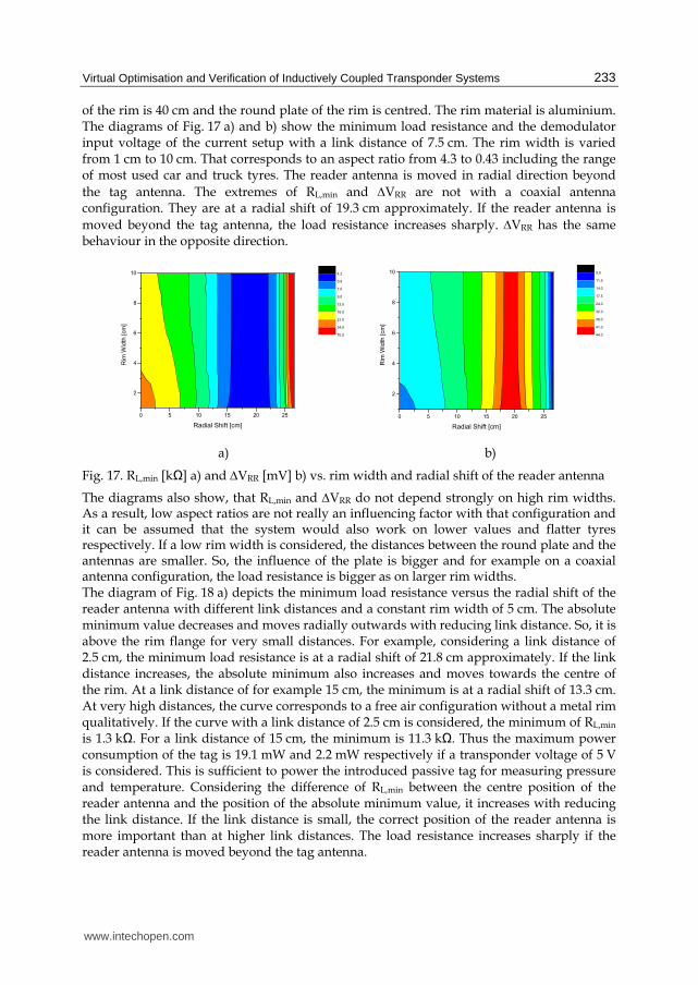
Both reader and tag antenna are optimised for maximum link distance in free air. Then, this optimised non-varying antenna setup is used to analyse and compare different rim configurations with and without steel cord. Later, both antennas can be optimised dependent on particular rim shape, size and material. The reader antenna is a multi-layer coil (MLC). It is smaller than the tag antenna that is a thin-walled solenoid (TWS). Additionally, Table 3 lists important electrical parameters of the reader and the tag. Two parameters are very important for system evaluation if a transponder system is analysed within a tyre. The first parameter is the minimum load resistance RL,min with a defined transponder voltage and link distance. Therewith, the maximum power consumption can be calculated to estimate which sensors and signal processing functions for measuring physical parameters can be implemented into the tag. The second parameter is the demodulator input voltage to determine if data communication is possible from tag to reader. For the first analysis below, an antenna configuration is used without a steel cord. Thereby, the rim width is varied to analyse different aspect ratios. Additionally, the reader antenna is moved in radial direction starting from a coaxial position. With this example, the diameter

www.intechopen.com

Virtual Optimisation and Verification of Inductively Coupled Transponder Systems

233

of the rim is 40 cm and the round plate of the rim is centred. The rim material is aluminium. The diagrams of Fig. 17 a) and b) show the minimum load resistance and the demodulator input voltage of the current setup with a link distance of 7.5 cm. The rim width is varied from 1 cm to 10 cm. That corresponds to an aspect ratio from 4.3 to 0.43 including the range of most used car and truck tyres. The reader antenna is moved in radial direction beyond

the tag antenna. The extremes of RL,min and ΔVRR are not with a coaxial antenna configuration. They are at a radial shift of 19.3 cm approximately. If the reader antenna is

moved beyond the tag antenna, the load resistance increases sharply. ΔVRR has the same behaviour in the opposite direction.

a) b)

Fig. 17. RL,min [kΩ] a) and ΔVRR [mV] b) vs. rim width and radial shift of the reader antenna

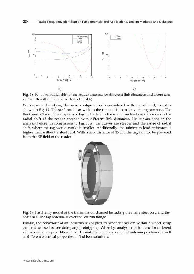
The diagrams also show, that RL,min and ΔVRR do not depend strongly on high rim widths. As a result, low aspect ratios are not really an influencing factor with that configuration and it can be assumed that the system would also work on lower values and flatter tyres respectively. If a low rim width is considered, the distances between the round plate and the antennas are smaller. So, the influence of the plate is bigger and for example on a coaxial antenna configuration, the load resistance is bigger as on larger rim widths. The diagram of Fig. 18 a) depicts the minimum load resistance versus the radial shift of the reader antenna with different link distances and a constant rim width of 5 cm. The absolute minimum value decreases and moves radially outwards with reducing link distance. So, it is above the rim flange for very small distances. For example, considering a link distance of 2.5 cm, the minimum load resistance is at a radial shift of 21.8 cm approximately. If the link distance increases, the absolute minimum also increases and moves towards the centre of the rim. At a link distance of for example 15 cm, the minimum is at a radial shift of 13.3 cm. At very high distances, the curve corresponds to a free air configuration without a metal rim qualitatively. If the curve with a link distance of 2.5 cm is considered, the minimum of RL,min is 1.3 kΩ. For a link distance of 15 cm, the minimum is 11.3 kΩ. Thus the maximum power consumption of the tag is 19.1 mW and 2.2 mW respectively if a transponder voltage of 5 V is considered. This is sufficient to power the introduced passive tag for measuring pressure and temperature. Considering the difference of RL,min between the centre position of the reader antenna and the position of the absolute minimum value, it increases with reducing the link distance. If the link distance is small, the correct position of the reader antenna is more important than at higher link distances. The load resistance increases sharply if the reader antenna is moved beyond the tag antenna.

www.intechopen.com

Radio Frequency Identification Fundamentals and Applications, Design Methods and Solutions

234

a) b)

Fig. 18. RL,min vs. radial shift of the reader antenna for different link distances and a constant rim width without a) and with steel cord b)

With a second analysis, the same configuration is considered with a steel cord, like it is shown in Fig. 19. The steel cord is as wide as the rim and is 1 cm above the tag antenna. The thickness is 2 mm. The diagram of Fig. 18 b) depicts the minimum load resistance versus the radial shift of the reader antenna with different link distances, like it was done in the analysis before. In comparison to Fig. 18 a), the curves are steeper and the range of radial shift, where the tag would work, is smaller. Additionally, the minimum load resistance is higher than without a steel cord. With a link distance of 15 cm, the tag can not be powered from the RF field of the reader.

Fig. 19. FastHenry model of the transmission channel including the rim, a steel cord and the antennas. The tag antenna is over the left rim flange.

Finally, the behaviour of an inductively coupled transponder system within a wheel setup can be discussed before doing any prototyping. Whereby, analysis can be done for different rim sizes and shapes, different reader and tag antennas, different antenna positions as well as different electrical properties to find best solutions.

www.intechopen.com

Virtual Optimisation and Verification of Inductively Coupled Transponder Systems

235

5. Conclusion

A first system success design approach for inductively coupled transponder systems was introduced. It bases on a software tool called TransCal. This tool can be used for system analysis and optimisation including automatic parameter variation and model generation. Many different customised designs including RFID technique can be solved in an easy and convenient way. Whereby, the focus is on transmission channel analysis, antenna design and its effects on the electrical level. During design process, the system is divided in an electromagnetic and an electrical model to consider necessary details in an appropriate way. Therefore, analytical algorithms are implemented in TransCal. Additionally, external numerical solvers can also be used to increase model accuracy. A model coupling module controls and synchronises internal and external solvers for these modelling levels to provide a system simulation finally. That functionality is used by an adapted simulation-based optimisation algorithm to find optimised solutions in a large, multidimensional and heterogeneous parameter space. In comparison to manual optimisation that only bases on human experience, better results concerning quality and quantity can be found within less amount of time. Using this approach, different usage scenarios can be considered such as coaxial or non-coaxial antennas including rotation and translation, different environments including eddy current losses as well as 3D antennas to increase tag coverage. Besides the theoretical introduction, three design examples are presented to show the advantages and limits of that approach. The first example introduces the basic optimisation process considering accuracy and calculation time, too. The second example is an analysis of 3D antennas versus single-coil antennas to compare system behaviour during rotation. In a third example a transponder system was implemented in a tyre for analysing different antenna positions. Finally, important questions like if a specific application would work using RFID technique or how to dimension and position antennas can be answered qualitatively and quantitatively on virtual level without doing a lot of prototyping. Additionally, it was shown that this design approach is less time consuming and expensive as well as provide better results for LF and HF systems to work with.

6. References

ANSYS Inc. (2007). ANSYS 11.0 User Manual. www.ansys.com Benedict, R.L. (2003). EPO Patent No. EP 1384603. European Patent Office Beroulle V., Khouri R., Vuong T. & Tedjini S. (2003). Behavioral Modelling and Simulation of

Antennas: Radio-Frequency Identification case study. BMAS Conference 2003, pp. 102-106, San Jose, USA, October 2003

Carson, Y., Maria, A. (1997). Simulation Optimization: Methods and Applications. Winter

Simulation Conference of the INFORMS Simulation Society, Atlanta, Georgia, December 1997

Continental AG. (2005). ContiSupportRing and Continental SSR. www.conti-online.com Deicke, F., Grätz, H. & Fischer, W.-J. (2008a). Combined System Analyses and Automated

Design of RFID Transponder Systems. IEEE International Conference on RFID, pp. 328-335, Las Vegas, USA, April 2008

Deicke, F., Grätz, H. & Fischer, W.-J. (2008b). Computer-Aided Design of Antennas, Transmission Channels and the Optimisation of Transponder Systems. RFID

SysTech 2008, pp. 32-41, June 2008

www.intechopen.com

Radio Frequency Identification Fundamentals and Applications, Design Methods and Solutions

236

Deicke, F., Grätz, H. & Fischer, W.-J. (2009). Analysis of Antennas for Sensor Tags Embedded in Tyres. RFID SysTech 2009, pp. 23-28, June 2009

FhG IPMS (2007). RFFE125 Datasheet. http://www.ipms.fraunhofer.de/en/ applications/sas-info.shtml

Finkenzeller, K. (2007). RFID Handbook. Fundamentals and Applications in Contactless Smart Cards and Identification. John Wiley & Sons Ltd.

Grätz, H, Heinig, A., Deicke, F. & Fischer, W.J. (2007). ST1 – ein freiprogrammierbarer Schaltkreis für 125 kHz Transponderlösungen. Mikrosystemtechnik-Kongress, Dresden, Germany, October 2007.

Grover, F. W. (2004). Inductance Calculations: Working Formulas and Tables. Reprinted in Dover Publications

International Electrical Commission (2005). IEC 60317 Specifications for particular types of winding wires. www.iec.ch

Intersema Sensoric SA (2008). MS5541-30C Datasheet. http://www.intersema.ch/ products/guide/calibrated/ms55341-30c/

Kamon, M., Smithhilser, C., White, J. (1996). FastHenry User’s Guide. http://www.fastfieldsolvers.com

Lehmann, J. (2004). WIPO Patent No. WO 2004/108439. World Intellectual Property Organization

Meeker, D. (2006). Finite Element Method Magnetics User’s Manual http://femm.foster-miller.net

Pollack, R.S. (2000). EPO Patent No. EP 1037755. European Patent Office Quarles, T., Pederson, D., Newton, R., Sangiovanni-Vincentelli, A. & Wayne, C. (2005). The

Spice Page. http://bwrc.eecs.berkeley.edu/Classes/IcBook/ SPICE/ Rodgard (2008). Pneumatic Tire Run-Flat Systems. http://www.rodgard.com/ mobility.htm Roz, T. & Fuentes, V. (1998). Using low power transponders and tags for RFID applications.

EM Microelectronic Marin SA Soffke O., Zhao P., Hollstein T. & Glesner M. (2007). Modelling of HF and UHF RFID

Technology for System and Circuit Level Simulations. RFID SysTech 2007 - ITG-

Fachbericht Vol. 203. Duisburg, Germany, July 2007. Texas Instruments (2004). MSP430x12x2 Datasheet. www.ti.com Youbok, L. (2003). Antenna Circuit Design for RFID Applications. Microchip Technology

Inc.

www.intechopen.com

Radio Frequency Identification Fundamentals and ApplicationsDesign Methods and SolutionsEdited by Cristina Turcu

ISBN 978-953-7619-72-5Hard cover, 324 pagesPublisher InTechPublished online 01, February, 2010Published in print edition February, 2010

InTech EuropeUniversity Campus STeP Ri Slavka Krautzeka 83/A 51000 Rijeka, Croatia Phone: +385 (51) 770 447 Fax: +385 (51) 686 166www.intechopen.com

InTech ChinaUnit 405, Office Block, Hotel Equatorial Shanghai No.65, Yan An Road (West), Shanghai, 200040, China

Phone: +86-21-62489820 Fax: +86-21-62489821

This book, entitled Radio Frequency Identification Fundamentals and Applications, Bringing Research toPractice, bridges the gap between theory and practice and brings together a variety of research results andpractical solutions in the field of RFID. The book is a rich collection of articles written by people from all overthe world: teachers, researchers, engineers, and technical people with strong background in the RFID area.Developed as a source of information on RFID technology, the book addresses a wide audience includingdesigners for RFID systems, researchers, students and anyone who would like to learn about this field. At thispoint I would like to express my thanks to all scientists who were kind enough to contribute to the success ofthis project by presenting numerous technical studies and research results. However, we couldn’t havepublished this book without the effort of InTech team. I wish to extend my most sincere gratitude to InTechpublishing house for continuing to publish new, interesting and valuable books for all of us.

How to referenceIn order to correctly reference this scholarly work, feel free to copy and paste the following:

Frank Deicke, Hagen Grätz and Wolf-Joachim Fischer (2010). Virtual Optimisation and Verification ofInductively Coupled Transponder Systems, Radio Frequency Identification Fundamentals and ApplicationsDesign Methods and Solutions, Cristina Turcu (Ed.), ISBN: 978-953-7619-72-5, InTech, Available from:http://www.intechopen.com/books/radio-frequency-identification-fundamentals-and-applications-design-methods-and-solutions/virtual-optimisation-and-verification-of-inductively-coupled-transponder-systems

© 2010 The Author(s). Licensee IntechOpen. This chapter is distributedunder the terms of the Creative Commons Attribution-NonCommercial-ShareAlike-3.0 License, which permits use, distribution and reproduction fornon-commercial purposes, provided the original is properly cited andderivative works building on this content are distributed under the samelicense.