Virtual Computational Camera

Changyin Zhou changyin@cs.columbia.edu

Columbia University, 1214 Amsterdam Ave, New York, NY 10027, USA

Keywords: computer camera, optics, light field

Abstract

In computational camera research, peopledesign unconventional optics to sample thelight field in a way that is radically differentfrom the traditional camera and preserve newforms of visual information for various appli-cations. When one has an idea of optics de-sign, it is very often that an evaluation basedon simulation has to be conducted first be-fore building a real system. However, how toquickly simulate an unconventional camera isoften a challenging problem even with profes-sional optical design software (e.g. Zemax).First, these software is designed for opticsresearches and usually do not support lightfield, which is a central concept in computa-tional camera research. Secondly, researchershave to spend plenty of time in designing de-tailed physical profiles of optical elements. Inthis project, we develop a framework of vir-tual computational camera for light field pro-cessing. With this framework, one can easilysimulate the light field processing of a virtualcomputational camera.

In the proposed framework, we formulatethree categories of optics, including lineartransform optics (lenses and prisms), dot-production optics (photomasks), and con-volution optics (diffusers and some phase-plates). We propose an efficient computationstrategy to render light fields at a decent res-olution.

1. Introduction

Computational cameras, which use new optics to maprays in the light field to pixels in an unconventional

Preliminary work. Under review by Prof. Peter Belhumeurand Jinwei Gu as a final project report of ComputationalPhotography, Spring 2009.

fashion, have attracted increasing attentions in recentyears(Nayar, 2006). Due to the unconventional op-tics, computational cameras can optically encode newand useful forms of visual information in the cap-tured image for the afterward interpretation. For ex-ample, researches show that a simple photomask canbe used in a camera for different purposes. (Levinet al., 2007) put an optimized mask at the apertureplane for the purpose of depth from defocus. (Zhou& Nayar, 2009) optimized different aperture patternsfor better performance of defocus deblurring. (Veer-araghavan et al., 2007) placed a planar photomask inthe optical path between the lens and sensor for lightfield acquisition. Besides, many other optics, such asprisms, phase-plates, lens arrays, diffusers, and so on,have also been widely used for a variety of applications(Lee et al., 1999)(Ng et al., 2005)(Dowski & Cathey,1995)(Garcıa-Guerrero et al., 2007).

People may notice that few of these computational de-signs are easy to implement. Actually it is not alwayspossible for one to open an lens and input somethinginside precisely. Before doing these, one may prefer toconduct a simulation to verify the design and optimizethe settings. One possible way is to use some pro-fessional optical design software (e.g. Zemax(Geary,2002)). With these professional software, one can de-sign the detailed profile of each optics and simulatehow rays will be processed. If the profiles are givenprecisely, a high precision output which perfectly fitsto the real result is expected. However, these opti-cal design software are not well designed for computa-tional camera researches.

First, these software do not support light field(Levoy& Hanrahan, 1996), a central concept in most com-putational researches. Some of them may be ableto ray trace a planar lambertian scene and simulatea limit resolution image, but to my best knowledge,none of them is able to simulate the imaging processof a general light field. Secondly, using these softwareforces researchers to spend plenty of time in designing

Virtual Computational Camera

detailed physics profiles of optical components. Al-though doing this may help to clarify the feasibilityissue at the very beginning, it might not be the righttime.

Also, it should be noted that for the 4D nature of lightfield and the complicated optics properties, in manycases, it is difficult or time consuming to write a sim-ulator from scratch. For example, in (Veeraraghavanet al., 2007), the authors proposed to place a mask inthe optical path. Intuitively, it is simple. However,most people may find it extremely difficult to simulatesuch a system. This is because human usually is notgood at thinking in a 4D space and because the sim-ulation algorithm is very tricky for the massive size of4D light field.

Our motivation is to build a framework of virtual com-putational camera, with which researchers can quicklyprototype their ideas and simulate how the systemswill work with any given light field. This simulation isgood for a concept verification or understanding beforeone really designs detailed physics profiles of optics orimplements a real system.

1.1. Design Purpose

To better serve researches in computational camera,the virtual computational camera will have the follow-ing properties:

• Light field based: all the processing should be per-formed on light field.

• Object oriented: users can simply define opticselements and indicate where to place, and do nothave to care too much about the detailed process-ing issues.

• Virtual: All the components are defined mathe-matically. Users do not have to worry about theimplementation issues at this stage.

• Reasonable Resolution and precision: We requirethe system to afford precise simulations at a rea-sonable resolution.

2. Related Work

Ray tracing (Glassner, 1989)(Levoy, 1990) is a popu-lar method widely used in graphics rendering and alsoin most optical design software. This method traceseach light through the pixel and computes how theray will be changed at every intersection to any ob-ject. Ray tracing is usually computational expensive,and therefore does not support light field processingwell.

Light field rendering using matrix optics (Ahren-berg & Magnor, 2006)(Georgeiv & Intwala, 2006) is amore effective rendering method for imaging. By mak-ing use of the matrix optics (Halbach, 1964)(Gerrard& Burch, 1994), this method propagates the opticstransform matrix instead of transforming the light fieldat each intersection, and therefore greatly reduces thecomputation cost. However, all the previous discus-sions are strictly constrained to a system that only hasmatrix optics, such as lenses and prisms. We will showthat many widely used optics, like photomasks and dif-fusers, cannot be formulated as ray transfer matrices.These methods cannot be applied once any non-matrixoptics is present in a camera.

In our work, we formulate three categories of optics,including linear transform optics (lenses, prisms), dotproduction optics (photomasks), and convolution op-tics (diffusers and some phase-plates). In addition, weshow how to efficiently render the light field when theyare presented together in a camera system. (Convolu-tion optics has not been discussed yet in the currentversion.)

3. Light Field and Camera

3.1. Light Field

A light field is a function that describes the amountof lights in every direction through every point in aspace(Wiki, 2009)(Levoy & Hanrahan, 1996). For aopen space, the light field is a 4D function or can bewritten as a 4D array in the discrete case. Thoughlight field can be generalized to include the temporaland spectrum dimension, we constrain ourselves to thetypical 4D light field in this project.

There are various parameterizations of 4D light field,among which the most common is the two-plane pa-rameterization shown in Figure 1 (a). In this project,a variant of UVST space shown in Figure 1(b) is usedto simplify the later light field analysis.

0

v

u

t

s

L(u, v, s, t)

0

v

u

0

0

s

t

L(u, v, s, t)

(a) (b)

0

v

u

t

s

L(u, v, s, t)

0

0

v

u

t

s

L(u, v, s, t)

0

v

u

0

0

s

t

L(u, v, s, t)

v

u

0

0

s

t

L(u, v, s, t)

(a) (b)

Figure 1. Parameterization of 4D Light Field. (a) Themost commonly used UVST parameterization; (b) Thevariant of UVST parameterization which is used in thispaper.

Virtual Computational Camera

3.2. Camera

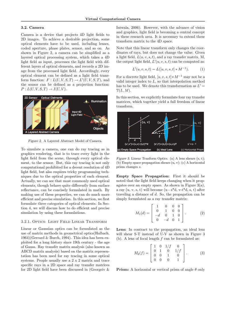
Camera is a device that projects 4D light fields to2D images. To achieve a desirable projection, someoptical elements have to be used, including lenses,coded aperture, phase plates, sensor, and so on. Asshown in Figure 2, a camera can be simplified as alayered optical processing system, which takes a 4Dlight field as input, processes the light field with dif-ferent layers of optical elements, and records a 2D im-age from the processed light field. Accordingly, everyoptical element can be defined as a light field trans-form function: F : L(U, V, S, T ) → L′(U, V, S, T ), andthe sensor can be defined as a projection function:P : L(U, V, S, T ) → I(U, V ).

Optical Elelments

A Layered Abstract Camera

2D Sensor

Input 4D

Light Field

Illumination

Objects

Optical Elelments

A Layered Abstract Camera

2D Sensor

Input 4D

Light Field

Illumination

Objects

Figure 2. A Layered Abstract Model of Camera.

To simulate a camera, one can do ray tracing as ingraphics rendering, that is to trace every light in thelight field from the scene, through every optical ele-ment, to the sensor. But, this ray tracing is not onlycomputational prohibited for a decent resolution of 4Dlight field, but also requires tricky programming tech-niques due to the optical properties of each element.Actually, we can see that most commonly used opticalelements, though behave quite differently from surfacereflectance, can be concisely formulated in math. Bymaking use of these properties, we can do much moreefficient and precise simulation. In this section, we firstformulate three categories of optical elements. In Sec-tion 4, we will discuss how to do efficient and precisesimulation by using these formulations.

3.2.1. Optics: Light Field Linear Transform

Linear or Gaussian optics can be formulated as theuse of matrix methods in geometrical optics(Halbach,1964)(Gerrard & Burch, 1994). This idea has been ex-ploited for a long history since 19th century - the ageof Gauss. Ray transfer matrix analysis (also known asABCD matrix analysis) based on the matrix represen-tation has been used for ray tracing in some opticalsystems. People usually use a 2 x 2 matrix and tracespecific rays in a 2D space and ray transfer matricesfor 2D light field have been discussed in (Georgeiv &

Intwala, 2006). However, with the advance of visionand graphics, light field is becoming a central conceptin these research area. It is necessary to extend thesetransform matrix to the 4D space.

Note that this linear transform only changes the coor-dinates of rays, but does not change the value. Givena light field, L(u, v, s, t), and a ray transfer matrix, M,the output light field, L′(u, v, s, t) can be computed as:

L′(u, v, s, t) = L([u, v, s, t] ∗M−1). (1)

For a discrete light field, [u, v, s, t]∗M−1 may not be avalid integer index to L, so that interpolation methodhas to be used. We denote this transformation as L′ =T(L,M).

In this section, we explicitly formulate four ray transfermatrices, which together yield a full freedom of lineartransform.

(u, v)

s’=s-

f

(u, v)

(s’,t’)=(s,t)+(u,v)/f

(b) Ideal Lens

f

(u, v)

(s’,t’)=(s,t)+(u,v)/f

(b) Ideal Lens

(u, v)

d

(u’,v’)=(u,v)-(s,t)*d

(a) Empty Space Propagation

(u, v)

d

(u’,v’)=(u,v)-(s,t)*d

(a) Empty Space Propagation (c) Horizontal Prism

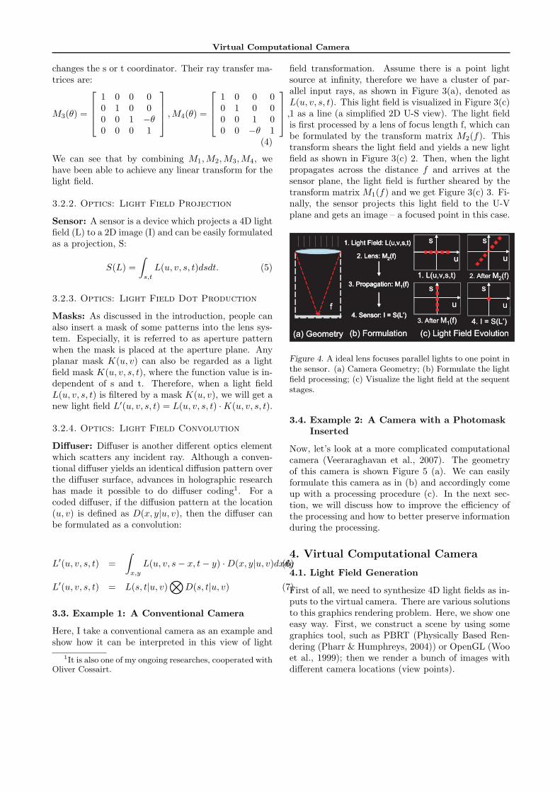
Figure 3. Linear Tranform Optics. (a) A lens shears (s, t);(b) Empty space propagation shears (u, v); (c) A horizontalprism changes s.

Empty Space Propagation: First it should benoted that the light field keeps changing when it prop-agates over an empty space. As shown in Figure 3(a),a ray (u, v, s, t) will become (u - s*d, v-t*d, s, t) aftertraveling a distance of d. So, the propagation can besimply formulated as a ray transfer matrix:

M1(d) =

1 0 0 00 1 0 0−d 0 1 00 −d 0 1

. (2)

Lens: In contract to the propagation, an ideal lenswill shear S-T instead of U-V as shown in Figure 3(b). A lens of focal length f can be formulated as:

M2(f) =

1 0 1/f 00 1 0 1/f0 0 1 00 0 0 1

. (3)

Prism: A horizontal or vertical prism of angle θ only

Virtual Computational Camera

changes the s or t coordinator. Their ray transfer ma-trices are:

M3(θ) =

1 0 0 00 1 0 00 0 1 −θ0 0 0 1

,M4(θ) =

1 0 0 00 1 0 00 0 1 00 0 −θ 1

,

(4)

We can see that by combining M1,M2,M3,M4, wehave been able to achieve any linear transform for thelight field.

3.2.2. Optics: Light Field Projection

Sensor: A sensor is a device which projects a 4D lightfield (L) to a 2D image (I) and can be easily formulatedas a projection, S:

S(L) =∫

s,t

L(u, v, s, t)dsdt. (5)

3.2.3. Optics: Light Field Dot Production

Masks: As discussed in the introduction, people canalso insert a mask of some patterns into the lens sys-tem. Especially, it is referred to as aperture patternwhen the mask is placed at the aperture plane. Anyplanar mask K(u, v) can also be regarded as a lightfield mask K(u, v, s, t), where the function value is in-dependent of s and t. Therefore, when a light fieldL(u, v, s, t) is filtered by a mask K(u, v), we will get anew light field L′(u, v, s, t) = L(u, v, s, t) ·K(u, v, s, t).

3.2.4. Optics: Light Field Convolution

Diffuser: Diffuser is another different optics elementwhich scatters any incident ray. Although a conven-tional diffuser yields an identical diffusion pattern overthe diffuser surface, advances in holographic researchhas made it possible to do diffuser coding1. For acoded diffuser, if the diffusion pattern at the location(u, v) is defined as D(x, y|u, v), then the diffuser canbe formulated as a convolution:

L′(u, v, s, t) =∫

x,y

L(u, v, s− x, t− y) ·D(x, y|u, v)dxdy(6)

L′(u, v, s, t) = L(s, t|u, v)⊗

D(s, t|u, v) (7)

3.3. Example 1: A Conventional Camera

Here, I take a conventional camera as an example andshow how it can be interpreted in this view of light

1It is also one of my ongoing researches, cooperated withOliver Cossairt.

field transformation. Assume there is a point lightsource at infinity, therefore we have a cluster of par-allel input rays, as shown in Figure 3(a), denoted asL(u, v, s, t). This light field is visualized in Figure 3(c)1 as a line (a simplified 2D U-S view). The light fieldis first processed by a lens of focus length f, which canbe formulated by the transform matrix M2(f). Thistransform shears the light field and yields a new lightfield as shown in Figure 3(c) 2. Then, when the lightpropagates across the distance f and arrives at thesensor plane, the light field is further sheared by thetransform matrix M1(f) and we get Figure 3(c) 3. Fi-nally, the sensor projects this light field to the U-Vplane and gets an image – a focused point in this case.

1. Light Field: L(u,v,s,t)

2. Lens: M2(f)

3. Propagation: M1(f)

4. Sensor: I = S(L’)

f

u

s

1. L(u,v,s,t)

u

s

2. After M2(f)

u

s

4. I = S(L’)

u

s

3. After M1(f)

(a) Geometry (b) Formulation (c) Light Field Evolution

1. Light Field: L(u,v,s,t)

2. Lens: M2(f)

3. Propagation: M1(f)

4. Sensor: I = S(L’)

1. Light Field: L(u,v,s,t)

2. Lens: M2(f)

3. Propagation: M1(f)

4. Sensor: I = S(L’)

f

u

s

1. L(u,v,s,t)

u

s

2. After M2(f)

u

s

4. I = S(L’)

u

s

3. After M1(f)

(a) Geometry (b) Formulation (c) Light Field Evolution

Figure 4. A ideal lens focuses parallel lights to one point inthe sensor. (a) Camera Geometry; (b) Formulate the lightfield processing; (c) Visualize the light field at the sequentstages.

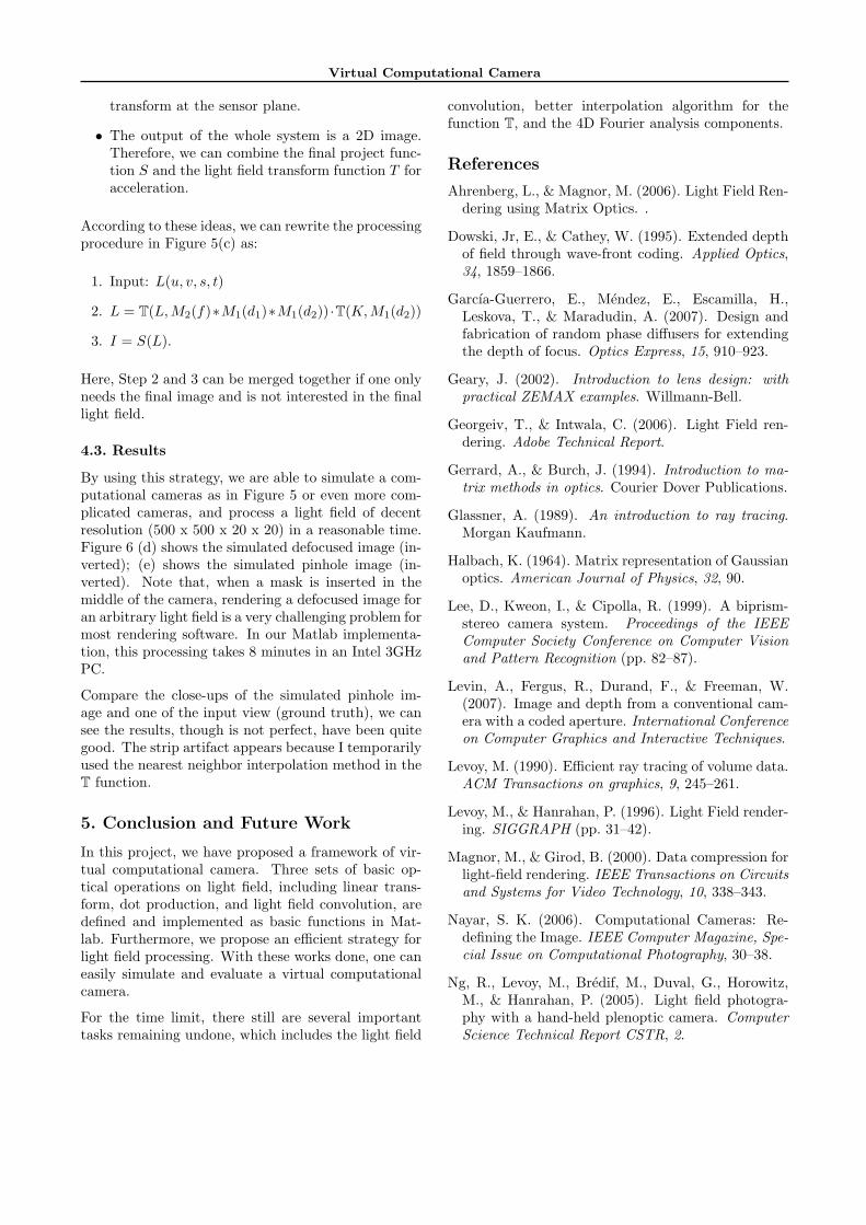
3.4. Example 2: A Camera with a PhotomaskInserted

Now, let’s look at a more complicated computationalcamera (Veeraraghavan et al., 2007). The geometryof this camera is shown Figure 5 (a). We can easilyformulate this camera as in (b) and accordingly comeup with a processing procedure (c). In the next sec-tion, we will discuss how to improve the efficiency ofthe processing and how to better preserve informationduring the processing.

4. Virtual Computational Camera

4.1. Light Field Generation

First of all, we need to synthesize 4D light fields as in-puts to the virtual camera. There are various solutionsto this graphics rendering problem. Here, we show oneeasy way. First, we construct a scene by using somegraphics tool, such as PBRT (Physically Based Ren-dering (Pharr & Humphreys, 2004)) or OpenGL (Wooet al., 1999); then we render a bunch of images withdifferent camera locations (view points).

Virtual Computational Camera

(c) Processing

1. Light Field: L(u,v,s,t)

2. Lens: M2(f)

3. Propagation: M1(d1)

6. Sensor: I = S(L)

(a) Geometry (b) Formulation

Mask d1

d2 5. Propagation: M1(d2)

4. Mask: K(u, v)

1. Input: L(u,v,s,t)

6. I = S(L)

3. L = t(L, M1(d1))

2. L = t(L, M2(f))

4. L = L . K

5. L = t(L, M1(d2))

(c) Processing

1. Light Field: L(u,v,s,t)

2. Lens: M2(f)

3. Propagation: M1(d1)

6. Sensor: I = S(L)

(a) Geometry (b) Formulation

Mask d1

d2 5. Propagation: M1(d2)

4. Mask: K(u, v)

1. Input: L(u,v,s,t)

6. I = S(L)

3. L = t(L, M1(d1))

2. L = t(L, M2(f))

4. L = L . K

5. L = t(L, M1(d2))

Figure 5. A camera with a planar photomask inserted inthe optical path. (a) Camera Geometry; (b) Formulateevery optical element

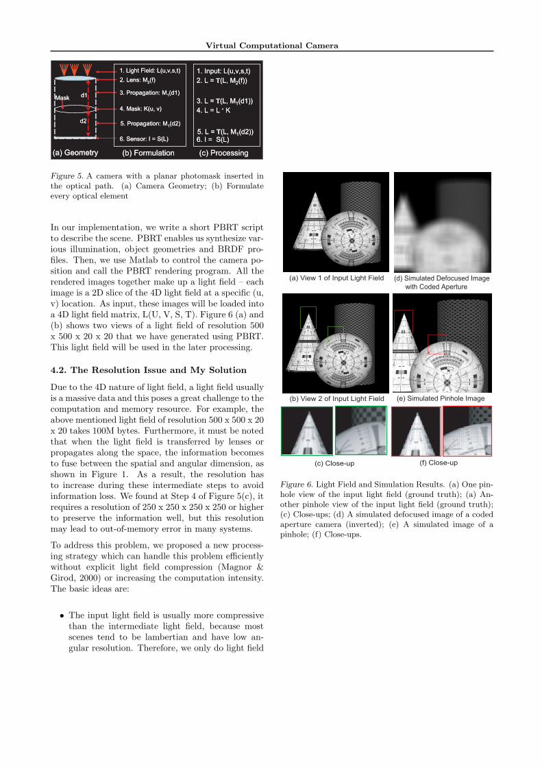
In our implementation, we write a short PBRT scriptto describe the scene. PBRT enables us synthesize var-ious illumination, object geometries and BRDF pro-files. Then, we use Matlab to control the camera po-sition and call the PBRT rendering program. All therendered images together make up a light field – eachimage is a 2D slice of the 4D light field at a specific (u,v) location. As input, these images will be loaded intoa 4D light field matrix, L(U, V, S, T). Figure 6 (a) and(b) shows two views of a light field of resolution 500x 500 x 20 x 20 that we have generated using PBRT.This light field will be used in the later processing.

4.2. The Resolution Issue and My Solution

Due to the 4D nature of light field, a light field usuallyis a massive data and this poses a great challenge to thecomputation and memory resource. For example, theabove mentioned light field of resolution 500 x 500 x 20x 20 takes 100M bytes. Furthermore, it must be notedthat when the light field is transferred by lenses orpropagates along the space, the information becomesto fuse between the spatial and angular dimension, asshown in Figure 1. As a result, the resolution hasto increase during these intermediate steps to avoidinformation loss. We found at Step 4 of Figure 5(c), itrequires a resolution of 250 x 250 x 250 x 250 or higherto preserve the information well, but this resolutionmay lead to out-of-memory error in many systems.

To address this problem, we proposed a new process-ing strategy which can handle this problem efficientlywithout explicit light field compression (Magnor &Girod, 2000) or increasing the computation intensity.The basic ideas are:

• The input light field is usually more compressivethan the intermediate light field, because mostscenes tend to be lambertian and have low an-gular resolution. Therefore, we only do light field

(d) Simulated Defocused Image

with Coded Aperture

(c) Close-up (f) Close-up

(a) View 1 of Input Light Field

(e) Simulated Pinhole Image(b) View 2 of Input Light Field

Figure 6. Light Field and Simulation Results. (a) One pin-hole view of the input light field (ground truth); (a) An-other pinhole view of the input light field (ground truth);(c) Close-ups; (d) A simulated defocused image of a codedaperture camera (inverted); (e) A simulated image of apinhole; (f) Close-ups.

Virtual Computational Camera

transform at the sensor plane.

• The output of the whole system is a 2D image.Therefore, we can combine the final project func-tion S and the light field transform function T foracceleration.

According to these ideas, we can rewrite the processingprocedure in Figure 5(c) as:

1. Input: L(u, v, s, t)

2. L = T(L,M2(f)∗M1(d1)∗M1(d2)) ·T(K, M1(d2))

3. I = S(L).

Here, Step 2 and 3 can be merged together if one onlyneeds the final image and is not interested in the finallight field.

4.3. Results

By using this strategy, we are able to simulate a com-putational cameras as in Figure 5 or even more com-plicated cameras, and process a light field of decentresolution (500 x 500 x 20 x 20) in a reasonable time.Figure 6 (d) shows the simulated defocused image (in-verted); (e) shows the simulated pinhole image (in-verted). Note that, when a mask is inserted in themiddle of the camera, rendering a defocused image foran arbitrary light field is a very challenging problem formost rendering software. In our Matlab implementa-tion, this processing takes 8 minutes in an Intel 3GHzPC.

Compare the close-ups of the simulated pinhole im-age and one of the input view (ground truth), we cansee the results, though is not perfect, have been quitegood. The strip artifact appears because I temporarilyused the nearest neighbor interpolation method in theT function.

5. Conclusion and Future Work

In this project, we have proposed a framework of vir-tual computational camera. Three sets of basic op-tical operations on light field, including linear trans-form, dot production, and light field convolution, aredefined and implemented as basic functions in Mat-lab. Furthermore, we propose an efficient strategy forlight field processing. With these works done, one caneasily simulate and evaluate a virtual computationalcamera.

For the time limit, there still are several importanttasks remaining undone, which includes the light field

convolution, better interpolation algorithm for thefunction T, and the 4D Fourier analysis components.

References

Ahrenberg, L., & Magnor, M. (2006). Light Field Ren-dering using Matrix Optics. .

Dowski, Jr, E., & Cathey, W. (1995). Extended depthof field through wave-front coding. Applied Optics,34, 1859–1866.

Garcıa-Guerrero, E., Mendez, E., Escamilla, H.,Leskova, T., & Maradudin, A. (2007). Design andfabrication of random phase diffusers for extendingthe depth of focus. Optics Express, 15, 910–923.

Geary, J. (2002). Introduction to lens design: withpractical ZEMAX examples. Willmann-Bell.

Georgeiv, T., & Intwala, C. (2006). Light Field ren-dering. Adobe Technical Report.

Gerrard, A., & Burch, J. (1994). Introduction to ma-trix methods in optics. Courier Dover Publications.

Glassner, A. (1989). An introduction to ray tracing.Morgan Kaufmann.

Halbach, K. (1964). Matrix representation of Gaussianoptics. American Journal of Physics, 32, 90.

Lee, D., Kweon, I., & Cipolla, R. (1999). A biprism-stereo camera system. Proceedings of the IEEEComputer Society Conference on Computer Visionand Pattern Recognition (pp. 82–87).

Levin, A., Fergus, R., Durand, F., & Freeman, W.(2007). Image and depth from a conventional cam-era with a coded aperture. International Conferenceon Computer Graphics and Interactive Techniques.

Levoy, M. (1990). Efficient ray tracing of volume data.ACM Transactions on graphics, 9, 245–261.

Levoy, M., & Hanrahan, P. (1996). Light Field render-ing. SIGGRAPH (pp. 31–42).

Magnor, M., & Girod, B. (2000). Data compression forlight-field rendering. IEEE Transactions on Circuitsand Systems for Video Technology, 10, 338–343.

Nayar, S. K. (2006). Computational Cameras: Re-defining the Image. IEEE Computer Magazine, Spe-cial Issue on Computational Photography, 30–38.

Ng, R., Levoy, M., Bredif, M., Duval, G., Horowitz,M., & Hanrahan, P. (2005). Light field photogra-phy with a hand-held plenoptic camera. ComputerScience Technical Report CSTR, 2.

Virtual Computational Camera

Pharr, M., & Humphreys, G. (2004). Physically BasedRendering: From Theory to Implementation. Mor-gan Kaufmann.

Veeraraghavan, A., Raskar, R., Agrawal, A., Mohan,A., & Tumblin, J. (2007). Dappled photography:Mask enhanced cameras for heterodyned light fieldsand coded aperture refocusing. ACM Transactionson Graphics, 26, 69.

Wiki (2009). Light field.

Woo, M., Neider, J., Davis, T., & Shreiner, D. (1999).OpenGL programming guide. Addison-Wesley Read-ing, MA.

Zhou, C., & Nayar, S. (2009). What are Good Aper-tures for Defocus Deblurring? IEEE InternationalConference on Computational Photography.