Virtual-Build-to-Order as an order fulfilment model for ...€¦ · 1 Virtual-Build-to-Order as an...
49
1 Virtual-Build-to-Order as an order fulfilment model for Mass Customization Philip G Brabazon and Bart MacCarthy Author contact: Mass Customization Research Centre Nottingham University Business School University of Nottingham University Park Nottingham NG7 2RD United Kingdom +44 (0) 115 951 4730 [email protected] Acknowledgements: We would like to acknowledge the EPSRC in the UK (project GR/N11742/01) for their support of this work. In addition we would like to record our thanks to our colleagues at Oxford University and our consortium members. Abstract: Virtual-build-to-order (VBTO) is a form of order fulfilment process in which the producer has the ability to search across the entire pipeline of finished stock, products in production and those in the production plan in order to find the best match for a customer. This paper describes VBTO and identifies the range of operational and performance factors that arise in such systems. Customer satisfaction in a mass customization environment is conceived as being dependent on two factors – aversion to waiting and aversion to specification compromise. The behaviour and performance of a VBTO system is studied by simulation and it is shown that the ability to reconfigure products mid-pipeline can substantially improve performance.
Transcript of Virtual-Build-to-Order as an order fulfilment model for ...€¦ · 1 Virtual-Build-to-Order as an...
1
Virtual-Build-to-Order as an order fulfilment model for Mass Customization
Philip G Brabazon and Bart MacCarthy
Author contact:
Mass Customization Research Centre Nottingham University Business School University of Nottingham University Park Nottingham NG7 2RD United Kingdom +44 (0) 115 951 4730 [email protected]
Acknowledgements:
We would like to acknowledge the EPSRC in the UK (project GR/N11742/01) for their support of this work. In addition we would like to record our thanks to our colleagues at Oxford University and our consortium members.
Abstract: Virtual-build-to-order (VBTO) is a form of order fulfilment process in which the producer has the ability to search across the entire pipeline of finished stock, products in production and those in the production plan in order to find the best match for a customer. This paper describes VBTO and identifies the range of operational and performance factors that arise in such systems. Customer satisfaction in a mass customization environment is conceived as being dependent on two factors – aversion to waiting and aversion to specification compromise. The behaviour and performance of a VBTO system is studied by simulation and it is shown that the ability to reconfigure products mid-pipeline can substantially improve performance.

1
1. Introduction
This research is concerned with an order fulfilment model for mass customization (MC). The twin demands of high product variety and customization are spurring renewed interest in operations models. Research is at the stage of investigating the implications of concepts such as the decoupling point and postponement, and from that understanding constructing and controlling coherent fulfilment systems (e.g. Swaminathan / Tayur 1998, 1999). Given the diversity of products and market environments it is probable that a single dominant operations model for MC will not emerge. For some products, substantial lead time compression will remain a medium- or long-term aspiration. Certainly, in the automotive sector, where lead time reduction has been on the agenda of mass producers for many years, there is an argument that several order fulfilment models are candidates for achieving the goals of mass customization. Some commentators see these to be stages on a path to pure Build-to-Order (BTO) while others see the alternatives as being able to co-exist given the multifaceted nature of the automotive market (Agrawal et al.. 2001).
This paper describes an order fulfilment system termed Virtual-Build-to-Order (VBTO) that has come from the automotive sector and is described as connecting customers ‘either via the internet or in dealer’s showrooms, to the vast, albeit far-flung, array of cars already in existence, including vehicles on dealer’s lots, in transit, on assembly line, and scheduled for production’, with the expectation that ‘customers are likely to find a vehicle with the colour and options they most want’ (Agrawal et al.. 2001). The approach is being used by a number of the major automotive OEMs but there has been little serious analysis of such systems in the research literature. Given the importance of the automotive sector the VBTO model merits research and there is no obvious reason why it could not be adopted in some other sectors. The primary characteristics of VBTO environments are:
• The total production lead time exceeds the customers tolerated waiting time and therefore a proportion of activities are triggered by a forecast, ahead of customer orders being received;
• Once a customer order is received a suitable product anywhere along the process could be allocated to them, i.e. allocation is not controlled from a fixed decoupling point;
• Products are configured from a catalogue of pre-engineered options;
• Product variety is high (or very high);
• There is some degree of flexibility in the process, permitting re-configuration of the product if necessary;
• There is diversity in the customer population, with segments having different priorities in regard to product features and service experience.
This paper first critically reviews the lines of research that can contribute to the understanding of VBTO systems. Although the volume of MC specific research is growing, the review looks also at a wider range of research that is relevant to high product variety in make-to-order environments.
Brabazon and MacCarthy
2
2. Literature
One strand of research of relevance to VBTO is found in the literature on of Build-to-Order systems. This sector is diverse, with a standard classification encompassing engineer-to-order (ETO), make-to-order (MTO) and assemble-to-order (ATO) categories. Hill (1995) has extended these categories with design-to-order and make-to-print, and recently the category of configure-to-order (CTO) has been distinguished as a special case of assemble-to-order (Song / Zipkin 2003). In CTO the components are partitioned into subsets from which customers make selections. A computer, for example, is configured by selecting a processor from several options, a monitor from several options, etc. To this set should be added deliver-to-order, which is a part of the direct selling business model.
Two observations can be made about the research into order fulfilment within the spectrum of ‘to-Order’ systems (x)TO . The first was made just over a decade ago by Hendry / Kingsman (1989) who pointed out that most of the research into a core area of order fulfilment - production planning – had up to that point been aimed at the needs of make-to-stock companies with the MTO sector being neglected. The second observation is that a considerable portion of analytical research in the xTO area is concerned with scheduling techniques to improve due-date compliance, particularly in capacity constrained job-shop environments. This is biased to the ETO and MTO environments, and although the ATO sector has not been neglected the comment has been made that research into important aspects of ATO are “initial forays into largely uncharted territory” (Song / Zipkin 2003).
The second strand of research of relevance is in the field of flexibility. Flexibility is a large topic with many diverse threads. It is useful to place VBTO in the context of flexibility and to review relevant research into flexibility implementation.
A third strand of research is that of customer differences. One of the features of the VBTO system is that customers do not need to be fulfilled in a uniform lead time. Therefore, an understanding of differences between customers is relevant to understanding VBTO.
The research literature is presented under three headings – research relevant to product variety, research concerned with flexibility and research tackling customer differences. The intention is to review research that is unravelling the fundamentals of order fulfilment system design and operation.
2.1. xTO literature
The review is divided between ATO and MTO.
2.1.1. Variety in ATO
ATO systems have developed from mass production operations and hence variety poses real challenges for devising and operating order fulfilment systems that can achieve customer tolerable lead times or fill rates and also limit the cost. Product variety is cited as a driver for research. In some cases it is product proliferation that has motivated the research, where variety is required for different market segments, such as a global product that needs to be differentiated for different markets (Feitzinger / Lee 1997), and in
Virtual-build-to-order as an order fulfilment model for Mass Customization
3
other cases it is customization for the end customer that is the motivation, such as computer servers (Swaminathan / Tayur 1998).
Fundamentals of structuring ATO systems to deliver variety
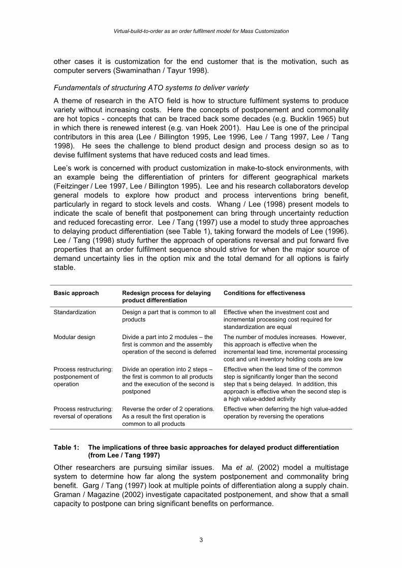
A theme of research in the ATO field is how to structure fulfilment systems to produce variety without increasing costs. Here the concepts of postponement and commonality are hot topics - concepts that can be traced back some decades (e.g. Bucklin 1965) but in which there is renewed interest (e.g. van Hoek 2001). Hau Lee is one of the principal contributors in this area (Lee / Billington 1995, Lee 1996, Lee / Tang 1997, Lee / Tang 1998). He sees the challenge to blend product design and process design so as to devise fulfilment systems that have reduced costs and lead times.
Lee’s work is concerned with product customization in make-to-stock environments, with an example being the differentiation of printers for different geographical markets (Feitzinger / Lee 1997, Lee / Billington 1995). Lee and his research collaborators develop general models to explore how product and process interventions bring benefit, particularly in regard to stock levels and costs. Whang / Lee (1998) present models to indicate the scale of benefit that postponement can bring through uncertainty reduction and reduced forecasting error. Lee / Tang (1997) use a model to study three approaches to delaying product differentiation (see Table 1), taking forward the models of Lee (1996). Lee / Tang (1998) study further the approach of operations reversal and put forward five properties that an order fulfilment sequence should strive for when the major source of demand uncertainty lies in the option mix and the total demand for all options is fairly stable.
Basic approach Redesign process for delaying
product differentiation Conditions for effectiveness
Standardization Design a part that is common to all products
Effective when the investment cost and incremental processing cost required for standardization are equal
Modular design Divide a part into 2 modules – the first is common and the assembly operation of the second is deferred
The number of modules increases. However, this approach is effective when the incremental lead time, incremental processing cost and unit inventory holding costs are low
Process restructuring: postponement of operation
Divide an operation into 2 steps – the first is common to all products and the execution of the second is postponed
Effective when the lead time of the common step is significantly longer than the second step that s being delayed. In addition, this approach is effective when the second step is a high value-added activity
Process restructuring: reversal of operations
Reverse the order of 2 operations. As a result the first operation is common to all products
Effective when deferring the high value-added operation by reversing the operations
Table 1: The implications of three basic approaches for delayed product differentiation (from Lee / Tang 1997)
Other researchers are pursuing similar issues. Ma et al. (2002) model a multistage system to determine how far along the system postponement and commonality bring benefit. Garg / Tang (1997) look at multiple points of differentiation along a supply chain. Graman / Magazine (2002) investigate capacitated postponement, and show that a small capacity to postpone can bring significant benefits on performance.
Brabazon and MacCarthy
4
Swaminathan / Tayur (1998, 1999) are the most comprehensive in applying postponement and commonality ideas to a mass customization problem. In their first study they develop a computational model to tackle a problem in which a producer offers a broad product range but in each time period orders are received for a fraction of variants only. They compare a vanilla box strategy (in which sub-sets of components are pre-assembled into a number of vanilla boxes, exploiting the inherent commonality in the product family) against MTS and ATO strategies and find the vanilla box approach can be superior significantly. In exploring their model, they show how factors including capacity constraints, demand correlation, number of vanilla box types and breadth of product range alter the performance of each strategy.
In the discussion of their model they suggest several approaches that a producer may find to be cost effective:
• product line specific vanilla boxes; where a sub-group of products are built from a specific vanilla box, rather than from any suitable vanilla box.
• substitution; three forms of substitution are available – component, vanilla box and product. Cost is incurred due to the substituted item having a higher cost than the required item.
• redundancy of components: where a vanilla box (or product) has un-required component(s).
In their second study, Swaminathan / Tayur (1999) go on to develop computational models that take account of assembly precedence constraints, in particular the feasibility of a vanilla box in terms of whether it can be assembled. They extend an existing three-way categorisation of components in regard to their effect on assembly:
• invariant components: that do not change their identity across the product line;
• pseudo variant components: that are different in products but do not change anything in the assembly sequence since they are all placed at the same position in the assembly sequence; and
• variant components: that are different in products and also could occur at different positions in the assembly sequence
Swaminathan / Tayur (1999) divide pseudo into two sub-categories – simple pseudo and complex pseudo – to recognize that the challenge (and cost) of making a component a pseudo variant can be negligible or significant. Their model incorporates fixed design costs that are incurred to enable delayed differentiation during final assembly and takes into account operational costs due to shortages, holding of inventory and overtime, and it allows them to investigate the differences between which component type is used for implementing variety. They find that providing more options in a smaller number of features and sequencing them based on the demand variance may be beneficial to the manufacturer both in terms of design and operations cost. They also find that set-up plays an important role in the determination of the optimal configurations, assembly sequence and costs incurred.
Assembly line design
Bradley / Blossom (2001) estimate the change in cost and the improvement in delivery lead time that would be achieved by an assembly process if it were to accept a higher proportion of customer orders. The study is focused on the automotive sector and the
Virtual-build-to-order as an order fulfilment model for Mass Customization
5
order fulfillment process under consideration closely resembles a VBTO system. The study does not look at how customer orders are matched to vehicles in the pipeline, but recognizes this is an area that needs attention. Their supposition is that flexibility can be increased in the assembly line by adding production capacity (people or equipment) so that a fluctuating mix of products can be produced. Thus the products made on the assembly line can be those that the customers want, when they want them, rather than units selected for attainment of maximum efficiency. By simulating a generic automotive system they estimate, in the worst case, cost would rise by around 0.017% at a level of 70% make-to-order (a significant reason being that direct labour accounts for only 6% of costs typically) and delivery lead times would reduced by around 70%.
Bukchin et al.. (2002) develop a heuristic for designing assembly lines for mixed model operations. They assume the model-mix is determined ahead of time and stable (say for a year ahead) but the sequence of launching products to the line must be determined by actual short range demand patterns and customer orders. Their approach assumes a model mix for which the combined workload is balanced for the duration of the entire shift and not on the basis of station cycle times (as was the case for single model assembly). The task allocation to stations must not violate precedence relations and they assume that for a family of similar models there are no contradictions between task precedence across different models. Compared to traditional lines, it is assumed worker competence allows tasks to be distributed more freely along the line, meaning fewer tasks are tied to a specific workstation, so creating options for assembly line design.
2.1.2. Variety in MTO
Manufacturers of complex goods such as machine tools have been facing the challenges of increased product diversity and shortening of delivery lead times. The requested delivery lead time is often less than the sum of purchasing, fabrication and assembly lead times. As a consequence such companies have been evolving their order fulfillment processes.
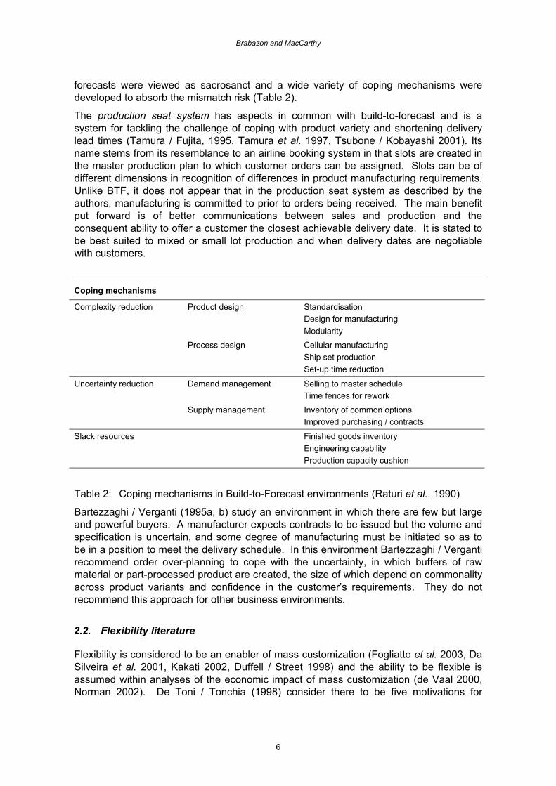
In their study of three heavy manufacturing firms Raturi et al.. (1990) describe the coping strategies they observe being used in response to shortening delivery schedules and increasing variety. They describe how firms have implemented a build-to-forecast (BTF) schedule, in which they forecast end-product mix, creating a master schedule of end-products and then releasing production orders before specific customer orders are received. In BTF there is no stopping point in the production process and buffer inventories are avoided. Customer orders arrive throughout the production process and are matched to items in any state of production that will meet the due date. Customer orders rarely match the end products being built hence orders are fulfilled by:
• changing products early in the process if the basic model is an appropriate one and the production plan can be altered to accommodate the actual order;
• reconfiguring an end product, with features removed and replaced as required. On occasion the changes are so extensive that a loss may be incurred.
Raturi et al.. consider there to be two approaches to coping in the BTF environment. One is to reduce the problem’s severity – in effect to reduce the gamble by somehow limiting the occurrence of a mismatch between customer orders and production units in progress. The other is to find better scheduling practices that would optimise the process of matching partially completed units to customer orders. However, in the firms studied the problem was rarely seen as a scheduling or forecasting issue. Instead the schedule and
Brabazon and MacCarthy
6
forecasts were viewed as sacrosanct and a wide variety of coping mechanisms were developed to absorb the mismatch risk (Table 2).
The production seat system has aspects in common with build-to-forecast and is a system for tackling the challenge of coping with product variety and shortening delivery lead times (Tamura / Fujita, 1995, Tamura et al. 1997, Tsubone / Kobayashi 2001). Its name stems from its resemblance to an airline booking system in that slots are created in the master production plan to which customer orders can be assigned. Slots can be of different dimensions in recognition of differences in product manufacturing requirements. Unlike BTF, it does not appear that in the production seat system as described by the authors, manufacturing is committed to prior to orders being received. The main benefit put forward is of better communications between sales and production and the consequent ability to offer a customer the closest achievable delivery date. It is stated to be best suited to mixed or small lot production and when delivery dates are negotiable with customers.
Coping mechanisms
Complexity reduction Product design Standardisation Design for manufacturing Modularity
Process design Cellular manufacturing Ship set production Set-up time reduction
Uncertainty reduction Demand management Selling to master schedule Time fences for rework
Supply management Inventory of common options Improved purchasing / contracts
Slack resources Finished goods inventory Engineering capability Production capacity cushion
Table 2: Coping mechanisms in Build-to-Forecast environments (Raturi et al.. 1990)
Bartezzaghi / Verganti (1995a, b) study an environment in which there are few but large and powerful buyers. A manufacturer expects contracts to be issued but the volume and specification is uncertain, and some degree of manufacturing must be initiated so as to be in a position to meet the delivery schedule. In this environment Bartezzaghi / Verganti recommend order over-planning to cope with the uncertainty, in which buffers of raw material or part-processed product are created, the size of which depend on commonality across product variants and confidence in the customer’s requirements. They do not recommend this approach for other business environments.
2.2. Flexibility literature
Flexibility is considered to be an enabler of mass customization (Fogliatto et al. 2003, Da Silveira et al. 2001, Kakati 2002, Duffell / Street 1998) and the ability to be flexible is assumed within analyses of the economic impact of mass customization (de Vaal 2000, Norman 2002). De Toni / Tonchia (1998) consider there to be five motivations for
Virtual-build-to-order as an order fulfilment model for Mass Customization
7
flexibility: variability of demand (random or seasonal); shorter life-cycles of the products and technologies; wider range of products; increased customization; and shorter delivery times.
The breadth of the topic is vast and so wide ranging that even within the large volume of literature there is little that addresses mass customization directly. At one end flexibility is addressed as a concept, at the other it is examined in the context of a specific situation. The scale of concern ranges from the flexibility of a sector down to the flexibility of a machine or fixtures and the concept also has a temporal property – flexibility over a short or long time horizon. Relevant literature is summarised under four headings: categories of flexibility; measurement of flexibility; enablers of flexibility and investment in flexibility.
2.2.1. Categories of flexibility
Interest in manufacturing flexibility grew in the 1980’s (e.g. Slack 1987, Gerwin 1989) and a number of taxonomies have been developed and augmented to the point where 15 types of manufacturing flexibility have been identified (Table 3). The categories in Table 3 would appear to be appropriate and sufficient for any, but a problem with defining flexibility is that context has a bearing. For example, to investigate the automotive sector, Koste / Malhotra (2000) judged the five flexibility dimensions of relevance were: machine flexibility, labour flexibility, mix flexibility, new product flexibility, and modification flexibility. Four of these map well onto the dimensions of Vokurka / O'Leary-Kelly (2000) but modification flexibility, which is concerned with the producer’s ability to accommodate customer selected options, is more context-specific than any dimension in Table 3.
Dimension Description
Machine range of operations that a piece of equipment can perform without incurring a major setup
Material handling
capabilities of a material handling process to move different parts throughout the manufacturing system
Operations number of alternative processes or ways in which a part can be produced within the system
Automation extent to which flexibility is housed in the automation computerization of manufacturing technologies
Labor range of tasks that an operator can perform within the manufacturing system
Process number of different parts that can be produced without incurring a major setup Routing number of alternative paths a part can take through the system in order to be completed Product time it takes to add or substitute new parts into the system New design speed at which products can be designed and introduced into the system
Delivery ability of the system to respond to changes in delivery requests Volume range of output levels that a firm can economically produce products Expansion ease at which capacity may be added to the system Program length of time the system can operate unattended Production range of products the system can produce without adding new equipment
Market ability of the manufacturing system to adapt to changes in the market environment
Table 3: Definitions of flexibility dimensions (Vokurka / O'Leary-Kelly 2000)
Brabazon and MacCarthy
8
A great number of flexibility dimensions can be found in the literature (of which an excellent review is provided by De Toni / Tonchia, 1998) and some make the linkage between customization and flexibility more overt than others. For example Parthasarthy / Sethi (1992) have two dimensions: speed flexibility which refers to the rapidity with which a production system can deliver finished products when required, change its volume rate and modify its product mix; and scope flexibility which refers to the breadth of products, including the degree of customization that a production system offers.
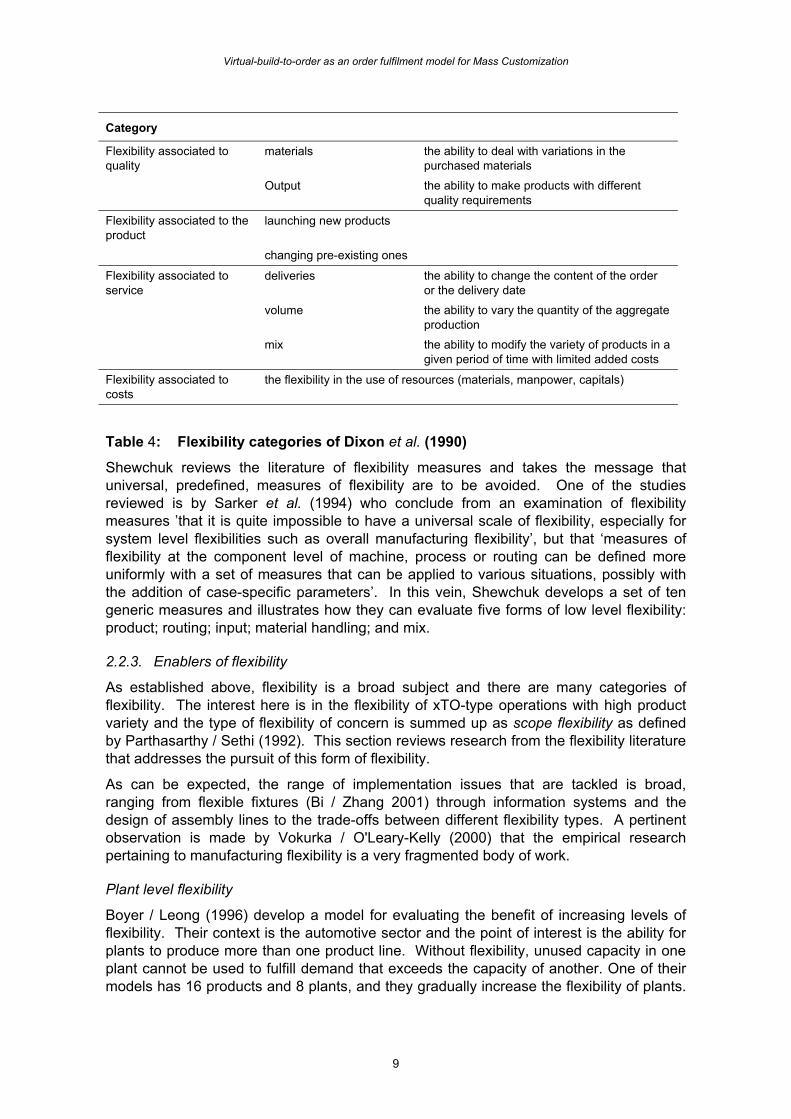
Two other aspects of flexibility are of relevance to the VBTO strategy. The first is that as well as flexibility being viewed as an enabler of customization, customization can be interpreted as a further category of flexibility. This perspective becomes clearer when reviewing a classification such as that of Dixon et al. (1990) in Table 4 which includes a category for being able to make products with different quality requirements, which is almost identical to one of ten customizable product attributes described in MacCarthy / Brabazon (2003).
The second aspect is the distinction made by some, such as Brandolese (1990) between the act of being flexible from the capability that enables flexibility. As reported in De Toni / Tonchia (1998), Brandolese separates flexibility - the software or managerial feature of the manufacturing system as a whole - from versatility which is the intrinsic or hardware feature of the manufacturing system that facilitates flexibility. In the context of responsiveness of which flexibility is a component, Kritchanchai / MacCarthy (1999) make a similar disictinction.
2.2.2. Measurement of flexibility
Just as the definitions of flexibility are found to be both universal but then insufficient for specific contexts, a similar story is found for measures of flexibility. Shewchuk (1999) notes two problems with developing flexibility measures:
“The first is that the difficulty of defining flexibility has resulted in definitions which are incomplete and/or ambiguous, measures which do not entirely match the corresponding definitions, and identical terms which are defined and/or measured differently. The second is that because every manufacturing enterprise, environment, and business strategy is unique in some manner, there is no guarantee that the assumptions upon which a given flexibility type or measure is based will be valid for a particular application.”
Category
Virtual-build-to-order as an order fulfilment model for Mass Customization
9
Category
Flexibility associated to quality
materials the ability to deal with variations in the purchased materials
Output the ability to make products with different quality requirements
Flexibility associated to the product
launching new products
changing pre-existing ones
Flexibility associated to service
deliveries the ability to change the content of the order or the delivery date
volume the ability to vary the quantity of the aggregate production
mix the ability to modify the variety of products in a given period of time with limited added costs
Flexibility associated to costs
the flexibility in the use of resources (materials, manpower, capitals)
Table 4: Flexibility categories of Dixon et al. (1990)
Shewchuk reviews the literature of flexibility measures and takes the message that universal, predefined, measures of flexibility are to be avoided. One of the studies reviewed is by Sarker et al. (1994) who conclude from an examination of flexibility measures ’that it is quite impossible to have a universal scale of flexibility, especially for system level flexibilities such as overall manufacturing flexibility’, but that ‘measures of flexibility at the component level of machine, process or routing can be defined more uniformly with a set of measures that can be applied to various situations, possibly with the addition of case-specific parameters’. In this vein, Shewchuk develops a set of ten generic measures and illustrates how they can evaluate five forms of low level flexibility: product; routing; input; material handling; and mix.
2.2.3. Enablers of flexibility
As established above, flexibility is a broad subject and there are many categories of flexibility. The interest here is in the flexibility of xTO-type operations with high product variety and the type of flexibility of concern is summed up as scope flexibility as defined by Parthasarthy / Sethi (1992). This section reviews research from the flexibility literature that addresses the pursuit of this form of flexibility.
As can be expected, the range of implementation issues that are tackled is broad, ranging from flexible fixtures (Bi / Zhang 2001) through information systems and the design of assembly lines to the trade-offs between different flexibility types. A pertinent observation is made by Vokurka / O'Leary-Kelly (2000) that the empirical research pertaining to manufacturing flexibility is a very fragmented body of work.
Plant level flexibility
Boyer / Leong (1996) develop a model for evaluating the benefit of increasing levels of flexibility. Their context is the automotive sector and the point of interest is the ability for plants to produce more than one product line. Without flexibility, unused capacity in one plant cannot be used to fulfill demand that exceeds the capacity of another. One of their models has 16 products and 8 plants, and they gradually increase the flexibility of plants.
Brabazon and MacCarthy
10
Perfect flexibility (no loss of throughput) and three levels of throughput loss are assessed. They find that opening up a fraction of the feasible cross-links between products and plants brings substantial gains in overall performance, even with a throughput loss of 20%.
Supply chain flexibility
To counter supply chain effects, the Quantity Flexibility (QF) contract has become popular (Tsay / Lovejoy 1999). It attaches a degree of commitment to the forecasts by installing constraints on the buyer’s ability to revise them over time. The extent of revision flexibility is defined in percentages that vary as a function of the number of periods away from delivery. The QF contract formalizes the reality that a single lead time alone is an inadequate representation of many supply relationships, as evinced by the ability of buyers to negotiate quantity changes even within quoted lead times. The model indicates that inventory is a consequence of disparities in flexibility. In particular, inventory is the cost incurred in overcoming the inflexibility of a supplier to meet a customer’s desire for flexible response and they coin the term flexibility amplification. All else being equal, increasing a supply chain participant’s input flexibility reduces its costs. And all else equal, promising more output flexibility comes at the expense of greater inventory costs. In addition, QF contracts can dampen the transmission of order variability throughout the chain, thus potentially retarding the well-known “bullwhip effect”. Tsay / Lovejoy provide a methodology for computing a materials manager’s “willingness-to-pay” for flexibility from an external vendor, which has certain properties. These include the notions that flexibility increases in value as the market environment becomes more volatile, and that flexibility observes a principle of diminishing returns. The buyer always prefers more flexibility, but should be careful to make the appropriate cost-benefit assessment in negotiating the contract.
2.2.4. Investment in flexibility
Research into the justification for investing in flexibility approaches the problem from an operations perspective (e.g. Fine / Freund 1990, Chang / Tsou 1993, Van Mieghem 1994) and another is from the viewpoint of business competition (e.g. De Vaal 2000, Norman 2002). One of the issues is over or under investment in flexibility as considered by Norman (2002) which brings out the point that flexibility has two components – the infrastructure that enables flexibility, and the use of this capability as and when required.
2.3. Customer differences literature
Differences across customers are, of course, the prime reason for the growth in product variety. However, customer differences can be expected to create other forms of ‘service’ variety within the order fulfillment system, such as variety in lead time and price.
Price and lead-time are interrelated. Price is connected to value (e.g. Meredith et al. 1994) and it is well understood that value tends to decay over time (e.g. Lindsay / Feigenbaum 1984). However, the rate of decay is not uniform across customer groups and for some customers, delivery earlier than an agreed date is undesirable.
Methodologies for exploiting customer differences are now emerging under the banner of yield management (also known as revenue management) and its proponents see many opportunities for exploiting its principles (Marmorstein et al. 2003) but the research in the xTO sector is scarce. Tang / Tang (2002) study time-based policies on pricing and lead-
Virtual-build-to-order as an order fulfilment model for Mass Customization
11
time for a build-to-order and direct sales manufacturer of products whose value is decreasing rapidly, such as is the case with high technology components. Although Chen (2001) is not focusing on high variety systems, his work is relevant. He proposes customers be given the opportunity to select from a menu of price and lead time combinations, with greater price discounts on offer for longer delivery times. By reducing the proportion of customers who demand immediate fulfillment, his model shows how safety stock/inventory along a supply system can be reduced hence costs are reduced and margins maintained.
What is lacking in the literature is an examination of how tolerant customers are to compromise in the product’s specification, and how this form of compromise interacts with price and lead-time. Products can have many customizable features and it is possible there will be customers for whom control of all features is preferred, but for others it could be the case that at least one of the features is of no great importance or is less important than, for example, delivery date.
2.4. Discussion
Insufficient time for operations and limited capacity are key hurdles as product variety rises especially in to-order environments. The Inability to complete the product in the time available forces speculation. In a low variety environment, only volume is speculated, but in a high variety environment both variety and volume need to be speculated on.
One of the main themes in the literature is that to cope in high variety to-order environments requires more than clever scheduling. Instead it is necessary to design the product and process to create flexibility.
The demands of high variety to-order environments is leading to the standard assumptions and models of order fulfilment systems being revisited. Bradley / Blossom (2001) provide such an example in their proposal that accepting a small increases in assembly operations cost can bring greater benefit in terms of customer service.
Imaginative approaches to fulfilling customers are being proposed, such as the method of substituting components or the non-removal of redundant components. Although they may be imperfect solutions, their adoption at the right moment may allow overall system performance to be improved. Here we propose a list of approaches:
• Specification substitution: the customer receives a superior option (as judged by the producer) to their target option, but they pay only for the target option;
• Specification redundancy: the customer receives an additional feature to their target specification but they do not pay for it (and they may not be aware of the additional feature);
• Specification reconfiguration: the product is amended to be exactly as the customer has ordered;
• Specification compromise: the customer receives a different option to their target option, and they pay for the option they received, perhaps with a discount as an incentive.
These forms of specification fulfillment are not always possible. Redundancy is open only if the product has more features than the customer is interested in. Substitution is
Brabazon and MacCarthy
12
not valid for all customizable attributes, e.g. in dimensional customization of garments you cannot substitute a shorter leg. In all methods the enterprise loses margin, either through reducing the price or incurring costs. The opportunity for each depends on the differences between the specification of the product from the customer’s specification, and on the point along the pipeline it has reached (e.g. it may not yet have had a redundant feature added).
The ability to choose between these types of specification fulfilment is a form of flexibility, but not one that is found in the flexibility literature.
3. Virtual-build-to-order (VBTO) system
This section of the paper describes the VBTO system in detail. VBTO has been conceived of being suited to market environments where there is diversity among customers in terms of demand for product variety and order fulfilment, particularly in regard to lead time. In regard to product specification, there may be customers with firm preferences across all aspects of the product’s specification, and other customers who are committed to few if any features of the specification.
Satisfying this range of customer types is demanding, particularly when the process lead time is greater than some (or all) customers are prepared to wait. The order fulfilment system devised for the computer servers (Swaminathan / Tayur 1998, 1999) uses a buffer of semi-finished inventory to cope with the uncertainties in customer demand. Several sectors, most notably the automotive and aerospace, are keen on the principles of lean manufacture, an objective of which is to have continuous processes with zero / minimal buffers. Furthermore, the competitive market place translates into the need for manufacturing facilities to be highly utilised. Nevertheless, these sectors are posed also with the challenge of increasing product variety. In the medium term (perhaps up to a year or so) the variety envelope can be constant, but in the short term the variety through manufacture must be shaped by customer orders (Bukchin et al. 2002).
Given their reluctance to tolerate inventory, these enterprises need other approaches to cope with the complexity of the business environment and market place. Rather than use inventory they need to develop appropriate process flexibilities, such as the ability to tolerate greater sequence variation through assembly flow lines (e.g. Boyer & Leong 1996, Bradley & Blossom 2001). It is for circumstances just as these that the VBTO system is intended.
A fundamental capability for a VBTO system is the ability to search the order fulfilment pipeline on behalf of a customer. The pipeline is the full set of unsold finished stock and unallocated production orders. A second capability that is desirable is the ability to reconfigure a product in the pipeline – i.e. change its specification to reduce or remove differences between it and the customer’s preferred specification. In a VBTO system, when a customer arrives, the producer can search the pipeline, which constitutes finished stock, products in production and products slated for production. If no exact match is available a suitable product can be reconfigured. Some reconfigurations may be possible once the product has left the factory, which is equivalent to form customization as defined by Alford et al. (2000). More extensive reconfigurations – labelled optional customization by Alford et al. - are likely to be more feasible the earlier the product is in the production plan.
Virtual-build-to-order as an order fulfilment model for Mass Customization
13
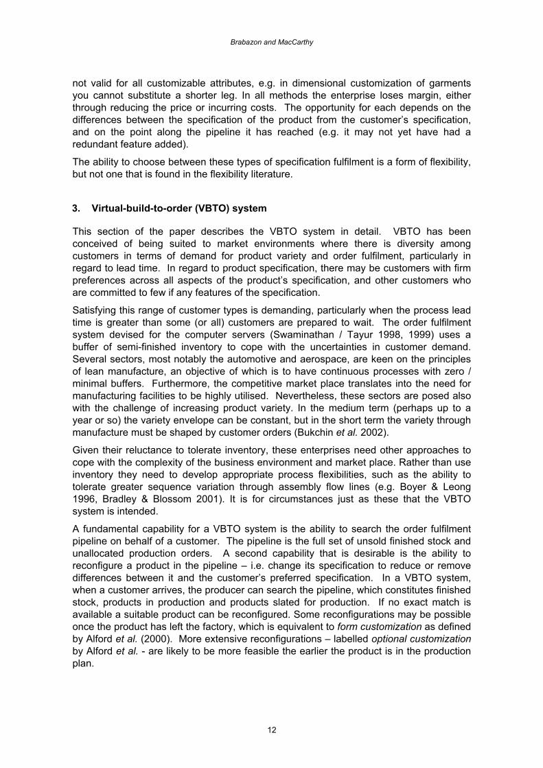
3.1. VBTO system structure
In a VBTO system the order fulfilment pipeline can be conceived of as a series of segments (Figure 1). The final segment is the stock held at each retailer (retailer stock) which may come via stock depots or direct from the factory segment. The finished stock and manufacturing segments make up the physical portion of the pipeline, in front of which is the virtual portion which itself is divided into several segments. The virtual segment of the pipeline is the production plan. The longer the production plan, the longer the virtual segment. The separate segments of the virtual portion represent the firmness and constraints on the production plan - as a product order moves from one segment to another on the virtual portion its specification becomes frozen (as described below). The orders in the final virtual segment are frozen and cannot be changed in terms of specification or sequence. The diagram shows three types of orders moving through the pipeline. Both customer assigned orders and retailer locked orders go directly to the retailer from the manufacturing segment and hence cannot be re-allocated. Hence only open orders reside in the stock depots.
2 3 4
Virtual portion Physical portion
Factory segment
Stock depots
Retailer stocks
Open order
Retailer locked order
Customer assigned order (locked)
Segment 1
Planning segment
Figure 1: Pipeline segments of a VBTO system
Interpreting the pipeline in terms of automotive manufacture, the factory segment is the assembly plant and the production plan is disseminated to suppliers who then prepare to feed components to the plant in the required sequence.
3.2. Operation of the pipeline
• Order initiation and specification: Retailers initiate and ‘own’ orders. When an order is created it has a full product specification. The product’s specification is progressively frozen as it moves closer to manufacture. There are constraints on who can alter the specification of an order. Locked orders, whether assigned to a customer or not can be changed by the locking retailer only. Unlocked orders can be altered by the owning retailer.
Brabazon and MacCarthy
14
• Order locking: When an order is created it is either an open order or a locked order. An order assigned to a customer is a locked order automatically, but a retailer can lock orders that are not assigned to customers (e.g. for display models). Once locked only the owning retailer can unlock an order. As an open order progresses through the virtual segment it can be locked by the owning retailer at any time.
• Order trading: Open orders can be traded. A retailer can search the physical and virtual portions of the pipeline for a vehicle that matches a customer’s specification. The system may require consent from the owning dealer before ownership is transferred, or it may permit unconsensed trading (Hawkins 2003).
• Order sequencing: The orders initiated by retailers are sequenced by a master scheduler who takes account of two forms of constraints:
− component capacity constraints due to supplier production limits;
− assembly constraints. To maintain a balanced production line at the assembly plant, restrictions might be placed on the sequence of products.
• Searching for a match: To find a product for a customer a retailer can search the pipeline. The physical segment is searched first, then the virtual segment.
3.3. Fulfilling customers
This section provides further details on how customers are fulfilled.
3.3.1. Fulfilment modes
Customers can be fulfilled by receiving a product from any segment of the physical or virtual portion of the pipeline. The customer can receive a product with an exact match to their requested specification from stock, from the pipeline or by having an order entered at the start of the pipeline (i.e. a Built-to-Order product). Items in the virtual portion of the pipeline can be amended so as to match the customer’s specification, but it may also be possible for stock items to be amended in small ways. The other forms of fulfilment described in section 2.4 can also be used: specification substitution; specification redundancy; and specification compromise.
3.3.2. Fulfilment performance
The overall objective is to satisfy customers at the lowest operational cost. In this form of system customer satisfaction is a construct of two factors: aversion to waiting and aversion to compromise. Of these two, aversion to waiting is perhaps the more straightforward to quantify (see below). In respect of a multi-attribute product, where some features appeal to a customer on functional grounds while others are hedonistic in nature, assessing the degree of compromise becomes complex.
3.3.3. Producer costs and operational constraints
The types of costs a producer can incur:
• finished stock holding;
• substituting higher grade options;
• redundant options in the product;
Virtual-build-to-order as an order fulfilment model for Mass Customization
15
• costs of reconfiguration.
The time to fulfil customers and the costs incurred by the producer depends on the control policies of the producer. If the producer uses all methods of fulfilment including substitution, redundancy and reconfiguration, and places no cost limit on these, customers would be fulfilled in the shortest possible time. As a producer places stiffer constraints on the method of fulfilment, either by rejecting them, placing cost limits on them or other constraint such as quantity flexibility limits that act to reduce the availability of products, the time to fulfil customers will increase.
3.4. Elaboration of key concepts
This section expands on three key concepts for the VBTO system: reconfiguration cost; quantity flexibility limits; and customer aversion to waiting.
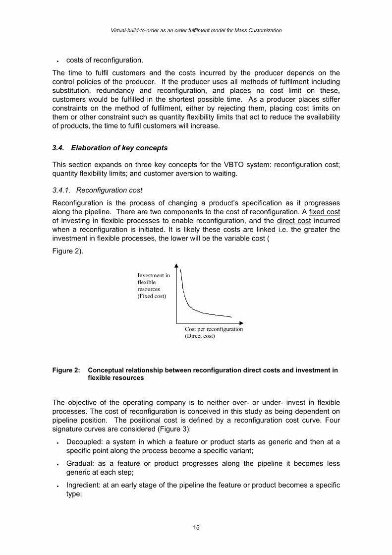
3.4.1. Reconfiguration cost
Reconfiguration is the process of changing a product’s specification as it progresses along the pipeline. There are two components to the cost of reconfiguration. A fixed cost of investing in flexible processes to enable reconfiguration, and the direct cost incurred when a reconfiguration is initiated. It is likely these costs are linked i.e. the greater the investment in flexible processes, the lower will be the variable cost (
Figure 2).
Cost per reconfiguration (Direct cost)
Investment in flexible resources (Fixed cost)
Figure 2: Conceptual relationship between reconfiguration direct costs and investment in
flexible resources
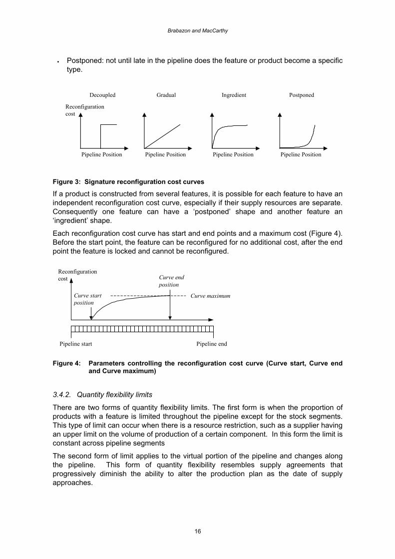
The objective of the operating company is to neither over- or under- invest in flexible processes. The cost of reconfiguration is conceived in this study as being dependent on pipeline position. The positional cost is defined by a reconfiguration cost curve. Four signature curves are considered (Figure 3):
• Decoupled: a system in which a feature or product starts as generic and then at a specific point along the process become a specific variant;
• Gradual: as a feature or product progresses along the pipeline it becomes less generic at each step;
• Ingredient: at an early stage of the pipeline the feature or product becomes a specific type;
Brabazon and MacCarthy
16
• Postponed: not until late in the pipeline does the feature or product become a specific type.
Pipeline Position
Reconfiguration cost
Pipeline Position Pipeline Position Pipeline Position
Decoupled Gradual Ingredient Postponed
Figure 3: Signature reconfiguration cost curves
If a product is constructed from several features, it is possible for each feature to have an independent reconfiguration cost curve, especially if their supply resources are separate. Consequently one feature can have a ‘postponed’ shape and another feature an ‘ingredient’ shape.
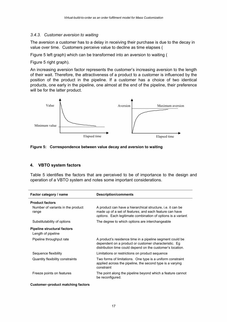
Each reconfiguration cost curve has start and end points and a maximum cost (Figure 4). Before the start point, the feature can be reconfigured for no additional cost, after the end point the feature is locked and cannot be reconfigured.
Pipeline start Pipeline end
Curve start position
Curve end position
Reconfiguration cost
Curve maximum
Figure 4: Parameters controlling the reconfiguration cost curve (Curve start, Curve end
and Curve maximum)
3.4.2. Quantity flexibility limits
There are two forms of quantity flexibility limits. The first form is when the proportion of products with a feature is limited throughout the pipeline except for the stock segments. This type of limit can occur when there is a resource restriction, such as a supplier having an upper limit on the volume of production of a certain component. In this form the limit is constant across pipeline segments
The second form of limit applies to the virtual portion of the pipeline and changes along the pipeline. This form of quantity flexibility resembles supply agreements that progressively diminish the ability to alter the production plan as the date of supply approaches.
Virtual-build-to-order as an order fulfilment model for Mass Customization
17
3.4.3. Customer aversion to waiting
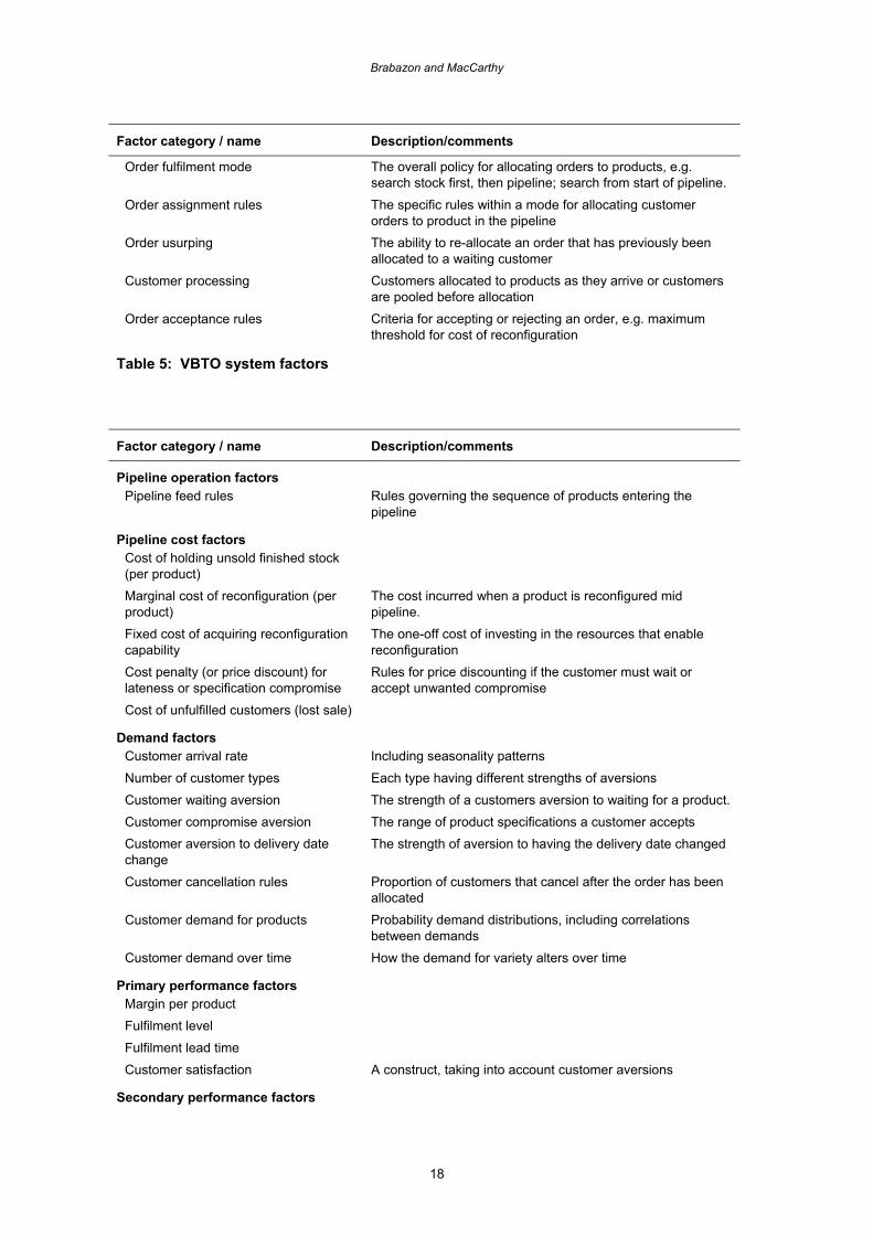
The aversion a customer has to a delay in receiving their purchase is due to the decay in value over time. Customers perceive value to decline as time elapses (
Figure 5 left graph) which can be transformed into an aversion to waiting (
Figure 5 right graph).
An increasing aversion factor represents the customer’s increasing aversion to the length of their wait. Therefore, the attractiveness of a product to a customer is influenced by the position of the product in the pipeline. If a customer has a choice of two identical products, one early in the pipeline, one almost at the end of the pipeline, their preference will be for the latter product.
Elapsed time
Value
Minimum value
Elapsed time
Aversion Maximum aversion
Figure 5: Correspondence between value decay and aversion to waiting
4. VBTO system factors
Table 5 identifies the factors that are perceived to be of importance to the design and operation of a VBTO system and notes some important considerations.
Factor category / name Description/comments
Product factors Number of variants in the product range
A product can have a hierarchical structure, i.e. it can be made up of a set of features, and each feature can have options. Each legitimate combination of options is a variant.
Substitutability of options The degree to which options are interchangeable
Pipeline structural factors Length of pipeline Pipeline throughput rate A product’s residence time in a pipeline segment could be
dependent on a product or customer characteristic. Eg distribution time could depend on the customer’s location.
Sequence flexibility Limitations or restrictions on product sequence Quantity flexibility constraints Two forms of limitations. One type is a uniform constraint
applied across the pipeline, the second type is a varying constraint
Freeze points on features The point along the pipeline beyond which a feature cannot be reconfigured.
Customer–product matching factors
Brabazon and MacCarthy
18
Factor category / name Description/comments
Order fulfilment mode The overall policy for allocating orders to products, e.g. search stock first, then pipeline; search from start of pipeline.
Order assignment rules The specific rules within a mode for allocating customer orders to product in the pipeline
Order usurping The ability to re-allocate an order that has previously been allocated to a waiting customer
Customer processing Customers allocated to products as they arrive or customers are pooled before allocation
Order acceptance rules Criteria for accepting or rejecting an order, e.g. maximum threshold for cost of reconfiguration
Table 5: VBTO system factors
Factor category / name Description/comments
Pipeline operation factors
Pipeline feed rules Rules governing the sequence of products entering the pipeline
Pipeline cost factors Cost of holding unsold finished stock (per product)
Marginal cost of reconfiguration (per product)
The cost incurred when a product is reconfigured mid pipeline.
Fixed cost of acquiring reconfiguration capability
The one-off cost of investing in the resources that enable reconfiguration
Cost penalty (or price discount) for lateness or specification compromise
Rules for price discounting if the customer must wait or accept unwanted compromise
Cost of unfulfilled customers (lost sale)
Demand factors Customer arrival rate Including seasonality patterns
Number of customer types Each type having different strengths of aversions Customer waiting aversion The strength of a customers aversion to waiting for a product. Customer compromise aversion The range of product specifications a customer accepts Customer aversion to delivery date change
The strength of aversion to having the delivery date changed
Customer cancellation rules Proportion of customers that cancel after the order has been allocated
Customer demand for products Probability demand distributions, including correlations between demands
Customer demand over time How the demand for variety alters over time
Primary performance factors Margin per product Fulfilment level
Fulfilment lead time Customer satisfaction A construct, taking into account customer aversions
Secondary performance factors
Virtual-build-to-order as an order fulfilment model for Mass Customization
19
Factor category / name Description/comments
Schedule disturbance Number of reconfigurations / substitutions
Number of reconfigurations incurring cost, and the number without incurring cost
Table 5: VBTO system factors (continued)
5. Simulation study of VBTO
In this and the following section of the paper the behaviour of the VBTO system is studied using simulation, to observe the effect of altering structural and control factors. This simulation study does not investigate all of the factors listed above. There is considerable scope for study of the VBTO system and this is the first stage of this process.
5.1. Description of the VBTO simulation model
5.1.1. Product structure
The product has a hierarchical structure of four independent features. The default in the study is for each feature to have four options, giving a total of 256 product variants, with all combinations being permitted. Other variety levels are investigated (from 2 options per feature up to 6 options per feature) and uneven distributions of variety across features are examined (e.g. as well as a 4,4,4,4 distribution of variety, cases such as 256,1,1,1 and 8,4,4,2 are tested).
5.1.2. Reconfiguration cost
In the simulation, reconfiguration cost is calculated as an additional cost, dependent on the position along the pipeline and the required change in the product specification. It is a cost that increases as a product progresses along the pipeline. The reconfiguration cost calculation for multi component products is given in [1].
RCMj = i=1Σn (δcij x fci) + 1 [1]
RCMj is the Reconfiguration cost multiplier for product in position j of the pipeline
δcij, the cost of reconfiguring feature i at position j of the pipeline
fci, the fraction of cost that feature i is of the total product
n is the number of features in the product
This equation generates a value greater than 1. For example, a value of 1.08 indicates that to reconfigure the product will add 8% to the cost compared to a non-reconfigured product. The equation returns a value of 1 if the product’s specification is an exact match to the customer’s specification.
Reconfiguration cost curve
The value of δc in equation [1] is defined by the feature’s reconfiguration cost curve. Each feature has an independent reconfiguration cost curve from the other features. In
Brabazon and MacCarthy
20
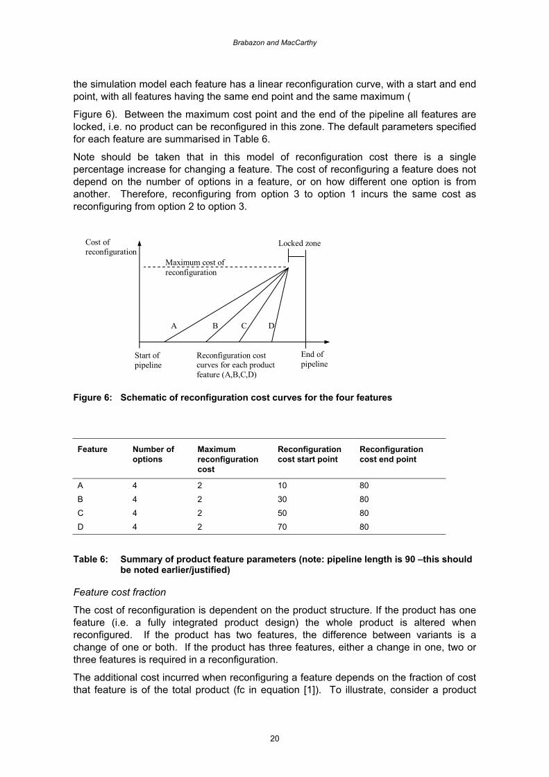
the simulation model each feature has a linear reconfiguration curve, with a start and end point, with all features having the same end point and the same maximum (
Figure 6). Between the maximum cost point and the end of the pipeline all features are locked, i.e. no product can be reconfigured in this zone. The default parameters specified for each feature are summarised in Table 6.
Note should be taken that in this model of reconfiguration cost there is a single percentage increase for changing a feature. The cost of reconfiguring a feature does not depend on the number of options in a feature, or on how different one option is from another. Therefore, reconfiguring from option 3 to option 1 incurs the same cost as reconfiguring from option 2 to option 3.
A B D C
Start of pipeline
End of pipeline
Locked zone
Maximum cost of reconfiguration
Cost of reconfiguration
Reconfiguration cost curves for each product feature (A,B,C,D)
Figure 6: Schematic of reconfiguration cost curves for the four features
Feature Number of
options Maximum reconfiguration cost
Reconfiguration cost start point
Reconfiguration cost end point
A 4 2 10 80
B 4 2 30 80 C 4 2 50 80 D 4 2 70 80
Table 6: Summary of product feature parameters (note: pipeline length is 90 –this should be noted earlier/justified)
Feature cost fraction
The cost of reconfiguration is dependent on the product structure. If the product has one feature (i.e. a fully integrated product design) the whole product is altered when reconfigured. If the product has two features, the difference between variants is a change of one or both. If the product has three features, either a change in one, two or three features is required in a reconfiguration.
The additional cost incurred when reconfiguring a feature depends on the fraction of cost that feature is of the total product (fc in equation [1]). To illustrate, consider a product
Virtual-build-to-order as an order fulfilment model for Mass Customization
21
comprising two features. If changing component A at position j of the pipeline adds 26% extra cost to feature A, and feature A is 66% of the cost of the product, and feature B, which is 33% of the product, costs 44% extra, then the additional cost of reconfiguring the product at position j is one of three:
(0.26 x 0.66) + 1 = 1.17 change feature A only
(0.44 x 0.33) + 1 = 1.15 change feature B only
(0.26 x 0.66 + 0.44 x 0.33) + 1 = 1.32 change features A and B
The default rule in the simulation is to make the fractional cost proportional to the variety carried by the feature. Table 7 gives examples to illustrate the rule. An alternative cost model is also investigated in the study (see later).
Variety per feature (A,B,C,D)
Fractional cost of each feature
A B C D
4,4,4,4 4/16 (i.e. 0.25) 4/16 4/16 4/16
32,2,2,2 32/38 2/38 2/32 2/32 128,2,1,1 128/130 2/130 0 0 256,1,1,1 256/256 (i.e. 1) 0 0 0
Table 7: Fractional cost of product features
5.1.3. Stock holding cost
The cost of holding stock is assumed to be low. The cost of holding a finished item in stock for one time period adds 1 x 10⁻⁷ % to the cost of a product (note: product rate and customer arrival rate are one per time period).
5.1.4. Pipeline factors
Pipeline length is 90 units.
5.1.5. Pipeline feed
In most of the analysis presented below the uniform random demand distribution is used for the feed into the pipeline, i.e. all product configurations have equal likelihood of being fed into the pipeline
5.1.6. Quantity flexibility constraints
Quantity flexibility limits are modelled by placing a constraint on the number of any one option being in the pipeline at one time. The effect of this is to inhibit the freedom to reconfigure products. For example, let’s say feature A has four options and a limit of 40% is placed on the proportion of products in the pipeline that can have an identical option for feature A. If a customer searches for a product with option 2 for feature A but no unassigned products have that specification, then only if there are fewer than 40% of products in the pipeline with option 2 already can another product be reconfigured to have option 2.
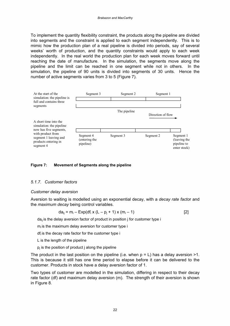
Brabazon and MacCarthy
22
To implement the quantity flexibility constraint, the products along the pipeline are divided into segments and the constraint is applied to each segment independently. This is to mimic how the production plan of a real pipeline is divided into periods, say of several weeks’ worth of production, and the quantity constraints would apply to each week independently. In the real world the production plan for each week moves forward until reaching the date of manufacture. In the simulation, the segments move along the pipeline and the limit can be reached in one segment while not in others. In the simulation, the pipeline of 90 units is divided into segments of 30 units. Hence the number of active segments varies from 3 to 5 (Figure 7).
Segment 1 Segment 2 Segment 3
Segment 1 (leaving the pipeline to enter stock)
Segment 2 Segment 3 Segment 4 (entering the pipeline)
At the start of the simulation: the pipeline is full and contains three segments
A short time into the simulation: the pipeline now has five segments, with product from segment 1 leaving and products entering in segment 4
The pipeline Direction of flow
Figure 7: Movement of Segments along the pipeline
5.1.7. Customer factors
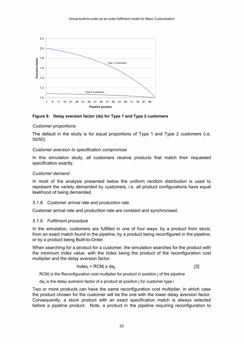
Customer delay aversion
Aversion to waiting is modelled using an exponential decay, with a decay rate factor and the maximum decay being control variables.
daij = mi – Exp(dfi x (L – pj + 1) x (mi – 1) [2]
daij is the delay aversion factor of product in position j for customer type i
mi is the maximum delay aversion for customer type i
dfi is the decay rate factor for the customer type i
L is the length of the pipeline
pj is the position of product j along the pipeline
The product in the last position on the pipeline (i.e. when p = L) has a delay aversion >1. This is because it still has one time period to elapse before it can be delivered to the customer. Products in stock have a delay aversion factor of 1.
Two types of customer are modelled in the simulation, differing in respect to their decay rate factor (df) and maximum delay aversion (m). The strength of their aversion is shown in Figure 8.
Virtual-build-to-order as an order fulfilment model for Mass Customization
23
1.0
1.2
1.4
1.6
1.8
2.0
2.2
1 6 11 16 21 26 31 36 41 46 51 56 61 66 71 76 81 86
Pipeline position
Ave
rsio
n fa
ctor
Type 1 Customers
Type 2 Customers
Figure 8: Delay aversion factor (da) for Type 1 and Type 2 customers
Customer proportions
The default in the study is for equal proportions of Type 1 and Type 2 customers (i.e. 50/50)
Customer aversion to specification compromise
In this simulation study, all customers receive products that match their requested specification exactly.
Customer demand
In most of the analysis presented below the uniform random distribution is used to represent the variety demanded by customers, i.e. all product configurations have equal likelihood of being demanded.
5.1.8. Customer arrival rate and production rate
Customer arrival rate and production rate are constant and synchronised.
5.1.9. Fulfilment procedure
In the simulation, customers are fulfilled in one of four ways: by a product from stock; from an exact match found in the pipeline; by a product being reconfigured in the pipeline; or by a product being Built-to-Order.
When searching for a product for a customer, the simulation searches for the product with the minimum index value, with the index being the product of the reconfiguration cost multiplier and the delay aversion factor:
Indexj = RCMj x daij [3]
RCMj is the Reconfiguration cost multiplier for product in position j of the pipeline
daij is the delay aversion factor of a product at position j for customer type i
Two or more products can have the same reconfiguration cost multiplier, in which case the product chosen for the customer will be the one with the lower delay aversion factor. Consequently, a stock product with an exact specification match is always selected before a pipeline product. Note, a product in the pipeline requiring reconfiguration to
Brabazon and MacCarthy
24
match a customer may have a lower index than a product with an exact specification match that is further upstream.
If no exact match can be found, and no product can be reconfigured, a request is sent to the start of the pipeline for a product to be Built-to-Order. In the simulation there are two situations in which a BTO request can be made. One is when quantity flexibility limits are in operation and the limits have been reached, and the second is when a limit is placed on the maximum reconfiguration cost that the producer will accept and there are no unallocated products that can be reconfigured to the customer’s specification for less than this limit.
When a request is made for a BTO product, it will wait at the start of the pipeline until it is permitted to enter the pipeline. In the conditions studied here, only the quantity flexibility limits can cause a BTO to wait – otherwise it enters immediately.
In all of the conditions studied, every customer is fulfilled and no customer cancels an order. As soon as a customer arrives, a product is sought and allocated to them and the search for a product is independent of the preceding or following customer.
When a product in the pipeline is allocated to a customer it remains in the pipeline, progressing to the end of the pipeline and unavailable to other customers. It disappears from the system when it reaches the end of the pipeline. Stock products that are allocated to customers are removed from stock immediately.
5.2. System conditions explored
The study reported here explores seven system conditions:
• ‘Basecase’: In this system a customer is fulfilled by an exact match from the pipeline or by a costless reconfiguration. This system resembles a producer who is not prepared to incur reconfiguration costs.
• Proportion of each customer type: the proportions of the two customer types are altered.
• Imposition of a limit on the reconfiguration cost: A new criteria is added to the system, which limits the reconfiguration cost incurred by the producer. The pipeline is searched for the product with the lowest index and then the reconfiguration cost is compared to the tolerated limit.
• Imposition of quantity flexibility limits: these limit the number of identical options in a segment of the pipeline. The pipeline is divided into segments of length 30, and the limits apply to each segment. Each feature has 4 options, and the effect on imposing throughput limits on all features, and then on only one feature is studied. Throughput limits of 8, 9, 10, 11 and 12 identical options per segment are imposed
• Alteration of the reconfiguration cost curves: three types of modification are made to the reconfiguration cost curve as illustrated in
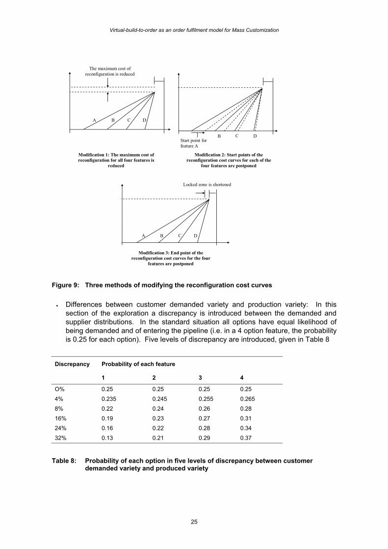
• Figure 9. In the first the maximum cost is lowered, at first by 10% and then a further 10%. In the second the start points are shifted in two stages. In the third the locked zone is reduced in two stages. Furthermore, all three modifications are combined to reveal their joint impact.
Virtual-build-to-order as an order fulfilment model for Mass Customization
25
Modification 2: Start points of the reconfiguration cost curves for each of the
four features are postponed
Modification 1: The maximum cost of reconfiguration for all four features is
reduced
B C D Start point for feature A
Locked zone is shortened
C D B A
Modification 3: End point of the reconfiguration cost curves for the four
features are postponed
A B D C
The maximum cost of reconfiguration is reduced
Figure 9: Three methods of modifying the reconfiguration cost curves
• Differences between customer demanded variety and production variety: In this section of the exploration a discrepancy is introduced between the demanded and supplier distributions. In the standard situation all options have equal likelihood of being demanded and of entering the pipeline (i.e. in a 4 option feature, the probability is 0.25 for each option). Five levels of discrepancy are introduced, given in Table 8
Discrepancy Probability of each feature
1 2 3 4
O% 0.25 0.25 0.25 0.25
4% 0.235 0.245 0.255 0.265 8% 0.22 0.24 0.26 0.28 16% 0.19 0.23 0.27 0.31 24% 0.16 0.22 0.28 0.34
32% 0.13 0.21 0.29 0.37
Table 8: Probability of each option in five levels of discrepancy between customer demanded variety and produced variety
Brabazon and MacCarthy
26
• Impact of production sequencing: Three forms of sequencing are investigated and compared to the random feed. The first is generic feed, in which a sequence of identical products are fed into the pipeline. Then two versions of cyclical sequencing are tested, one is cycling of feature A through its four options with the other three features being generic (i.e. always option 1), and the other is cycling through feature D options with the other three features being generic. Features A and D are compared as they are the most different in terms of their reconfiguration cost curves.
• Variety spread: the spread of variety across the product features is altered, from the situation of all features having equal variety (i.e. product structure of 4,4,4,4) to all variety being on one feature (e.g. 1,1,256,1). In all cases the variety is held constant. Several issues are investigated including the implication of altering the fractional cost factor (factor fc in equation [1]) .
• Customer aversion: the impact on order fulfilment metrics of different levels of customer aversion to waiting are investigated.
5.3. Simulation approach
A warm-up period of 500 customers has been allowed and the method of batch means, with a dead period between batches, used in the collection of data.
6. Results
6.1. Basecase
Although the two types of customers have different aversions to waiting, in the basecase system they have the same fulfilment performance. As variety increases the waiting time increases for both customers (
Figure 10). The proportion of customers fulfilled by reconfigured products follows the same pattern and again there is no difference between the two customer types.
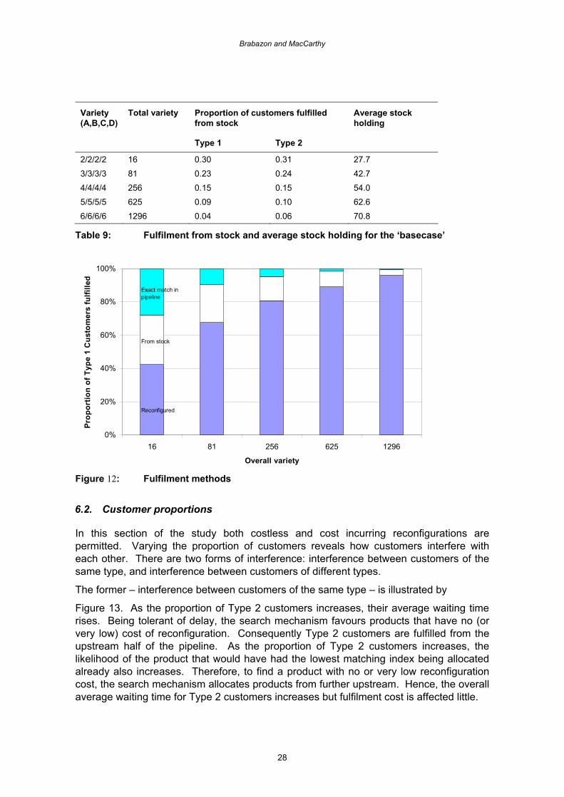
As product variety increases, the steady-state stock holding increases. In the simulation system there are always 90 unallocated products. This is because a) the customer arrival rate and production rate are equal, b) every customer is fulfilled, and c) the system starts with the pipeline full and stock empty. When a customer arrives, one product is allocated to them, and before the next customer arrives a new product enters the pipeline. At the lowest variety level studied (i.e. a product structure of 2,2,2,2), customers are fulfilled as follows: 40% by reconfigurations in the pipeline, 30% from stock and 30% by exact matches in the pipeline (Table 9: Fulfilment from stock and average stock holding for the ‘basecase’
). The average waiting time is just above 30% of the pipeline length. The consequence of this is that the majority of the 90 unallocated products are in the pipeline, with an average of ~28 of them in stock (Table 9). At the highest variety level studied (i.e. product structure 6,6,6,6) the dominant mode of fulfilment is by reconfigurations in the pipeline (~95%) which take place at the upstream end of the pipeline (indicated by the average waiting time being ~80% of the pipeline length). Consequently, products in the downstream of the pipeline at the start of the simulation move into stock and can reside
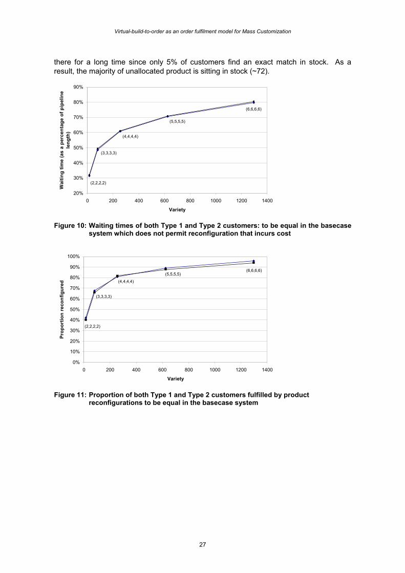
Virtual-build-to-order as an order fulfilment model for Mass Customization
27
there for a long time since only 5% of customers find an exact match in stock. As a result, the majority of unallocated product is sitting in stock (~72).
20%
30%
40%
50%
60%
70%
80%
90%
0 200 400 600 800 1000 1200 1400
Variety
Wai
ting
time
(as
a pe
rcen
tage
of p
ipel
ine
leng
th)
(2,2,2,2)
(3,3,3,3)
(4,4,4,4)
(5,5,5,5)
(6,6,6,6)
Figure 10: Waiting times of both Type 1 and Type 2 customers: to be equal in the basecase
system which does not permit reconfiguration that incurs cost
0%
10%
20%
30%
40%
50%
60%
70%
80%
90%
100%
0 200 400 600 800 1000 1200 1400
Variety
Prop
ortio
n re
conf
igur
ed
(2,2,2,2)
(3,3,3,3)
(4,4,4,4)
(5,5,5,5)(6,6,6,6)
Figure 11: Proportion of both Type 1 and Type 2 customers fulfilled by product
reconfigurations to be equal in the basecase system
Brabazon and MacCarthy
28
Variety (A,B,C,D)
Total variety Proportion of customers fulfilled from stock
Average stock holding
Type 1 Type 2
2/2/2/2 16 0.30 0.31 27.7 3/3/3/3 81 0.23 0.24 42.7
4/4/4/4 256 0.15 0.15 54.0 5/5/5/5 625 0.09 0.10 62.6 6/6/6/6 1296 0.04 0.06 70.8
Table 9: Fulfilment from stock and average stock holding for the ‘basecase’
0%
20%
40%
60%
80%
100%
16 81 256 625 1296
Overall variety
Prop
ortio
n of
Typ
e 1
Cus
tom
ers
fulfi
lled
Reconfigured
From stock
Exact match in pipeline
Figure 12: Fulfilment methods
6.2. Customer proportions
In this section of the study both costless and cost incurring reconfigurations are permitted. Varying the proportion of customers reveals how customers interfere with each other. There are two forms of interference: interference between customers of the same type, and interference between customers of different types.
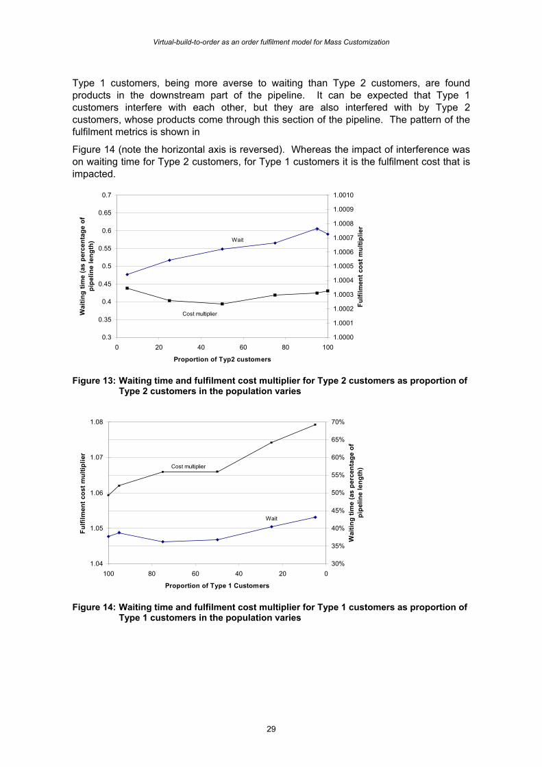
The former – interference between customers of the same type – is illustrated by
Figure 13. As the proportion of Type 2 customers increases, their average waiting time rises. Being tolerant of delay, the search mechanism favours products that have no (or very low) cost of reconfiguration. Consequently Type 2 customers are fulfilled from the upstream half of the pipeline. As the proportion of Type 2 customers increases, the likelihood of the product that would have had the lowest matching index being allocated already also increases. Therefore, to find a product with no or very low reconfiguration cost, the search mechanism allocates products from further upstream. Hence, the overall average waiting time for Type 2 customers increases but fulfilment cost is affected little.
Virtual-build-to-order as an order fulfilment model for Mass Customization
29
Type 1 customers, being more averse to waiting than Type 2 customers, are found products in the downstream part of the pipeline. It can be expected that Type 1 customers interfere with each other, but they are also interfered with by Type 2 customers, whose products come through this section of the pipeline. The pattern of the fulfilment metrics is shown in
Figure 14 (note the horizontal axis is reversed). Whereas the impact of interference was on waiting time for Type 2 customers, for Type 1 customers it is the fulfilment cost that is impacted.
0.3
0.35
0.4
0.45
0.5
0.55
0.6
0.65
0.7
0 20 40 60 80 100
Proportion of Typ2 customers
Wai
ting
time
(as
perc
enta
ge o
f pi
pelin
e le
ngth
)
1.0000
1.0001
1.0002
1.0003
1.0004
1.0005
1.0006
1.0007
1.0008
1.0009
1.0010
Fulfi
lmen
t cos
t mul
tiplie
r
Cost multiplier
Wait
Figure 13: Waiting time and fulfilment cost multiplier for Type 2 customers as proportion of
Type 2 customers in the population varies
30%
35%
40%
45%
50%
55%
60%
65%
70%
020406080100
Proportion of Type 1 Customers
Wai
ting
time
(as
perc
enta
ge o
f pi
pelin
e le
ngth
)
1.04
1.05
1.06
1.07
1.08
Fulfi
lmen
t cos
t mul
tiplie
r
Cost multiplier
Wait
Figure 14: Waiting time and fulfilment cost multiplier for Type 1 customers as proportion of
Type 1 customers in the population varies
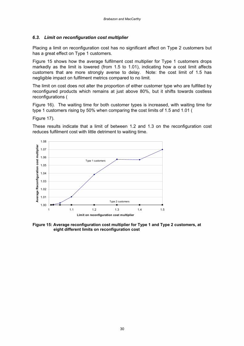
Brabazon and MacCarthy
30
6.3. Limit on reconfiguration cost multiplier
Placing a limit on reconfiguration cost has no significant affect on Type 2 customers but has a great effect on Type 1 customers.
Figure 15 shows how the average fulfilment cost multiplier for Type 1 customers drops markedly as the limit is lowered (from 1.5 to 1.01), indicating how a cost limit affects customers that are more strongly averse to delay. Note: the cost limit of 1.5 has negligible impact on fulfilment metrics compared to no limit.
The limit on cost does not alter the proportion of either customer type who are fulfilled by reconfigured products which remains at just above 80%, but it shifts towards costless reconfigurations (
Figure 16). The waiting time for both customer types is increased, with waiting time for type 1 customers rising by 50% when comparing the cost limits of 1.5 and 1.01 (
Figure 17).
These results indicate that a limit of between 1.2 and 1.3 on the reconfiguration cost reduces fulfilment cost with little detriment to waiting time.
1.00
1.01
1.02
1.03
1.04
1.05
1.06
1.07
1.08
1 1.1 1.2 1.3 1.4 1.5
Limit on reconfiguration cost multiplier
Ave
rage
Rec
onfig
urat
ion
cost
mul
tiplie
r
Type 1 customers
Type 2 customers
Figure 15: Average reconfiguration cost multiplier for Type 1 and Type 2 customers, at
eight different limits on reconfiguration cost
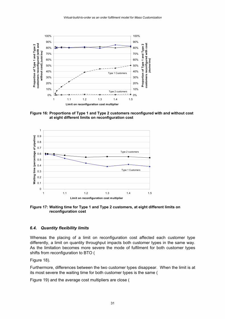
Virtual-build-to-order as an order fulfilment model for Mass Customization
31
0%
10%
20%
30%
40%
50%
60%
70%
80%
90%
100%
1 1.1 1.2 1.3 1.4 1.5
Limit on reconfiguration cost multiplier
Prop
ortio
n of
Typ
e 1
and
Type
2
cust
omer
s re
conf
igur
ed (w
ith a
nd
with
out c
ost)
[sol
id li
ne]
0%
10%
20%
30%
40%
50%
60%
70%
80%
90%
100%
Prop
ortio
n of
Typ
e 1
and
Type
2
cust
omer
s re
conf
igur
ed w
ith c
ost
[das
hed
line]
Type 2 customers
Type 1 Customers
Figure 16: Proportions of Type 1 and Type 2 customers reconfigured with and without cost
at eight different limits on reconfiguration cost
0
0.1
0.2
0.3
0.4
0.5
0.6
0.7
0.8
0.9
1
1 1.1 1.2 1.3 1.4 1.5
Limit on reconfiguration cost multiplier
Wai
ting
time
(per
cent
age
of p
ipel
ine)
Type 1 Customers
Type 2 customers
Figure 17: Waiting time for Type 1 and Type 2 customers, at eight different limits on
reconfiguration cost
6.4. Quantity flexibility limits
Whereas the placing of a limit on reconfiguration cost affected each customer type differently, a limit on quantity throughput impacts both customer types in the same way. As the limitation becomes more severe the mode of fulfilment for both customer types shifts from reconfiguration to BTO (
Figure 18).
Furthermore, differences between the two customer types disappear. When the limit is at its most severe the waiting time for both customer types is the same (
Figure 19) and the average cost multipliers are close (
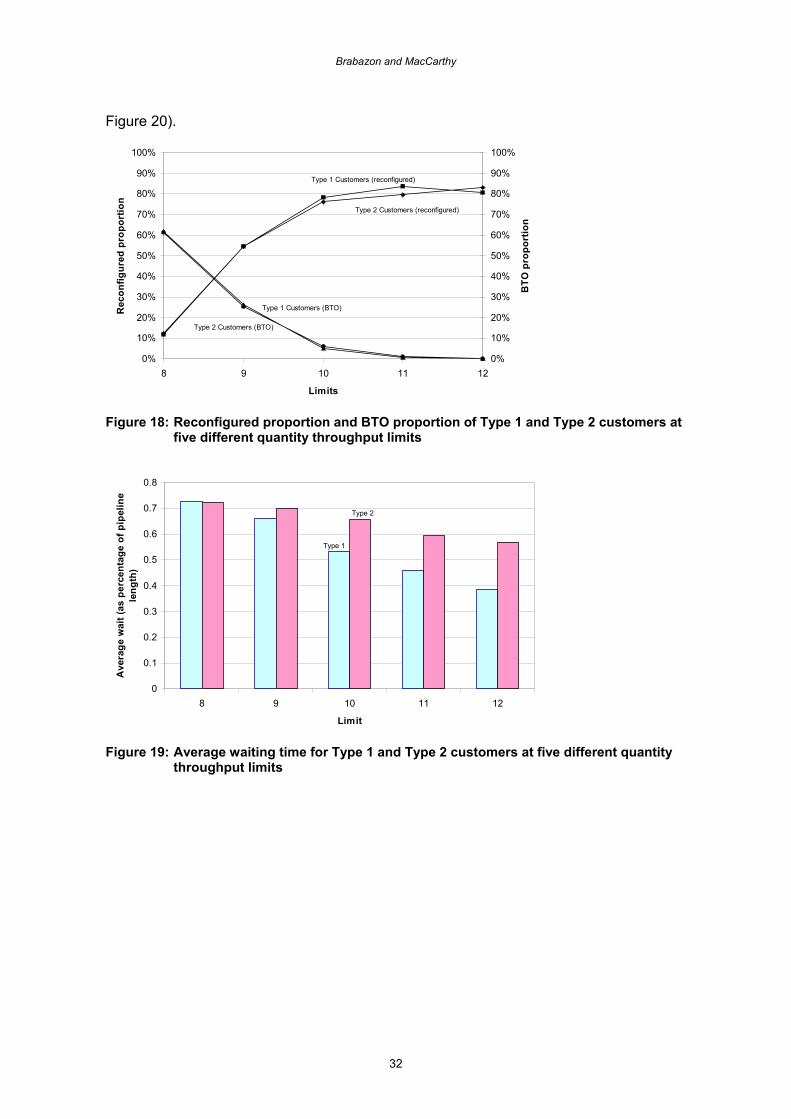
Brabazon and MacCarthy
32
Figure 20).
0%
10%
20%
30%
40%
50%
60%
70%
80%
90%
100%
8 9 10 11 12
Limits
Rec
onfig
ured
pro
port
ion
0%
10%
20%
30%
40%
50%
60%
70%
80%
90%
100%
BTO
pro
port
ion
Type 1 Customers (BTO)
Type 1 Customers (reconfigured)
Type 2 Customers (reconfigured)
Type 2 Customers (BTO)
Figure 18: Reconfigured proportion and BTO proportion of Type 1 and Type 2 customers at
five different quantity throughput limits
0
0.1
0.2
0.3
0.4
0.5
0.6
0.7
0.8
8 9 10 11 12
Limit
Ave
rage
wai
t (as
per
cent
age
of p
ipel
ine
leng
th)
Type 1
Type 2
Figure 19: Average waiting time for Type 1 and Type 2 customers at five different quantity
throughput limits
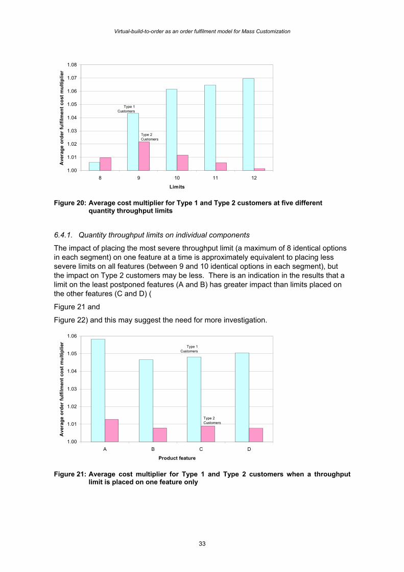
Virtual-build-to-order as an order fulfilment model for Mass Customization
33
1.00
1.01
1.02
1.03
1.04
1.05
1.06
1.07
1.08
8 9 10 11 12
Limits
Ave
rage
ord
er fu
lfilm
ent c
ost m
ultip
lier
Type 1 Customers
Type 2 Customers
Figure 20: Average cost multiplier for Type 1 and Type 2 customers at five different
quantity throughput limits
6.4.1. Quantity throughput limits on individual components
The impact of placing the most severe throughput limit (a maximum of 8 identical options in each segment) on one feature at a time is approximately equivalent to placing less severe limits on all features (between 9 and 10 identical options in each segment), but the impact on Type 2 customers may be less. There is an indication in the results that a limit on the least postponed features (A and B) has greater impact than limits placed on the other features (C and D) (
Figure 21 and
Figure 22) and this may suggest the need for more investigation.
1.00
1.01
1.02
1.03
1.04
1.05
1.06
A B C D
Product feature
Ave
rage
ord
er fu
lfilm
ent c
ost m
ultip
lier
Type 1 Customers
Type 2 Customers
Figure 21: Average cost multiplier for Type 1 and Type 2 customers when a throughput
limit is placed on one feature only
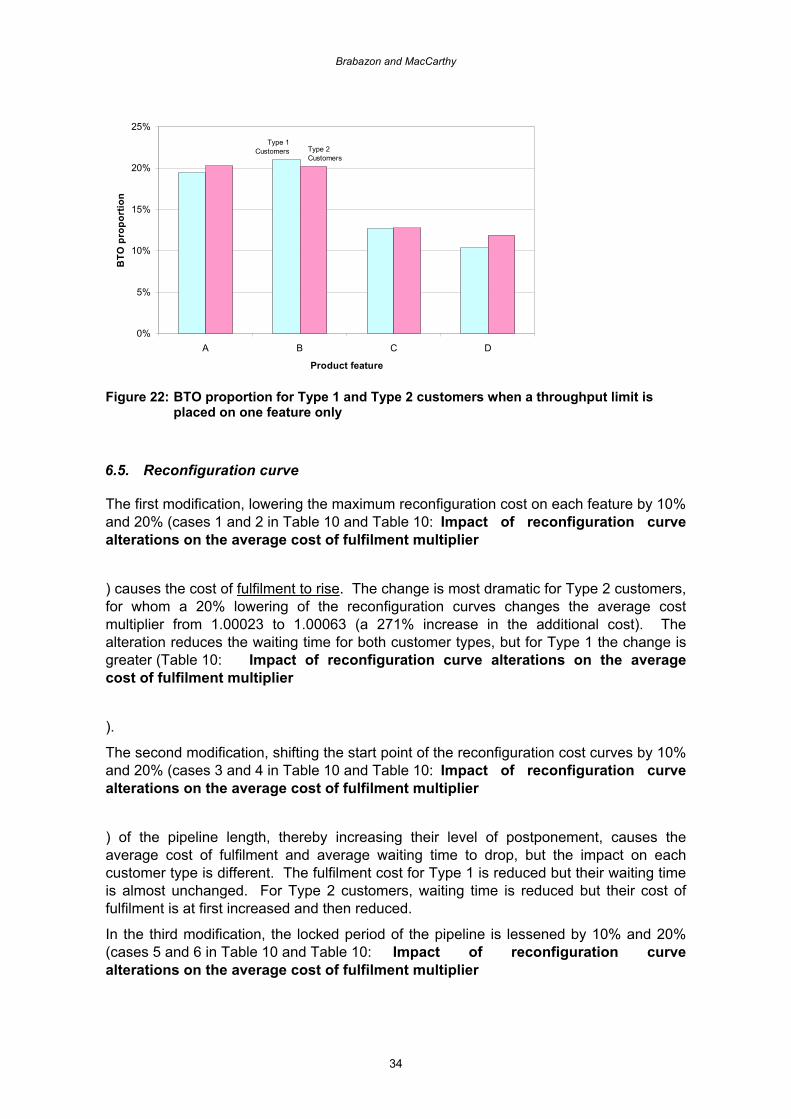
Brabazon and MacCarthy
34
0%
5%
10%
15%
20%
25%
A B C D
Product feature
BTO
pro
port
ion
Type 1 Customers Type 2
Customers
Figure 22: BTO proportion for Type 1 and Type 2 customers when a throughput limit is
placed on one feature only
6.5. Reconfiguration curve
The first modification, lowering the maximum reconfiguration cost on each feature by 10% and 20% (cases 1 and 2 in Table 10 and Table 10: Impact of reconfiguration curve alterations on the average cost of fulfilment multiplier
) causes the cost of fulfilment to rise. The change is most dramatic for Type 2 customers, for whom a 20% lowering of the reconfiguration curves changes the average cost multiplier from 1.00023 to 1.00063 (a 271% increase in the additional cost). The alteration reduces the waiting time for both customer types, but for Type 1 the change is greater (Table 10: Impact of reconfiguration curve alterations on the average cost of fulfilment multiplier
).
The second modification, shifting the start point of the reconfiguration cost curves by 10% and 20% (cases 3 and 4 in Table 10 and Table 10: Impact of reconfiguration curve alterations on the average cost of fulfilment multiplier
) of the pipeline length, thereby increasing their level of postponement, causes the average cost of fulfilment and average waiting time to drop, but the impact on each customer type is different. The fulfilment cost for Type 1 is reduced but their waiting time is almost unchanged. For Type 2 customers, waiting time is reduced but their cost of fulfilment is at first increased and then reduced.
In the third modification, the locked period of the pipeline is lessened by 10% and 20% (cases 5 and 6 in Table 10 and Table 10: Impact of reconfiguration curve alterations on the average cost of fulfilment multiplier
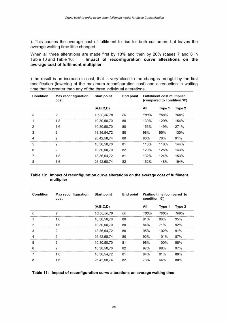
Virtual-build-to-order as an order fulfilment model for Mass Customization
35
). This causes the average cost of fulfilment to rise for both customers but leaves the average waiting time little changed.
When all three alterations are made first by 10% and then by 20% (cases 7 and 8 in Table 10 and Table 10: Impact of reconfiguration curve alterations on the average cost of fulfilment multiplier
) the result is an increase in cost, that is very close to the changes brought by the first modification (lowering of the maximum reconfiguration cost) and a reduction in waiting time that is greater than any of the three individual alterations. Condition Max reconfiguration
cost Start point End point Fulfillment cost multiplier
(compared to condition ‘0’)
(A,B,C,D) All Type 1 Type 2
0 2 10,30,50,70 80 100% 100% 100%
1 1.8 10,30,50,70 80 130% 129% 154%
2 1.6 10,30,50,70 80 153% 149% 271%
3 2 18,36,54,72 80 98% 95% 130%
4 2 26,42,58,74 80 80% 76% 91%
5 2 10,30,50,70 81 113% 110% 144% 6 2 10,30,50,70 82 129% 125% 143%
7 1.8 18,36,54,72 81 132% 124% 153% 8 1.6 26,42,58,74 82 152% 148% 194%
Table 10: Impact of reconfiguration curve alterations on the average cost of fulfilment multiplier
Condition Max reconfiguration cost
Start point End point Waiting time (compared to condition ‘0’)
(A,B,C,D) All Type 1 Type 2
0 2 10,30,50,70 80 100% 100% 100%
1 1.8 10,30,50,70 80 91% 86% 95%
2 1.6 10,30,50,70 80 84% 71% 92%
3 2 18,36,54,72 80 95% 102% 91% 4 2 26,42,58,74 80 92% 101% 87%
5 2 10,30,50,70 81 98% 100% 98% 6 2 10,30,50,70 82 97% 98% 97%
7 1.8 18,36,54,72 81 84% 81% 88%
8 1.6 26,42,58,74 82 73% 64% 80%
Table 11: Impact of reconfiguration curve alterations on average waiting time
Brabazon and MacCarthy
36
6.6. Mismatch between produced and demanded variety
As the mismatch between the distribution of produced products and customer demanded products increases the waiting time for customers is more strongly affected than the cost of fulfilment. The number of reconfigurations in the pipeline increases (
Figure 23), and they shift upstream as the discrepancy increases, resulting in the cost of fulfilment dropping at higher discrepancies (Table 12) and the average waiting time lengthening markedly (Table 13).
When the discrepancy is on one feature only the pattern of impact is different. When the discrepancy is on feature A, which is the least postponed feature, the average fulfilment cost rises to a higher level than for any of the conditions with all features experiencing a discrepancy. The impact on waiting time is also strong but does not exceed the other conditions in the same way as the cost does. The feature A discrepancy impacts Type 1 customers more so than Type 2 but both are impacted in regard to waiting time. When the discrepancy is on feature D, the most postponed feature, the impact is considerably less than with feature A and less than all other conditions investigated.
78%
80%
82%
84%
86%
88%
90%
92%
94%
96%
0 5 10 15 20 25 30 35
Distribution discrepancy
Prop
ortio
n of
cus
tom
ers
fulfi
lled
by
reco
figur
atio
n
Type 1 Customers
Type 2 Customers
Figure 23: Proportion of customers fulfilled through reconfiguration
Condition Discrepancy per feature
Change in cost multiplier (compared to ‘standard’)
All Type 1 Type 2
1 4% 102% 98% 126%
2 8% 109% 107% 121% 3 16% 112% 104% 98% 4 24% 94% 94% 90%
5 32% 90% 87% 85% 6 32% A only 120% 118% 98% 7 32% D only 101% 99% 114%
Table 12: Impact of distribution discrepancies on average fulfilment cost multiplier
Virtual-build-to-order as an order fulfilment model for Mass Customization
37
Condition Discrepancy per feature
Waiting time (compared to ‘standard’)
All Type 1 Type 2
1 4% 103% 111% 98% 2 8% 103% 111% 99% 3 16% 111% 120% 107% 4 24% 129% 139% 122%
5 32% 147% 164% 137% 6 32% A only 125% 131% 122% 7 32% D only 104% 109% 102%
Table 13: Impact of distribution discrepancies on average waiting time
6.7. Sequencing
Feeding a generic product into the pipeline (where all products are identical) results in a quite different result to random products entering the pipeline. As all products in the pipeline must be changed to the same extent to match customer specifications, the product with the lowest index is from the upstream part of the pipeline where products can be reconfigured without additional cost (which is the first position where feature A incurs reconfiguration cost). The results suggest the pipeline fills with allocated product and hence even when a customer arrives who wants the generic product, this customer too has to wait the same length of time as other customers.
Introducing difference into the product feed, whether in the form of random feed or controlled cycling of the specification, even of one feature alone, prevents the system from reaching this state. Consequently, the average waiting time is cut but the order fulfilment cost increases. There is little difference between the three forms of non-generic feed.
0.98
0.99
1.00
1.01
1.02
1.03
1.04
1.05
1.06
1.07
1.08
Generic (1,1,1,1) Random Cycle A Cycle D
Type of sequencing
Ave
rage
cos
t of f
ulfil
men
t
Type 1
Type 2
Figure 24: Average cost of fulfilment for Type 1 and Type 2 customers for four methods of
sequencing the pipeline feed
Brabazon and MacCarthy
38
0%
10%
20%
30%
40%
50%
60%
70%
80%
90%
100%
Generic (1,1,1,1) Random Cycle A Cycle D
Type of sequencing
Ave
rage
wai
ting
time
(as
a pe
rcen
tage
of
pipe
line
leng
th)
Type 1
Type 2
Figure 25: Waiting time for Type 1 and Type 2 customers for four methods of sequencing
the pipeline feed
6.8. Variety spread
The spread of variety across the product features is altered, from the situation with all features having equal variety to all variety being on one feature. Two cost models are investigated, the first being as described earlier with cost proportional to variety per feature, and the second with cost independent of variety.
6.8.1. Cost model: cost in proportion to variety
When variety is loaded onto one feature, the cost of reconfiguration dominates the matching index, making it unattractive to fulfil customers by reconfiguring products with cost and no customers are fulfilled in this way (Table 14). Consequently, waiting time is strongly dependent on the start point of the reconfiguration cost curve. This is demonstrated by switching the variety to each feature. Customers have the shortest wait when the most postponed feature (D) carries the variety. The small levels of cost incurred are due to stock holding costs. Table 14 also shows that when variety is carried by one feature only, the fulfilment metrics for the two customer types are the same.
Variety per feature Average
fulfillment cost multiplier
Average wait (as percentage of pipeline)
Proportion reconfigured (without cost)
Proportion reconfigured (with cost)
A B C D Type 1 Type 2 Type 1 Type 2 Type 1 Type 2 Type 1 Type 2
256 1 1 1 1.0003 1.0002 70% 71% 75.7% 76.5% 0.0% 0.0% 1 256 1 1 1.0002 1.0002 56% 56% 81.1% 80.2% 0.0% 0.0% 1 1 256 1 1.0001 1.0001 39% 40% 85.5% 88.1% 0.0% 0.0% 1 1 1 256 1.0001 1.0000 22% 22% 93.6% 94.6% 0.0% 0.0%
Table 14: Fulfilment statistics for Type 1 and Type 2 customers when variety is loaded onto one feature only
Virtual-build-to-order as an order fulfilment model for Mass Customization
39
The fulfilment metrics of the two customer types diverge when the product variety is spread across two or more features. This is illustrated by
Figure 26 and
Figure 27 which show the differences in cost of fulfilment and waiting time between customer types for nine different product structures.
These two graphs (
Figure 26 and
Figure 27) are generated from a VBTO system in which features A to D have different reconfiguration curves. The results in
Figure 28 and
Figure 29 show that spreading the variety across features can give rise to significantly different fulfilment metrics for the two customer types when the product features have identical reconfiguration cost curves. In the ‘standard’ case the cost curve for each feature is as defined in Table 6, but in the other two cases all four features have an identical reconfiguration cost curve, in one case all have the curve given for feature A in Table 6, and in the other they have the curve given for feature D. When all features have the feature A reconfiguration curve, the differences between customer types are greater for both fulfilment cost and waiting time than the differences for any condition studied in
Figure 26 and
Figure 27.
1.00
1.01
1.02
1.03
1.04
1.05
256,1,1,1 128,2,1,1 32,4,2,1 8,8,4,2 4,4,4,4 2,4,4,8 1,2,4,32 1,1,2,128 1,1,1,256
Product structure
Ave
rage
fulfi
lmen
t cos
t mul
tiplie
r
Type 1
Type 2
Figure 26: Average cost of fulfilment for Type 1 and Type 2 customers for different product
structures
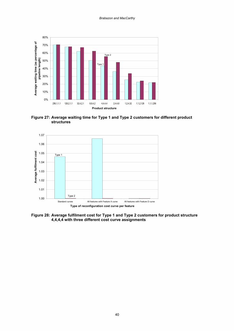
Brabazon and MacCarthy
40
0%
10%
20%
30%
40%
50%
60%
70%
80%
256,1,1,1 128,2,1,1 32,4,2,1 8,8,4,2 4,4,4,4 2,4,4,8 1,2,4,32 1,1,2,128 1,1,1,256
Product structure
Ave
rage
wai
ting
time
(as
perc
enta
ge o
f pi
pelin
e le
ngth
)
Type 1
Type 2
Figure 27: Average waiting time for Type 1 and Type 2 customers for different product
structures
1.00
1.01
1.02
1.03
1.04
1.05
1.06
1.07
Standard curves All features with Feature A curve All features with Feature D curve
Type of reconfiguration cost curve per feature
Ave
rage
fulfi
lmen
t cos
t
Type 1
Type 2
Figure 28: Average fulfilment cost for Type 1 and Type 2 customers for product structure
4,4,4,4 with three different cost curve assignments
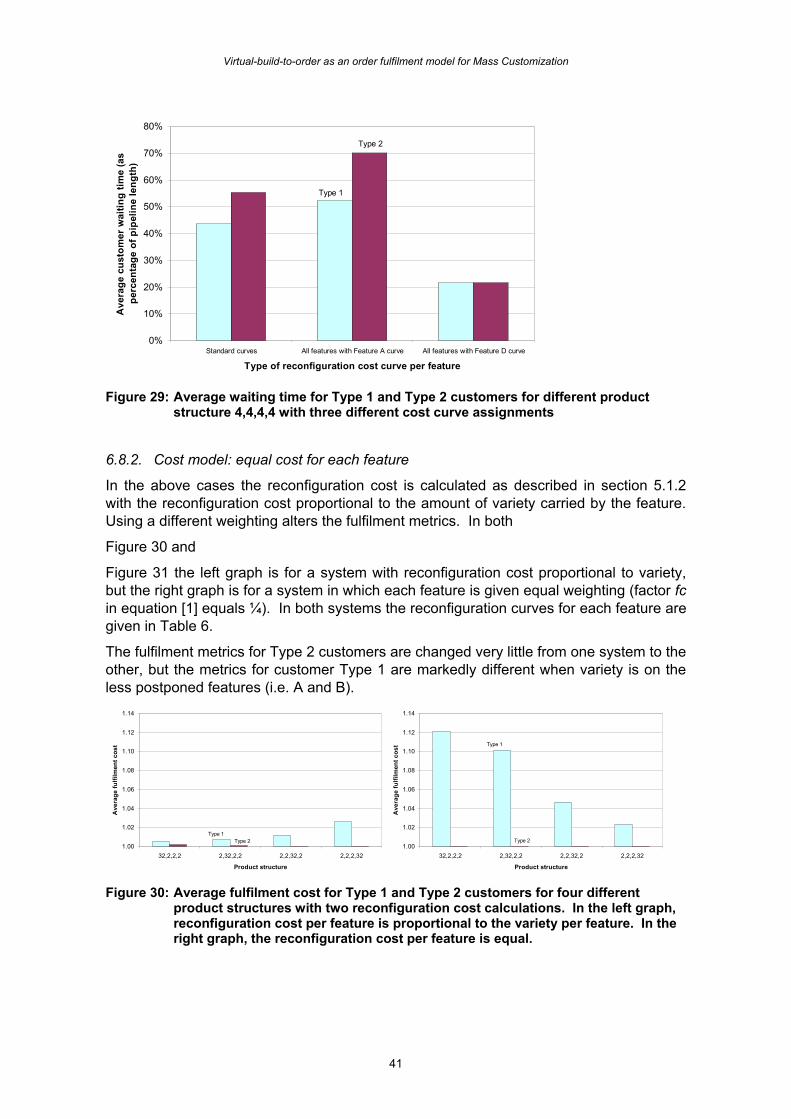
Virtual-build-to-order as an order fulfilment model for Mass Customization
41
0%
10%
20%
30%
40%
50%
60%
70%
80%
Standard curves All features with Feature A curve All features with Feature D curve
Type of reconfiguration cost curve per feature
Ave
rage
cus
tom
er w
aitin
g tim
e (a
s pe
rcen
tage
of p
ipel
ine
leng
th)
Type 1
Type 2
Figure 29: Average waiting time for Type 1 and Type 2 customers for different product
structure 4,4,4,4 with three different cost curve assignments
6.8.2. Cost model: equal cost for each feature
In the above cases the reconfiguration cost is calculated as described in section 5.1.2 with the reconfiguration cost proportional to the amount of variety carried by the feature. Using a different weighting alters the fulfilment metrics. In both
Figure 30 and
Figure 31 the left graph is for a system with reconfiguration cost proportional to variety, but the right graph is for a system in which each feature is given equal weighting (factor fc in equation [1] equals ¼). In both systems the reconfiguration curves for each feature are given in Table 6.
The fulfilment metrics for Type 2 customers are changed very little from one system to the other, but the metrics for customer Type 1 are markedly different when variety is on the less postponed features (i.e. A and B).
1.00
1.02
1.04
1.06
1.08
1.10
1.12
1.14
32,2,2,2 2,32,2,2 2,2,32,2 2,2,2,32
Product structure
Ave
rage
fulfi
lmen
t cos
t
Type 1 Type 2
1.00
1.02
1.04
1.06
1.08
1.10
1.12
1.14
32,2,2,2 2,32,2,2 2,2,32,2 2,2,2,32
Product structure
Ave
rage
fulfi
lmen
t cos
t Type 1
Type 2
Figure 30: Average fulfilment cost for Type 1 and Type 2 customers for four different
product structures with two reconfiguration cost calculations. In the left graph, reconfiguration cost per feature is proportional to the variety per feature. In the right graph, the reconfiguration cost per feature is equal.
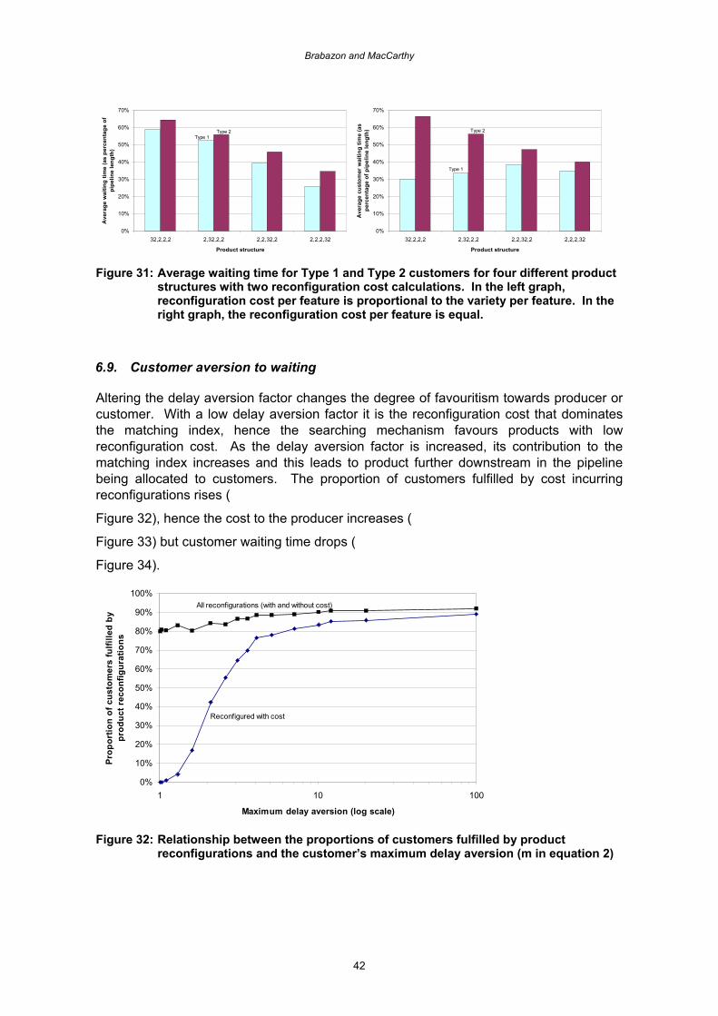
Brabazon and MacCarthy
42
0%
10%
20%
30%
40%
50%
60%
70%
32,2,2,2 2,32,2,2 2,2,32,2 2,2,2,32
Product structure
Ave
rage
wai
ting
time
(as
perc
enta
ge o
f pi
pelin
e le
ngth
)
Type 1 Type 2
0%
10%
20%
30%
40%
50%
60%
70%
32,2,2,2 2,32,2,2 2,2,32,2 2,2,2,32
Product structure
Ave
rage
cus
tom
er w
aitin
g tim
e (a
s pe
rcen
tage
of p
ipel
ine
leng
th)
Type 1
Type 2
Figure 31: Average waiting time for Type 1 and Type 2 customers for four different product
structures with two reconfiguration cost calculations. In the left graph, reconfiguration cost per feature is proportional to the variety per feature. In the right graph, the reconfiguration cost per feature is equal.
6.9. Customer aversion to waiting
Altering the delay aversion factor changes the degree of favouritism towards producer or customer. With a low delay aversion factor it is the reconfiguration cost that dominates the matching index, hence the searching mechanism favours products with low reconfiguration cost. As the delay aversion factor is increased, its contribution to the matching index increases and this leads to product further downstream in the pipeline being allocated to customers. The proportion of customers fulfilled by cost incurring reconfigurations rises (
Figure 32), hence the cost to the producer increases (
Figure 33) but customer waiting time drops (
Figure 34).
0%
10%
20%
30%
40%
50%
60%
70%
80%
90%
100%
1 10 100
Maximum delay aversion (log scale)
Prop
ortio
n of
cus
tom
ers
fulfi
lled
by
prod
uct r
econ
figur
atio
ns
Reconfigured with cost
All reconfigurations (with and without cost)
Figure 32: Relationship between the proportions of customers fulfilled by product
reconfigurations and the customer’s maximum delay aversion (m in equation 2)
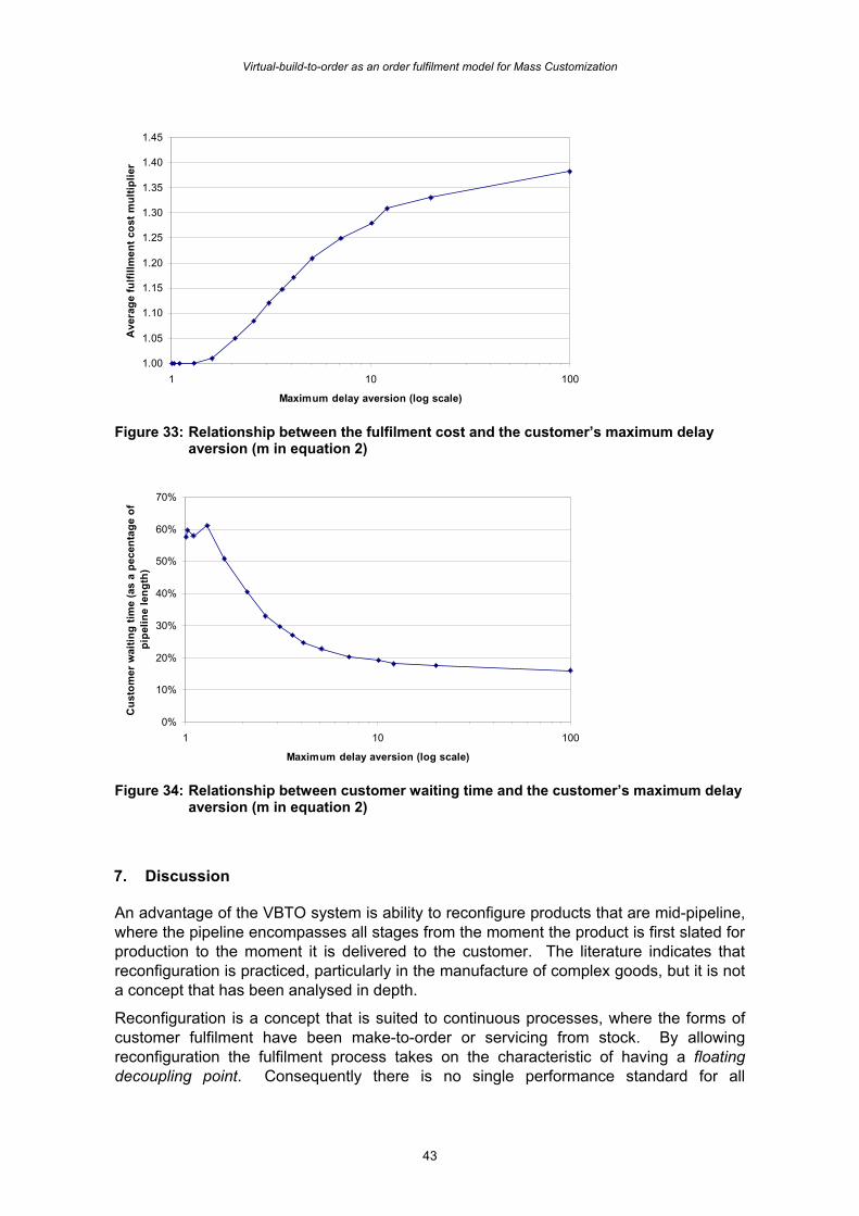
Virtual-build-to-order as an order fulfilment model for Mass Customization
43
1.00
1.05
1.10
1.15
1.20
1.25
1.30
1.35
1.40
1.45
1 10 100
Maximum delay aversion (log scale)
Ave
rage
fulfi
llmen
t cos
t mul
tiplie
r
Figure 33: Relationship between the fulfilment cost and the customer’s maximum delay
aversion (m in equation 2)
0%
10%
20%
30%
40%
50%
60%
70%
1 10 100
Maximum delay aversion (log scale)
Cus
tom
er w
aitin
g tim
e (a
s a
pece
ntag
e of
pi
pelin
e le
ngth
)
Figure 34: Relationship between customer waiting time and the customer’s maximum delay
aversion (m in equation 2)
7. Discussion
An advantage of the VBTO system is ability to reconfigure products that are mid-pipeline, where the pipeline encompasses all stages from the moment the product is first slated for production to the moment it is delivered to the customer. The literature indicates that reconfiguration is practiced, particularly in the manufacture of complex goods, but it is not a concept that has been analysed in depth.
Reconfiguration is a concept that is suited to continuous processes, where the forms of customer fulfilment have been make-to-order or servicing from stock. By allowing reconfiguration the fulfilment process takes on the characteristic of having a floating decoupling point. Consequently there is no single performance standard for all
Brabazon and MacCarthy
44
customers. The fulfilment time and the cost for a customer depends on the state of the system at the time of their arrival.
The ability to reconfigure products mid-pipeline can substantially improve performance in regard to fulfilment time.
Management decisions influence the performance of the VBTO system. The search algorithm for allocating products to customers can be set to favour the producer or the customer. The balance between the producer and customer can be adjusted. Customers can be segmented by means of the delay aversion factor.
8. Future research
Two strands of further research are open. The first is further analysis and modelling of the VBTO system to investigate the implications of factors identified in Table 5. The objectives for this research would be to understand the fundamental relationships between operational and structural factors – pipeline length, product variety – and performance metrics. Particular areas of interest are:
• Behaviour of a two stage customer allocation procedure. Rather than a product being sought and allocated to each customer as they arrive, as has been followed in the present analysis, customers arriving in a time window could be pooled, sorted by priority and then allocated at the end of the window. Of interest is how cost and fulfilment lead times are affected and whether interference between customer types increases or decreases. Because the production system is continuous, too long a window could lead to the build-up of stock, hence holding costs could become a significant factor.
• The comparison of reconfiguration with other fulfilment practices, in particular with specification substitution and specification redundancy.
The second avenue of research is the study of reconfiguration within manufacturing enterprises. A key objective is to develop and apply a protocol for quantifying the reconfiguration cost curve for a feature of a customizable product.
1
References
Agrawal, Mani/ Kumaresh, T.V. / Mercer, Glenn (2001): The false promise of mass customization, The McKinsey Quarterly, Vol 3, pp. 62-71
Alford, D./ Sackett, P. / Nelder, G. (2000): Mass customisation - an automotive perspective, International Journal of Production Economics, Vol 65, No. 1, pp. 99-110
Bartezzaghi, Emilio / Verganti, Roberto (1995): Managing demand uncertainty through order overplanning, International Journal of Production Economics, Vol 40, No. 2-3, pp. 107-120
Bartezzaghi, Emilio / Verganti, Roberto (1995): A technique for uncertainty reduction based on order commonality, Production Planning & Control, Vol 6, No. 2, pp. 157-170
Bi, Z. M. / Zhang, W. J. (2001): Flexible fixture design and automation: Review, issues and future directions, International Journal of Production Research, Vol 39, No. 13, pp. 2867-2894
Boyer, Kenneth K. / Leong, G. Keong (1996): Manufacturing flexibility at plant level, International Journal of Management Science, Vol 24, No. 5, pp. 495-510
Bradley, James R. / Blossom, A. Paul (2001): Using Product-Mix Flexibility to Implement a Make-to-Order Assembly Line, INFORMS International, Hawaii
Brandolese, A. (1990): FlessibilitaÁ e versatilitaÁ nei sistemi produttivi, Economia & Management, Vol 16, No. 5, pp. 47-55
Bucklin, L.P. (1965): Postponement, speculation and the structure of distribution channels, Journal of Marketing Research, Vol 2, No. 2, pp. 26-31
Bukchin, Joseph/ Dar-El, Ezey M. / Rubinovitz, Jacob (2002): Mixed model assembly line design in a make-to-order environment, Computers & Industrial Engineering, Vol 41, No. 4, pp. 405-421
Chang, Dong Shang / Tsou, Ching Shih (1993): A chance-constraints linear programming model on the economic evaluation of flexible manufacturing systems, Production Planning & Control, Vol 4, No. 2, pp. 159-165
Chen, Fangruo (2001): Market Segmentation, Advanced Demand Information, and Supply Chain Performance, Manufacturing & Service Operations Management, Vol 3, No. 1, pp. 53-67
Da Silveira, Giovani/ Borenstein, Denis / Fogliatto, Flavio S. (2001): Mass customization: Literature review and research directions, International Journal of Production Economics, Vol 72, No. 1, pp. 1-13
De Toni, A / Tonchia, S. (1998): Manufacturing flexibility: a literature review, International Journal of Production Research, Vol 36, No. 6, pp. 1587-1617
Dixon, J. R. et al... (1990): The New Performance Challenge: Measuring Operations for World-Class Competition. Irwin.
Duffell, Jeff / Street, Sharon (1998): Mass customisation across the business: Customized production Part 3, Control, Vol 25, No. 1, pp. 24-26
Feitzinger, Edward / Lee, Hau L. (1997): Mass customization at Hewlett-Packard: the power of postponement, Harvard Business Review, Vol 75, No. 1, pp. 116-121
Fine, Charles H. / Freund, Robert M. (1990): Optimal investment in product-flexibile manufacturing capacity, Management Science, Vol 36, No. 4, pp. 449-467
Fogliatto, Flavio S./ Da Silveira, Giovani / Royer, Rogerio (2003): Flexibility-driven index for measuring mass customization feasibility on industrialized products, International Journal of Production Research, Hong KongVol 41, No. 8, pp. 1811-1829
Garg, Amit / Tang, Christopher S. (1997): On postponement strategies for product families with multiple points of differentiation, IIE Transactions, Vol 29, No. 8, pp. 641-650
Gerwin, Donald (1989): Manufacturing Flexibility in the CAM Era, Business Horizons, Vol 32, No. 1, pp. 78-85
Graman, Gregory A. / Magazine, Michael J. (2002): A numerical analysis of capacitated postponement, Production and Operations Management, Vol 11, No. 3, pp. 340-357
Brabazon and MacCarthy
2
Hawkins, Bob (2003): An automotive perspective on Mass Customization - can we Virtually Build to Order?, Mass Customization: Turning customer differences into business advantage, London, UK
Hendry, Linda C. / Kingsman, B. G. (1989): Production planning systems and their applicability to make-to-order companies, European Journal of Operational Research, Vol 40, No. 1, pp. 1-15
Hill, Terry J. (2000): Operations Management: Strategic context and managerial analysis. Palgrave.
Kakati, M (2002): Mass customization - needs to go beyond technology, Human Systems Management, Vol 21, No. 2, pp. 85-93
Koste, Lori L. / Malhotra, Manoj K. (2000): Trade-offs among the elements of flexibility: a comparison from the automotive industry, International Journal of Management Science, Vol 28, pp. 693-710
Kraemer, Kenneth L./ Dedrick, Jason / Yamashiro, Sandra (2000): Refining and extending the business model with information technology: Dell Computer Corporation, Information Society, Vol 16, No. 1, pp. 5-17
Kritchanchai, Duangpun / MacCarthy, Bart L. (1999): Responsiveness of the order fulfilment process, International Journal of Operations and Production Management, Vol 19, No. 8, pp. 812-834
Lee, Hau L. (1996): Effective inventory and service management through product and process redesign, Operations Research, Vol 44, No. 1, pp. 151-159
Lee, Hau L. / Billington, Corey (1995): The Evolution of Supply-Chain-Management Models and Practice at Hewlett-Packard, Interfaces, Vol 25, No. 5, pp. 42-63
Lee, Hau L. / Tang, Christopher S. (1997): Modelling the costs and benefits of delayed product differentiation, Management Science, Vol 43, No. 1, pp. 40-53
Lee, Hau L. / Tang, Christopher S. (1998): Variability reduction through operations reversal, Management Science, Vol 44, No. 2, pp. 162-172
Lindsay, Cotton M. / Feigenbaum, Bernard (1984): Rationing by Waiting Lists, American Economic Review, Vol 74, No. 3, pp. 404-417
Ma, Shihua/ Wang, Wei / Liu, Liming (2002): Commonality and postponement in multistage assembly systems, European Journal of Operational Research, Vol 142, No. 3, pp. 523-538
MacCarthy, Bart L. / Brabazon, Philip G. (2003): Mass customization and quality: the relevance of standard quality techniques, Production Planning & Control, Forthcoming,
Marmorstein, Howard/ Rossomme, Jeanne / Sarel, Dan (2003): Unleashing the power of yield management in the internet era: Opportunities and challenges, California Management Review, Vol 45, No. 3, pp. 147-167
Mccreery, John. K. / Krajewski, Lee. J. (1999): Improving performance using workforce flexibility in an assembly environment with learning and forgetting effects, International Journal of Production Research, Vol 37, No. 9, pp. 2031-2058
Meredith, Jack R./ McCutcheon, David M. / Hartley, Janet (1994): Enhancing Competitiveness through the new market value equation, International Journal of Operations and Production Management, Vol 14, No. 11, pp. 7-22
Norman, George (2002): The relative advantages of flexible versus designated manufacturing technologies, Regional Science and Urban Economics, Vol 32, No. 4, pp. 419-445
Parthasarthy, R. / Sethi, S. P. (1992): The impact of flexible automation on business strategy and organizational structure, Academy of Management Review, Vol 17, No. 1, pp. 86-111
Raturi, Amitabh S./ Meredith, Jack R./ McCutcheon, David M. / Camm, Jeffrey D. (1990): Coping with the build-to-forecast environment, Journal of Operations Management, Vol 9, No. 2, pp. 230-249
Shewchuk, John P. (1999): A set of generic flexibility measures for manufacturing applications, International Journal of Production Research, Vol 37, No. 13, pp. 3017-3042
Virtual-build-to-order as an order fulfilment model for Mass Customization
3
Slack, Nigel (1987): The flexibility of manufacturing systems, International Journal of Operations & Production Management, Vol 7, No. 4, pp. 35-45
Song, Jing -Sheng / Zipkin, Paul (2003): Supply Chain Operations: Assemble-to-Order and Configure-to-Order Systems, in: Graves, S. C. / e Kok, A. G. (eds) Handbooks in Operations Research and Management Science: Design and Analysis of Supply Chains: Elsevier Science Publishers (North Holland)
Swaminathan, Jayashankar M. / Tayur, Sridhar R. (1999): Managing design of assembly sequences for product lines that delay product differentiation, IIE Transactions, Vol 31, No. 11, pp. 1015-1026
Swaminathan, Jayashankar M. / Tayur, Sridhar R. (1998): Managing Broader Product Lines through Delayed Differentiation Using Vanilla Boxes, Management Science, Vol 44, No. 12, pp. S161-S172
Tamura, Takayoshi / Fujita, Seiichi (1995): Designing customer oriented production planning system (COPPS), International Journal of Production Economics, Vol 41, No. 1-3, pp. 377-385
Tamura, Takayoshi/ Fujita, Seiichi / Kuga, Takeo (1997): The concept and practice of the production seat system, Managerial and Decision Economics, Vol 18, pp. 101-112
Tang, Kwei / Tang, Jen (2002): Time-based pricing and leadtime policies for a build-to-order manufacturer, Production and Operations Management, Vol 11, No. 3, pp. 374-392
Tsay, Andy A. / Lovejoy, W. S. (1999): Quantity Flexibility Contracts and Supply Chain Performance, Manufacturing & Service Operations Management, Vol 1, No. 2, pp. 89-111
Tsubone, Hitoshi / Kobayashi, Yoshikazu (2002): Production seat booking system for the combination of make-to-order and make-to-stock products, Production Planning & Control, Vol 13, No. 4, pp. 394-400
Van Mieghem, Jan A. (1998): Investment strategies for flexible resources, Management Science, Vol 44, No. 8, pp. 1071-1079
Vokurka, Robert J. / O'Leary-Kelly, Scott W. (2000): A review of empirical research on manufacturing flexibility, Journal of Operations Management, Vol 18, pp. 485-501
Whang, Seunglin / Lee, Hau L. (1998): Value of Postponement, in: Ho, Teck -Hua / Tang, Christopher S. (eds) Product variety management: research advances: Kluwer Academic Yao, Andrew C. / Carlson, John G.H. (2003): Agility and mixed-model furniture production, International Journal of Production Economics, Vol 81-82, No. 3, pp. 95-102
de Vaal, Albert (2000): Are You Being Served? A General-Equilibrium Analysis of Flexibility in Production, Journal of Economics, Vol 72, No. 1, pp. 19-25
van Hoek, Remko I. (2001): The rediscovery of postponement: a literature review and directions for research, Journal of operations management, Vol 19, No. 2, pp. 161-184