VII. THE DUCTILE/BRITTLE TRANSITION, GAGING DUCTILITY LEVELS In setting out to theoretically characterize and differentiate ductile behavior from brittle behavior it is necessary to first have a credible theory of failure as the starting platform. Historically there was one exceptional mathematical failure criterion and a long list of failures. Perhaps the failures would be better described as mis-guided attempts. In any case, none of them were successful. Only the Mises criterion (and to a much lesser extent the Tresca criterion) for (but only for) ductile metals was an unqualified and very important contribution. All other materials types such as polymers, ceramics, glasses, brittle metals, and minerals did not yield to successful mathematical failure criteria description. The cases of non-metallic materials usually have been approached with empirical failure criteria on a case by case basis. Such empirical forms do not have established limits of validity, and represent little more than curve fits over narrow ranges of data. For a general approach to failure criteria to be successful it must originate from some unifying concept or some special type of physical identification. This will be considered under the next heading, followed by other closely linked subsections on ductility and brittleness. If the vitally important areas of ductile and brittle behaviors are to be realistically treated they must be closely interwoven with a general treatment of failure criteria that applies across the ductile and brittle materials classes. All of these matters will be taken up now. Organizing Principle In searching for an organizing principle for failure criteria, there is an overwhelming example that at least supplies the motivation and inspiration for trying to do so. This is the Periodic Table of the Elements. Its organizing principle is that of the sequence of atomic numbers that then admits further classification when grouped in matrix form with rows and columns.

Is there such a unifying and organizing basis for materials failure? In pursuing this possibility, attention will be focused upon isotropic materials. In scanning across the various materials types, there is an apparent, even obvious differentiation, but still with a connecting thread between them. This difference is that some types of materials have about the same strength in simple tension as in compression, while some others have far less strength in tension than in compression. Still other groups fall in between these two groups. Since the times of antiquity it was always well known and well utilized that gold fell into the first group. It also was learned how to live with the restrictions imposed on the second group for all the common minerals used in ancient construction. However, in the era of failure criteria activity, the realization of the tensile versus compressive strength differences never progressed beyond that point. There only was an awareness of the negative consequences of the possible disparity, no recognition of a possible deeper meaning. The present program of failure characterization is based upon the hypothesis that general isotropic failure behavior is completely organized by and determined by the spectrum of T/C values, where T and C are the uniaxial tensile and compressive strengths. The spectrum of T/C values captures the entire spread from brittle behavior to ductile behavior over the range

0 ! TC! 1

This brittle to ductile change with the variation of the T/C’s is an integral and important part of the organizing structure. Infact, it provides the portal to all further developments. The T/C ratio at a particular value will be referred to as the “materials type”. Thus there is a continuous spectrum of materials types, not just a sequence of discrete groups. The traditional materials groups, polymers, ceramics, etc., have rather specific bands of T/C’s, although there can be and are overlaps. The individual strength properties T and C have very different roles and functions to fulfill in synthesizing the related failure criterion. Both T and C are involved (but unspecified) at the ductile limit of T/C=1. In contrast, only C is involved (but unspecified) at the brittle limit, T/C=0, because T!0. Accordingly it is advantageous to nondimensionalize stress

with respect to C (using T would not be possible) and then have the ensuing failure criterion be expressed entirely in terms of the T/C spectrum.

Following this course take

ˆ ! ij =! ij

C

The organization of failure theory based upon the T/C spectrum does

not automatically determine the failure criterion, but it does indicate that only two properties suffice for the specification. In Sections II and VI the consequent failure criteria for isotropic materials are derived and given in forms that can be put into the following equivalent forms involving only T/C.

The overall failure criterion for homogeneous and isotropic materials

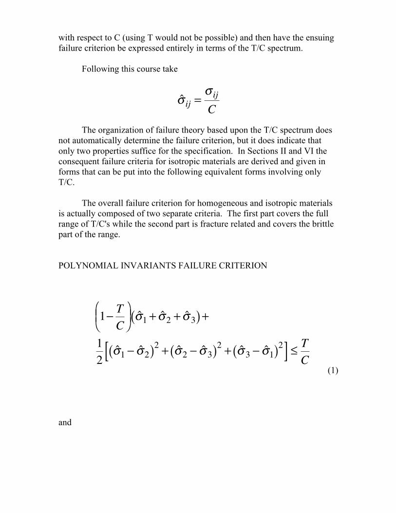
is actually composed of two separate criteria. The first part covers the full range of T/C's while the second part is fracture related and covers the brittle part of the range. POLYNOMIAL INVARIANTS FAILURE CRITERION

1! TC

" # $

% & ' ˆ ( 1 + ˆ ( 2 + ˆ ( 3( ) +

12

ˆ ( 1 ! ˆ ( 2( )2 + ˆ ( 2 ! ˆ ( 3( )2 + ˆ ( 3 ! ˆ ( 1( )2[ ] ) TC

(1) and

COORDINATED FRACTURE CRITERION

ˆ ! 1 "TC

ˆ ! 2 "TC

ˆ ! 3 "TC

#

$

% % %

&

% % %

Also applicable if TC" 1

2 (2)

where principal stresses are employed.

The individual values of T and of C only tell the specific strength properties for a particular material, but it is the T/C ratio that signifies the materials type that is so pivotal in formulating and in interpreting this general theory of failure. A little later the T/C spectrum will also be found to be of first importance in ductile/brittle matters. The two coordinated failure criteria for isotropic materials, (1) and (2), now will be used to develop a framework for characterizing and quantitatively differentiating ductile behavior from brittle behavior. Before doing so, a final observation on the historical search for failure criteria may be in order. Criteria (1) and (2) reduce to the Mises criterion at T/C=1, and they also reduce to a physically meaningful brittle limit at T/C=0. Thus the Mises criterion is a functional part of this general form. The maximum normal stress criterion, originally proposed by Lamé and Rankine, has a superficial resemblance to the fracture criterion (2). If it, (2), were to be considered as a free standing failure criterion, it would be necessary to omit (ignore) the condition for its applicability shown in (2). In some current as well as past sources of information it is stated that the Mises criterion covers ductile materials and the maximum normal stress criterion covers brittle materials. The first half of this assertion is partially correct but the second half of it is completely fallacious. For example, common iron is conventionally considered to be a brittle material. When one compares the maximum normal stress criterion with typical data for the failure of iron, the lack of correlation is glaringly obvious. The comparison of the coordinated failure criteria (1) and (2) with brittle material behavior is quite good, see Section VI.

It is indeed somewhat surprising that this association of T/C values

with the controlling physical behavior was not probed or at least recognized a great many years ago. But that is just a curiosity, a footnote to history. Building up a viable theory of behavior is another matter entirely and only the latter counts for anything, anytime. Characterizing Ductility The conventional methods for characterizing ductility and brittleness are as follows. Brittleness is usually taken to be the sudden, unexpected interruption of the linear elastic stress strain loading form. Not only is this “unannounced” failure occurrence annoying, it often is dangerous, sometimes extremely dangerous. Some warning of impending failure would be tremendously helpful. This simple classification of idealized brittle behavior will suffice for initial purposes. Ductility is much more complex. The usual method of identifying ductility is with imposed uniaxial tension. If the material proceeds with a strain hardening state after exceeding some yield stress, and if it is capable of experiencing large strains in that state then it is said to be ductile. This view is unduly restrictive and it certainly doesn’t suffice for describing ductility for three dimensional stress states. There is a need for a more inclusive definition of ductility. For present purposes, relevant examples of brittle and ductile behaviors are given in Fig. 1.

Fig. 1 Failure types

In these diagrams, " and # are taken to represent any stress strain loading state, one, two, or three dimensional. But the progressive loading is always taken to be of the proportional type. That Case (i) is brittle is obvious. So too is Case (iii) obviously ductile. However, Case (ii) is where the complexity arises. Case (ii) is crucial, and will first be approached in the manner now shown. The distinguishing characteristic of ductility is here taken to be the capacity to absorb mechanical energy and convert it into irrecoverable heat energy, or involve some other irreversible damage process. Perhaps the best way to characterize ductility is that it involves mechanical energy dissipation, which is completely absent in the case of idealized brittle failure. Obviously Case (ii) has a smaller degree of ductility than does Case (iii). How important is this? Any ductility is much more than no ductility. Even in this sense, a small degree of ductility is very helpful and it affords an important capacity for damage tolerance. In non-uniform stress states, e. g. stress concentrations, some ductility allows material mobility to adjust to local conditions without causing macroscopic failure. With the above considerations in mind, Case (ii) will be taken with the following method of broadly (not precisely) distinguishing ductile from brittle behavior. Fig. 2 shows Case (ii) with some designations.

Fig. 2 Failure designations

The conditions of brittle versus ductile behavior are taken to satisfy

! f "# f

E, Brittle

! f >> # f

E, Ductile

These forms give a general and conventional threshold for ductile behavior. In the second of these, the strain at failure may be as little as only 30 or 40 or 50% greater than the elastic projection, for there to be the inception of significant ductility. Otherwise, the mechanical failure behavior is taken to be brittle as in Case (i) or close to it. So brittle behavior allows a moderate generalization beyond that shown in Case (i). Still, there is a “grey” area, an uncertain area, in between the behaviors of totally brittle and ideally ductile types. Also, this operational definition of and distinction between ductile and brittle behaviors is stress state dependent, and it is taken to apply to all stress states.

Again, it should be emphasized that even a small degree of ductility can be extremely advantageous, especially as compared with idealized brittle behavior, Case (i). These designations will suffice for having a physical understanding of the possible and likely differences between ductile and brittle behaviors. The clear message is that ductile versus brittle failure behavior is not just an on/off switch. There is a graded and graduated change from one to the other. To say these are difficult matters would be an understatement. They pose long standing, classically difficult, unresolved issues.

The fundamental task is that of quantifying ductility levels. None of this so far accomplishes that purpose. To make progress on theoretically gaging ductility levels requires a drastic change in direction and approach from the vague and rather loose traditional discussions of ductility at the macroscopic level. Now a new direction will be sought. In so doing, it should be recognized that any real improvement in characterizing ductility (or lack of) for homogeneous materials must be applicable to all stress states, not just carefully selected, particular ones. The Ductile/Brittle Transition, the Failure Number for Gaging Ductility Levels A given material is generally taken to be ductile or brittle based upon experience and exposure. In this heuristic but eminently practical approach, ceramics are said to be brittle, some metals are brittle and some are ductile, and polymers are “all over the place”. There is nothing inherently wrong with intuitive and practical approaches but it is likely that there could be a more organized approach to this problem. First there should be some measurable but nondimensional physical characteristic(s) that determines the materials type as it relates to its expected failure type, ductile or brittle. Not surprisingly this missing identifier will here be taken to be the strength ratio T/C. But if one tries to use only the T/C tag to make general assertions about ductile versus brittle failure, one must also ask if this could be true under all conditions. It is quickly seen that there must be qualifiers, especially that of the stress state under which the failure characteristic is to be determined. Generally tensile type stress states are far more likely to promote brittle behavior, for a given material, than are generally compressive type stress states. The objective here is to find a rational

method for classifying and quantifying expected failure behavior, ductile or brittle with appropriate gradations in between, based upon the materials type, specified by T/C, and the specific imposed state of stress at failure. In the papers containing archive references given in Section II and discussed in Section VI, a criterion for ductile versus brittle failure is given as

I1 < 3T !C , Ductile

I1 > 3T !C , Brittle (3)

where

I1 = !11f +!22

f +! 33f is the first invariant in terms of the failure

stresses. These relations, for specified values of T and C then designate which stress states are expected to represent brittle failure and which ones have ductile failure. The first invariant is at its value on the failure envelopes (1) or (2) and thus expressed in terms of T and C for the imposed stress state. Now express relations (3) in non-dimensional form for further use here,

ˆ ! iif < 3T

C"1 , Ductile

ˆ ! iif > 3T

C"1 , Brittle

(4)

where

ˆ ! iif is the nondimensionalized first invariant of the failure stress state

from (1) or (2). The relations in (4) actually only give the transition from ductile to brittle conditions when the inequalities are replaced by an equality. Thus, for a particular stress state the value of T/C can be found at which the stress state is at the borderline between ductile and brittle failures but it tells nothing about the relative scales of ductility or brittleness in general failure conditions. It will be helpful to recall here the outline of the derivation of (4). Take the two dimensional state of biaxial failure stresses as shown in Fig. 3.

Fig. 3 Ductile/Brittle Transition, 2-D example

Relations (1) and (2) produce the intersection of failure modes shown in Fig. 3. The domain is divided into ductile and brittle regions at the intersection of the failure modes, as shown. If the ductile brittle division were taken through the other intersection corners nearer the origin in Fig. 3 it would quickly be found to lead to unacceptable results. This process is repeated, taking T/C as a continuous variable to find the functional relationship between T/C and the division into ductile and brittle regions. The functional relationship is then taken to continue into the range where T/C$1/2. The end result is the ductile/brittle criteria, (4). The fact that this ductile/brittle division is at the intersection of failure modes (1) and (2) requires that this be done in two dimensional stress space as a subspace of three dimensional stress space. It cannot be done

unambiguously in one dimensional or directly in three dimensional spaces. Deriving the ductile/brittle criteria in this way in two dimensional space leaves the one dimensional and three dimensional behaviors to be critically examined for verification of predicted behavior using test results. This has been done in Section VI, although much more testing could be done along these lines. As a simple example of relations (4) consider the case of the failure stress in simple shear. Take S as this failure stress. Using relations (1) and (2) and (4), along with S/T=(S/C)(C/T) gives the result in Fig. 4.

Fig. 4 Shear stress failure types The change in failure mode type as well as the type of failure (ductile or brittle) occurs at T/C=1/3 for a state of simple shear. It is important to visualize the ductile/brittle criteria (4) in three dimensional, principal stress space. The failure criterion (1) takes the form of a paraboloid in principal stress space. The fracture criterion, for T/C%1/2, cuts off “slices” from the paraboloid, leaving three flattened surfaces on it. The ductile/brittle criteria (4) at the transition represents a plane which is

normal to the axis of symmetry of the paraboloid. The ductile/brittle transition plane from (4) is given by

ˆ ! iif = 3T

C"1 , D /B Transition (5)

This plane divides the failure surface into ductile and brittle regions as shown in Fig. 5 for the example T/C=0, the brittle limit.

Fig. 5 Ductile/Brittle Transition, 3-D example

Even in this limit case, T/C=0, there still are separate ductile and brittle regions. This will be further discussed a little later. At any T/C value, the ductile/brittle plane cuts across the three elliptical flattened surfaces (when they exist, T/C % 1/2) at their 1/4 points nearest the apex of the paraboloid. It would not be expected that the ductile/brittle transition at any T/C value is of a sharp nature. This is not a first order thermodynamic transition. The significance of this division boundary is that the proclivities toward ductile versus brittle failure are in balance, while on either side of the division the weighting gradually shifts to a dominate effect, one way or the other. Planes of equal but unspecified ductility would be parallel to the ductile/brittle transition plane defined by (5). It would be advantageous to have the means to characterize the degree of ductility (or lack of it) for particular failure states on either side of the D/B transition plane. To this end, rewrite (5) in an alternative form. Take & to be specified by

! = 3TC" ˆ # ii

f "1 (6)

When &=0 (6) just reverts back to the criterion (5) for the transition. But when &'0, (6) has an interpretation as a measure of the degree of ductility or brittleness, as will be shown. This is not surprising since it is already known that &=0 is one point on the ductility/brittleness scale. Positive values of & reflect ductility, while negative values indicate brittleness. For a fixed value of T/C, & represents a measure of distance from the ductile/brittle transition plane to the parallel plane containing the stress state of interest. Examine the case of uniaxial tension. For this stress state

ˆ ! iif =T/C

and so (6) gives

! = 2 TC"1

For the range on T/C as 0 % T/C % 1 then

!1" # " 1 Also, it should be noted that for uniaxial tension the ductile/brittle transition is at T/C=1/2. The stress state of uniaxial tension is the only one that has

these matching symmetry forms on T/C and on &. Uniaxial tension will be taken as the baseline stress state, and all other stress states will be calibrated relative to it. It comprises the basic template for characterizing ductility. The value &=1 corresponds to full, perfect ductility, while &= -1 corresponds to total brittleness Now consider the state of simple shear stress. In this case

ˆ ! iif =0 and

(6) becomes

! = 3TC"1

For uniaxial tension the ductile /brittle transition value of T/C=1/2 gives &=0. But for simple shear the same T/C=1/2 value gives &=1/2. This means that at this value of T/C, simple shear failure is more ductile than is uniaxial tensile failure. And at T/C=2/3, then for simple shear &=1, the fully ductile situation. Thus for the case of simple shear, values of T/C larger that 2/3 simply remain as fully, perfectly ductile at &=1. Any stress state that at a particular value of T/C gives a value of & larger than 1 will be assigned as fully ductile, at &=1. Correspondingly any stress state with a value of & less than -1 will be taken as totally brittle at &= -1. In effect, the planes of perfect ductility and total brittleness are located at fixed distances from the D/B plane for all T/C’s.

It is convenient to rescale the quantity &. For -1 % & % 1, change the variable so that the new scale goes from 0 to 1. To this end, take

Fn = 12! +1( )

or using (6)

Fn = 12

3TC! ˆ " ii

f# $ %

& ' ( (7)

Consistent with taking & at limits of -1 and 1, as totally brittle or perfectly ductile respectively, the new quantity Fn will revert to the limits of 0 or 1 when its value from (7) is outside these limits. So always

0 ! Fn ! 1

Calibrating to the uniaxial tension stress state is the only one that then gives Fn=1/2 at the T/C values for the ductile/brittle transitions of all the stress states.

A slightly different form of (7) is that of

Fn = 32TC! ˆ " m

f# $ %

& ' ( (7a)

where

ˆ ! mf is the nondimensionalized mean normal stress at failure.

The quantity Fn will be called the failure number. It represents a measure of ductility, with Fn=0 being no ductility, total brittleness, and Fn=1 being full, perfect ductility. Rather than expressing Fn within the 0 to 1 interval, it will always be stated as the corresponding percentage, from 0 to 100%. For Fn=50% the material is at the ductile/brittle transition. This is the 50-50 case as regards ductility versus brittleness. For Fn below 50% brittleness begins to dominate, while for Fn above 50% ductility begins to dominate.

The procedure for using the failure number is as follows. The sum of the three normal stresses at failure,

ˆ ! iif , are found from the failure theory

(1) and (2) or they may be taken directly from experimental data. These are then put into the failure number formula, (7). The two simplest examples are uniaxial tension and compression. The former has

ˆ ! iif =T/C and the

latter has

ˆ ! iif =-1. Putting these into (7) gives the corresponding failure

numbers as functions of T/C. These can then be evaluated at specific values of T/C to ascertain the related ductility level. The table below shows the values of T/C for the ductile/brittle transition and the failure number formulas for some basic stress states.

Stress State D/B Transition T/C

Failure Number Fn

Uniaxial Tension 1/2

TC

Uniaxial Comp. 0

123TC

+1! " #

$ % &

Simple Shear 1/3

32TC! " #

$ % &

Eqi-Biaxial Ten. 1

1+ T2C

! 1! TC

+ TC" # $

% & ' 2

Eqi-Biaxial Comp. Always Ductile

1+ T2C

+ 1! TC

+ TC" # $

% & ' 2

Eqi-Triaxial Ten. Always Brittle

TC1! 32TC" # $

% & '

( ) *

+ , -

1! TC

Table 1 Failure Numbers, Fn

There are no failures in eqi-triaxial compression in this failure theory. Next the failure numbers for various stress states are arranged in descending order, thus going from the most ductile stress state to the least ductile, most brittle stress state. Cases over the full range of T/C’s are given.

Table 2 gives a comprehensive view of the ductility levels of the failure mechanisms as a function of the stress state and the materials type. It is the state of uniaxial tension, not shear, that anchors the results. The state of uniaxial tension is of fundamental and singular importance in calibrating the ductile/brittle behavior for all isotropic materials.

It is seen that insofar as ductile versus brittle failure behavior is concerned the sensitivity to the stress state type is just as great as the sensitivity to the materials type. It must be recognized that there are very large differences in failure behavior for materials below the 50% ductility level from those above it. For example, for the uniaxial tensile stress state, the ductility level of 25% would be in the range of T/C’s for ceramics, while the 75% level would be representative of T/C’s for very ductile polymers. The large majority of cases in Table 2 are at or below the ductility level of 50% indicating problems with expected brittle behavior.

It also is apparent in Table 2 that cases below and to the left are

dominated by brittle behavior, while those above and to the right are ductile. It is thus possible to identify ductile versus brittle failure mode groupings as a function of materials type and stress state. The key to this division are the cases at the 50% level, the ductile/brittle transition. All of the 50% values are exactly at Fn=1/2.

In the four cases in Table 2 at T/C=0 with no ductility, total

brittleness, it should be remembered that the corresponding stress levels allowed by the failure criteria are at zero, so the ductility levels are irrelevant. However this does show that exceedingly small T/C’s would have virtually total brittleness. The one case at T/C=0 with a specified ductility level reflects the fact that even at T/C=0 a compressive mean normal stress component does stabilize the material and give an allowable failure stress level with a corresponding ductility level. It is generally true that for a given stress state, the ductility increases with increasing values of T/C. However, such simple rules become invalid when comparing different stress states. For example, from Table 2 it is seen that a T/C=1/3 material in simple shear is more ductile than a T/C=2/3 material in eqi-biaxial tension. Another set of examples involves more complicated stress states than those given in the above tables. Consider two possible stress states where the principal stresses at failure are in the proportions

1 : 23:! 23

and

1 : 23: 13

It is of interest to know which one is the more ductile of the two stress states, and by how much. To proceed further it is necessary to specify the material of interest. Take the material as a typical, fairly ductile epoxy resin with

TC

= 35

= 0.6

As the first step, note from (7) that the failure number for this epoxy in uniaxial tension is

Fn = 60% , Uniaxial tension, epoxy It will be of relevance to not only compare the failure numbers for the two stress states with each other, but also with that for the material in uniaxial tension, which comprises the base line. The answers to these questions of relative ductility levels are certainly not obvious. All three stress states will be shown in the comparison. Using the Fn formula (7) and the failure criteria (1) and (2) it is found that

Case

!1 :! 2 :! 3

ˆ ! 1f , ˆ ! 2

f , ˆ ! 3f Fn

Uniaxial Ten. 1 : 0 : 0 3/5, 0, 0 60%

I 1 : 2/3 : -2/3 3/7, 2/7, -2/7 69%

II 1 : 2/3 : 1/3 3/5, 2/5, 1/5 30%

Table 3 Failure numbers for 3-D stress states at T/C=0.6

It is seen from this table that Case I is on the ductile side of the scale and Case II is on the brittle side. Judging from the values of the Fn’s the differences in the degrees of ductility are huge. Furthermore, Case I, the ductile case, is even more ductile than the epoxy its self is in uniaxial tension. All of these results would be purely guesswork without the rationale of the failure number, Fn.

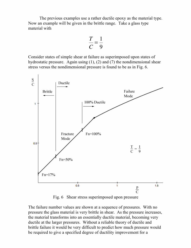
The previous examples use a rather ductile epoxy as the material type. Now an example will be given in the brittle range. Take a glass type material with

TC

= 19

Consider states of simple shear at failure as superimposed upon states of hydrostatic pressure. Again using (1), (2) and (7) the nondimensional shear stress versus the nondimensional pressure is found to be as in Fig. 6.

Fig. 6 Shear stress superimposed upon pressure

The failure number values are shown at a sequence of pressures. With no pressure the glass material is very brittle in shear. As the pressure increases, the material transforms into an essentially ductile material, becoming very ductile at the larger pressures. Without a reliable theory of ductile and brittle failure it would be very difficult to predict how much pressure would be required to give a specified degree of ductility improvement for a

particular material. It also follows that a state of superimposed hydrostatic tension can convert a ductile material into an essentially brittle one. It is also interesting to note that the change of failure mode and the ductile/brittle transition are not coincident, Fig. 6. Although such coincidence does occur in two dimensional stress states, as explained earlier it does not occur with three dimensional stress states. Thus there is a large region of ductile fracture evident in Fig. 6. The failure number, as specified by (7) and by failure criteria (1) and (2) does give a scale or ranking for the degree of ductility of different stress states for any particular isotropic material specified by its T/C value. This is somewhat like the role and function of the Reynolds number for fluids. Both the Reynolds number, Re, and the failure number, Fn, provide gages upon the expected behavior due to control/domination by an inherent nonlinear physical effect, inertial in the former case and failure in the latter. The difference is that the Reynolds number is for broad classes of flow types while the failure number is explicit and specific to any particular failure mode.

It would not be expected that the failure number would have the same widespread appeal as the Reynolds number does, it is a little too complicated for that. But Fn does reveal that there is an underlying logical basis for expecting and predicting degrees of ductility in failure as a function of the materials type and the imposed state of stress. No less than that should be expected from any legitimate and comprehensive failure criterion. Furthermore, the failure criteria (1) and (2) and the failure number (ductility level), (7), are very amenable to use with finite element codes in design. Although the main thrust of this website was outlined in the introductory section, Section I, it is worth briefly repeating it here. This “book” explores, delineates, and codifies the main aspects of three dimensional failure criteria for materials. It does not take the place of peer reviewed archive papers, rather it builds upon such contributions. As such, this work involves interpretations of the subtleties of materials failure behavior. Nowhere are the difficulties more complex or more subtle than with characterizing ductility and its deleterious complement, brittleness.

Richard M. Christensen

June 27th 2010

Copyright © 2010 Richard M. Christensen