· Web viewJEL Classification: C23, R23 Área Anpec: 10 – Economia Regional e Urbana A Spatial...

A Spatial Economic Model and Spatial Econometric Analysis of Population Dynamics in Brazilian MCAs

Diego Firmino Costa da SilvaFederal University of Pernambuco and University of Groningen. Address: Rua Dr. Odilon Lima, 44/02, 50850-010, Afogados, Recife, PE, Brazil. E-mail: [email protected], Phone: +55 (81) 32711196

J. Paul ElhorstUniversity of Groningen. Address: P.O. Box 800, 9700 AV, Groningen, the Netherlands. E-mail: [email protected], Phone: +31503633893

Raul da Mota Silveira NetoFederal University of Pernambuco. Address: Av. Prof. Moraes Rego, 1235, Recife, PE, 50670-901, Brazil. E-mail: [email protected], Phones: +55 (81) 21268381 r. 224, + 55 (81) 91381357

AbstractTo extend existing theoretical population growth models, this article proposes including spatial interaction effects. Using data pertaining to 3659 Brazilian Minimum Comparable Areas (MCA) over the period 1970-2010, this extension is tested by estimating a dynamic spatial panel model. The authors also compare the performance of a wide range of potential neighborhood matrices using Bayesian posterior model probabilities. Six of the thirteen determinants of population growth considered produce significant spatial interaction effects. Moreover, five produce significant long-term spatial spillover effects; a mathematical analysis reveals the strength of this result, which requires more than a single parameter. Treating areas as independent entities, as many previous population growth studies have done, underestimates the impact of various policy measures.Keywords: Population growth, regions, spatial interaction, dynamic spatial panel models, spillover effects

ResumoO trabalho analisa os condicionantes do crescimento das cidades brasileiras no período 1970-2010, apresentando para tal três inovações com respeito à literatura nacional e internacional sobre crescimento das cidades. Primeiro, a partir da incorporação de interações espaciais, o trabalho propõe uma extensão dos modelos econômicos utilizados para explicar o crescimento das cidades. Segundo, como teste empírico do modelo, o trabalho utiliza informações sobre o crescimento populacional das Área Mínimas Comparáveis Brasileiras no período 1970-2010 em um painel especial dinâmico. Por fim, utiliza estimações Bayesianas para a escolha das especificações espaciais mais adequadas. Os resultados obtidos indicam que seis dos treze condicionantes do crescimento populacional apresentam interações espaciais (cidades afetadas pelas variáveis dos vizinhos), com cinco deles apresentando efeitos de longo prazo, o que está de acordo com o modelo proposto e revela a importância da consideração de interações espaciais no estudo do crescimento das cidades brasileiras. Palavras-chave: Crescimento populacional, regiões, interacões espaciais, painel espacial dinâmico, spillover.

JEL Classification: C23, R23Área Anpec: 10 – Economia Regional e Urbana

A Spatial Economic Model and Spatial Econometric Analysis of Population Dynamics in Brazilian MCAs

1. Introduction Brazilian urbanization represents a highly significant, robust social phenomenon, such that

through the vast economic and social changes of the past four decades, the percentage of people living in urban centers in Brazil has grown steadily. According to the last Brazilian Demographic Census (2010), it increased from 55.9% in 1970 to 84.4% in 2010 (IBGE, 2011). This process resulted largely from improved economic and social prospects in cities (Da Mata et al., 2007; Henderson, 1988; Yap, 1976), though Ramalho and Silveira-Neto (2012) also note that the most important migration of people in Brazil since the 1990s has occurred among cities. Thus, beyond demographic factors, the key sources of the population growth dynamics of Brazilian cities are associated with specific urban characteristics.

Yet we know relatively little about how these specific factors condition this population growth. Henderson (1988) shows that the population growth of Brazilian cities between 1960 and 1970 related positively to initial increases in levels of education. Reviewing growth between 1970 and 2000, Da Mata et al. (2007) reveal that favorable supply and demand conditions, including market potential variables, better schooling, and limited opportunities in the agricultural sector, favored the growth of Brazilian cities. However, similar studies have not extended to more recent periods, which feature some notable shifts. After a decade of high inflation, the early 2000s offered a period of price stability, as well as income convergence among Brazilian states (Silveira-Neto and Azzoni, 2012). Substantial increases in the production of commodities and agricultural goods during this period also had positive impacts on opportunities available in towns further distant from large urban centers. In addition, Da Mata et al. (2007) focus on municipalities with more than 75,000 inhabitants, or about 75% of Brazil’s urban population. They do not model or test for any spatial dependence of population growth dynamics among Brazilian cities. Yet spatial dependence is particularly severe for small spatial units, such as municipalities (Boarnet et al., 2005). In analyzing income dynamics at different levels of spatial aggregation, Resende (2013) confirms the importance of spatial dependence for Brazilian minimum comparable areas (MCA).1

The Brazilian Constitution of 1988 states that the municipality is the third and lowest political administrative unit of the country, with autonomy to collect taxes on service activities (ISS: Imposto sobre Serviços) and urban real estate property (IPTU: Imposto Predial e Territorial Urbano), as well as to legislate land use. These policies potentially affect the location of firms and people, such that they might generate reactions from or affect neighboring cities (Brueckner, 2008). Furthermore, spatial technological spillovers (Ertur and Koch, 2007) may be more prevalent among small, urban, neighboring centers than among large ones. By considering spatial urban centers on a lower, fuller scale, we consider the possibility that common or shared amenities affect the population’s welfare.

Because we assert that all of these factors might induce spatial dependence on the population growth dynamics of Brazilian cities and its determinants, we seek to model spatial dependence among spatial units explicitly. Our central objective is to present the population growth dynamics of Brazilian MCAs and thereby assess the determinants of the population growth of these units between 1970 and 2010, as well as examine the existence and magnitude of spatial interaction and spatial spillover effects associated with these determinants. To model the population growth dynamics of Brazilian cities (MCA), we construct an economic–theoretical model that includes spatial interaction effects, then estimate this model using dynamic spatial panel techniques, with controls for spatial and time-specific effects. Accordingly, we can disentangle the magnitude and significance levels of spatial spillover effects, in both the short and the long term, and guarantee that any support for these effects is not simply an artifact of ignoring time-specific effects that areas have in common. Almost half of our explanatory variables reveal significant spatial interaction and spatial spillover effects, namely, rural population size, population

1 A MCA is a municipality or aggregation of municipalities necessary to enable consistent spatial analyses over time; we provide more details in Section 4.2.

2

density, and birth, literacy, and homicide rates. These significant spatial interaction and spillover effects indicate that the impact of policy measures that act on these variables tends to be considerably underestimated (by up to 60%) by non-spatial approaches that treat MCAs as independent entities.

In the next section, we motivate our investigation by presenting a spatial extension of the city population growth model developed by Glaeser (2008), which accounts for spatial interaction effects among productivity and city amenities and also implies an empirical specification for population growth dynamics that consists of spatial interaction effects in the dependent and independent variables. In Section 3, we present the econometric methodology underlying our empirical investigation. We also introduce spatial interaction effects and define spatial spillover effects. After we detail our data set in Section 4, we present the results of the empirical analysis in Section 5. Finally, we summarize our main findings and draw conclusions.

2. A Spatial Extension of Glaeser’s Population Growth Model

Our theoretical framework of population growth across Brazil builds on previous work by Glaeser et al. (1995), Brueckner (2003), and Ertur and Koch (2007). In the urban growth model developed by Glaeser et al. (1995),2 cities are independent economies that share common pools of labor and capital and differ in their level of productivity (Ait) and quality of life (Qit). The total output of an economy depends on the productivity level, which can be modeled as a Cobb-Douglas production function that depends on population size. The total welfare of a potential migrant to this economy equals wages multiplied by the quality of life, which decreases with population size. The net result is a population growth regression that contains several factors that determine quality of life, including crime, housing prices, traffic congestion, population size, and productivity growth.

An objection to this theoretical framework is that it ignores spatial interaction effects among economies, especially between a locality and its surroundings. To address this problem, we could increase the scale of the geographical units in the empirical analysis, with the assumption that interaction effects at this higher scale no longer exist (Glaeser et al. 1995). Another, more prevalent option is to model spatial interaction effects explicitly. Suppose the total output of an economy is given by

Y it=Ait Pitβ K it

γ Z̄i1−β−γ , (1)

where Pit represents the population size in economy i at time t, Kit denotes traded capital, and Z̄i is fixed non-traded capital. Then, the first extension includes productivity interaction effects among economies. Ertur and Koch (2007) argue that knowledge accumulated in one economy depends on knowledge accumulated in other economies, though with diminished intensity due to frictions caused by socio-economic and institutional dissimilarities, which in turn can be captured by geographical distance or border effects. More formally,

Ait=ait∏j≠i

N

a jtρw ij

, (2)

where the productivity level of an economy Ait depends on urban differences in the productivity of labor related to social, technological, and political sources in the own economy i ait, as well as those in neighboring economies j ajt; in addition, N is the number of economies. The parameter ρ reflects the degree of interdependence among economies, with 0 < ρ < 1. Although this parameter is assumed to be identical for all economies, the impact of the interaction effects on economy i depends on its relative location, reflecting the effect of being located closer to or further away from other economies. This

2 A more sophisticated approach that also includes the housing market is available in Glaeser (2008).3

relative location can be represented by the exogenous term wij, which is assumed to be non-negative, non-

stochastic, and finite, establishing an N N neighborhood matrix W in which 0≤w ij≤1 and w ij=0 if i = j. By substituting Equation (2) into Equation (1), we find that the total output of an economy is given by

Y it=(ait ∏j≠i

N

a jtρwij) Pit

β K itγ¯ Z i1− β−γ

. (3)

The first-order conditions for capital and labor, that is, capital income (normalized price = 1) and labor income (denoted Sit ) are equal to their marginal products, yield the following labor demand equation, as long as the optimal solution for capital is substituted in the condition for labor:

Sit=βγγ

1−γ (ait ∏j≠i

N

a jtρw ij)

11−γ P it

β+γ−11−γ ¯Z i

1−β−γ1−γ

. (4)

As this labor demand equation shows, higher wages reflect higher productivity and fewer workers.Consumers also have Cobb-Douglas utility functions for tradable goods and housing, denoted by

Cit and Hit, respectively. We can assume that welfare is due, at least partly, to the (dis)amenities of the local economy Θit. The locality's (dis)amenities directly affect the welfare of people who live there; they might interfere negatively or positively with a resident’s utility, and they can be either natural (e.g., climate, beaches, vegetation) or generated by humans (e.g., violence, entertainment, traffic, pollution). Formally, U it=C it

1−α H itα Θit , (5)

where α is a constant. The price of tradable goods is normalized to 1; the housing price is pH. Consumers maximize their utility, subject to a budget constraint

C it+ pH H it=S it , (6)

by choosing Cit and Hit.Our second extension includes amenity interaction effects across economies. Some (dis)amenities

may (dis)benefit persons living in other economies (Brueckner, 2003). For example, people might use facilities in other localities; the violence in a particular neighborhood can generate feelings of insecurity in adjacent neighborhoods; and water pollution can cause health damages downstream. In mathematical terms,

Θit=(θit∏j≠i

N

θ jtηw ij) , (7)

where the overall amenities of an economy Θit depend on local amenities θit and those in neighboring economies θjt, and the impact of the latter decreases with geographical distance. The parameter η measures the degree of interdependence among economies, with 0 < η < 1. According to Glaeser et al. (1995), many potential (dis)amenities can be reflected by the level of population and the population growth rate; the greater the size of a city, the lower the quality of life. The costs of migration rise with the number of immigrants, and if the population size increases rapidly, expansions in public goods, infrastructure, and housing might not be able to keep pace. Therefore, residents of quickly growing cities suffer in terms of quality of life, yielding the utility function

4

U it=C it1−α H it

α(θ it∏j≠i

N

θ jtηwij)P it

−ϕ( P it

Pit−1 )−τ

, (8)

where ϕ>0 and τ>0 . In addition, total city demand for housing is given by

H D=Pit

αSit

pH . (9)According to Glaeser and Gottlieb (2009), the spatial equilibrium condition is a primary theoretical tool for urban economists, as exemplified in pioneering work by Mills (1967), Rosen (1979), and Roback (1982) on population changes within a country. This condition states that utility equalizes across space, provided that labor is mobile; higher wages in urban areas get offset by negative urban attributes, such as higher prices and negative amenities. If the common utility level at a particular point in time is denoted by V̄ t , application of the spatial equilibrium condition produces the following results when we substitute the demand equation for housing derived in Equation (9) into Equation (8), such that it yields the indirect

utility function in Equation (10), equal to V̄ t :

V ( Sit , pH )=α (1−α )1−α(θit ∏j≠i

N

θ jtηwij)S it pH

−α Pit−ϕ ( Pit

P it−1 )−τ

=V̄ t. (10)

Following Glaeser (2008), housing floor space is produced competitively, either by land (L) or by height (h). A fixed quantity of land at a particular location (L̄ ) determines an endogenous price for land (pL) and housing (pH), and the cost of producing hL units of structure on top of L units of land is given by c0hδ L , where δ >1 . The developer then maximizes profits, π=pH hL−c0 hδ L−pL L . (11)

The first-order condition of this maximization problem for height, h=( pH /δc0)1

δ−1, implies the total

housing supply equation:

h L̄=( pH /δc0 )1

δ−1 L̄ . (12)By comparing housing demand in Equation (9) with housing supply in Equation (12), we can obtain the housing price equation:

pH=( Pit αSit

L̄ )δ−1

δ (δc0 )1δ

. (13)Labor demand in Equation (4), indirect utility in Equation (10), and housing prices in Equation

(13) then form a system, with three unknown variables (Pit, Sit, and pH). Solving this system for the population Pit yields

log Pit=DN+ψ {logθit +(η∑j≠i

N

w ij logθ jt )+(δ−αδ−αδ )(log ait +ρ∑

j≠i

N

w ij log a jt) +τ log P it−1+ log { V̄ ¿¿ t } , (14a)where

ψ=δ (1−γ )

(1−γ ) (α (δ−1)+δϕ+δτ )−(δ−αδ+α )(β+γ−1) , and (14b)

5

DN=ψ (α log α+(1−α ) log (1−α )+(δ−αδ−αδ )(log β+(γ

1−γ ) log γ+(1−β−γ1−γ ) log { Z̄ ¿)

−α (δ−1)δ −

αδ log (δc0 )+(α (δ−1)

δ ) log { L̄

) . ¿

(14c)According to Glaeser and Gottlieb (2009), the spatial equilibrium condition means that in a

dynamic model, only lifetime utility levels get equalized across space. However, as long as housing prices or rents can change quickly, or to a reasonable extent within the observation periods being considered— which is 10 years for the present study3—a price adjustment is enough to maintain the spatial equilibrium.

Then the change in utility between times t and t +1 is the same across space, V̄ t+1

V̄ t , and Equation (14a) can be rewritten as

log( Pit+1

Pit )=ψ ( log (θit+1

θit )+(η∑j≠i

N

w ij log(θ jt+1

θ jt ))+(δ−αδ−αδ )(log (ait+1

ait )+ρ∑j≠i

N

wij log(a jt+1

a jt )) + τ log (Pit

Pit−1 )+log (V̄ t+1

V̄ t )) . (15)

Following Glaeser et al. (1995), we also assume that Xit is a vector of city characteristics at time t that determine both city-specific amenity growth and the growth of city-specific productivity:

log ( θ it+1

θit)=X it

' λθ, and (16a)

log( ait+1

ait)=X it

' λa. (16b)

Combining Equations (14) and (16), we derive the dynamic spatial population growth equation:

log ( Pit+1

P it)=ψalignl [τ log ( Pit

Pit−1 )+(1+(δ−αδ+α )

δ ) X it' ( λθ+λa )¿]¿

¿

¿¿

(17a)

log( Pit+1


Pit−1 )+(1+(δ−αδ+α )

δ ) X it' ( λθ+λa )¿]¿

¿

¿¿

(17b)

The equation (17a) contains spatial interaction effects among both the explanatory variables. Empirically, there is the possibility of spatial interaction among the error terms, as showed in equation (17b). In spatial econometrics literature, such a model specification in (17b) would be known as the spatial Durbin error model (SDEM; see LeSage and Pace, 2009). The right-hand side of this model also contains the dependent variable, lagged one period, so it also could be labeled a dynamic SDEM model.

3 Duranton and Puga (2013) cite cyclical behavior and sluggish adjustment as reasons to measure population growth over periods of five or ten years.

6

The utility function specified in Equation (8) assumes that the quality of life for potential migrants declines with both the level and the growth rate of the population. Just as knowledge and amenities in one economy interact with knowledge and amenities in others, so might the level and growth rate of population depend on these values in neighboring economies. If residents of quickly growing cities suffer in terms of quality of life, they might move to neighboring areas. Therefore, assuming individual utility correlates negatively with the level of population (population size) and the population growth rate of neighbors, the utility function takes the form

U it=C it1−α H it

α(θ it∏j≠i

N

θ jtηw ij)P it

−ϕ( P it

Pit−1 )−τ

(∏j≠i

N

P jt−νwij)(∏j≠i

N

( Pit

Pit−1 )−σw ij)

, (18)

where ν>0 and σ>0 . Solving the system for the population Pit with this alternative specification of the utility function yields a population growth equation, as follows:

log ( Pit+1


Pit−1 )+σ∑j≠i

N

wij log ( P jt

P jt−1)− (ν+σ )∑j≠i

N

wij log ( P jt+1

P jt )+ ¿][(1+ δ−αδ+αδ )X it

' (λθ+λa) ¿ ]¿¿

¿¿

(19a)

log ( N it +1

N it)=ψalignl [τ log( N it

N it−1 )+σ∑j≠i

N

wij log( N jt

N jt−1 )−(ν+σ )∑j≠i

N

wij log( N jt+1

N jt )+ ¿][(1+ δ−αδ +αδ ) X it

' ( λθ+ λa ) ¿]¿¿

¿¿

(19b)

where ψ is defined as in Equation (14b). In addition to spatial interaction effects among the explanatory variables, this model specification also contains spatial interaction effects among the dependent variable. Empirically, there is the possibility of spatial interaction among the error terms, as showed in equation (19b). In the spatial econometrics literature, such a model specification in (19b) is known as the general nesting spatial model (GNS) model (Elhorst, 2014), and if we account for the dependent variable lagged one period, it is a dynamic GNS model.

3. Econometric MethodologyThe econometric counterpart of the dynamic spatial GNS model, which is the final equation

implied by the theoretical model presented in the previous section, reads, in vector form, as

Yt = τYt-1+δWYt+ηWYt-1+Xtβ+WXtθ+μ+λtιN+vt, vt=λWvt+εt, (20)

7

where Yt denotes an N 1 vector that consists of one observation of the dependent variable for every economy (i = 1, ..., N) in the sample at time t (t = 1, ..., T), which for this study is the population growth rate, log(Pit+1/Pit); and Xt is an N K matrix of exogenous or predetermined explanatory variables, observed at the start of each observation period. A vector or matrix with subscript t–1 in Equation (20) denotes its time lagged value, whereas a vector or matrix premultiplied by W denotes the spatially lagged value. The N × N matrix W is a non-negative matrix of known constants that describe the spatial arrangement of the economies in the sample, as introduced in the previous section. The parameters τ, δ, and η are the response parameters of, respectively, the dependent variable lagged in time Yt-1, the dependent variable lagged in space WYt, and the dependent variable lagged in both space and time WYt-1. The symbols β and θ represent K 1 vectors of the response parameters of the exogenous explanatory variables. Although we tried to maintain consistent symbols, the limited supply of Greek letters mandated that many of the parameters in the econometric model relied on a different interpretation than those used in the theoretical model, as set out in the previous section. The error term specification consists of different components: the vector vt that is assumed to be spatially correlated with autocorrelation coefficient λ; the N 1 vector εt = (ε1t, …, εNt)T that consists of i.i.d. disturbance terms, which have zero mean and finite variance 2; the N 1 vector μ = (μ1, …, μN)T that contains spatial specific effects i and is meant to control for all spatial-specific, time-invariant variables whose omission could bias the estimates in a typical cross-sectional study (Baltagi, 2005); and time-specific effects λt (t = 1, …, T), where ιN is a N × 1 vector of ones, meant to control for all time-specific, unit-invariant variables whose omission could bias the estimates in a typical time-series study. Such spatial- and time period–specific effects generally can be treated as fixed or random effects, but as Elhorst (2014) notes, a random effects model in the cross-sectional domain might not be an appropriate specification if observations of adjacent units in an unbroken study area are being used and the whole population is sampled. In contrast, a random effects model would make sense if a limited number of MCAs were being drawn randomly from Brazil, but in that case the elements of the neighborhood matrix could not be defined, and the impact of spatial interaction effects could not be estimated consistently. Only when neighboring units are part of the sample is it possible to measure the impact of neighboring units. Therefore, this study is distinct from urban studies that seek to explain economic growth in cities, such as those by Glaeser et al. (1995) and Da Mata et al. (2007).4 We include both urban and rural regions, to cover the whole country and model the interactions, whereas previous studies ignore the potential interaction effects with surroundings and treat cities as independent entities.

Direct interpretation of the coefficients in the dynamic GNS model is difficult, because they do not represent true partial derivatives (LeSage and Pace, 2009). Debarsy et al. (2011) and Elhorst (2012a) show that the matrix of (true) partial derivatives of the expected value of the dependent variable with respect to the kth independent variable for i = 1, …, N in year t for the short term is given by

[∂ E(Y )∂ x1 k

⋯∂ E(Y )∂ x Nk ]t=( I −δW )−1 [ βk I N+θk W ]

. (21)In addition, LeSage and Pace (2009) advocate for decomposing the marginal effects into direct

(own-economy) and indirect (spillover) effects. The direct effects stem from the own-partial derivatives along the diagonals in Equation (21); they reflect the effects on the dependent variable that results from a change in the kth regressor xk in economy i in the short term. The off-diagonal elements represent short-term indirect effects. Because the direct and indirect effects differ across units in the sample, LeSage and Pace (2009) propose one summary indicator for the direct effects, measured by the average of the diagonal elements, and another summary indicator for the indirect effects, measured by the average of the column sums of the non-diagonal elements of that matrix. The matrix reflecting the right-hand side of Equation (21) is independent of the time index t, so these calculations are equivalent to those presented by LeSage and Pace (2009) for a cross-sectional setting. From Elhorst (2012a), it follows that the long-term marginal effects are given by

4 A recent overview is available in Duranton and Puga (2013).8

[∂ E(Y )∂ x1 k

⋯∂ E(Y )∂ x Nk ]=[(1−τ ) I −(δ +η)W ]−1 [ βk I N+θk W ]

. (22)Thus, by examining the relationship between population growth and its determinants using the

decompositions in Equations (21) and (22), we can disentangle direct and indirect effects into short- and long-term effects.

One problem with the dynamic GNS model is that its parameters are not identified, as acknowledged by Anselin et al. (2008), Gibbons and Overman (2012), and Elhorst (2014). The interaction effects among the dependent variable and the error terms cannot be distinguished formally, as long as the interaction effects among the explanatory variables are also included, unless the neighborhood matrix takes the form of a group interaction matrix—a specification rarely used in applied spatial econometric research. Therefore, one of the two spatial interaction effects seemingly should be excluded, if we hope to obtain consistent parameter estimates. If the spatial interaction effects for the dependent variable are excluded, the dynamic SDEM specification results, consistent with the utility function specified in Equation (8). Then δ = η = 0, and the spatial multiplier matrix (I – δW)-1 in Equation (21) reduces to the identity matrix, while the spatial multiplier matrix [(1 – τ)I – (δ + η)W]-1 in Equation (22) reduces to the matrix 1/(1 – τ)I.

If we leave aside the spatial interaction effects among the error terms, a dynamic spatial Durbin model (SDM) results. This model specification is consistent with the utility function specified in Equation (18). Although the specification does not account for interaction effects among the error terms, which reduces the efficiency of the parameter estimates, it does not affect the consistency of the parameter estimates. Imposing the restriction λ = 0 also does not influence the direct or indirect effects derived in Equations (21) and (22). As LeSage and Pace (2009) note, the cost of ignoring spatial dependence in the dependent and/or independent variables is relatively high, because if one or more relevant explanatory variable gets omitted from a regression equation, the estimator of the coefficients for the remaining variables is inherently biased and inconsistent (Greene, 2005). In contrast, ignoring spatial dependence in the disturbances, if present, only leads to a loss of efficiency.

Another important difference between the SDEM and SDM specifications is that the indirect or spatial spillover effects in the first model are local, whereas in the second model, they are global in nature. Anselin (2003) clarifies this difference: In the SDM specification, a change in X at any location gets transmitted to all other locations, following the inverse matrix in Equation (21), if the two locations are unconnected according to W. Local spillovers instead occur at other locations, without involving an inverse matrix, that according to W are connected only to each other.

To choose between SDM and SDEM specifications, and thus between the utility functions specified in Equations (8) or (18) and a global or local spillover model, we apply a Bayesian approach (LeSage, 2013). A Bayesian perspective is appropriate, considering the model uncertainty. By addressing the marginal likelihood of the SDM and SDEM models, and thereby integrating out all parameters of the model, we can calculate the Bayesian posterior model probabilities of the SDM and SDEM specifications, conditional on the sample data. With two models, we have p(SDM|Y,X,W) + p(SDEM|Y,X,W) = 1. If the probability of one model is greater than that of the other, we can conclude that it describes the data better, because the comparison is based on the same set of explanatory variables, both model specifications include X and spatially lagged X (denoted by WX) variables, and the comparison is independent of the integrated out, specific parameter values.

With this Bayesian perspective, we also can test different specifications of the neighborhood matrix W against each other. Formally, tests for significant differences between log-likelihood function values, such as the likelihood ratio (LR) tests, cannot apply if models are non-nested (i.e., based on different neighborhood matrices); Bayesian methods do not require nested models to achieve these comparisons. By repeating the previous analysis for different specifications of the neighborhood matrix and comparing their performance on the basis of the value of the log-marginal likelihood, we can identify the neighborhood matrix that outperforms other potential specifications.

9

Depending on the outcomes of these tests, we finally estimate either the SDM or the SDEM specification, using maximum likelihood (ML). If the test points to the dynamic SDM, it can be estimated using the bias-corrected ML estimator developed by Yu et al. (2008) and Lee and Yu (2010), depending on whether time period fixed are included. If it points to the dynamic SDEM, the model can be estimated with the bias-corrected ML estimator developed by Elhorst (2005).

4. Data ImplementationOur data come from the Brazilian Demographic Census for the years 1970, 1980, 1991, 2000, and

2010, as conducted by the Brazilian Institute of Geography and Statistics (IBGE), complemented by data collected by the Brazilian Institute for Applied Economic Research (IPEA).

The municipality constitutes the lowest administrative level in Brazil for which economic and demographic data are available. During 1970–2000, the number of municipalities increased from 3,952 to 5,565. Such ongoing changes in the number, area, and borders of municipalities mean that a consistent comparison over time is possible only if we aggregate the municipalities into broader geographical areas, or MCAs. Using the aggregation of municipalities developed by IPEA (Reis et al., 2010), we obtain a spatial panel of 3,659 MCAs during 1970–2010 (see also Da Mata et al., 2007). Therefore, we refer consistently to MCAs hereafter.

With Equations (17), (19), and (20), we measure the dependent variable of our empirical analysis Yit by the rate of population growth in one particular MCA over a decade (t – 1, t), where i runs from 1 to 3,659, t in Equation (20) spans from 1980 to 2010, and the number 1 represents a decade. This population growth rate depends on the population growth rate in the previous decade; when we use the dynamic spatial Durbin model, it also depends on the population growth rate in neighboring units in contemporaneous and previous decades. Noting our theoretical model (Section 2) and data availability, we consider the influences of 13 explanatory variables, whose selection reflected the recent review by Duranton and Puga (2013) and previous studies by Glaeser et al. (1995), Da Mata et al. (2007), and Chi and Voss (2010).

In particular, Duranton and Puga (2013) discuss key theories from urban growth research and their implications in terms of population, surface area, and income per person. They provide empirical evidence of the main drivers of city growth, drawn primarily from the Unites States and other developed countries. Although Brazil is an emerging economy, and we consider population growth in both urban and rural areas to be able to model spatial interaction effects, the explanations put forward in their overview remain helpful for selecting explanatory variables for the present study. However, the variables selected must be revised for the different context. For example, whereas Duranton and Puga (2013) observe a tendency to measure human capital by the share of university graduates, we focus on the share of people aged 25 years and over who are literate, a measure that is more meaningful in Brazil and that increased from 48% in 1970 to 82% in 2010. We also integrate Glaeser et al.’s (1995) contribution, considering that their work provided the theoretical basis for our spatial extension in Section 2. We value Da Mata et al. (2007) for its empirical focus on population growth in Brazil, though it includes only 123 Brazilian agglomerations and does not span the whole country. Both Glaeser et al. and Da Mata et al. also ignore spatial interaction effects, such as those between an agglomeration and its surroundings or between a city and its suburbs within an agglomeration. Finally, we rely on Chi and Voss (2011), because it estimates a dynamic spatial panel data model, though without providing a theoretical motivation for this model specification.

Two of the key drivers of city growth that Duranton and Puga (2013) identify are infrastructure and housing supply. The first follows from the monocentric city model; the second determines how cities react to positive or negative shocks. If the supply of houses is limited by geographical constraints or land-use regulations, a positive shock leads to higher housing prices. If the supply of houses is elastic, housing prices might increase to some extent, but the local inhabitants and incoming migrants react by choosing to live in smaller dwellings. Important infrastructural components of the housing supply in Brazil are the proportions of people with access to public water or public sewers; insufficient supply may cause higher prices and deter potential migrants. These two variables also appear in Chi and Voss’s (2010) study,

10

whereas Glaeser et al. (1995) consider expenditures on sanitation. These variables increased from, respectively, 14% and 5% in 1970 to 71% and 37% in 2010. Population density can control for the second factor. Many cities could take in more people, though at the expense of the quality of the living conditions, which might deter prospective migrants. Because it takes time to build public goods, infrastructure, or housing, the residents of quickly growing cities may suffer more in terms of their quality of life.

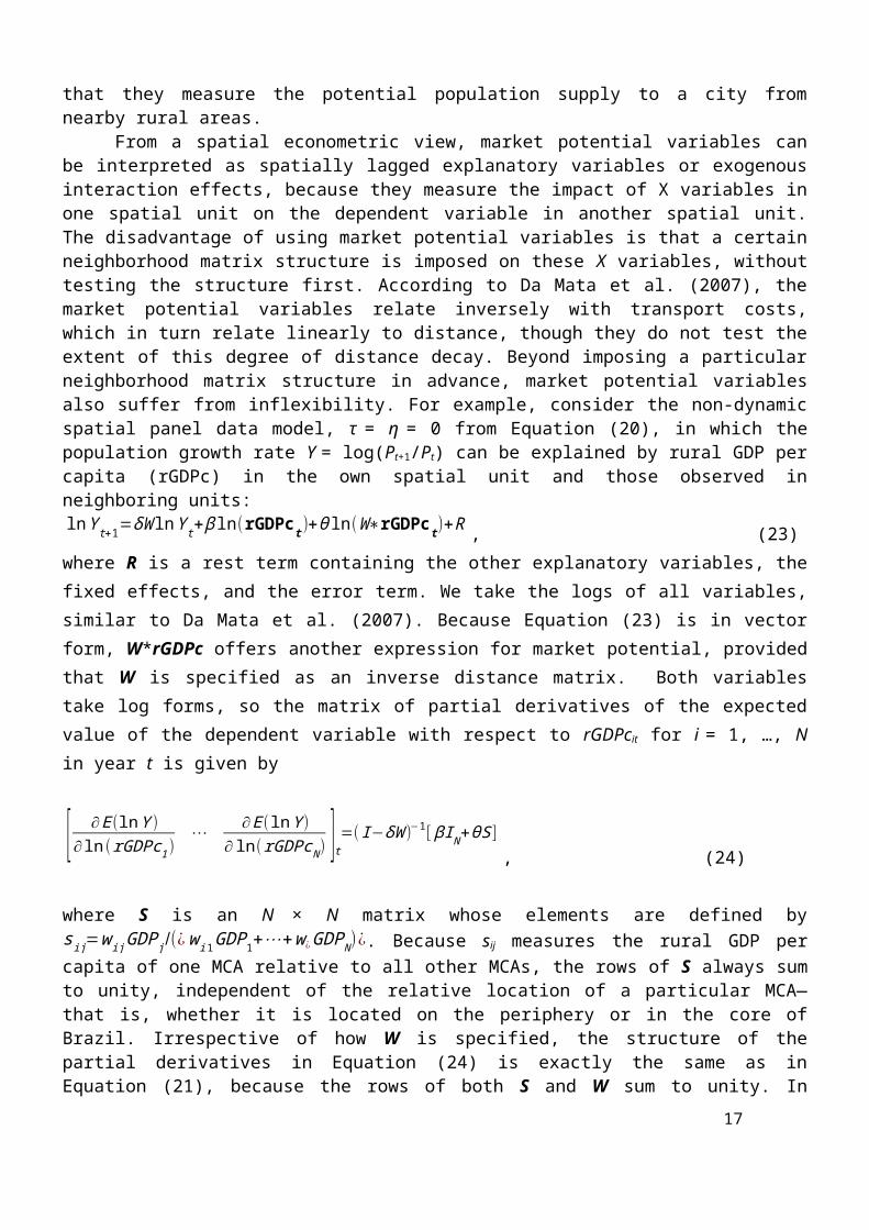
According to Duranton and Puga (2013), the availability of road infrastructure is another important component, and agglomeration effects drive city growth. Da Mata et al. (2007) argue that city growth depends on demand and supply factors, which they summarize as the incomes a city can pay out and the incomes people demand to live in a city, respectively. To measure these factors, they use market potential variables, which depend partly on road transport networks. The demand market potential of a spatial unit in turn is defined as the product of per capita income and population size, divided by transport costs, summed over all spatial units in the sample. To describe the supply side, they consider two gravity measures for each spatial unit: the sum of per capita rural income divided by transport costs over all other spatial units in the sample, and the sum of the rural population divided by transport costs over all other spatial units in the sample. Both constitute market potential measures, in that they measure the potential population supply to a city from nearby rural areas.

From a spatial econometric view, market potential variables can be interpreted as spatially lagged explanatory variables or exogenous interaction effects, because they measure the impact of X variables in one spatial unit on the dependent variable in another spatial unit. The disadvantage of using market potential variables is that a certain neighborhood matrix structure is imposed on these X variables, without testing the structure first. According to Da Mata et al. (2007), the market potential variables relate inversely with transport costs, which in turn relate linearly to distance, though they do not test the extent of this degree of distance decay. Beyond imposing a particular neighborhood matrix structure in advance, market potential variables also suffer from inflexibility. For example, consider the non-dynamic spatial panel data model, τ = η = 0 from Equation (20), in which the population growth rate Y = log(Pt+1/Pt) can be explained by rural GDP per capita (rGDPc) in the own spatial unit and those observed in neighboring units:ln Y t +1=δW ln Y t+ β ln (rGDPct )+θ ln (W∗rGDPct )+R , (23)where R is a rest term containing the other explanatory variables, the fixed effects, and the error term. We take the logs of all variables, similar to Da Mata et al. (2007). Because Equation (23) is in vector form, W*rGDPc offers another expression for market potential, provided that W is specified as an inverse distance matrix. Both variables take log forms, so the matrix of partial derivatives of the expected value of the dependent variable with respect to rGDPcit for i = 1, …, N in year t is given by

[ ∂ E( lnY )∂ ln (rGDPc1 )

⋯∂ E ( lnY )

∂ ln (rGDPcN ) ]t=( I−δW )−1 [ βI N+θS ], (24)

where S is an N × N matrix whose elements are defined by sij=wij GDP j /(¿w i 1GDP1+⋯+w ¿GDPN )¿. Because sij measures the rural GDP per capita of one MCA relative to all other MCAs, the rows of S always sum to unity, independent of the relative location of a particular MCA—that is, whether it is located on the periphery or in the core of Brazil. Irrespective of how W is specified, the structure of the partial derivatives in Equation (24) is exactly the same as in Equation (21), because the rows of both S and W sum to unity. In contrast, by replacing ln(W*rGDPc) with W*ln(rGDPc) and decomposing the composite variables, such as market potential, into their underlying components (which leads to partial derivatives similar to those in Equation (21)), we introduce more empirical flexibility, including the opportunity to test how W should be specified and thus to what extent MCAs likely interact. Furthermore,

11

the magnitudes of the direct and indirect effect estimates can vary with different explanatory variables that determine the market potential. Just as in Da Mata et al. (2007), we assume that the population growth rate depends on GDP per capita, rural GDP per capita, rural population size, and their spatially lagged values, but as separate variables, so that we can test for agglomeration effects.

We also control for other demand and supply factors: the industry mix and the size of the workforce. Glaeser et al. (1995) control for the share of employment in manufacturing and find that it has an adverse effect on population growth. Da Mata et al. (2007) control for the ratio between the share of employment in manufacturing to that of services, to account for local adjustments relative to changes in national output composition, and find a positive effect. Chi and Voss (2011) include the share of employment in agriculture, though they removed this variable from the model when it emerged as insignificant. Yet we still control for the share of employment in agriculture, because we focus on population growth in Brazil, with its vast agricultural areas; especially at the beginning of our observation period, the number of women in the labor force was relatively high, mostly as unpaid workers on family farms who combined their agricultural work with childcare. When income levels started to rise, such as through the expansion of the manufacturing sector and the introduction of new technologies, women’s labor force participation rates tended to fall (Goldin 1995; Mammen and Paxson, 2000). Men moved into new blue-collar jobs that increased family-level income, such that unearned income effects reduced women’s participation. In summary, we expect that the share of employment in agriculture has a negative effect on population growth, due to the reduction in economic opportunities, especially for women. Similar to Da Mata et al. (2007), we control for the ratio between the share of employment in manufacturing and that of services.

Glaeser et al. (1995) also control for unemployment, because potential migrants do not move to areas with high unemployment rates. They find an adverse effect on U.S. population growth after 1970; we thus use the percentage of the economically active population that is occupied as an additional supply side factor. This variable offers an opposite of the unemployment rate.

Although GDP per capita measures often appear in empirical growth studies, they ignore a critical dimension of population dynamics, namely, populations' evolving age structure. Each age group in a population behaves differently, and the distribution across age groups changes over time, so economic opportunities can be boosted or slow down temporarily. Whereas prime-age adults supply labor and savings, the young require education, and the aged need health care and retirement income. Economic opportunities then should increase when the number of working-age adults is large, relative to the dependent population, but decrease when a population rapidly ages. By translating an economic model formulated as GDP per capita growth into a comparable model of GDP per worker, which largely determines demand and supply conditions in a city and its surroundings, different studies have shown that demographic variables might be important (Bloom and Williamson, 1998; Choudhry and Elhorst, 2010; Kelley and Schmidt, 2005). Such variables include the mean age of the population and the birth rate. If the population of a particular region is relatively immobile, differences in population growth across areas within that region likely are due mainly to differences in fertility (Glaeser et al., 1995), which is an important reason to consider the birth rate.

Finally, according to Duranton and Puga (2013), (dis)amenities drive city growth. Da Mata et al. (2007) explicitly mention local crime and violence, measured by the homicide rate or number of homicides per one million inhabitants. This variable exerts a negative and significant effect on population growth in their study, so we include it in the present study as well.

5. Empirical AnalysisThe estimation results are in Table 1. The first column reports the estimation results of a standard

linear panel data model, extended to include spatial and time-period fixed effects, but without any spatial interaction effects. We discuss the results of several specification tests before turning to the estimation results in the second column of Table 1.

Table 1. Population Growth: Non-Spatial and Dynamic Spatial Models12

OLS + Time- and Spatial-

Specific Fixed Effects Dynamic SDM + Fixed

Effects (bias correction)Explanatory Variables Coeff t Coeff t Spatial tlagged population growth rate -0.0271 *

* 0.0755** 0.0681

**

ln rural population -0.0433 ** -0.0391

** 0.0068

Density -0.1248 ** -0.1256

**

-0.0221

**

mean age 0.0135 ** 0.0089

**

-0.0020

birth rate 0.0172 ** 0.0150

** 0.0072

**

literacy rate 0.1361 ** 0.0681

** 0.0395

agriculture -0.2612 ** -0.2315

** 0.1063

**

manufacturing/service 0.0045 ** 0.0021

** 0.0016

occupied workforce 0.4911 ** 0.3535

**

-0.0681

ln GDP per capita 0.0513 ** 0.0527

**

-0.0248

**

ln rural GDP per capita 0.0088 ** 0.0135

**

-0.0095

**

homicide rate -0.0030 ** 0.0006

-0.0042 *

water company 0.0081 0.0274-

0.0255

sewer company -0.0123 -0.0365**

-0.0058

WY (delta) 0.3439**

No. Obs. 10977 10977R-squared 0.711 0.743

Log Likelihood 111445580.3

7Spatial lag, OLS model:

LM 909.32 ** Spatial lag, SDM model:

LM(robust) 114.89 ** Wald 54.39

**

Spatial error, OLS model:

LM 796.34 ** Spatial error, SDM model:

LM(robust) 1.91 Wald 134.23 *13

*Joint significance

LR(spatial fe=0) 8674.60**

LR(time fe=0) 789.06**

** Significant at 1%. *Significant at 5%.

To investigate the (null) hypothesis that the spatial fixed effects are jointly insignificant, we performed a likelihood ratio (LR) test. The results (8674.34, with 3658 degrees of freedom [df], p < 0.01) reject this hypothesis. Similarly, we can reject the hypothesis that the time-period fixed effects are jointly insignificant (789.06, 3 df, p < 0.01). These results justify the extension of the model with spatial and time period fixed effects. Table 2 reports the correlation coefficients for the explanatory variables, which indicate that multicollinearity is not a problem.

Table 2. Correlation Coefficients Across Explanatory Variablesln rural population 1.00

ln density -0.25 1.00

mean age -0.32 0.13 1.00

birth rate -0.29 -0.16 -0.05 1.00

literacy rate -0.30 0.14 0.60 -0.15 1.00

agriculture 0.23 -0.32 -0.31 0.21 -0.48 1.00

manufacturing/services -0.09 0.11 0.14 -0.07 0.20 -0.19 1.00

workforce occupied 0.09 -0.04 -0.29 0.14 -0.20 0.48 -0.08 1.00

ln GDP per capita -0.26 0.19 0.40 -0.13 0.76 -0.42 0.19 -0.07 1.00

ln rural GDP per capita 0.10 -0.44 0.02 0.19 0.05 0.46 -0.07 0.38 0.20 1.00

homicide rate -0.05 0.17 0.02 -0.13 0.14 -0.25 -0.03 -0.19 0.18 -0.19 1.00

water company -0.36 0.26 0.56 -0.18 0.65 -0.64 0.11 -0.40 0.55 -0.20 0.18 1.00

sewer company -0.30 0.26 0.51 -0.13 0.53 -0.45 0.11 -0.22 0.49 -0.10 0.07 0.641.0

0

To test whether the non-spatial model with spatial and time period fixed effects should be extended with spatial interaction effects for the dependent variable (SAR specification) or for the error terms (SEM specification), we used LM tests, applied to a first-order, binary, contiguity neighborhood matrix that we row-normalized to ensure row sums equal to 1. These LM tests follow a chi-squared distribution with one degree of freedom and reach a critical value of 3.84 at 5% significance or 2.71 at 10% significance. In classic LM tests, the hypotheses of both no spatially lagged dependent variable and no spatially autocorrelated error term must be rejected. With robust tests, we can reject the hypothesis of no spatially lagged dependent variable, but the hypothesis of no spatially autocorrelated error term cannot be rejected, at 10% significance. These test results suggest extending the non-spatial model with a spatially lagged dependent variable. However, if the robust LM tests reject a non-spatial model, in favor of the spatial lag or spatial error models, we must carefully endorse one of these models. LeSage and Pace (2009) and Elhorst (2012b) also recommend considering the spatial Durbin model and testing whether it can be simplified to the spatial lag or spatial error model. For this study, we take a broader view and apply the Bayesian approach from Section 3. First, we calculate the Bayesian posterior model probabilities of the SDM and SDEM specifications, as well as the simpler SAR and SEM specifications, to identify which model specification best describes the data. Second, we repeat this analysis for several specifications of the neighborhood matrix, to find the specification of W that best describes the data. In

14

total, we consider 11 matrices: p-order binary contiguity matrices for p = 1–3, an inverse distance matrix, and q-nearest neighbors matrices for q = 5–10 and 20.

Table 3. Comparison of Model Specifications and Neighborhood MatricesW Matrix Statistics SAR SDM SEM SDEM

Binary Contiguity log marginal 3566.85 3616.03 3548.42 3611.80model probabilities 0.0000 0.9855 0.0000 0.0145

First and Second Order log marginal 3562.21 3574.79 3558.60 3579.41model probabilities 0.0000 0.0097 0.0000 0.9903

First, Second and Third Order log marginal 3527.98 3528.75 3535.86 3536.28model probabilities 0.0001 0.0003 0.3974 0.6022

Inverse distance log marginal 3368.78 3444.87 3363.32 3455.44model probabilities 0.0000 0.0000 0.0000 1.0000

5 nearest neighbors log marginal 3539.69 3601.04 3521.72 3597.88model probabilities 0.0000 0.9594 0.0000 0.0406







Source: Own calculations, based on LeSage (2013)

The results in Table 3 show that the SAR and SEM models are always outperformed by either the SDM or SDEM specifications. Therefore, spatially lagged explanatory variables (WX) are important and should be included in the model. The worst performing spatial weight matrix is the inverse distance matrix, which corroborates our point that decomposing market potential variables into their underlying components and considering the spatially lagged values of these components creates a much greater degree of empirical flexibility. If the neighborhood matrix is specified as a first-order binary contiguity matrix or as a 5-nearest neighbors matrix, the Bayesian posterior model probabilities point to the SDM specification. The average number of neighbors in the sample amounts to 4.98, so these two neighborhood matrices are not substantially different. If we let the number of neighbors increase, by considering either higher-order binary contiguity matrices or nearest neighbors matrices with more neighbors, the Bayesian posterior model probabilities provide further evidence in favor of the SDEM specification. However, by also considering the log-marginal values of the different specifications of the spatial weight matrix, we note that the first-order binary contiguity matrix and the SDM specification achieve the best performance of all 44 combinations, in line with the initial robust LM test statistics for the non-spatial panel data model, which pointed to a spatial lag rather than a spatial error model. In turn, we decided to estimate the dynamic SDM specification using the bias-corrected ML estimator developed by Lee and Yu (2010).5 The estimation results are in the second column of Table 1. The results then serve

5 This bias correction is needed because the dependent variables lagged in time and in both space and time on the right-hand side of Equation (20) are correlated with the spatial fixed effects μ, which is the spatial counterpart of the Nickell (1981) bias, as shown by Yu et al. (2008) and Lee and Yu (2010) for a dynamic spatial panel data model without and with time-period

15

to test H0: θ = 0 and η = 0 and H0: θ + δ = 0 and η + δτ = 0. That is, we test whether the dynamic spatial Durbin might be simplified to a dynamic spatial lag model or dynamic spatial error model. Both tests follow a chi-squared distribution with K + 1 degrees of freedom (number of spatially lagged explanatory variables and the spatially lagged dependent variable) and take the form of a Wald test, because the simplified models have not been estimated. The results reject both hypotheses, but again, a spatial econometric model extended to include a spatially lagged dependent variable is more likely than its counterpart with a spatial autocorrelated error term. Overall, the empirical results point to the utility function specified in Equation (18), which posits that the utility of individuals correlates negatively with the level of population (population size) and the population growth rate of their neighbors, and to the global spillover model, which posits that δ ≠ 0.

The results reported in second column of Table 1 show that six of the thirteen spatially lagged explanatory variables in the dynamic SDM specification appear statistically significant at the 5% level. The coefficients of the spatially lagged dependent variable at time t and t–1, WYt and WYt-1, are also significant. A necessary and sufficient condition for stationarity, τ + δ + η = 0.0755 + 0.3439 + 0.0681 = 0.4875 < 1, is satisfied. In Table 4 we report the short- and long-term estimates of the direct, indirect, and total effects, derived from the parameter estimates using Equations (21) and (22). To draw inferences regarding the statistical significance of these effects, we used the variation of 100 simulated parameter combinations, drawn from the variance-covariance matrix implied by the ML estimates. The number of explanatory variables with significant spatial spillover effects was three in the short term and six in the long term; these counts are less than the number of significant spatial interaction effects because they depend on more than just one parameter—that is, three parameters in the short term and five parameters in the long term (Equations (21) and (22)).

The long-term, direct, indirect, and total effect estimates of the growth rate represent significant convergence and deconcentration effects. The direct effect amounts to -0.918, and the total effect is -0.781; they are both significant. That is, the greater the population growth in the MCA in the previous decade, the smaller it will be in the next decade, and vice versa. This finding points to convergence. The indirect effect of 0.137 is also significant, which indicates that population growth can be stimulated if population growth in neighboring MCAs has been greater in the previous decade. This movement or deconcentration of people to neighboring areas, perhaps to escape the bustle of the city, represents a convergence effect. However, as a feedback effect of this behavior, the city starts growing again, such that the total convergence effect diminishes. This rationale helps explain the reduction of the convergence effect from -0.918 to -0.781.

The direct effect of the rural population is negative and highly significant in both the short and long terms. A one percentage point increase of the rural population has an adverse effect on population growth, equal to 0.040 percentage points in the short term and 0.043 percentage points in the long term. These effects do not differ greatly, because the analysis is based on data observed over 10-year time intervals. The indirect effect amounts to -0.021 in the long term and is statistically significant; rural municipalities surrounded by other rural municipalities tend to grow one and a half times slower than rural municipalities close to urban areas. Rural GDP per capita has a positive and significant direct effect on population growth, such that municipalities that offer income opportunities remain attractive. However, they do not have positive effects on their environment, in that the spatial spillover effect of this variable is insignificant. Da Mata et al. (2007) note that their rural variables perform poorly, due to limited variation and multicollinearity, but by decomposing the market potential variables, we avoid such problems.

The direct effect of population density is negative and significant, corroborating the hypothesis that densely populated cities deter prospective migrants with their poor living conditions; this adverse effect also spills over to neighboring MCAs. The indirect effect is negative and significant and, in terms of magnitude, almost as substantial as the direct effect. If population density in a city increases by one percentage point, the population growth rate falls by 0.145 percentage points in the long term in the city, and by 0.141 in its surroundings. This latter figure represents the cumulative effect over all neighbors;

fixed effects, respectively.16

considering our finding that the average number of neighbors is 4.98, the average spillover effect per neighbor is likely around 0.028. We uncover even stronger results related to homicide rates. The direct effect is insignificant, but the indirect effect is negative and significant (at the 10% level), such that city surroundings pay the price for this disamenity. The negative relationship between the homicide rate and population growth in surroundings corroborates the proposition from Equation (7) that disamenities in one economy harm individuals and deter prospective migrants in neighboring economies.

The birth and literacy rates also produce, in terms of magnitude, indirect effects that are greater than the direct effect. If the birth rate increases by 1 child for every 1,000 inhabitants in a given area, the population growth rate in that area itself increases by 0.018 percentage points in the long term, but the cumulative effect over all neighbors reaches 0.027 percentage points. If the literacy rate increases by one percentage point, the population growth rate in the area increases by 0.083 percentage points in the long term, and the cumulative effect over all neighbors amounts to 0.143 percentage points. These effects are (weakly) significant and confirm the hypotheses that the population grows faster if it is relatively immobile; due to deconcentration, this growth partly spills over to neighboring areas. The positive relationship between educational attainment and population growth matches Glaeser and Saiz’s (2003) and Da Mata et al.’s (2007) arguments that economies with better educated people generate positive amenities and are more adaptable to technological change. The positive relationship between educational attainment and population growth in the surroundings also aligns with the proposition introduced by Equation (2), namely, that knowledge accumulated in one economy depends on knowledge accumulated in others.

The significant indirect effects make it interesting to compare the long-term total effects reported in Table 4, derived from the dynamic SDM specification, against those from the non-spatial model reported in the first column of Table 1. The long-term total effect of the latter model can be obtained by calculating β/(1 – τ), where β is the coefficient estimate of a particular explanatory variable and τ is the coefficient estimate of the dependent variable (population growth rate), lagged one decade. The long-term total effect of the rural population amounts to, according to the spatial model, -0.064 and, according to the non-spatial model, -0.0433/(1 – (-0.0271) = -0.0422. Therefore, the effect in the non-spatial model is underestimated by 34.1%. For the other variables that produce significant spatial spillover effects, we find 57.5% for population density, 61.9% for the birth rate, 41.4% for the literacy rate, and 58.3% for the homicide rate (see the last column of Table 4). The degree of underestimation averages 27% across all explanatory variables, so a non-spatial modeling approach evidently does not reflect the full impact of policy measures that act on these variables.

The direct effects of all the other explanatory variables have the expected signs, but their indirect effects appear insignificant. That is, they affect population growth in their own economy but have no effect on their surrounding environment. We therefore focus on direct effects here. The impact of the mean age of the population is positive and significant. If this mean age increases by one year, the population growth rate increases by 0.01 percentage points. During our observation period, the mean age increased, from 23 in 1970 to 32 in 2010, and this finding corroborates the view that economic opportunities grow when the number of working-age adults increases, relative to the dependent population. As expected and in contrast to Chi and Voss (2011), the share of employment in agriculture has a negative effect of 0.247 percentage points on population growth in the long term, due to the reduction in economic opportunities, especially for women. A greater share of employment in manufacturing relative to services, the percentage of the economically active population that is occupied, and GDP per capita instead have positive, significant effects. The proportion of people with access to public water has a positive effect and significant effect on population growth, but the proportion of people with access to public sewer does not. This variable partly reflects the price of urban space: If the supply of housing with access to public sewer is relatively inelastic, the prices of this type of housing might increase so much that prospective migrants would be discouraged, and the population growth rate would decrease again. Research by FGV (2010) suggests that sanitation enables construction with higher added value and appreciation in the value of existing buildings.

17

6. ConclusionWith this study we extend the population growth model developed by Glaeser et al. (1995) and

Glaeser (2008) to include spatial interaction effects. Instead of treating cities as independent entities, we include interaction effects in the production function and assume that knowledge accumulated in one economy depends on knowledge accumulated in other economies; we also include interaction effects in the utility function by assuming that (dis)amenities in one economy may (dis)benefit people living in other economies. Depending on whether individual utility correlates negatively with population size and population growth of neighboring economies, we show that the population growth rate that can derived from our extended urban growth model eventually results in an econometric model known as either a dynamic spatial Durbin error model (SDEM) or a dynamic general spatial nesting (GNS) model.

To discriminate between these two models empirically, and because the parameters of a dynamic GNS model are not identified, we tested the dynamic SDEM against the dynamic spatial Durbin model (SDM). Although it leads to a loss of efficiency, this shift does not affect the direct or indirect effects derived from this model. We also used a Bayesian perspective, which enabled us to calculate Bayesian posterior model probabilities of both specifications, as well as compare the performance of these models in terms of log-marginal values, using different potential specifications of the neighborhood matrix. The strength of a comparison based on log-marginal values is that the outcome is independent of specific parameter values, which have been integrated out in advance. The SDM specification in combination with the first-order binary contiguity matrix achieves the best performance of all 44 possibilities, and our empirical results thus point to the utility function as a means to account for the population size and population growth of neighboring economies, as well as the corresponding dynamic SDM specification.

With one exception, the variables in the population growth model generate a plausible model structure. Variables with a significant and unambiguous positive effect on population growth are the mean age of the population, the birth rate, the literacy rate, the occupied workforce, water provision, and predetermined measures of GDP; variables with negative effects are rural population size, population density, and the share of employment in agriculture.

To investigate the extent to which our spatial extension of the population growth model makes a difference, we count the number of explanatory variables causing significant spatial interaction effects. Of the 15 spatial interaction effects in the model, 8 appear significant. The direct interpretation of the coefficients in a spatial econometric model is difficult, so we also consider direct and indirect effects estimates. These effects depend on more than just one parameter, so the probability that they are significant too is considerably smaller. Yet 5 determinants of population produce significant indirect effects in the long term: rural population size, population density, the birth rate, the literacy rate, and the homicide rate. A change of one unit in one of these variables significantly affects population growth in other units, a phenomenon that has been ignored in most previous studies of population growth. We also demonstrate that a non-spatial approach for Brazil underestimates the long-term total effects of the explanatory variables. Regarding the last four determinants, we find that the magnitude of the cumulative effect across all neighbors is as great as the magnitude of the impact on the city itself.

18

Table 4. Dynamic Spatial Model: Direct, Indirect, and Total Effects

Explanatory Variables

Short-Term Effects Long-Term Effect Underestimation of Long-Term Effect in Non-Spatial Model

(%)Direct Indirect Total Direct Indirect Totallagged population growth rate -0.918 0.137 -0.781 -

(-113.146) (7.030) (-40.167)ln rural population -0.040 -0.011 -0.050 -0.043 -0.021 -0.064 34.1

(-14.351) (-1.253) (-5.487) (-13.992) (-1.967) (-5.548)Density -0.131 -0.092 -0.223 -0.145 -0.141 -0.286 57.5

(-24.052) (-6.158) (-14.465) (-22.473) (-6.720) (-12.907)mean age 0.009 0.002 0.010 0.010 0.004 0.013 -1.1

(7.083) (0.593) (4.448) (7.142) (1.157) (4.531)birth rate 0.016 0.019 0.035 0.018 0.027 0.044 61.9

(9.274) (3.022) (5.479) (9.518) (3.373) (5.475)literacy rate 0.074 0.103 0.177 0.083 0.143 0.226 41.4

(2.325) (1.558) (2.464) (2.384) (1.733) (2.480)Agriculture -0.227 0.037 -0.189 -0.247 0.004 -0.242 -5.1

(-8.076) (0.612) (-2.967) (-8.093) (0.058) (-2.967)manufacturing/services 0.003 0.003 0.005 0.003 0.004 0.007 37.4

(2.200) (0.944) (1.621) (2.240) (1.061) (1.625)occupied workforce 0.359 0.080 0.439 0.394 0.167 0.561 14.8

(10.297) (0.905) (4.423) (10.353) (1.506) (4.470)ln of GDP per capita 0.052 -0.009 0.043 0.057 -0.001 0.055 9.2

(12.769) (-0.875) (3.986) (12.649) (-0.110) (3.955)ln of rural GDP per capita 0.013 -0.008 0.005 0.014 -0.008 0.006 -42.8

(5.647) (-1.489) (0.884) (5.607) (-1.139) (0.885)homicide rate 0.001 -0.006 -0.005 0.000 -0.007 -0.007 58.3

(0.447) (-1.842) (-1.576) (0.356) (-1.804) (-1.570)water company 0.026 -0.026 0.000 0.028 -0.028 0.001 0.0

(1.938) (-0.846) (0.010) (1.927) (-0.724) (0.017)sewer company -0.036 -0.028 -0.064 -0.040 -0.043 -0.082 85.4

(-2.660) (-1.179) (-2.594) (-2.711) (-1.403) (-2.560)Note: t-values in parentheses.

References

Anselin, L., 2003. Spatial externalities, spatial multipliers, and spatial econometrics. International Regional Science Review 26, 153-166.Anselin, L., Le Gallo, J., Jayet, H., 2008. Spatial panel econometrics. In: Matyas, L., Sevestre, P. (Eds.), The Econometrics of Panel Data, Fundamentals and Recent Developments in Theory and Practice. Kluwer, Dordrecht, pp. 901-969, 3rd edition.Baltagi, B.H., 2005. Econometric Analysis of Panel Data. Wiley, Chichester, 3rd edition.Bloom, D.E., Williamson, J.G., 1998. Demographic transition and economic miracles in emerging Asia. World Bank Economic Review 12, 419-455.Boarnet, M.G., Chalermpong, S., Geho, E., 2005. Specification issues in models of population and employment growth. Papers in Regional Science 84, 21-46.Brueckner, J.K., 2003. Strategic interaction among governments: an overview of empirical studies. International Regional Science Review 26, 175-188.Brueckner, J.K., 2008. Strategic interaction among governments. In: Arnott, R.J., McMillen, D.P. (Eds.), A Companion to Urban Economics. Malden, MA: Blackwell, 332-347. Chi, G., Voss, P.R., 2011. Small-area population forecasting: borrowing strength across space and time. Population, Space and Place 17, 505-520.Choudhry, M.T., Elhorst, J.P., 2010. Demographic transition and economic growth in China, India and Pakistan. Economic Systems 34, 218-236.Da Mata, D., Deichmann, U., Henderson, J.V., Lall, S.V., Wang, H.G., 2007, Determinants of city growth in Brazil. Journal of Urban Economics 62, 252-272.Debarsy, N., Ertur, C., LeSage, J.P., 2012. Interpreting dynamic space-time panel data models. Statistical Methodology 9, 158-171.Duranton, G., Puga, D., 2013. The growth of cities. CEPR Discussion Papers 9590.Elhorst, J.P., 2005. Unconditional maximum likelihood estimation of linear and log-linear dynamic models for spatial panels. Geographical Analysis 37, 85-106.Elhorst, J.P., 2012a. Dynamic spatial panels: models, methods and inferences. Journal of Geographical Systems 14, 5-28.Elhorst, J.P., 2012b. Matlab software for spatial panels. International Regional Science Review, DOI: 10.1177/0160017612452429. Elhorst, J.P., 2014. Spatial econometrics: from cross-sectional data to spatial panels. Springer, Heidelberg, New York, Dordrecht, and London.Ertur, C., Koch, W., 2007, Growth, technological interdependence and spatial externalities: theory and evidence. Journal of Applied Econometrics 22, 1033-1062.FGV, 2011, Benefícios Econômicos da Expansão do Saneamento Básico. Instituto Trata Brasil - Fundação Getúlio Vargas.Gibbons, S., Overman, H.G., 2012. Mostly pointless spatial econometrics? Journal of Regional Science 52, 172-191.Glaeser, E.L., 2008. Cities, agglomeration and spatial equilibrium. Oxford University Press, Oxford.Glaeser, E.L., Gottlieb, J.D., 2009. The wealth of cities: agglomeration economies and spatial equilibrium in the United States. NBER working paper No. 14806.Glaeser, E.L., Saiz, A., 2003. The rise of the skilled city. NBER working paper series 10191.Glaeser, E.L., Scheinkman, J.A., Shleifer, A., 1995. Economic growth in a cross-section of cities. Journal of Monetary Economics 36, 252-272. Goldin, C., 1995. The U-shaped female labor force function in economic development and economic history. In: Schultz, T.P. (Ed.), Investment in women’s human capital. Chicago University Press, Chicago, pp. 61-90.Greene, W.H., 2005. Econometric analysis. Pearson, New Jersey,5th edition.Henderson, J.V., 1988. Urban development, theory, fact, and illusion. Oxford University Press, Oxford.IBGE, 2011. Sinópse do Censo Demográfico 2010 – Brasil. Available at: http://www.censo2010.ibge.gov.br/sinopse/.

Kelley, A.C., Schmidt, R.M., 2005. Evolution of recent economic-demographic modeling: a synthesis. Journal of Population Economics 18, 275-300.Lee, L.F., Yu, J., 2010. A spatial dynamic panel data model with both time and individual fixed effects. Econometric Theory 26, 564-597.LeSage, J.P., 2013. Spatial econometric panel data model specification: a Bayesian approach, available at http://ssrn.com/abstract=2339124 or http://dx.doi.org/10.2139/ ssrn.2339124.LeSage, J.P., Pace, R.K., 2009. Introduction to spatial econometrics. CRC Press and Taylor & Francis Group, Boca Raton, FL.Mammen, K., Paxson, C., 2000. Women’s work and economic development. Journal of Economic Perspectives 14, 141-164.Mills, E.S., 1967. An aggregative model of resource allocation in a metropolitan area. American Economic Review,Nickell, S., 1981. Biases in dynamic models with fixed effects. Econometrica 49, 1417-1426.Ramalho, H.M.B., Silveira-Neto, R.M.A., 2012. A Inserção do migrante rural no mercado de trabalho urbano no Brasil: uma análise empírica da importância dos setores informal e formal. Estudos Econômicos 42, http://dx.doi.org/10.1590/S0101-41612012000400004.Resende, G.M., 2013. Spatial dimensions of economic growth in Brazil. ISRN Economics 2013, 1-19. Hindawi Publishing Corporation, http://dx.doi.org/10.1155/2013/398021.Reis, E., Pimentel, M., Alvarenga, A.I., 2010. Áreas Mínimas Comparáveis Para os Períodos Intercensitários de 1872 a 2000. IPEA.Roback, J., 1982. Wages, rents, and the quality of life. Journal of Political Economy 90, 1257-1278.Rosen, S., 1979. Wage-based indexes of urban quality of life. In Miezkowski, P.N., Straszheim, M.R. (Eds.), Current Issues in Urban Economics. John Hopkins University Press, Baltimore, pp. 74-104.Silveira-Neto, R.M., Azzoni, C.R., 2012. Social policy as regional policy: market and non-market factors determining regional inequality. Journal of Regional Science 51, 1-18.Yap, L.Y.L., 1976. Rural-urban migration and urban underemployment in Brazil. Journal of Development Economics 3, 227-243.Yu, J., Jong, R. de, Lee, L., 2008. Quasi-maximum likelihood estimators for spatial dynamic panel data with fixed effects when both n and T are large. Journal of Econometrics 146, 118-134.

2

· Web viewJEL Classification: C23, R23 Área Anpec: 10 – Economia Regional e Urbana A Spatial...

Documents

Transcript of · Web viewJEL Classification: C23, R23 Área Anpec: 10 – Economia Regional e Urbana A Spatial...