SECTION 6 – ADVANCED TECHIQUES

This section presents new and advanced methods for characterizing time-varying waveform

distortions. While in the past probabilistic analysis was the most recommended technique, which

was based on the fact that harmonics could be only properly visualized as steady state

components, this section presents a number of techniques which bring greater insight on our

understanding of time-varying harmonic distortions.

Chapter 1 shows how wavelet multi-resolution analysis can be used to help in the visualization

and physical understanding of time-varying waveform distortions. The approach is then applied

to waveforms generated by high fidelity simulation using real time digital simulation on a

shipboard power system.

Chapter 2 utilizes wavelets to characterize several power quality deviation parameters such a as

harmonics, flicker, transients, and voltage sags, while Chapter 3 proposes the utilization of fuzzy

logic to analyze, compare, and diagnose time-varying harmonic distortion indices in a power

system.

Chapter 4 deals with a real time digital simulation as new tool to model and simulate time-

varying phenomena and which can include hardware in the loop for greater accuracy of studies.

In Chapter 5 the use of a statistical signal processing technique, known as Independent

Component Analysis for harmonic source identification and estimation is used. If the harmonic

currents are statistically independent, ICA is able to estimate the currents using a limited number

of harmonic voltage measurements and without any knowledge of the system admittances or

topology.

Chapter 6 deals with Proni analysis which does not require to have prior knowledge of existing

harmonics. It works by detecting frequencies, magnitudes, phases and especially damping

factors of exponential decaying or growing transient harmonics.

In Chapter 7 enhancements and modifications to the Hilbert-Huang method are presented for

signal processing applications in power systems. The rationale for the modifications is that the

original empirical mode decomposition (EMD) method is unable to separate modes with

instantaneous frequencies lying within one octave. The proposed modifications significantly

improves the resolution capabilities of the EMD method, in terms of detecting weak higher

frequency modes, as well as separating closely spaced modal frequencies.

Chapter 8 describes a PLL (Phase-Locked Loop) based harmonic estimation system which

makes use of an analysis filter bank and multirate processing. The filter bank is composed of

bandpass adaptive filter. The initial center frequency of each filter is purposely chosen equal to

harmonic frequencies. The adaptation makes possible tracking time-varying frequencies as well

as inter-harmonic components. A down-sampler device follows the filtering stage reducing the

computational burden, specially, because an undersampling operation is realized.

Chapter 9 discusses some recent results about the use of higher-order statistics for evaluating the

power quality disturbances in electric signals. The majority of techniques for classification,

detection and parameters estimation in power quality application are based on the use of second-

order statistics (SOS). In fact, for a large number of problems based on the assumption of

stationarity of electric signals, the use of SOS is a very interesting solution due to the good

tradeoff between computational complexity and performance. However, if the stationarity is no

longer verified, then the use of HOS can lead to techniques capable of dealing with the

nonstationarity assumption. To verify the effectiveness of HOS for power quality application, it

is shown some recent results when the HOS is applied for the detection of voltage disturbances

in a frame with at lest N=16 samples and for classifying multiple disturbances in voltage signals.

In spite of the increased computational burden, the results attained with the use of HOS indicate

that it can be a powerful tool for the analysis of power quality disturbances.

In Chapter 10 reference is made to ideal supply conditions which allow recognising the

frequencies and the origins of those interharmonics which are generated by the interaction

between the rectifier and the inverter inside the ASD. Formulas to forecast the interharmonic

component frequencies are developed firstly for LCI drives and, then, for synchronous sinusoidal

PWM drives. Afterwards, a proper symbolism is proposed to make it possible to recognize the

interharmonic origins. Finally, numerical analyses, performed for both ASDs considered in a

wide range of output frequencies, give a comprehensive insight in the complex behaviour of

interharmonic component frequencies; also some characteristic aspects, such as the degeneration

in harmonics or the overlapping of an interharmonic couple of different origins, are described.

Although it is well known that Fourier analysis is in reality only accurately applicable to steady

state waveforms, it is a widely used tool to study and monitor time-varying signals, which are

commonplace in electrical power systems. The disadvantages of Fourier analysis, such as

frequency spillover or problems due to sampling (data window) truncation can often be

minimized by various windowing techniques. The last two chapters present two newly developed

methods which allows for overcoming the previous mentioned limitations in a more effective

way and allowing a greater understanding and characterization of time-varying waveforms.

Chapter 11 presents a method to separate the odd and the even harmonic components, until the

15th. It uses selected digital filters and down-sampling to obtain the equivalent band-pass filters

centered at each harmonic. After the signal is decomposed by the analysis bank, each harmonic

is reconstructed using a non-conventional synthesis bank structure. This structure is composed of

filters and up sampling that reconstructs each harmonic to its original sampling rate. This new

tool allows for a clear visualization of time-varying harmonics which can lead to better ways to

track harmonic distortion and understand time-dependent power quality parameters. It also has

the potential to assist with control and protection applications. While estimation technique is

concerned with the process used to extract useful information from the signal, such as amplitude,

phase and frequency; signal decomposition is concerned with the way that the original signal can

be split in other components, such as harmonic, inter-harmonics, sub-harmonics, etc..

Chapter 12 presents a time-varying harmonic decomposition using sliding-window Discrete

Fourier Transform. Despite the fact that the frequency response of the method is similar to the

Short Time Fourier Transform, with the same inherent limitation for asynchronous sampling rate

and interharmonic presence, the proposed implementation is very efficient and helpful to track

time-varying power harmonic. The new tool allows a clear visualization of time-varying

harmonics, which can lead to better ways of tracking harmonic distortion and understand time-

dependent power quality parameters. It has also the potential to assist with control and

protection applications.

Chapter 1 - Using Wavelet for

Visualization and Understanding of

Time-Varying Waveform Distortions

in Power Systems

Paulo M. Silveira, Michael Steurer and Paulo F. Ribeiro

1.1 Introduction

Harmonic distortion assumes steady state condition and is consequently inadequate to

deal with time-varying waveforms. Even the Fourier Transform is limited in conveying

information about the nature of time-varying signals. The objective of this chapter is to

demonstrate and encourage the use of wavelets as an alternative for the inadequate traditional

harmonic analysis and still maintain some of the physical interpretation of harmonic distortion

viewed from a time-varying perspective. The chapter shows how wavelet multi-resolution

analysis can be used to help in the visualization and physical understanding of time-varying

waveform distortions. The approach is then applied to waveforms generated by high fidelity

simulation using RTDS of a shipboard power system. In recent years, utilities and industries

have focused much attention in methods of analysis to determine the state of health of

electrical systems. The ability to get a prognosis of a system is very useful, because attention

can be brought to any problems a system may exhibit before they cause the system to fail.

Besides, considering the increased use of the power electronic devices, utilities have

experienced, in some cases, a higher level of voltage and current harmonic distortions. A high

level of harmonic distortions may lead to failures in equipment and systems, which can be

inconvenient and expensive.

Traditionally, harmonic analyses of time-varying harmonics have been done using a

probabilistic approach and assuming that harmonics components vary too slowly to affect the

accuracy of the analytical process [1][2][3]. Another paper has suggested a combination of

probabilistic and spectral methods also referred as evolutionary spectrum [4]. The techniques

applied rely on Fourier Transform methods that implicitly assume stationarity and linearity of

the signal components.

In reality, however, distorted waveforms are varying continuously and in some case (during

transients, notches, etc) quite fast for the traditional probabilistic approach.

The ability to give a correct assessment of time-varying waveform / harmonic distortions

becomes crucial for control and proper diagnose of possible problems. The issue has been

analyzed before and a number time-frequency techniques have been used [5]. Also, the use of

the wavelet transform as a harmonic analysis tool in general has been discussed [6]. But they

tend to concentrate on determining equivalent coefficients and do not seem to quite satisfy the

engineer’s physical understanding given by the concept of harmonic distortion.

In general, harmonic analysis can be considered a trivial problem when the signals are in

stead state. However, it is not simple when the waveforms are non-stationary signals whose

characteristics make Fourier methods unsuitable for analysis.

To address this concern, this chapter reviews the concept of time-varying waveform

distortions, which are caused by different operating conditions of the loads, sources, and other

system events, and relates it to the concept of harmonics (that implicitly imply stationary

nature of signal for the duration of the appropriate time period). Also, the chapter presents

how Multi-Resolution Analysis with Wavelet transform can be useful to analyze and visualize

voltage and current waveforms and unambiguously show graphically the harmonic components

varying with time. Finally, the authors emphasize the need of additional investigations and

applications to further demonstrate the usefulness of the technique.

1.2 State, and time-varying Waveform Distortions and Fourier Analysis

To illustrate the concept of time-varying waveform Figure 1 shows two signals. The first

is a steady state distorted waveform, whose harmonic content (in this case 3, 5 and 7th) is

constant along the time or, in other words, the signal is a periodic one. The second signal

represents a time varying waveform distortion in which magnitude and phase of each harmonic

vary during the observed period of time.

In power systems, independently of the nature of the signal (stationary or not), they

need to be constantly measured and analyzed by reasons of control, protection, and

supervision. Many of these tasks need specialized tools to extract information in time, in

frequency or both.

(a)

(b)

Figure 1 - (a) Steady state distorted waveform; (b) time-varying waveform distortion.

The most well-known signal analysis tool used to obtain the frequency representation is

the Fourier analysis which breaks down a signal into constituent sinusoids of different

frequencies. Traditionally it is very popular, mainly because of its ability in translating a signal in

the time domain for its frequency content. As a consequence of periodicity these sinusoids are

very well localized in the frequency, but not in time, since their support has an infinite length. In

other words, the frequency spectrum essentially shows which frequencies are contained in the

signal, as well as their corresponding amplitudes and phases, but does not show at which times

these frequencies occur.

Using the Fourier transform one can perform a global representation of a time-varying

signal but it is not possible to analyze the time localization of frequency contents. In other

words, when non-stationary information is transformed into the frequency domain, most of the

information about the non-periodic events contained on the signal is lost.

In order to demonstrate the FFT lack of ability with dealing with time-varying signals, let

us consider the hypothetical signal represented by (1), in which, during some time interval, the

harmonic content assumes variable amplitude.

(1)

Fourier transform has been used to analyze this signal and the result is presented in

Figure 2. Unfortunately, as it can be seen, this classical tool is not enough to extract features

from this kind of signal, firstly because the information in time is lost, and secondly, the

harmonic magnitude and phase will be incorrect when the entire data window is analyzed. In

this example the magnitude of the 5th harmonic has been indicated as 0.152 pu.

Considering the simplicity of the case, the result may be adequate for some simple

application, however large errors will result when detailed information of each frequency is

required.

0 0.5 1 1.5 2 2.5 3 3.5 4 4.5 5-2

-1

0

1

2Signal

Time [s]

Mag

nitu

de

0 100 200 300 400 500 600 700 800 9000

0.2

0.4

0.6

0.8

1Discrete Fourier Transform

Frequency [Hz]

Mag

nitu

de

Figure 2 – Time-Varying Harmonic and its Fourier (FFT) analysis.

1.3 Dealing with Time-Varying Waveform Distortions

Frequently a particular spectral component occurring at a certain instant can be of

particular interest. In these cases it may be very beneficial to know the behavior of those

components during a given interval of time. Time-frequency analysis, thus, plays a central role

in signal processing signal analysis. Harmonics or high frequency bursts for instance cannot be

identified. Transient signals, which are evolving in time in an unpredictable way (like time-

varying harmonics) needs the notion of frequency analysis that is local in time.

Over the last 40 years, a large effort has been made to efficiently deal the drawbacks

previously cited and represent a signal jointly in time and frequency. As result a wide variety of

possible time-frequency representations can be found in specialized literature, as for example

in [5]. The most traditional approaches are the short time Fourier transform (STFT) and Wigner-

Ville Distribution [7]. For the first case, (STFT), whose computational effort is smaller, the signal

is divided into short pseudo-stationary segments by means of a window function and, for each

portion of the signal, the Fourier transform is found.

0.152 pu

However, even these techniques are not suitable for the analysis of signals with complex

time-frequency characteristics. For the STFT, the main reason is the width of fixed data window.

If the time-domain analysis window is made too short, frequency resolution will suffer, and

lengthening it could invalidate the assumption of stationary signal within the window.

1.4 Wavelet Multi—Resolution Decomposition

Wavelet transforms provide a way to overcome the problems cited previously by means

of short width windows at high frequencies and long width windows at low frequencies. In

being so, the use of wavelet transform is particularly appropriate since it gives information

about the signal both in frequency and time domains.

The continuous wavelet transform of a signal f(t) is then defined as

(2)

where

(3)

being the mother wavelet with two characteristic parameters, namely, dilation (a) and

translation (b), which vary continuously.

The results of (2) are many wavelet coefficients, which are a function of a and b.

Multiplying each coefficient by the appropriately scaled and shifted wavelet yields the

constituent wavelets of the original signal.

Just as a discrete Fourier transform can be derived from Fourier transform, so can a

discrete wavelet transform be derived from a continuous wavelet transform. The scales and

positions are discretized based on powers of two while the signal is also discretized. The resulting

expression is shown in equation 4.

(4)

where j, k, nZ and a0 > 1.

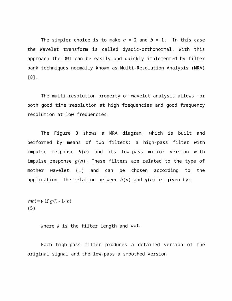
The simpler choice is to make a = 2 and b = 1. In this case the Wavelet transform is

called dyadic-orthonormal. With this approach the DWT can be easily and quickly implemented

by filter bank techniques normally known as Multi-Resolution Analysis (MRA) [8].

The multi-resolution property of wavelet analysis allows for both good time resolution

at high frequencies and good frequency resolution at low frequencies.

The Figure 3 shows a MRA diagram, which is built and performed by means of two

filters: a high-pass filter with impulse response h(n) and its low-pass mirror version with impulse

response g(n). These filters are related to the type of mother wavelet () and can be chosen

according to the application. The relation between h(n) and g(n) is given by:

( ) ( 1) ( 1 )nh n g K n (5)

where k is the filter length and .nZ

Each high-pass filter produces a detailed version of the original signal and the low-pass a

smoothed version.

The same Figure 3 summarizes several kinds of power systems application using MRA,

which has been published in the last decade [9]-[13]. The sampling rate (fs) showed in this

figure represents just only a typical value and can be modified according to the application with

the faster time-varying events requiring higher sampling rates.

It is important to notice that several of these applications have not been

comprehensively explored yet. This is the case of harmonic analysis, including sub-harmonic,

inter-harmonic and time-varying harmonic. And the reason for that is the difficulty to physically

understand and analytically express the nature of time-varying harmonic distortions from a

Fourier perspective. The other aspect, from the wavelet perspective, is that not all wavelet

mothers generate physically meaningful decomposition.

Another important consideration, mainly for protection applications is the

computational speed. The time of the algorithm is essentially a function of the phenomena (the

sort of information needed to be extracted), the sampling rate and processing time.

Applications which require detection of fast transients, like traveling waves [10][11], normally

have a very short time of processing. Another aspect to be considered is sampling rate and the

frequency response of the conventional CTs and VTs.

g

h

g

h

g

h

g

h

g

h

Fault identification

fs = 200 kHz

0 – 50 kHz

0 – 25 kHz 0 – 12,5 kHz

0 – fs/(2j+1 ) Hz

50 – 100 kHz

25 – 50 kHz 12,5 – 25 kHz

6,25 – 12,5 kHz

fs/(2j+1) – fs/(2j) Hz

fs = 100 kHz

fs = 50 kHz fs = 25 kHz

Surge capture

Detection of insipient failures

Fault location

Intelligent events records for power quality

Harmonic Analyses

..............

....

Figure 3 – Multi-Resolution Analysis and Applications in

Power Systems.

1.5 The Selection of the Mother Wavelet

Unlike the case of Fourier transform, there exists a large selection of wavelet families

depending on the choice of the mother wavelet. However, not all wavelet mothers are suitable

for assisting with the visualization of time-varying (harmonic) frequency components.

For example, the celebrated Daubechies wavelets (Figure 4a) are orthogonal and have

compact support, but they do not have a closed analytic form and the lowest-order families do

not have continuous derivatives everywhere. On the other hand, wavelets like modulated

Gaussian function or harmonic waveform are particularly useful for harmonic analysis due to its

smoothness. This is the case of Morlet and Meyer (Figure 4b) which are able to show amplitude

information [14].

Figure 4 – (a) Daubechies-5 and (b) Meyer wavelets.

The "optimal" choice of the wavelet basis will depend on the application. For discrete

computational the Meyer wavelet is a good option to visualization of time-varying frequency

components because the MRA can clearly indicate the oscillatory nature of time-varying

frequency components or harmonics in the Fourier sense of the word.

In order to exemplify such an application the MRA has been performed to decompose

and visualize a signal composed by 1 pu of 60 Hz, 0.3 pu of 7th harmonic, 0.12 pu of 13th

harmonic and some noise. The original signal has a sampling rate of 10 kHz and the harmonic

content has not been present all the time.

Figure 5 shows the results of a MRA in six level of decomposition, firstly using

Daubechies length 5 (Db5) and next the Meyer wavelet (dmey). It is clear that even a high

order wavelet (Db5 – 10 coefficients) the output signals will be distorted when using

Daubechies wavelet and, otherwise, will be perfect sinusoids with Meyer wavelet as it can be

seen at level 3 (13th ) and in level 4 (7th).

Some of the detail levels are not the concern because they result represent only noise and

transitions state.

Figure 5 – MRA with six level of decomposition using (a) Daubechies 5 wavelet and (b) Meyer wavelet.

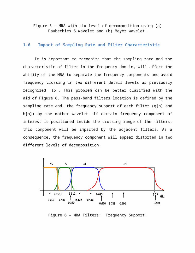
1.6 Impact of Sampling Rate and Filter Characteristic

It is important to recognize that the sampling rate and the characteristic of filter in the

frequency domain, will affect the ability of the MRA to separate the frequency components and

avoid frequency crossing in two different detail levels as previously recognized [15]. This

problem can be better clarified with the aid of Figure 6. The pass-band filters location is defined

by the sampling rate and, the frequency support of each filter (g[n] and h[n]) by the mother

wavelet. If certain frequency component of interest is positioned inside the crossing range of

the filters, this component will be impacted by the adjacent filters. As a consequence, the

frequency component will appear distorted in two different levels of decomposition.

1.250.6250.3120.156

d3d4d5a5

0.1800.300

0.420 0.5400.660 0.780 0.900

0.060kHz

1.260

1.250.6250.3120.156

d3d4d5a5

0.1800.300

0.420 0.5400.660 0.780 0.900

0.060kHz

1.260

Figure 6 – MRA Filters: Frequency Support.

In order to illustrate this question let us consider a 60 Hz signal in which a 5th harmonic

is present and whose sampling rate is 10 kHz. A MRA is performed with a ‘dmey’ filter.

According to the Figure 6 the 5th harmonic is located in the crossing between detail levels d4

and d5. The result can be seen in Figure 7 where the 5th harmonic appears as a beat frequency

in levels d4 and d5.

This problem previously cited may reduce the ability of the technique to track the

behavior of a particular frequency in time. However, artificial techniques can be used to

minimize this problem. For example, the simple algebraic sum of the two signals (d4+d5) will

result the 5th harmonic. Of course, if other components are present in the same level, a more

complex technique must be used.

As a matter of practicality the problem can be sometimes easily overcome as shown in

Figure 5 where the 5th and 7th harmonics (two of the most common components found in

power systems distortions) can be easily separated if an adequate sampling rate and number of

scales / detail coefficients are used.

Figure 7 – MRA with five decomposition levels. The 5th harmonic is revealed on level d4 and d5.

1.7 Time-Varying Waveform Distortions with Wavelets

Let us consider the same signal of the equation (2), whose variable amplitude of the 5th

harmonic is not revealed by Fourier transform. By performing the MRA with Mayer wavelet in

six decomposition levels the 5th harmonic has been revealed in d5 (fifth detailed level) during

all the time of analysis, including the correct amplitude of the contents.

As it can be seen from Figure 8 this decomposition can be very helpful to visualize time-

varying waveform distortions in which both frequency / magnitude (harmonics) and time

information is clearly seen. This can be very helpful for understanding the behavior of

distortions during transient phenomena as well as to be used for possible control and

protection action.

Figure 8 – MRA of the signal (equation (1)) showing time-varying 5th harmonic in level d5.

It is important to remark that other information such as rms value and phase can be

extract from the detailed and the approximation levels. For the previous example the rms value

during the interval from 0.2 to 2 s has been easily achieved.

1.8 Application to Shipboard Power Systems Time-Varying Distortions

In order to apply the concept a time-varying voltage waveform, resulting from a pulse in

a shipboard power system [16], is decomposed by MRA using a Meyer mother wavelet with five

levels (only detail levels 5 and 4 and the approximation coefficients are shown) is shown in

Figure 9. The approximation coefficient A5 shows the behavior of the fundamental frequency

whereas D5 and D4 show the time-varying behavior of the 5th and 7th harmonics respectively.

The time-varying behavior of the fundamental, 5th and 7th “harmonics” can be easily followed.

Figure 9 – Time-varying voltage waveform caused by pulsed load in a shipboard power system : MRA Decomposition using Meyer mother wavelet.

1.9 Conclusions

This chapter attempts to demonstrate the usefulness of wavelet MRA to visualize time-

varying waveform distortions and track independent frequency component variations. This

application of MRA can be used to further the understanding of time-varying waveform

distortions without losing the physical meaning of frequency components (harmonics) variation

with time. It is also possible that this approach could be used in control and protection

applications.

The chapter recognizes that the sampling rate / location of the filters for the successful

tracking of a particular frequency behavior, the significance of the wavelet mother type for the

meaningful information provided by the different detail levels decomposition, and the number

of detail levels.

A shipboard system simulation voltage output during a pulsed load application is then

used to verify the usefulness of the method. The MRA decomposition applying Meyer mother

wavelet is used and the transient behavior of the fundamental, 5 th and 7th harmonic clearly

visualized and properly tracked from the corresponding MRA.

1.10 References

[1] IEEE Task Force on Harmonics Modeling and Simulation: Modeling and Simulation of the

Propagation of Harmonics in Electric Power Networks – Part I: Concepts, Models and Simulation

Techniques, IEEE Trans. on Power Delivery, Vol. 11, No. 1, 1996, pp. 452-465

[2] Probabilistic Aspects Task Force of Harmonics Working Group (Y. Baghzouz Chair): Time-Varying

Harmonics: Part II Harmonic Summation and Propagation – IEEE Trans. on Power Delivery, No. 1,

January 2002, pp. 279-285

[3] R. E. Morrison, “Probabilistic Representation of Harmonic Currents in AC Traction Systems”, IEE

Proceedings, Vol. 131, Part B, No. 5, September 1984, pp. 181-189.

[4] P.F. Ribeiro; “A novel way for dealing with time-varying harmonic distortions: the concept of

evolutionary spectra” Power Engineering Society General Meeting, 2003, IEEE, Volume: 2 , 13-17

July 2003, Vol. 2, pp. 1153

[5] P. Flandrin, Time-Frequency/Time-Scale Analysis. London, U.K.: Academic, 1999.

[6] Newland D. E., ‘Harmonic Wavelet Analysis,’ Proc. R. Soc., London, A443, pp. 203-225, 1993.

[7] G. Matz and F. Hlawatsch, “Wigner Distributions (nearly) everywhere: Time-frequency Analysis of

Signals, Systems, Random Processes, Signal Spaces, and Frames,” Signal Process., vol. 83, no. 7,

2003, pp. 1355–1378.

[8] C. S. Burrus; R. A. Gopinath; H. Guo; Introduction to Wavelets and Wavelet Transforms - A Primer. 10

Ed. New Jersey: Prentice-Hall Inc., 1998.

[9] O. Chaari, M. Meunier, F. Brouaye. : Wavelets: A New Tool for the Resonant Grounded Power

Distribution Systems Relaying. IEEE Transaction on Power System Delivery, Vol. 11, No. 3, July

1996. pp. 1301 – 1038.

[10]F. H. Magnago; A. Abur; Fault Location Using Wavelets. IEEE Transactions on Power Delivery, New

York, v. 13, n. 4, October 1998, pp. 1475-1480.

[11]P. M. Silveira; R. Seara; H. H. Zürn; An Approach Using Wavelet Transform for Fault Type

Identification in Digital Relaying. In: IEEE PES Summer Meeting, June 1999, Edmonton, Canada.

Conference Proceedings. Edmonton, IEEE Press, 1999. pp. 937-942.

[12]V. L. Pham and K. P. Wong, Wavelet-transform-based Algorithm for Harmonic Analysis of Power

System Waveforms, IEE Proc. – Gener. Transm. Distrib., Vol. 146, No. 3, May 1999.

[13]O. A. S. Youssef; A wavelet-based technique for discrimination between faults and magnetizing

inrush currents in transformers,” IEEE Trans. Power Delivery, vol. 18, Jan. 2003, pp. 170–176.

[14]Norman C. F. Tse, Practical Application of Wavelet to Power Quality Analysis; CEng, MIEE, MHKIE,

City University of Hong Kong; 1-4244-0493-2/06/2006 IEEE.

[15]Math H.J. Bollen and Irene Y.H. Gu, “ Signal Processing of Power Quality Disturbances,” IEEE Press

2006.

[16]M. Steurer, S. Woodruff, M. Andrus, J. Langston, L. Qi, S. Suryanarayanan, and P.F. Ribeiro,

Investigating the Impact of Pulsed Power Charging Demands on Shipboard Power Quality , The

IEEE Electric Ship, Technologies Symposium (ESTS 2007) will be held from May 21 to May 23, 2007

at the Hyatt Regency Crystal City, Arlington, Virginia, USA.

Chapter 2 - Wavelets for the Measurement of Electrical Energy

Signals

Johan Driesen

2.1 Introduction

In modern electrical energy systems, voltages and especially currents become very

irregular due to the large numbers of non-linear loads and generators in the grid. More in

particular, power electronic based systems such as adjustable speed drives, power supplies for

IT-equipment and high efficiency lighting and inverters in systems generating electricity from

distributed renewable energy sources are as many sources of disturbances. Distortions

encountered are for instance harmonics, rapid amplitude variations (flicker) and transients, all

being elements of ‘power quality’ problems.

In this situation, the registration of electrical energy signals and power related quantities

may become problematic, due to differences in power definitions, extended for non-

fundamental frequency content, non-standardized measurement procedures, all based on

sinusoidal voltages and currents, and equipment originally designed for undistorted signals [1].

In general, voltage and current signals have become less stationary and periodicity is

sometimes completely lost. This fact poses a problem for the correct application of Fourier-

based frequency domain power quantities. Practical measurements use the FFT-algorithm for

this purpose, implicitly assuming infinite periodicity of the signal to be transformed. Therefore,

the registered power quantities are often unreliable and it is not possible to localize distortions

with a higher resolution than the time slot.

2.2 Real Wavelet-Based Power Measurement Approaches

2.2.1 Basic principles

A wavelet transform maps the time-domain signals of voltage(s) and current(s) in a real-

valued time-frequency domain (using a notation similar to[2]), where the signals are described

by the wavelet coefficients:

(1)

(2)

with

and

(3)

and

(4)

(j: wavelet frequency scales, k: wavelet time scale, c and d: wavelet coefficients – the

accent indicates the voltage coefficients).

2.2.2 Active power

The active power is computed as an averaged sum of the physical power transfer over a

certain time interval (T: averaging time interval and N the highest scale):

(5)

In this way it is possible to distinguish the power over the different wavelet scales, to be

interpreted as frequency bands. Most interest usually goes to the base band j0 containing the

fundamental power frequency coefficients.

2.2.3 Reactive Power

Reactive power is computed in a similar way, but the voltage signal first has to pass a

phase shifting filter network, producing a delay or phase shift of 90° in the approach of [3].

(6)

For purely sinusoidal voltages and currents, this results in a correct value, but in the

presence of distortions it is just one of possible definitions of reactive power, still being a topic

of discussion. In the phase shifting implementation approach for reactive powers, often used in

traditional measuring equipment, only the ‘baseband’ value Qj0 is associated to the accepted

fundamental reactive power [4].

The implementation of the 90°-phase shift, actually a time delay, in the time-frequency

domain, after the wavelet transform instead of in the time domain as in (6), forms an

interesting, yet simple alternative for a shift in the time domain. Such a delay in the wavelet

domain means a shift of the time-bound wavelet coefficient as calculated in (4). Since there are

far less coefficients involved than time samples, this comes down to a rather simple memory

operation.

Hence, no special filter is required, considerably simplifying the computation procedure.

Only an extra vector of memory elements to store the previous wavelet coefficients is required.

The shift M of the coefficients depends on the wavelet transform parameters, more in

particular the number of coefficients describing a fundamental period in the base band:

(7)

with the double accent indicating the delayed coefficients, here the voltage coefficients.

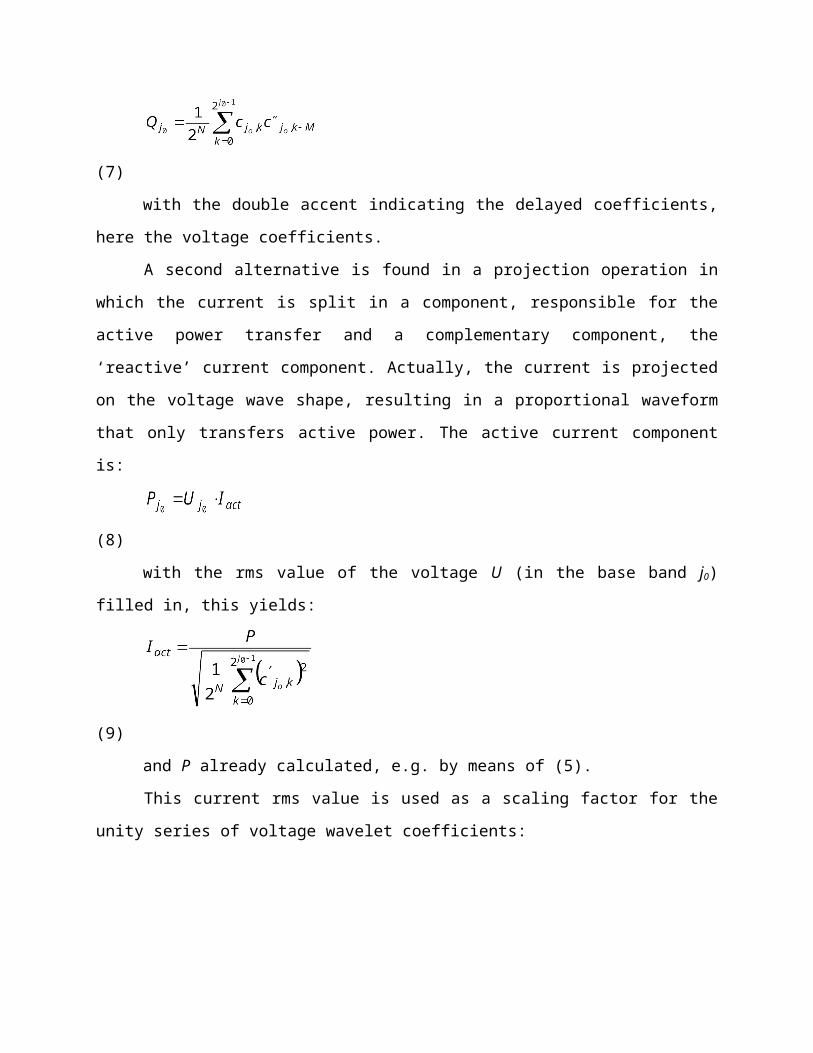
A second alternative is found in a projection operation in which the current is split in a

component, responsible for the active power transfer and a complementary component, the

‘reactive’ current component. Actually, the current is projected on the voltage wave shape,

resulting in a proportional waveform that only transfers active power. The active current

component is:

(8)

with the rms value of the voltage U (in the base band j0) filled in, this yields:

(9)

and P already calculated, e.g. by means of (5).

This current rms value is used as a scaling factor for the unity series of voltage wavelet

coefficients:

(10)

Hence, the wavelet transform coefficients of the current proportional to the voltage

(also in the time domain), transmitting the same active power, are obtained.

The current split is obtained for the base band in the time-frequency domain by

computing the complementary ‘reactive’ series of wavelet coefficients:

(11)

In this way, the rms value of the reactive current component can be defined.

(12)

This is then used to compute the reactive power value:

(13)

2.3 Application of Real Wavelet Methods

As an example, the two approaches mentioned above are applied on a voltage and

current containing harmonic distortion, mainly fifth order harmonics (Figure 3).

Voltage Current

Figure 3. Voltage and current period used for the example calculation.

These waveforms are sampled at 128 samples per period and are wavelet transformed

using a ‘symmlet’ wavelet [5]. Both resulting coefficients are plotted in Figure.

Wavelet coefficients of voltage Wavelet coefficients of current

Figure 4. Wavelet coefficients at different scales. Top scale is associated with the base band.

Note that the base band is described by only four coefficients. Hence buffering in order

to obtain the 90° shift represents a limited operation, compared to a delay or phase shift in the

time domain in which all 128 samples have to be processed.

The active and reactive powers are calculated and compared to analytically derived

reference quantities in Table 1.

Table 1. Comparison of computed power quantities.

P Q

Analytical reference 995.93 575.00

Delay approach 991.80 575.24

Splitting approach 991.80 575.24

It can be noticed that the accuracy of the wavelet approach is rather good: the

processed values are within 0.5 % of the analytical values. The difference is due to numerical

errors and ‘leakage’ between frequency bands.

2.4 Concept Using Complex Wavelet Based Power Definitions

2.4.1 Introduction

The power calculation procedure using real wavelets is less subject to errors due to the

irregularity of signals, but is still based on classical averaging over a designated time interval (5),

an idea also present in the derivation of regular frequency domain quantities, where a sampled

interval is covered. Complex wavelets seem only to have rarely been used in power system

analysis, except for [6].

To be able to calculate any power quantities, one needs to be able to analyze

amplitudes and phase differences between the related voltage(s) and current(s). A (complex)

Fourier transform yields the appropriate phasors, but a (real) wavelet transformed signal does

not readily deliver phase information. The ‘hidden’ phase-related information, present in the

time localization property of the wavelet coefficient, influences the average power values as in

[2], [3].

A complex wavelet, however, does yield phase information. It is even possible to

retrieve an instantaneous phase (t) using the polar representation of the complex coefficients

[5]. It is therefore a candidate to serve as a basis in novel power definitions having better time

localization properties. Therefore, this would result in true time-frequency domain power

quantities.

2.4.2 Complex wavelet based power definitions

The relevant voltages and currents are transformed to the time-frequency domain using

a well-chosen complex wavelet (t), with scaling parameter s (setting the frequency range) and

translation parameter t (determining the time localization) [5]:

(14)

In a single-phase system this yields two series of complex wavelet coefficients for the

voltage U and for the current I, indicated by a subscript W: UW and IW. From these coefficients,

instantaneous amplitude and phase values are derived for the different subbands.

(15)

(16)

For most power measurement applications, the most interesting subband is the one

covering the fundamental frequency, here indicated as sf. A complex-wavelet based power

quantity is then defined in a way analogous to the Fourier-based active power definition, now

using the instantaneous voltage and current amplitude and the instantaneous phase difference

between voltage and current:

(17)

with the phase difference, based on the difference of the instantaneous phases:

(18)

Similarly, a complex wavelet based reactive power quantity can be defined as well:

(19)

Both pW and qW can be obtained immediately by

(20)

A ‘momentary’ power factor can be defined using the instantaneous phases.

(21)

An apparent power-like is quantity is obtained as well:

(22)

2.4.3 Wavelet choice

The complex wavelet (14), has to be appropriate for the analysis of power signals.

Therefore, a smooth oscillating function is preferred. The following functions are candidate [5]:

the complex Gaussian wavelet (Cp is a scaling parameter):

(23)

and the complex Morlet wavelet (fb: a bandwidth parameter, fc: the center frequency):

(24)

The real and imaginary part of this wavelet, with fb=50 Hz are plotted in Figure.

real part imaginary part

Figure 5. Real and imaginary part of the Morlet wavelet.

2.4.4 Discussion: Physical interpretation

The physical interpretation of power definitions is always debatable. The only physically

correct value is the time domain based power p(t)=u(t)i(t), containing a DC part as well as

higher frequency oscillations. Its average, global or for a certain harmonic frequency, in case of

periodic signals, is expressed by the frequency domain active powers P or Ph [4]. Reactive power

can be regarded in a similar way, as a measure for the power oscillating between source and

user.

The complex wavelet based power rather yields a sort of sliding average power, as the

time window over which it averages is limited to the length of the wavelet function and

determined by the dilation parameter [5]. Due to the decaying shape of the wavelet, this

average is weighted. Thus, this power can be localized in time. The frequency localization is

broader than just a sharp single harmonic as the complex wavelet covers a certain frequency

band.

2.4.5 Comparison with Fourier based approach

A traditional Fourier-based power computation starts with calculating an FFT of a frame

of current or voltage samples. Then, adequate frequencies are selected and processed, yielding

one value per power quantity over the whole frame, resulting in a poor time resolution.

Alternatively, to provide a better time resolution, one can use overlapping frames, causing one

sample to be used more than once. The frequency resolution is equidistant.

A wavelet transform is typically calculated using filters [5]. This yields several

transformed coefficients over the same time frame, depending on the scaling of the wavelet

basis. This allows to provide a better time localization. In return, the frequency resolution is not

as sharp, especially not for the higher frequencies. This poses not so much problems in practical

power systems as one is mainly interested in a sharp distinction of the fundamental frequency

behavior, a relatively good distinction of the low-frequency harmonics, which in practice are

found in pairs (e.g. 5th/7th) and a rough idea about high-frequency phenomena. The typical

wavelet frequency resolution pattern is well-suited for such requirements.

2.5 Examples

2.5.1 Practical implementation aspects

The wavelet function providing the best results, in the sense that similar results for

stationary signals were obtained as with Fourier analysis, was the Morlet function (24), with a

pseudo-frequency of 50 Hz, the fundamental power system frequency in the examples

(fb=4.10-4, fc=50 Hz). This wavelet function is limited to 8 periods of the fundamental frequency.

One period contains 128 samples.

In the following examples, the (continuous) wavelet transform is implemented as a

convolution. In a practical implementation a faster filter algorithm is required. To get rid of

boundary effects, an appropriate number of transformed samples is omitted.

Example 1: voltage dip

The first example shows a typical non-periodic distortion, a dip in the voltage (Figure).

This power quality problem may occur due to sudden change in the load, e.g. the start of a large motor or an arc

furnace. In an FFT, this results in the presence of subharmonic frequencies and a lower fundamental, without

knowing when the dip occurred. The current is identical to the current in the previous example.

Figure 6. Voltage with a dip and current with harmonics.

The resulting powers pW and qW are computed and plotted in Figure. They clearly show the

sudden drop in transferred power and change in reactive power due to the local change in phase difference. The

small overshoots at the beginning of the power curves are due to the discontinuous jump in phase angles in this

simulated voltage. These will be smaller in reality as most voltage dips settle in more slowly. Even more, the

reaction of the load, usually a lower current, is not taken into account.

Figure 7. pW and qW associated to the waveforms in Figure.

Example 2: dynamically changing current

The second example contains a continuously rising distorted current, for instance due to an adjustable speed

drive with an increasing mechanical output, for instance due to increasing speed.

Figure 8. Clean voltage and transient harmonically distorted current.

The resulting powers pW and qW are computed and plotted in Figure. They follow the smooth

rate of change of the current.

Figure 9. pW and qW associated to the waveforms in Figure.

In a Fourier based analysis, the spectrum of this non-periodic current would result again in

some sort of subharmonic occurrences.

2.6 References

[1] J. Driesen, T. Van Craenenbroek, D. Van Dommelen, “The registration of harmonic power by

analog and digital power meters,” IEEE Trans. on Instrumentation and Measurement, Vol.

47, No. 1, February 1998, pp. 195-198.

[2] W.-K. Yoon, M.J. Devaney, “Power Measurement Using the Wavelet Transform,” IEEE Trans.

on Instrumentation and Measurement, Vol. 47, No. 5, October 1998, pp. 1205-1210.

[3] W.-K. Yoon, M.J. Devaney, “Reactive Power Measurement Using the Wavelet Transform,”

IEEE Trans. on Instrumentation and Measurement, Vol. 49, No. 2, April 2000, pp. 246-252.

[4] IEEE Working Group on Nonsinusoidal Situations: Effects on Meter Performance and

Definitions of Power, “Practical Definitions for Powers in Systems with Nonsinusoidal

Waveforms and Unbalanced Loads: A Discussion,” IEEE Trans. on Power Delivery, Vol. 11,

No. 1, January 1996, pp. 79-101.

[5] S. Mallat, A Wavelet Tour of Signal Processing, Academic Press, 1999.

[6] M. Meunier, F. Brouaye, “Fourier transform, Wavelets, Prony analysis: Tools for Harmonics

and Quality of Power,” Proc. 8th Int. Conf. On Harmonics and Quality of Power (ICHQP’98),

Athens, Greece, 14-16 October 1998, pp. 71-76.

Chapter 3 – A Conceptual Fuzzy Logic Application for Diagnosis of Time-

Varying Harmonics in Power SystemsBryan R. Klingenberg, Paulo F. Ribeiro, Siddharth Suryanarayanan

3.1 - Introduction

Harmonic distortion in power systems continues to grow in importance due to the

proliferation of non-linear loads and sensitive electronic devices. Due to the inherently time-

varying nature of harmonics, it is difficult to predict the exact level of harmonics in the system.

The use of traditional tools such a fast Fourier transforms (FFT) may not be appropriate for the

analysis of time-varying harmonics. Hence, more advanced techniques are required to properly

quantify their impact. This chapter proposes the utilization of fuzzy logic to analyze, compare,

and diagnose time-varying harmonic distortion indices in a power system.

When non-linear loads are connected to an electric power system they tend to draw

non-linear currents and consequently distort the system voltage [1]. Typically the harmonics

are assumed to be periodical/time-invariant. However harmonic components are continually

changing with time [2]. It is important then to look at the harmonics from a time-varying

perspective. Harmonic distortions can adversely affect many systems by causing erratic

behavior in microcontrollers, breakers, and relays. The most substantial effect of harmonic

distortions within a system is the increase in the temperature which results in increased losses,

transformer derating, and possible equipment failure [1], [2]. When techniques such as FFT are

applied to quantify the spectrum of time-varying harmonics, the method suffers a break down.

Hence, in order to analyze, compare, and quantify time-varying nature of harmonic distortions,

the framework of a conceptual application of a fuzzy logic technique is presented in this

chapter. Synthetic data is used for the purpose of demonstrating the concept.

3.2 Fuzzy Logic

In a traditional bivalent logic system an object either is or is not a member of a set. The

idea of fuzzy sets is that the members are not restricted to true or false definitions. A member

in a fuzzy set has a degree of membership to the set. For example, the set of temperature

values can be classified using a bivalent set as either hot or not hot. This would require some

cut-off value where any temperature greater than that cut-off value is ‘hot’ and any

temperature less than that value is ‘not hot’. If the cut off point is at 50oC then this set does not

differentiate between a temperature that is 20oC and a temperature of 49oC. They are both

‘not hot’ [3], [4] and [5].

If a fuzzy set were to be used in this situation each member of the set, or each

temperature, would have a degree of membership to the set of temperature. The function that

determines this degree of membership is called the fuzzy membership function as shown in

Figure.

Figure 10: Fuzzy membership function for hotness

There are different membership function topologies that can be used; the most

common are triangular, gaussian and sigmoidal. The function in Figure is a sigmoidal function.

The attributes of the membership function can be modified based on the desired input [6]. If

the relevant temperature range was between 20 and 60 degrees, for example, and more weight

was needed for higher temperatures then an appropriate membership function can be

determined. The determination of this function is dependant on the desired weighting of the

input.

3.3 Fuzzy Logic Control

The basic fuzzy logic control system is composed of a set of input membership functions,

a rule-based controller, and a defuzzification process. The fuzzy logic input uses member

functions to determine the fuzzy value of the input. There can be any number of inputs to a

fuzzy system and each one of these inputs can have several membership functions. The set of

membership functions for each input can be manipulated to add weight to different inputs.

The output also has a set of membership functions. These membership functions define the

possible responses and outputs of the system [6].

The fuzzy inference engine is the heart of the fuzzy logic control system. It is a rule

based controller that uses If-Then statements to relate the input to the desired output [6]. The

fuzzy inputs are combined based on these rules and the degree of membership in each function

set. The output membership functions are then manipulated based on the controller for each

rule. Several different rules will usually be used since the inputs will usually be in more than

one membership function. All of the output member functions are then combined into one

aggregate topology. The defuzzifaction process then chooses the desired finite output from

this aggregate fuzzy set. There are several ways to do this such as weighted averages,

centroids, or bisectors. This produces the desired result for the output.

3.4 Fuzzy Logic in Power Systems

There are relatively few implemented systems using fuzzy logic in the power industry at

this time [4]. This is due to the fact that most of the focus with fuzzy systems has been in

research and not in implementation. The application of fuzzy logic in power systems has been

mainly focused on controllers and system stabilizers [5]. There are other applications in areas

such as prediction, optimization and diagnostics [5]. The diagnosis area of application is

particularly attractive because it is difficult to develop precise numerical models for failure

modes [4]. Understanding failure modes of a system is usually only done by approximations at

best, therefore, the diagnosis of a failure is then difficult to do because of the inherent

imprecision. There is rarely a single measurement that can indicate impeding failure and so

several measurements need to be taken and compared based on the specific system [5]. A

generic diagnostic tool is difficult to develop since it needs to be tuned to a specific system to

obtain reasonable performance [4].

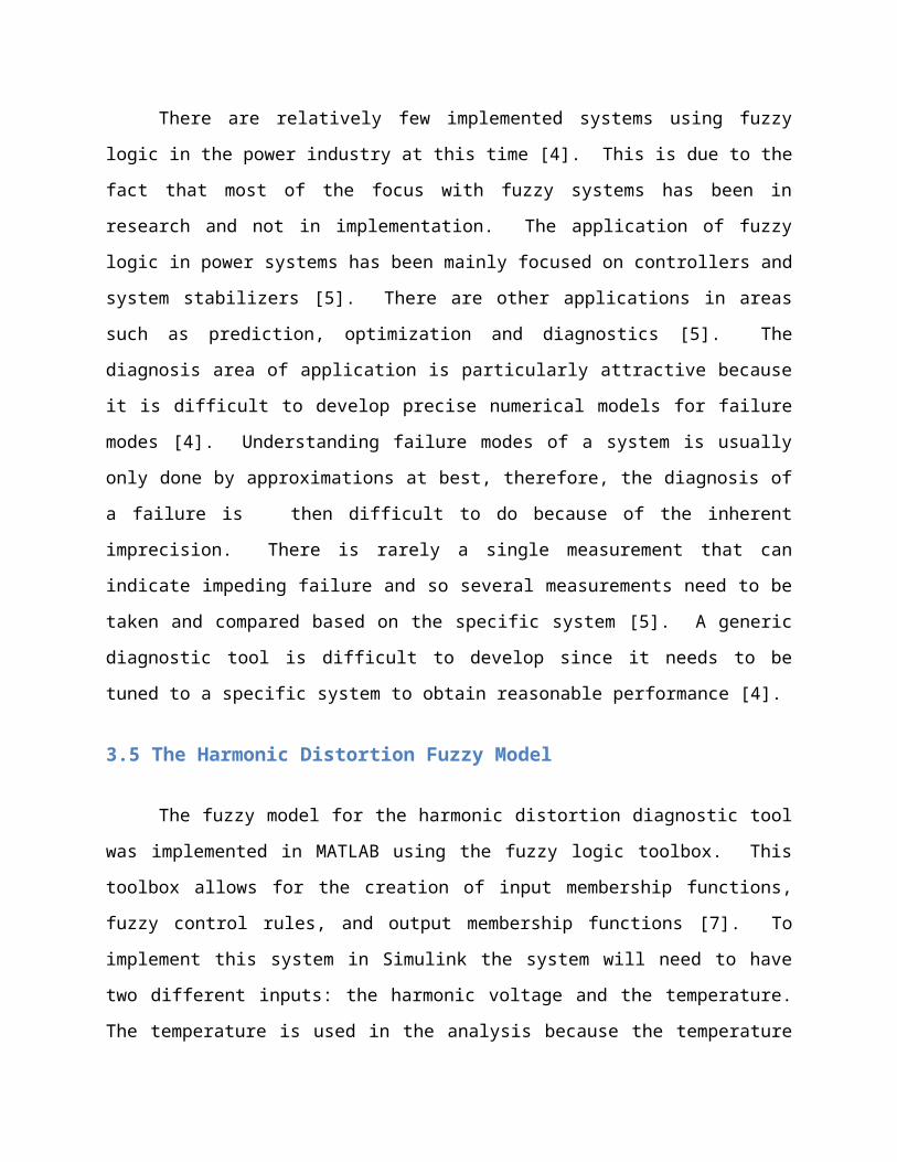
3.5 The Harmonic Distortion Fuzzy Model

The fuzzy model for the harmonic distortion diagnostic tool was implemented in

MATLAB using the fuzzy logic toolbox. This toolbox allows for the creation of input membership

functions, fuzzy control rules, and output membership functions [7]. To implement this system

in Simulink the system will need to have two different inputs: the harmonic voltage and the

temperature. The temperature is used in the analysis because the temperature of a piece of

electrical equipment will increase as the harmonic distortion content increases [2]. These two

inputs will then be processed by a fuzzy logic controller that will output a degree of caution.

This degree of caution is then decoded into one of four possible outputs: No problem, Caution,

Possible Problem, and Imminent Problem. A simple (two-variable example) diagnostic system

was created as shown in Figure .

Figure 11: Harmonic Distortion Diagnostic Simulink Model

This diagnostic system uses random number inputs for the harmonic voltage and

temperature inputs. The harmonic voltage input (shown in Figure) is a random distribution in

the range of 0 to 10. The temperature input (shown in Figure) is a random distribution in the

range of 30 to 100 degrees Celsius.

Figure 12: Harmonic Voltage Input

These input function ranges can now be used in determining the fuzzy membership sets.

The fuzzy system will have these two inputs and one indicating output as shown in Figure. The

fuzzy system used will be a mamdani system [6], and the centroid method for defuzzification

[6]. The input membership function for harmonic voltage (shown in Figure) will have five

membership functions: very low, low, medium, high, and very high. The range of this function

is 0 to 10, these are the possible input values. The very low and very high membership

functions continue on to infinity in either direction to include any voltage value out of range.

Figure 13: System Temperature Input

Figure 14: The Fuzzy Logic Diagnostic Controller

Figure 15: The Harmonic Voltage Input Membership Functions

The harmonic voltage membership functions define anything from 0 to 5 as low, using a

triangular function. Anything from 2.5 to 7.5 is medium, and anything from 5 to 10 is high. An

input with a harmonic voltage of 3 will have about an 80% membership in the low function and

about a 20% membership in the medium function. The total membership in this case will add

up to be 100% but this is not required in a fuzzy set.

Figure 16: The System Temperature Input Membership Functions

There are four temperature input membership functions as shown Figure. The below

normal function is a triangular function centered at 30 that extends up to 53 degrees. The

normal triangular function is centered at 53 degrees, extending from 30 to 76 degrees at its

limits. The over heating triangular membership function is centered at 76 degrees with the

same magnitude of range as the normal function. The very hot function begins at 76 degrees

and peaks at 100 where it extends on past the set max input of 100 to cover out of limit values.

The output has four membership functions, no problem, caution, possible problem, and

imminent problem (shown in Figure). These membership functions are all triangular and are

spread evenly on a range of 0 to 1.

Figure 17: The Output Membership Function

Once all of the input and output membership functions have been defined the heart of

the control can now be defined; the rules. The fuzzy rules are in the form of if-then statements.

These statements look at both inputs and determine the desired output. In this system

increasing voltage and increasing temperature will lead to an imminent problem. A low

temperature with a relatively high voltage will not necessarily be an imminent problem though.

The rules defined for this system are in listed in Table 2.

Table 2: MEMBERSHIP RULES

If Harmonic Voltage is:

And the temperature

is:

Then the Output is:

very_low below_normal no_problem

very_low normal no_problem

very_low over_heating no_problem

very_low very_hot Caution

low below_normal no_problem

low normal no_problem

low over_heating Caution

low very_hot Possible_problems

medium below_normal no_problem

medium normal Caution

medium over_heating Possible_problems

medium very_hot Possible_problems

high below_normal Caution

high normal Possible_problems

high over_heating Possible_problems

high very_hot Imminent_problems

very_high below_normal Possible_problems

very_high normal Possible_problems

very_high over_heating Imminent_problems

very_high very_hot Imminent_problems

These rules are the defining elements of this system. They determine the output based

on the input. These rules can be looked at graphically as a rule map (shown in Figure). This rule

map illustrates the response of the system to different inputs. On the map the dark blue

represents no problem and the light yellow represents an imminent problem. The intermediate

colors show the mix of fuzzy options in between.

Figure 18: Fuzzy Control Rule Map

Now that the fuzzy control system has been entirely defined it is exported into the

Simulink model. The model includes some decoding logic that will output different discrete

levels for each of the possible outputs similar to the one shown in Figure . This could serve as

input to some other system.

3.6 Expanded Model

The inputs for this example system have been shown before; they are randomly

generated data within a valid range. The system can be simulated using this data. There are

four different output scopes that will indicate the output signal of the fuzzy controller. These

results could be then used to compute probability distribution functions and or send alarm

notes to a central controller.

A better diagnostic tool can be developed that takes more data into account and

provides a single output [5]. This can be done using the previous model and setting up a more

involved case. This case will look at the fundamental voltage variation as well as the variation

of the third, fifth and seventh harmonics. The following variations, shown in Table 3, will be

used in this case.

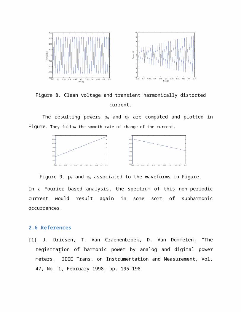
Table 3: INPUT VARIATIONS

Fundamental +/- 10%

V3 1% – 8%

V5 1% – 8%

V7 1% – 8%

VTHD 1% – 13%

Temperature 30°C – 100°C

These inputs were chosen based on the recommended harmonic voltage limits from [1].

The Fundamental and the harmonics will have uniform random function generators as inputs.

These function generators will generate a uniform distribution of inputs within the variances

given in Table 3. The total harmonic distortion will be calculated depending on these inputs

and so it will be in the range of 1% to 13%, these are the best and worst case scenarios. The

temperature variation will remain the same as in the previous case.

Using this input data and the basic model developed in the first case a Simulink model can be

developed that processes all the input data and gives an appropriate indication for each

harmonic, the fundamental, and THD. These indications will remain the same as in the previous

case. Each indicator will have a fuzzy logic controller that implements one of three control

topologies, one for the fundamental, THD, and the harmonics. The final model can be seen in

Figure.

Figure 19: Final Simulink Model

The first fuzzy logic controller will use the fuzzy inference system that has a rule similar

to the one shown in Figure except that the scale is now from 0.9 to 1.1. This represents the

percentage of the ideal. The total harmonic distortion rule surface and the harmonic voltage

rule surfaces will be essentially the same except with different scales again based on the

variations given in Table 3. The second fuzzy controller in Figure uses the THD fuzzy inference

system and the remaining three fuzzy controllers use the harmonic fuzzy inference system.

The S-functions in the model are simple MATLAB files that process the fuzzy logic

controller output and determine the output level using the code shown in Figure.

Figure 20: S-function Code

This code will split the fuzzy output into four ranges and then output either a 0,1,2, or 3

corresponding to No Problem, Caution, Possible Problems, and Imminent Problems. This

provides a simple way to visualize the output data for this proof of concept case. After this final

decoding step the output is sent to scopes and also to workspace variables. These workspace

variables will allow for statistical analysis after simulation and eliminate the need for having

four separate scopes for each fuzzy controller.

3.7 Simulation Results

The inputs for the simulation are all from uniform random number generators that will

generate random numbers within the previously defined ranges. The system will be modeled

for a 24 hour period with the number generators producing a new number every 2 minutes.

This is what the input from a typical power system monitoring device would be [1].

Each random number generator has a different seed value to produce a different set of

numbers. All of the inputs can be seen in Figure. From top to bottom the inputs are the

fundamental, third harmonic, fifth harmonic, seventh harmonic and the temperature in

percentages. The data used in this system is purely fictitious since this is a proof of concept

experiment. This model provides a base for future applications which would use real data. In

any future application the system would have to be retuned to meet the requirements of that

system. This retuning process would involve the membership functions and the fuzzy rules and

is a common aspect of fuzzy logic applications [5].

The outputs of the system will be one of four options, 0,1,2, or 3 which represent the

possible warning indicators. These outputs can be seen in Figure. In that figure the outputs,

from top to bottom, are the fundamental, third, fifth, seventh harmonics, and finally the total

harmonic distortion.

Figure 21: All System Inputs (top down): Fundamental, Third, Fifth, Seventh Harmonics and

Temperature

Figure 22: Output Indicators (Top down): Fundamental, Third, Fifth, Seventh Harmonics and

THD

Most of the outputs appear to be in the Caution or Possible Problems state by looking at

the output plot. The outputs were exported into MATLAB where they could be plotted in a

histogram to so that the distribution of outputs could be easily seen. This histogram can be

seen in Figure. From this we can tell that most of the results are the first three states, except

with the total harmonic distortion where most of the results are either Caution or Imminent

Problems.

Figure 23: Output Histogram: Uniform Distribution

The simulation was repeated with different input distributions as well. Figure shows the

output histogram when the inputs are all Gaussian distributions. The output histograms are

broken up into four sections as a result of the filtering that occurs in the S-function code, shown

in Figure, which reduces the fuzzy controller output to only four states.

Figure 24: Output Histogram: Gaussian Distribution

The output distribution of the fuzzy controllers can be plotted with higher resolution, for

an example the output of the fundamental fuzzy controller can be seen in Figure. That output

is the unprocessed output of the fuzzy logic controller.

Figure 25: Fundamental Fuzzy Logic Controller Output Histogram

The simulation is based on possible typical data modeled by random number

generators. Any statistical trends in the system are a result of the nature of the input for this

simulation. The inputs for this simulation do not represent actual harmonic levels and so the

statistical analysis is performed simply to show how it would be done if real data inputs were

used. Other parameters such as voltage unbalance and mechanical vibration may be studied as

outputs as shown in Figure.

Harmonic Distortion

Voltage Unbalance

Mechanical Vibration

Equipment Temperature

Fuzzy Logic Diagnostics

Harmonic Distortion

Voltage Unbalance

Mechanical Vibration

Equipment Temperature

Fuzzy Logic Diagnostics

Figure 26. Schematic of an expanded fuzzy logic based diagnosis tool

3.8 Conclusions

This chapter presented a methodology to analyze harmonic distortion impact on system

equipment using a fuzzy logic based system. The examples simulated indicate the potential for

using such a procedure for studying complex systems and performing a meaningful evaluation

and/or analysis of the impact of time-varying harmonic distortion on a power system. The use

of advanced techniques such as fuzzy logic may help in overcoming the challenges faced with

traditional tools such as FFT for the diagnosis and analysis of time-varying harmonics. Other

intelligent techniques such as agents and artificial neural networks may serve as suitable

candidates for the analysis and diagnosis of time-varying harmonic distortions.

3.9 References

[1] IEEE Std 519-1992, IEEE Recommended Practices and Requirements for Harmonic Control in

Electrical Power Systems.

[2] Halpin S.M., “Harmonics in Power Systems”, in The Electric Power Engineering Handbook,

L.L. Grigsby, Ed. Boca Raton: CRC Press, 2001.

[3] Kosko, Bart. Fuzzy Thinking. New York: Hyperion, 1993.

[4] T. Hiyama and K. Tomsovic, "Current Status of Fuzzy System Applications in Power Systems,"

Proceedings of the IEEE SMC99, Tokyo, Japan, October, 1999, pp. VI 527-532.

[5] K. Tomsovic, "Fuzzy Systems Applications to Power Systems," Chapter IV-Short Course, The

1999 International Conference on Intelligent System Application to Power Systems, Rio de

Janeiro, Brazil, April 1999.

[6] Nguyen, Hung T., Nadipuram R. Prasad, Carol L. Walker, and Elbert A. Walker. A First Course

in Fuzzy and Neural Control. Boca Raton, FL: Chapman & Hall/CRC, 2003.

[7] The MathWorks. [Online]. Fuzzy Logic Toolbox. Available:

http://www.mathworks.com/products/fuzzylogic/ [Dec 16, 2005]

Chapter 4 - Real Time Simulation for Time-Varying Harmonic Distortion

Analysis: A Novel Approach

Y. Liu, and P. Ribeiro

4.1 - Introduction

A novel approach to time-varying harmonic distortion assessement based on real-time

(RT) hardware-in-the–loop (HIL) simulation is proposed. The sensitivity for power quality

deviations of a variable speed drive controller card was tested in the platform. The successful

experiment has contributed to the conceptive design of a universal power quality test bed,

which would have the function of testing the immunity of electric components and equipment

and the consequent impact on AC distribution systems.

Electromagnetic transient simulations or laboratory experiments are often used for

power quality studies. The results of different simulation programs could be different because

of the usage of different mathematic models. Also, the simulation results largely depend on the

accuracy and complexity of those models. On the other hand, the disadvantages of the

laboratory experiments are the high cost and the large amount of developing time. Also, the

power quality impact on power systems is hardly achieved due to the difficulties of connecting

a tested device to real power systems. To achieve better accuracy on the power quality studies

of large and complex power systems in an economic way, a novel power quality assessment

method based on a real time (RT) hardware-in-the-loop (HIL) simulator is proposed. Hardware-

in-the-loop is an idea of simultaneous use of simulation and real equipment. Generally, a HIL

simulator is composed of a digital simulator, one or more hardware pieces under test, and their

analog and digital signal interfaces (e.g., high performance A/D and D/A cards).

4.2 Description of the RT-HIL Platform

A RT-HIL platform is currently being established at the Center for Advanced Power

Systems (CAPS) at Florida State University, Tallahassee, Florida. The platform has been designed

for research on NAVY all-electric ship power systems. Fig. 1 shows the diagram of the RT-HIL

platform. The platform is composed of a digital simulator (RTDSTM), tested hardware, and their

interface (e.g., power amplifiers and transducers). The simulator can be used either as an

independent simulation system (e.g., no hardware in the loop), or with tested hardware. In Fig.

1, a real power electronic device is connected to the simulated power system through D/A

adaptors and power amplifiers. The supply current of the AC/DC converter is measured and fed

back into the system at the common coupling point through transducers and A/D adaptors. In

fact, any component (e.g., controllers of power electronic devices, and control and protection

equipment) in power systems could be tested in the platform.

Fig. 1. Diagram of the RT-HIL platform at the CAPS, Tallahassee, FL

The distribution system of the US coast guard icebreaker “Healy” has been simulated in

real-time to demonstrate the simulator’s capabilities. Fig. 2 shows a good agreement between

the complete software simulation results and the field measurements taken during Healy’s

commissioning trials in 1998.

22:13:12.640 22:13:12.645 22:13:12.650 22:13:12.655 22:13:12.660-200

-150

-100

-50

0

50

100

150

200

22:13:12.640 22:13:12.645 22:13:12.650 22:13:12.655 22:13:12.66022:13:12.640 22:13:12.645 22:13:12.650 22:13:12.655 22:13:12.660-200

-150

-100

-50

0

50

100

150

200

-200

-150

-100

-50

0

50

100

150

200

Measuredwaveformevent at05/13/00 22:13:12.64

HV Bus PT output voltage [V]

t [h:m:s]

Simulatedwaveform dt = 65 s

Phase A

Phase B

Phase C

Fig. 2. Measured AC bus voltage waveforms (broken gray lines) of US Coast Guard icebreaker (all four cycloconverter bridges operating) compared to the simulated waveforms (solid colored) using the digital simulator model (only one bridge of each of both cycloconverter drives operating) Error: Reference source not found].

4.3 Sample Case: Testing the Sensitivity of a Thyristor Firing Board to Poor Quality Power

An Enerpro FCOG 6100 three-phase thyristor firing board was tested in the platform for

its sensitivity to poor quality power. Also, the impact of its sensitivity on the DC load and the AC

distribution systems is considered. The schematic of the simulated AC distribution system is

shown in .

EMBED Visio.Drawing.6

Fig. 3. Diagram of the simulated industrial distribution system and rectifier load (60 Hz, power base = 833 kW)

To consider the application of the board on NAVY all-electric-ships, extreme

conditions (e.g., significant frequency change) are simulated in the test. Table 4 shows the RT-

HIL simulation results.

Table 4 The RT-HIL simulation results for the firing board

PQ phenomena Simulation results

THD Tolerate THD up to 14.8% and higher

Tolerance has no impact on distribution systems

Voltage sag

Tolerance depends on not only the time duration and

voltage reduction, but also phase shift

Tolerance results in DC voltage drop or blackout

Frequency change Tolerate system frequency from 30 Hz to 80 Hz

Fig. 4 and Fig. 5 show the single-phase voltage sag with and without any phase shift and

their impact on the DC output voltage of the rectifier. The sag with a phase shift resulted in the

reboot of the firing board. The reboot then resulted a 0.1 s DC blackout and about 1.5 s

transient process on both DC and AC systems. However, the sag without phase shifts only

resulted in a DC voltage drop. This finding can not be discovered by using traditional laboratory

tests (e.g., changing the amplitude of one phase voltage in a 3-phase vari AC).

Fig. 4. Single-phase voltage sag (0.1 s duration, 40% voltage reduction, no phase shift) and its impact on the rectifier DC output (delay angle = 7)

Fig. 5. Phase-shifted single-phase voltage sag (0.1 s duration, 40% voltage reduction) and its impact on the rectifier DC output (delay angle = 7)

The successful test leads to a design of a universal power quality test bed. Fig. 6 shows

the diagram of the universal power quality test bed. A universal interface is built to easily

connect any firing board. Test systems and power quality phenomena can be selected from the

existing ones in the digital simulator or self designed for a special purpose.

Fig. 6. Diagram of universal power quality test bed

4.4 Conclusions and Future Work

A novel power quality assessment method was proposed. The method is applied in the

RT-HIL platform to test an industry firing board. The successful initial test results show that the

tested board can tolerate highly distorted voltages, significant sudden frequency change, and

three-phase voltage sags , but it can not tolerate certain short-term phase-shifted single-phase

voltage sags. This result which could only be revealed through the proposed RT-HIL method is

helpful for future product improvements. The successful experiment has contributed to the

conceptual design of a universal power quality test bed, in which any kind sensitivity of power

quality deviation could be revealed.

4.5 References

[1] A. J. Grono, “Synchronizing Generators with HITL Simulation,” IEEE Computer Applications in

Power, Vol. 14, No. 4, October 2001, pp. 43-46.

[2] M. Steurer, S. Woodruff, “Real Time Digital Harmonic Modeling and Simulation: An

Advanced Tool for Understanding Power System Harmonics Mechanisms,” IEEE PES General

Meeting, Denver, USA, June 2004.

Chapter 5 - Harmonic Load Identification Using Independent

Component Analysis

Ekrem Gursoy, Dagmar Niebur

5.1 - Introduction

Due to an increase of power electronic equipment and other harmonic sources, the

identification and estimation of harmonic loads is of concern in electric power transmission and

distribution systems. Conventional harmonic state estimation requires a redundant number of

expensive harmonic measurements. In this chapter we explore the use of a statistical signal

processing technique, known as Independent Component Analysis for harmonic source

identification and estimation. If the harmonic currents are statistically independent, ICA is able

to estimate the currents using a limited number of harmonic voltage measurements and

without any knowledge of the system admittances or topology. Results are presented for the

modified IEEE 30 bus system.

Identification and measurement of harmonic sources has become an important issue in

electric power systems, since increased use of power electronic devices and equipments

sensitive to harmonics, has increased the number of adverse harmonic related events.

Harmonic distortion causes financial expenses for customers and electric power

companies. Companies are required to take necessary action to keep the harmonic distortion at

levels defined by standards, i.e. IEEE Standard 519-1992. Marginal pricing of harmonic

injections is addressed in to determine the costs of mitigating harmonic distortion. Harmonic

levels in the power system need to be known to solve these issues. However, in a deregulated

network, it may be difficult to obtain sufficient measurements at substations owned by other

companies.

Harmonic measurements are more sophisticated and costly than ordinary

measurements because they require synchronization for phase measurements, which is

achieved by Global Positioning Systems (GPS). It is not easy and economical to obtain a large

number of harmonic measurements because of instrumentation installation maintenance and

related measurement acquisition issues.

Harmonic state estimation (HSE) techniques have been developed to asses the harmonic

levels and to identify the harmonic sources in electric power systems -. Using synchronized,

partial, asymmetric harmonic measurements, harmonic levels can be estimated by system-wide

HSE techniques . An algorithm to estimate the harmonic state of the network partially is

developed using limited number of measurements . The number and the location of harmonic

measurements for HSE are determined from observability analysis . Either for a fully observable

or a partially observable network, the number of required harmonic measurements is much

larger than the number of sources.

HSE techniques require detailed and accurate knowledge of network parameters and

topology. Approximation of the system model and poor knowledge of network parameters may

lead to large errors in the results. Measurement of harmonic impedances , can be a solution,

which again is impractical and expensive for large networks.

It is therefore very desirable to estimate the harmonic sources without the knowledge

of network topology and parameters, using only a small number of harmonic measurements.

In this chapter we present the estimation of harmonic load profiles of harmonic sources

in the system using a blind source separation algorithm (BSS) which is commonly referred to as

Independent Component Analysis (ICA). The proposed approach is based on the statistical

properties of loads. Both the linear loads and nonlinear loads are modeled as random variables.

5.2 - Independent Component Analysis - ICA Model

Blind source separation algorithms estimate the source signals from observed mixtures.

The word ‘blind’ emphasizes that the source signals and the way the sources are mixed, i.e. the

mixing model parameters, are unknown.

Independent component analysis is a BSS algorithm, which transforms the observed

signals into mutually statistically independent signals . The ICA algorithm has many technical

applications including signal processing, brain imaging, telecommunications and audio signal

separation.

The linear mixing model of ICA is given as

(1)

where is the N dimensional vector of unknown source signals,

is the M dimensional vector of observed signals, A is an M×N matrix called

mixing matrix and ti is the time or sample index with i=1,2,…,T. In (1), n(ti) is a zero mean

Gaussian noise vector of dimension M. Assuming no noise, the matrix representation of mixing

model (1) is

(2)

Here X and S are M×T and N×T matrices whose column vectors are observation vectors

x(t1),…, x(tT) and sources s(t1),…, s(tT), A is an M×N full column rank matrix.

The objective of ICA is to find the separating matrix W which inverts the mixing process

such that

(3)

where Y is an estimate of original source matrix S and W is the (pseudo) inverse of the

estimate of the matrix A. An estimate of the sources with ICA can be obtained up to a

permutation and a scaling factor. Since ICA is based on the statistical properties of signals, the

following assumptions for the mixing and demixing models needs to be satisfied:

The source signals s(ti) are statistically independent.

At most one of the source signals is Gaussian distributed.

The number of observations M is greater or equal to the number of sources N

(MN).

There are different approaches for estimating the ICA model using the statistical

properties of signals. Some of these methods are: ICA by maximization of nongaussianity, by

minimization of mutual information, by maximum likelihood estimation, by tensorial methods ,

.

5.3 - ICA by Maximization of Nongaussianity

In this chapter the ICA model is estimated by maximization of nongaussianity. A

measure of nongaussianity is negentropy J(y), see (4), which is the normalized differential

entropy. By maximizing the negentropy, the mutual information of the sources is minimized.

Note that mutual information is a measure of the independence of random variables.

Negentropy is always non-negative and zero for Gaussian variables.

(4)

The differential entropy H of a random vector y with density py(η) is defined as

(5)

In equation (4) and (5), the estimation of negentropy requires the estimation of

probability functions of source signals which are unknown. Instead, the following

approximation of negentropy is used:

(6)

Here E denotes the statistical expectation and G is chosen as non-quadratic function .

This choice depends on assumptions of super- or sub-gaussianity of the underlying probability

distribution of the independent sources.

The optimization problem using a single unit contrast function subject to the constraint

of decorrelation, can be defined as

(7)

where wi, i=1,…N are the rows of the matrix W. The optimization problem given in (7) is

single unit deflation algorithm, where independent components are estimated one by one. To

estimate several independent components, this algorithm is executed using several units. After

each iteration, vectors are decorrelated to prevent convergence to the same maxima. This

algorithm, called FastICA, is based on a fixed-point iteration scheme . In this chapter we used

the FastICA algorithm for the estimation for harmonic sources.

To simplify the ICA algorithm signals are preprocessed by centering and whitening.

Centering transforms the observed signals to zero-mean variables and whitening linearly

transforms the observed and centered signals, such that the transformed signals are

uncorrelated, have zero mean, and their variances equal unity.

5.4 - Harmonic Load Profile Estimation

In this section the harmonic load identification procedure is given. The system equations

under non-sinusoidal condition are given by the following linear equation:

(8)

where h is the harmonic order of the frequency, Ih is the bus current injection vector, Vh

is the bus voltage vector and Yh is the system admittance matrix at frequency h. The linear

equation (8) is solved for each frequency of interest.

As mentioned in the introduction, it may be difficult to obtain a) accurate system

parameters (Yh), especially for higher harmonics and b) enough harmonic measurements for an

observable system. Using time sequence data of available measurements, i.e. complex

harmonic voltage measurement sequences on a limited number of busses, the ICA approach is

able to estimate the load profiles of harmonic current sources without the knowledge of system

parameters and topology using the statistical properties of time series data only.

The linear measurement model for the harmonic load flow given in (8) can be defined as

(9)

Here Vh(ti) M are the known harmonic voltage measurement vectors, Ih(ti) N are

unknown harmonic current source vectors, Zh M×N is the unknown mixing matrix relating

measurements to the sources, n(ti) M is the Gaussian distributed measurement error vector, h

is the harmonic order, ti is the sample index and T is the number of samples. In the presence of

only harmonic voltage measurements, Zh is the system impedance matrix at harmonic order h.

The general representation of the linear system equations in (8) can be written as

(10)

Here Yhi,j represents the equivalent admittance at frequency h between node i and j and

YhLi represents the admittance of linear loads connected to bus i which are modeled with

impedance models. We can separate the admittance matrix into two parts:

(11)

The second term on the right hand side of the equation (11) represents the linear loads

as a vector of harmonic current sources. Rewriting the (11), we get

(12)

Here IhL is the harmonic current source vector corresponding the second term on the

right hand side of (11). In the ICA model, the mixing matrix A, which represents the admittance

matrix Yh in the harmonic domain, is required to be time-independent for all time steps ti, i=1,2,

…T. Using this simple manipulation, the load model for linear loads changes from impedance

model to current model and the admittance matrix is kept constant. Using current models for

linear loads increases the number of sources to be estimated in addition to the non-linear

loads. However considering there are no linear loads on harmonic source busses and combining

the linear loads, which have similar load profiles, the number of sources to be estimated can be

reduced.

5.5 - Statistical Properties of Loads

Estimation with ICA requires the statistical independence and non-gaussianity of

sources.

Load profiles of electric loads consist of two parts; a slow varying component and a fast

varying component. Slow varying components represent the variation of loads depending on

the temperature, weather, day of week, time of day etc. Fast varying components can be

modeled as a stochastic process, which represents temporal variation. Generally electrical loads

are not statistically independent because of the slow varying component. This dependency can

be removed by applying a linear filter to the observed data . Fast varying components remain

after filtering the slow varying part of the time series data. Fast fluctuations are assumed to be

statistically independent and non-gaussian distributed. It is shown in for a particular load that

fast fluctuations are statistically independent and that they follow a supergaussian distribution.

Linear filtering of data does not change the mixing matrix A. Therefore, ICA can be applied to

fast varying part of the data and the original sources can be recovered by the estimated

demixing matrix. In studies of probabilistic analysis of harmonic loads, recorded signals are

treated as the sum of deterministic and a random component , ; furthermore harmonic sources

are assumed to be independent similar to the general electric loads.

5.6 - Harmonic Load Estimation

There are some ambiguities in estimation by ICA. Independent components can be

estimated up to a scaling and a permutation factor. This is due to the fact that both the sources

s and the mixing matrix A are unknown. A source can be multiplied by a factor k and the

corresponding column of the mixing matrix can be divided by k, without changing the

probability distribution and the measurement vector. Similarly, permuting two columns of A

and the two corresponding rows of source s will not affect the measurement vector.

This indeterminacy can be eliminated if there is some prior knowledge of sources. In

fact, in electric power systems, it is reasonable to assume that historical load data is available,

which can be used to match the estimated sources to original sources; furthermore it is

assumed that forecasted peak loads are available which can be used to scale the load profiles .

For simplicity, we assume that the number of measurements is equal to the number of

sources. In other words A is a square matrix. If there is a redundancy in measurements, the

dimension of the measurement vector can be reduced using principle component analysis

(PCA).

In this chapter, we assume constant power factor for loads and statistical independence

of loads. Using the FastICA algorithm, we are able to estimate the real and imaginary part of

each harmonic component individually.

The harmonic load identification algorithm described above can be summarized as

follows:

If mixing matrix A is not square, use

PCA to reduce the dimension of

measurements.

Apply a linear filter to obtain the fast

varying components of the measurement

vector Vh.

Centralize and whiten the

measurement data.

Apply FastICA algorithm to real and

imaginary parts of the fast varying

component of Vh.

Obtain the estimates of real and

imaginary parts of the harmonic current

sources at harmonic frequency h.

Perform steps 2 through 5 for each

harmonic component of interest.

Reorder and scale the estimated

sources using historical data.

5.7 - Case studies

Case 1

For this chapter typical load profiles were downloaded from the website of Electric

Reliability Council of Texas (ERCOT) . To distinguish fast and slow-varying components of the

normalized and centered load profiles which thus have a zero mean and unity variance, a zero

mean Laplace distributed random variable with 0.02 variance is added to the normalized and

centered load profiles. Here the Laplace distributed random variable represents the fast varying

components, which are statistically independent, and the load profiles represent the slow

varying components mentioned in the previous part. The apparent power of each load is

multiplied by one of these load profiles. Harmonic measurement vectors, i.e. the harmonic bus

voltages, are simulated by harmonic power flow. The public-domain MATPOWER program was

modified to carry out both fundamental and harmonic power flow calculations. First, the

fundamental frequency power flow solution is obtained. Harmonic sources are modeled as

constant power loads in this step. Harmonic current source models are obtained for harmonic

sources using the power flow solution. Next, we calculate the harmonic bus voltages by solving

the linear system equations in (8) for each harmonic frequency of interest. In harmonic analysis,

a transmission line, a generator and a transformer are modeled as a π-model, a sub-transient

reactance and a short circuit impedance respectively. The impedance model #2 given in is used

to model linear loads in harmonic domain. The harmonic measurement vector obtained by

harmonic power flow is used in ICA for the estimation of harmonic sources.

The proposed harmonic load identification algorithm is tested on a modified IEEE 30-Bus

test system shown in Fig.1. The system is assumed to be balanced. We placed 3 harmonic

producing loads at buses 7, 16 and 30. These buses are geographically and electrically far from

each other, which is usually the case in power systems. These harmonic loads are modeled as

harmonic current injection sources. Harmonic current spectrums given in are used for these

loads and simulations are obtained up to the 17th harmonic. Harmonic source power ratings are

45+j20 MVA, 25 MVar and 25+j16 MVA at bus 7, 16 and 30 respectively. In addition to harmonic

loads, there are 7 linear loads at buses 3, 8, 14, 17, 18, 22, and 25. Four of these linear loads

have a power rating close to harmonic loads power ratings. The remaining buses are no-load

buses. Both the harmonic loads and linear loads have 1-minute varying load shapes, which are

obtained by adding Laplace distributed random variables to slow varying load shapes

normalized to unity and by multiplying them with the power rating of each load. For the

measurements, harmonic voltage measurements are used, since in general these

measurements are easier and more reliable than other harmonic measurements, such as power

measurements. There are 7 harmonic voltage measurement placed at buses 2, 4, 6, 10, 15, 20

and 28. In general it is easier and less expensive to obtain measurements at substations than at

other buses. Therefore six of these measurements are located at substations. None of the

measurements are on the load buses. This reflects the case of a deregulated network where

generation and distribution are unbundled.

The proposed algorithm explained in Part III-B is used to estimate the load shapes of the

harmonic sources. Estimates of the real and imaginary part of the harmonic current sources are

shown in Fig. 2-4.

Figure 1. Modified IEEE 30-Bus system

Figure 2 shows the smoothed current profiles of the estimated harmonic current

injection at bus 7. The solid line represents the actual load shapes and the dashed line

represents the estimated ones. The real and imaginary part of the current is estimated

separately by applying the ICA algorithm to real and imaginary part of the observations,

harmonic voltage measurements. Table 1 shows the error and the correlation coefficients

between estimated and actual load shapes. The results from Fig. 2 and Table 1 show that the

proposed algorithm is capable of estimating the load profiles of harmonic injection within a

small error range. Correlation coefficients are close to 1, indicating matching of high accuracy

between estimated and actual profiles.

In Fig 3 and 4, harmonic current injection profiles of the nonlinear loads at bus 16 and

30 are given respectively. The graphs show that there are some slight difference between

estimates and actual shapes. However, estimates are tracking the actual load shapes. Estimates

of the harmonic source at bus 30 are better than the estimates of bus 16. From the figures we

can see that, the high percentage error occurs at small values of current magnitude. Estimates

are more accurate when the magnitude of the current is high. For example, for the imaginary

part of the 5th harmonic, the mean percentage errors are 1.98%, 6.90 % and 2.21% at buses 7,

16 and 30 respectively.

In our simulations, measurement noise is ignored. As investigated in , measurement

noise increases the errors in estimates at lower load levels and additional measurements

increase the performance of the algorithm. In the harmonic domain, the linear loads can be

viewed as distracters adding some non-linearity to the ICA model by changing the mixing matrix

or additional sources as shown in (9-11). To reduce the effect of the linear loads on the

estimation of harmonic sources, we used more measurements (7 measurements) than the

number of harmonic sources (3 harmonic sources). However, the total number of loads,

including the linear loads, is less than the number of measurements, indicating that there are

some additional effects that contribute to the corruption of the load estimates.

8 16 24-0.04

-0.03

-0.02

-0.01

05th Harmonic

Time (hour)

Rea

l par

t (pu

)

Bus7

8 16 24-0.06

-0.05

-0.04

-0.03

-0.025th Harmonic

Time (hour)

Imag

inar

y pa

rt (

pu)

Bus7

8 16 240.01

0.02

0.03

0.04

0.057th Harmonic

Time (hour)

Rea

l par

t (pu

)

Bus7

8 16 24-0.04

-0.03

-0.02

-0.01

07th Harmonic

Time (hour)

Imag

inar

y pa

rt (

pu)

Bus7

8 16 240

0.01

0.02

0.03

0.0411th Harmonic

Time (hour)

Rea

l par

t (pu

)

Bus7

8 16 24-0.04

-0.03

-0.02

-0.01

011th Harmonic

Time (hour)Im

agin

ary

part

(pu

)

Bus7

8 16 240

0.01

0.02

0.03

0.0413th Harmonic

Time (hour)

Rea

l par

t (pu

) Bus7

8 16 240

0.01

0.02

0.03

0.0413th Harmonic

Time (hour)

Imag

inar

y pa

rt (

pu)

Bus7

8 16 240

0.01

0.02

0.03

0.0417th Harmonic

Time (hour)

Rea

l par

t (pu

)

Bus7

8 16 240

0.01

0.02

0.03

0.0417th Harmonic

Time (hour)

Imag

inar

y pa

rt (

pu)

Bus7

Figure 2. Harmonic components of current injection at Bus 7

TABLE 1. ERRORS BETWEEN ESTIMATED AND ACTUAL SMOOTHED HARMONIC CURRENT PROFILES AT BUS 7

Harmonic

Order

Correlation

Coefficient

Maximum

Percentage

Error (%)

Mean Percentage Error (%)BU

S 7

5Real 0.9988 2.73 0.73

Imag 0.9932 5.30 1.98

7Real 0.9964 4.71 1.74

Imag 0.9975 3.81 1.39

11Real 0.9933 5.43 2.31

Imag 0.9974 3.20 1.47

13Real 0.9989 5.51 1.54

Imag 0.9967 3.77 1.15

17Real 0.9992 2.71 0.67

Imag 0.9713 9.38 2.29

8 16 243

4

5

6

7

8 x 10-3 5th Harmonic

Time (hour)

Rea

l par

t (pu

) Bus16

8 16 24-8

-7

-6

-5

-4

-3 x 10-3 5th Harmonic

Time (hour)

Imag

inar

y pa

rt (

pu)

Bus16

8 16 240

1

2

3

4

5 x 10-3 7th Harmonic

Time (hour)

Rea

l par

t (pu

)

Bus16

8 16 241

2

3

4

5

6 x 10-3 7th Harmonic

Time (hour)

Imag

inar

y pa

rt (

pu)

Bus16

8 16 240

1

2

3

4

5 x 10-3 11th Harmonic

Time (hour)

Rea

l par

t (pu

)Bus16

8 16 240

1

2

3

4

5 x 10-3 11th Harmonic

Time (hour)

Imag

inar

y pa

rt (

pu)

Bus16

8 16 240

1

2

3

4

5 x 10-3 13th Harmonic

Time (hour)

Rea

l par

t (pu

)

Bus16

8 16 240

1

2

3

4

5 x 10-3 13th Harmonic

Time (hour)

Imag

inar

y pa

rt (

pu)

Bus16

8 16 24-5

-4

-3

-2

-1

0 x 10-3 17th Harmonic

Time (hour)

Rea

l par

t (pu

)

Bus16

8 16 240

1

2

3

4

5 x 10-3 17th Harmonic

Time (hour)

Imag

inar

y pa

rt (

pu)

Bus16

Figure 3. Harmonic components of current injection at Bus 16

Table 2. errors between estimated and actual smoothed harmonic current profiles at bus 16

Harmonic

Order

Correlation

Coefficient

Maximum

Percentage

Error (%)

Mean Percentage Error (%)

BUS

16

5Real 0.6825 24.85 14.58

Imag 0.9309 21.91 6.90

7Real 0.9122 21.44 7.70

Imag 0.9461 12.30 4.38

11Real 0.9857 9.03 2.15

Imag 0.9121 16.15 6.12

13Real 0.6780 36.34 14.96

Imag 0.5429 42.42 11.48

17Real 0.7476 25.84 9.28

Imag 0.6849 35.78 11.92

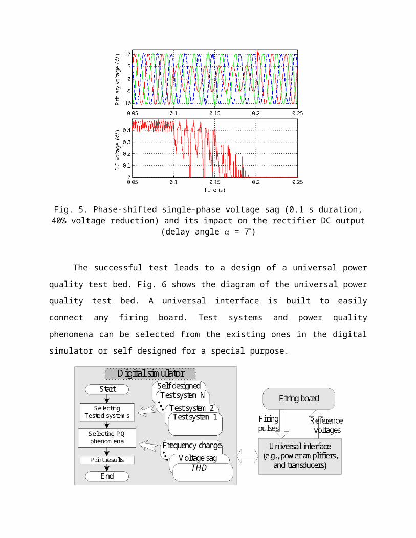
8 16 24-10

-8

-6

-4

-2

05th Harmonic

Time (hour)

Rea

l par

t (pu

) Bus30

x 10 -3

8 16 24-32

-30

-28

-26

-24

-225th Harmonic

Time (hour)

Imag

inar

y pa

rt (

pu)

Bus30

x 10 -3

8 16 24-18

-16

-14

-12

-10

7th Harmonic

Time (hour)

Rea

l par

t (pu

)

Bus30

x 10 -3

8 16 24-20

-18

-16

-14

-12

-107th Harmonic

Time (hour)

Imag

inar

y pa

rt (

pu)

Bus30

x 10 -3

8 16 24-12

-10

-8

-6

-4

-2 x 10-3 11th Harmonic

Time (hour)

Rea

l par

t (pu

) Bus30

8 16 240

2

4

6

8

1011th Harmonic

Time (hour)

Imag

inar

y pa

rt (

pu)

Bus30

x 10 -3

8 16 24-10

-8

-6

-4

-2

013th Harmonic

Time (hour)

Rea

l par

t (pu

)

Bus30

x 10 -3

8 16 240

2

4

6

8

1013th Harmonic

Time (hour)

Imag

inar

y pa

rt (

pu)

Bus30

x 10 -3

8 16 240

2

4

6

8

1017th Harmonic

Time (hour)

Rea

l par

t (pu

)

Bus30

x 10 -3

8 16 240

2

4

6

8

1017th Harmonic

Time (hour)

Imag

inar

y pa

rt (

pu)

Bus30

x 10 -3

Figure 4. Harmonic components of current injection at Bus 30

Table 3. errors between estimated and actual smoothed harmonic current profiles at bus 30

Harmonic

Order

Correlation

Coefficient

Maximum

Percentage

Error (%)

Mean Percentage Error (%)

BUS

30

5Real 0.6150 27.13 11.59

Imag 0.9640 6.39 2.21

7Real 0.9592 7.21 2.15

Imag 0.9525 7.55 2.66

11Real 0.9485 7.95 3.20

Imag 0.8817 19.39 8.47

13Real 0.9669 5.43 1.81

Imag 0.8787 15.07 6.02

17Real 0.8940 12.97 5.96

Imag 0.9398 10.18 3.14

Case 2In this case, the estimation process is based on fewer measurements in order to test the

effectiveness of the proposed algorithm for estimating the largest harmonic source in the

network. Using the same test system as in Fig. 1, two harmonic voltage measurements are

taken from bus 2 and 4 instead of seven measurements as in Case 1.

Estimation results for the harmonic source at bus 7 are given in Table 4. Using the ICA

algorithm, this harmonic load is estimated with a small error. Second output of the ICA

estimation can not be matched with other two harmonic sources at Bus 16 and 30, because the

correlation coefficients are small, i.e. 0.3516 and 0.4587.

Table 4. errors between estimated and actual smoothed harmonic current profiles at bus 7 with 2 harmonic measurements

Harmonic

Order

Correlation

Coefficient

Maximum

Percentage

Error (%)

Mean Percentage Error (%)

BUS

7

5Real 0.9982 3.29 1.00

Imag 0.9916 6.31 2.26

7Real 0.9949 6.20 2.02

Imag 0.9989 2.62 0.79

11Real 0.9989 2.09 0.90

Imag 0.9993 2.17 0.54

13Real 0.9977 5.21 1.06

Imag 0.9983 2.25 1.12

17Real 0.9417 16.68 6.48

Imag 0.9593 8.95 2.38

From the results given in Case 1 and 2, we can see that, the harmonic source with

harmonic current rating higher than the other system loads, can be estimated with a very good

range of error.

As future work, the impact of the location and number of measurements as well as the

number time steps per measurement on the accuracy of the estimation needs further

investigation.

5.8 - Conclusion

Independent Component Analysis is used to estimate the load profiles of harmonic

sources without prior knowledge of network topology and parameters. This method is based on

the statistical properties of loads. Statistical independence of loads is assured by separating the

fast and slow varying components in load profiles using a linear filter and by using only the fast-

varying component for the independent component analysis. The application of the proposed

algorithm to the modified IEEE 30-Bus test system shows that current profiles of harmonic

sources can be estimated using only a small number of harmonic voltage measurements.

The proposed method is quite promising for the application in a deregulated network

since the number of measurements is small and the measurements can be taken far from the

sources. Also this algorithm can be extended to find the minimum set of measurements to

reduce the measurements cost and increase estimation accuracy for the harmonic meter

placement problem.

Acknowledgment

The authors would like to acknowledge Huaiwei Liao’s help in the early stages of this work.

5.9 References

Chapter 6 - Prony Analysis for Power System Transient Harmonics

L. Qi, S. Woodruff, L. Qian and D. Cartes

6.1 - Introduction

Proliferation of nonlinear loads in power systems has increased harmonic pollution and

deteriorated power quality. Not required to have prior knowledge of existing harmonics, Prony

analysis detects frequencies, magnitudes, phases and especially damping factors of exponential

decaying or growing transient harmonics. Prony analysis is implemented to supervise power

system transient harmonics, or time varying harmonics. Further, to improve power quality

when transient harmonics appear, the dominant harmonics identified from Prony analysis are

used as the harmonic reference for harmonic selective active filters. Simulation results of two

test systems during transformer energizing and induction motor starting confirm the

effectiveness of the Prony analysis in supervising and canceling power system transient

harmonics.

In today’s power systems, the proliferation of nonlinear loads has increased harmonic

pollution. Harmonics cause many problems in connected power systems, such as reactive

power burden and low system efficiency. Harmonic supervision is highly valuable in relieving

these problems in power transmission systems. Further, harmonic selective active filters can be

connected in power distribution systems to improve power quality. Normally, Fourier

transform-based approaches are used for supervising power system harmonics. However, the

accuracy of Fourier transform is affected when these transient or time varying harmonics exist.

Without prior knowledge of frequency components, some of the harmonic filters require PLL

(Phase Locked Loops) or frequency estimators for identifying the specific harmonic frequency

before the corresponding reference is generated [1]-[4].

Prony analysis is applied as an analysis method for harmonic supervisors and as a

harmonic reference generation method for harmonic selective active filters. Prony analysis, as

an autoregressive spectrum analysis method, does not require frequency information prior to

filtering. Therefore, additional PLL or frequency estimators described earlier are necessary. Due

to the ability to identify the damping factors, transient harmonics can be correctly identified for

the Prony based harmonic supervision and harmonic cancellation. Two important operations in

power systems, energizing a transformer and starting of an induction motor [5]-[7], can be

studied for harmonic supervision and cancellation.

6.2 - Prony Theorem

Since Prony analysis was first introduced into power system applications in 1990, it has

been widely used for power system transient studies [8][9], but rarely used for power quality

studies. Prony analysis is a method of fitting a linear combination of exponential terms to a

signal as shown (1) [9]. Each term in (1) has four elements: the magnitude , the damping

factor , the frequency , and the phase angle . Each exponential component with a

different frequency is viewed as a unique mode of the original signal . The four elements of

each mode can be identified from the state space representation of an equally sampled data

record. The time interval between each sample is T.

(1)

Using Euler’s theorem and letting t = MT, the samples of are rewritten as (2).

(2)

(3)

(4)

Prony analysis consists of three steps. In the first step, the coefficients of a linear

predication model are calculated. The linear predication model (LPM) of order N, shown in (5),

is built to fit the equally sampled data record with length M. Normally, the length M

should be at least three times larger than the order N.

(5)

Estimation of the LPM coefficients is crucial for the derivation of the frequency,

damping, magnitude, and phase angle of a signal. To estimate these coefficients accurately,

many algorithms can be used. A matrix representation of the signal at various sample times can

be formed by sequentially writing the linear prediction of repetitively. By inverting the

matrix representation, the linear coefficients can be derived from (6). An algorithm, which

uses singular value decomposition for the matrix inversion to derive the LPM coefficients, is

called SVD algorithm.

(6)

In the second step, the roots of the characteristic polynomial shown as (7) associated

with the LPM from the first step are derived. The damping factor and frequency are

calculated from the root according to (4).

(7)

In the last step, the magnitudes and the phase angles of the signal are solved in the least

square sense. According to (2), equation (8) is built using the solved roots .

(8)

(9)

(10)

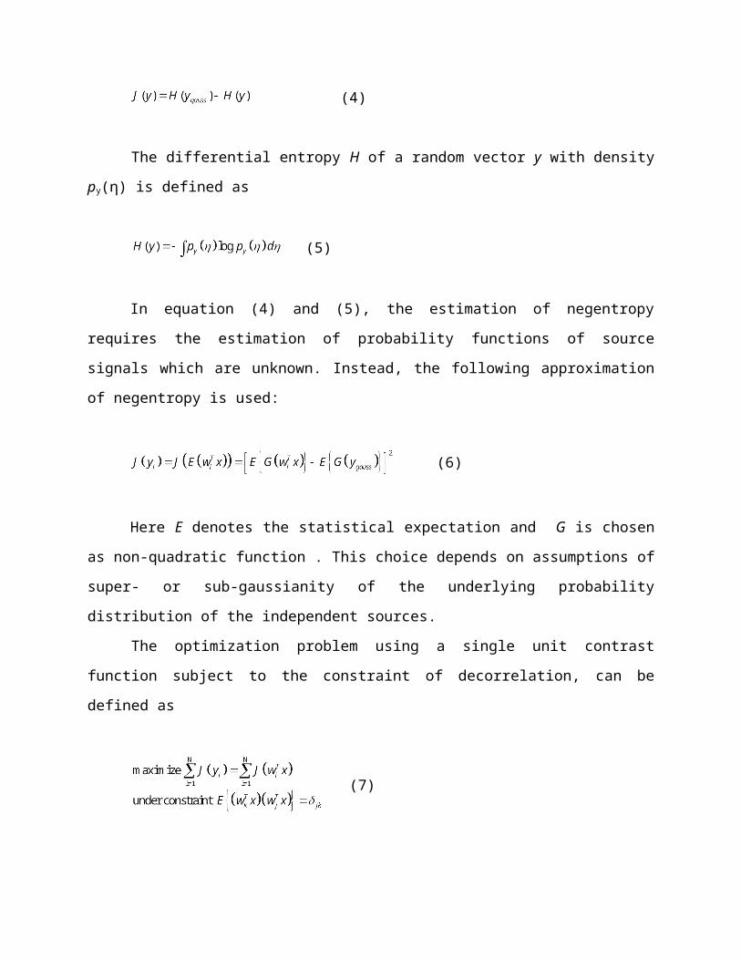
(11)

The magnitude and phase angle are thus calculated from the variables according to

(3).

The greatest advantage of Prony analysis is its ability to identify the damping factor of

each mode in the signal. Due to this advantage, transient harmonics can be identified

accurately.

6.3 Selection of Prony Analysis Algorithm

Three normally used algorithms to derive the LPM coefficients, the Burg algorithm, the

Marple algorithm, and the SVD (Singular value decomposition) algorithm [11]-[13], are

compared for implementing Prony analysis in transient harmonic studies. The non-recursive

SVD algorithm utilized the Matlab pseudo-inverse function pinv. This pinv function uses LAPACK

routines to compute the singular value decomposition for the matrix inversion [14]. To choose

the appropriate algorithm, the three algorithms are applied on the same signals with the same

Prony analysis parameters. The signals are synthesized in the form of (1) plus a relatively low

level of noise to approximate real transient signals. The sampling frequency is selected equal to

four times of the highest harmonic and the length of data is six times of one cycle of the lowest

harmonic [15]. Table 5 lists the estimation results from the three algorithms on one transient

signal. More estimation results on synthesized power system signals were derived by the

authors for different studies [16]. From comparison on the estimation results of various signals

to approximate power system transient harmonics, the SVD algorithm has the best overall

performance on all estimation results and thus is selected as the appropriate algorithm for

Prony analysis.

Table 5: Estimated Dominant Harmonics (EDH) on A Nonstationary Signal

EDH Ideal Burg Marple SVD

Frequencies (Hz) #1 60 60.1690 59.9986 59.9987

#2 300 298.2309 279.3917 299.9951

#3 420 419.3031 420.0081 420.0138

#4 660 657.8118 659.9380 659.9578

#5 780 779.1504 779.9914 780.0137

Damping factors (s-1)

#1 0 -0.0037 -0.0027 -0.0012

#2 -6 -1.3173 0.2127 -6.0403

#3 -4 -0.0940 0.1245 -4.0638

#4 0 -0.5625 -0.1881 -0.1097

#5 0 -3.4003 -0.6494 -0.1752

Magnitudes (A)

#1 1 1.0001 0.9997 1.0002

#2 0.2 0.1478 0.1441 0.2002

#3 0.1 0.0819 0.0809 0.1003

#4 0.02 0.0184 0.0203 0.0204

#5 0.01 0.0104 0.0107 0.0103

Phase Angles (Degree)

#1 0 3.1693 0.0320 3.1693

#2 45 79.0299 44.9906 45.0567

#3 30 41.4376 30.2150 29.9158

#4 0 36.8397 -0.8574 0.7913

#5 0 12.7567 0.1850 0.3631

6.4 Tuning of Prony Parameters

Since the estimation of data is an ill-conditioned problem [12][13], one algorithm could

perform completely differently on different signals. Therefore, Prony analysis parameters

should be adjusted by trial and error to achieve most accurate results at different situations.

Although the parameter tuning is a trial and error process, there are still some rules to follow. A

general guidance on parameter adjustment is given in the rest of this section.

A technique of shifting time windows by Hauer [5] is adopted for continuously detecting

dominant harmonics in a Prony analysis based harmonic supervisor. The shifting time window

for Prony analysis has to be filled with sampled data before correct estimation results are

derived. The selection of the equal sampling intervals between samples and the data length in

an analysis window depends on the simulation time step and the estimated frequency range.

The equal sampling frequency follows Nyquist sampling theorem and should be at least two

times of the highest frequency in a signal. Since the Prony analysis results are not accurate for

too high sampling frequency [15], two or three times of the highest frequency is considered to

produces accurate Prony analysis results. Similarly, the length of the Prony analysis window

should be at least one and half times of one cycle of the lowest frequency of a signal.

Besides the sampling frequency and the length of Prony analysis window, the LPM order

is another important Prony analysis parameter. A common principle is the LPM order should be

no more than one thirds of the data length [8][15]. The data length and LPM order could be

increased together in order to accommodate more modes in simulated signals. It is quite

difficult to make the first selection of the LPM order since the exact number of modes of a real

system is hard to determine. In our case studies, a guess of 14 is a good start. If the order is

found not high enough, the data length of the Prony analysis window should be increased in

order to increase the LPM order.

The general guidance for tuning Prony analysis parameters is applicable to other

applications of Prony analysis. Not requiring specific frequency of a signal for Prony analysis, the

tuning method is not sensitive to fine details of the signal and thus extensive retuning for

different types of transients in the same system is unlikely to be necessary for Prony analysis.

6.5 Prony Analysis and Fourier Transform

As described earlier, the Fourier transform is widely used for spectrum analysis in power

systems. However, signals must be stationary and periodic for the finite Fourier transform to be

valid. The following analysis explains why results from the Fourier transform are inaccurate for

exponential signals.

The general form of a nonstationary signal can be found in (1). If the phase angle of the

signal is equal to zero, and the magnitude is equal to unity, then the general form can be

simplified into the signal shown in (12). The initial time of the Fourier analysis is taken to be t0

and the duration of the Fourier analysis window is T, which is equal to the period of the analysis

signal for accurate spectrum analysis.

(12)

The Fourier transform during t0 to t0+T is calculated as (13). The first term on the right-

hand side of (13) is equal to zero according to (14). Therefore, the magnitude of the signal in

terms of the Fourier transform is given in (15). The ratio k between the magnitude of the

Fourier transform in (15) and the actual magnitude is shown as (16), which indicates the

average effect of the Fourier analysis window.

(13)

(14)

(15)

(16)

Let’s consider a fast damping signal and a slow damping signal with damping factors

equal to -100 and -0.01, respectively. If the frequency f is equal to 60Hz, then the duration T is

equal to 0.0167s. According to (16), the ratio k between the Fourier magnitude and the real

magnitude are derived as 0.4861 and 0.9999. Therefore, with rapid decaying factors, the

magnitude derived from Fourier transform is averaged by the analysis window and not even

close to its actual magnitude. If the damping factor is equal to zero, the ration k becomes one

and the Fourier magnitude exactly reflects the real signal magnitude. With rapidly decaying

signals, Fourier analysis results depend greatly on the length of the analysis window. For

example, if the time duration T of the analysis window is two cycles long and the damping ratio

is -100, then the ratio k decreases to 0.2888. Therefore, prior knowledge of the frequency

involved is quite important for selecting the proper length of the Fourier analysis window and

getting accurate results.

A conflict exists in selecting the length of the Fourier analysis window. In order to reduce

the error due to the average effect, the length of the Fourier analysis window should decrease.

However, the fewer periods there are in the record, the less random noise gets averaged out

and the less accurate the result will be. Some compromise must be made between reducing

noise effects and increasing Fourier analysis accuracy. The length of the Prony analysis window

is not as sensitive as the Fourier analysis window. If the frequency of an analyzed signal is

within a certain range, it is not necessary to change the length of the analysis window. A long

window can be used to deal with noise and still detect decaying modes accurately.

6.6 Case Studies

Using the SVD algorithm discussed in section C, two cases were studied to implement

Prony analysis for power quality study. The first case studies the harmonic supervision during

transformer energizing. The second case studies the harmonic cancellation during motor

starting. The test systems are realized in the simulation environment of PSIM and Matlab. The

parameters of the test systems can be found in the Appendix.

Case 1: Harmonic Supervision

Figure 1 shows the configuration of test system 1, which models a part of a transmission

system at the voltage level of 500 kV including a voltage source, a local LC load bank, and three-

phase transformer, and a harmonic supervisor. The voltages and currents at the transformer

primary side are inputs of the harmonic supervisor; while the outputs are the harmonic

description of the voltages and currents, which can be harmonic magnitudes and phase angles

from Fourier analysis or harmonic waveforms from Prony analysis.

Figure 1: Configuration of Test System 1

In our study, the Fourier transform analysis utilizes the function FFT provided in the

SimPowerSystems Toolbox in Matlab. One cycle of simulation has to be completed before the

outputs give the correct magnitude and angle since the FFT function uses a running average

window [17]. As described earlier, shifting time windows is used in Prony analysis for

continuously detecting dominant harmonics. In this Prony based harmonic supervisor for

transformer energizing, since the fundamental frequency is considered as the lowest frequency,

the time duration of Prony analysis window is 0.036 seconds, which is longer than two cycles of

the fundamental frequency. The time interval between any two windows is 0.6 ms. The

sampling frequency is 833 Hz, which is sufficient enough for identifying up to 13th harmonic in

the system. The data length within a time window is 60. The order of linear prediction model is

20, which is equal to one third of the data length.

The simulated system is designed to be resonant at forth harmonic [17]. Both even and

odd harmonic components are produced during the transformer energizing. Among them, the

second harmonic is dominant harmonic. The magnitudes of the harmonics during energizing

vary with time [5]. No abrupt changes are found in time varying harmonic magnitudes. An

exponential function thus is able to approximate these time varying harmonics.

Figure 2 shows the harmonic supervision results of test system 1 using the Prony

analysis and Fourier transform based harmonic supervisors. Figure 2(a) and Figure 2(b) show

the fundamental and 4th harmonic voltage waveform derived from Prony and the magnitudes

from FFT. Because there is no decaying or growing in the fundamental component, the

magnitude obtained from FFT agrees with the magnitude of the fundamental voltage waveform

from Prony. However, for the 4th harmonic, the magnitude from FFT is much smaller than that

from Prony since the 4th harmonic decays fast. Figure 2(c) and Figure 2(d) show the

fundamental and 2nd harmonic current from Prony analysis and the magnitudes from FFT. Due

to the slow decaying and growing speeds, the magnitudes from Prony analysis agree well with

the magnitudes from FFT.

0.04 0.06 0.08 0.1 0.12-500

0

500

Time (S)

Volta

ge (K

V)

PronyFFT

0.04 0.06 0.08 0.1 0.12-50

0

50

Time (S)

Volta

ge (K

V)

PronyFFT

(a) Fundamental Voltage (Phase A) (b) 4th Harmonic Voltage (Phase A)

0.05 0.1 0.15 0.2 0.25-1000

-500

0

500

1000

Time (S)

Cur

rent

(A)

PronyFFT

0.05 0.1 0.15 0.2 0.25-300

-200

-100

0

100

200

300

Time (S)

Cur

rent

(A)

PronyFFT

(c) Fundamental Current (Phase A) (d) 2nd Harmonic Current (Phase A)

Figure 2: Prony and FFT Results of Case 1

The effectiveness of the Prony based harmonic supervisor is verified from the results

shown earlier. From the comparison shown above, without damping or with small damping, the

harmonic supervision results from Prony analysis and FFT are almost equal in the sense of

harmonic magnitudes. With fast damping, Prony analysis derives more accurate harmonic

supervision results than FFT does.

Harmonic Cancellation

Figure 3 shows the configuration of test system 2, which models a part of a distribution

system at the voltage level of 480 V. The test system includes a voltage source, a nonlinear load

including an induction motor and a diode rectifier load, a harmonic selective active filter using a

three-phase active voltage source IGBT (Insulated Gate Bipolar Transistor) converter, and

controller systems associated with the active filter. The nonlinear load represents a type of load

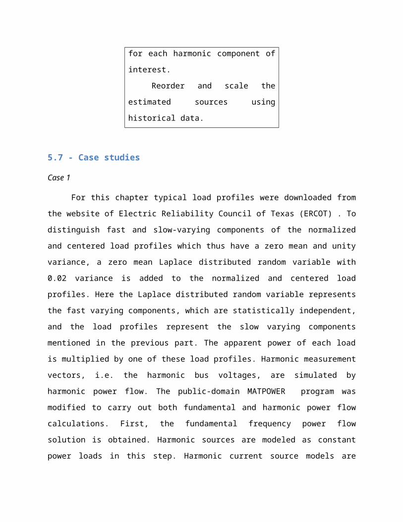
combination, induction motors plus power electronic loads, in power distribution systems. To

describe the detailed motor starting dynamics, the induction motor is modeled by a set of

nonlinear equations [17], which are different from the commonly used linear equivalent circuit

to model induction motors in power quality studies [5]. The motor has a constant load torque

of 0.2N.m.

Figure 3: Configuration of Test System 2

The control system of the active filter can be separated into two parts, one for

controlling harmonic reference generation using Prony analysis or Fourier transform and one

for controlling the DC link bus voltage. The dominant harmonics of the three phase load

currents are derived from Prony analysis or Fourier transform and used as the reference for the

harmonic selective active filter. To control DC bus voltage, a PI (Proportional Integral) controller

is used to generate the DC link current reference. Three hysteresis controllers then generate

gate signals for the IGBT converter.

As described earlier, some Prony analysis parameters used earlier in transformer

energizing are adjusted by trial and error to achieve most accurate results in motor starting. In

this Prony based active filter to cancel transient harmonics during motor starting, since there

could be sub-harmonics during motor starting, the time duration of the Prony analysis window

is 0.024 seconds. The sampling frequency is 2500 Hz, which is sufficient to identify up to the

20th harmonic in the system. With the careful selection of these Prony analysis parameters, the

spurious harmonics besides the dominant harmonics are small enough that their effects can be

neglected.

During motor starting, the magnitude of the starting current can become as high as

several times of the rated current. This high motor starting current contains mainly

exponentially decaying fundamental current and a small portion of decaying harmonic or sub-

harmonic currents. Due to the exponentially decaying fundamental current, the load voltage

changes exponentially. With this exponentially changing voltage supplied to the rectifier load,

the harmonic currents drawn by the rectifier load appear as exponentially changing harmonic

currents. Detecting and canceling harmonics in the total load currents during motor starting are

thus critical to overall power system reliability and power quality.

Table 6 shows the three most dominant frequencies identified from Prony analysis at

three selected time instants selected arbitrarily from the time duration before, during and after

motor starting transient. Because the 2nd harmonic current is induced by starting an induction

motor [5], it is found that the 2nd dominant harmonic current change from the 5th harmonic

current before motor starting to the 2nd harmonic current after motor starting. This 2nd

harmonic current is damped out during motor starting with a high damping factor. The

magnitudes of the 5th and 7th harmonic currents change exponentially during motor starting,

but are almost kept constant before and after motor starting transients. The magnitude of the

fundamental current increases after motor starting since the total load current increases with

the motor load added as a part of the system load.

Table 6: Estimated Dominant Harmonics (EDH) of Case 2

EDH T=0.1 T=0.1786 T=0.2403

Frequencies (Hz)

#1 60.0880 60.9739 60.0395#2 300.2141 121.2281 299.8692#3 420.4627 299.9159 420.9291

Magnitudes (A)#1 44.0179 82.5488 58.9011#2 8.8723 12.0627 9.2252#3 3.0207 8.8103 3.4445#1 0.0450 -14.6057 0.1782

Damping factors (s-1)

#2 0.2094 -116.4742 -0.1920

#3 0.4268 -2.8884 -0.5291

Figure 4 shows the simulation results of the transient harmonic cancellation

by the Prony based active filter during motor starting. At first, the system runs at steady state

with only ideal diode rectifier load connected. After the active filter takes action at 0.06 second,

the induction motor is switched into the test system at 0.12 second. The motor starting

transient lasts for several cycles and dies down approximately at 0.2 second. The test system

finally settles down at steady state with both motor and diode rectifier load connected. The

stationary harmonic cancellation before and after motor starting has been verified by the

authors [15]. The harmonic cancellation by the Prony filter and the Fourier filter during motor

starting is compared in Figure 4(c) and Figure 4(d). It is seen that the improvement of the

source current by the Fourier based active filter is much less than the improvement by the

Prony based filter.

0.05 0.1 0.12 0.144 0.2 0.25-600

-400

-200

0

200

400

600

Time (S)

Cur

rent

(A)

Phase APhase BPhase C

motor starting

0.06 0.08 0.1 0.12 0.144 0.18 0.2 0.22 0.24

-300

-200

-100

0

100

200

Time (S)

Cur

rent

(A)

Actual Estimated

(a) Source Currents (b) Load Currents (Phase A)

0.12 0.13 0.14 0.15 0.16 0.17 0.18 0.19

-100

-50

0

50

100

150

200

250

300

Time (S)

Cur

rent

(A)

with active filterwithout active filter

0.12 0.14 0.16 0.18 0.2

-150

-100

-50

0

50

100

150

200

250

300

Time (Current)

Cur

rent

(A)

with active filterwithout active filter

(c) Source Currents (Phase A) (d) Source Currents Filter (Phase A)

During Motor Starting (Prony) During Motor Starting (FFT)

Figure 4: Simulation Results of Case 2

The effectiveness of the Prony-based harmonic selective active filter to cancel transient

harmonics during motor starting is verified. Using the active filter, the dominant 2nd, 5th and 7th

harmonics in the load currents are cancelled and the power quality during motor starting is

improved. Due to the length of Prony analysis window, it is observed in Figure 4(b) that there

are oscillations in the estimated load current at the beginning of motor starting.

6.7 Conclusions and Future Work

The effectiveness of the Prony analysis is verified for the harmonic supervision and

cancellation when transient or time varying harmonics exhibit in power systems. The unique

features of Prony analysis, such as frequency identification without prior knowledge of

frequency and the ability to identify damping factors, are useful to power system quality study.

Further studies can be carried out for power quality study. Just as Prony analysis was used with

harmonic selective active filters, Prony analysis may be applied to other measures to improve

power quality. In this study, the computational speed of the non-recursive SVD algorithm for

Prony is slow. With more efficient algorithms developed, Prony analysis can be applied for

online harmonic monitoring and harmonics cancellation using Real-Time Hardware-in-Loop (RT-

HIL) technology. Due to the insufficient information input into Prony analysis, inaccurate

harmonic estimation from Prony analysis may adversely affect controllers at the beginning of

transient periods. These disadvantages of applying Prony analysis are being considered and will

be improved in future studies.

Appendix

Table A.1: Parameters of Source of Test System 1

VRMSLL (KV) f (Hz) RS ( ) LS (H)

500 60 5.55 0.221

Table A.2: Parameters of A Local Capacitive Load of Test System 1

R ( ) C (F)

0.6606 0.0011

Table A.3: Parameters of A Three-Phase Transformer of Test System 1

R1 ( ) L1 (H) R2 ( ) L2 (H) RM ( ) Ratio (KV/KV)

1.1111 44.4444 0.2351 9.4044 0.041 500/230

Table A.4: Transformer Saturation Characteristic of Test System 1

(p.u.) I (p.u.)

0 0

1.20 0.0024

1.52 1.0

Table A.5: Parameters of Source of Test System 2

VRMSLL (V) f (Hz) RS ( ) LS (H)

480 60 10-5 10-6

Table A.6: Parameters of A Six-Pole Induction Motor of Test System 2

Rs ( ) Ls (H) Rr ( ) Lr (H) LM (H) J (kgm2)

0.294 0.00139 0.156 0.00074 0.041 0.4

Table A.7: Parameters of A Rectifier Load of Test System 2

RL ( ) CL (F) RLD ( ) LLD (H)

15 0.004 0.001 0.003

Table A.8: Parameters of An Active Filter of Test System 2

VRef (V) Cdc (F) RAF ( ) LAF (H)

800 0.002 0.0001 0.002

Table A.9: Parameters of A PI Controller of Test System 2

KP KI

1.0 1.0

Table A.10: Parameters of A Hysteresis Controller of Test System 2

Ton (S) Toff (S) Gon Goff

0.001 -0.001 1 0

6.8 References

[1] Po-Tai Cheng, Bhattacharya S., and Divan D., “Operations of the dominant harmonic active filter (DHAF) under realistic utility conditions,” IEEE Transactions on Industry Applications, Volume: 37, Issue: 4, July-Aug. 2001, Pages: 1037 – 1044

[2] Po-Tai Cheng, Subhashish Bhattacharya and Deepak M. Divan, “Control of Square-Wave Inverters in High-Power Hybrid Active Filter Systems,” IEEE Transactions on Industry Applications, Vol.34, NO.3, May/June 1998.

[3] Po-Tai Cheng, Subhashish Bhattacharya and Deepak D. Divan, “Line Harmonics Reduction in High-Power Systems Using Square-Wave Inverters-Based Dominant Harmonic Active Filter,” IEEE Transactions on Power Electronics, Vol. 14, NO.2, March 1999.

[4] Po-Tai Chen, Subhashish Bhattacharya and Deepak Divan, “Experimental Verification of Dominant Harmonic Active Filter for High-Power Applications,” IEEE Transactions on Industry Applications, Vol.36, NO.2, March/April 2000.

[5] J. Arrillaga, B. C. Smith, N. R. Watson, A. R. Wood, Power System Harmonic Analysis, John Wiley & Sons, 1997.

[6] V. S. Moo, Y. N. Chang, P. P. Mok, “A Digital Measurement Scheme for Time-Varying Transient Harmonics”, IEEE Trans. Power Delivery, Vol. 10, Issue 2, April, 1995, pp. 588-594.

[7] S. J. Huang, C. L. Huang, C. T. Hsieh, “Application of Gabor Transform Technique to Supervise Power System Transient Harmonics”, IEE Proceedings Generation, Transmission and Distribution, Vol. 143, Issue 5, Sept 1996, pp. 461-466.

[8] J. F. Hauer, C. J. Demeure, and L. L. Scharf, "Initial Results in Prony Analysis of Power System Response Signals," IEEE Trans. Power Systems, Vol. 5, No. 1, pp. 80-89, Feb. 1990.

[9] O. Chaari, P. Bastard, and M. Meunier, “Prony's method: An Efficient Tool for the Analysis of Earth Fault Currents in Petersen-coil-protected Networks”, IEEE Trans. On Power Delivery, July 1995, Vol. 10, I. 3, pp. 1234-1242.

[10] F. B. Hildebrand, Introduction to Numerical Analysis, McGraw-Hill Book Company, Inc., 1956.

[11] L. Marple, “A New Autoregressive Spectrum Analysis Algorithm,” IEEE Trans. Acoustics, Speech, and Signal Processing, Vol. ASSP-28, No. 4, August 1980.

[12] P. Barone, “Some Practical Remarks on the Extended Prony’s Method of Spectrum Analysis,” Proceedings of IEEE, Vol. 76, No. 3, March 1988, pp. 284-285.

[13] S. M. Kay, S. L. Marple, “Spectrum Analysis – A Modern Perspective,” Proc., IEEE, Vol. 69, No. 11Nov. 1981, pp. 1380-1419.

[14] E. Anderson, Z. Bai, C. Bischof, et al., LAPACK User's Guide [http://www.netlib.org/lapack/lug/lapack_lug.html], Third Edition, SIAM, Philadelphia, 1999.

[15] M. A. Johnson, I. P. Zarafonitis, and M. Calligaris, “Prony Analysis and Power System Stability Some Recent Theoretical and Application Research”, Proceeding of 2000 IEEE PES General Meeting, Vol. 3, July 2000, pp. 1918-1923.

[16] L. Qi, L. Qian, D. Cartes, and S. Woodruff, “Initial Results in Prony Analysis for Harmonic Selective Active Filters”, Proceeding Of 2006 IEEE PES General Meeting, June 2006, Montreal, QC, Canada.

[17] Hydro-Quebec, TransEnergie, SymPowerSystems For Use With Simulink, Online only, The Mathworks Inc, July 2002.

[18] Powersim Inc., PSIM User’s Guide Version 6.0, Powersim Inc., June 2003.

Chapter 7 - Empirical Mode Decomposition - Enhancements to the

Hilbert-Huang Method for Power System Applications

N. Senroy, S. Suryanarayanan and P. F. Ribeiro

7.1 Introduction

With the pervading application of power electronics and other non-linear time-varying

loads and equipment in modern power systems, distortions in line voltage and current are

becoming an increasingly complex issue. In tightly coupled power systems such as the

integrated power system (IPS) onboard all-electric ships and islanded micro-grids, the

estimation and visualization of time-varying waveform distortions present an interesting

research avenue [1]. Accurately estimating time-varying distorted voltage and current signals

will help in determining innovative power quality indices and thresholds, equipment derating

levels and adequate mitigation methods including harmonic filter design. In this context, it is no

longer appropriate to use “harmonics” to describe the higher modes of oscillations present in

non-stationary and nonlinear waveform distortions. Harmonics imply stationarity and linearity

among the modes of oscillations while the focus of this chapter, is on time-varying waveform

distortions. Key issues specific to the problem of estimating time-varying modes in distorted

line voltages and currents are: (a) distortion magnitudes are small, and typically range from 1-

10% (voltage) and 10-30% (current) of the fundamental, (b) the fundamental frequency may

not be constant during the observation, due to load fluctuations and system transients, (c)

typical distortion frequencies of interest in electric power quality studies may lie within an

octave – posing a challenge of separation.

Estimating the modes existing in a complex distorted signal may be reposed as an

instantaneous amplitude and frequency tracking problem. What is the degree to which the

time-frequency-magnitude resolution of the participant modes, in a distorted voltage/current

signal, may be realized? Research has already indicated the role of the uncertainty principle in

limiting the performance of time-frequency distributions [2]. This chapter approaches the

problem as follows:

1. Adaptively decompose the distorted signal into mono-component forms existing at

different time-scales,

2. Estimate instantaneous frequencies and amplitudes of each of the separated

components,

3. Localize the temporal variations in these amplitudes and frequencies accurately on

the time scale.

The Hilbert-Huang (HH) method, including the empirical mode decomposition (EMD),

has been developed as an innovative time-frequency-magnitude resolution tool for non-

stationary signals [3]. EMD is an adaptive and data driven multi-resolution technique, in which a

multi-component waveform is resolved into several components. These components, referred

to as intrinsic mode functions (IMF), are expected to be mono-component in nature.

Application of Hilbert transform yields their analytic forms, from which their instantaneous

amplitudes and frequencies can be extracted. However, the original EMD technique fails to

separate participating modes whose instantaneous frequencies simultaneously lie within an

octave.

The use of a masking signal based EMD was initially proposed to improve the filtering

characteristics of the EMD [4]. In this chapter, a hybrid algorithm is presented for building

appropriate masking signals for applying EMD to distorted signals [5]. The improved algorithm

employs fast Fourier transform (FFT) to develop masking signals to apply in conjunction with

the EMD. Once a masking signal is constructed, the EMD application follows the method of [4].

Since the masking signal based EMD may not always guarantee mono-component IMFs, further

demodulation is recommended, after applying the Hilbert transform. Another alternative to the

masking signal based EMD is frequency shifting, suggested in conjunction with EMD to enhance

its discriminating capability [6]. The proposed enhancements focus on signals, typically found in

power quality applications, with the following characteristics:

1. Time-varying modes whose instantaneous frequencies may lie in the same octave

simultaneously,

2. Weak higher frequency signals not ‘recognizable’ by conventional EMD.

The rest of the chapter is divided into sections as follows. Section II discusses different

approaches to the problem of estimating time-varying waveform distortions. Section III

introduces the original Hilbert-Huang method, along with its limitations. The masking signal

based EMD is presented in detail in this section, along with the demodulation techniques

suggested for narrowband IMFs. Section IV employs a synthetic signal representative of signals

in power systems, to demonstrate the masking signal based EMD. The frequency shifting

technique used in conjunction with EMD is presented in Section V. Section VI is the concluding

section.

7.2 Estimating Non-stationary Distortions

The fast Fourier transform (FFT) technique is adopted as a signal processing tool, when

linearity and stationarity are satisfied by the participating modes in a distorted waveform [7].

FFT serves as a computationally efficient and accurate technique to decompose such a distorted

waveform into sinusoidal components. In the event of nonlinear modal interaction, the FFT

spectrum may be spread over a wider range that may lack physical significance. When the

distortions are non-stationary, FFT may be computed over a sliding window [8]. The fixed

window width restricts the time-frequency resolution of this method. The sliding window based

ESPRIT method, i.e. estimation of signal parameters via rotational invariance techniques, can

separate closely spaced harmonics/inter-harmonics [9]. However, for non-stationary

distortions, post-processing techniques are required to ensure continuity in the time-frequency

estimation in consecutive windows.

The wavelet transform is a mathematical tool proposed to identify modes of non-

periodic oscillations, as well as those that evolve in time [10]. Kernel functions referred to as

wavelets are employed to obtain a multiresolution decomposition of the signal into oscillations

at different time scales. Thus, different time resolutions are used to adapt to different

frequencies. The choice of the mother wavelet depends on the signal being analyzed. The

wavelet transform is capable of separating individual frequency components, provided they are

sufficiently apart on the frequency scale. The wavelet technique has been employed to power

quality issues with success [11], [12]. An extension of the wavelet transform, the S-transform, is

based on a moving, scalable, localizing Gaussian window [13]. The S-transform has superior

phase-frequency-time localizing properties and has been applied to analyzing power quality

disturbances [14], [15]. In this chapter, the S-transform is used as a benchmark against which

the improved HH method is compared. The parameters of the S-transform used in this chapter

are as follows: the dilation factor of the wavelet is defined as the straightforward inverse of

frequency, and the transform is performed on the analytic form of the real valued data [13].

The Hilbert-Huang (HH) method was first proposed for geophysics applications [16]. It

has, since then, been applied to problems in biomedical engineering [17], image processing

[18], and structural safety [19]. In power systems, the HH method has been applied to identify

instantaneous attributes of torsional shaft signals [20] and to analyze interarea oscillations [21],

[22]. The empirical mode decomposition method has also been used to detect and localize

transient features of power system events [23]. Research is ongoing to provide an analytical

basis of the EMD [24].

7.3 Modified Hilbert Huang Technique

The original HH method has two parts. In the first part, a distorted waveform is

decomposed using EMD into multiple intrinsic mode functions (IMFs) that possess well-

behaved Hilbert transforms. Each IMF is defined by two principal characteristics – (a) its mean is

zero; (b) the number of local extrema must be equal to, or differ by at most 1 from the number

of zero crossings within an arbitrary time window. In the second part of the original HH

method, Hilbert transform is applied to obtain the instantaneous frequencies and amplitudes

existing in the individual IMFs. The details of the Hilbert-Huang method along with some

variations and other improvements are in [3], [19], [25]. This section briefly describes the

original EMD method and its performance while separating frequencies lying within one octave

(typical in power quality signals). To improve its performance, the need for masking signals has

been suggested in [4]. An innovative FFT based algorithm has been proposed to construct

appropriate masking signals to apply with the EMD [5]. A post processing demodulation

technique has also been proposed [5].

Empirical mode decomposition to obtain IMFs

The underlying principle of the Huang’s EMD method is the concept of instantaneous

frequency defined as the derivative of the phase of an analytic signal [26]. A mono-component

signal, by definition, has a unique well-defined and positive instantaneous frequency

represented by the derivative of the phase of the signal. A signal, with multiple modes of

oscillation existing simultaneously, will not have a meaningful instantaneous frequency.

Accordingly, a distorted signal must be decomposed into its constituent mono-component

signals before the application of Hilbert transform to calculate the instantaneous frequency.

The essence of EMD is to recognize oscillatory modes existing in time scales defined by

the interval between local extrema. A local extremum point is any point on the signal where its

derivative is zero, and its second derivative non-zero. The term local is used to differentiate it

from a global extremum point. For instance, within an observation window, there may be

several local extrema, however only one global maximum and global minimum point may be

present. Once the time scales are identified, IMFs with zero mean are sifted out of the signal.

The steps comprising the EMD method are as follows:

A1. Identify local maxima and minima of distorted signal, s(t),

A2. Perform cubic spline interpolation between the maxima and the minima to obtain the

envelopes eM(t) and em(t), respectively,

A3. Compute mean of the envelopes,

2tete

tm mM

,

A4. Extract c1(t) = s(t) - m(t),

A5. c1(t) is an IMF if the number of local extrema of c1(t), is equal to or differs from the

number of zero crossings by one, AND the average of c1(t) reasonably zero. If c1(t) is

not an IMF, then repeat steps A1-A4 on c1(t) instead of s(t), until the new c1(t)

obtained satisfies the conditions of an IMF,

A6. Compute the residue, r1(t) = s(t) – c1(t),

A7. If the residue, r1(t), is above a threshold value of error tolerance, then repeat steps A1-

A6 on r1(t), to obtain the next IMF and a new residue.

In practice, an appropriate stopping criterion, in step A5, avoids ‘over-improving’ c1(t) as

that can lead to significant loss of information [25]. The first IMF obtained, consists of the

highest frequency components present in the original signal. The subsequent IMFs obtained,

contain progressively lower frequency components of the signal. If n orthogonal IMFs are

obtained in this iterative manner, the original signal may be reconstructed as,

(1)

The final residue exhibits any general trends followed by the original signal.

Separation of modes of oscillation

In experiments conducted on fractional Gaussian noise the EMD technique has been

found to behave like a data driven dyadic filter bank [27]. Further experiments established the

ability of the EMD method to decompose white noise into IMFs whose frequency spectrum

comprises an octave [28]. The mean frequencies of the extracted IMFs show a doubling

phenomenon. It is worthwhile here to note the similarity between an IMF and a real-zero (RZ)

signal as defined by [29]. Bandpass signals whose zeros are distinct and real are called RZ

signals. Further, Logan, in [30], examined a subclass of bandpass signals that have no common

zeros between the signal and its Hilbert transform, other than real simple zeros. If the

bandwidth of such a signal is less than an octave, the signal is completely described by its zero

crossings (upto a multiplicative constant). An IMF would fall in this subclass of signals. The

implication is that if there are two modes coexisting in a signal, whose frequencies lie within an

octave of each other, the straightforward application of the EMD method is unable to separate

the two modes.

Consider a synthetic signal [6], of length 0.2 s and sampled at 20 kHz. The signal consists

of a 60 Hz fundamental component of magnitude 1.0 p.u. The signal is distorted by 120 Hz, 300

Hz and 420 Hz frequency components. A range of distorted signals was built by varying the

magnitude of distortions from 0.01 p.u to 0.1 p.u. All the distorted signals were kept stationary.

Masking signals of frequencies 720 Hz and 420 Hz were used along with EMD to extract only the

first IMF. In the presence of distortions due to a 420 Hz and a 300 Hz component, it was desired

to include only the 420 Hz component in the first IMF using the 720 Hz masking signal.

However, traces of the 300 Hz component are bound to be extracted as shown in the

demonstrations. Similarly, in the presence of a 300 Hz and a 120 Hz distortion, the 420 Hz

masking signal would include most of the 300 Hz component in the second IMF along with

some of the 120 Hz component, during EMD. The amplitude of the masking signal determines

its effectiveness in excluding/including lower frequency components in the first IMF during

EMD. Large amplitudes of the masking signal would include undesirable lower frequency

components in the IMF, while small amplitudes of the masking signal may not adequately

include the target frequency component in the IMF.

Separating 420 Hz from 300 Hz

Analyses done on a 60 Hz fundamental distorted by a 300 Hz and 420 Hz component are

presented first. The masking signal frequency is chosen to be 720 Hz because it shares an

octave with 420 Hz but not the 300 Hz component. The percentages of 300 Hz and 420 Hz

components, extracted in the first IMF using EMD with the masking signal of 720 Hz, are shown

in Fig. 1. The amplitude of the masking signal is plotted on the x-axes, while the original

magnitudes of the components in the distorted signal are plotted on the y-axes. The objective is

to minimize the extraction of the 300 Hz component, and maximize the extraction of the 420 Hz

component in the first IMF.

absolute amplitude of 720 Hz masking signal

orig

inal

mag

nitu

de

of 3

00 H

z co

mpo

nent

0.1 0.2 0.3 0.4 0.5 0.6 0.7 0.8 0.9 1

0.02

0.04

0.06

0.08

0.1

absolute amplitude of 720 Hz masking signal

orig

inal

mag

nitu

de

of 4

20 H

z co

mpo

nent

0.1 0.2 0.3 0.4 0.5 0.6 0.7 0.8 0.9 1

0.02

0.04

0.06

0.08

0.1

10

20

30

40

50

60

70

80

90

100

B

C

A

DE

F

Fig. 1. Percentage of 300 Hz and 420 Hz component extracted in the first IMF using a 720 Hz masking signal [6]. The absolute amplitude of masking signal is plotted on the x-axis, original content of the 300 Hz and 420 Hz components in the signal are plotted on the y-axis of the top and bottom plots respectively.

As evident from Fig. 1, an extremely weak masking signal (<0.05 p.u) is undesirable as it

would not affect the EMD process, and both 300 Hz and 420 Hz components are extracted

entirely in the first IMF (regions A and E in the top and bottom plots). In the presence of a

relatively stronger masking signal (>0.05 p.u), some of the 300 Hz component (upto 21%) is

included in the first IMF (region B). However, if the masking signal is not strong enough, the 420

Hz component is not sufficiently included in the first IMF, which is undesirable (region D). If the

masking signal is sufficiently strong, the entire 420 Hz signal is included in the first IMF (region

C), which is part of the desired objective of using the masking signal. However, an unavoidable

300 Hz component is bound to be included along with the 420 Hz component (region B), which

may be minimized. In the presence of a too strong masking signal, the 300 Hz will also be

included in the first IMF entirely (region F), which is undesirable. In summary, the masking

signal magnitude must be selected according to the regions B and C in the top and bottom plots

of Fig. 1.

Separating 300 Hz from 120 Hz

Fig. 2 shows the scenario when a 60 Hz signal (magnitude 1.0 p.u.) is distorted by a 300

Hz and 120 Hz component. Even though 120 Hz and 300 Hz do not lie in the same octave, a

masking signal is nevertheless required to accentuate their distortions to be recognized by the

EMD process. A 420 Hz masking frequency was used because it lies in the same octave with 300

Hz and sufficiently far from 120 Hz. The original absolute magnitudes of the two components

were varied from 0.01 p.u. to 0.1 p.u. while the masking signal magnitude was varied from 0.01

p.u. to 1.0 p.u. The objective here is to minimize the extraction of the 120 Hz component, and

maximize the extraction of the 300 Hz component in the first IMF.

absolute amplitude of 420 Hz masking signal

orig

inal

mag

nitu

de o

f 120

Hz

com

pone

nt

0.1 0.2 0.3 0.4 0.5 0.6 0.7 0.8 0.9 1

0.02

0.04

0.06

0.08

0.1

absolute amplitude of 420 Hz masking signal

orig

inal

mag

nitu

de o

f 300

Hz

com

pone

nt

0.1 0.2 0.3 0.4 0.5 0.6 0.7 0.8 0.9 1

0.02

0.04

0.06

0.08

0.1

10

20

30

40

50

60

70

80

90

100

A

B

C

D

EF

Fig. 2. Percentage of 120 Hz and 300 Hz component extracted in the first IMF using a 420 Hz masking signal [6]. The absolute amplitude of masking signal is plotted on the x-axis, original content of the 120 Hz and 300 Hz components in the signal are plotted on the y-axis of the top and bottom plots respectively.

In Fig. 2, regions A and F on the top plot and bottom plot respectively, indicate

situations where an extremely weak masking signal (less than 0.05 p.u.) has no effect on the

EMD process. Hence, both 120 Hz and 300 Hz components get extracted in the first IMF, in the

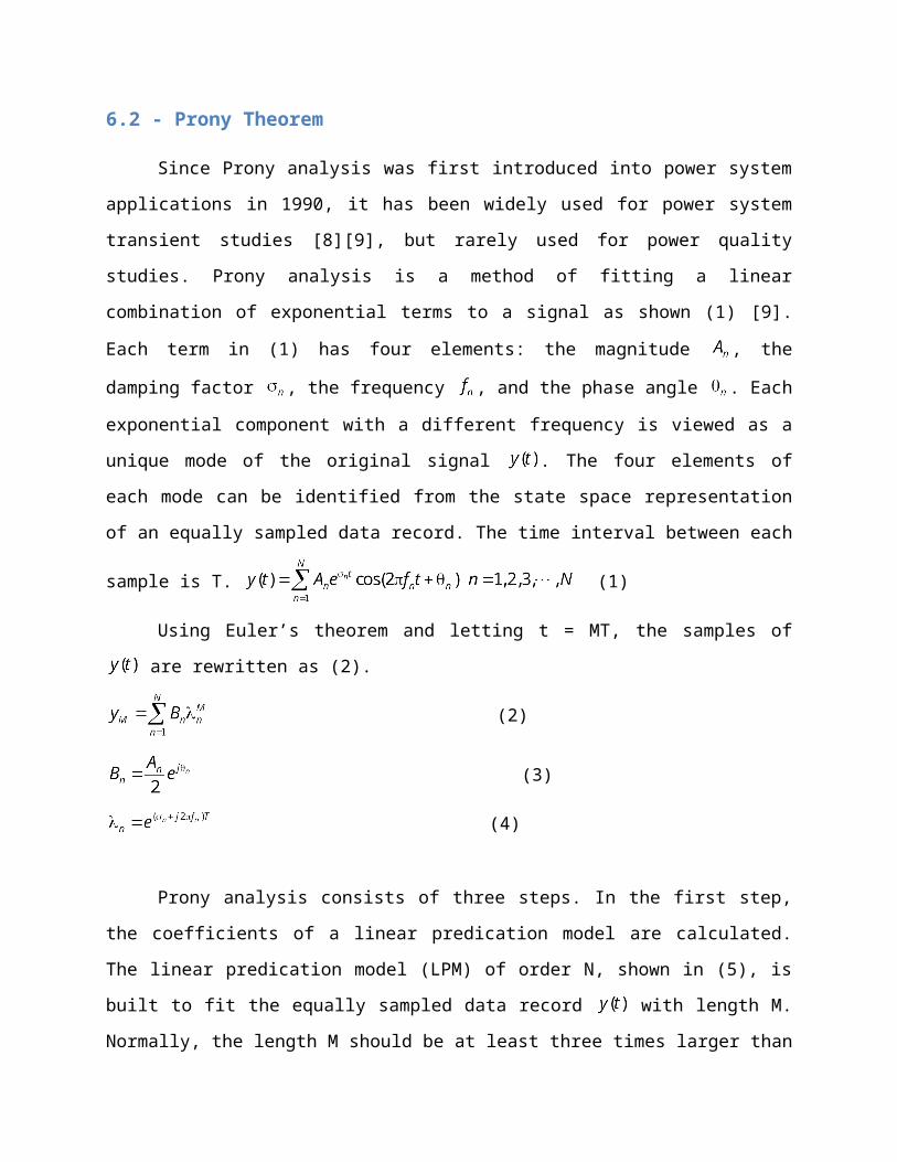
presence of such an extremely weak masking signal. When the masking signal is relatively

stronger but not strong enough (<0.1 p.u.), it extracts 300 Hz frequency component

insufficiently (region E in lower plot). However, when the masking signal magnitude is

sufficiently strong as in region D in the bottom plot, it extracts the entire 300 Hz component,

which is the desired objective of using a masking signal. The corresponding region on the top

plot is B, which shows an inevitable extraction of 2% of the 120 Hz in the first IMF. If the

masking signal is too strong, it extracts the entire 120 Hz component in addition to the 300 Hz

component in the first IMF (region C in the upper plot), which is undesirable.

7.5 Algorithm for appropriate masking signal to separate higher frequencies

A typical distorted power quality waveform consists of weak higher frequency modes

whose frequencies may share the same octave. The FFT spectrum of the signal yields its

approximate modal content. Masking signals are then required to separate modes of

oscillations whose frequencies lie within the same octave, and to accentuate weak higher

frequency signals so that they may be sifted out during the EMD. The appropriate masking

signals are constructed as follows [5].

C1. Perform FFT on the distorted signal, s(t), to estimate frequency components f1, f2,…, fn,

where f1< f2< …< fn,. Note: f1, f2,…, fn, are the stationary equivalents of the possibly time-

varying frequency components,

C2. Construct masking signals, mask2, mask3… maskn, where maskk (t) = Mk × sin(2 π (fk + fk -1) t).

An effective value of Mk is 5.5 × magnitude of fk obtained in FFT spectrum. The value of Mk is

empirical,

C3. Obtain two signals s(t)+maskn and s(t)–maskn. Perform EMD (steps A1–A5 from Section III-A)

on both signals to obtain their first IMFs only, IMF+ and IMF–. Then c1(t) = (IMF+ + IMF–)/2,

C4. Obtain the residue, r1(t) = s(t) – c1(t),

C5. Perform steps C3–C4 iteratively using the other masking signals and replacing s(t) with the

residue obtained, until n-1 IMFs containing frequency components f2 , f3 ,… fn are extracted.

The final residue rn(t) will contain the remaining component f1.

From the examples presented above, it is clear that even with masking signals EMD may

not produce sufficiently narrow band IMFs. The instantaneous frequency of such an IMF does

not hold much physical meaning when related to power system events and phenomena. In such

scenarios, some post-processing demodulation is required to extract meaningful instantaneous

frequencies and amplitudes.

7.6 Amplitude demodulation of IMF

Each IMF extracted using the masking signal based EMD contains a dominant high

frequency component, along with a remnant lower frequency component. The amplitude and

instantaneous frequency, extracted by Hilbert transform, shows a resultant modulation. This

section presents a technique to separate such an IMF into its components. Consider the

amplitude modulated (AM) signal,

(2)

where, ω2 > ω1. The Hilbert transform of s(t) is sH(t), and the analytical signal, corresponding to

s(t), is

(2)

where A(t) is the instantaneous magnitude and φ(t) is the instantaneous phase. From (2), the

instantaneous magnitude is

(3)

In a modulated signal, the local extrema points may be obtained as,

(4)

Apply cubic spline fitting among the local extrema points to obtain two envelopes

corresponding to the maximum envelope, Γmax, and the minimum envelope, Γmin, of the

amplitude. The true amplitudes of the two components are then

(5)

From (2), the instantaneous frequency of the signal is defined as . Also,

(6)

For the specific case of a modulation between two pure tones, the instantaneous frequency is,

21 2 1 2 2

1 2 21 2 1 2 1 2

( ) ( ).cos ( )( )

( ) ( ) 2 ( ) ( ).cos

A t A t t A tt

A t A t A t A t t

(7)

Substituting in (7),

(8)

From (3), the locally maximum magnitude occurs at , when . At this

instant, the instantaneous frequency from (8) is

(9)

Similarly, the locally minimum magnitude occurs at , when . The

instantaneous frequency at this instant in time is

(10)

Given the instantaneous magnitude and frequency for each IMF, the modulating

frequencies may be calculated by solving equations (9) or (10). The amplitudes of the

modulating components can be calculated from (5).

A flowchart, shown in Fig 3, describes the complete improved HH algorithm for

extracting all the frequency components in a distorted signal [5].

FFT to constructmasking signals

Masking signals{mask2, …, maskn}

EMD EMDr1(t) EMD rn(t)

c1(t) from r1(t)

Hilbertspectralanalysis

Distorted waveformfrom measurements

Demodulation Instantaneousamplitude & frequency

s(t)r2(t)

Distorted signal residue

Fig 3. Flowchart to compute high frequency distortion components in a distorted signal, using improved HH method [5].

7.7 Demonstration

The ability of the masking signal based EMD to separate the components present in a

non-stationary distorted signal is demonstrated in this section. Synthetic data is used to

validate the improved HH method [5]. A time series was constructed (sampled at 20 kHz) with a

fundamental frequency of 60 Hz and magnitude 1.0. Time varying 300 Hz, 420 Hz and constant

inter-harmonic 610 Hz components, with magnitudes shown in Table I, were used to distort the

60 Hz signal. The signal along with its FFT spectrum, containing only the higher frequency

modes, is plotted in Fig. 4. As seen in Fig. 4, the time-varying nature of the synthetic waveform

introduces spurious energy spread around the dominant frequencies in the FFT. The objective is

to extract the magnitudes and frequencies of all modes higher than the fundamental mode.

Table I

DETAILS OF SYNTHETIC DATA

Time (s) Magnitude of 300 Hz Magnitude of 420 Hz Magnitude of 610 Hz

0.0 - 0.1 0.05 0.03

0.020.10005-0.15 0.07 0.06

0.15005-0.25 0.09 0.05

0.25005-0.3 0.06 0.07

0.30005-0.4 0.05 0.04

The S-transform was used to analyze the data. A contour plot obtained from the S-

transform shows a significant frequency spread. A 120 Hz moving average filter was employed

to smooth the results. The spread of frequencies precludes a reliable estimate of the actual

modes present in the data. The amplitudes of a range of frequencies from 247.5-672.5 Hz are

plotted in Fig 5. While the amplitude tracking of the 300 Hz, 420 Hz and 610 Hz is good

(artificially highlighted curves), the estimation process clearly introduces fictitious components

(artificially greyed).

0 0.05 0.1 0.15 0.2 0.25 0.3 0.4

-1

0

1

time (s)

distorted synthetic signal

120 180 240 300 360 420 480 540 600 6600

0.02

0.04

0.06

0.08

frequency (Hz)

FFT of distorted synthetic signal

Fig 4. Synthetic data of Table I along with its FFT spectrum from 180 Hz to 840 Hz [5]. The vertical axes are in absolute magnitude.

0 0.05 0.1 0.15 0.2 0.25 0.3 0.35 0.40.01

0.02

0.03

0.04

0.05

0.06

0.07

0.08

0.09

0.1

time (s)

S-transform instantaneous amplitudes

300 Hz

420 Hz

610 Hz

Fig 5. Amplitudes of a range of frequencies (247.5– 672.5 Hz) extracted using S-transform on the synthetic data of Table I [5]. Note, the significant amplitude of spurious frequencies introduced in the estimation.

The improved HH method was employed to study the synthetic data of Table I. The

masking signals to extract three IMFs, were constructed using the frequency information from

the FFT spectrum. After applying the Hilbert transform, the modulation was removed from the

instantaneous magnitude and frequency information using the formulas given in the subsection

D of Section III. The final magnitude and frequency tracking is shown in Fig 6. Apart from some

artifacts at the edges of the window, the method successfully tracks both frequency and

magnitudes of all the components present in the data.

0 0.05 0.1 0.15 0.2 0.25 0.3 0.4240300360420480540600660720

time (s)

Hz

instantaneous frequency

0 0.05 0.1 0.15 0.2 0.25 0.3 0.40

0.02

0.04

0.06

0.08

0.1

time (s)

instantaneous amplitude

Fig 6. Instantaneous magnitude and frequencies of three IMFs extracted using the improved HH method [5]. The data used is synthetic from Table I.

7.8 Frequency Heterodyne

In this section, frequency shifting is presented as an alternative to using masking signals,

as a pre-processing technique before EMD is applied. This technique involves non-linear mixing

of the distorted signal with a pure tone of frequency greater than the highest frequency

present in the distorted signal. This principle is similar to the heterodyne detection commonly

used in communication theory [31]. Amplitude modulation (AM) involves mixing the signal of

interest with a ‘carrier signal’ to obtain a modulated signal. Such a signal, called double

sideband modulated (DSB) with suppressed carrier, consists of two frequency-shifted copies of

the original signal on either side of the carrier frequency. To reduce the bandwidth of such an

AM signal, one sideband is removed (using an appropriate filter or by a Hilbert transformer), to

obtain a single sideband modulation (SSB).

Consider the signal of interest, s(t), with its Hilbert transform ŝ(t). The frequency

spectrum of s(t) is shifted around a new carrier frequency, F, by employing the analytic

representation of the carrier signal, Ftje 2

. When s(t) is multiplied by Ftje 2

, all the frequencies

present in s(t) are shifted to obtain the DSB signal.

(11)

If the analytic form of s(t) is used instead of just s(t), only the upper sideband is obtained by

considering the real part of the product.

(12)

Similarly, the lower sideband signal is obtained as follows.

(13)

Fig. 7 shows the frequency translation using the heterodyne technique.

0 100 200 300 400 500 6000

0.2

0.4

0.6

0.8

1

1.2

1.4

frequency (Hz)

FFT plot

heterodyne frequency

original frequencies

in signalheterodynedfrequencies

Fig. 7. Frequency translation using upper sideband modulation [6]. The original frequencies in the signal lie within the same octave. Heterodyning with an appropriate frequency ‘shifts’ the two signals to different octaves.

Suppose the distorted signal consists of two frequencies f1 and f2 both lying in the same

octave. The heterodyne frequency is chosen greater than the highest frequency present in the

original signal. Using (13), the signal is heterodyned by a frequency, F, to locate the lower

sideband frequencies, F-f1 and F-f2, in different octaves. Subsequent application of EMD results

in separation of the components as individual IMFs of frequencies F-f1 and F-f2. The IMFs are

then translated back to the lower sideband frequencies which are the original frequencies using

(13). The choice of the heterodyning frequency is critical because it must ensure the resultant

lower sideband frequencies lie in different octaves.

7. 9 Stationary signals

In this subsection a stationary multi-component waveform is used to demonstrate the

frequency heterodyning before applying the EMD. Consider a synthetic signal consisting of 300

Hz and 420 Hz stationary signals, both of equal absolute magnitude 0.05 p.u [6]. An ordinary

EMD on this signal is unable to separate the two components because 300 Hz and 420 Hz lie

within the same octave. If a masking signal is used along with the EMD as shown in the previous

section, the separation of both components is still not perfect as has been demonstrated in the

previous section. Therefore, the signal was heterodyned with a frequency of 480 Hz, using (13).

The lower sideband signal thus obtained, was subjected to EMD to extract two IMFs. The IMFs

were translated back to their original frequencies by heterodyning with the same frequency of

480 Hz using (13). The two final IMFs obtained contain negligible amounts of other frequencies

and are mono-component for all practical purposes. Fig. 8 shows the original signal along with

two extracted IMFs.

0 0.2 -0.1

0

0.1

time (s)

signal

0 0.2-0.05

0

0.05

time (s)

IMF1

0 0.2-0.05

0

0.05

time (s)

IMF2

Fig. 8. Top plot shows a sum of 300 Hz and 420 Hz signals of absolute magnitudes 0.05 each [6]. The two IMFs extracted by EMD after heterodyning with a frequency of 480 Hz are shown in the middle and bottom plots respectively. Note the signals obtained are mono-component signals as may be established by an FFT.

7.10 Non-stationary signals

In this subsection, a non-stationary synthetic signal, similar to signals in power quality

studies, is employed to demonstrate the effectiveness of the heterodyning the signal before

applying EMD. The signal consists of a 60 Hz fundamental of length 0.2 s, sampled at 20 kHz and

of magnitude 1.0 [6]. It is distorted by a time-varying 420 Hz and a constant 300 Hz component.

The 420 Hz component decays from 0.09 p.u. to 0.03 p.u. in 0.1 s, and then remains constant at

0.05 from 0.1 s to 0.2 s. The 300 Hz component was kept constant at 0.05 p.u. Using (13), the

signal was heterodyned with a frequency of 480 Hz. The heterodyned signal was used for the

EMD process. Two IMFs were extracted and shifted back to their original frequencies using (13).

The time-varying component extraction best represents the effectiveness of the heterodyne

technique. The original 420 Hz component (Fig. 9-a) present in the signal is compared against

the first IMF extracted using the EMD after heterodyning the signal with 480 Hz (Fig. 9-b). The

error between the two is also plotted in Fig. 9-c. A masking signal based EMD was also carried

out, to obtain the first IMF. A 720 Hz masking signal of magnitude 0.275 p.u. was used. The

error of extraction for this case is also plotted in Fig. 9-d. From Fig. 9, it is clear that

heterodyning the signal with an appropriate frequency can enable the EMD to separate closely

spaced frequencies very effectively. The error of extraction, when using the frequency

heterodyne method, shown in Fig. 9-c, is smaller as compared to the error in extraction from

the masking signal based EMD, shown in Fig. 9-d.

0 0.2-0.1

0

0.1(a) original 420 Hz component present

0 0.2-0.1

0

0.1(b) IMF extracted by heterodyning with 480 Hz

0 0.2-0.05

0

0.05

(c) error between original 420 Hz component and IMF extracted by heterodyne process

0 0.2-0.1

0

0.1

(d) error between original 420 Hz component and IMF extracted using 720 Hz masking signal of magnitude 0.275 p.u.

Fig. 9. The 420 Hz component present in original signal and its extraction using two different kinds of EMD plotted against time. (a) original 420 Hz component, (b) IMF extracted using a heterodyning frequency of 480 Hz, (c) the error in extraction, (d) the extraction error for an IMF extracted using a 720 Hz masking signal of magnitude 0.275 p.u [6].

The error in extraction from the frequency heterodyne method is significant at edges of

the window of observation and near switching instants. The heterodyne frequency must be

selected higher than the highest frequency present in the original signal. It must be such that all

frequencies lying within an octave in the original signal are translated into different octaves

during the heterodyning process. Hence, it is imperative to precede the process of choosing a

heterodyne frequency with some preliminary spectral analysis. This is significant in the study of

time-varying waveform distortions, since such spectral analysis on time-varying waveforms

would only yield approximate and possibly inaccurate information.

7.11 Conclusions

The time-frequency and time-magnitude localization abilities of the original HH method

have been previously researched. In this chapter, enhancements and modifications to the HH

method have been presented for signal processing applications in power systems. The rationale

for the modifications is that the original EMD method is unable to separate modes with

instantaneous frequencies lying within one octave. The proposed modifications significantly

improve the resolution capabilities of the EMD method, in terms of detecting weak higher

frequency modes, as well as separating closely spaced modal frequencies. The potential

applications of this method are in the areas of adaptive harmonic cancellation, empirical

transfer function estimation, load signature profiling and power system event diagnosis.

7.12 References

[1] M. Steurer, "Real time simulation for advanced time-varying harmonic analysis," in IEEE

Power Engineering Society General Meeting. vol. 3 San Francisco, CA, 2005, pp. 2250-

2252.

[2] Y.-J. Shin, A. C. Parsons, E. J. Powers, and W. M. Grady, "Time-frequency analysis of power

system disturbance signals for power quality," in IEEE Power Engineering Society Summer

Meeting. vol. 1 Edmonton, Alberta, Canada, 1999, pp. 402-407.

[3] N. E. Huang, Z. Shen, S. R. Long, M. C. Wu, H. H. Shih, Q. Zheng, N. C. Yen, C. C. Tung, and

H. H. Liu, "The empirical mode decomposition and the Hilbert spectrum for nonlinear and

non-stationary time series analysis," Proc. R. Soc. Lond, vol. 454, pp. 903-995, 1998.

[4] R. Deering and J. F. Kaiser, "The use of masking signal to improve empirical mode

decomposition," in IEEE Int. Conf. Acoustics, Speech Signal Processing (ICASSP ‘05). vol. 4,

2005, pp. 485-488.

[5] N. Senroy, S. Suryanarayanan, and P. F. Ribeiro, "An improved Hilbert-Huang method for

analysis of time-varying waveforms in power quality," 2006.

[6] N. Senroy and S. Suryanarayanan, "Two techniques to enhance empirical mode

decomposition applied in power quality," in IEEE Power Engineering Society General

Meeting Tampa, FL, 2007.

[7] A. Oppenheim, R. Schafer, and J. Buck, Discrete-Time Signal Processing, II ed. Englewood

Cliffs, NJ: Prentice Hall, 1999.

[8] G. T. Heydt, P. S. Field, C. C. Liu, D. Pierce, L. Tu, and G. Hensley, "Applications of the

windowed FFT to electric power quality assessment," IEEE Trans. Power Delivery, vol. 14,

No. 4, pp. 1411-1416, 1999.

[9] M. H. J. Bollen and I. Y.-H. Guo, in Signal Processing of Power Quality Disturbances: John

Wiley & Sons, 2006, p. 314.

[10] A. W. Galli, G. T. Heydt, and P. F. Ribeiro, "Exploring the power of wavelet analysis," IEEE

Computer Applications in Power, vol. 9, No. 4, pp. 37-41, 1996.

[11] S. Santoso, E. J. Powers, W. M. Grady, and P. Hofmann, "Power quality assessment via

wavelet transform," IEEE Trans. Power Delivery, vol. 11, pp. 924-930, 1996.

[12] J. Driesen, T. V. Craenenbroeck, R. Reekmans, and D. V. Dommelen, "Analysing time-

varying power system harmonics using wavelet transform," in Proc. IEEE Instr. Meas. Tech

Conf Belgium, 1996.

[13] R. G. Stockwell, L. Mansinha, and R. P. Lowe, "Localization of the Complex Spectrum: The S

Transform," IEEE Trans. Signal Proc, vol. 44, No. 4, pp. 998-1001, 1996.

[14] M. V. Chilukuri and P. K. Dash, "Multiresolution S-transform-based fuzzy recognition

system for power quality events," IEEE Trans. Power Sys., vol. 19, No. 1, pp. 323-330, 2004.

[15] P. K. Dash, B. K. Panigrahi, and G. Panda, "Power quality analysis using S-transform," IEEE

Trans. Power Delivery, vol. 18, No. 2, pp. 406-411, 2003.

[16] N. E. Huang, Z. Shen, and S. R. Long, "A new view of nonlinear water waves: the Hilbert

spectrum," Annual Review of Fluid Mechanics, vol. 31, pp. 417-457, 1999.

[17] H. Liang, Q. H. Lin, and J. D. Z. Chen, "Application of the empirical mode decomposition to

the analysis of esophageal manometric data in gastroesophageal reflux disease," IEEE

Trans. Biomedical Engineering, vol. 52, No. 10, pp. 1692-1701, 2005.

[18] J. C. Nunes, Y. Bouaoune, E. Delechelle, N. Oumar, and P. Bunel, "Image analysis by

bidimensional empirical mode decomposition," Image and Vision Computing, vol. 21, pp.

1019-1026, 2003.

[19] N. E. Huang and S. S. P. Shen, "Hilbert-Huang Transform and Its Applications," Singapore:

World Scientific, 2005.

[20] M. A. Andrade, A. R. Messina, C. A. Rivera, and D. Olguin, "Identification of instantaneous

attributes of torsional shaft signals using the Hilbert transform," IEEE Trans. Power Sys.,

vol. 19, No. 3, pp. 1422-1429, 2004.

[21] A. R. Messina and V. Vittal, "Nonlinear, non-stationary analysis of interarea oscillations via

Hilbert spectral analysis," IEEE Trans. Power Sys., vol. 21, No. 3, pp. 1234-1241, 2006.

[22] A. R. Messina, V. Vittal, D. Ruiz-Vega, and G. Enriquez-Harper, "Interpretation and

visualization of wide area PMU measurements using Hilbert analysis," IEEE Trans. Power

Sys., vol. 21, No. 4, pp. 1760-1771, 2006.

[23] Z. Lu, J. S. Smith, Q. H. Wu, and J. Fitch, "Empirical mode decomposition for power quality

monitoring," in IEEE/PES Transmission and Distribution Exposition: Asia and Pacific, 2005,

pp. 1-5.

[24] R. C. Sharpley and V. Vatchev, "Analysis of intrinsic mode functions," Department of

Mathematics, University of South Carolina 2004.

[25] G. Rilling, P. Flandrin, and P. Goncalves, "On empirical decomposition and its algorithms,"

in IEEE-EURASIP Workshop on Nonlinear Signal Image Process Grado, Italy, 2003.

[26] L. Cohen, "Time frequency distributions – a review," Proc. IEEE, vol. 77, pp. 941-981, 1989.

[27] P. Flandrin, G. Rilling, and P. Goncalves, "Empirical mode decomposition as a filter bank,"

IEEE Signal Proc. Lett., vol. 11, pp. 112-114, 2004.

[28] Z. Wu and N. E. Huang, "A study of the characteristics of white noise using the empirical

mode decomposition method," Proc. R. Soc. Lond. A, vol. 460, pp. 1597-1611, 2004.

[29] A. G. Requicha, "The zeros of entire functions: theory and engineering applications," Proc.

IEEE, vol. 68, pp. 308-328, 1980.

[30] B. F. Logan, "Information in the zero crossings of band-pass signals," Bell System Tech. J.,

vol. 56, pp. 487-510, 1977.

[31] S. Haykin, Communication Systems: Wiley, 2000.

Chapter 8 – Phase Locked Loop - Time-Varying Harmonic Distortion Estimation Using PLL Based Filter

Bank and Multirate Processing

J. R. Carvalho, C. A. Duque, M. V. Ribeiro, A. S. Cerqueira, and P. F. Ribeiro

8.1 Introduction

With the increased application of power electronics, controllers, motor drives, inverters,

and FACTS devices in modern power systems, distortions in line voltage and current have been

increasing significantly. These distortions have affected the power quality of the power system

and to maintain it under control the monitoring of harmonic and inter-harmonic distortion is an

important issue [1]-[3].

The FFT (Fast Fourier Transform) is a suitable approach for estimate the spectral content

of a stationary signal, but it loses accuracy under time varying conditions [4] and, as a result,

other algorithms must be used. The Short Time Fourier Transform (STFT) can partly deal with

time varying conditions but it has the limitation of fixed window width chosen a priori and this

imposes limitation for the analysis of low-frequency and high-frequency non-stationary signal at

the same time [5].

The IEC standard drafts [6] have specified signal processing recommendations and

definitions for harmonic and inter-harmonic measurement. These recommendations utilize DFT

over a rectangular window of exactly 12 cycles for 60 Hz (10 cycles for 50 Hz) and frequency

resolution of 5 Hz. However, different authors [7], [8] have shown that the detection and

measurement of inter-harmonics, with acceptable accuracy, is difficult to obtain using the IEC

specification.

Unlike the previous methods, that follow the IEC standard, others techniques based on

Kalman filter, adaptive notch filter or PLL approaches have been applying in harmonic and inter-

harmonic estimation. The main disadvantage of Kalman filter based harmonics estimation is the

higher order model required to estimate several components.

In [3], the EPLL (Enhanced Phase-Locked Loop) [1] is used as the basic structure for

harmonic and inter-harmonic estimation, and several of such sections are arranged together.

Each one is adjusted to estimate a single sinusoid waveform. The convergence takes about 18

cycles, but it can take more than 100 cycles for higher harmonic frequencies, mostly if there is a

fundamental frequency deviation.

In [9], a new multi-rate filter bank structure for harmonic and inter-harmonic extraction

is presented. The method uses EPLL as estimation tool in combination with sharp bandpass

filters and down-sampler devices. As a result, an enhanced and low computational complexity

method for parameters estimation of time-varying frequency signals is attained.

This chapter describes a PLL (Phase-Locked Loop) based harmonic estimation system

which makes use of an analysis filter bank and multirate processing. The filter bank is composed

of bandpass adaptive filter. The initial center frequency of each filter is purposely chosen equal

to harmonic frequencies. However, the adaptation makes possible tracking time-varying

frequencies as well as inter-harmonic components. A down-sampler device follows the filtering

stage reducing the computational burden, specially, because an undersampling operation is

realized. Finally, the last stage is composed by a PLL estimator which provides estimates for

amplitude, phase and the apparent frequency of input signal. The true values of frequencies are

obtained from the apparent frequency using simple algebraic equations. Simulations show that

this approach is precise and faster than other PLL structures.

This work presents a new version of the proposed method in [9]. This new version uses

the concept of apparent frequency and the undersampling principle. These concepts are

correlated with each other. In addition to reducing the computation effort of the overall

estimator, they guarantee that robust structures can be implemented in fixed point processors.

This chapter is organized as follows: Section II presents some concepts about digital

filter bank. Section III describes the multirate processing, the concepts of undersampling and

apparent frequency. Section IV describes the proposed structure and the recursive equations of

the PLL method [1]. Section V presents numerical results. Finally, in Section VI, some concluding

remarks are stated.8.2 Digital Filter Bank

A digital filter bank [10] is a collection of digital bandpass filters with either a common

input (the analysis bank) or a summed output (the synthesis bank). The object of discussion in

this section is the analysis bank.

The analysis filter bank decomposes the input signal x[n] into a set of M subband signals

y1[n], y2[n],…, yM[n], each one occupying a portion of the original frequency band. Fig. 7 shows a

typical analysis filter bank.

Fig. 7. A typical analysis filter bank

In this work, the filter bank differs from traditional filter banks found in the literature

[10]. Specially, bandpass filters split the input signal into the spectrum. These filters are

conventional parametric bandpass filters [11] given by

( )

The above transfer function has a narrow bandwitdh, when the poles are a pair of

complex conjugate near the unit circle. The parameter controls this proximity defining the

3dB-bandwith of the filter. The maximum magnitude value of (1) occurs at discrete frequency

0 which is related with , by the expression =cos(0). The magnitude response of (1) is

plotted in Fig. 8 for the band pass centered at fundamental frequency (60 Hz) and some of its

harmonics. Solid lines are for second order filter of (1) while dashed lines show the response for

a cascade structure of two second order filters.

Fig. 8. Magnitude Responses of the Bandpass Filters of the Analysis Bank

Although the parameter near unit produces a sharper magnitude response, it

increases the transient response time. This fact is very important because the converge time of

the estimator is proportional to the duration of the transient period. For example, using (1)

with =0.98 and an input signal of 60Hz with 128 points per cycle, the transient virtually decays

at about four cycles.

8.3 Muliratate Processing

The two basic components in sampling rate modification are: the down-sampler, to

reduce the sampling rate; and the up-sampler, to increase the sampling rate [11]. The block

diagram representation of these two components is shown in Fig. 9. The down-sampler will be

described in this section.

Fig. 9. (a) Block diagram representation of a down-sampler. (b) Block diagram representation of an up-sampler

A down-sampler with a down-sampling factor M, where M is a positive integer, creates

an output sequence y[n] with a sampling rate M times smaller than the sampling rate of the

input sequence x[n]. In other words, this device keeps every Mth sample of the input signal,

removing the others M-1.

The input-output relationship can be written as

( )

In frequency domain it can be shown that

( )

Equation (3) implies that the DTFT of the down-sampled output signal y[n] is a sum of M

uniformly shifted and stretched versions of DTFT of input x[n], scaled by a factor 1/M. It can be

shown that aliasing due to down-sample operation is absent if and only if the input signal is

band-limited to ±/M.

Fig. 10 illustrates an example of down-sample effect in the frequency domain by direct

application of (3). The solid curve is the spectrum of the input signal. With M=4, the dashed line

is the shifted and stretched spectrum of output signal. It can be seen that the peak value has

been moved from 0.1563 radians to 0.6250 radians, while the frequency remains equal to 300

Hz.

An alternative and simple interpretation of (3) can be done assuming a single sinusoidal

signal at input. Fig. 11(a) shows a circle where the sinusoidal component of frequency f is

correctly placed with an angle =(f/fN) radians, where fN is the Nyquist frequency. After down

sampling with a factor M, the input, exhibits a new angle position: M=M, as shown in Fig.

11(b).

There are some singularities to be considered here. Firstly, if M< the output has the

same frequency in Hertz as its input, like in Fig. 10. Secondly, if <M<2 the output was

obtained by undersampling [11] the input, what means that sampling theorem was not

attended. In this case it is necessary to find the value of the output frequency f’, called the

apparent frequency, by analyzing the angle 2-M and the new Nyquist frequency. This is

illustrated in Fig. 11(b). Finally, if M>2, an undersampling was performed again and the full

revolutions must be discounted. In this case it is necessary to find the value of the apparent

frequency f’ by analyzing the angle M-2 and the new Nyquist frequency.

Fig. 10. Effect of down-sample operation in frequency domain

Fig. 11. Alternative interpretation of down-sample effect in a single sinusoidal signal (a) Original position of component with frequency f. (b) Position of component after down-sample operator

8.4 Proposed Structure

Fig. 12 shows the proposed structure to harmonic estimation. Fifteen bandpass filters

compose the filter bank., Each bandpass filter has been previously designed with an initial

central frequencies at the fundamental power frequency or one of the harmonic frequencies.

The input signal x[n] has ideally a frequency of f0=60 Hz and the sampling rate used is fS=128f0.

After filtering stage, the down-sampler device reduces the sampling rate, performing

the undersampling of yk[n] for k=5,6,,15, according Table 1. Here we point another difference

between this filter bank structure and that commonly found in literature: the down-sampling

factors are not equals. There are many possible values of Mk. Table I shows typical values used

for simulation and their effects in changing frequency of input signal yk[n].

We can apply this understand to a row of frequencys given in Table I. For example, the

9th harmonic sequence y9[n] passed through a down-sampler device with factor M9=16 results in

an output sequence v9[n] with apparent frequency equals to 60 Hz.

Fig. 12. Proposed structure for harmonic estimation

TABLE VIItypical values for down-sampling factor and its effects in changing frequency of input signal

k Mk

Frequency (Hz)k Mk

Frequency (Hz)

yk[n] vk[n] yk[n] vk[n]

1 16 60 60 9 16 540 60

2 8 120 120 10 11 600 98.18

3 16 180 180 11 16 660 180

4 12 240 240 12 12 720 80

5 16 300 180 13 16 780 180

6 14 360 188.57 14 15 840 184

7 16 420 60 15 16 900 60

8 14 480 68.57 - - - -

Finally, the last stage is the estimator stage. This is composed by the Enhanced-PLL

(EPLL) system [1], which is responsible to extract three parameters from its input signal vk[n].

These parameters are the magnitude, the frequency (apparent frequency) and the total phase,

that is

( )

The EPLL discrete-time recursive equations are:

( )

where 1, 2 and 3 are constants that determine de speed of convergence, TS is the sampling

period and ek[n] is the error signal given by

( )

From Fig. 12 it can be seen that the estimated frequency of each EPLL block is used to

update its respective bandpass filter. There are many strategies to do this and here we chose to

update always when the index time n is a multiple of a constant J.

8.5 Simulations Results

This section presents the performance of proposed method under a variety of

conditions applied to the input signal. Simulations results are also compared with those

presented in references[1]-[3]. A cascade structure of two filters (1) was used with =0.98. The

EPLL constants 1, 2 and 3 are 300TS, 500TS and 6TS, respectively.

8.6 Presence of HarmonicsThis case shows the behavior of the system when the input is composed by the

fundamental with odd harmonics

( )

Fig. 13 shows results of the amplitude estimation. Unlike DFT methods, in which steady-

state occurs in one cycle, Fig. 13(a) shows that steady-state is approximately reached in 5

cycles. Although slower than DFT, this result is faster than the one related in [3]. This is mostly

due to the use of the bandpass filters, which permits to increase gains 1, 2 and 3 without

increasing the steady-state error. Fig. 13(b) shows a zoom in the estimation of harmonics

components.

8.7 Presence of additive White Gaussian NoiseIn this case it is evaluated the behavior of the system when the input signal is corrupted

by a zero-mean White Gaussian additive noise, n(t), as

( )

Fig. 14 shows results of amplitude estimation for input signal of (8) and a signal-to-noise

ratio (SNR) equal to 15dB. The solid line is the output of the EPLL block and dashed line is the

output of a moving-average filter (MAF) used to smooth the estimative. It can be noted that

transient time does not increase significantly when using the MAF.

Since the noise is a random signal, every simulation will result in a particular estimation

curve that has the average amplitude tending towards VM (or, equivalently, 1p.u.). An important

analysis is performed by obtaining the relation between the error of estimated amplitude

versus the SNR. This is achieves by making several simulations for each value of SNR. The result

is shown in Fig. 15.

Comparing with results obtained in [2], it can be seen that the proposed method

presents practically the same performance. While the error in [2] for SNR=10dB is 4%, here the

error for this value of SNR is close to 5% for the EPLL output and 3.5% for the AMF output.

However the convergence time in our simulations remains about 5 cycles.

Fig. 13. Amplitude estimation for a signal corrupted with harmonics (a) Total time simulation; (b) zoom at the steady state harmonic estimation

Fig. 14. Example of amplitude estimation for a signal corrupted with noise. A moving average filter is used to improve estimation reducing the error

Fig. 15. Relationship between Amplitude Error and SNR

8.8 Disturbance in Amplitude

An important situation for which the system must be tested occurs when the amplitude

of the signal varies. Here the signal is assumed to be composed by fundamental, odd harmonics

and White Gaussian noise (SNR=40dB),

( )

The total time simulated is 1.0 s. At 0.5 s the amplitude of the signal is reduced to 4/5.

Fig. 16 shows the amplitude estimation curves. The transitory response due to decrease in

amplitude extinguish in about 5 cycles as well as the transitory response of the beginning of

simulation. The error observed in the simulations was less than 1% for the fundamental

component and it increases for the high order components reaching nearly 2%.

8. 9 Presence of Inter-Harmonics

This case discusses the system behavior when an inter-harmonic is added to the

fundamental component,

( )

The parameter is the frequency deviation of the kth component. Fig. 17 shows the

estimated frequency for =1.15 and k=3, which correspond an inter-harmonic added to

fundamental of 207Hz.

Basically, there was a slight increase in the transitory response, but with 9 cycles the

frequency estimated value is within the error band of 2%. It was observed a slight increase to

the transitory response of estimated amplitude too. This is due to the adaptive characteristic of

the filter.

Fig. 16. Performance of the system for a step change in amplitude of input signal

8.10 Disturbance in Frequency

This case deals with change in the frequency of the input signal, that is:

( )

Fig. 17. Frequency tracking of an inter-harmonic component

The total duration of the simulation is 2.0 s. At 1.0 s the fundamental frequency jumps

to 61 Hz. This implies the kth harmonic frequency is shifted to fk=k60+k. Fig. 18 presents results

for this environment. Fig. 18(a) shows the frequency deviation (k) for each harmonic while Fig.

18(b) shows the effect of a step change in frequency on the amplitude estimation. From Fig.

18(a) it can be seen that transitory response of frequency estimation remains practically at

about 5 or 6 cycles, considering a 2% band error. This response is faster than that related in [3].

Fig. 18. Frequency tracking for a step change of 1 Hz in fundamental frequency (a) Frequency deviation, (b) Amplitude estimation

8.11 Flicker

Finally, this case deals with voltage fluctuations, that is, the disturbance referred as

Flicker,

( )

Equation (11) shows that amplitude of input signal varies with a sinusoidal frequency of

1Hz and the maximum amplitude is 5% of fundamental amplitude. This signal is plotted in Fig.

19(a). Fig. 19(b) presents the behavior of estimator. It can be seen that variations on amplitude

are detected, with a very small delay. Moreover, estimated frequency is not affected

significantly.

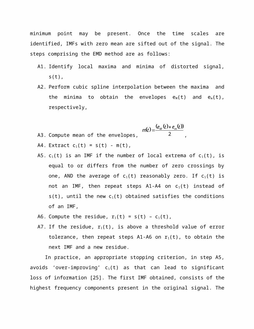
Fig. 19. Response of the method for a voltage fluctuation (Flicker) environment (a) Input signal, (b) Estimated Amplitude

8.12 Comparative Computational Effort

The computational effort between the new approach and the approach presented in [3]

(single rate) is compared in terms of number of multiplication, addition and table search

(functions sin and cos). The total operation number for processing one cycle, i.e. 128 samples, is

presented in TABLE VIII. To obtain these numbers is necessary take into account the down

sampling factor used in TABLE VII and the number of operation in the band-pass filter and EPLL

estimator. Note that the computational effort for the multirate approach is greater than the

approach of [3] only for the number of adds. However, the multirate approach needs only 82%

of multiplies and 7% of table search required for the approach of [3]. It is important to highlight

that the EPLL analyzed in this work did not include the extras filters as proposed in [3] to

smooth the estimates. If these filters were included the computed data in Table II would be still

more favorable to the propose method.

TABLE VIII

number of operations realized within one cycle of fundamental to estimate until 15th HARMONIC

Adds Multiplies Table Search

Single Rate 9600 15360 3840

Multirate 14125 12616 274

8.13 Conclusions

This chapter presents an improved structure of PLL based harmonic estimation [9]. It

has been shown that parameters of a high order harmonic can be extracted performing an

undersampling of this high frequency signal. The frequency estimated is an apparent frequency

that can be converted to its actual value using algebraic relations. The simulations results have

shown that the increase in transitory response was not significant. The computational effort is

reduced compared with [3] and previous structure [9]. Finally, the fact that PLL estimates an

apparent frequency, lower than 240 Hz, makes the implementation in a fixed point DSP-based

system more robust.

8.14 References

[1] M. Karimi-Ghartemani and M. R. Iravani, “A Nonlinear Adaptive Filter for Online Signal

Analysis in Power Systems: Applications,” IEEE Trans. on Power Delivery, vol. 17, no. 2,

pp.617-622, Apr. 2002.

[2] M. Karimi-Ghartemani and M. R. Iravani, “Robust and frequency-adaptive measurement of

peak value,” IEEE Transactions on PowerDelivery, vol. 19, no. 2, pp. 481–489, Apr. 2004.

[3] M. Karimi-Ghartemani and M. R. Iravani, “Measurement of harmonics/inter-harmonics of

time-varying frequencies,” IEEE Transactions on Power Delivery, vol. 20, no. 1, pp. 23–31,

Jan. 2005.

[4] Y. Baghzouz, R. F. Burch, A. Capasso, A. Cavallini, A. E. Emanuel, M. Halpin, A. Imece, A.

Ludbrook, G. Montanari, K. J. Olejniczak, P. Ribeiro, S. Rios-Marcuello, L. Tang, R. Thaliam,

and P. Verde, “Time-varying harmonics: Part I—Characterizing measured data,” IEEE

Transactions on Power Delivery,, vol. 13, pp. 938–944, Jul. 1998.

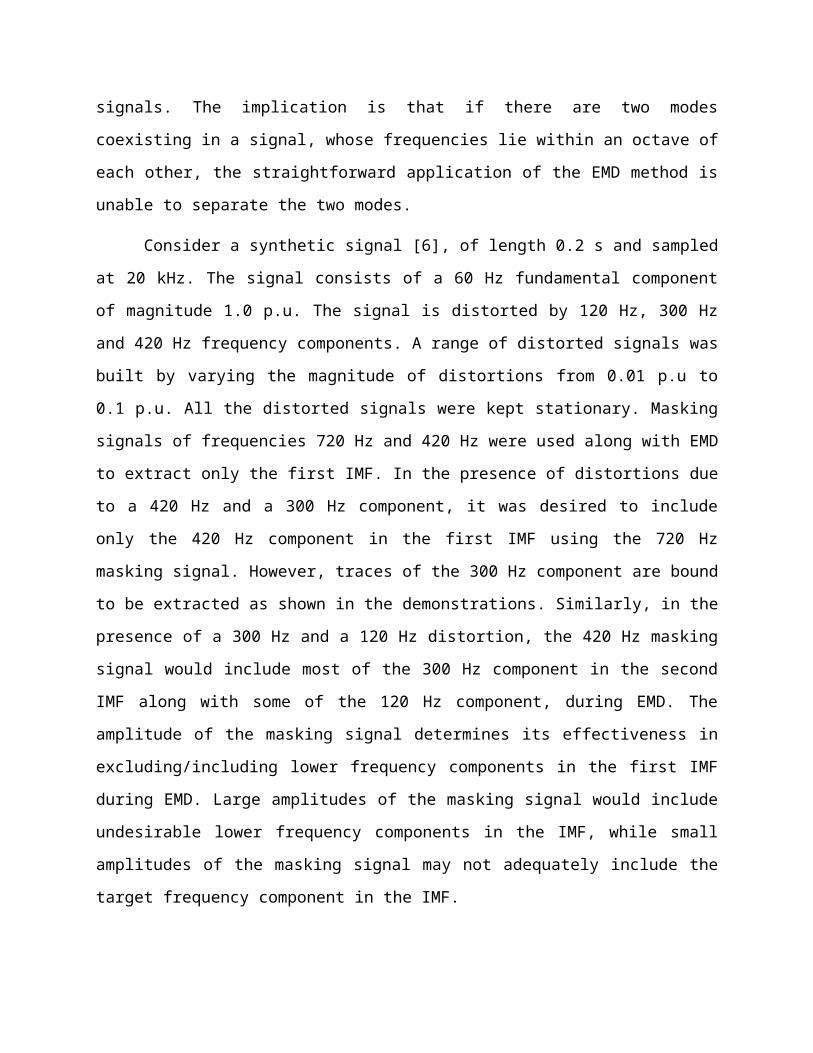
[5] M. V. Chilukuri and P. K. Dash, “Multiresolution S-transform-based fuzzy recognition system

for power quality events,” IEEE Transactions on Power Delivery, vol. 19, no. 1, pp. 323–

329, Jan. 2004.

[6] IEC standard draft 61000-4-7: General guide on harmonics and inter-harmonics

measurements, for power supply systems and equipment connected thereto, Ed. 2000.

[7] D. Gallo, R. Langella and A. Testa, “Desynchronized Processing technique for Harmonic and

interharmonic analysis”, IEEE Trans. Power Del., vol. 19, pp. 993 – 1001, July 2004.

[8] L. L. Lai, C. T. Tse, W. L. Chan, and A. T. P. So, “Real-time frequency and harmonic evaluation

using artificial neural networks,” IEEE Trans.Power Del., vol. 14, pp. 52–59, Jan. 1999.

[9] J. R. Carvalho, P. H. Gomes, C. A. Duque, M. V. Ribeiro, A. S. Cerqueira, and J. Szczupak, “PLL

based harmonic estimation,” Accepted for publication in IEEE PES conference, Tampa,

Florida-USA, 2007

[10] P. P. Vaidyanathan, Multirate Systems and Filter Bank, Englewood Cliffs, New Jersey:

Prentice Hall, 1993, pp. 113, 151-157

[11] S. K. Mitra, Digital Signal Processing: A Computer-based Approach, McGraw-Hill, 3rd ed.,

2006, pp. 383-385, 177, 740

Chapter 9 – Higher Order Statistics for Power Quality Evaluation

Cristiano Augusto G. Marques, Carlos A. Duque, and Moisés V. Ribeiro

9.1 Introduction

The increasing pollution of power line signals and its impact on the quality of power delivery by

electrical utilities to end users are pushing forward the development of signal processing tools

to provide several functionalities, among them it is worth to mentioning the following ones [3]:

i) disturbance detection, ii) disturbance classification, iii) disturbance source identification, iv)

disturbance source localization, v) disturbance transient analysis, vi) fundamental, harmonic,

and interharmonic parameters estimations, vii) disturbance compression, and etc.

Regarding the power quality (PQ) monitoring needs, one can note that the disturbance

detections as well as their start and end points in electric signals is a very important issue for

upcoming generation of equipment for PQ monitoring applications. In fact, nowadays detection

techniques have to present good performance under different sampling rates, frame lengths

ranging from sub-multiples to multiples of power frequency cycle and varying signal to noise

ratio (SNR) conditions. Therefore, for those interested in disturbance analysis, one of the first

and most important part of the whole monitoring equipment and characterization process

refers to the detection task, since it must be performed online and in real-time. Also, it must be

capable of highlighting short and long time disturbances with high detection ratio.

Additionally, it is worth mentioning that equipment for event and variation detections are

required to activate the disturbance tracking so that it can be performed by only processing the

portion of the signal including the target event. As a result, the efficient detection of

disturbances as well as their segmentation in the electric signals allows the efficient use of not

only powerful classification techniques, but also compression, signal decomposition or

representation, parameters estimation, and identification techniques for a comprehensive

analysis of power line signals. The necessity of improved detection performance for the

continuous monitoring of voltage and current signals have motivated the development of

several techniques focusing on a good trade off between computational complexity and

performance. In fact, the correct detection of disturbances in voltage signals, as well as their

start and end points, provide relevant information to characterize the PQ disturbance source,

which is causing the detected disturbance.

The classification or recognition topic is an important issue for the development of the next

generation of PQ monitoring equipment. Basically, it refers to the use of signal processing

based technique to extract as few as possible and, at the same time, representative features

from the power line signals, which are supposed to be voltage and current ones, followed by

the use of a powerful and as simple as possible pattern recognition-based techniques.

This chapter discusses some recent results about the use of higher-order statistics (HOS) [5],[9]

for evaluating the power quality disturbances in electric signals. The majority of techniques for

classification, detection and parameters estimation in power quality application are based on

the use of second-order statistics (SOS). In fact, for a large number of problems based on the

assumption of stationarity of electric signals, the use of SOS is a very interesting solution due to

the good tradeoff between computational complexity and performance. However, if the

stationarity is no longer verified, then the use of HOS can lead to techniques capable of dealing

with the nonstationarity assumption. To verify the effectiveness of HOS for power quality

application, it is shown some recent results when the HOS is applied for the detection of

voltage disturbances in a frame with at lest N=16 samples and for classifying multiple

disturbances in voltage signals. In spite of the increased computational burden, the results

attained with the use of HOS indicate that it can be a powerful tool for the analysis of power

quality disturbances.

9.2 Signal Description

The discrete version of monitored power line signals can be divided into non-overlapped frames

of N samples. The discrete sequence in a frame can be expressed as an additive contribution of

several types of phenomena:

(1)

where n=0,…,N−1, Ts=1/fs is the sampling period, the sequences {f(n)}, {h(n)}, {i(n)}, {t(n)}, and

{v(n)} denote the power supply signal (or fundamental component), harmonics, inter-

harmonics, transient, and background noise, respectively. Each of these signals is defined as

follows:

, (2)

, (3)

, (4)

, (5)

and v(n) is independently and identically distributed (i.i.d.) noise as normal N(0,v2) and

independent of {f(n)}, {h(n)}, {i(n)}, and {t(n)}. In (2), (n), (n), and (n) refer to the

magnitude, fundamental frequency, and phase of the power supply signal, respectively. In (3)

and (4), hm(n) and ij(n) are the mth harmonic and the jth inter-harmonic, respectively, which

are defined as

(6)

and

, (7)

where (n) is the magnitude and (n) is the phase of the mth harmonic. In (7), (n),

(n), and (n) are the magnitude, frequency, and phase of the jth inter-harmonic, respectively.

In (5), (n), (n), and (n) represents impulsive transients named spikes, notches,

decaying oscillations. (n) refers to oscillatory transient named damped exponentials. These

transients are expressed by

, (8)

, (9)

, (10)

and

, (11)

respectively, where and are the nth samples of the ith transient named

impulsive transient or notch. Note that (10) refers to the capacitor switchings as well as signals

resulted from faulted waveforms. Equation (11) defines the decaying exponential as well as

direct current (DC) components ( = 0) generated by geomagnetic disturbances, etc.

The following definition is used in this contribution: i) the vector x=[x(n)…x(n−N+1)]T is

composed of samples from the signal expressed by (1), the vector f=[f(n)…f(n−N+1)]T

constituted by estimated samples of the signal given by (2), the vector h=[h(n)…h(n−N+1)]T is

composed of estimated samples of the signal defined by (3), the vector i=[i(n)…i(n−N+1)]T is

constituted by estimated samples of the signals defined by (4), the vector =[ …

]T is constituted by estimated samples of the signals defined by (8), the vector

=[ … ]T is constituted by estimated samples of the signals defined by (9),

the vector =[ … ]T is composed of estimated samples of the signals

defined by (10), and the vector =[ … ]T is constituted by estimated

samples of the signals defined by (11). v=[v(n)…v(n−N+1)]T is constituted by samples of the

additive noise.

Classification of Single and Multiple disturbances

It is worth mentioning that low-, medium-, and high-voltage electrical networks present

different sets of single and multiple disturbances. As a result, the design of classification

technique for each voltage level has to take into account the information and characteristics of

these networks to attain a high classification performance. For instance, the sets of

disturbances in the high-voltage transmission and low-voltage distribution systems differ

considerably.

The majority of classification techniques developed so far is for single disturbances. For these

techniques, the feature extraction as well as classification techniques have been investigated

and researchers in this field have achieved a great level of development [1],[3]. As a result, the

current classification techniques are capable of classifying single disturbances achieving

classification ratio from 90.00% to 100.00%. Nevertheless, one can note that the incidence of

multiple disturbances, at the same time interval, in electric signals, is an ordinary situation

owing to the presence of several sources of disturbances in the power systems.

Presupposing that electric signals are represented by (1), the recognition of disturbance

patterns composed of multiple disturbances can not be an easy task to be accomplished as in

the case of single disturbance occurrence. In fact, the incidence of more than one disturbance

in the electric signals can lead to techniques attaining reduced classification performance due

to the complexity of classification region if the standard paradigm, which is depicted in Fig. 1, is

considered. It refers to the fact that in the standard paradigm, the feature vector px is extracted

directly from the vector x = f+h+i+timp+tdec+tdam+v and the vector px can be unfavorable for

disturbance classification purpose because the vector x is composed of several components,

which are associated with disjoint disturbances sets. As a result, the design of pattern

recognition technique for classifying multiple disturbances is a very difficult task to be

accomplished.

Figure 1. Standard paradigm for the classification of single and multiple disturbances.

One can state that this is true because the electric signals are in the majority of cases composed

of complex patterns, which is constituted by multiple primitive patterns. Therefore, the surfaces

among the classification regions that are associated with different types of single and multiple

disturbances in the feature vector space, which is defined by the set of feature vectors px, can

be very complex and difficult to attain, even though powerful feature extraction and

classification techniques are applied. As a result, the design of pattern recognition techniques

offer low performance if (1) is composed of multiple disturbances. It indicates that a lot of

efforts have to be put in for the development of powerful pattern recognition techniques

capable of achieving high performance.

To overcome the weakness and reduced performance of the standard paradigm, in the

following a paradigm based on the principle of divider to conquer is presented, which has been

widely and successfully applied to many engineering applications, to design powerful and

efficient disturbance classification techniques for PQ applications. In this paradigm, the vector x

is decomposed into what we call primitive components from which individual disturbances or,

as defined here, primitive patterns can be easily classified. Here, primitive components are

defined as those components from which only single disturbances can be straightforwardly

classified.

It is clear that improved performance can be attained for the classification of single and

multiple disturbances in electric signals, if the electric signals can be decomposed into several

primitive components. By using such a very simple and powerful idea, which is named the

principle of divide to conquer, the design of a very complex classification technique is broken in

several simple ones that can be developed easily. The result derived from this paradigm is very

interesting because the incidence of several sets of classes of disturbances can be identified

easily. In fact, each of the vectors f, h, i, timp, tnot, tdec, and tdam are related to disjointed

classes of disturbances and their recognition in parallel can be performed easily.

From a PQ perspective, the advantages and opportunities offered by this paradigm is very

appealing and promising to completely characterize the behavior of electric signals not only for

classification purpose, but also for other very demanding issues listed at the beginning of next

Section. To make this strategy successful, one has to develop signal processing techniques

capable of decomposing the vector x into the vectors f , h, i, timp, fnot, tdec, and tdam to allow

the further extraction of simple and powerful feature extraction and the use of simple

classifiers.

This is a very hard and difficult problem to be solved so that it should be deeply investigated by

signal processing researchers interested in this field. In fact, the decomposition of vector x into

the vectors f, h, i, timp, tnot, tdec, and tdam is not a simple task to be accomplished with simple

signal processing techniques. However, if one assumes that the vector x is given by

(12)

where and (13)

Then some signal processing techniques can be applied to decompose x into the vectors f, h,

and u. And, as a result, high-performance pattern recognition technique for a limited and very

representative set of disturbances in electric signals can be designed. In fact, the decomposition

of the vector x into the vectors f, h, and u allows one to design classification techniques for

disjoint sets of disturbances associated with the primitive components named fundamental,

harmonic, and transient, respectively. The scheme of the proposed technique, which was

introduced in [1], is portrayed in Fig. 2.

Figure 2. Scheme of proposed technique for the classification of single and multiple

disturbances.

In the proposed technique, the signal processing block implement notch filters or narrow pass-

band filter to decompose x into the vectors f, h, and u. Thereafter, HOS-based features, which

were previously selected, are extracted and, then Bayesian classifiers area applied.

From the vector f, four disjoint patterns of disturbances, which are named sag, swell, normal,

and interruption, are primitive patterns. If one considers the vector h, then one primitive

pattern called harmonic is defined. Finally, for the vector u, it is well known that at least five

disturbances or primitive patterns (inter-harmonics, spikes, notches, decaying oscillations, and

damped exponentials) can occur simultaneously in the vector u. As a result, 25=32 classes of

disturbances can be associated with the vector u and a very complex hypotheses test should be

formulated.

While the design of pattern classifiers to work with the feature vectors extracted from vectors f

and h are quite simple, the design of those techniques for disturbances classification in the

vector u could be a very hard task to be accomplished. However, it is worth stating that the

difficulties associated with the proposed scheme are lower than the ones associated with

standard scheme, which is illustrated in Fig. 1.

Detection of Disturbances

As far as disturbance detection is concerned, an important issue that comes to our attention is

the fact that all detection techniques presented so far do not address the problem of the

minimum number of samples, Nmim, needed to detect the occurrence of disturbances. In fact,

the development of a new technique based on this premise is interesting, because for a given

Nmim such technique can be designed to achieve high detection rate of disturbances in voltage

signals. Then, an appropriate sampling rate, fs, that will guarantee the detection of

disturbances in frames with lengths corresponding to multiples or sub-multiples of one-cycle of

the fundamental component can be successfully applied.

Usually, the detection of disturbances or events in the vector x can be formulated as the

decision between two hypothesis

, (14)

where hypothesis refers to normal conditions of voltage signals and hypothesis is

related to abnormal conditions in voltage signals. In (14), the vector ∆f represents a sudden

variation in the fundamental component and the vector f denotes the steady-state component

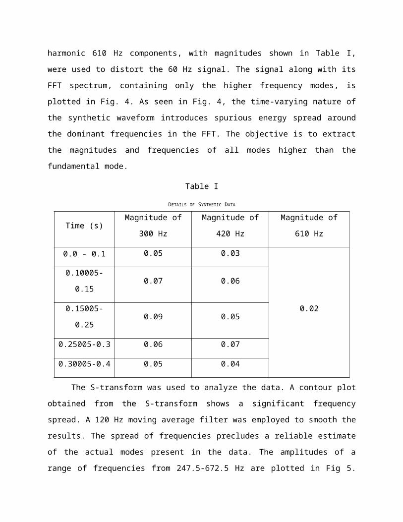
of the fundamental component, whose samples as given by (2). Finally, the vector u refers to

the occurrence of disturbance in the voltage signals resulted from different sources that do not

appear in the fundamental component.

Supposing that L is the length of the disturbance and N>L, it can be written that x = f+∆f+u+v =

[x(n)...x(n−N+1)]T , u+∆f = [0Td,(u+∆f )TL, 0TN−L−d]T , (u+∆f )L =[u(n+d)+

∆f(n+d)...u(n−N+1+L+d)+ ∆f(n−N+1+L+d)]T is the disturbance signal samples vector. 0Tm is a

column vector with m elements equal to zero. d and d+L are start and end points of the

disturbance in the N-length frame.

Based on this formulation, the disturbance occurrence interval is denoted by

(15)

where (n) is the unit step function. The disturbance detection process involves several

variables that depend on the kind of application. For instance, the starting point d could be

known or not; the duration L could be available or not; the wave shape of the disturbance u can

be known, partially known, or completely unknown [2]. In this context, is a simple

hypothesis and is a composite hypothesis.

From the detection theory, it is known that if the background noise v(n) is additive, i.i.d., and

presents a Gaussian distribution with known parameters, then the generalized likelihood ratio

test (GLRT) is the classical process which assumes the form of a matched filter. However the use

of such techniques demands high computational complexity. It is worth mention that if the

background noise v(n) is not Gaussian then the implementation of the GLRT presents a

considerable computational burden for even off-line applications.

Analyzing the vector v, it is noted that this signal usually is modeled as a i.i.d. random process in

which the elements present a Gaussian probability density function (p.d.f.). Therefore, the use

of 2nd-order statistics to analyze the occurrence of disturbances can severely degrade the

detection performance if the power of vector v is high. Another very important concern resides

on the fact that the vector v neither is an i.i.d. random process nor a Gaussian one, then the use

of 2nd-order statistics can be very unreliable to extract qualitative information for detection

purpose if the power of the Gaussian noise is high.

On the other hand, the use of HOS based on cumulants appears to be a very promising

approach for disturbance detection in voltage signals because it is more appropriate for dealing

with no-Gaussian signals. In fact, the cumulants are blind to any kind of Gaussian process,

whereas 2nd-order information is not. Then, cumulant-based signal processing methods can

handle colored Gaussian noise automatically, whereas 2nd-order methods may not. Note the

vector v can be modeled as a colored Gaussian noise. Therefore, cumulant-based methods

boost signal-to-noise ratio when signals are corrupted by Gaussian measurement noise [9].

Additionally, the cumulants of higher-order statistics provide more relevant information from

the random process. The use of such relevant information for detection purpose in (12) and

other applications such as parameters estimation and classification have been applied in several

applications which are not related to power systems. Based on this discussion and assuming

that f and u carry out relevant information from the disturbance occurrence, then the

hypothesis stated in (14) is here reformulated as follows:

; (16)

where v= + . The hypothesis formulation introduced in (16) emphasizes the need to

analyze abnormal events in the two major components of voltage signals represented by the

vectors f and u to detect occurrences of disturbances. While hypotheses and are related

to normal conditions of such voltage signal components, hypotheses and refer to

abnormal conditions in these components.

Equation (16) means that one looks for some kind of abnormal behavior in one or two

individual components of x to make a decision about disturbance occurrences. This concept is

very attractive, because the vectors f+∆f+ and h+i+t+ can reveal insightful and different

information from the voltage signals. These information not only leads to efficient and simple

detection technique, but also contribute to the development of very promising compression,

classification, and identification techniques for PQ applications [1].

Fig. 3 presents the scheme of a detection technique that makes use of (16). This technique was

introduced in [2]. In this technique, a notch or bandpass filter is use to decompose the vector x

into u and f+∆f vectors. Then, features based on HOS, which was previously selected, are

extracted from the vectors u and f+∆f. After that, a Bayesian classifier is applied to verify the

occurrence of disturbance in the vector x.

Figure 3. Block diagram of the detection method of abnormal conditions.

We call attention to the fact that the technique discussed in this section allows detection ratios

very close to 100 % if SNR is higher than 25 dB and the minimum number of samples in a frame

length is higher than 16, as it is verified in the result Section. As a result, this technique can be

applied to detect a large number of disturbances ranging from variations to high frequency

content events if a appropriate sampling rate is considered. For example, if the sampling rate is

equal to fs = 32×60 Hz, then this technique provide a high detection ratio if frame length

corresponding at least a half cycle of the fundamental component is considered. In the case the

sampling rate is fs = 512×60 Hz, similar detection performance is attained with a frame length

corresponding at least 1/32 cycles of the fundamental component. One can note that if this

technique is well designed to a target sampling rate, then it is capable of detecting disturbances

in a very short time interval corresponding sub-multiples of the one cycle of the fundamental

component.

Note that the disturbance detection in a frame with length longer than one-cycle is not a

novelty, but can be performed very well with the detection technique and, as consequence, an

improved performance of the proposed technique under more severe conditions.

The novelty offered by this technique is to provide a high detection ratio when the frame

lengths are sub-multiples of one cycle of the fundamental component. Note that the detection

capacity of this technique is improved if frame lengths corresponding more than one cycle of

the fundamental component are used, because the use of a large number of samples allows a

better estimation of the HOS-based parameters.

By using the proposed technique, one is able to design source identification and disturbance

classification techniques that can use the transient behavior associated with the detected

disturbances to classify the disturbances and to identify the possible disturbance sources for

the ongoing disturbance in short-time intervals.

HOS Features

As stated in [4]: Feature extraction methods determine an appropriate subspace of

dimensionality m (either in a linear or a nonlinear way) in the original feature space of

dimensionality d. Linear transforms, such as principal component analysis, factor analysis, linear

discriminant analysis, and projection pursuit have been widely used in pattern recognition for

feature extraction and dimensionality reduction.

Despite the good performance achieved by these mentioned feature extraction techniques, it

has been recently recognized that HOS-based techniques are promising approaches for features

extraction if the patterns are modeled as non-Gaussian processes. Analyzing vectors f, h, and u,

one should note that these random vectors usually are modeled as a i.i.d. random processes in

which the elements present a nonGaussian probability mass function (p.m.f.). The cumulants of

higher-order statistics provide much more relevant information from the random processes.

Besides that, the cumulants are blind to any kind of Gaussian process, whereas 2nd-order

information is not. Then, cumulant-based signal processing methods can handle colored

Gaussian noise automatically, whereas 2nd-order methods may not. Therefore, cumulant-

based methods boost signal-to-noise ratio when signals are corrupted by Gaussian

measurement noise and can capture more information from the random vectors [5],[9].

Remarkable results regarding detection, classification, and system identification with cumulant-

based methods have been reported in [5],[9].

By setting the lag = i, i=1,2,3,..., the expressions of the diagonal slice of second-, third-, and

fourth- order cumulant elements of a zero mean and stationary random vector z, which is

assumed to be one of the vectors f−E{f}, h−E{h}, and u−E{u}, are expressed by [5]

, (17)

(18)

and

, (19)

respectively, where i is the ith lag. Assuming that z is a N-length vector, the standard

approximation of (17)-(19) are expressed by

(20)

(21)

and

(22)

respectively, where i =0,1,2,…,N/2−1. We argue that the standard approximation to extract

HOS-based features is not appropriate if the frame length is short. As a result, a high sampling

rate or a long frame length has to be taken into account to extract representative HOS-based

features.

Due to the limitation of (20)-(22) to estimate the HOS-based features and based on the fact that

the electric signals can be seen as cyclic or/and quasi-cyclic ones, we proposed in [1]-[2] the use

of this information to define other approximation of HOS parameters. By using this information

into (17)-(19), the new approximation for the HOS-based feature extractions can be expressed

as follows:

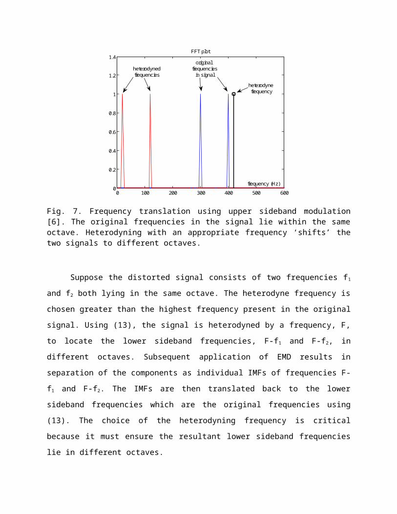
(23)

(24)

(25)

where i=0, 1 ,2 ,…, N −1 and mod (a,b) is the modulus operator, which is defined as the

remainder obtained from dividing a by b. The approximations presented in (23)-(25) lead to a

very interesting result where one has a shortened finite-length vector from which HOS-based

parameters have to be extracted. The use of mod (.) operator means that we are assuming that

the vector z is a N-length cyclic vector. The reason for this refers to the fact that by using such

very simple assumption we can evaluate the approximation of HOS-based parameters with all

available N samples. Therefore, a reduced sampling rate and/or a shortened frame-length could

be valuable for HOS parameters estimation. That is one of the reasons for the improved

performance achieved by the proposed technique in Result Section.

Now, suppose that the elements of the vector z = [z(0), z(1),…,z(N−1)]T are organized from the

smallest to the largest values and the vector composed of these values are expressed by zor =

[zor (0), zor (1), · · · , zor (N −1)]T, where zor (0) ≤ zor (1) ≤,…,≤ zor (N −1). If one replaces the

vector z by the vector zor in (20)-(25), then the extracted cumulants are named ordered HOS-

based features. By doing so, the set of HOS-based features is composed of several elements.

The HOS-based feature vector, whose elements are candidates for use in the proposed

classification technique, extracted from the vectors z and zor, is is given by

(26)

where z denotes f , h, and u, i = 1 refers to a normal condition of voltage signals, i = 2 denotes

the incidence of single or multiple disturbances in the vector z if the aim is classification. On the

other hand, if the purpose is detection, then z denotes f and u, i = 1 refers to a normal condition

of voltage signals, i = 2 denotes the abnormal one. Note that

(27)

and

(28)

where

(29)

(30)

(31)

and

(32)

where j = 2, 3, 4. Now, to select a valuable set of features, it is demanded the use of a feature

selection technique. The need for the use of feature selection technique in the set of features

extracted from voltage and current signals is due to the fact that the feature set is very large.

Aiming at the choice of a representative, finite, and reduced set of features from power line

signals that provides a good separation among distinct classification regions associated with all

primitive patterns, the use of the Fisher’s discriminant ratio (FDR) is applied [4].

The reason for using the FDR and not other feature selection technique such as sequential

forward floating search (SFFS) or sequential backward floating search (SBFS) is that the FDR

technique presented good results for this application. The FDR vector which leads to a

separation in a low-dimensional space between sets of feature vectors associated with different

primitive patterns is given by

(33)

where Jc = [J1 · · · JLl]T , Ll is the total number of features, m1 and m2, and D21 and D22 are the

means and variances vectors of parameters vectors p1,k, k =1, 2, …, Mp and p2,k, k =1, 2, …,

Mp. p1,k and p2,k are feature vectors extracted from the kth voltage signals with and without

disturbances and Mp denotes the total number of feature vectors for the classes of

disturbances associated with the presence or not of disturbances. The symbol refers to the

Hadarmard product r s = [r0s0 r1s1…rLr−1sLr−1]T . The ith element of the FDR vector, see (17),

having the highest value, Jc(i), is selected for use in the classification technique. Applying the

same procedure, K features associated with the K highest FDR values are selected.

Numerical Results

The performance of both classification and detection techniques that were introduced in [1]-[2]

and briefly discussed in previous Sections are presented below.

Performance of the Classification Technique

To verify the performance of the proposed technique to classify disturbances in the vectors f ,

h, and u, simulations were carried out with several waveforms of voltage signals generated with

a sampling rate equal to fs = 256×60 samples per second (sps) and 32 bits for amplitude

quantization. The selected primitive patterns are sag, swell, interruption, harmonic, impulsive

transient, notch, and damped oscillation.

Figs. 4-6 portray the selected features extracted from vector f by using the FDR to verify the

occurrence of interruptions, sags, and swell. In these plots, the symbols * and o are associated

with the occurrence or not of each disturbance in the test data. One can note that there are

linear separations, then the Bayesian classifiers reduces to a linear ones.

Tab. I lists the attained classification ratio with the proposed technique applied to classify the

set of primitive patterns (sag, swell, and interruption) that are associated with the vector f.

Fig. 4. HOS-based features extracted from vector f for interruption 1= (68).

Fig. 5. HOS-based features extracted from vector f for sag 1= (512) and 2= (194).

Fig. 6. HOS-based features extracted from vector f for swell 1= (191).

TABLE I

PERFORMANCE OF THE PROPOSED TECHNIQUE TO CLASSIFY

DISTURBANCES IN THE VECTOR f.

Frame Length Interruption (CR in

%)

Sag (CR in %) Swell (CR in %)

1C 99.93 99.95 100.00

2C 99.96 99.97 100.00

3C 100.00 99.98 100.00

4C 100.00 100.00 100.00

The following considerations were taken into account for the simulations: i) N =128, 256, 512,

768, and 1024, then the lengths of the vector f correspond to 1/2, 1, 2, 3 and 4 cycles of the

fundamental component; ii) feature vector pf with four HOS-based features, which were

previously selected with the FDR technique, for each primitive pattern; iii) two thousand sets of

primitive patterns generated and equally divided into training and test data; iv) the use of Bayes

detection technique based on the maximum likelihood (ML) criterion; v) variance of Gaussian

noise equal to −30 dB; vi) the amplitude of the fundamental component, A0, assumes values to

characterize the disturbances in accord with the IEEE 1159-1995 Standard [50] and the phase,

0, is modeled as uniform random variable in the interval (0, 2]; viii) the pre-processing block

was implemented with finite word-length with 16 bits.

From the results listed in Tab. I, one notes that the proposed technique achieves good

performance. In Tab. I, C means cycles of the fundamental component and CR refers to the

classification ratio in percentage. The improvements shown here refer to the attained CR=100%

if the lengths of vector f correspond to 1, 2, 3 and 4 cycles of the fundamental component. In

the previously developed methods, the results are reported when N ≥ 1024 or, at least, 4 cycles

of the fundamental component, see [1].

The numerical analysis of the proposed technique for the classification of primitive pattern in

voltage signals named harmonic was carried out by taking into account the following

considerations: i) N =128, 256, 512, 768, and 1024 and, consequently, the lengths of the vector

h correspond to 1, 2, 3 and 4 cycles of the fundamental component; ii) two thousand sets of

harmonic disturbances equally divided in training and test patterns were considered; iii) Bayes

detection technique based on the ML criterion was designed; iv) variance of the Gaussian noise

is equal to −30 dB; iv) the harmonic components, whose frequency are m=0, m = 3, 5, 7, 9, 11,

13, and 15, have amplitudes Ai and i modeled as uniform random variables in the intervals

(0.01,0.4] and (0,2], respectively; v) feature vector ph composed of one element selected by

FDR criterion. The generated harmonics comply with the IEEE 1159-1995 standard [7].

Fig. 7 shows the selected HOS-feature obtained from vector h to detect harmonic presence. The

symbols * and o are associated with the occurrence or not of harmonic in the test data,

respectively.

Fig. 7. HOS-based features extracted from h, 1= .

The results achieved with the proposed technique are presented in Tab. II. The CR as high as

100% is not novel if N ≥ 1024 or, at least, 4 cycles of the fundamental component is taken into

account [1]. The novelty here is the fact that the proposed technique is capable of achieving CR

as high as 100% if the length of vector h corresponds to 1/2, 1, 2, 3 and 4 cycles of the

fundamental component.

TABLE II

PERFORMANCE OF THE PROPOSED TECHNIQUE FOR HARMONIC CLASSIFICATION

Frame Length CR in %

1/2 C 100.00

1C 100.00

2C 100.00

3C 100.00

4C 100.00

To check the effectiveness of the proposed technique for the classification of primitive patterns

in the vector u, the following considerations were taken into account; i) N=1024, which

corresponds to four cycles of the fundamental component; ii) four-length feature vector pu in

which all elements are selected with the FDR technique; iii) 3000 sets of disturbances such as

impulsive transients, notches, and damped oscillations equally divided into training and test

data; iv) Bayes detection technique based on the ML criterion; v) additive noise power is equal

−30 dB; and vi) single incidence of disturbances in the vector x that appears in the primitive

component represented by the vector u.

Figs. 8-10 depict the selected HOS-based features that were extracted from vector u to classify

the disturbances as oscillatory transient (damped oscillations), impulsive transient and notch. In

these figures, the symbols * and o are associated with the occurrence or not of each

disturbance in the test data.

The attained results with the test data are shown in Tab. III. One can note that the proposed

technique is capable of classifying almost all primitive patterns in the vector u.

TABLE III

PERFORMANCE OF THE PROPOSED TECHNIQUE FOR DISTURBANCE CLASSIFICATION

IN THE VECTOR u WHEN N=1024 IS CONSIDERED.

Disturbance CR in %

Notch 100.00

Impulsive transient 100.00

Oscillatory transient (damped

oscillation)

100.00

Fig. 8. HOS-based features extracted from u to classify the oscillatory transient named damped

oscillation. 1 = (257).

Fig. 9. HOS-based features extracted from u to classify the impulsive transient 1= (4) and

2 = (511).

Fig. 10. HOS-based features extracted from u to classify the notch disturbance 1= (97).

Tab. IV presents the performance of the proposed technique applied to classify multiple

primitive patterns. Here, it is considered N=1024. In Tab. IV, the term Transient refers to notch,

spike or damped oscillation, the term Fund denotes disturbances in the fundamental

component, the term Harm refers to the harmonic disturbance, and the term Two transients

and Three Transients mean that two or three distinct transients occur at the same frame,

respectively. From Tab. IV, one verifies that the proposed technique is capable of classifying

several sets of multiple primitive patterns in voltage signals.

TABLE IV

PERFORMANCE OF THE PROPOSED TECHNIQUE FOR THE CLASSIFICATION

OF MULTIPLE DISTURBANCES IN VECTOR x.

Disturbances CR in %

Fund + Harm 100.00

Fund + Harm + One transients 99.98

Fund + Harm + Two transients 98.35

Fund + Harm + Three transients 96.89

Finally, the proposed technique is compared against a previous technique recently introduced

in [8]. A set of disturbances, defined in accordance with [8] was generated. By using this set of

disturbances, a performance comparison between the technique presented in [8] and the one

introduced in [1] are comparatively reported in Tab. V. Based on the reported results, one can

verify that the technique introduced in [1] not only surpasses the performance of the previous

one, but it also shows a considerable improvement.

TABLE V

PERFORMANCE COMPARISION IN TERMS OF CLASSIFICATION RATIO (%) ACHIEVED BY

PROPOSED TECHNIQUE AND THE TECHNIQUE PROPOSED IN [8].

Class Proposed Technique Technique proposed in [8]

C1 100.00 100.00

C2 100.00 100.00

C3 100.00 85.55

C4 100.00 100.00

C5 100.00 82.00

C6 100.00 96.50

C7 100.00 100.00

One has to note that the results reported were obtained with disturbances synthetically

generated. As a result, the proposed technique will show degradation in its performance if it is

applied to real voltage signals, but it is worth stating that the classification technique proposed

in [8] will present similar behavior. At this point we are not able to say, under this situation,

what technique will present the lowest degradation.

Performance of the Detection Technique

To evaluate the performance of the proposed technique, several waveforms of voltage signals

were synthetically generated. The generated disturbances are sags, swells, interruptions,

harmonics, damped oscillations, notches, and spikes. The sampling rate considered was fs =

256×60 samples per second (sps). Simulation with other sampling rates were performed, but

will not be presented here for the sake of simplicity.

However, it is worth pointing that similar performance of the proposed technique is verified

when fs = 32 × 60 Hz, fs = 64 × 60 Hz, fs = 128 × 60 Hz, fs = 512 × 60 Hz, fs = 1024 × 60 Hz, and fs

= 2048 × 60 Hz if we take into account N ≥ 16. For the notch filter factor equal 0.997.

Also, the detection performance of the proposed technique is verified with measurement data

of voltage signals available from IEEE working group P1159.3 website, which focused on data

file format for power quality data interchange. The available voltage measurement were

obtained with fs =256×60 Hz. The SNR of these data is around 40 dB. For the sake of simplicity,

the proposed technique is named HOS, the techniques introduced in [10] are named RMS 1 and

RMS 2. RMS 1 and RMS 2 refer to the detection techniques based on the rms evaluation with a

half and one cycles of the fundamental component, respectively.

Fig. 11 gives a picture of the performance of the HOS, RMS 1, and RMS 2 techniques when fs =

256 × 60 Hz and N = 256, 128, 64, 32, and 16. These used frame lengths correspond to 1, 1/2,

1/4, 1/8, and 1/16 cycles of the fundamental component, respectively. To obtain these results,

2236 synthetic waveforms of voltage signals were generated. The synthetic voltage

disturbances generated are sags, swells, interruptions, harmonics, damped oscillations,

notches, and spikes. Although in measurement data we can see that the SNR is around 40 dB,

we evaluated the performance of the three detection techniques for the SNR ranging from 5 up

to 30 dB, but, for the sake of simplicity, only the results achieved when SNR=30 dB is presented.

From this plot, one can see that HOS technique performance provides the lowest error

detection ratio.

Fig. 11. Error detection ratio when the frame lengths correspond to 1/16, 1/8, 1/4, 1/2 and 1

cycles of the fundamental component.

Fig. 12 shows the results achieved when sags, swells, and interruptions occur in the voltage

signals to illustrate the performance of all techniques when typical disturbances associated with

the fundamental components occur. The frame lengths correspond to 1, 1/2, 1/4, 1/8, and 1/16

cycles of the fundamental component and the number of synthetic waveform is equal to 880.

One can note that the performance difference among HOS, RMS 1 and RMS 2 techniques is

considerably reduced. It is something expected because RMS 1 and RMS 2 techniques were

developed to detect sag disturbances as well as their sources. Based on other simulation

results, one can state that if the disturbance set is reduced to be composed of voltage sags,

then the performance of the HOS technique is slightly better than the performance of RMS 1

and RMS 2 techniques if SNR is higher than 25 dB and much better if the SNR is lower than 25

dB.

From the results portrayed in Figs. 11 and 12, one can note that the proposed technique offers

a considerable enhancement compared with the previous ones. In fact, the use of information

from both fundamental and transient components provides more relevant characterization of

disturbances in voltage signals, especially when N is reduced.

Fig. 12. Error detection ratio when the frame lengths are 1/16, 1/8, 1/4, 1/2 and 1 cycles of the

fundamental component.

The results obtained with HOS, RMS 1, and RMS 2 techniques when the SNR varies between 5

and 30 dB is highlighted in Fig. 13. The following assumptions were made to carry out the

simulation: i) the frame length is equal to 1 cycle of the fundamental component, ii) fs = 256 ×

60 Hz, iii) the generated synthetic voltage disturbances are sags, swells, interruptions,

harmonics, damped oscillations, notches, and spikes, iv) the number of data is 2236 .The results

verify that HOS technique presents an improved performance when the SNR is higher than 10

dB.

Fig. 14 shows the performance of all three detection techniques when the measurement data

of the IEEE working group P1159.3 are used. This database is comprised of isolated and multiple

events. The HOS, RMS 1, and RMS 2 techniques were designed with real data in which the SNR

is equal 40 dB. The generated voltage disturbances are sags, swells, interruptions, harmonics,

damped oscillations, notches, and spikes. And, the number of data for design and test are equal

to 2236 and 110, respectively. It is clear to note that the HOS technique is capable of detecting

all disturbances, but the same is not possible with the RMS 1 and RMS 2 techniques.

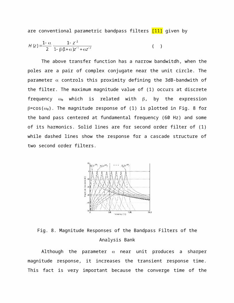
Fig. 13. Error detection ratio when the frame length is equal to 1 cycles of the fundamental

component and the SNR ranges from 5 up to 30 dB.

Fig. 14. Error detection ratio when the measurement data from IEEE working group P1159.3 is

considered. The frame lengths are equal to 1/16, 1/8, 1/4, 1/2 and 1 cycles of the fundamental

component and the SNR is around 40 dB.

The performance of the HOS technique when the SNR ranges from 5 up to 30 dB and the frame

lengths correspond to 1, 1/2, 1/4, 1/8, and 1/16 cycles of the fundamental component is

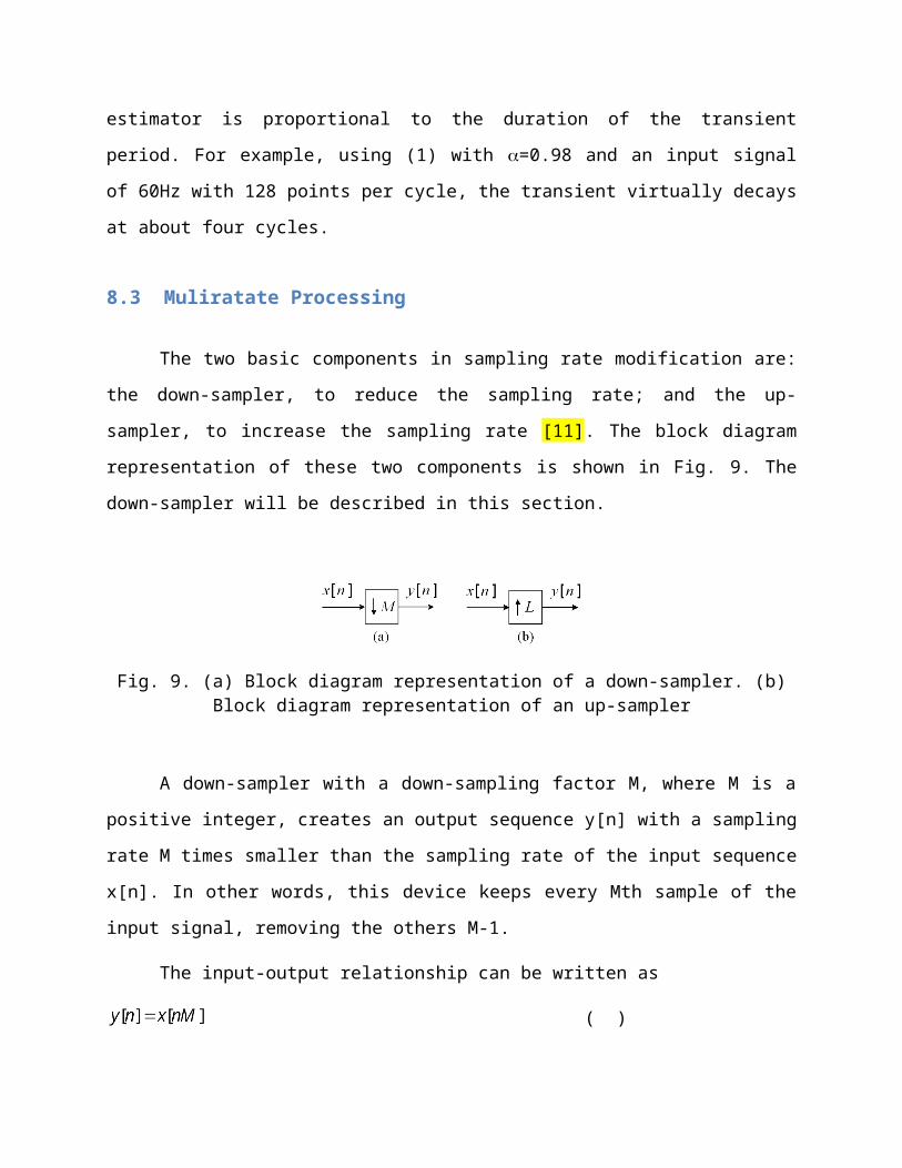
depicted in Fig. 15. One can note that the performance of the HOS-based technique achieves

expressive detection ratio when the SNR is higher than 25 dB.

Fig. 15. Error detection ratio attained by HOS when the frame length is equal to 1/16, 1/8, 1/4,

1/2 and 1 cycles of the fundamental component and the SNR ranges from 5 up to 30 dB.

Overall, from the results obtained, it is seen that the proposed technique is more effective in

terms of performance than the technique introduced in [10], if a reduced-length vector x is

considered for detecting abnormal conditions of voltage signals.

Concluding Remarks

This contribution discussed the use of HOS for the analysis of power quality disturbances.

Recent techniques for detection and classification of disturbances in voltage signals were

presented. From the numerical results obtained with both techniques, one can note that HOS

can be a powerful tool for power quality applications.

References

[1] M. V. Ribeiro and J. L. R. Pereira, “Classification of single and multiple disturbances in

electric signals,” EURASIP Journal on Advanced Signal Processing, Special Issue on Emerging

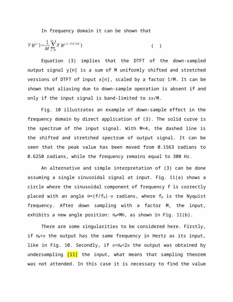
Signal Processing Techniques for Power Quality Applications, vol. 2007, 18 pages, Article ID

56918, 2007.

[2] M. V. Ribeiro, C. A. G. Marques, A. S. Cerquiera, C. A. Duque, and J. L. R. Pereira, “Detection

of disturbances in voltage signals for power quality analysis using HOS,” EURASIP Journal on

Advanced Signal Processing, Special Issue on Emerging Signal Processing Techniques for Power

Quality Applications, vol. 2007, 18 pages, Article ID 59786, 2007.

[3] M. V. Ribeiro, Signal processing techniques for power line communication and power quality

applications, Ph.D. Dissertation, University of Campinas (UNICAMP), Apr. 2005, in Portuguese.

[4] A. K. Jain, R. P. W. Duin, and J. Mao, “Statistical pattern recognition: A Review,” IEEE Trans.

on Pattern Analysis and Machine Intelligence, vol. 22, no. 1, pp. 4–37, 2000.

[5] J. M. Mendel, “Tutorial on higher-order statistics (spectra) in signal processing and system

theory: theoretical results and some applications,,” Proc. of the IEEE, vol. 79, no. 3, pp. 278–

305, Mar. 1991.

[6] I. Y. H. Gu, N. Ernberg, E. Styvaktakis, and M. H. J. Bollen, “A statistical-based sequential

method for fast online detection of faultinduced voltage dips,” IEEE Trans. on Power Delivery,

vol. 19, no. 2, pp. 497–504, 2004.

[7] IEEE 1159 Working Group, “IEEE 1159-1995 recommended practice on monitoring electrical

power quality,” Nov. 1995.

[8] H. He and J. A. Starzyk, “A Self-organizing learning array system for power quality

classification Based on Wavelet Transform,” IEEE Trans. on Power Delivery, vol. 21, no. 1, pp.

286–295, Jan. 2006.

[9] C. Nikias and A. P. Petropulu, Higher-order spectra analysis, 1st Ed. Prentice Hall, 1998.

[10] I. Y. H. Gu,N. Ernberg, E. Styvaktakis, and M. H. J. Bollen, “A statistical-based sequential

method for fast online detection of fault-induced voltage dips,” IEEE Transactions on Power

Delivery, vol. 19, no. 2, pp. 497–504, 2004.

Chapter 10 - Interharmonic Components Generated by Adjustable

Speed Drives

Francesco De Rosa, Roberto Langella, Adolfo Sollazzo and Alfredo Testa

10.1 Introduction

Adjustable Speed Drives (ASDs) based on double stage conversion systems generate

interharmonic current components in the supply system side, the DC link and output side, in

addition to harmonics typical for single stage converters [1]-[4]. Under ideal supply conditions,

interharmonics are generated by the interaction between the two conversion systems through

the intermodulation of their harmonics [5]. When unbalances, background harmonic and

interharmonic distortion are present in supply voltages more complex intermodulation

phenomenons take place [6].

To characterize the aforementioned process, the interharmonic amplitudes (and

phases), frequencies and origins have to be considered. The interharmonic amplitude

importance for compatibility problems is evident: a comprehensive simulation or analysis for

each working point of the ASD is needed and proper deterministic or probabilistic models must

be used in accordance with the aim of the analysis. Various models are available: experimental

analogue, time domain and frequency domain models [7]- [11]. Each of them is characterized

by a different degree of complexity in representing the AC supply-system, the converters, the

DC link and the AC supplied system. Whichever is the model, particular attention must be

devoted to the problem of the frequency resolution and of the computational burden [12].

As for the interharmonic frequencies, whichever is the kind of analysis to be performed,

it is very important to forecast them, for a given working point of the ASD. This allows

evaluating in advance the Fourier fundamental frequency that is the maximum common divisor

of all the component frequencies that are present and gives the exact periodicity of the

distorted waveform. Other reasons are related to the effects of interharmonics such as light

flicker, asynchronous motor aging, dormant resonance excitation, etc. The frequency forecast

requires: i) in ideal supply conditions, only the study of the interactions between rectifier and

inverter, which are internal to the ASD; ii) when unbalances and/or background harmonic and

interharmonic distortion are present in supply voltages, also the study of the further

interactions between the supply system and the whole ASD.

As for the origins of a given interharmonic, the availability of a proper symbolism for

interharmonic turns out to be very useful. In fact, while the frequency is a sufficient information

to find out the origin of harmonic components (in a defined scenario or conversion system), the

same is not true for interharmonic components. These components have frequencies which

vary within a wide range, according to the output frequency, and can assume harmonic

frequencies or even become DC components. Moreover, they overlap in situations in which two

or more components of different origin assume the same frequency value. In general, the

presence of non ideal supply conditions makes impossible to recognize the origins without

complex analyses. Anyway, the knowledge of the normal ASD behaviour in ideal conditions may

help in recognizing what derives from the ASD internal behaviour and what from interactions

with non ideal supply system.

In this chapter, reference is made to ideal supply conditions which allow recognising the

frequencies and the origins of those interharmonics which are generated by the interaction

between the rectifier and the inverter inside the ASD. Formulas to forecast the interharmonic

component frequencies are developed firstly for LCI drives and, then, for synchronous

sinusoidal PWM drives. Afterwards, a proper symbolism is proposed to make it possible to

recognize the interharmonic origins. Finally, numerical analyses, performed for both ASDs

considered in a wide range of output frequencies, give a comprehensive insight in the complex

behaviour of interharmonic component frequencies; also some characteristic aspects, such as

the degeneration in harmonics or the overlapping of an interharmonic couple of different

origins, are described.

10.2 Harmonics and Interharmonics in LCI Drives

LCI drives are still largely used in high power applications. In this type of ASDs the DC-

link is made up of an inductor according to the typical scheme shown in Fig. 1.

Fig. 1. LCI drive scheme.

In the following, formulas for the evaluation of harmonic and interharmonic frequencies

of the DC-link (dc), supply system (ss) and output side (os) currents are reported. The formulas

are obtained applying the principle of modulation theory fully developed in [1], [2] and [6] and

summarised in Appendix A. The majority of the symbols in the following sections are defined in

the Nomenclature.

DC-LinkThe harmonics due to both the rectifier and the inverter are present in idc(t). Their

frequencies are, respectively:

v=1,2,3,…. (1)

j=1,2,3,…. (2)

being hssdc and hos

dc the order of the DC-link harmonic due to the supply side rectifier and to the

output side inverter.

The interharmonics due to the intermodulation operated by the two converters are also

present [8]. Their frequencies are:

v=1,2,3, j= 1,2,3,…. (3)

where the absolute value, here and in the following formulas, is justified by the symmetry

properties of the Fourier Transform [16]. Each couple of rectifier () and inverter (j) harmonics

produces a corresponding interharmonic frequency. In general, two or more couples (j) may

give even the same values of interharmonic frequencies.

10.3 Supply System Side

The harmonic frequencies of iss(t) derive from the modulation of the DC component and of the

components (1) of idc(t) operated by the rectifier and are:

=1,2,3… (4)

being hss the order of the supply side harmonic.

The sign “+” in (4) determines positive sequences while the sign “-” negative sequences.

The interharmonic frequencies of iss(t) derive from the modulation of the inverter

harmonic components (2) of idc(t) operated by the rectifier and are:

=1,2,3,… j= 1,2,3,… (5)

The sequence of the interharmonics compared to the hss-th harmonic sequence, is:

- the same, when one of the following conditions apply:

- there is the sign “+” in (5);

- there is the sign “-” in (5) and ;

- the opposite, when there is the sign “-” in (5) and .

- not definable, when , which means that the interharmonics become dc

components.

10.4 Output Side

Due to the structural symmetry between the rectifier and the inverter, it is simply

necessary to change fss with fos and qss with qos in (4) and (5) respectively, in order to obtain the

harmonic and interharmonic frequencies of ios(t):

j=1,2,3…(6)

j=1,2,3,… =1,2,3… (7)

being hos the order of the output side harmonic.

As for the sequences, the same considerations about (4) and (5) still apply.

Harmonics and Interharmonics in PWM Drives

Nowadays, from low to medium-high power applications, voltage source inverters are

more and more used in ASDs. The DC-link is made up of a capacitor while, in high power

applications, an inductor is added on the rectifier output side to smooth the current waveform.

Formulas (2) and (6) become useless because of both the different structure and

inverter operation, and a different analysis has to be considered. The harmonics generated by

the inverter depend on the control strategy of the inverter switches, in particular, from the

modulation ratio, mf.

For the sake of brevity, here reference is made to the synchronous sinusoidal PWM,

which is the most used for high power ASDs, and a method to forecast the produced harmonic

frequencies is reported in the Appendix B. Other modulation techniques, such as harmonic

elimination and random modulations, require different formulas for harmonic (and

interharmonic) frequencies evaluation but the phenomenon of intermodulation between

rectifier and inverter still takes place.

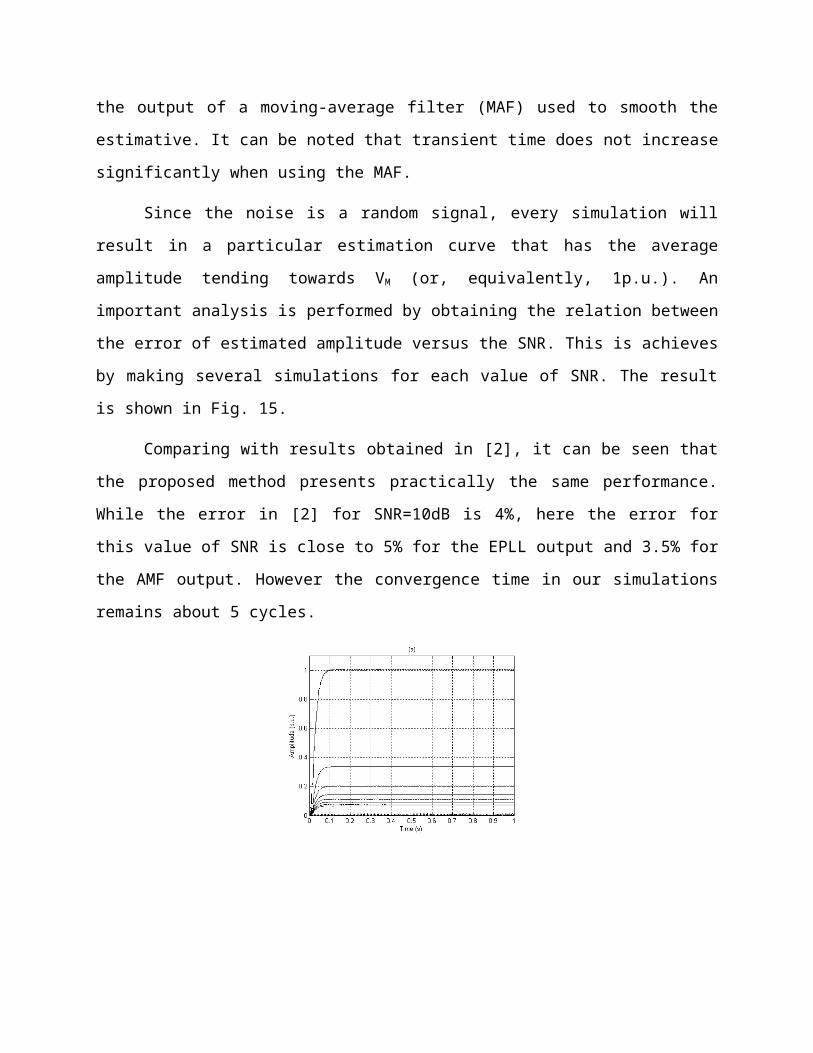
Being the inverter operated by a PWM technique, the rectifier is an uncontrolled diode

bridge, as reported in the typical scheme shown in Fig. 2.

Fig. 2. PWM drive scheme.

A. DC-Link

The harmonics produced by the rectifier, those produced by the inverter and the

interharmonics due to the interaction between the two converters are present in both DC-link

currents, idcr(t) and idci(t). The harmonic frequencies generated by the rectifier can be calculated

using formula (1) because the rectifier operation does not change.

The harmonic frequencies generated by the inverter (see Appendix B) are evaluated as:

(8)

with j and r integers depending on the modulation ratio as reported in Table I; the dependency

from mf is related to the switching strategy adopted as shown in the following Section VI. In

particular, Table I shows that:

both even and odd harmonics are present for even mf;

only even harmonics are present for odd mf;

only triple harmonics are present for triple mf.

Table I: Values of parameters j and r for different mf choices

mf Odd even

non triple j r j r

Even

integers

even

integers

even

integers

integers

Odd

integers

odd

integers

odd

integers

triplej r j r

even

integers

even triple

integer

even

integers

triple

integers

odd

integers

odd triple

integer

odd

integers

The interharmonics due to the intermodulation operated by the two converters are also

present [9]. Their frequencies are evaluated according to the following relationship:

(9)

with =1,2,3,…, j and r as in Table I.

B. Supply System Side

For the harmonic frequencies of iss(t) the same considerations developed in Section III

apply and formula (4) is still valid.

The interharmonic frequencies of iss(t) derive from the modulation of the inverter

harmonic components (8) operated by the rectifier and can be evaluated according to the

following relationship:

(10)

with =1,2,3,… j and r as in Table I.

As for the sequences, the same considerations about (4) and (5) still apply.

C. Output Side

The harmonic frequencies of ios(t) are evaluated as shown in Appendix B; it is:

(11)

with j and k as in Tab. II.

Table II: Values of parameters j and k for different mf choices

mf odd Even

J k j k

even

integers

odd

integers

even

integers

integers

odd integers even

integers

odd

integers

The interharmonic frequencies of ios(t) derive from the modulation of the rectifier

harmonic components (1) operated by the inverter and can be evaluated according to the

following relationship:

(12)

with j and k as in Table II, =1,2,3,….

Also in this case, the sequences of the harmonics in (11) determine the sequences of the

interharmonics in (12) according to the same rules shown in Section III.

10.6 Symbolism Proposal

In order to find out the origins of a given interharmonic component produced by the

interaction between rectifier and inverter inside the ASD and under ideal supply conditions, it

seems useful to introduce a proper symbolism. Reference is made to the interharmonic

components in both the supply system and output sides. Though harmonic order calculation is

different in LCI and PWM drives it is, anyway, possible to find a unified and, at the same time,

easy to understand symbolism.

Concerning the supply system side interharmonics, it seems suitable to introduce the

symbols:

, (13)

, (14)

where:

- the subscripts evidence the common origin of the couple of components (13) and (14)

related to the rectifier harmonic of order hss (see (4)) and to the inverter DC-link harmonic of

order hosdc (see (2) for LCI and (8) for PWM) involved in the intermodulation process;

- the superscript distinguishes the relative position of the components, being “u” for the

component (13), which stands “up” in frequency due to sign “+” in (5), for LCI, and (10), for

PWM, and “d” for the other component (14), which stands “down” in frequency due to the

sign “-” in (5), for LCI, and (10), for PWM.

An example of the application of the aforementioned symbols is reported in the

following Section (Fig. 4 for LCI and Fig. 8 for PWM ).

Concerning the output side interharmonics, it seems suitable to introduce the symbols:

, (15)

, (16)

where:

- the subscripts evidence again the common origin of the couple of components (15) and (16)

related to the inverter harmonic of order hos (see (6) for LCI and (11) for PWM) and to the

rectifier DC-link harmonic of order hssdc (see (1) for both LCI and PWM) involved in the

intermodulation process;

- the use of the superscript is the same as for the supply side components (15) and (16) but,

this time, it is related to the signs (“+” and “-“) in (7), for LCI, and (12), for PWM.

An example of the application of the aforementioned symbols is reported in the

following Section (Fig. 5 for LCI and Fig. 9 for PWM).

10.7 Numerical Analyses

Several numerical analyses were carried out on both LCI and PWM typical drives, both

characterized by qss and qos equal to six; their other parameters are fully referenced in [8] and

[9] respectively. The models proposed in [8] and [9], validated comparing their results with

those obtained by means of the well known software EMTP and Power System Blockset under

Matlab environment, were used.

Some experimental verifications of the formulas developed in the chapter are reported

in [3] and [13] for LCI drives and in [14] and [15] for PWM drives. In all the cases the frequency

components expected according to the formulas (4)-(7) and to (10)-(12) respectively, were

always actually present and of prevalent amplitude. Some additional frequency components

were measured and it was demonstrated that their origin was the interaction between the non

ideal supply system and ASDs, not covered by the formulas of Section III and IV.

A. LCI Drive

Figure 3 shows the LCI drive interharmonic frequency values versus output frequency

values, for both the supply system and output sides, obtained using (5) and (7). For the sake of

clarity, only some specified interharmonic components are reported.

Figures 4a) and 5a) show the amplitudes of current interharmonics versus their

frequencies for fos=40Hz, and refer to the supply system and output sides, respectively. Figures

4b) and 5b) show how to use the plots of Figs. 3a) and 3b), respectively, to forecast the

interharmonic component frequencies. The couple of the main interharmonics in Fig. 4a), Iu1,6

and Id1,6, is generated by the intermodulation between the 1st supply system harmonic and the

6th DC-link harmonic produced by the inverter. The main interharmonic in Fig. 5a) is Id11,6, while

Id7,6, of smaller but still remarkable amplitude, seems particularly notable due to its low

frequency (20 Hz), which can create problems to asynchronous motor life [17].

Fig. 3. LCI drive interharmonic frequencies versus output frequency:

a) supply system side, all interharmonics due to (j) of (5) = (1,1), (1,2), (1,3), (2,1), (2,2), (2,3), (3,1), (3,2), (3,3), (4,1), (4,2), (4,3);

b) output side, all interharmonics due to (j,) of (7) = (1,1), (1,2), (1,3), (2,1), (2,2), (2,3), (3,1), (3,2), (3,3), (4,1), (4,2), (4,3).

Fig. 4. LCI drive supply system current interharmonics for fos= 40Hz:a) amplitudes in percentage of 230A versus interharmonic frequency;

b) frequencies (abscissa) versus output frequency (ordinate).

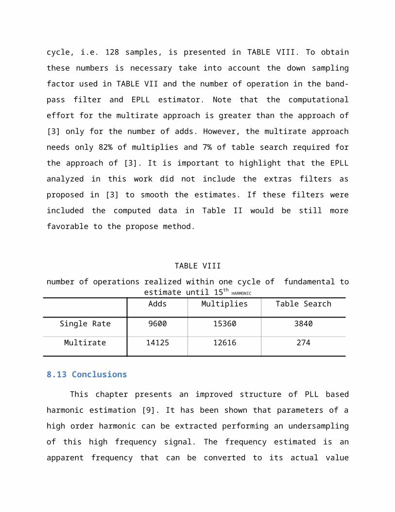
Fig. 5. LCI drive output current interharmonic for fos= 40Hz:a) amplitudes in percentage of 165A versus interharmonic frequency;

b) frequencies (abscissa) versus output frequency (ordinate).

B. PWM drive

The inverter modulation strategy selected is represented in Fig. 6 in terms of actual, fsw,

and mean, f*sw, switching frequency (see Appendix B); a constant value of f*

sw for all the output

frequencies is assumed equal to 350 Hz. Fig. 6 reports also the modulation ratio, m f. It is

possible to observe that the modulation ratio varies during the ASD operation so changing the

order of the harmonic components injected both into the DC-link and into the output side.

The plots in Fig. 7, obtained by means of (10) and (12), show the interharmonic

frequency values versus the output frequency both in the supply system and output sides,

according to the switching frequency trend of Fig. 6. Only some specified interharmonic

components are reported to make it easier to understand the plots: f.i. in Fig.7a) the

interharmonic components due to the intermodulation of the first harmonic of the rectifier

(=1) with the harmonic components generated by different couples of j and r, that is to say the

intermodulation produced by specified side bands of the DC spectrum produced by the inverter

are represented.

Concerning the supply system side, it is evident that the overlapping of different

interharmonic components occurs for some output frequency ranges. The most remarkable

overlappings are highlighted by the grey shadows in Fig. 7a). Of course, such overlapping leads

to synergic combinations of interharmonic components originated from different

intermodulations. As for the output side, the aforementioned overlapping occurs only for

discrete frequency values.

Figures 8a) and 9a) show the amplitudes of the current interharmonics versus their

frequencies for fos=40 Hz and mf=9, with reference to the supply system and output sides,

respectively.

Figures 8b) and 9b) show how to use the plots of Figs. 7a) and 7b) to forecast the

interharmonic component frequencies. It is worthwhile noting that overlapping causes that the

interharmonic components due to the values of the parameters (,mf,j,r) in (10) equal to

(1,9,0,6) and to (1,9,1,3) have the same frequencies producing Iu1,6 and Id

1,6 (see Fig. 8a)).

In Fig. 10 the behaviours of the two supply side interharmonic components due to

(1,mf,0,6) and (1,mf,1,3) in (10) in terms of amplitude (Fig. 10a) and Fig. 10b)) and frequency

(Fig. 10c)) variations versus the output frequency are shown. The overlapping occurs in the

output frequency range (see Fig. 10c) in the interval 3741 Hz where mf=9). Finally, it can be

observed that the interharmonic due to (1,mf,1,3) of (10) degenerates in the 5-th harmonic

twice (fos= 15 Hz and fos=20 Hz).

Fig. 6. PWM drive: switching frequency (fsw) and modulation ratio (mf.)

Fig. 7. PWM drive interharmonic frequencies versus output frequency:a) supply system side: all interharmonics due to =1, mf as in Fig. 6 and

(j,r) of (10) = (0,6), (1,3), (1,9), (2,0), (2,6), (3,3), (3,9), (4,0), (4,6);b) output side: all interharmonics due to mf as in Fig. 6,=1 and

(j,k) of (12) = (0,1), (0,3), (1,0), (1,2), (2,1), (2,3), (3,0), (3,2), (4,1), (4,3).

Fig. 8. PWM drive supply system current interharmonics: a) amplitudes in percentage of 248A versus interharmonic frequency; b) frequencies (abscissa) versus output frequency (ordinate)

with switching frequency of Fig. 6.

Fig. 9. PWM drive output current interharmonics: a) amplitudes in percentage of 423A versus interharmonic frequency; b) frequencies (abscissa) versus output frequency (ordinate) with switching frequency of Fig. 6.

Fig. 10. PWM drive supply system interharmonics versus output frequency, with switching frequency of Fig. 6: amplitude of the component generated by the values of the parameters (,mf,j,r) in (10) equal to a) (1,mf,1,3) and b) (1,mf,0,6); c) corresponding interharmonic frequency versus output frequency.

10.9 Conclusions

The interharmonic generation process has been addressed with reference to high power

Adjustable Speed Drives based on double stage conversion systems using Line Commutated or

Pulse Width Modulated Inverters. Reference has been made to ideal supply conditions.

Formulas to forecast the interharmonic frequencies due to the interaction between the rectifier

and inverter have been developed and a proper symbolism has been proposed to recognize the

interharmonic origins. Numerical analyses have been performed for both the considered ASDs

in a wide range of output frequencies, giving a comprehensive insight in the complex behaviour

of interharmonic component frequencies. Some characteristic aspects, such as the

degeneration of interharmonic components in harmonics or the overlapping of a couple of

interharmonics of different origins, have been highlighted.

Appendix A

Reference is made to a q-pulse bridge converter operating synchronously with the AC

side; the current on the DC side is affected by a ripple superimposed on the direct component,

IDC. The results apply to both rectifier and inverter operation and, for this reason, the subscripts

“ss” and “os” are omitted.

As it is well known, the bridge can be seen (Fig. A1) as having two inputs: the “switching

function”, Sw(t), and the “modulating function”, that is the current on the DC side, idc(t).

In other words, the bridge acts as a modulator and its output, the current on the AC

side, iac (t), is said to be “modulated”.

Fig. A1. q-pulse bridge converter.

The switching function Sw(t) can be expressed using the Fourier series:

(A1)

where (12)

is the peak magnitude of sinusoidal components and () its phase-angle, ac is the fundamental

angular frequency of the AC side, and q is the number of pulses of the bridge converter.

The “modulating” function idc (t) can be expressed in a general form as the sum of the direct

current and of superimposed sine waves:

(A2)

where is the peak magnitude of sinusoidal components on the DC side and () its phase-

angle; dc can assume any value and it is not necessarily an integer multiple of ac.

The “output” of the bridge, iac(t), can be found by multiplying the switching function

Sw(t) by the “modulating” function idc(t):

(A3)

that by applying the Werner formula can be written as:

(A4)

The last two series of the formula above show that, under the considered conditions,

the three phase bridge converters generate interharmonics, which are passed into the AC side,

and which are in addition to the normal theoretical harmonics of ac (of 1st, 5th, 7th, 11th, 13th,

etc, orders).

Appendix B

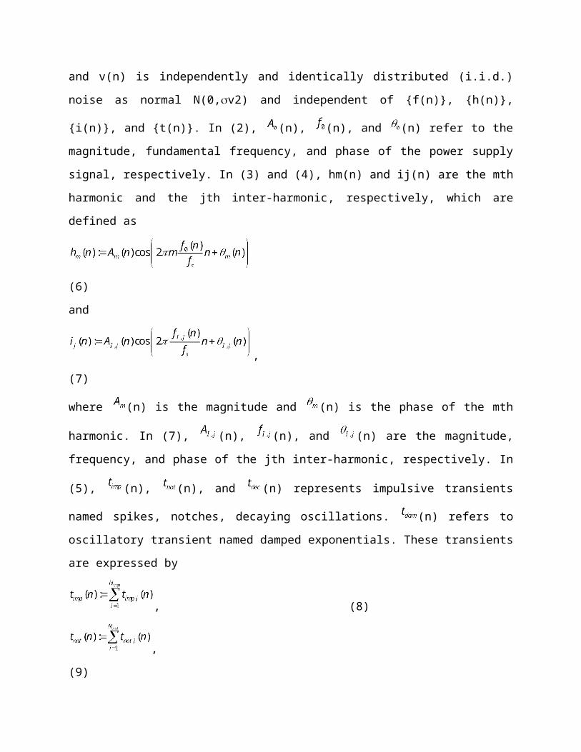
Reference is made to the circuit of Fig. B1 in which, for the sake of simplicity, a constant

DC voltage, Vdc, is considered.

Fig. B1. PWM inverter supplying steady-state motor model.

Figure B2 shows the sinusoidal PWM: if synchronous PWM is adopted, mf must be an

integer number.

The voltage vAO(t), defined with reference to Fig. B1, is obtained by comparing the

carrier signal, (t), with the modulation signal, cAO(t) (see Fig. B2). Similarly, vBO(t) and vCO(t) are

obtained by comparing (t) with two modulation signals, cBO(t) and cCO(t), with a phase shifting

from cAO(t) of –120° and +120°, respectively.

Fig. B2. Sinusoidal PWM: a) cAO(t) is the sinusoidal modulation signal for the phase A, (t) is the carrier signal; b) vAO(t) is the voltage defined with reference to Fig. B1.

Referring to the symbolism of Fig. B1 and supposing that the inverter does not dissipate

or generate power and that the load is balanced, it results:

(B1)

The harmonic components of idci(t) are obtained by modulating harmonics of vAO(t), vBO(t)

and vCO(t) with those of iAos(t), iB

os(t) and iCos(t), respectively. It is worthwhile noting that

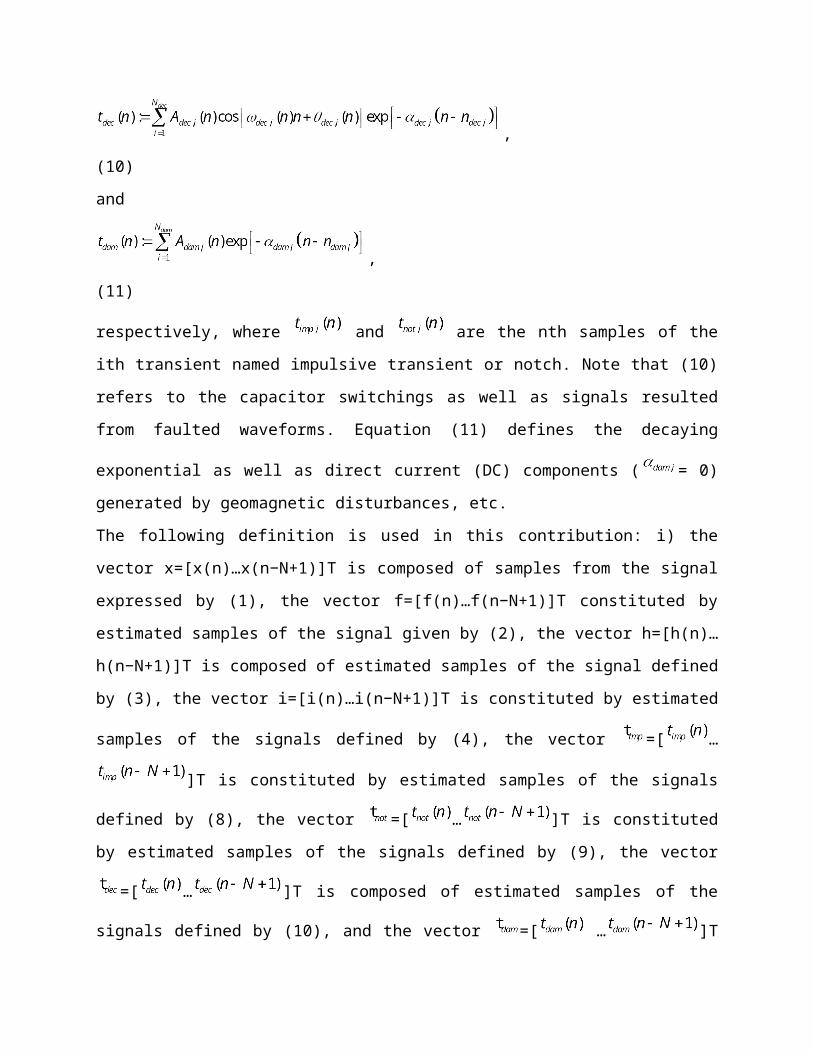
vXO(t)/Vdc, with X= A, B, C, represents the well-known inverter switching function.

If mf is an integer, vAO(t), vBO(t) and vCO(t) have fos as fundamental frequency and only

harmonic components are present. Moreover, if mf is an odd integer, vAO(t), vBO(t) and vCO(t)

contain only odd harmonics and their DC components, V0, are exactly Vdc/2; instead, if mf is an

even integer, they contain both odd and even harmonics and the DC components may be

different from Vdc/2.

A general expression can be written:

(B2)

where X= A, B, C and

(B3)

The amplitudes An are calculated as:

(B4)

where X is the phase of cXO(t) and:

(B5)

Some simplifications can be obtained if mf is odd; assuming that:

(B6)

formulas (B3), (B4) and (B5) can be rewritten as:

(B7)

with

(B8)

However, if mf is even, j and k can assume all integer values.

So, the harmonic frequency components of vXO(t) can be evaluated according to the

following relationship:

(B9)

where j and k vary as shown in Tab. II in section IV.

Due to the inverter load model adopted, harmonic components of iXos(t) are located at

the same frequencies as those of the corresponding voltages.

The harmonic frequencies of idci(t) can be deduced by means of the modulation theory: the

harmonic components of iXos(t) are modulated according to (B1) and its harmonic frequencies

are evaluated according to:

(B11)

So, formula (8) is obtained by (B11), writing (k1) as r.

Finally, it is worthwhile observing that the modulation strategy depends on the relation

between the actual switching frequency, fsw, and fos according to:

(B12)

being mf(fos), in general, a proper function representing the modulation ratio, and assuming

integer values for synchronous PWM:

(B13)

being round(.) the function which gives the integer nearest to the argument and f*sw the

asynchronous switching frequency which depends on the control strategy [18].

References

[1] Yacamini, R., Power system harmonics. IV. Interharmonics, Power Engineering Journal,

Volume: 10, Issue: 4 , Aug. 1996.

[2] IEEE Interharmonic Task Force, "Interharmonic in Power System," Cirgré 36.05/CIRED 2

CC02 Voltage Quality Working Group,

http://grouper.ieee.org/groups/harmonic/iharm/docs/ihfinal.pdf.

[3] R. Carbone, D. Menniti, R. E. Morrison, E. Delaney, and A. Testa, "Harmonic and

Intherarmonic Distortion in Current Source Type Inverter Drives," IEEE Trans. on Power

Delivery, Vol. l0, n. 3, pp. 1576-1583, July 1995.

[4] M. B. Rifai, T. H. Ortmeryer, W. J. McQuillan, "Evaluation of Current Interharmonics from AC

Drives," IEEE Trans. on Power Delivery, Vol.15, No.3, July 2000, pp.1094-1098.

[5] R. Carbone, D. Menniti, R. E. Morrison, and A. Testa, "Harmonic and Intherarmonic

Distortion Modelling in Multiconverter System," IEEE Trans. on Power Delivery, Vol. l0, n. 3,

pp. 1685-1692, July 1995.

[6] R. Carbone, A. Lo Schiavo, P. Marino, and A. Testa, "Frequency coupling matrixes for multi

stage conversion system analysis," European Transactions on Electric Power Systems Vol.

12, No. 1, January/February 2002..

[7] W. Xu, H. W. Dommel, M. Brent Hughes, G. W. K. Chang, L. Tan, "Modelling of Adjustable

Speed Drives for Power System Harmonic Analysis," IEEE Trans. on Power Delivery, Vol.14,

No.2, April 1999, pp.595-601.

[8] R. Carbone, F. De Rosa, R. Langella, and A. Testa, "A New Approach to Model AC/DC/AC

Conversion Systems," IEEE/PES Summer Meeting, July 2001, Vancouver, CANADA.

[9] R. Carbone, F. De Rosa, R. Langella, A. Sollazzo, and A. Testa, "Modelling of AC/DC/AC

Conversion Systems with PWM Inverter," IEEE/PES Summer Meeting, July 2002, Chicago,

U.S.A..

[10] M. Sakui and H. Fujita, "Calculation of harmonic currents in a three-phase converter with

unbalanced power supply conditions," IEE Proc.B, Vol. 139, No.5, September 1992, pp. 478-

484.

[11] L. Hu and R. Morrison, "The Use of the Modulation Theory to Calculate the Harmonic

Distortion in HVDC Systems Operating on an Unbalanced Supply," IEEE Trans. on Power

Systems, Vol. 12, No. 2, May 1997, pp.973-980.

[12] D. Castaldo, F. De Rosa, R. Langella, A. Sollazzo, A. Testa, “Waveform Distortion Caused by

High Power Adjustable Speed Drives Part II: Probabilistic Analysis,” ETEP, Vol. 13, No. 6,

November/December 2003, pages 355-363.

[13] R. Carbone, V. Mangoni, C. Mirone, P. Paternò, and A. Testa, "Interharmonic distortion in

the static strarting-up system of a hydro-electric pumped-storage power station," 7-th IEEE

ICHQP Las Vegas, NV, U.S.A. October 16-18, 1996.

[14] P.Caramia, G.Carpinelli, P.Varilone, D.Gallo, R.Langella, A.Testa P. Verde, “High Speed Ac

Locomotives: Harmonic And Interharmonic Analysis At A Vehicle Test Room”, invited paper

at 9th IEEE International Conference on Harmonics and Quality of Power, Orlando, USA, 1-4

October 2000.

[15] R. Carbone, F. De Rosa, R. Langella, A. Sollazzo, A. Testa, "Modeling Waveform Distortion

Produced by High Speed AC Locomotive Converters," IEEE PowerTech2003, June 2003,

Bologna, Italy.

[16] A.V.Oppenheim, R.W.Schaffer, Discret time signal processing, Prentice-Hall International

Inc., 1989.

[17] J. Policarpo G. de Abreu and A. E. Emanuel, "Induction motors loss of life due to voltage

imbalance and harmonic: a preliminary study," 9th ICHQP, Orlando, Florida, U.S.A. October

1-4, 2000.

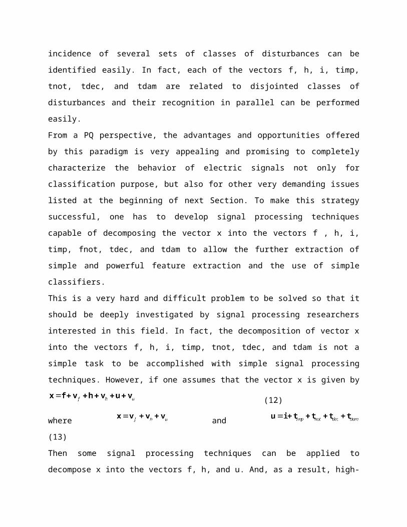
[18] J.M.D. Murphy and F.G. Turnbull, Power electronic control of AC motors, Pergamon press.

11.1 Introduction

Although it is well known that Fourier analysis is in reality only accurately applicable to

steady state waveforms, it is a widely used tool to study and monitor time-varying signals,

which are commonplace in electrical power systems. The disadvantages of Fourier analysis,

such as frequency spillover or problems due to sampling (data window) truncation can often be

minimized by various windowing techniques, but they nevertheless exist. This chapter

demonstrates that it is possible to track and visualize amplitude and time-varying power

systems harmonics, without frequency spillover caused by time-frequency techniques. This new

tool allows for a clear visualization of time-varying harmonics which can lead to better ways to

track harmonic distortion and understand time-dependent power quality parameters. It also

has the potential to assist with control and protection applications. While estimation technique

is concerned with the process used to extract useful information from the signal, such as

amplitude, phase and frequency; signal decomposition is concerned with the way that the

original signal can be split in other components, such as harmonic, inter-harmonics, sub-

harmonics, etc..

Harmonic decomposition of a power system signal (voltage or current) is an

important issue in power quality analysis. There are at least two reasons to focus on harmonic

decomposition instead of harmonic estimation: (a) if separation of the individual harmonic

component from the input signal can be achieved, the estimation problem becomes easier; (b)

Chapter 11 - Novel Method for Tracking Time-Varying Power Harmonic Distortions without

Frequency Spillover

C. A. Duque, P.M. Silveira, T. Baldwin, P. F. Ribeiro

the decomposition is carried out in the time-domain, such that the time-varying behavior of

each harmonic component can be observed.

Some existing techniques can be used to separate frequency components. For example,

STFT (Short Time Fourier Transform) and Wavelets Transforms [1], are two well known

decomposition techniques. Both can be seen as a particular case of filter bank theory [2]. The

STFT coefficients filters are complex numbers which generates a complex output signal whose

magnitude corresponds to the amplitude of the harmonic component being estimated [2]. The

main disadvantage of this method is to set up an efficient band-pass filter with lower frequency

spillover. On the other hand, although wavelet transform utilizes filters with real coefficients,

the common wavelet mothers do not have good magnitude response in order to prevent

frequency spillover. Besides, the traditional binary tree structure is not able to divide the

spectrum conveniently for harmonic decomposition.

Adaptive notch filter and PLL (Phase-Locked Loop) [3]-[4] have been used for extracting

time-varying harmonics components. However, these methods work well only if a few

harmonics components are present at the input signal. In the other case the energy of adjacent

harmonics spills over each other and the decomposed signal becomes contaminated. In [5] the

authors presented a technique based on multistage implementation of narrow low-pass digital

filters to extract stationary harmonic components. Thus, no digital analytical technique has

been proposed or used to track time-varying power systems harmonics without frequency

spillover. Consequently, the method proposed in this chapter adequately utilizes filters banks to

avoid the frequency mixture, particularly associated with time-varying signals.

Attempts to visualize time-varying harmonics using Wavelet Transform have been

proposed in [6] and [7]. However, the structures were not able to decouple the frequencies

completely.

The methodology proposed in this chapter is constructed to separate the odd and the

even harmonic components, until the 15th. It uses selected digital filters and down-sampling to

obtain the equivalent band-pass filters centered at each harmonic. After the signal is

decomposed by the analysis bank, each harmonic is reconstructed using a non-conventional

synthesis bank structure. This structure is composed of filters and up-sampling that

reconstructs each harmonic to its original sampling rate.

The immediate use for this method is the monitoring of time-varying individual power

systems harmonics. Future use may include control and protection applications, as well as inter-

harmonic measurements.

The chapter is divided into method description, odd/even harmonic extraction and

simulation results.

11.2 Method descriptionMultirate systems employ a bank of filters with either a common input or summed

output. The first structure is known as analysis filter bank [8] as it divides the input signal in

different sub-bands in order to facilitate the analysis or the processing of the signal. The second

structure is known as synthesis filter bank and is used if the signal needs to be reconstructed.

Together with the filters the multirate systems must include the sampling rate alteration

operator (up and down-sampling). Figure 1 shows two basic structures used in a multirate

system, where the up and down-sampling factor, M and L, equal 2. Figure 1-a shows a

decimator structure composed by a filter following by the down sampler and Fig. 1-b the

interpolator structure composed by a up-sampler followed by a filter. The decimator structure

is responsible to reduce the sampling rate while the interpolator structure to increase it. The

filters H(z) and F(z) are typically band-pass filters.

Fig. 1- Basic structures used in multirate filter bank and its equivalent representation for

L=M=2. (a) Decimator; (b) Interpolator

The direct way to build an analysis filter bank, in order to divide the input signal in its

odd harmonic component, is represented in Fig. 2. In this structure the filter is a band-

pass filter centered in the kth harmonic and must be projected to have 3dB bandwidth lower

than 2f0 , where f0 is the fundamental frequency. If only odd harmonics are supposed to be

present in the input signal, the 3dB bandwidth can be relaxed to be lower than 5f0. Note that

Fig. 2 is not a multirate system, because the structure does not include sampling rate

alternation, which means that there is only one sampling rate in the whole system.

The practical problem concerning the structure shown in Fig. 2 is the difficulty to design

each individual band-pass filter. This problem becomes more challenging when a high sampling

rate must be used to handle the signal and the consequent abrupt transition band.

In this situation the best way to construct an equivalent filter bank is to utilize the

multirate technique. Figure 3 shows how an equivalent structure to Fig.2 can be obtained using

the multirate approach. The filters H0(z) and H1(z) are orthogonal filters [6], with the first one

as a low-pass filter and the second one as a high-pass filter.

Fig. 2 – Analysis bank filter to decomposed the input signal in its harmonics components.

.

Fig.3- Multirate equivalent structure to the filter bank in Fig.2

Figure 4 shows the amplitude response for the analysis bank. This figure was obtained

using sampling rate equal to 256 samples by cycle and FIR filters of 69th order. These filters

correspond to so-called orthogonal filter banks also known as power-symmetric filter banks [8].

0 2 4 6 8 10 12 14 16 18-40

-35

-30

-25

-20

-15

-10

-5

0

frequency (harmonic number)

Mag

nitu

de (d

B)

Analysis Filter Bank Frequency Response

H1 H3 H5 H7 H9 H11 H13 H15

Fig. 4- Amplitude response in dB (frequency axis is labeled with the harmonic number)

The main difference between the structure shown in Fig. 2, and the other one obtained

using the multirate technique, is the decimator at the output of the bank, as shown in Fig. 5. In

fact, Fig.5 is equivalent to Fig. 3. It was obtained using the multirate nobles identities [2] and

moving the downsampler factor inside Fig.2 to the right side. The decimated signal at the

output of each filter has a sampling rate 64 times lower then the input signal. To reconstruct

each harmonic into its original sampling rate it is necessary to use the synthesis filter bank

structure.

Fig. 5- Equivalent multirate analysis filter bank

11.3 The synthesis filter banksThe synthesis filter bank used here is a different implementation of the conventional

one. As the interest is to reconstruct each harmonic instead of the original signal, the filter bank

must be divided in order to obtain the corresponding harmonic. Figure 6 shows the filter bank

utilized to reconstruct the harmonic components.

Fig. 6- Modified synthesis bank

It is important to remark that the frequency response of the synthesis filter bank is

similar to Fig. 4.

The analysis of Fig. 4 reveals that the filter bank in this configuration is unable to filter

even harmonics appropriately, what means that these components will appear with the

adjacent odd harmonics. To overcome this problem an additional filter stage is included. This

filter is composed by a second order Infinite Impulse Response (IIR) notch filter.

11.4 Extracting even harmonicsTo extract the even harmonics the same bank can be used together with a

preprocessing of the input signal. Hilbert transform is then used to implement a technique

known as Single Side Band (SSB) modulation [8]. The SSB modulation moves to the right all

frequencies in the input signal by f0 Hz. In this way, even harmonics are changed to odd

harmonics and vice-versa.

Figure 7 shows the whole system for extracting odd and even harmonics.

Fig. 7 – Whole structure to harmonic extraction

11.5 Simulation resultsThis section presents two examples: the first is a synthetic signal, which has been

generated in Matlab using a mathematical model, and the second is a signal obtained from the

Electromagnetic Transient Program including DC systems (EMTDC) with its graphical interface

Power Systems Computer Aided Design (PSCAD). This program can simulate any kind of

power system with high fidelity and the resulting signals of interest are very close to physical

reality.

Synthetic Signal

The synthetic signal utilized can be represented by:

(1)

Where h is the order (1 up to 15th) and A is the magnitude of the component, 0 is the

fundamental frequency, and finally, f(t) and g(t) are exponential functions (crescent, de-

crescent or alternated one) or simply a constant value . Besides, x(t) is partitioned in four

different segments in such way that the generated signal is a distorted one with some

harmonics in steady-state and others varying in time, including abrupt and modulated change

of magnitude and phase, as well as a DC component. Figure 8 illustrates the synthetic signal.

The structure shown in Fig. 7 has been used to decompose the signal into sixteen

different harmonic orders, including the fundamental (60 Hz) and the DC component.

Figure 9 shows the decomposed signal which its corresponding components from DC up

to 11th harmonic. The left column represents the original components and the right column the

corresponding components obtained through the filter bank.

For simplicity and space limitation the higher components are not shown. However, it is

important to remark that all waveforms of the time-varying harmonics are extracted with

efficiency along the time.

Naturally, intrinsic delays will be present during the transitions from previous to the new

state. Figure 10 shows some components of both the original and decomposed signal in a short

time scale interval.

0 0.5 1 1.5 2 2.5 3 3.5 4-3

-2

-1

0

1

2

3

4

5

Mag

nitu

deTime (s)

Fig. 8 – Synthetic signal used

Simulated Signal

It is well known that during energization a transformer can draw a large current

from the supply system, normally called inrush current, whose harmonic content is high.

Although today’s power transformers have lower harmonic content Table 1, shows the

typical harmonic components present in the inrush currents [9]. These values are normally used

as reference for protection reasons, but they do not take into account the time-varying nature

of this phenomenon.

Table 1- typical harmonic content of the inrush current

Order Content %

Dc 55

2 63

3 26.8

4 5.1

5 4.1

6 3.7

7 2.4

In recent years, improvements in materials and transformer design have lead to inrush

currents with lower distortion content [10]. The magnitude of the second harmonic, for

example, has dropped to approximately 7% depending on the design [11]. But, independent of

these new improvements, it is always important to emphasize the time-varying nature of the

inrush currents.

In being so, a transformer energization case was simulated using EMTDC/PSCAD and the

result is shown in Fig. 11.

Using the methodology proposed to visualize the harmonic content of the inrush

current, Fig. 12 reveals the rarely seen time-varying behavior of the waveform of each harmonic

component, where the left column shows the DC and even components and the right column

the odd ones. This could be used to understand other physical aspects not observed previously.

0 1 2 3 40

1

2DC component

0 1 2 3 40

1

2DC component

0 1 2 3 4-1

0

11st

0 1 2 3 4-1

0

11st

0 1 2 3 4-1

0

12nd

0 1 2 3 4-1

0

12nd

0 1 2 3 4-1

0

13rd

Time s0 1 2 3 4

-1

0

13rd

Time s

0 1 2 3 4-1

0

14th

0 1 2 3 4-1

0

14th

0 1 2 3 4-0.5

0

0.55th

0 1 2 3 4-0.5

0

0.55th

0 1 2 3 4-0.2

00.2

6th

0 1 2 3 4-0.2

00.2

6th

0 1 2 3 4-0.5

0

0.57th

Time s0 1 2 3 4

-0.5

0

0.57th

Time s

0 1 2 3 4-1

0

18th

0 1 2 3 4-1

0

18th

0 1 2 3 4-0.2

00.2

9st

0 1 2 3 4-0.2

00.2

9st

0 1 2 3 4-1

0

110th

0 1 2 3 4-1

0

110th

0 1 2 3 4-0.5

0

0.511rd

Time s0 1 2 3 4

-0.5

0

0.511rd

Time s

Fig. 9 – First column: original components, second column: decomposed signals.

2.99 3 3.01 3.02 3.03 3.04 3.050

1

2DC component

2.99 3 3.01 3.02 3.03 3.04 3.05-1

0

12nd

2.99 3 3.01 3.02 3.03 3.04 3.05-1

0

13rd

2.99 3 3.01 3.02 3.03 3.04 3.05-0.5

0

0.57th

Time s

Fig. 10 – Comparing original and decomposed component

0 0.1 0.2 0.3 0.4 0.5 0.6 0.7 0.8 0.9 1-2

0

2

4

6

8

10

12

14

Time (s)

Mag

nitu

de k

A

Fig. 11 – Inrush current in phase A.

Table 1- typical harmonic content of the inrush current

Order Content %

Dc 55

2 63

3 26.8

4 5.1

5 4.1

6 3.7

7 2.4

11.6 Final consideration and future work The methodology proposed has some intrinsic limitations associated with the

analysis of inter-harmonics as well as with real time applications. The Inter-harmonics (if they

exist) are not filtered by the bank, so it would corrupt the nearby harmonic components. The

limitation regarding with real time applications is related to the transient time response

produced by the filter bank. For example, in the presence of abrupt change in the input signal,

such as in inrush currents, the transient response can last more than 5 cycles, which is not

appropriate for applications whose time delay must be as short as possible. The computational

effort for real time implementation is another challenge that the authors are investigating. In

fact the high order filter (69th) used in the bank structure demand high computational effort.

By using multirate techniques to implement the structure it is possible to show that the number

of multiplication by second to implement one branch of the analysis filter bank is about one

million. Some low price DSPr (Digital Signal Processors) available in the market are able to

execute 300 Million Float Point operations per second. This shows that, despite the higher

computational effort of the structure, it is feasible to be implemented in hardware. However,

new opportunities exist for overcoming the limitations and the development of improved and

alternative algorithms. For example, the authors are investigating the possibility of extracting

inter-harmonic components and developing a similar methodology based on Discrete Fourier

Transform (DFT). The first results show similar visualization capabilities with the promise to

provide a reduced transient time response and lower computational burden. This process has

the potential of addressing specific protective relaying needs such as detecting a high

impedance fault during transformer energization and detection of ferro-resonance.

0 0.2 0.4 0.6 0.8 10

2

4DC component

0 0.2 0.4 0.6 0.8 1-5

0

51st

0 0.2 0.4 0.6 0.8 1-202

2nd

0 0.2 0.4 0.6 0.8 1-1

0

13rd

Time sTime s

0 0.2 0.4 0.6 0.8 1-0.5

0

0.54th

0 0.2 0.4 0.6 0.8 1

-0.20

0.2

5th

0 0.2 0.4 0.6 0.8 1-0.2

0

0.26th

Time (s)0 0.5 1

-0.10

0.1

7th

0 0.2 0.4 0.6 0.8 1

-0.1

0

0.1

8th

0 0.2 0.4 0.6 0.8 1-0.1

0

0.19st

0 0.2 0.4 0.6 0.8 1

-0.050

0.05

10th

0 0.2 0.4 0.6 0.8 1

-0.05

0

0.05

11rd

0 0.2 0.4 0.6 0.8 1-0.05

0

0.0512th

0 0.2 0.4 0.6 0.8 1-0.05

0

0.0513th

0 0.2 0.4 0.6 0.8 1-0.04-0.02

00.020.04

14th

Time (s)0 0.2 0.4 0.6 0.8 1

-0.05

0

0.0515th

Time (s)

Fig. 12 – Decomposition of the simulated transformer inrush current.

11.7 Conclusions

This chapter presents a new method for time-varying harmonic decomposition based on

multirate filter banks theory. The technique is able to extract each harmonic in the time

domain. The composed structure was developed to work with 256 samples per cycle and to

track up to the 15th harmonic. The methodology can be adapted through convenient pre-

processing for different sampling rates and higher harmonic orders.

Acknowledgments

The authors would like to thanks Dr. Roger Bergeron and Dr. Mathieu van den Berh for

their useful and constructive suggestions.

11.8 References

[1] Yuhua Gu, M. H. J. Bollen, “Time-Frequency and Time-Scale Domain Analysis,” IEEE

Transaction on Power Delivery, Vol. 15, No. 4, October 2000, pp. 1279-1284.

[2] P.P. Vaidyanathan, Multirate Systems and Filter Banks, Prentice Hall, 1993.

[3] M. Karimi-Ghartemani, M. Mojiri and A. R. Bakhsahai, “A Technique for Extracting

Time-Varying Harmonic based on an Adaptive Notch Filter,” Proc. of IEEE Conference on Control

Applications, Toronto, Canada, August 2005.

[4] J. R. Carvalho, P. H. Gomes, C. A. Duque, M. V. Ribeiro, A. S. Cerqueira, and J.

Szczupak, “PLL based harmonic estimation,” IEEE PES conference, Tampa, Florida-USA, 2007

[5] C.-L. Lu, “Application of DFT filter bank to power frequency harmonic measurement,”

IEE Proc. Gener. , Transm,. Distrib., Vol 152, No.1, January 2005, pp. 132-136.

[6] P. M. Silveira, M. Steurer, .P F. Ribeiro, “Using Wavelet decomposition for

Visualization and Understanding of Time-Varying Waveform Distortion in Power System,” VII

CBQEE, August 2007, Brazil.

[7] V.L. Pham and K. P. Wong, “Antidistortion method for wavelet transform filter banks

and nonstationay power system waveform harmonic analysis,” IEE Proc. Gener., Transm.,

Distrib., Vol 148, No.2, March 2001, pp. 117-122.

[8] Sanjit K. Mitra, Digital Signal Processing – A computer-based approach, Mc-Graw Hill

2006, 3ª Edition.

[9] C.R. Mason, “The Art and Science of Protective Relaying,” John Wiley&Sons, Inc. New

York, 1956.

[10] B. Gradstone, “Magnetic Solutions, Solving Inrush at the Source”, Power Electronics

Technology, April 2004, pp 14-26.

[11] F. Mekic, R. Girgis, Z. Gajic, E. teNyenhuis, “Power Transformer Characteristics and

Their Effect on Protective Relays”, 33rd Western Protective Relay Conference, Oct 2006.

Chapter 12 - Time-Varying Power Harmonic Decomposition using

Sliding-Window DFT

P.M. Silveira, C. Duque, T. Baldwin, P. F. Ribeiro

12. 1 Introduction While estimation techniques are concerned with the process used to extract useful information from a signal, such as amplitude, phase and frequency, signal decomposition is concerned with the way that the original signal can be split in individual components, such as harmonics, interharmonics, sub-harmonics, etc.

This chapter presents a time-varying harmonic decomposition using sliding-window Discrete Fourier Transform. Despite the fact that the frequency response of the method is similar to the Short Time Fourier Transform, with the same inherent limitation for asynchronous sampling rate and interharmonic presence, the proposed implementation is very efficient and helpful to track time-varying power harmonic. The new tool allows a clear visualization of time-varying harmonics, which can lead to better ways of tracking harmonic distortion and understand time-dependent power quality parameters. It has also the potential to assist with control and protection applications.

Harmonic decomposition of a power system signal (voltage or current) is an important issue in power quality analysis. There are at least two reasons to focus on harmonic decomposition instead of harmonic estimation: (a) if separation of individual harmonic components from the input signal can be achieved, the estimation task becomes easier; (b) the decomposition is carried out in the time-domain, such that the time-varying behavior of each harmonic component is observable.

Several techniques can be used to separate frequency components. For example, Short Time Fourier Transform (STFT) and Wavelets Transforms [1], are two well-known decomposition techniques. Both can be seen as a particular case of filter bank theory [2].

When the fundamental frequency is time varying and the sampling frequency is not synchronous other techniques must be used in order to obtain a good harmonic decomposition. For example, the adaptive notch filter and the Phase-Locked Loop (PLL) [3]-[4] have been used for extracting time-varying harmonics components. In [5] the authors presented a similar approach to [3] and [4], where an adaptive filter-bank, labeled as resonator-in-a-loop filter bank, was used to track and estimate voltage or current harmonic signal in the

power system. In [6] the authors presented a technique based on multistage implementation of narrow low-pass digital filters to extract stationary harmonic components. The technique utilizes multirate approach for the filter implementation and needs to know the system frequency for the modulation stage.

Attempts to visualize time-varying harmonics using Wavelet Transform have been proposed in [7] and [8]. However, the structure was not able to decouple the frequencies completely. In [9] the authors presented a new methodology to separate the harmonic components using multirate and filter bank approach. The method is able to tracking time-varying power harmonic frequencies without frequency spillover.

However if the fundamental frequency is supposed to be constant and synchronous sampling frequency is assumed, and only harmonic component is present in the signal the STFT is better fitted for harmonic separation.

The STFT uses filters with coefficients that are complex numbers, which generates a complex output signal, whose magnitude corresponds to the amplitude of the harmonic component into the band. If a rectangular window is used in the STFT a low computation burden recursive algorithm can be employed. This algorithm is well known as Recursive DFT or as Sliding Window DFT [10], [11].

This chapter presents a new structure for time varying harmonic decomposition using the Sliding window DFT and an efficient digital sinusoidal generator to reconstruct each harmonic. The advantage of this method compared to a previous one [9] is the low computational effort, no phase delay and a single cycle of transient time.

12. 2 Discrete STFT

Given a signal , the discrete STFT for harmonic h at time n is defined as [2],

(1)

where, is a suitably chosen window function (e.g., a rectangular window) of size L and

(2)

is the digital harmonic frequency in radian, and N is the total number of harmonics. The digital harmonic frequency is related with the real frequency (rad/sec) by the following expression,

(3)where fs is the sampling frequency.

Equation (1) can be rewrite according to the following formula, for which a graphical representation can be seen in Fig.1,

(4)

Fig.1- Filtering interpretation of the STFT

According to the Fig. 1, the STFT can be interpreted as a convolution of the input signal with the impulse response hh(n) of a hth complex bandpass filter followed by a modulation, which is accomplished by an exponential signal. If the window is a real function, the impulse response of the filter will be a complex number. The modulating signal, after the filter stage, shifts the resultant spectrum to the left side by an amount of wk. Figure 2 illustrates how the

STFT works when a signal is injected at the filter input. Figure 2.a shows

the spectrum of x(n) and the filter . It is important to remark that the filter is not symmetric, since its coefficients are not real. Figure 2.b shows the filtered signal, which is a

complex exponential. Then the modulation by shift left the spectrum in Fig.2-b, translating it to zero frequency. The amplitude and phase can be computed from the modulated signal taking the module and the angle of it.

If a rectangular window is chosen to perform the STFT, the computational effort can be drastically reduced by using the recursive formulas to calculate the DFT [10] and [11].

In the theory of Fourier series, it is well known the equation (5), for real periodic signals. But another commonly encountered form is the rectangular one, given by (6).

(5)

(6)

Fig.2- The complex exponential generated in the STFT.

In being so, the rectangular (quadrature) terms YCh(n) and YSh(n) can be obtained by using

the structure shown in Fig. 3. The factor is used to obtain the term YCh(n) and

to the term YSh(n).

Fig.3- Recursive filter to compute the quadrature term YCh(n)

Based on this structure, the recursive equation can be easily written as:

(7-a)

(7-b)

12.3 The decomposition structure

Normally, the DFT recursive algorithm is used to extract and compute the amplitude and phase of the fundamental and other harmonics components [10], but not the waveform. Nevertheless, the main point of this work is, in fact, to obtain the fundamental waveform, as well as each individual harmonic. This task can be performed using the own equation (6). For real time implementation this can be obtained by two methods: (a) Table searching or (b) using a digital sine-cosine generator. The second approach is more effective and has been used to decompose and analyze some signals from power systems events.

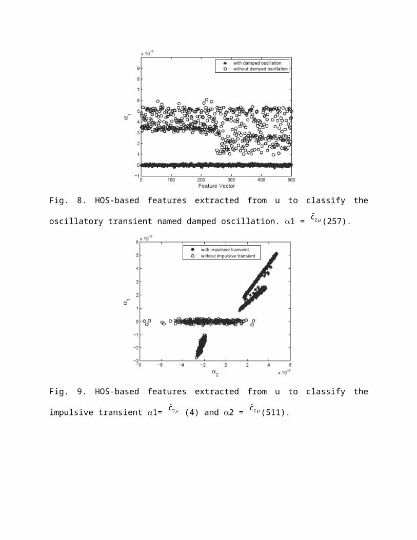
A digital sine-cosine generator is presented in [11]. It can be implemented using the following state equations:

(8)

where s1(n) is a sine function and s2(n) is a cosine function, and the initial states must be correctly set.

The advantage of this approach is that the sine and cosine signal can be used at the same time in both, decomposition and reconstruction tasks.

Figure 4 presents the block diagram of the core structure that extracts the hth harmonic. For extracting N harmonics it is necessary to employ N cores as shown in Fig.4. The advantage of this structure can be summarized as following:

i) low computational effort, suitable for real time decomposition implementation;ii) no phase delay;iii) transient time of only one cycle.

The disadvantage of this structure comes from the limitation of the DFT:

i) a synchronous sampling is needed;ii) interharmonics produce estimation error of the quadrature components.

Fig.4- The core structure for extracting the hth harmonic.

12. 4 Simulation results

In order to present some results of tracking time-varying harmonics using the structure shown in Fig. 4, two examples are considered: (a) a synthetic signal, which has been generated in Matlab using a mathematical model, and (b) a signal obtained from the “Electromagnetic

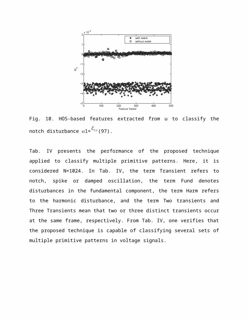
Transient Program including DC systems” (EMTDC) with its graphical interface known as “Power Systems Computer Aided Design” (PSCAD). This program can simulate power systems with high fidelity and the resulting signals of interest are very close to physical reality.

12.4.1 Synthetic Signal

The synthetic signal utilized can be represented by:

(8)

Where h is the order (1st up to 15th) and A is the magnitude of the component; 0 is the fundamental frequency; and finally, f(t) and g(t) are exponential functions (crescent, de-crescent or alternated one) or simply a constant value . Besides, x(t) is portioned in four different segments in such way that the generated signal is a distorted one with some harmonics in steady-state and others varying in time, including abrupt and modulated change of magnitude and phase, as well as a DC component. Figure 5 illustrates the synthetic signal.

Fig. 5 – Synthetic signal used.

The structure composes of 16 cores like Fig. 4 has been used to decompose the signal into sixteen different harmonic orders, including the fundamental (60 Hz) and the DC component.

Figure 6 shows the decomposed signal from 4th up to 7th harmonic components. The left column represents the original components and the right column the corresponding components obtained through the filter bank. For simplicity and space limitation the other component are not shown. However, it is important to remark that all waveforms of the time-varying harmonics are extracted with efficiency along the time.

Naturally, intrinsic transients will be present during the transitions from previous to the new state. Figure 7 shows both the original and the estimated components (DC to 3rd harmonic) in a short time scale interval. The transient of one cycle is shown in each output.

12.4. 2 Simulated Signal It is well known that during energization a transformer can draw a large current from the supply system, normally called inrush current, whose harmonic content is high.

Although today’s power transformers have lower harmonic content, Table 1 shows the typical harmonic components present in the inrush currents [12]. These values are normally used as reference for protection reasons, but they do not take into account the time-varying nature of this phenomenon.

Table 1- typical harmonic content of the inrush current

Order Content %

Dc 552 633 26.84 5.15 4.16 3.77 2.4

0 1 2 3 40

1

2DC component

0 1 2 3 40

1

2DC component

0 1 2 3 4-10

11st

0 1 2 3 4-10

11st

0 1 2 3 4-1

0

12nd

0 1 2 3 4-1

0

12nd

0 1 2 3 4-1

0

13rd

Time s0 1 2 3 4

-1

0

13rd

Time s

0 1 2 3 4-1

0

14th

0 1 2 3 4-1

0

14th

0 1 2 3 4-0.5

0

0.55th

0 1 2 3 4-0.5

0

0.55th

0 1 2 3 4-0.2

00.2

6th

0 1 2 3 4-0.2

00.2

6th

0 1 2 3 4-0.5

0

0.57th

Time s0 1 2 3 4

-0.5

0

0.57th

Time s

0 1 2 3 4-1

0

18th

0 1 2 3 4-1

0

18th

0 1 2 3 4-0.2

00.2

9th

0 1 2 3 4-0.2

00.2

9th

0 1 2 3 4-1

0

110th

0 1 2 3 4-1

0

110th

0 1 2 3 4-0.5

0

0.511th

Time s0 1 2 3 4

-0.5

0

0.511th

Time s

Fig. 6 – First column: original components, second column: decomposed signals.

2.99 3 3.01 3.02 3.03 3.04 3.050

1

2DC component

2.99 3 3.01 3.02 3.03 3.04 3.05-1

0

12nd

2.99 3 3.01 3.02 3.03 3.04 3.05-1

0

13rd

2.99 3 3.01 3.02 3.03 3.04 3.05-0.5

0

0.57th

Time s

Fig. 7 – Comparing original and decomposed component.

In recent years, improvements in materials and transformer design have lead to inrush currents with lower distortion content [13]. The magnitude of the second harmonic, for example, has dropped to approximately 7% depending on the design [14]. But, independent of these new improvements, it is always important to emphasize the time-varying nature of the inrush currents.

In being so, a transformer energization case was simulated using EMTDC/PSCAD, and the result is shown in Fig.8.

Fig. 8 – Inrush current in phase A.

Using the methodology proposed to visualize the inrush current, the Fig.9 reveals the rarely seen time-varying behavior of the waveform of each harmonic component. This could be used to understand other physical aspects not observed previously. In Fig. 9, the left column shows

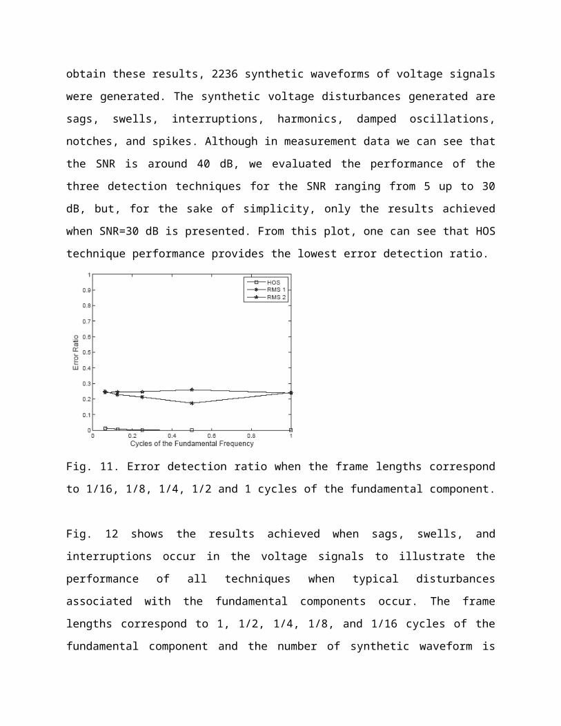
the DC and even components and the right column the odd components.

Fig. 9 – Decomposition of the simulated transformer inrush current.

12.5 ConclusionsThis chapter presents a method for time-varying harmonic decomposition based on sliding

window DFT. The technique is able to extract each harmonic in the time domain. The methodology has as advantages low computation burden, no phase delay and a short transient time and can be used as a useful tool for real time applications. The disadvantages are inherent to all DTF based algorithm, i.e., need synchronous sampling and is influenced by the presence of interharmonics. However some strategies can be used to guarantee synchronization, such as the use of the Phase Looked Loop (PLL) to estimate the fundamental frequency. The influence of the interharmonics can be minimized through the choice of other windows, with smaller Main Lobe width and higher Side-Lobe Attenuation. The cost to be paid is the increasing of the computational effort.

12. 6 References

[1] Yuhua Gu, M. H. J. Bollen, “Time-Frequency and Time-Scale Domain Analysis,” IEEE Trans. on Power Delivery, Vol. 15, No. 4, Oct. 2000, pp. 1279-1284.

[2] P.P. Vaidyanathan, Multirate Systems and Filter Banks, Prentice Hall, 1993.

[3] M. Karimi-Ghartemani, M. Mojiri and A. R. Bakhsahai, “A Technique for Extracting Time-Varying Harmonic based on an Adaptive Notch Filter,” Proc. of IEEE Conference on Control Applications, Toronto, Canada, Aug. 2005.

[4] J. R. Carvalho, P. H. Gomes, C. A. Duque, M. V. Ribeiro, A. S. Cerqueira, and J. Szczupak, “PLL based harmonic estimation,” IEEE PES conference, Tampa, Florida-USA, 2007

[5] H. Sun, G. H. Allen, and G. D. Cain, “A new filter-bank configuration for harmonic measurement,” IEEE Trans. on Instrumentation and Measurement, Vol. 45, No. 3, June 1996, pp. 739-744.

[6] C.-L. Lu, “Application of DFT filter bank to power frequency harmonic measurement,” IEE Proc. Gener. , Transm,. Distrib., Vol 152, No. 1, Jan. 2005, pp. 132-136.

[7] P. M. Silveira, M. Steurer, .P F. Ribeiro, “Using Wavelet decomposition for Visualization and Understanding of Time-Varying Waveform Distortion in Power System,” VII CBQEE, Aug. 2007, Brazil.

[8] V.L. Pham and K. P. Wong, “Antidistortion method for wavelet transform filter banks and nonstationay power system waveform harmonic analysis,” IEE Proc. Gener., Transm., Distrib., Vol 148, No. 2, March 2001, pp. 117-122.

[9] C. A. Duque, P. M. Silveira, T. Baldwin, and P. F. Ribeiro, “Novel method for tracking time-varying power power harmonic distortion without frequency spillover,” IEEE 2008 PES, July 2008, Pittsburgh, PA, USA.

[10] Sanjit K. Mitra, Digital Signal Processing – A computer-based approach, Mc-Graw Hill 2006, 3ª Edition.

[11] R. Hartley, K. Welles, “Recursive Computation of the Fourier Transform", IEEE Int. Symposium on Circuits and Systems, Vol.3, 1990. pp. 1792 -1795.

[12] C.R. Mason, The Art and Science of Protective Relaying, John Wiley & Sons, Inc. New York, 1956.

[13] B. Gradstone, “Magnetic Solutions, Solving Inrush at the Source”, Power Electronics Technology, April 2004, pp 14-26.

[14] F. Mekic, R. Girgis, Z. Gajic, E. teNyenhuis, “Power Transformer Characteristics and Their Effect on Protective Relays”, 33rd Western Protective Relay Conference, Oct. 2006.