View Publications online（PDF／780KB）

Empirical Study of Growth and Poverty Reduction in Indonesian Farms:

The Role of Space, Infrastructure and Human Capital and Impact of the

Financial Crisis

Human Capital, Mobility, and Income

Dynamics: Evidence from Indonesia

No. 11

March 2010

Reno Dewina and Futoshi Yamauchi

Use and dissemination of these working papers are encouraged; however, the JICA Research Institute requests due acknowledgement and a copy of any publication for which these working papers have provided input. The views expressed in these papers are those of the author(s) and do not necessarily represent the official positions of either the JICA Research Institute or JICA. JICA Research Institute 10-5 Ichigaya Honmura-cho Shinjuku-ku Tokyo 162-8433 JAPAN TEL: +81-3-3269-3374 FAX: +81-3-3269-2054 Copyright ©2010 by Japan International Cooperation Agency Research Institute All rights reserved.

1

Human Capital, Mobility, and Income Dynamics

Evidence from Indonesia

Reno Dewina* and Futoshi Yamauchi

Abstract

This paper examines the effects of household formation on income dynamics using panel data

from Indonesia. The focus of our analysis is to explore the determinants of household income

dynamics in 1995-2007 when we change the definition of household. Empirical results show

that intergenerational gap in education (i.e., education growth) as well as the number of young

and prime-age members in the household play important roles in determining income dynamics,

especially when we include out-migrants. This is consistent with individual migration behavior:

the young and educated tend to move out of their villages over the 12 years. We also found that

out-migration increases net-remittances to the household. The results indicate the importance of

human capital as well as endogenous migration (attrition) in rural household income dynamics.

Keywords: Income Dynamics, Human Capital, Migration, Split, Indonesia

* International Food Policy Research Institute, Washington D.C. International Food Policy Research Institute, Washington D.C. ([email protected]) We are grateful to Jaime Quizon, Nick Minot, Homi Kharas, Megumi Muto, Takako Yuki, Ali Subandoro, Sony Sumaryanto, and seminar participants at the Indonesian Ministry of Agriculture for useful comments. Research findings of this paper are based on collaboration between the Japan International Cooperation Agency, the International Food Policy Research Institute, and the Indonesian Center for Agriculture and Socio Economic Policy Studies. Any remaining errors are ours.

2

Introduction

Income and human resource mobility are interlinked in situations where agricultural

growth faces a limitation due to scare land, and high-return activities are concentrated in urban

areas and the non-agricultural sector. Under such a circumstance, potential efficiency gains from

mobilizing resources from rural to urban areas is large, particularly when the gap in economic

growth between agriculture and non-agriculture is large.

In this situation, migration to urban sectors has a direct implication for income

dynamics in rural households as the migrants tend to remit a substantial portion of their income

to their rural origins or play an important role to pool income shocks between extended families

(e.g., Lucas and Stark 1985; Rosenzweig and Stark 1989). Therefore, whether migrants are

included in the computation of household incomes (even though they live in urban areas) makes

a difference in the dynamic analysis of household income and mobility, given that individual

mobility is an endogenous decision. In this paper, we examine mechanisms that govern

individual migration behavior with a clear linkage to household income dynamics using panel

data from Indonesia.

Labor markets are likely to be segmented by schooling levels. According to Otsuka and

Yamano (2006), educated workers in rural Asia tend to find lucrative non-farm jobs, whereas

uneducated workers tend to engage in relatively low-paying jobs including hired labor in the

agricultural sector. Also, it is important to note from their panel studies in Asia that increased

agricultural income, mostly generated from the Green Revolution, was likely to be a major

source of funds to invest in children’s education in the early years, which later led to the choice

of nonfarm occupations by children. The modern agricultural technology and human capital

acquired through schooling are two important factors that affected the growth of household

income and poverty reduction in rural areas (Cherdchuchai and Otsuka 2006). A question arises

as to what will occur to rural households once such technological opportunities cease.

3

Our empirical study comes from panel data in Indonesia. In this country, the limited

supply of natural resources such as land has often been seen as a major constraint of farm

income growth. The majority of farmers are smallholders or agricultural laborers, especially in

Java. The scarcity of land, particularly on Java, forces household members to seek off-farm

work opportunities. Moreover, when employment opportunities in non-agricultural sectors are

growing in general, it creates large incentives for rural households to out-migrate and/or supply

their labor to non-agricultural sectors. From data that we collected in 7 provinces in 2007, we

found that the average cultivated land sizes in Java and non-Java are 0.37 and 0.73 hectares

respectively.1 This shows the difficulty with relying solely on the agriculture sector in the long

run, since agricultural growth depends heavily on land availability. Based on the 1993

Agriculture Census, the average land size in the country was 0.86 hectares, where 49 percent of

households had less than 0.5 hectares in land holdings (Supadi and Susilowati 2004).2 Under

the circumstance, investment in human capital is an important element to alleviating poverty in

rural areas.

Using the same sample used in this study, Yamauchi (2008) shows that there has been

significant growth in educational attainment in the rural population, promoting transitions from

agriculture to non-agriculture over time. Intergenerational gap in education within the household

changes household’s income prospects. In this paper, we investigate the implications of

education growth on household income growth and split/migration behavior. To capture

incomes of out-migrants, we simulated their incomes using the information on individual

characteristics such as age, gender and education. The analysis shows that higher education

growth (more years of schooling in the young generation against the old generation) increases

the total household income growth with more out-migrants moving out of their villages.

1 These figures are based on our sample (discussed in Section 3). 2 For example, the average land sizes are smaller than those of the Philippine and Thailand studies cited above (Estudillo et al, 2006; Cherdchuchai and Otsuka, 2006). In the Philippines the average farm size was 1.3 and 1.0 hectare in 1985 and 2004 respectively while it was 6.3 and 5.8 hectares in 1987 and 2004 respectively in Thailand (two provinces).

4

Our approach also addresses attrition bias in panel analysis (e.g., Rosenzweig 2003;

Thomas et al. 2001). Household composition is endogenous because household members decide

their locations over time. Moreover, the division of the household has implications on the

division of household public goods and income dynamics (Foster and Rosenzweig 2002).

Therefore, the computation of household income also depends on who (we think) are members

of the household. We do not directly try to correct attrition bias in the analysis of income

dynamics, but we compare estimated returns to the initial assets such as schooling and land by

changing the definition of household composition, by including split members and out-migrants.

In the analysis below, we have two overlapping issues. First, household members

dynamically decided whether they stay or move out of the household. Second, in research, we

also must define the household, taking into account both data limitations and research objectives.

In this paper, we will check how such decisions, made by agents and researchers, affect

empirical estimates of income dynamics.

The paper is organized as follows. The next section discusses our empirical approach.

In Section 3, we describe our survey and data.

Section 4 summarizes empirical results. First, the intergenerational gap in education in

the household increases household income if we include simulated incomes of out-migrants.

Land shows diminishing returns in the rural areas, but increases the above-mentioned dynamic

effect of education growth on income growth. The number of household members, especially

prime-age groups, also significantly increases income growth. Therefore, both the quality and

quantity of human capital in the initial period have dynamic returns.

Second, the analysis of individual mobility supports the above findings - the more

educated and young are more likely to move out of the village. Land also helps agents migrate.

Females tend to split from the household (staying in the same village), while males tend to

migrate out of the village. Third, net remittance increases as the number of out-migrants

increases. Overall, these results from income dynamics, mobility and remittances are consistent.

5

2. Empirical method

We estimate growth equations with income growth as the dependent variable regressed

on initial conditions. In our exercise, we explicitly take into account the endogenous nature of

income growth as a function of demographic dynamics. That is, income growth depends on

changes in household composition over time. In particular, migration and household split are

important in our analysis.

The equation we estimate is as follows.

1( )i it i iy z X (1)

where y is income growth, X is a set of the initial conditions, and z is demographic

conditions. Income growth as a function of demographic conditions is

2 1 2 2 1 1( , ) ( ) ( )i i i i i i iy z z y z y z . (2)

We construct different measures of income growth by using different definitions of the

household: household members residing in the original households, plus household members

who split from the original households but reside in the same villages, plus out-migrants who

moved out of the original households and not residing in the villages. Returns to household

characteristics depend on migration behavior and the definition of household in period 2.

To provide micro-foundations for the above income dynamics, we also analyze

individual-level dynamic mobility: staying in the original households, split or out-migrate.

Below k is the index to define individual location; k=1 original, =2 split, and =3 out-migrate.

By definition, in the initial period, k=1 for all.

6

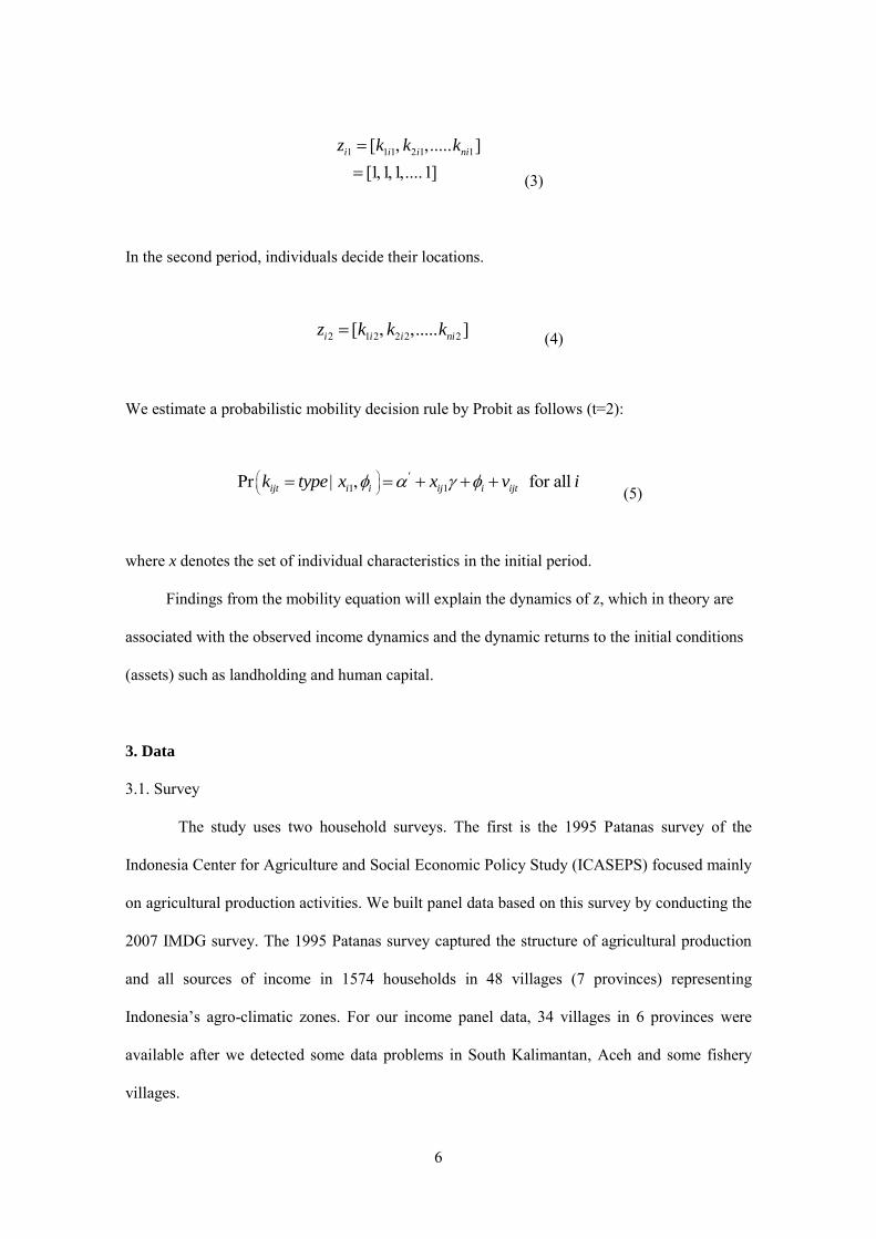
1 1 1 2 1 1[ ][1 1 1 1]

i i i niz k k k

(3)

In the second period, individuals decide their locations.

2 1 2 2 2 2[ ]i i i niz k k k (4)

We estimate a probabilistic mobility decision rule by Probit as follows (t=2):

1 1Pr for allijt i i ij i ijtk type x x v i

(5)

where x denotes the set of individual characteristics in the initial period.

Findings from the mobility equation will explain the dynamics of z, which in theory are

associated with the observed income dynamics and the dynamic returns to the initial conditions

(assets) such as landholding and human capital.

3. Data

3.1. Survey

The study uses two household surveys. The first is the 1995 Patanas survey of the

Indonesia Center for Agriculture and Social Economic Policy Study (ICASEPS) focused mainly

on agricultural production activities. We built panel data based on this survey by conducting the

2007 IMDG survey. The 1995 Patanas survey captured the structure of agricultural production

and all sources of income in 1574 households in 48 villages (7 provinces) representing

Indonesia’s agro-climatic zones. For our income panel data, 34 villages in 6 provinces were

available after we detected some data problems in South Kalimantan, Aceh and some fishery

villages.

7

The 2007 IMDG was a general household survey designed to capture a variety of

household activities. We planned to expand the sample by adding 51 new villages in the 7

provinces. In the revisited villages, we resampled 20 households per village from the original

1995 Patanas sample (proportionally with their landholding size) and tracked their split

households. In the new villages, we sampled 24 households from two main hamlets in each

village to proportionally represent landholding distribution. Since we were not able to revisit

one of the original Patanas villages in NTB for safety reasons, in 2007, we had 47 revisited and

51 new villages. Thus, the total sample consists of 2,266 households from 98 villages in 7

provinces.

3.2. Income construction in 2007

Income is calculated in both surveys as the sum of net earnings from agriculture and

non-agriculture sources. In our analysis, we do not include transfer incomes as our focus is on

(labor) earnings. However, we include the imputed out-migrant incomes when the definition of

income requires so. The sources are from the following sources: crop production, livestock

production, non-agriculture employment, self employment, agriculture employment and other

incomes.

The crop production covers the three crop seasons and a non season during the past one

year. It is calculated from different sources: food crops, sugar cane and estate plant/home garden.

The value of production is obtained by multiplying the total production quantities with the

selling price per unit of each crop. We also include the production value if households market

their produce through Ijon and Tebasan systems3. Crop production cost includes seeds, fertilizer,

pesticides, supporting materials, irrigation, land rental, land tax, marketing, transportation and

3Ijon is a method by which farmers obtain loans from buyers (traders). The farmer sells his crop long before harvest at a price that is usually quite low relative to the regular market price at harvest time. The buyer is responsible for protecting the crop from pests and thieves, and bears the costs of harvesting and transportation. The method is similar to Tebasan, except for the fact that in Ijon, farmers sell much before harvest.

8

others. After aggregating the crop production values and crop costs by household, we calculated

the net income by deducting production costs from production value.

Livestock is differentiated into poultry, quail and duck, broiler, ruminant and dairy. The

livestock revenue includes the value of livestock sold, home consumption of the animal meat

and by-products such as egg and milk. The net income is obtained by deducting the input costs

(seeds, feed, medicine and supplements, and labor cost) and marketing costs (processing and

transportation cost).

Aquaculture income covers the fish pond from three different cycles and marine fishery

from peak, normal and slack seasons. The net income is obtained by calculating the sales of

products and by products minus the production costs and marketing cost.

The non-farm employment income is calculated from the non-agriculture employment

section in the questionnaire. The module captures employment incomes from the past one year,

both in-cash and in-kind. The net income is calculated by deducting the expenses from the gross

revenue.

Other sources of non-farm income are self-employment work. This reflects any earnings

of household members who involved in the self employed business activities monthly. The net

income from self-employment by nonfarm enterprises can be directly calculated as the total of

gross revenue minus expenses.

The agriculture employment section excludes the work on own farm. The net income is

the agricultural labor income minus expenses (transportation costs). For other non-employment

sources, since we only consider household earnings, we exclude transfer income.

As we confirm later in individual migration equations, with better income prospects the

young and educated are likely to move out of the sample villages. Therefore, in our hypothesis,

we conjecture that returns to human capital will be biased downward if we omit this group of

household members who moved out in 1995-2007.

The 2007 survey collected information on out-migrants’ activities, but not their incomes.

9

From the survey, we know their main activity, occupation, industry, marital status and location.

To simulate their incomes, we use a standard log-wage equation4 with the estimates: 0.067 for

years of schooling, 0.0425 for male indicator, 0.0811 for age, and 0.008 for age squared. For the

constant term, we used log of 700,000 so that the mean of simulated wage distribution is

matched to the average earnings in West Java (including Jakarta) in 2006.5

For the purpose of analysis, we categorized individual members into three different

groups, which are (i) stayers (for members who stay in the original household), (ii) splitters (for

members who moved into different house but still in the village; and (iii) out-migrants

(members who left the original household and migrated).

We can compute per capita income growth in three cases: households in 2007 include only (i)

Group 1: stayers, (ii) Group 2: stayers and splitters, and (iii) Group 3: stayers, splitters and

out-migrants. To compute per capita income, we identify the number of household members

between ages of 15 to 65. The mean per-capita income growth in 1995-2007 is 1.55, 1.60, and

2.01 for Groups 1, 2 and 3, respectively. Table 1 shows summary statistics of key

demographic variables for each group.

Table 1. Age, schooling and gender among stayers, splitters and out-migrants

Stayers Splitters Out-migrants Age

28.0

23.4

17.6

Years of schooling

4.8

5.9

5.8 HH member age 15 or less HH member age 15-29 HH member age 30-44 HH member age 45-64 HH member age 65 or older Gender Male

2.8

7.2

5.3

4.4

2.4

0.5

3.7

10.7

4.4

3.7

1.2

0.5

4.4

8.7

5.5

3.9

2.4

0.4 4 Mincer equation: edXcXbSay 2log , S for schooling and X for experience 5 We used Nominal Wage of Manufacturing Workers by Region, 2004-2006 (September'06 average), available in Statistics Indonesia (http://www.bps.go.id/sector/wages/table2.shtml)

10

Source: IMDG 2007 and 1994/95 Patanas

Out-migrants have very different characteristics in term of their age and years of

schooling than other two groups. The out-migrants, on average, show the lowest age among

them and similar level of years of schooling with splitters. This implies that these young people

with higher education tend to seek better opportunities by migrating from their home village.

Another interesting finding is that the splitters have the lowest education and highest average

age. In terms of gender, females are more dominant among out-migrants, but males are the

majority among stayers. When we break down the age of household members, we can see that

in almost all age-category the years of schooling of out-migrant are dominant compared to other

two groups, but in age group 15-30 and 45-64.

4. Empirical results

4.1. Income dynamics

This section summarizes empirical results on income dynamics. Our interest is to

compare returns to household assets, mainly human capital and land, when we change the

definition of household composition, including only original household members, also split

members, and out-migrants. For this purpose, we constructed income measures depending on

the household definition. For the analysis, we focus on per-capita income growth, in order to

include changes in the total income and household compositions.

11

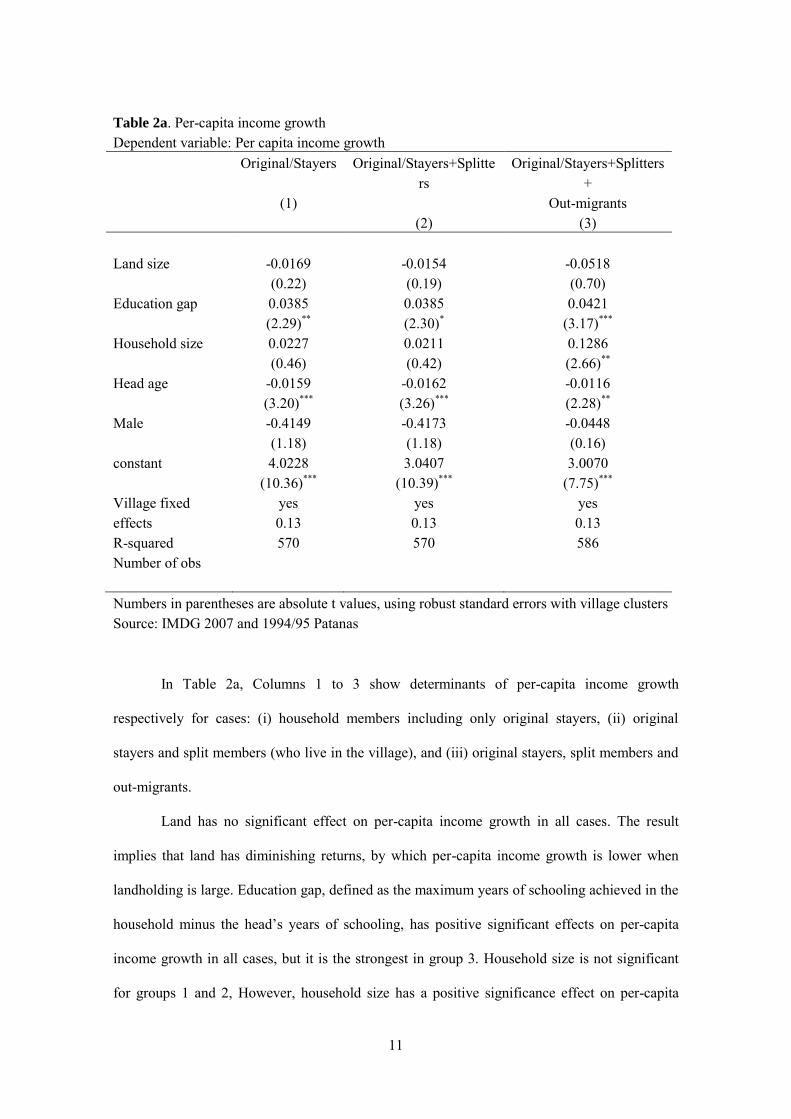
Table 2a. Per-capita income growth Dependent variable: Per capita income growth Original/Stayers

(1)

Original/Stayers+Splitters

(2)

Original/Stayers+Splitters+

Out-migrants (3)

Land size Education gap

-0.0169 (0.22)

0.0385 (2.29)**

-0.0154 (0.19) 0.0385 (2.30)*

-0.0518 (0.70) 0.0421

(3.17)***

Household size Head age

0.0227 (0.46)

-0.0159 (3.20)***

0.0211 (0.42)

-0.0162 (3.26)***

0.1286 (2.66)**

-0.0116 (2.28)**

Male constant Village fixed effects R-squared Number of obs

-0.4149 (1.18) 4.0228

(10.36)***

yes 0.13 570

-0.4173 (1.18) 3.0407

(10.39)***

yes 0.13 570

-0.0448 (0.16) 3.0070

(7.75)***

yes 0.13 586

Numbers in parentheses are absolute t values, using robust standard errors with village clusters Source: IMDG 2007 and 1994/95 Patanas

In Table 2a, Columns 1 to 3 show determinants of per-capita income growth

respectively for cases: (i) household members including only original stayers, (ii) original

stayers and split members (who live in the village), and (iii) original stayers, split members and

out-migrants.

Land has no significant effect on per-capita income growth in all cases. The result

implies that land has diminishing returns, by which per-capita income growth is lower when

landholding is large. Education gap, defined as the maximum years of schooling achieved in the

household minus the head’s years of schooling, has positive significant effects on per-capita

income growth in all cases, but it is the strongest in group 3. Household size is not significant

for groups 1 and 2, However, household size has a positive significance effect on per-capita

12

income growth for group 3. Having large household size gives two impacts, static and

dynamic effects. In the static setting, the larger household size will lower per-capita income

growth since it would increase the denominator. The dynamic effect is quite different, as a large

family can send more members to activities outside the village. Our findings show that

household size seems to have a positive dynamic effect on per-capita income growth.

Household head’s age is significantly negative in all cases. This implies that older

cohorts, defined by the head’s age, do not increase per-capita income growth.

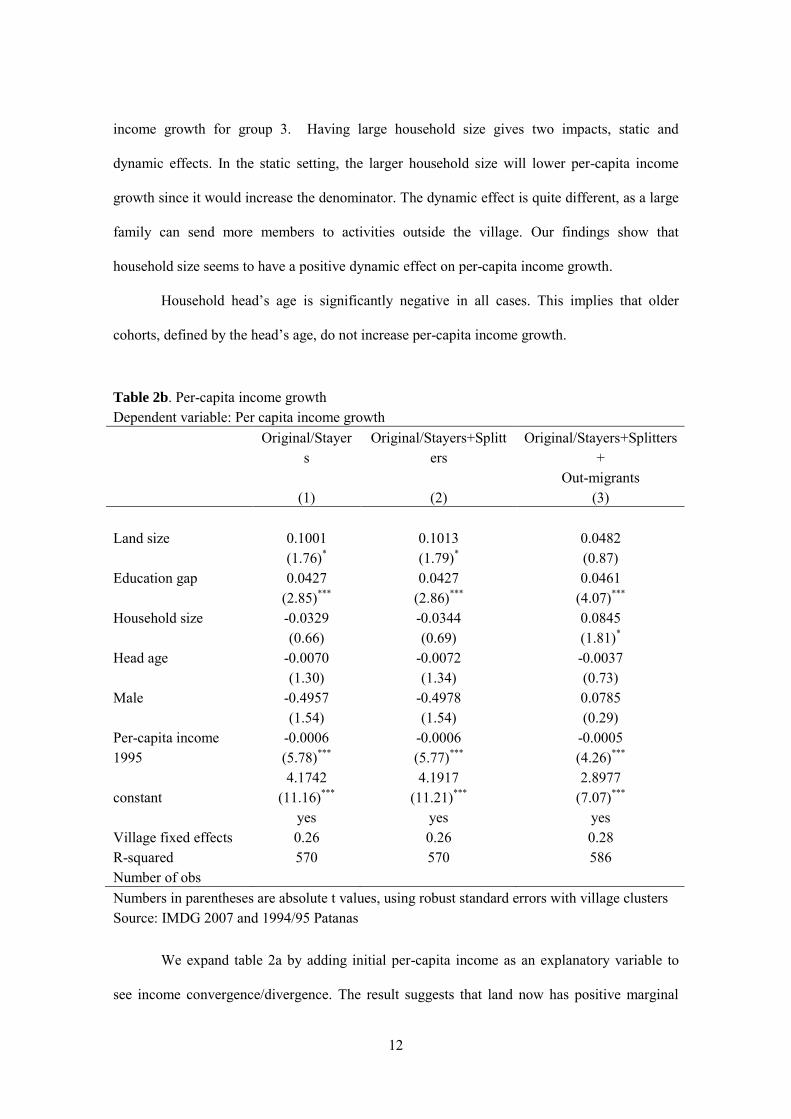
Table 2b. Per-capita income growth Dependent variable: Per capita income growth Original/Stayer

s

(1)


(2)


Out-migrants (3)


0.1001 (1.76)*

0.0427 (2.85)***

0.1013 (1.79)*

0.0427 (2.86)***

0.0482 (0.87) 0.0461

(4.07)***

Household size Head age

-0.0329 (0.66)

-0.0070 (1.30)

-0.0344 (0.69)

-0.0072 (1.34)

0.0845 (1.81)*

-0.0037 (0.73)

Male Per-capita income 1995 constant Village fixed effects R-squared Number of obs

-0.4957 (1.54)

-0.0006 (5.78)***

4.1742 (11.16)***

yes 0.26 570

-0.4978 (1.54)

-0.0006 (5.77)*** 4.1917

(11.21)***

yes 0.26 570

0.0785 (0.29)

-0.0005 (4.26)*** 2.8977

(7.07)***

yes 0.28 586


We expand table 2a by adding initial per-capita income as an explanatory variable to

see income convergence/divergence. The result suggests that land now has positive marginal

13

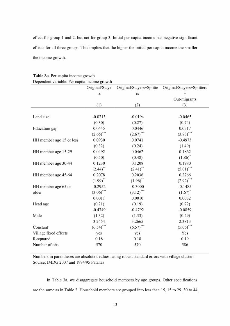
effect for group 1 and 2, but not for group 3. Initial per capita income has negative significant

effects for all three groups. This implies that the higher the initial per capita income the smaller

the income growth.

Table 3a. Per-capita income growth Dependent variable: Per capita income growth Original/Staye

rs

(1)


(2)


Out-migrants (3)


-0.0213 (0.30)

0.0445 (2.65)***

-0.0194 (0.27) 0.0446

(2.67)***

-0.0465 (0.74) 0.0517

(3.83)***

HH member age 15 or less HH member age 15-29 HH member age 30-44 HH member age 45-64 HH member age 65 or older Head age Male Constant

0.0930 (0.32) 0.0492 (0.50) 0.1230 (2.44)**

0.2078 (1.99)**

-0.2952 (3.06)***

0.0011 (0.21)

-0.4749 (1.32) 3.2454

(6.54)***

0.0741 (0.24) 0.0462 (0.48) 0.1208 (2.41)**

0.2036 (1.96)**

-0.3000 (3.12)***

0.0010 (0.19)

-0.4792 (1.33) 3.2665

(6.57)***

-0.4973 (1.49)

0.1862 (1.86)*

0.1980 (5.01)***

0.2766 (2.92)***

-0.1485 (1.67)*

0.0032 (0.72)

-0.0859 (0.29) 2.3813

(5.06)***

Village fixed effects R-squared Number of obs

yes 0.18 570

yes 0.18 570

Yes 0.19 586


In Table 3a, we disaggregate household members by age groups. Other specifications

are the same as in Table 2. Household members are grouped into less than 15, 15 to 29, 30 to 44,

14

45 to 64, and above 65. We found that prime-age groups, those of ages 30 to 64 in 1995,

significantly contribute to the per-capita income growth. The effects become larger in Column 3

(i.e., we include out-migrants). The effect of members aged 15 to 29 is also significantly

positive when we include out-migrants. The elderly group, which is group of age 65 and older,

has negative significant effect on per capita income growth. The effect for group 3 is less

significant compared to other groups though. This makes sense since the contribution from

older people in urban area is assumed much smaller than the prime age group. This is because

the nature of work in urban area is usually suited for prime age group with adequate skills and

education. These findings are consistent with our hypothesis that household size has a dynamic

effect on income growth through migration, and such effects are supposed to be largest if they

have prime-age adult members.

Our previous results on education gap and land remain the same. Interestingly, the effect

of education gap is the largest in Column 3. That is, educational attainment in the young

generation relative to the head has the largest effect on income growth if they have migration

opportunities.

15

Table 3b. Per-capita income growth Dependent variable: Per capita income growth Original/Staye

rs

(1)


(2)

Original/Stayers+ Splitters+

Out-migrants (3)


0.0759 (1.34)

0.0418 (2.76)***

-0.0765 (1.36) 0.0420

(2.80)***

0.0344 (0.70) 0.0494

(4.15)***

HH member age 15 or less HH member age 15-29 HH member age 30-44 HH member age 45-64 HH member age 65 or older Head age Male Per-capita income 1995 Constant

0.1428 (0.41)

-0.0689 (0.75) 0.0215 (0.40)

0.1448 (1.51)

-0.1691 (1.99)**

-0.0013 (0.23)

-0.5115 (1.54)

-0.0005 (5.15)***

3.6686 (8.20)***

0.1337 (0.37)

-0.0701 (0.78) 0.0196 (0.36)

0.1406 (1.48)

-0.1736 (2.05)**

-0.0011 (0.20)

-0.5522 (1.54)

-0.0006 (5.13)*** 3.6832

(8.25)***

-0.4288 (1.13)

0.0759 (0.79)

0.1175 (2.94)***

0.2372 (2.82)***

-0.0338 (0.44)

0.0033 (0.74) 0.0622 (0.22)

-0.0005 (4.24)***

2.5218 (5.50)***


yes 0.27 570

yes 0.27 570

Yes 0.30 586


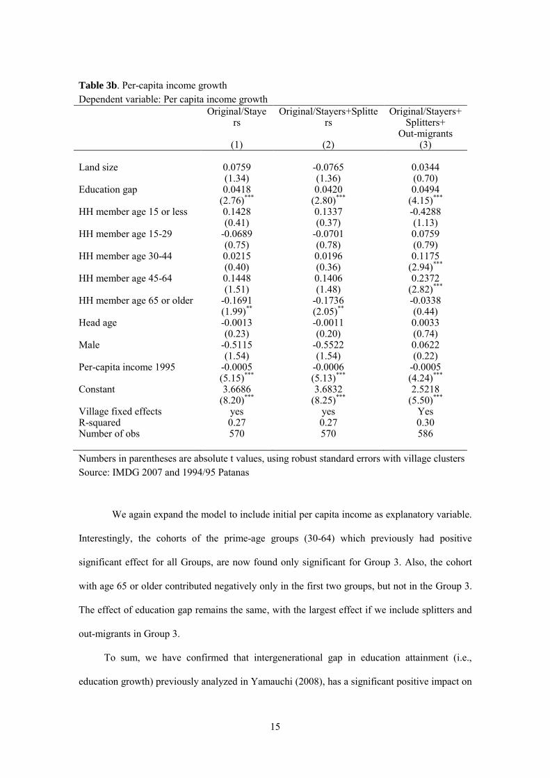
We again expand the model to include initial per capita income as explanatory variable.

Interestingly, the cohorts of the prime-age groups (30-64) which previously had positive

significant effect for all Groups, are now found only significant for Group 3. Also, the cohort

with age 65 or older contributed negatively only in the first two groups, but not in the Group 3.

The effect of education gap remains the same, with the largest effect if we include splitters and

out-migrants in Group 3.

To sum, we have confirmed that intergenerational gap in education attainment (i.e.,

education growth) previously analyzed in Yamauchi (2008), has a significant positive impact on

16

income growth, and its effect is augmented if we include out-migrants in the definition of

household. Also household size shows a significant effect on per-capita income growth

dynamics. The size plays an important role in influencing the per-capita income growth, and

more importantly the household composition matters. An increase in the proportion of members

aged 15 to 64 significantly increases the household income growth, and its effect becomes

larger if we include out-migrants. In the next section, we investigate factors determining the

likelihood of household division and migration.

4.2. Mobility and household division

In this section, we estimate individual-level mobility equations to identify determinants

of household division and migration. The estimation adopts multinomial logit, using the original

household stayers as the omitted benchmark case. Explanatory variables are taken from the

1995 Patanas survey6. Preliminary analysis shows a small number of splitters who set up new

households in the sample villages, which implies that they are likely to merge with other new

members to start new households (such as marriage). Out-migrants head to urban labor markets.

The proportion of male is slightly dominant in stayers and splitters (52.1%), not for

out-migrants (46%). The average age is quite close between the first and second member type

(stayers and splitters) which is 29 and 31 years, respectively, but it is much younger (18 years)

for the third type (outmigrants). Years of schooling is highest among out-migrants (9 years),

followed by splitters and stayers, at 8 and 6 years respectively. For the equation estimating

individual level mobility, we specifically change the definition of education gap, which is now

defined as the own years of schooling achieved from individual member minus the head’s years

of schooling, we define it as education gap (own)

6 We calculated age of schooling in 1995 using 2007 information on schooling history that contains age started and completed schooling, years of schooling completed and details on each education level and grade. Thus, we were able to recover information on schooling in 1995 (which was only available in terms of categorical variable such as unfinished primary school, primary school graduate etc.).

17

Table 4. Individual mobility

Splitters (2)

Out-migrants (3)

Land size

0.1567 (0.87)

0.1496 (2.00)**

Age -0.0520 (3.71)***

-0.1049 (14.60)***

Head years of school 0.0256 (0.33)

0.1720 (5.53)***

Male 0.0732 (0.35)

0.5045 (3.79)***

Education gap 0.2071 (1.96)**

0.2791 (12.95)***

Constant Village dummies Log pseudolikelihood Pseudo R2

-0.0663 (0.15)

Yes -1116.412

0.2776

-0.7974 (3.00)***

Number of obs 2431

Numbers in parentheses are absolute z values, using robust standard errors with village clusters. Source: IMDG 2007 and 1994/95 Patanas

Table 4 summarizes our empirical results. The findings show that (i) the young tend to

split and migrate, and (ii) education gap has a larger effect on the migration probability than

household split. Experience (age) and intergenerational gap in human capital (education) seem

important in explaining household dynamics. Especially, the result on education gap is

consistent with that of income growth, i.e., intergenerational gap in education promotes

out-migration, which significantly increases the total income for the household.

The age effect in household split suggests that marriage is one of important reasons for

individual member to leave their parent house. The results also shows that males tend to split

and migrate more than females. After a certain age, sons/daughters will get married and most

likely will move from their parent house. However, sons are more likely to leave their parents

house and set up a new household.

Land size significantly increases the probability of household out-migration. It implies

18

that large landholding enables the original household to support out-migration probably because

a large landholding makes it easier to finance migration (including study outside the village).

It is worth mentioning that young age and educational attainment are connected with

out-migration, as confirmed in other studies (e.g., Schultz 1982; Schwartz 1976). The reason for

the young to leave the village is not only for entering a labor market but also in order to

complete their schooling. The young people look for opportunities in non-agricultural sector

where they seek income prospects that are better than agriculture. Investment in schooling is a

rewarding method to have this transition. Better education offers other opportunities that they

otherwise cannot find in the village. Although land is one of the most important assets in rural

areas (particularly in agricultural production), land does not necessarily keep them to stay in the

village but actually encourages out-migration. The diminishing returns to land in the Indonesian

agriculture (especially, in Java) might be one of the reasons. These results provide the

foundation for income dynamics analyzed in the previous section.

We assume that spatial connectivity in the local area would have an effect on

migration/mobility. Therefore, in order to observe whether our assumption is correct or not we

have expanded the model in Table 4 and integrated a spatial connectivity variable, which is

represented by change of asphalt road in the local area from 1996-2006, in our explanatory

variables. We added a spatial connectivity variable and interaction of that spatial connectivity

variable with characteristics variables using province dummies to control the bias. The results of

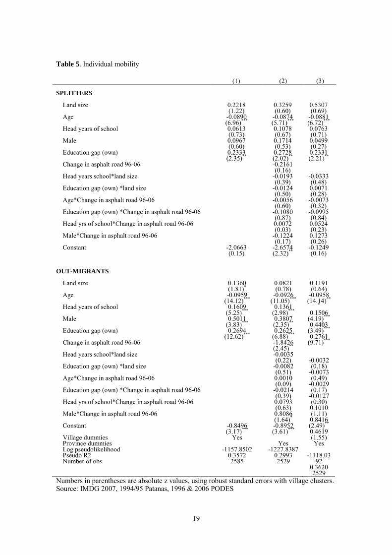
expanded models are shown in Column (2) and (3) of Table 5 respectively.

19

Table 5. Individual mobility

(1)

(2)

(3) SPLITTERS Land size Age

0.2218 (1.22)

-0.0890 (6.96)***

0.3259 (0.60)

-0.0874 (5.71)***

0.5307 (0.69)

-0.0881 (6.72)***

Head years of school Male Education gap (own) Change in asphalt road 96-06 Head years school*land size Education gap (own) *land size Age*Change in asphalt road 96-06 Education gap (own) *Change in asphalt road 96-06 Head yrs of school*Change in asphalt road 96-06 Male*Change in asphalt road 96-06 Constant

0.0613 (0.73) 0.0967 (0.60) 0.2333 (2.35)**

-2.0663 (0.15)

0.1078 (0.67) 0.1714 (0.53) 0.2728 (2.02)**

-0.2161 (0.16)

-0.0193 (0.39)

-0.0124 (0.50)

-0.0056 (0.60)

-0.1080 (0.87) 0.0072 (0.03)

-0.1224 (0.17)

-2.6574 (2.32)**

0.0763 (0.71) 0.0499 (0.27) 0.2331 (2.21)**

-0.0333 (0.48) 0.0071 (0.28)

-0.0073 (0.32)

-0.0995 (0.84) 0.0524 (0.23) 0.1273 (0.26)

-0.1249 (0.16)

OUT-MIGRANTS Land size Age Head years of school Male Education gap (own)

Change in asphalt road 96-06 Head years school*land size Education gap (own) *land size Age*Change in asphalt road 96-06 Education gap (own) *Change in asphalt road 96-06 Head yrs of school*Change in asphalt road 96-06 Male*Change in asphalt road 96-06 Constant Village dummies Province dummies Log pseudolikelihood Pseudo R2 Number of obs

0.1360 (1.81)*

-0.0959 (14.12)***

0.1609 (5.25)*** 0.5011

(3.83)*** 0.2694

(12.62)***

-0.8496 (3.17)***

Yes

-1157.8502 0.3572 2585

0.0821 (0.78)

-0.0926 (11.05)***

0.1361 (2.98)***

0.3807 (2.35)**

0.2625 (6.88)***

-1.8426 (2.45)**

-0.0035 (0.22)

-0.0082 (0.51) 0.0010 (0.09)

-0.0214 (0.39) 0.0793 (0.63) 0.8086 (1.64)*

-0.8952 (3.61)***

Yes

-1227.8387 0.2993 2529

0.1191 (0.64)

-0.0958 (14.14)**

*

0.1506 (4.19)***

0.4403 (3.49)***

0.2761 (9.71)***

-0.0032 (0.18)

-0.0073 (0.49)

-0.0029 (0.17)

-0.0127 (0.30) 0.1010 (1.11) 0.8416 (2.49)**

0.4619 (1.55)

Yes

-1118.0392

0.3620 2529

Numbers in parentheses are absolute z values, using robust standard errors with village clusters. Source: IMDG 2007, 1994/95 Patanas, 1996 & 2006 PODES

20

Basically, spatial connectivity has two different effects on mobility, on one side it spurs

mobility and it stops mobility on the other side. Road quality explains that development of

localized spatial connectivity is important in opening access to greater economic opportunities.

People react on this improvement in two ways, first, better road quality will let people have easy

access moving out from the village considering the opportunities they have outside the village.

Secondly, the improvement of road quality would speed up their trip and people could manage

to commute and remain in the same location. These two different effects might cancel each

other as shown in the regression results. Columns (2) and (3) show that spatial connectivity has

no effect on household division and migration. However, one thing that needs to be noted is that

the interaction of change of the asphalt road and gender is significant for migrants (but not for

splitters). It implies that male members tend to migrate out due to the improvement of the road.

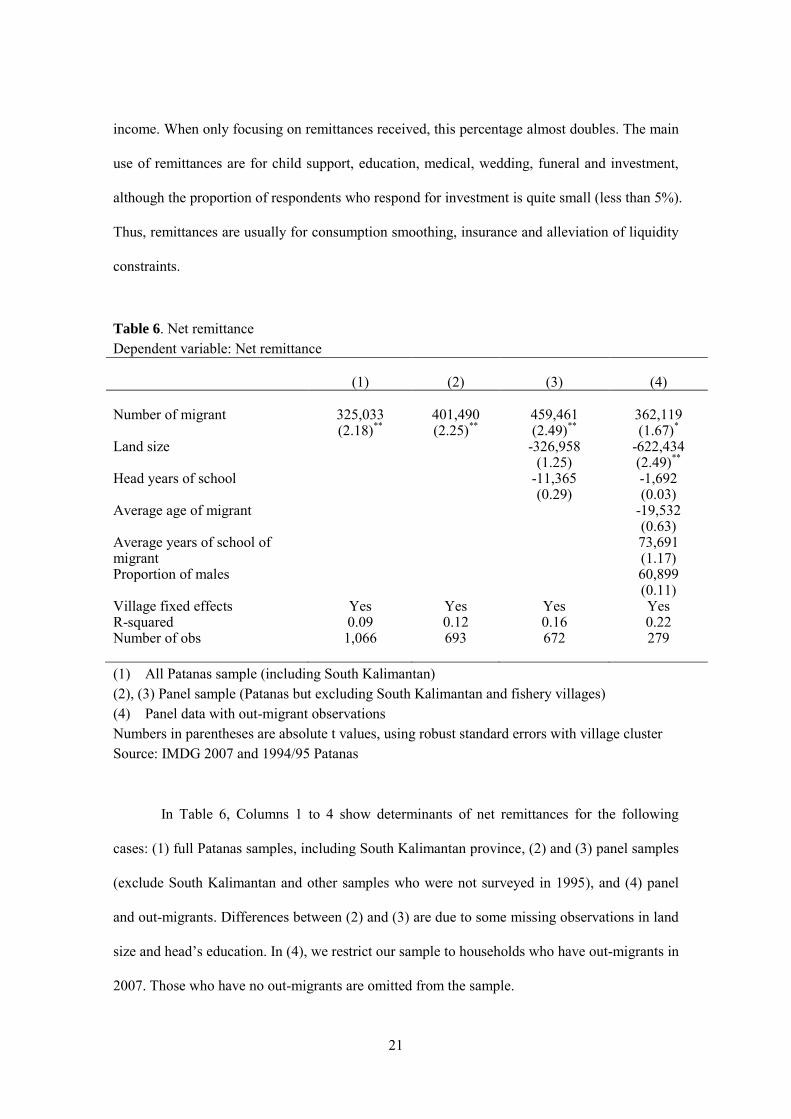
4.3. Remittances

The empirical results in this section report on net remittances. In the analysis, we expect

average net remittances at the household level to be determined by out-migrants characteristics

such as number of out-migrants, land size, household head years of school, average age of

out-migrant, average years of schooling of out-migrant and proportion of male in out-migrant

household. Since we assume that out-migrants who remit are in labor markets, for their

characteristics we include only productive out-migrants (age 15 to 64 years) with working status

(exclude students). Data on remittances include transfers (in/out) in the forms of cash and

in-kind (food and non-food). Most remittances (about 86 percent) are in the form of cash. For

this purpose, we calculated net remittances as remittances received minus the remittances sent

by the households.

About 44.3 percent of household samples are recipients of remittances. The flows of

remittances are mainly among core family members and relatives, accounting for more than 90

percent and small portion going to/from neighbors or friends. The average amount of annual net

remittances is about 700 thousand Rupiahs, which is about 4 percent of average household

21

income. When only focusing on remittances received, this percentage almost doubles. The main

use of remittances are for child support, education, medical, wedding, funeral and investment,

although the proportion of respondents who respond for investment is quite small (less than 5%).

Thus, remittances are usually for consumption smoothing, insurance and alleviation of liquidity

constraints.

Table 6. Net remittance Dependent variable: Net remittance

(1)

(2)

(3)

(4)

Number of migrant Land size Head years of school Average age of migrant

325,033 (2.18)**

401,490 (2.25)**

459,461 (2.49)**

-326,958 (1.25)

-11,365 (0.29)

362,119 (1.67)*

-622,434 (2.49)**

-1,692 (0.03)

-19,532 (0.63)

Average years of school of migrant

73,691 (1.17)

Proportion of males

60,899 (0.11)


Yes 0.09

1,066

Yes 0.12 693

Yes 0.16 672

Yes 0.22 279

(1) All Patanas sample (including South Kalimantan) (2), (3) Panel sample (Patanas but excluding South Kalimantan and fishery villages) (4) Panel data with out-migrant observations Numbers in parentheses are absolute t values, using robust standard errors with village cluster Source: IMDG 2007 and 1994/95 Patanas

In Table 6, Columns 1 to 4 show determinants of net remittances for the following

cases: (1) full Patanas samples, including South Kalimantan province, (2) and (3) panel samples

(exclude South Kalimantan and other samples who were not surveyed in 1995), and (4) panel

and out-migrants. Differences between (2) and (3) are due to some missing observations in land

size and head’s education. In (4), we restrict our sample to households who have out-migrants in

2007. Those who have no out-migrants are omitted from the sample.

22

In all specifications, the number of out-migrants is significantly and positively

correlated with net remittances. For the full Patanas sample, the net remittance is predicted to

increase by almost third of million Rupiahs when the number of out-migrant increases by one.

Land has negative effects on net remittances in Columns (3) and (4), respectively, i.e., an

increase in the recipient household’s landholding size reduces the average net remittances that

they receive.

Conclusions

This paper analyzes the mechanisms that govern individual migration behavior with a

clear linkage to household income dynamics. First, we compared returns to household assets,

mainly human capital and land when we change the definition of household composition.

Second, we examined individual mobility to identify the determinants of household division and

migration. Third, we analyzed the determinant of net remittances related to out-migration.

Using household survey panel data from 1995 Patanas and 2007 IMDG surveys

conducted in Indonesia, we identified household members within three categories (i) original

stayers, (ii) split members (who live in the village), and (iii) out-migrants. We expanded the

definition of household by including members from (i) to (iii). In all cases, landholding does not

contribute to income growth. On the other hand, education gap between the maximum level in

the household and that of the head has significantly positive effects on income growth, and the

effect is the largest when we include out-migrants in the household definition. We also

confirmed that prime-age and young groups significantly increase income growth, which is

consistent with our finding that the young and educated tend to move out of their villages.

23

References

Cherdchuchai, Supattra and Keijiro Otsuka. 2006. Rural income dynamics and poverty reduction in Thai villages from 1987 to 2004. Agricultural Economics 35: 409-423 (supplement).

Estudillo, Jonna P, Yasuyuki Sawada and Keijiro Otsuka. 2006. The Green Revolution, Development of Labor Markets, and Poverty Reduction in The Rural Philippines, 1985-2004. Agricultural Economics 35: 399-407 (supplement).

Foster, Andrew D. and Mark R. Rosenzweig. 2002. Household Division and Rural Economic Growth. Review of Economic Studies 69: 839 – 869.

Lucas, Robert E.B. and Oded Stark. 1985. Motivations to Remit: Evidence from Botswana. Journal of Political Economy 93: 901-918.

Otsuka, Keijiro and Takashi Yamano. 2006. Introduction to the Special Issue on the Role of Nonfarm Income in Poverty Reduction: Evidence from Asia and East Africa. Agricultural

Economics 35: 393-397 (supplement). Rosenzweig, Mark R. 2003. Payoffs from Panels in Low-Income Countries: Economic

Development and Economic Mobility. American Economic Review 93: 112-117. Rosenzweig, Mark R. and Oded Stark. 1989. Consumption Smoothing, Migration, and

Marriage: Evidence from Rural India. Journal of Political Economy 97: 905-926. Schultz, T.P. 1982. Lifetime Migration within Educational Strata. Economic Development and

Cultural Change 30: 559-593. Schwartz, A. 1976. Migration, Age and Education. Journal of Political Economy 84: 701-720. Thomas, D., E. Frankenberg, and J. P. Smith. 2001. Lost but not Forgotten: Attrition and

Follow-up in the Indonesia Family Life Survey. Journal of Human Resources 36: 556-592. Yamauchi, Futoshi. 2008. Intergenerational Mobility, Schooling, and the Transformation of

Agrarian Society: Evidence from Indonesia. Mimeograph. Japan Bank for International Cooperation, Tokyo and International Food Policy Research Institute, Washington D.C.

Yamauchi, Futoshi. 2002. Why do Schooling Returns Differ So Much? Observations and Puzzles from Thailand and the Philippines. Economic Development and Cultural Change 54: 959-981.

24

Abstract (in Japanese)

要約

本稿では、1995年から2007年の期間の家計パネルデータを用い、インドネシア農村部

における家計のメンバー構成の変化と家計所得水準の変遷について分析する。家計メン

バー構成の変化としては、分家（split household）及び出稼ぎ（migration）に注目す

る。家計レベルの出稼ぎ選択は、家計の長と次世代との教育水準の差（education

growth）、若くかつ労働年齢にある家計メンバーの数に影響される。個人レベルでは若

くかつ教育水準の高いメンバーが出稼ぎ選択をしている。また、メンバーが出稼ぎをし

ている家計では、純送金受取額が増加している。すなわち、インドネシアの農村家計の

所得水準決定には、教育投資及び内生的な出稼ぎ選択が大きく関与していることが示唆

される。

Working Papers from the same research project “Empirical Study of Growth and Poverty Reduction in Indonesian Farms: The Role of Space, Infrastructure and Human Capital and Impact of the Financial Crisis” JICA-RI Working Paper No. 10 Are Schooling and Roads Complementary? Evidence from Rural Indonesia

Futoshi Yamauchi, Megumi Muto, Shyamal Chowdhury, Reno Dewina and Sony Sumaryanto

JICA-RI Working Paper No. 12 Impacts of Prenatal and Environmental Factors on Child Growth

Evidence from Indonesia

Futoshi Yamauchi, Katsuhiko Higuchi and Rita Nur Suhaeti

JICA-RI Working Paper No. 13 Climate Change, Perceptions and the Heterogeneity of Adaptation and Rice

Productivity: Evidence from Indonesian Villages

Futoshi Yamauchi, Sony Sumaryanto and Reno Dewina

JICA-RI Working Paper No. 14 Has Decentralization in Indonesia Led to Elite Capture or Reflection of Majority

Preference?

Shyamal Chowdhury and Futoshi Yamauchi

View Publications online（PDF／780KB）

Documents

Transcript of View Publications online（PDF／780KB）