Undergraduate Research Opportunity Program(UROP) Project Report

Video Inpainting

By

NGUYEN Quang Minh Tuan

Department of Computer Science

School of Computing

National University of Singapore

2008/09

Undergraduate Research Opportunity Program(UROP) Project Report

Video Inpainting

By

NGUYEN Quang Minh Tuan

Department of Computer Science

School of Computing

National University of Singapore

2008/09

Project No: U113070Advisor: Dr. LOW Kok LimDeliverables:

Report: 1 VolumeSource Code: 1 CD

Abstract

Video inpainting is a classical yet still challenging problem in image synthesis and computervision. This process is usually time-consuming due to the huge searching space that we operatein. In this report, we propose an effective inpainting pipeline which can fundamentally increasethe running time of video inpainting from hundreds to thousands times faster, making theprocess applicable for practical usage.

Subject Descriptors:I.4.4 [Image Processing and Computer Vision]: RestorationI.4.6 [Image processing and computer vision]: Segmentation

Keywords:Video inpainting, Optical flow, Background separation, Space reduction, Belief Propagation

Implementation Software and Hardware:Microsoft Visual Studio 2005 for C++ and OpenCV 1.0

Acknowledgement

I would like to thank my supervisor Dr LOW Kok Lim for leading me through the full process

of doing research, teaching me what should and should not be done, and giving me critical

comments. I have also learnt a lot from his way of observing things and targetting the problem.

Without him, I would not have been able to complete this project.

List of Figures

3.1 Nodes and Labels in Image Inpainting . . . . . . . . . . . . . . . . . . . . . . . . 63.2 Inpaint volume . . . . . . . . . . . . . . . . . . . . . . . . . . . . . . . . . . . . . 83.3 Neighbor difference . . . . . . . . . . . . . . . . . . . . . . . . . . . . . . . . . . . 93.4 1D Distance transform . . . . . . . . . . . . . . . . . . . . . . . . . . . . . . . . . 103.5 Principle Component Analysis . . . . . . . . . . . . . . . . . . . . . . . . . . . . . 12

4.1 Our proposed pipeline . . . . . . . . . . . . . . . . . . . . . . . . . . . . . . . . . 144.2 Optical flows . . . . . . . . . . . . . . . . . . . . . . . . . . . . . . . . . . . . . . 164.3 Different camera motions . . . . . . . . . . . . . . . . . . . . . . . . . . . . . . . 174.4 Direction histogram . . . . . . . . . . . . . . . . . . . . . . . . . . . . . . . . . . 184.5 Frame shift . . . . . . . . . . . . . . . . . . . . . . . . . . . . . . . . . . . . . . . 204.6 Bi-directional effect . . . . . . . . . . . . . . . . . . . . . . . . . . . . . . . . . . . 204.7 Background mosaic construction . . . . . . . . . . . . . . . . . . . . . . . . . . . 214.8 Foreground Background Separation: Preliminary step . . . . . . . . . . . . . . . 234.9 General block matching . . . . . . . . . . . . . . . . . . . . . . . . . . . . . . . . 254.10 Background mosaic captures all background information . . . . . . . . . . . . . . 274.11 Direct block retrieval using background mosaic . . . . . . . . . . . . . . . . . . . 284.12 Block Sampling . . . . . . . . . . . . . . . . . . . . . . . . . . . . . . . . . . . . . 294.13 Block Comparison Enhancement . . . . . . . . . . . . . . . . . . . . . . . . . . . 324.14 A subtle issue in block comparison . . . . . . . . . . . . . . . . . . . . . . . . . . 324.15 Result . . . . . . . . . . . . . . . . . . . . . . . . . . . . . . . . . . . . . . . . . . 34

iv

Table of Contents

Title i

Abstract ii

Acknowledgement iii

List of Figures iv

1 Introduction 1

2 Related works 3

3 First approach: Belief Propagation 53.1 Belief propagation in image inpainting . . . . . . . . . . . . . . . . . . . . . . . . 53.2 Belief propagation in video inpainting . . . . . . . . . . . . . . . . . . . . . . . . 7

3.2.1 Motivation . . . . . . . . . . . . . . . . . . . . . . . . . . . . . . . . . . . 73.2.2 Direct extension of BP to video inpainting . . . . . . . . . . . . . . . . . . 7

3.3 Distance transform and PCA . . . . . . . . . . . . . . . . . . . . . . . . . . . . . 83.3.1 Distance transform . . . . . . . . . . . . . . . . . . . . . . . . . . . . . . . 83.3.2 Principle Component Analysis . . . . . . . . . . . . . . . . . . . . . . . . 11

3.4 Limitation . . . . . . . . . . . . . . . . . . . . . . . . . . . . . . . . . . . . . . . . 12

4 Second approach 134.1 Pipeline overview . . . . . . . . . . . . . . . . . . . . . . . . . . . . . . . . . . . . 134.2 Pre-processing steps . . . . . . . . . . . . . . . . . . . . . . . . . . . . . . . . . . 15

4.2.1 Optical flow . . . . . . . . . . . . . . . . . . . . . . . . . . . . . . . . . . . 154.2.2 Camera motion detection . . . . . . . . . . . . . . . . . . . . . . . . . . . 154.2.3 Foreground-Background separation . . . . . . . . . . . . . . . . . . . . . . 184.2.4 Background mosaic construction . . . . . . . . . . . . . . . . . . . . . . . 214.2.5 Foreground-Background separation revisit . . . . . . . . . . . . . . . . . . 224.2.6 Products of the pre-processing steps . . . . . . . . . . . . . . . . . . . . . 24

4.3 Processing steps . . . . . . . . . . . . . . . . . . . . . . . . . . . . . . . . . . . . 244.3.1 Difficulties . . . . . . . . . . . . . . . . . . . . . . . . . . . . . . . . . . . . 244.3.2 General block matching method . . . . . . . . . . . . . . . . . . . . . . . 254.3.3 Searching space reduction . . . . . . . . . . . . . . . . . . . . . . . . . . . 264.3.4 Consistency assurance using background mosaic . . . . . . . . . . . . . . 304.3.5 Order of inpainting . . . . . . . . . . . . . . . . . . . . . . . . . . . . . . . 304.3.6 Block comparison enhancement . . . . . . . . . . . . . . . . . . . . . . . . 31

4.4 Result . . . . . . . . . . . . . . . . . . . . . . . . . . . . . . . . . . . . . . . . . . 33

v

5 Discussion 355.1 Our contribution . . . . . . . . . . . . . . . . . . . . . . . . . . . . . . . . . . . . 355.2 Limitation . . . . . . . . . . . . . . . . . . . . . . . . . . . . . . . . . . . . . . . . 36

6 Conclusion 38

References 39

vi

Chapter 1

Introduction

The idea of image inpainting commenced a very long time ago, and since the birth of com-

puter vision, researchers have been looking for a way to carry out this process automatically.

By applying various techniques, they have achieved promising results, even with the images

containing complicated objects. However, with video inpainting, a closely related problem to

image inpainting, there is much less research that has been carried out.

Video inpainting describes the process of filling the missing/damaged parts of a videoclip

with visually plausible data so that the viewers cannot know if the videoclip is automatically

generated or not. Compared with image inpainting, video inpainting has a huge number of

pixels to be inpainted and the searching space is much more tremendous. Moreover, not only

must we ensure the spatial consistencies but we also have to maintain the temporal consisten-

cies between video frames. Applying image inpainting techniques directly into video inpainting

without taking into account the temporal factors will ultimately lead to failure because it will

make the frames inconsistent with each other. These difficulties make video inpainting a much

more challenging problems than image inpainting. Chapter 2 of this report gives the readers an

overview of the research on image inpainting and video inpainting.

Based on the facts that many impressive achievements have been attained in the field of

image inpainting, we believe that with appropriate extensions, some of those methods can suc-

cessfully be applied to video inpainting as well. Because statistical approaches, such as belief

propagation, are proved to produce results of better quality than other approaches in image

1

inpainting (Fidaner, 2008), we try to carry the ideas into video inpainting. Using belief propa-

gation, together with Distance Transform and Principle Component Analysis (PCA) to reduce

the number of dimensions, we attempt to solve the video inpainting problem. The details of

this approach is described in Chapter 3.

Although the statistical approach seems very promising, it suffers from a serious problem

that we still can not solve. Therefore, we pursue another approach, which is non-statistical.

In this approach, we combine various novel techniques to reduce the searching space while still

retaining the spatial consistencies and the temporal consistencies of the videoclip. This reduc-

tion enables our method to be applied in practical use. This approach is explained in details in

chapter 4.

Subsequently, chapter 5 discusses the advantages and limitations of the second approach.

Lastly, chapter 6 concludes this report.

2

Chapter 2

Related works

Although this project is about video inpainting, in the process, we also adopt several tech-

niques from image inpainting. Moreover, in the first approach (i.e. the statistical approach), we

try to extend an idea originated from image inpainting to video inpainting, taking into account

the temporal consistencies as well. Therefore, in this chapter, besides video inpainting, we also

briefly discuss the current works in image inpainting to give the readers a broader view of this

problem.

In image inpainting, there have been many attempts using a wide variety techniques. Most

of the techniques can be classified into two large groups: the variational image inpainting group

and the texture synthesis group. There are also some other techniques that are combinations of

those two, like the one described in the paper by Osher (Osher, Sapiro, Vese, & Bertalmio, 2003).

Variational image inpainting methods mostly deal with gradient propagation. They focus on the

continuity of image structure, and aim to propagate the structure from the undamaged parts

into the damaged parts. One famous work using employing method is by Bertalmio (Bertalmio,

Sapiro, Caselles, & Ballester, 2000). Texture synthesis methods, such as the method by Efros

(Efros & Leung, 1999), on the other hand, try to copy the statistical or the structural infor-

mation from the undamaged parts to the damaged parts of the image. Both types of methods

usually produce undesirable results. Recently, there is another approach to image inpainting

using global Markov random field (MRF) model. This approach has been proved to produce

better result image than other methods (Fidaner, 2008). In this approach, the image inpainting

3

process is modeled as a belief propagation problem (Komodakis, 2006). We try to enhance this

method to work with video inpainting in the next chapter.

The number of works in video inpainting is much less than that in image inpainting. In the

paper Video repairing under variable illumination using cyclic motions(Jia, Tai, Wu, & Tang,

2006), the authors propose a complicated pipeline combining of some complex techniques. More-

over, the approach requires a handful of user interactions to distinguish different depth layers.

In another paper, Space-time completion of video (Wexler, Shechtman, & Irani, 2007), Wexler

et al. consider video inpainting as a global optimization problem, which inherently leads to slow

running time due to its complexity. Finally, there is a very interesting paper by Patwardhan et

al. (Patwardhan, Sapiro, & Bertalmio, 2007), which proposes a pipeline for video inpainting.

However, the pipeline is so simple that it failed to perform well in many cases. Based on the

idea of this pipeline, in chapter four, we discuss various novel enhancements to improve both

the running time and the quality of the results produced.

4

Chapter 3

First approach: Belief Propagation

In the paper Image completion using global optimization (Komodakis, 2006), the authors

employ belief propagation(BP) to image inpainting. When being applied to difficult images

with complicated objects, the method still performs quite robustly. However, like most global

optimization methods, BP also requires a huge a mount of memory and also suffers from slow

running time. Therefore, in order to apply BP to video inpainting, we need to reduce its time

and space requirements. In this chapter, the first section describes the employment of BP

into image inpainting and the second section covers our modifications to apply BP into video

inpainting. Section three discusses distance transform and PCA, which are used to reduce the

running time and the required memory. Finally, the last section studies the limitations of our

approach.

3.1 Belief propagation in image inpainting

To use belief propagation in image inpainting, firstly we segment the image into small w ∗ h

overlapping patches (in Figure 3.1, there are totally 15 patches). An internal patch has four

neighbors, which are to the left, right, up, and down of the patch. Let T (Target) be the part

of the image that needs to be inpainted and S (Source) be the undamaged part of the image.

A patch will be treated as a node if it intersects T . All patches which are not nodes will be

considered labels. With the above set-up, we turn the image inpainting problem into a problem

5

in which we must choose a suitable label to assign to each node while still maintaining the

spatial consistencies.

Figure 3.1: Nodes and Labels in Image Inpainting

We define the data potential Vi(li) as the inconsistency between node i (if we assign it the

label li) and the source region around node i. The bigger the difference is, the bigger Vi(li) will

be. For example, if node i is a boundary node and the source region around it is white, and if

we assign it a black label, then its data potential will be very large (which is undesired). As the

internal nodes of T have no source region around to compare, we simply set the data potential

of all internal nodes (for all labels) to be zero.

Similarly, we can also define the smooth potential Vij(li, lj) between two neighboring nodes

i and j as the inconsistency between the two nodes if we assign label li to node i and label

lj to node j. The inconsistency function can be as simple as the sum-square-difference of

corresponding pixels of the two nodes (See Figure 3.1). Our task is to find an assignment that

minimize ∑all nodes i

Vi(li) +∑

all pairs of neighbors (i,j)

Vij(li, lj) (3.1)

With the problem formulated as above, BP tries to minimize (3.1) by passing messages

between neighboring nodes. Let mtpq(lq) be the message that node p sends to node q at time t,

telling how unlikely that node p thinks that node q should have label lq (the bigger mtpq(lq),

the more unlikely that p thinks q should have label lq). According to BP, the message updating

is as followed

mtpq(lq) = min

lp(Vpq(lp, lq) + Vp(lp) +

∑s∈N(p)−{q}

mt−1sp (lp)) (3.2)

6

where N(p) is the set of neighboring patches of p. After the messages converge, a set of

belief bp(lp) is calculated for each node

bp(lp) = −Vp(lp)−∑

k:k∈N(p)

mkp(lp) (3.3)

bp(lp) can be thought of as the likelihood that node p should be assigned the label lp.

Therefore, among the possible labels of node p, we take the label lmax that maximize the belief,

and assign it to node p. The same process is repeated for each and every other nodes.

3.2 Belief propagation in video inpainting

3.2.1 Motivation

Even in the case of image inpainting, BP is of limited use because of its slow running time

and huge memory requirement. In particular, consider equation 3.2, in which we perform mes-

sage passing from a node p to another node q, we need to use O(n2) operations, where n is the

number of labels that can be assign to each node. Moreover, the message passing algorithm

must be executed for each and every pairs of neighbors in the graph; therefore it may take a

long time before the messages converge.

In the case of video inpainting, the situation is much worse because of the huge number of la-

bels. Hence, it is almost impossible to use plain BP on video inpainting, and, as a consequence,

there are few works on this field. However, as BP has been proved to produce very good result

on images, we try to apply it on videoclips by making some significant improvements over its

running time and memory requirement.

3.2.2 Direct extension of BP to video inpainting

One of the simplest ways to extend BP to video inpainting is to consider the videoclip as a 3D

volume, and the part that we want to inpaint as a portion of this volume (Figure 3.2). Similarly

to image inpainting, in this case, we also segment the video volume into small overlapping boxes.

7

Figure 3.2: Inpaint volume

All other concepts, such as nodes, labels, data potential or smooth potential are almost the same

as before. The only difference is that everything changes from 2D to 3D.

With the setting-up part as above, now we can apply BP to video inpainting, using the

formulas in equation 3.2 and equation 3.3. However, although we have applied two different

techniques to improve the running time of BP, which is priority BP and label pruning (Ko-

modakis, 2006), the running time of BP is too slow to be used in practice. Therefore, we

propose the use of distance transformation to further improve the performance of BP.

3.3 Distance transform and PCA

3.3.1 Distance transform

The major drawback of BP is that its message passing algorithm takes too long to run. In

particular, for a pair of neighboring nodes, it takes O(n2) operations to do message passing,

where n is the number of possible labels for each node. If we can reduce the complexity of

message passing, then the application of BP into video inpainting may be feasible. In this part,

we apply the idea of distance transformation by Felzenszwalb and Huttenlocher (Felzenszwalb &

8

Figure 3.3: Neighbor difference

Huttenlocher, 2004) into message passing to reduce its complexity of to linear time.

Consider equation 3.2. We can rewrite it in the following form

mtpq(lq) = min

lp(Vpq(lp, lq) + hp(lp)) (3.4)

where

hp(lp) = Vp(lp) +∑

s∈N(p)−{q}

mt−1sp (lp) (3.5)

We observe that hp(lp) does not depend on the value of lq.

In Equation 3.4, Vpq(lp, lq) is the Euclidean distance between node p and node q in the

intersection volume. In particular, if each node contain 4 × 4 × 4 = 64 pixels, then the

intersection volume will contain of 32 pixels, as illustrated in Figure 3.3.

If we denote the pixels in the intersection volume as p1, p2,. . . ,p32 and q1, q2, . . ., q32,

then Vpq(lp, lq)can be calculated as the squared Euclidean distance between two 32-dimensional

vectors.

Vpq(lp, lq) =32∑i=1

(pi − qi)2 (3.6)

Therefore

mtpq(lq) = min

lp(((p1 − q1)2 + (p2 − q2)2 + ...+ (p32 − q32)2) + hp(lp)) (3.7)

Before solving equation 3.7,which has 32 dimensions, let us first consider the case with one

dimension.

9

Figure 3.4: 1D Distance transform

One-dimensional Distance transform

The one-dimensional transform is given by the formula

D(x) = mint∈T

G(x, t) = mint∈T

((t− x)2 + f(t)) (3.8)

In equation 3.8, T may be thought as the set of labels and f is an arbitrary function that

depends only on t. We note that equation 3.8 is of the same form as equation 3.7, except that

its number of dimensions is one, instead of 32 as in equation 3.7.

For each t, the function (t − x)2 + f(t) can be viewed as a parabola rooted at (t, f (t)),

as illustrated in Figure 3.4. The value of G(x,t) is then the vertical projection of x into this

parabola. If there are n values of t, we will have n parabolas. The function D(x) is then the

lower envelop of these parabolas.

Using the approach in the paper by Felzenszwalb and Huttenlocher (Felzenszwalb & Hut-

tenlocher, 2004), which composes of one forward pass and one backward pass, we can calculate

the lower envelop of these parabolas in O(n).

Multi-dimensional Distance transform

Also in the same paper (Felzenszwalb & Huttenlocher, 2004), the author suggest that a

two-dimensional distance transform can be thought of as a sequential application of two one-

10

dimensional distance transforms. In this method, we perform a one-dimensional distance trans-

form by column followed by another one-dimensional distance transform by row. This idea can

be applied to multi-dimensional distance transform, which in principle may effectively reduce

the message passing time from O(n2) to O(kn), where n is the number of labels, and k is the

number of dimensions (which is 32 in our case).

However, as our block size is 4 × 4 × 4 pixels, and each pixel has 3 channels, which are

red, green and blue, the number of elements in the label space is very large. In our case, it is

2564×4×4×3 = 256192 labels. The number of actual labels is much less than that, because we

only consider the labels that present inside our videoclip. As a consequence, our label space

is very sparse. Nevertheless, because of the sparseness of the label space, the complexity of

multi-dimensional distance transform may grow much bigger than O(k × n), where k is the

number of dimensions and n is the number of possible labels. Therefore, we somehow need to

compress the label space so that it becomes denser. We will make use of Principle Components

Analysis (PCA) for this purpose.

3.3.2 Principle Component Analysis

PCA is a widely-used method in computer vision for high-dimensional data compression.

Given the data in n-dimensional space, PCA tries to compress the data into m-dimensional

space, with m is much smaller than n. Therefore, we will have a much denser space and at the

same time, the storage requirement for storing all the data is significantly reduced.

PCA achieves this nice property by calculating the eigenvectors for the covariance matrix

of the data. The eigenvector corresponding to the largest eigenvalue will be the first principle

component, which is the direction in which the data vary the most. The eigenvector correspond-

ing to the second largest eigenvalue will be the second principle component, which is orthogonal

to the first principle component and represents the direction where the data vary the second

most. Using the first m principle components (m << n), we achieve a new m-dimensional

space. Projection of data from the old n-dimensional space to the new m-dimensional space

give us the new set of data which can represent the old set of data very well.

11

Figure 3.5: Principle Component Analysis

In Figure 3.5, we have some data, which are denoted by the small triangles. We perform

PCA transform and acquire two principle components: w1 and w2. As we can observe, w1

represents the direction where the data vary the most.

3.4 Limitation

Distance transform tries to reduce the running time of belief propagation, while PCA functions

to cut off the number of dimensions used in distance transform as well as the storage requirement

of belief propagation. If these two methods can work well together, they would become very

nice complements of each other. However, during the implementation of distance transform

and PCA, we encountered a problem that we could not find an efficient way to by-pass. As

we mentioned in equation 3.6, the block distance is consider as the Euclidean distance between

two 32-dimensional vectors in the intersection volume of two blocks(actually, they should

be 96-dimensional vectors, as we have three channels per pixels). However, after we perform

PCA to reduce the number of dimensions, we cannot locate which dimensions in the new space

representing the intersection volume. We tried several methods to by-pass the problems, but

have not succeeded. This may be considered as a future challenge for us.

12

Chapter 4

Second approach

As the first approach using belief propagation suffers from a serious limitation that we have

not found a way to fix, we decide to pursue another approach, which is non-statistical. In this

approach, we apply the idea proposed in the paper by Patwardhan (Patwardhan et al., 2007),

together with a wide variety of our novel enhancements, which makes our work significant differ-

ent from theirs. Our main contribution lies in a new way to separate the foreground/background

information and various methods to reduce the video searching space. In this chapter, the first

section gives the reader an overview of our proposed pipeline. The second and the third section

describe in details our methods, and the last section demonstrates our result.

4.1 Pipeline overview

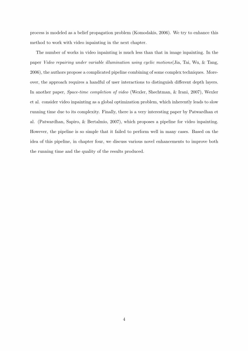
In this section, we briefly discuss our proposed pipeline at a high-level viewpoint. Funda-

mentally, given a damaged videoclip, our system performs a sequence of pre-processing steps,

followed by a sequence of processing steps, as depicted in figure 4.1.

In the pre-processing steps, the following tasks are executed

• Firstly, we detect the optical flows for the pixels in all frames

• Utilize the optical flows detected, we figure out the camera motion. Although we can

detect the zooming motion quite accurately, in our method, we only consider static and

13

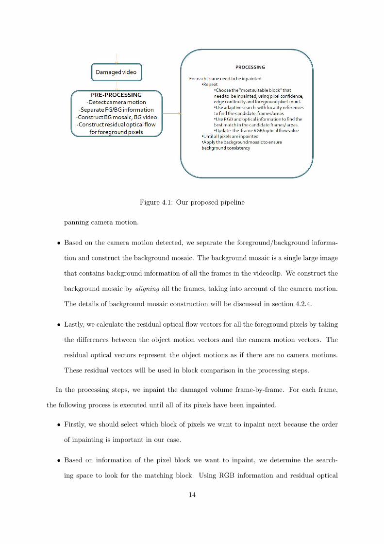
Figure 4.1: Our proposed pipeline

panning camera motion.

• Based on the camera motion detected, we separate the foreground/background informa-

tion and construct the background mosaic. The background mosaic is a single large image

that contains background information of all the frames in the videoclip. We construct the

background mosaic by aligning all the frames, taking into account of the camera motion.

The details of background mosaic construction will be discussed in section 4.2.4.

• Lastly, we calculate the residual optical flow vectors for all the foreground pixels by taking

the differences between the object motion vectors and the camera motion vectors. The

residual optical vectors represent the object motions as if there are no camera motions.

These residual vectors will be used in block comparison in the processing steps.

In the processing steps, we inpaint the damaged volume frame-by-frame. For each frame,

the following process is executed until all of its pixels have been inpainted.

• Firstly, we should select which block of pixels we want to inpaint next because the order

of inpainting is important in our case.

• Based on information of the pixel block we want to inpaint, we determine the search-

ing space to look for the matching block. Using RGB information and residual optical

14

information, we can retrieve the best match.

• Using the best match, we inpaint the block, and update the foreground/background in-

formation and the optical information.

After all pixels in a frame has been inpainted, we replace the background pixels in the in-

painted area of this frame by the corresponding pixels in the background mosaic. This additional

step will ensure the consistencies of the background across all frames.

4.2 Pre-processing steps

In the pre-processing process, we make use of optical flow vectors to detect the camera mo-

tion. Based on the camera motion vectors, we separate the foreground/background information

and construct the background mosaic. The below sections describe each component in the

process.

4.2.1 Optical flow

Optical flow at a pixel represent the flow of this pixel from the current frame to the next

frame. In Figure 4.2, most of the optical vectors point to the up-left direction, representing the

camera motion panning down-right. Optical flow detection may suffer from aperture effects, in

which the optical vectors are calculated incorrectly, as the reader can observe in the area under

the front leg of the person in Figure 4.2.

To calculate the optical flow of a point in a frame, we make use of OpenCV function call,

as demonstrated in the tutorial by Stavens (Stavens, 2005).

4.2.2 Camera motion detection

Given the optical flows of the pixels detected in the first step, we propose a method to

approximate the camera motion. In this method, we only consider the case where the camera

15

Figure 4.2: Optical flows

motion is static or panning (i.e. zooming operation is not allowed). The reason is that in the

next step, we need to construct the background mosaic, which is incompatible with the zooming

operation.

In Figure 4.3, some camera motion operations are depicted. We observe that for each kind

camera motion, the optical vectors have their distinctive characteristics.

• For static camera motion and moving object, most optical vector magnitudes are near

zero, but some are bigger, representing the object motion.

• For camera panning motion, most of the optical vectors point to the same direction, but

some may point to other directions, representing the object motion.

Both of the observations above make use of the assumption that the foreground is relatively

small compared to the background.

Static camera motion

For static camera motion, most of the optical flows are zero, representing background pixels,

while the rest are much bigger than zero, representing the foreground object motion. Because of

some errors in calculating the optical flows, we set a small threshold to distinguish foreground

16

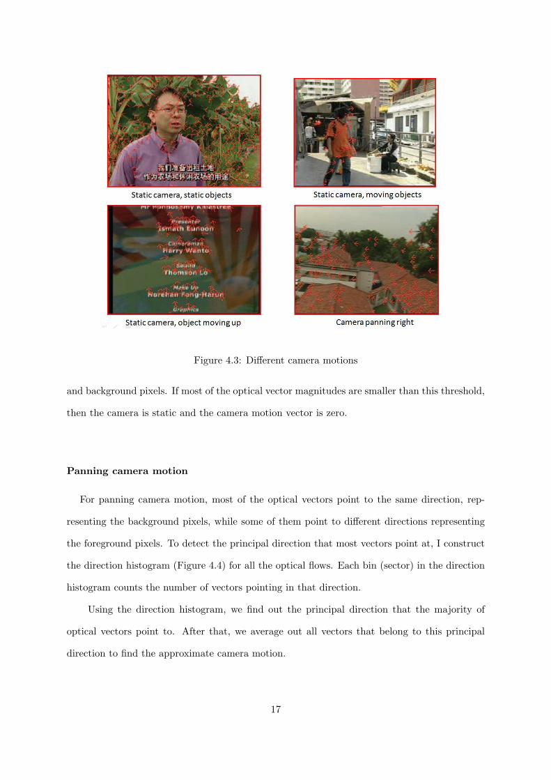
Figure 4.3: Different camera motions

and background pixels. If most of the optical vector magnitudes are smaller than this threshold,

then the camera is static and the camera motion vector is zero.

Panning camera motion

For panning camera motion, most of the optical vectors point to the same direction, rep-

resenting the background pixels, while some of them point to different directions representing

the foreground pixels. To detect the principal direction that most vectors point at, I construct

the direction histogram (Figure 4.4) for all the optical flows. Each bin (sector) in the direction

histogram counts the number of vectors pointing in that direction.

Using the direction histogram, we find out the principal direction that the majority of

optical vectors point to. After that, we average out all vectors that belong to this principal

direction to find the approximate camera motion.

17

Figure 4.4: Direction histogram

4.2.3 Foreground-Background separation

Applying the optical flow vectors and the camera motion detected in the first step, we now

have a tool to separate the foreground from the background. In this section, we discuss two

methods for separation. The first method is intuitive because it makes use of the optical flows

directly. The second method uses the idea of aligning two consecutive frames according to the

camera motion. We show that that both methods suffer from some limitations, leading to the

introduction of our novel method in section 4.2.5.

First approach

In this approach, we base on the observation that the background pixels often move together

with the camera motion, while the foreground pixels move differently from the camera motion.

Therefore, depending on the camera motion, we consider the optical flow at each pixel to classify

it as a foreground pixel or a background pixel.

• For static camera motion, we expect the optical vectors of background pixels are near

zero, while those of foreground pixels are much larger. Hence, optical magnitude is the

18

factor of classification in this case.

• For panning camera motion, a pixel belongs to the background if and only if its optical

vector agrees with the camera motion, both in magnitude and direction, which can be

decided by the following conditions

cameraV ector • opticalV ector‖cameraV ector‖ × ‖opticalV ector‖

> threshold1 (4.1)

andabs(‖cameraV ector‖ − ‖opticalV ector‖)abs(‖cameraV ector‖+ ‖opticalV ector‖)

> threshold2 (4.2)

Equation 4.1 ensures the similarity in direction between opticalV ector and cameraV ector

while equation 4.2 ensures their similarity in magnitude. Although this approach is simple

and intuitive, it suffers from serious limitations. The first limitation is that there may be the

case when some foreground pixels have the same optical flows as the camera vector. Based on

equation 4.1 and 4.2, they will be classified as background pixels. The second limitation, which

is more serious, is that the method is directly affected by the errors in optical flow detection,

which are unrare to happen. Therefore we propose another method.

Second approach

In this approach, based on the camera motion, we try to align two consecutive frames in such

a way that their corresponding pixels are aligned together. Let f1 and f2 be the two consecutive

frames in consideration, then the pixel at position (x,y) in frame f1 belongs to the background

if and only if

|f1b(x, y)− f2b(x+ dx, y + dy)| < diff threshold (4.3)

where (dx, dy) represents the camera motion from frame f1 to frame f2, as depicted in Fig-

ure 4.5 and fib(x, y) represents a block centered at (x,y) in frame fi. We make use of block

comparison because it is a much more accurate measurement than point comparison. Although

this method performs quite well with slow foreground movement, it produces errors when the

foreground moves fast enough. We call it the bi-directional effect, in which some background

pixels are classified as foreground pixels, and vice-versa.

19

Figure 4.5: Frame shift

Figure 4.6: Bi-directional effect

In Figure 4.6, f1 and f2 are two consecutive frames through which the camera motion is

static. The static background and moving foreground are denoted with bg and fg in the two

frames. The bottom image in Figure 4.6 describes what happens when we align the two frames

together: there are many foreground pixels which are classified as background, because of the

color differences, and vice-versa. The faster the foreground objects move, the more severe the

bi-directional effect becomes. This is a serious limitation which makes this method inapplicable

in practice.

Because of the intense disadvantages of the first two approaches, we want to find a more ro-

bust and effective way to separate the foreground and background information. A novel method

20

Figure 4.7: Background mosaic construction

is proposed, which utilizes the background mosaic. Hence, we will revisit this problem again

after discussing the construction of the background mosaic.

4.2.4 Background mosaic construction

Using the camera motions detected in the previous steps, we organize all the frames in such a

way that their background pixels are aligned together. We average out the aligned pixels to get

the value of the corresponding pixel in the result image, which is called the background mosaic.

Figure 4.7 shows the construction of a background mosaic, which fundamentally captures the

background information in all frames.

In the case of static camera motion or slow camera motion, the background mosaic may

have holes inside. These artifacts represent the fact that there exists a frame whose background

information cannot be filled in using other frames’ background information. In this situation,

we make use of image inpainting techniques to fill in the holes in the background mosaic.

21

4.2.5 Foreground-Background separation revisit

Given the background mosaic, we have a new way to separate the foreground and background

information. Based on the camera motion vectors that we have calculated in previous steps, the

projected location of a frame inside the background mosaic can be determined easily. If a frame

is projected onto the background mosaic, its background pixels align with the background

mosaic pixels, while its foreground pixels are different from the corresponding pixels in the

background mosaic. Therefore, the background mosaic can be used as an effective tool for

foreground-background separation.

In particular, the pixel (x,y) in frame f belongs to the background if and only if

|fb(x, y)−mosaicb(x+ cx, y + cy)| < threshold (4.4)

In Equation 4.4

• fb(x, y) represents the block centered at position (x,y) in frame f.

• mosaicb(x, y) represents the block centered at position (x,y) in the background mosaic.

• (cx,cy) represents the location of frame f inside the background mosaic.

• threshold is a value set by the user.

Although this process is much more robust and accurate than the two other approaches we

discussed in section 4.2.3, there is still a problem that we have not brought up. On the one hand,

the construction of the background mosaic mentioned in section 4.2.4 requires the background

information to be filtered out from the foreground information before we can perform averaging,

whichs mean the separation process must be performed before the mosaic construction process.

On the other hand, in the proposed method above, the mosaic should come before the separation

process. This leads to a chicken-and-egg problem that we have to solve.

For resolving this chicken-and-egg issue, on the one hand, we observe that the construction

of background mosaic does not need the complete background information in all frames. The

reason is that a pixel in the mosaic is the average of all corresponding pixels across the videoclip;

therefore, if we cannot get the background information of a pixel from a particular frame, we

22

Figure 4.8: Foreground Background Separation: Preliminary step

may still manage to retrieve it from other frames. Therefore, we can sustain many false negatives

(i.e. background pixels being classified as foreground pixels) without decreasing the quality of

the background mosaic. On the other hand, we notice that false positives (i.e. foreground pixels

being classified as background pixels) may cause direct inaccuracy to the background mosaic.

As a result, we conclude that false negatives are much less severe than false positives, leading

to the strategy that we should decrease the number of false positives with the cost of increasing

the number of false negatives.

Based on the above observation, we suggest a three-step foreground-background separation

process using the background mosaic.

• Preliminary step: In this step, we use the first approach described in section 4.2.3

to perform basic separation. To reduce the number of false positives, we compute the

bounding boxes of the foreground pixels and consider all the pixels inside the bounding

boxes as foreground pixels, and the others as background pixels. The result of this step

can be visualized in Figure 4.8.

• Mosaic construction step Using the background information determined in the prelim-

inary step, we apply the method described in section 4.2.4 to construct the background

mosaic .

23

• Separation step Having the background mosaic, we can now employ the method dis-

cussed at the beginning of this section to separate the foreground and the background

information. This three-step process is proved to outperform the two approaches dis-

cussed in section 4.2.3 in both quality aspect and robustness aspect.

4.2.6 Products of the pre-processing steps

After performing the pre-processing steps, we acquire the following products to use in the

processing steps

• Background mosaic

• Foreground/background information for all the frames

• Camera motions for all the frames which can be used to locate the position of each frame

inside the background mosaic

• Residual optical vectors for all the foreground pixels in all frames

4.3 Processing steps

In this section, we describe our method to perform video inpainting. Firstly, we discuss the

issues that need to be taken into consideration and then we discourse our general matching

method. After that, we come to the main part: space reduction techniques. Lastly, we talk

about the order of inpainting.

4.3.1 Difficulties

Although the intermediate products generated from the previous steps will significantly re-

duce the difficulties in this process, there are a number of issues that we need to consider

• The video inpainting process should maintain both the spatial and the temporal consis-

tencies. Therefore, we must make sure that the final video should not flicker when we

move from frame to frame. We can ensure this property using the background mosaic and

the optical flow information, which will be described later.

24

Figure 4.9: General block matching

• Provided that the number of pixels need to be inpainted is quite numerous, it would be

inapplicable if for every pixel, we need to search in all frames to find the best match.

Hence, reducing the searching space is crucial for the success of the inpainting process.

• The order of inpainting is also very important. In principle, we should inpaint the pixels

with high confidence values first, and then move to less confident pixels. This order will

generate a better result in most cases.

The issues that we address above will be resolved in the subsequent sections.

4.3.2 General block matching method

This section provides the reader with the fundamentals of the matching method that we

employ. In our algorithm, after deciding which pixel we want to inpaint next, we define a block

centered at that pixel. The block will be used as the template for matching. After retrieving

the best match (maybe from the same frame or from a different frame), we use the information

of that best match to fill the unknown pixels in the template. This method produces much more

consistent results than pixel-by-pixel matching.

A subtle improvement of this matching method is that instead of trying to match all the

pixels inside a block, we only need to match the confident pixels in the template. A confident

25

pixel is defined as a pixel which has been inpainted or does not need to be inpainted. This idea

is quite intuitive, because it will be unreasonable if we try to find a match with some unknown

pixel values. Figure 4.9 describes the matching process, during which a mask is constructed.

The black area in the mask is the only area that we need to consider. Using the mask, we only

need to compare the confident area in the template with the corresponding area in the matching

block. The Euclidean distance between the two areas can be used as the block difference.

4.3.3 Searching space reduction

This section is the most crucial part of the processing pipeline. It decides whether the method

is feasible for practical use or not. In this section, we propose several methods to reduce

the searching space: the first method makes use of the background mosaic to quickly inpaint

the background; the second method employs block sampling to increase the searching speed

to several times; finally, the last method applies the idea of locality references in caching for

inpainting the foreground.

Application of the background mosaic

Given the fact that the background mosaic comprises of the background information in all

frames, whenever we need to search for background information, we can directly apply the

searching process in the mosaic instead of having to go through all the frames in the videoclip.

In Figure 4.10, the upper figure represents a frame that we want to perform searching, while

the lower figure represents the background mosaic. We observe that all background blocks in

the frame have been captured in the background mosaic already. Therefore, the searching space

for each template is reduced to the background mosaic and the foreground areas in all frames.

One improvement over the application of the background mosaic is that instead of searching

the whole background mosaic for background information, we can directly retrieve the correct

block using the location of the frame (which we want to inpaint) inside the background mosaic.

Let us consider an example where we want to inpaint the block located at position (x,y) in frame

f . Assume that the location of f inside the background mosaic is (cx, cy), which can easily be

26

Figure 4.10: Background mosaic captures all background information

calculated using the camera motion information then we can retrieve the block centered at (x

+ cx, y + cy) in the background mosaic as the best match for the background. This idea is

show in Figure 4.11.

With the above discussion, we can perform background matching in constant time. However,

the foreground matching process is still time-consuming, as we need to go through all frames.

Therefore, it would be very helpful if we know whether it is necessary to search for foreground

information or not. If we know that the best match for a template certainly comes from the

background, then we can directly retrieve the best match in the background mosaic, without

considering the foreground information.

Our idea for resolving this problem is that if all surrounding confident pixels come from the

background, then it is very likely that the surrounded pixels that we need to inpaint come from

the background as well, because there are no foreground consistency that we need to maintain.

To approximate this idea, we employ the condition that if all confident pixels in the template

come from the background, we just retrieve the matching block directly from the background

mosaic, without considering the foreground information. However, for this condition to apply

correctly, we must be careful not to delete the foreground seeds. This means the order of

27

Figure 4.11: Direct block retrieval using background mosaic

inpainting is also very important.

Block sampling

In the previous section, we conclude that the background mosaic makes the background

inpainting task very effective and efficient, because it helps inpaint a block of background in

constant time. Therefore, our bottleneck is now lying on the foreground inpainting process. For

the foreground inpainting, we apply two methods to cut down the searching space. The first

method is block sampling, which brings the searching space down several times. The second

method makes use of locality references in caching, which potentionally minifies the searching

space to hundreds of times smaller. This section covers the block sampling, and the next section

discusses locality references.

The idea of block sampling is that for foreground template (i.e. templates which contains at

least one foreground pixels), instead of searching all foreground blocks in the videoclip, we can

apply block sampling to reduce the number of candidates. From our experiment, we suggest

that the sampling size should not be more than 4 × 4, because large sampling size will cause

28

Figure 4.12: Block Sampling

serious artifacts in the result video.

In Figure 4.12, the size of block sampling is 2 × 2, which means for every 2 × 2 block in

a frame (at the dot position), we perform a matching with the template. This will effectively

reduce the searching space by 4 times.

Making use of locality references

For further enhancement of the foreground inpainting process, we introduce a new method

using the idea from locality references in caching. The idea is that if we know all neighboring

pixels of the pixel (x, y) in frame f come from a particular area, then there is a great probability

that the pixel (x, y) also comes from somewhere near that area (in both the spatial and the

temporal domain).

For applying the idea into our implementation, we set a threshold, which will determine

the hit or miss of the locality references. For an inpainted pixel P , which is the center of the

template T , we only search in the areas near the locations where its neighbors was found.

• If the minimum difference between the blocks with T is smaller than threshold, we define

this as a hit. In this case, we just use the best match to inpaint P .

• If the minimum difference between the blocks with T is bigger than threshold, we define

this as a miss. This case means that the searching area we are using is not good enough.

29

Therefore, we need to expand the searching area for a better match.

4.3.4 Consistency assurance using background mosaic

Besides the function of significantly reducing the searching space for background blocks to

constant time, the background mosaic can also be used to maintain the background consistencies

through all the inpainted frames. For that purpose, we apply the background mosaic to a frame

after that frame has been fully inpainted. The pixels in the background mosaic are used to

replace the corresponding inpainted background pixels in the frame. By doing this, we can

make sure that there are no sudden change in the background across all frames.

4.3.5 Order of inpainting

As we discussed before, the order of inpainting is also a crucial part in the inpainting process.

In many cases, a suitable order of inpainting can dramatically improve the quality of the result

videoclip. Moreover, in section 4.3.3, we also mentioned that the order of inpainting should not

delete the foreground seed. Therefore, we should be very careful when selecting the next block

to inpaint.

In general, the block that we select to inpaint next should have the following characteristics.

• The block should have many confident pixels. The reason is that with many confident

pixels, the number of uncertainties will be reduced and many false matches can be elim-

inated. This confident value may be represented as the ratio of the number of confident

pixels over the block area.

• The block should also have some foreground pixels. The reason is that we are using the

background mosaic for background inpainting and we do not want to accidentally delete

some foreground seeds, as discussed in section 4.3.3. Therefore the foreground blocks

should have much higher priority than the background blocks.

• The block should contain some edges, because the edges will make the matching process

more accurate as the aperture effects can be cut down. We use the the Canny function in

30

OpenCV to detect the edges. If a block contains some edges, we assign it a higher priority

than other blocks.

• We also want to inpaint the blocks near the boundary of the inpainted area instead of the

internal blocks. This preference is because the more distant a block is from the boundary,

the more errors it will receive from the propagation of other inpainted blocks. Therefore,

a boundary block should have a higher confident value than an internal block.

Using a suitable combination of the above four heuristics, we can decide the block that needs

to be inpainted next.

4.3.6 Block comparison enhancement

The last enhancement that we want to discuss about is the method to compare a template

with a particular block. In section 4.3.2, we mentioned that for comparing two blocks, we use

the Euclidean distance between the two corresponding confident areas. However, this method

does not take into account of the available foreground/background information, hence may lead

to an undesirable result. In particular, this method assumes that whenever the foregrounds

match each other, the backgrounds also match, which is quite unlikely in reality. Therefore,

we should have a different mechanism for comparing two blocks. Because the purpose of block

matching is to inpaint the foreground, we should give a higher weight to the foreground pixels

when calculating the block distance. In practice, if the background is non-uniform, we may not

want to consider the background pixels at all in block matching. The idea is represented in

Figure 4.13.

Figure 4.13 is different from Figure 4.9 in the aspect that it only considers the foreground

area instead of the whole confident area. However, there is one subtle issue that we should

resolve. Let use consider Figure 4.14, where there are two candidate blocks to be matched with

the template block at the top. Clearly, the left figure is a better match than the right figure.

However, if we do not consider the background pixels, the two candidates will have the

same distance to the template, which is not exactly what we want. Hence, we want to apply

some penalties in the case when a block pixel belongs to the foreground while its corresponding

31

Figure 4.13: Block Comparison Enhancement

Figure 4.14: A subtle issue in block comparison

32

template pixel belongs to the background and vice-versa. This enhancement will make the left

figure more similar to the template than the right figure.

The Euclidean distance that we apply to find the block difference is actually a linear com-

bination of two separate Euclidean distances: RGB distance and optical distance. The RGB

distance accounts for the difference in color while the optical distance accounts for the difference

in motion. A linear combination between the two distances will ensure the spatial continuity as

well as the motion continuity. Equation 4.5 represents the formular for block distance, in which

α represents the weight of RGBDistance.

BlockDistance = α×RGBDistance+ (1− α)×OpticalDistance (4.5)

4.4 Result

Applying the above enhancements makes our method applicable to practical problems. The

space reduction techniques enable our method to run in a reasonable amount of time, while

other heuristics assure the quality of final videoclip. Figure 4.15 shows some of the frames that

have been inpainted using our method.

33

Figure 4.15: Result

34

Chapter 5

Discussion

5.1 Our contribution

Although our work makes use of the idea proposed in the paper by Patwardhan (Patwardhan

et al., 2007), our method is significantly different from theirs because we have employed plenty

of enhancements:

• In the paper (Patwardhan et al., 2007), the authors use a very simple estimation to

determine the camera motion (they just consider the median of all optical flow vectors as

the camera vector). This is not robust because the method does not take into account the

vector directions, and in some cases, it may fail to detect the right direction of the camera

movement. Our method uses the direction histogram to filter out the unsatisfiable vectors

before calculating the real camera motion; therefore it will be more robust.

• The authors also use a very simple technique to separate the foreground/background

informations. They consider a pixel to be in the background if and only if the optical

vector of this pixel is similar to the camera motion vector. This method bases on the

assumption that the optical vectors of all pixels are all determined accurately. However,

in reality, the optical flow detection is very vulnerable to aperture effect, which causes

direct errors to the separation process. In our case, however, we construct the background

mosaic first, and use it to separate the foreground from the background. The construction

35

of the background mosaic is tolerant of the errors in optical flow detection; therefore, our

method can sustain optical flow errors.

• When performing block matching, Patwardhan et al. use 5D vectors (3 for RGB values

and 2 for optical values) to calculate block distance, without taking into account the scale

of the each dimension. This may lead to the case when the RGB values over-dominate

the optical values (which happens most of the time), which will cause deficiencies in the

temporal importance. In our case, we also do normalization of the RGB values and the

optical values, and take the linear combination of the two distances. Therefore it produces

a more balanced block matching mechanism.

• Our main contribution in this project lies in the reduction of the searching space for can-

didate matching blocks. Locality references, if applied correctly, can reduce the searching

space by hundreds of times, while increase the temporal and spatial consistencies, because

neighboring blocks should come from the same area. In addition, block sampling will fur-

ther reduces the number of candidates. Moreover, using direct retrieval in the background

mosaic (without considering the foreground frames) will almost reduce the background

inpainting process to constant time. Combining these methods together enables the video

inpainting process to run in a reasonable amount of time and still produce acceptable and

consistent results.

5.2 Limitation

Although our method employs many novel heuristics to reduce the searching space, it still

has some limitations, which give spaces for further improvements.

• Our method cannot solve the case where the the camera operation is zooming. When this

case happens, the background mosaic cannot be constructed. Moreover, with zooming,

the method of copying blocks from one frame to another will not be accurate and it may

cause artifacts.

36

• Right now, our implementation can only deal with static rectangular inpainting areas.

With dynamic or arbitrary-shaped inpainting areas, although the idea of our method

is the same, we need to make some modifications in our implementation. This will be

considered as a future enhancement for this project.

• Our second approach is a combination of many heuristics. Unlike the first approach,

which makes use of BP, distance transform and PCA, the second approach does not

have a strong theoretical background. Moreover, having too many heuristics will cause

difficulties in choosing the best combination of heuristics to apply. This is also considered

as a limitation of our method.

37

Chapter 6

Conclusion

Through out the project, we have introduced our novel methods to inpaint a damaged video-

clip. Although the methods still have some limitations and the results still contain some arti-

facts, we have studied a lot from this project. During the first approach, we studied how to

extend the image inpainting problem to the video inpainting problem using belief propagation.

The introduction of Distance Transform and PCA to video inpainting for reducing the number

of dimensions is original and it may give ways for future research in this field. During the

second approach, we need to attempt many methods in order to propose a nice and elegant way

to separate the foreground and background informations. Moreover, we also need to study the

problem very carefully to come up with a variety of heuristics to reduce the searching space.

The knowledges we learnt through out the whole project will benefit us in our further research

in computer vision.

38

References

Bertalmio, M., Sapiro, G., Caselles, V., & Ballester, C. (2000). Image inpainting. SIGGraph-2000 (pp. 417–424), 2000.

Efros, A., & Leung, T. (1999). Texture synthesis by non-parametric sampling (pp. 1033–1038),1999.

Felzenszwalb, P., & Huttenlocher, D. (2004). Distance transforms of sampled functions, 2004.

Fidaner, I. (2008). A survey on variational image inpainting, texture synthesis and imagecompletion (pp. 1–13), 2008.

Jia, J., Tai, Y., Wu, T., & Tang, C. (2006). Video repairing under variable illumination usingcyclic motions. 28 (5), May, 2006, 832–839.

Komodakis, N. (2006). Image completion using global optimization (pp. I: 442–452), 2006.

Osher, S., Sapiro, G., Vese, L., & Bertalmio, M. (2003). Simultaneous structure and textureimage inpainting (pp. II: 707–712), 2003.

Patwardhan, K., Sapiro, G., & Bertalmio, M. (2007). Video inpainting under constrainedcamera motion. 16 (2), February, 2007, 545–553.

Smith, L. (2002). A tutorial on principle components analysis, 2002.

Stavens, D. (2005). The opencv library: Computing optical flow. , 2005.

Szeliski, R., Zabih, R., Scharstein, D., Veksler, O., Kolmogorov, V., Agarwala, A., Tappen, M.,& Rother, C. (2008). A comparative study of energy minimization methods for markovrandom fields with smoothness-based priors. 30 (6), June, 2008, 1068–1080.

Wexler, Y., Shechtman, E., & Irani, M. (2007). Space-time completion of video. 29 (3), March,2007, 463–476.

Yedidia, J., Freeman, W., & Weiss, Y. (2002). Understanding belief propagation and itsgeneralizations, 2002.

39