
Victoria University Employment Forecasts - … University Employment Forecasts ... As a generation...
36
Victoria University Employment Forecasts 2017 edition CoPS Working Paper No. G-277, October 2017 The Centre of Policy Studies (CoPS), incorporating the IMPACT project, is a research centre at Victoria University devoted to quantitative analysis of issues relevant to economic policy. Address: Centre of Policy Studies, Victoria University, PO Box 14428, Melbourne, Victoria, 8001 home page: www.vu.edu.au/CoPS/ email: [email protected] Telephone +61 3 9919 1877 Janine Dixon Centre of Policy Studies, Victoria University ISSN 1 031 9034 ISBN 978-1-921654-85-5
Transcript of Victoria University Employment Forecasts - … University Employment Forecasts ... As a generation...

Victoria University Employment Forecasts
2017 edition
CoPS Working Paper No. G-277, October 2017
The Centre of Policy Studies (CoPS), incorporating the IMPACT project, is a research centre at Victoria University devoted to quantitative analysis of issues relevant to economic policy. Address: Centre of Policy Studies, Victoria University, PO Box 14428, Melbourne, Victoria, 8001 home page: www.vu.edu.au/CoPS/ email: [email protected] Telephone +61 3 9919 1877
Janine Dixon
Centre of Policy Studies, Victoria University
ISSN 1 031 9034 ISBN 978-1-921654-85-5


1
Victoria University Employment Forecasts 2017 edition
Janine Dixon, Centre of Policy Studies, October 2017
This report was written to accompany the 2017 Victoria University Employment Forecasts, a
comprehensive and detailed set of medium-term forecasts of employment in Australia commissioned
by most of Australia’s state and territory governments. The forecasts were prepared at Victoria
University’s Centre of Policy Studies by Dr Janine Dixon, with valuable assistance from Dr Longfeng Ye.
The Centre of Policy Studies’ employment forecasting project, now in its 24th year, was led by Dr Tony
Meagher until his retirement in 2013, and the project still benefits greatly from his advice and expertise.
The author is grateful to Adjunct Associate Professor Chandra Shah for his feedback on this report.
Parts of this paper are reproduced from an unpublished 2016 information paper by the same author.
Centre of Policy Studies, Victoria University
www.vu.edu.au/centre-of-policy-studies-cops www.copsmodels.com

2
Abstract
Over the next eight years, employment in Australia will grow to almost 14 million jobs, a net increase
of some 1.6 million jobs. In which industries and regions will these jobs be? What occupations will
the workers perform? The labour market in Australia is constantly changing. It is unlikely that these
questions will have the same answers in 2025 that they have today.
The Victoria University Employment Forecasting (VUEF) project attempts to address these questions,
in the context of a macroeconomic model that has the capacity to incorporate detailed structural and
demographic change. As a generation of baby-boomers retires and a new generation – many with
degree-level qualifications in management and commerce, society and culture, health and other fields
– enters the workforce, the service industries will continue to dominate. The modelling finds that just
three industry divisions – health care and social assistance, professional services, and education and
training – will account for more than half of employment growth over the next eight years.
Accordingly, employment in the professional occupations will continue to grow strongly, adding
almost 600,000 jobs to employ 3.4 million people, or a quarter of the workforce, by 2025.
A gradual reversal of some of the adverse conditions affecting employment in the manufacturing and
agricultural sectors will see a return to positive, albeit modest, growth rates in these sectors.
High urban population growth forecasts and the dominance of growth in the service industries mean
that more than 75 per cent of employment growth, or a net increase of 1.2 million jobs, will be in the
capital cities. Melbourne and Sydney will account for just over half of the forecast growth in national
employment.
Full or partial subscriptions to the 2017 edition of the detailed VUEF database are now available from
the Centre of Policy Studies at Victoria University.
JEL: J21, J23, J24, J11
Key words: employment, forecast, occupation, industry, skill, Australia, regions, CGE model

3
Contents
1 Background and introduction ......................................................................................................... 7
2 The model ....................................................................................................................................... 8
2.1 Overview of VUEF ................................................................................................................... 8
2.2 The VU historical and forecast CGE simulations ................................................................... 11
2.2.1 Population, labour force and aggregate employment .................................................. 11
2.2.2 Macroeconomic context ............................................................................................... 14
2.2.3 Structural change estimates ......................................................................................... 16
2.2.4 Industry expert forecasts .............................................................................................. 19
2.3 Qualification supply estimates and cohort model ................................................................ 21
2.3.1 Historical data ............................................................................................................... 21
2.3.2 Skill forecasts ................................................................................................................ 22
2.4 Regional forecasts ................................................................................................................. 24
3 The employment forecasts ........................................................................................................... 25
3.1 Industries .............................................................................................................................. 25
3.1.1 Overview ....................................................................................................................... 25
3.1.2 Strong growth industries............................................................................................... 26
3.1.3 Slow growth industries ................................................................................................. 26
3.1.4 Improving industries ..................................................................................................... 27
3.2 Occupations .......................................................................................................................... 29
3.3 Regions .................................................................................................................................. 30
4 Conclusions ................................................................................................................................... 32
5 References .................................................................................................................................... 33
4
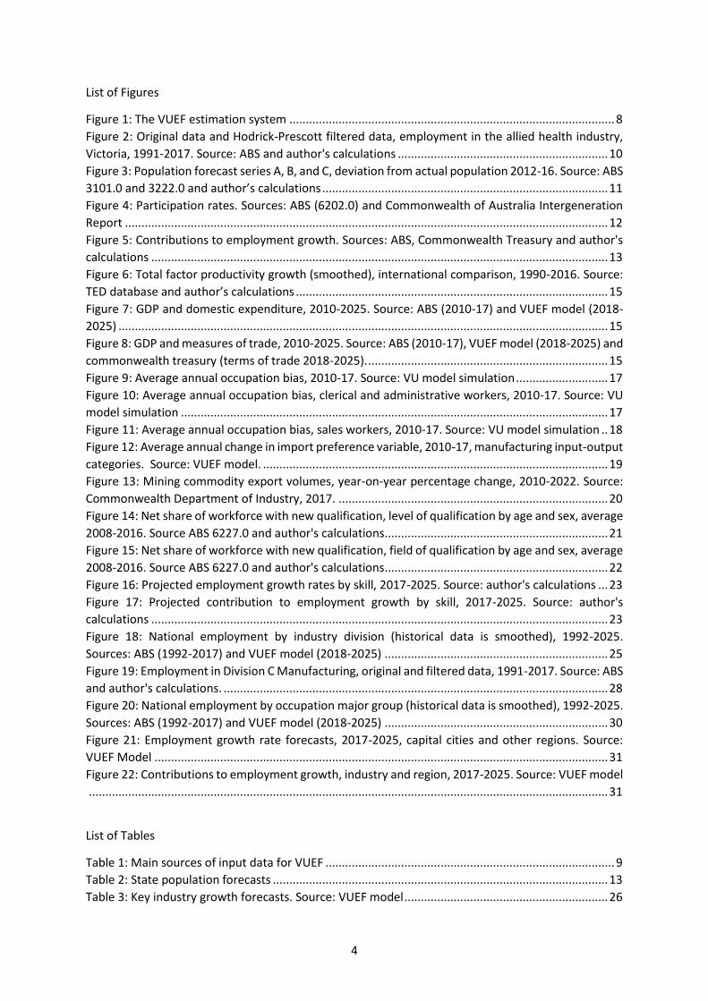
List of Figures
Figure 1: The VUEF estimation system ................................................................................................... 8
Figure 2: Original data and Hodrick-Prescott filtered data, employment in the allied health industry,
Victoria, 1991-2017. Source: ABS and author's calculations ................................................................ 10
Figure 3: Population forecast series A, B, and C, deviation from actual population 2012-16. Source: ABS
3101.0 and 3222.0 and author’s calculations ....................................................................................... 11
Figure 4: Participation rates. Sources: ABS (6202.0) and Commonwealth of Australia Intergeneration
Report ................................................................................................................................................... 12
Figure 5: Contributions to employment growth. Sources: ABS, Commonwealth Treasury and author's
calculations ........................................................................................................................................... 13
Figure 6: Total factor productivity growth (smoothed), international comparison, 1990-2016. Source:
TED database and author’s calculations ............................................................................................... 15
Figure 7: GDP and domestic expenditure, 2010-2025. Source: ABS (2010-17) and VUEF model (2018-
2025) ..................................................................................................................................................... 15
Figure 8: GDP and measures of trade, 2010-2025. Source: ABS (2010-17), VUEF model (2018-2025) and
commonwealth treasury (terms of trade 2018-2025). ......................................................................... 15
Figure 9: Average annual occupation bias, 2010-17. Source: VU model simulation ............................ 17
Figure 10: Average annual occupation bias, clerical and administrative workers, 2010-17. Source: VU
model simulation .................................................................................................................................. 17
Figure 11: Average annual occupation bias, sales workers, 2010-17. Source: VU model simulation .. 18
Figure 12: Average annual change in import preference variable, 2010-17, manufacturing input-output
categories. Source: VUEF model. ......................................................................................................... 19
Figure 13: Mining commodity export volumes, year-on-year percentage change, 2010-2022. Source:
Commonwealth Department of Industry, 2017. .................................................................................. 20
Figure 14: Net share of workforce with new qualification, level of qualification by age and sex, average
2008-2016. Source ABS 6227.0 and author's calculations .................................................................... 21
Figure 15: Net share of workforce with new qualification, field of qualification by age and sex, average
2008-2016. Source ABS 6227.0 and author's calculations .................................................................... 22
Figure 16: Projected employment growth rates by skill, 2017-2025. Source: author's calculations ... 23
Figure 17: Projected contribution to employment growth by skill, 2017-2025. Source: author's
calculations ........................................................................................................................................... 23
Figure 18: National employment by industry division (historical data is smoothed), 1992-2025.
Sources: ABS (1992-2017) and VUEF model (2018-2025) .................................................................... 25
Figure 19: Employment in Division C Manufacturing, original and filtered data, 1991-2017. Source: ABS
and author's calculations. ..................................................................................................................... 28
Figure 20: National employment by occupation major group (historical data is smoothed), 1992-2025.
Sources: ABS (1992-2017) and VUEF model (2018-2025) .................................................................... 30
Figure 21: Employment growth rate forecasts, 2017-2025, capital cities and other regions. Source:
VUEF Model .......................................................................................................................................... 31
Figure 22: Contributions to employment growth, industry and region, 2017-2025. Source: VUEF model
.............................................................................................................................................................. 31
List of Tables
Table 1: Main sources of input data for VUEF ........................................................................................ 9
Table 2: State population forecasts ...................................................................................................... 13
Table 3: Key industry growth forecasts. Source: VUEF model .............................................................. 26

5
Commonly used terms
“2017” etc Refers to financial year ending June 2017 unless otherwise specified
ANZSCO Australian and New Zealand Standard Classification of Occupations. Number in brackets refers to level of classification where relevant (1 = major group, 2 = sub-major group, 3 = minor group; 4 = unit group)
ANZSIC Australian and New Zealand Standard Industrial Classification (2006). Number in brackets refers to level of classification where relevant (1 = division, 2 = sub-division, 3 = group; 4 = class)
ASCED Australian Standard Classification of Education
CGE Computable General Equilibrium
GDP Gross Domestic Product
Labour force Persons working or actively seeing work, also referred to as “workforce”
NDIS National Disability Insurance Scheme
ORES ORANI Regional Extension System
Participation rate
The proportion of the working age population working or actively seeking work
Skill Unless otherwise indicated, “skill” refers to the highest post-school qualification held by an individual or cohort
Terms of trade Ratio of export price index to import price index
Unemployment rate
The proportion of the labour force that is unemployed, that is, without work in the reference week, actively looking for work in the previous four weeks, and available to start work in the reference week
VU Model Victoria University CGE Model, a MONASH-style model of the Australian economy (Dixon and Rimmer 2002)
VUEF Victoria University Employment Forecasts
VUEF Model Suite of programs and data, including VU Model, used to estimate VUEF
Working age population
Population aged over 15. (Note that we assume no upper limit on working age)

6
Executive Summary
Over the next eight years, employment in Australia will grow by some 1.6 million jobs, to almost 14
million. In which industries and regions will these jobs be? What occupations will the workers
perform? The labour market in Australia is constantly changing. It is unlikely that these questions will
have the same answers in 2025 that they have today.
The Victoria University Employment Forecasting (VUEF) project attempts to address these questions,
in the context of a macroeconomic model that has the capacity to incorporate detailed structural and
demographic change. The model draws on a comprehensive range of inputs, including
macroeconomic and demographic data, labour market statistics, education statistics, commonwealth
and state economic and demographic forecasts, and expert industry forecasts.
The VUEF forecasts are very detailed, covering 214 industries, 358 occupations, 57 regions and several
other classifications. The full forecast database, commissioned by most of Australia’s state and
territory governments, is available on a subscription basis from the Centre of Policy Studies at Victoria
University. Partial subscriptions are also available.
The following are some key messages from the forecasts:
The workforce will be more educated. Every year, the workforce contains fewer people with no post
school qualifications. As a generation of baby-boomers retires, a new generation – many with degree-
level qualifications in management and commerce, society and culture, health and other fields – will
enter the workforce. The number of workers with degree-level qualifications is forecast to grow by 1
million by 2025. These workers will perform professional and managerial occupations, primarily in
the service industries.
Service industries and professional occupations will be dominant. Three industry divisions – health
care and social assistance, professional services, and education and training – will account for more
than half of employment growth over the next eight years. Accordingly, employment in the
professional occupations will continue to grow strongly, adding almost 600,000 jobs to employ 3.4
million people, or a quarter of the workforce, by 2025.
Growth in manufacturing and agriculture will recover. A gradual reversal of some of the adverse
conditions affecting employment in the manufacturing and agricultural sectors will see a return to
positive, albeit modest, growth rates in these sectors.
Urbanisation of employment will continue. The dominance of service industries and high urban
population growth forecasts mean that more than 75 per cent of employment growth, or 1.2 million
jobs, will be in the capital cities. Melbourne and Sydney will account for just over half of the forecast
growth in national employment.

7
1 Background and introduction Early versions of the CoPS employment forecasting methodology were documented by Meagher et al
(1996, 2000, 2011). In its early days, the employment forecasting project incorporated external
macroeconomic forecasts from various external agencies, including at times Syntec and Access
Economics. The model made efficient use of computing power, estimating highly disaggregated
forecasts of employment in a staged process, in which forecasts for occupations and qualifications
were based on forecasts of industry employment from a CGE model.
Advances in computing have meant that more aspects of the model are now run simultaneously.
Giesecke et al (2011, 2015) adopted an integrated approach in modelling the labour market of
Vietnam, in which forecasts of qualifications were input into the model. Qualification supply imposed
a restriction on occupation supply, and workers were assumed to choose an occupation based on the
relative wages of the occupations for which they were qualified.
The current VUEF qualification supply specification is similar to that of Giesecke et al. Qualification,
occupation and industry forecasts are now produced in the core CGE model, and not by auxiliary
programs such as the Labour Market Extensions used by Meagher et al (2000). This paper describes
the current form of the VUEF model, in the context of the 2017 version of the employment forecasts.
The paper begins by describing the model as a framework in which a large body of macroeconomic,
demographic, labour market and industry data is brought together in a single comprehensive
framework. Key inputs to and outputs from the model are described in subsequent sections.
Macroeconomic forecasts are described along with other inputs and assumptions to the model. Some
macroeconomic forecasts are adopted from external sources and others are derived within the model.
Although they are model outputs, the macroeconomic forecasts are described alongside other model
inputs because they are an integral part of the background to the detailed employment forecasts.
The 2017 forecasts are described in Section 3. The full set of forecasts is available electronically on a
subscription basis. The forecasts include the following seven key matrices of base year (2017) data
and forecasts for the period 2018-2025:
- Region x Industry x Occupation;
- Region x Occupation x Level of qualification;
- Region x Occupation x Field of qualification;
- Region x Level of qualification x Field of qualification;
- Region x Occupation x Demographic status;
- Region x Occupation x Hours worked; and
- Region x Demographic status x Hours worked.
The paper finishes with conclusions in Section 4.

8
2 The model
2.1 Overview of VUEF The VUEF model is in fact a family of models, centred on the VU CGE Model of the Australian economy
(closely related to the MONASH model, Dixon and Rimmer (2002)). The links between the VU CGE
model and various auxiliary programs are illustrated in Figure 1. As shown in Figure 1, the VUEF model
brings together a large body of demographic data, employment data, and macroeconomic data, as
well as forecasts from government and industry bodies, into a single set of detailed employment
forecasts for Australia and its regions. Some of the main data sources are listed in Table 1. This section
provides an overview of the VUEF model, and a discussion of the inputs and assumptions underlying
the model.
The VUEF system diagram (Figure 1) colour-codes the parts of the VUEF model, including the CGE
model runs and other calibration processes (pink), input data (blue), and intermediate data estimates
(yellow). In the centre of the diagram are two CGE simulation runs: an historical simulation (2010 to
2017) and a forecast simulation (2017 to 2025).
The purpose of the VU historical CGE simulation is twofold. Firstly, it facilitates the estimation of a
detailed, timely database that is consistent with the most recent observations of economic conditions.
These are described by macroeconomic aggregates including GDP or total employment, and also
incorporate detailed labour market statistics including employment by industry and occupation. The
database is also consistent with detailed but less recent data, such as input-output data or census
data. Secondly, the historical simulation is used to estimate changes in structural variables, such as
tastes and production technologies, following Dixon and Rimmer (2002). These structural estimates
also feed into the forecast process.
Figure 1: The VUEF estimation system

9
Table 1: Main sources of input data for VUEF
The VU forecast CGE simulation is the process in which forecast employment is estimated by industry
and occupation from 2018 to 2025. The forecast CGE simulation combines many sets of inputs:
estimates of structural change derived from the historical simulation, skill supply estimates derived
ABS SOURCES
Census of Population and Housing, 2011
Employment by: Industry (4) and occupation (4) Occupation (4) by demographic group Occupation (4) by hours worked Hours worked by demographic Occupation (4) by qualification level and field Demographic by region (LGA) Industry (4) by region (LGA)
Survey of Education and Work (6227.0)
Highest post-school qualification by level and age Highest post-school qualification by field and age.
Labour force detailed quarterly (6291.0.55.003)
Industry (3) by state by sex Occupation (4) by state by sex Occupation (1) by Industry (1) by sex Occupation (2) by age (10) by sex Occupation (1) by age (5) Occupation (1) by hours worked
National accounts (5206.0) GDP (real and nominal), consumption (public and private), investment (aggregate and dwellings), exports, imports, terms of trade, CPI
Labour force (6202.0) Aggregate employment, aggregate labour supply, unemployment rate, average hours worked per person
Balance of Payments and International Investment Position (5302.0)
Current account deficit
Wage price index (6345.0) Real wage Demographic Statistics (3101.0) Total population, working age population, aged population Population Projections 2012 base (3222.0)
Population forecasts by age and sex, Series C
Australian Industry (8155.0) Output per employee by Industry (1) Input-output tables (5209.0) International Trade in Goods and Services (5368.0)
Imports by commodity
NON-ABS SOURCES
State demographer forecasts Population by region and state State and federal budget forecasts Forecast GDP, unemployment rate, ratios of budget deficit
and government revenue to GDP, selected state government investment.
Inter-generation report Participation rates by age and sex (forecast), average hours worked per person (forecast).
Resources and Energy Quarterly Volume and value of commodity exports: Coal, Oil and Gas, Iron Ores, and Other Metal ores. Historical and forecast.
Tourism Research Australia forecasts Volume of tourism exports (forecast)

10
from the cohort model, various official macroeconomic and demographic projections, and forecasts
from industry bodies
Output from the CGE simulation is processed through several auxiliary programs. The national
calibration processes transform the estimates from the input-output industry classification used in the
CGE models to the more familiar ANZSIC industry classification. At this stage, the data is also
disaggregated by demographic group and average weekly hours worked.
The VU model is a national model, treating the Australia as an open, single region economy. To
generate regional estimates, a top-down regional simulation based on the ORES method (Dixon et al
1982) is used. Regional forecasts are calibrated to regional population estimates provided by the state
governments.
The national and regional estimates are passed through a final regional calibration process to generate
the VUEF Master database. This database includes seven key matrices of base year (2017) data and
forecasts for the period 2018-2025:
- Region x Industry x Occupation;
- Region x Occupation x Level of qualification;
- Region x Occupation x Field of qualification;
- Region x Level of qualification x Field of qualification;
- Region x Occupation x Demographic status;
- Region x Occupation x Hours worked; and
- Region x Demographic status x Hours worked.
For context, various tables of historical data dating back to 1991 are also included in the VUEF Master
database. Two versions of each series are provided: original and filtered. The series are smoothed
using the Hodrick-Prescott filter (Hodrick and Prescott, 1997) which removes spurious variation from
each series. The filtered series are used as inputs to VUEF. An example of original and smoothed data
for employment in the allied health industry in Victoria is given in Figure 2 below.
Figure 2: Original data and Hodrick-Prescott filtered data, employment in the allied health industry, Victoria, 1991-2017. Source: ABS and author's calculations
The remainder of this section is arranged as follows. It begins with a more detailed description of the
two VU CGE model simulations: the historical and forecast simulations. We describe key features of
this process including population forecasts, macroeconomic forecasts, structural change estimates,
and industry forecasts based on expert opinion.
0
20000
40000
60000
80000
100000
Au
g_1
99
1
Au
g_1
99
2
Au
g_1
99
3
Au
g_1
99
4
Au
g_1
99
5
Au
g_1
99
6
Au
g_1
99
7
Au
g_1
99
8
Au
g_1
99
9
Au
g_2
00
0
Au
g_2
00
1
Au
g_2
00
2
Au
g_2
00
3
Au
g_2
00
4
Au
g_2
00
5
Au
g_2
00
6
Au
g_2
00
7
Au
g_2
00
8
Au
g_2
00
9
Au
g_2
01
0
Au
g_2
01
1
Au
g_2
01
2
Au
g_2
01
3
Au
g_2
01
4
Au
g_2
01
5
Au
g_2
01
6
Per
son
s em
plo
yed
Original and filtered series, Allied Health, Victoria
Original series HP-filtered series

11
Working backwards, the next section describes the cohort model used to derive qualification supply
estimates, an important input to the CGE model. The final section moves to the end of the process,
describing the top-down regional simulation method used to generate regional forecasts. The
national and regional calibration processes are not described in detail in this paper.
2.2 The VU historical and forecast CGE simulations
2.2.1 Population, labour force and aggregate employment Aggregate employment in VUEF is calibrated to be consistent with various external forecasts. We
begin with a population forecast that is based on forecasts from both ABS and state governments.
From this forecast, the estimate of labour force (persons working or actively searching for work) is
derived using participation rates by demographic group from the Commonwealth Treasury’s
Intergeneration Report (Commonwealth of Australia, 2015). Aggregate employment is derived by
subtracting the number of unemployed. The projected path for the unemployment rate is calibrated
to projections in the 2017-18 Commonwealth Budget (Commonwealth of Australia, 2017).
2.2.1.1 Population
Following the 2011 census, the ABS produced three sets of population projections (ABS 2013), by
single-year age-group and sex. ABS notes that
“The projections are not intended as predictions or forecasts, but are illustrations of growth and
change in the population that would occur if assumptions made about future demographic trends
were to prevail over the projection period.”
--ABS, 2013
The three projected scenarios reflect different sets of assumptions on fertility, mortality and
migration. Figure 3 below shows a comparison of the three projections over the period 2012 to 2016
and the differences between the projections and the estimated population over that period. It shows
that that the range of ABS forecasts did not encompass the estimated population in 2015 or 2016.
The estimated population is now less than the projected population even for Series C, which is at the
bottom of the projected range. Given that the Series C projection is now the closest to the estimated
population, VUEF is calibrated to the Series C projected growth rates through the forecast period.
Figure 3: Population forecast series A, B, and C, deviation from actual population 2012-16. Source: ABS 3101.0 and 3222.0 and author’s calculations
-0.40%
-0.20%
0.00%
0.20%
0.40%
0.60%
0.80%
1.00%
2011 2012 2013 2014 2015 2016Dev
iati
on
fro
m a
ctu
al
Population forecasts, deviation from actual
Series A
Series B
Series C

12
2.2.1.2 Participation and labour force
The Commonwealth Treasury’s Intergeneration Report (Commonwealth of Australia 2015) contains
detailed projections of participation rate by 5-year age-group and sex. These projections are
combined with the population projections, also by age and sex, to evaluate the aggregate labour force
underlying the VUEF forecasts.
Figure 4 shows that the aggregate participation rate is projected to remain at around 65 per cent
through the forecast period. Although the aggregate participation rate will remain fairly constant,
there are significant compositional changes projected in the workforce not revealed by the aggregate
participation rates. The proportion of the workforce aged 60 and above will increase, meaning that
there will be a greater proportion of the population in the lower-participation age groups. Offsetting
this, participation rates for males aged 55 and above, and for females aged 45 and above, are
projected to increase over the forecast period.
Figure 4: Participation rates. Sources: ABS (6202.0) and Commonwealth of Australia Intergeneration Report
2.2.1.3 Unemployment
The unemployment rate (trend) in June 2017 stood at 5.6 per cent. Following Commonwealth Budget
projections, we assume that unemployment will gradually fall, reaching 5.25 per cent in 2021 (Budget
Overview, Table 2). We assume that the unemployment rate remains at this level for the remainder
of the forecast period.
Over the forecast period, average annual working-age population growth of 1.47%, average annual
growth in the participation rate of 0.03%, and an average fall in the rate of unemployment of 0.06%
per year implies average annual growth in aggregate employment of 1.57%. The contributions to
growth are illustrated in Figure 5 below.
50.00%
55.00%
60.00%
65.00%
70.00%
75.00%
20
01
20
02
20
03
20
04
20
05
20
06
20
07
20
08
20
09
20
10
20
11
20
12
20
13
20
14
20
15
20
16
20
17
20
18
f
20
19
f
20
20
f
20
21
f
20
22
f
20
23
f
20
24
f
20
25
f
Participation rates
Male Female Total

13
Figure 5: Contributions to employment growth. Sources: ABS, Commonwealth Treasury and author's calculations
2.2.1.4 Regional estimates
Forecasts for the regions are based on population forecasts from state government agencies in each
state. State forecasts are adjusted slightly to ensure consistency with the national forecasts as
described above. Sources for the state forecasts are summarised in Table 2 below.
State Source Notes
NSW NSW Treasury Aggregate employment calibrated to NSW treasury forecasts. LGA population forecasts aggregated to NSW planning regions.
Vic Department of Environment, Land, Water and Planning
LGA forecasts aggregated to SA4 regions.
Qld Queensland government
LGA forecasts aggregated to SA4 regions. Medium series.
SA Department of Planning, Transport and Infrastructure, SA
Statistical Division regions mapped to SA4 regions. Medium Series.
WA Department of Planning, WA
LGA forecasts aggregated to WA planning regions. Band A projections (lowest in range).
Tas Tasmanian Treasury LGA forecasts aggregated to SA4 regions. NT NT Treasury Regional forecasts aggregated to SA4 regions. ACT ACT Treasury Projection for ACT as a whole.
Table 2: State population forecasts

14
2.2.2 Macroeconomic context Over the historical period (2010-17) GDP grew at an average 2.6% per annum. In VUEF it is forecast
to grow at the much the same rate over the forecast period (2017-25). This forecast growth rate is
contingent on employment growth of 1.6% per annum, as described earlier, growth in capital stocks
of 2.9% per annum, and a contribution from total factor productivity growth of 0.5% per annum.
Investment growth has been negative since 2013, however in the forecast period it is projected to
recover, which will facilitate the required growth in capital stocks.
Total factor productivity growth refers to growth in GDP in excess of the inputs of labour, capital and
land. It stems from more efficient production, which may be attributed to better technology, reduced
red tape or regulatory burden, and a more educated workforce. In developed countries, total factor
productivity growth is generally low, and has been particularly low over the last decade, as shown in
Figure 6. In light of this, the productivity growth assumed for the VUEF forecasts is quite optimistic.
Yet the commonwealth treasury forecasts that the GDP growth rate will return to 3 per cent by 2019,
so this optimistic assumption has been adopted in order to avoid deviating too significantly from the
treasury forecasts.
Figures 7 and 8 illustrate GDP broken down into its expenditure components: household consumption,
investment, government consumption, exports and imports. The domestic expenditure measures
shown in Figure 7 shows that after a boom which peaked in 2013, investment has declined, but is
expected to recover in line with GDP growth over the forecast period.
Household and government expenditure grow at the same rate through the forecast period by
assumption. At an annual average of 2.4%, the growth rate for household and government
consumption is somewhat less than the GDP growth rate. By assumption, the current account deficit
is fixed over the forecast period. This requires an increase in the domestic savings rate. The model is
also calibrated to reflect the commonwealth treasury’s return to surplus, with the residual burden of
national savings attributed to households. Overall, less funds are available to government and
households for consumption, so the growth rate of private and public consumption is lower than the
growth rate of GDP.
Measures of trade are shown in Figure 8. The model forecasts reflect the commonwealth treasury
assumption on the forecast path for the terms of trade, viz:
“The terms of trade are projected to remain flat at around their 2005 level from 2020-21.”
--Commonwealth of Austalia, 2017
Through 2016-17, the average terms of trade was 14 per cent above its 2005 level (assumed to be the
average through 2005-06). The forecast falling terms of trade, and consequent devaluation of the
domestic currency, implies cheaper exports in foreign currency terms, and facilitates an increase in
the trade balance over the forecast period. Although imports grow less quickly than exports, import
growth also exceeds GDP growth over the forecast period.

15
Figure 6: Total factor productivity growth (smoothed), international comparison, 1990-2016. Source: TED database and author’s calculations
Figure 7: GDP and domestic expenditure, 2010-2025. Source: ABS (2010-17) and VUEF model (2018-2025)
Figure 8: GDP and measures of trade, 2010-2025. Source: ABS (2010-17), VUEF model (2018-2025) and commonwealth treasury (terms of trade 2018-2025).
-1.5
-1
-0.5
0
0.5
1
1.5
Tota
l Fac
tor
Pro
du
ctiv
ity
Gro
wth
(%
)Total Factor Productivity Growth Canada
United StatesAustraliaNew ZealandUnited KingdomAustralia (f)
0.6
0.7
0.8
0.9
1
1.1
1.2
1.3
2010 2011 2012 2013 2014 2015 2016 2017 2018f 2019f 2020f 2021f 2022f 2023f 2024f 2025f
Ind
ex, b
ase
20
17
= 1
GDP and domestic expenditure
GDP
Household consumption
Investment
Government consumption
0.6
0.8
1
1.2
1.4
1.6
1.8
2010 2011 2012 2013 2014 2015 2016 2017 2018f 2019f 2020f 2021f 2022f 2023f 2024f 2025f
Ind
ex, b
ase
20
17
= 1
GDP and trade
GDPExportsImportsTerms of tradeTrade weighted real exchange rate

16
The macroeconomic conditions forecast have some influence on the composition of employment
forecast. For example, relatively weak growth in household expenditure will subdue growth in
employment in household-oriented industries such as health, retail and other services. The
construction sector is closely linked to investment growth, and trade-exposed sectors will be affected
by movements in the real exchange rate. These impacts will be discussed further in the section on
employment forecasts.
2.2.3 Structural change estimates In the context of VUEF, structural change refers to outcomes (e.g. output, employment) that are not
attributable to changes in economic activity, incomes or relative prices. Such outcomes are instead
attributed to factors such as changes in tastes (including preferences for imports), production
technology, government expenditure policies, or conditions on world markets. Structural change may
be revealed by running the VU CGE model in historical mode (Dixon and Rimmer 2002). The CGE
model contains a set of equations to estimate changes in employment, output and prices, given an
underlying set of taste preferences and production technology possibilities. In the historical
simulation, causality is reversed. Observations of employment, output and some prices are imposed
on the model, and the model solves for changes in tastes and technology, thereby revealing the
changes in these structural variables that must have been necessary for the observed outcomes in
employment and output to have occurred. The remainder of this section gives an overview of the
VUEF estimates of structural change.
2.2.3.1 Occupation bias
Estimates of occupation bias are calculated by first modelling the change in occupation employment
that would occur in response to growth in industry employment and growth in skill supply, with no
occupational bias. At the simplest level, we might assume that an expansion in industry employment
of 2 per cent would comprise an increase of 2 per cent in employment of each occupation used in that
industry. Assuming that industries grow at the different rates, and that each industry employs
occupations in different proportions, this simple approach does not imply that in aggregate, all
occupations grow at a uniform rate. For example, strong growth in the retail industry leads to strong
growth in sales occupations, while weak growth in the education sector leads to weak growth in the
teaching occupations.
Adding more complexity, differences in the growth rates of the skill groups that supply each
occupation will lead to different rates of occupational wage growth, influencing the occupational
composition of each industry’s employment.
For the model to reproduce observed occupation employment over the period 2010 to 2017, we
introduce an endogenous variable, which represents occupational bias. The bias may occur in
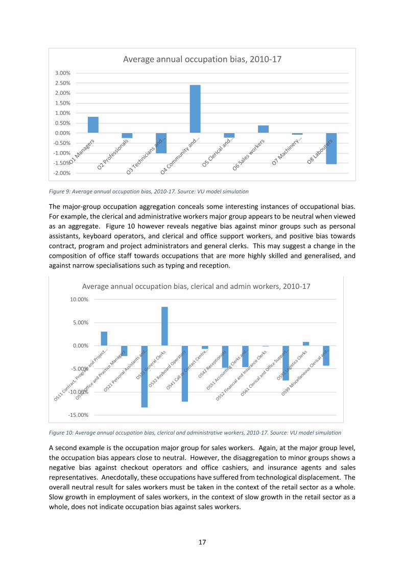
response to changes in technologies or tastes. Figure 9 shows that the positive occupational bias over
2010 to 2017 existed in favour of community and personal services workers and managers, while
labourers and technicians and trades workers suffered negative bias. This is broadly consistent with
the “Oxford List” (Frey and Osborne, 2013) which ranks occupations according to their susceptibility
to automation.
17
Figure 9: Average annual occupation bias, 2010-17. Source: VU model simulation
The major-group occupation aggregation conceals some interesting instances of occupational bias.
For example, the clerical and administrative workers major group appears to be neutral when viewed
as an aggregate. Figure 10 however reveals negative bias against minor groups such as personal
assistants, keyboard operators, and clerical and office support workers, and positive bias towards
contract, program and project administrators and general clerks. This may suggest a change in the
composition of office staff towards occupations that are more highly skilled and generalised, and
against narrow specialisations such as typing and reception.
Figure 10: Average annual occupation bias, clerical and administrative workers, 2010-17. Source: VU model simulation
A second example is the occupation major group for sales workers. Again, at the major group level,
the occupation bias appears close to neutral. However, the disaggregation to minor groups shows a
negative bias against checkout operators and office cashiers, and insurance agents and sales
representatives. Anecdotally, these occupations have suffered from technological displacement. The
overall neutral result for sales workers must be taken in the context of the retail sector as a whole.
Slow growth in employment of sales workers, in the context of slow growth in the retail sector as a
whole, does not indicate occupation bias against sales workers.
-2.00%
-1.50%
-1.00%
-0.50%
0.00%
0.50%
1.00%
1.50%
2.00%
2.50%
3.00%
Average annual occupation bias, 2010-17
-15.00%
-10.00%
-5.00%
0.00%
5.00%
10.00%
Average annual occupation bias, clerical and admin workers, 2010-17

18
Figure 11: Average annual occupation bias, sales workers, 2010-17. Source: VU model simulation
2.2.3.2 Demand for goods and services
Demand for goods and services in the VU model is derived by adding together demand by industries,
investors, households, the rest of the world (exports) and government, where each of these agents
has its own demand function. The demand functions include explanatory variables such as:
- industry output and investment (the output of an industry will determine its demand for
goods and services inputs, likewise its investment expenditure will determine demand for
inputs to capital creation, such as construction or machinery);
- household income (to determine household demand for commodities);
- government expenditure decisions;
- economic growth in export destinations;
- prices (this is particularly important for export demand);
- prices of competing imports, which are assumed to be substitutable for local varieties; and
- changes in tastes (households), technology (industries), and preferences for substitution to
imports (all users).
The model is calibrated such that all markets clear, so demand for each commodity must equate to
industry supply. The VU historical simulation is run to reproduce observed industry employment over
the period 2010-17, which is closely related to industry output. The historical simulation also
reproduces observed import volumes for manufactured commodities. With most explanatory
variables listed above already tied down by macroeconomic conditions, the observations for industry
employment and commodity imports are accommodated by changes to household tastes and industry
technologies, and changes to import substitution preferences.
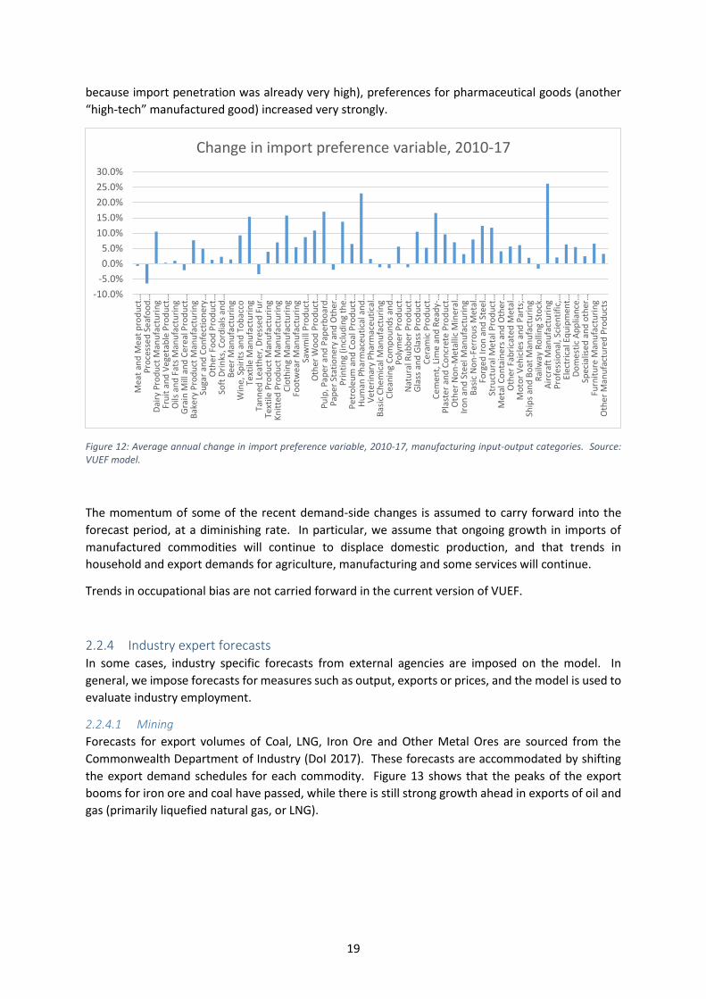
The historical simulation revealed interesting results for import preferences for manufactured
commodities, illustrated in Figure 12. Positive results indicate an increased preference for imports.
The historical simulation reveals positive results for almost all manufactured commodities. Overall,
results were larger for light manufactures and construction materials, and relatively small for food
products and high-tech equipment. However, there were some exceptions: among food products,
preferences clearly increased for imported dairy products, bakery products and wine, spirits and
tobacco. While preferences for imports of high-tech equipment increased only slightly (possibly
-5.00%
-4.00%
-3.00%
-2.00%
-1.00%
0.00%
1.00%
2.00%
3.00%
O611 InsuranceAgents and SalesRepresentatives
O612 Real EstateSales Agents
O621 SalesAssistants andSalespersons
O631 CheckoutOperators andOffice Cashiers
O639 MiscellaneousSales Support
Workers
Average annual occupation bias, sales workers, 2010-17
19
because import penetration was already very high), preferences for pharmaceutical goods (another
“high-tech” manufactured good) increased very strongly.
Figure 12: Average annual change in import preference variable, 2010-17, manufacturing input-output categories. Source: VUEF model.
The momentum of some of the recent demand-side changes is assumed to carry forward into the
forecast period, at a diminishing rate. In particular, we assume that ongoing growth in imports of
manufactured commodities will continue to displace domestic production, and that trends in
household and export demands for agriculture, manufacturing and some services will continue.
Trends in occupational bias are not carried forward in the current version of VUEF.
2.2.4 Industry expert forecasts In some cases, industry specific forecasts from external agencies are imposed on the model. In
general, we impose forecasts for measures such as output, exports or prices, and the model is used to
evaluate industry employment.
2.2.4.1 Mining
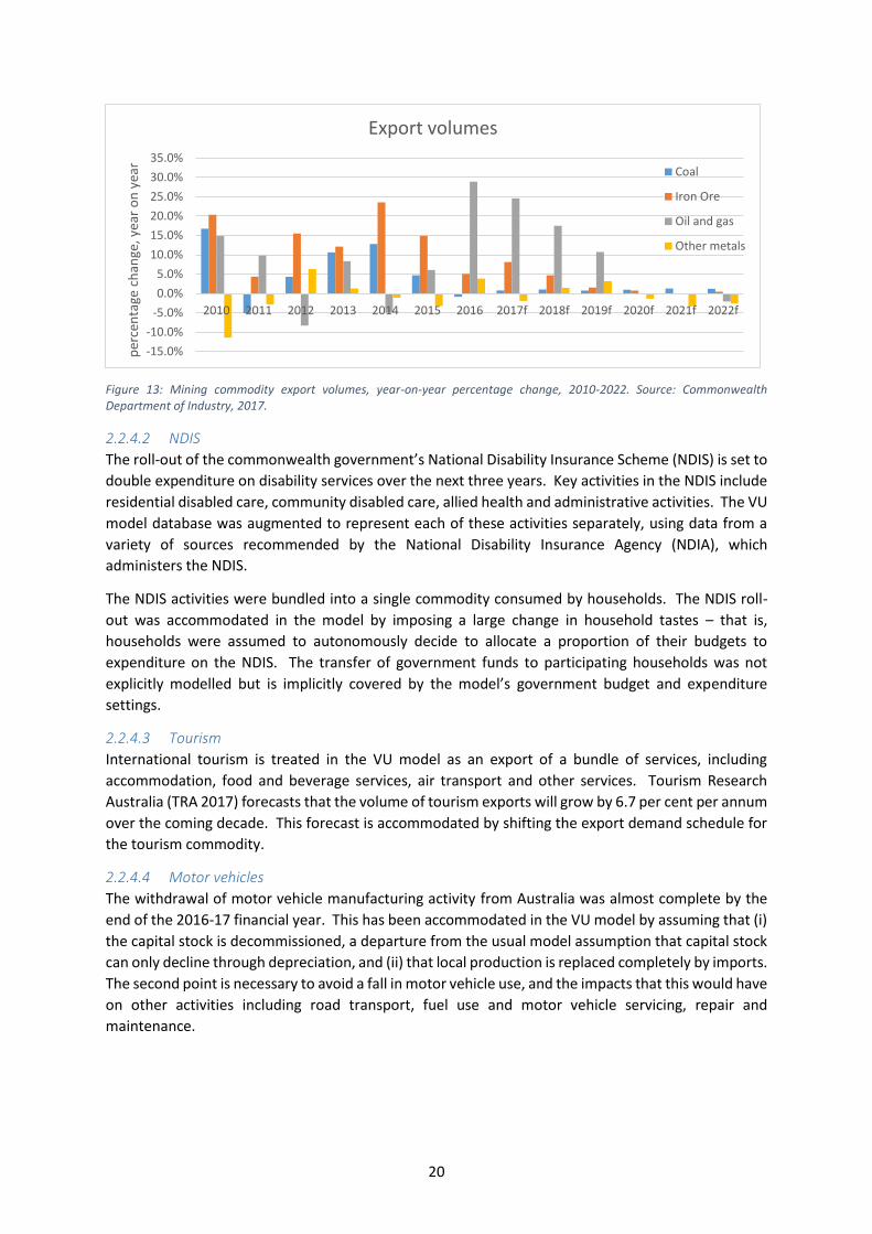
Forecasts for export volumes of Coal, LNG, Iron Ore and Other Metal Ores are sourced from the
Commonwealth Department of Industry (DoI 2017). These forecasts are accommodated by shifting
the export demand schedules for each commodity. Figure 13 shows that the peaks of the export
booms for iron ore and coal have passed, while there is still strong growth ahead in exports of oil and
gas (primarily liquefied natural gas, or LNG).
-10.0%
-5.0%
0.0%
5.0%
10.0%
15.0%
20.0%
25.0%
30.0%
Mea
t an
d M
eat
pro
du
ct…
Pro
cess
ed
Se
afo
od
…D
airy
Pro
du
ct M
anu
fact
uri
ng
Fru
it a
nd
Veg
etab
le P
rod
uct
…O
ils a
nd
Fat
s M
anu
fact
uri
ng
Gra
in M
ill a
nd
Cer
eal P
rod
uct
…B
ake
ry P
rod
uct
Man
ufa
ctu
rin
gSu
gar
and
Co
nfe
ctio
ner
y…O
ther
Fo
od
Pro
du
ct…
Soft
Dri
nks
, Co
rdia
ls a
nd
…B
eer
Man
ufa
ctu
rin
gW
ine,
Sp
irit
s an
d T
ob
acco
Text
ile M
anu
fact
uri
ng
Tan
ned
Lea
ther
, Dre
ssed
Fu
r…Te
xtile
Pro
du
ct M
anu
fact
uri
ng
Kn
itte
d P
rod
uct
Man
ufa
ctu
rin
gC
loth
ing
Man
ufa
ctu
rin
gFo
otw
ear
Man
ufa
ctu
rin
gSa
wm
ill P
rod
uct
…O
ther
Wo
od
Pro
du
ct…
Pu
lp, P
aper
an
d P
aper
bo
ard
…P
ape
r St
atio
ner
y an
d O
ther
…P
rin
tin
g (i
ncl
ud
ing
the
…P
etr
ole
um
an
d C
oal
Pro
du
ct…
Hu
man
Ph
arm
aceu
tica
l an
d…
Vet
eri
nar
y P
har
mac
euti
cal…
Bas
ic C
he
mic
al M
anu
fact
uri
ng
Cle
anin
g C
om
po
un
ds
and
…P
oly
me
r P
rod
uct
…N
atu
ral R
ub
ber
Pro
du
ct…
Gla
ss a
nd
Gla
ss P
rod
uct
…C
eram
ic P
rod
uct
…C
emen
t, L
ime
and
Re
ady-
…P
last
er a
nd
Co
ncr
ete
Pro
du
ct…
Oth
er N
on
-Met
allic
Min
eral
…Ir
on
an
d S
teel
Man
ufa
ctu
rin
gB
asic
No
n-F
erro
us
Met
al…
Forg
ed
Iro
n a
nd
Ste
el…
Stru
ctu
ral M
eta
l Pro
du
ct…
Met
al C
on
tain
ers
and
Oth
er…
Oth
er F
abri
cate
d M
etal
…M
oto
r V
ehic
les
and
Par
ts;…
Ship
s an
d B
oat
Man
ufa
ctu
rin
gR
ailw
ay R
olli
ng
Sto
ck…
Air
craf
t M
anu
fact
uri
ng
Pro
fess
ion
al, S
cien
tifi
c,…
Elec
tric
al E
qu
ipm
ent…
Do
me
stic
Ap
plia
nce
…Sp
ecia
lised
an
d o
ther
…Fu
rnit
ure
Man
ufa
ctu
rin
gO
ther
Man
ufa
ctu
red
Pro
du
cts
Change in import preference variable, 2010-17
20
Figure 13: Mining commodity export volumes, year-on-year percentage change, 2010-2022. Source: Commonwealth Department of Industry, 2017.
2.2.4.2 NDIS
The roll-out of the commonwealth government’s National Disability Insurance Scheme (NDIS) is set to
double expenditure on disability services over the next three years. Key activities in the NDIS include
residential disabled care, community disabled care, allied health and administrative activities. The VU
model database was augmented to represent each of these activities separately, using data from a
variety of sources recommended by the National Disability Insurance Agency (NDIA), which
administers the NDIS.
The NDIS activities were bundled into a single commodity consumed by households. The NDIS roll-
out was accommodated in the model by imposing a large change in household tastes – that is,
households were assumed to autonomously decide to allocate a proportion of their budgets to
expenditure on the NDIS. The transfer of government funds to participating households was not
explicitly modelled but is implicitly covered by the model’s government budget and expenditure
settings.
2.2.4.3 Tourism
International tourism is treated in the VU model as an export of a bundle of services, including
accommodation, food and beverage services, air transport and other services. Tourism Research
Australia (TRA 2017) forecasts that the volume of tourism exports will grow by 6.7 per cent per annum
over the coming decade. This forecast is accommodated by shifting the export demand schedule for
the tourism commodity.
2.2.4.4 Motor vehicles
The withdrawal of motor vehicle manufacturing activity from Australia was almost complete by the
end of the 2016-17 financial year. This has been accommodated in the VU model by assuming that (i)
the capital stock is decommissioned, a departure from the usual model assumption that capital stock
can only decline through depreciation, and (ii) that local production is replaced completely by imports.
The second point is necessary to avoid a fall in motor vehicle use, and the impacts that this would have
on other activities including road transport, fuel use and motor vehicle servicing, repair and
maintenance.
-15.0%
-10.0%
-5.0%
0.0%
5.0%
10.0%
15.0%
20.0%
25.0%
30.0%
35.0%
2010 2011 2012 2013 2014 2015 2016 2017f 2018f 2019f 2020f 2021f 2022f
per
cen
tage
ch
ange
, yea
r o
n y
ear
Export volumes
Coal
Iron Ore
Oil and gas
Other metals

21
2.3 Qualification supply estimates and cohort model
2.3.1 Historical data Data from the ABS survey of education and work is used to project skill acquisition over the forecast
period. Using annual data from 2008 to 2016, changes in head-counts of skill level and field are
ascribed to a cohort effect and an acquisition effect.
The cohort effect is what would occur if everyone in the workforce retained his or her existing
qualification level and field from the previous year. This is calculated by simply assuming that each
individual in the workforce is one year older than he/she was in the previous year. In ten-year age
cohorts for example, one tenth of the age group is assumed to move into the next age group.
The acquisition effect is the difference between the cohort effect and the observed qualification levels
and fields. For example, every year a group of workers from the 15-19 age group enters the 20-24 age
group. Very few (less than 1%) of these workers have a Bachelor’s degree, yet around 15 per cent of
the 20-24 age group have a Bachelor’s degree. This difference between the cohort effect and
observation is attributed to acquisition of new qualifications in the 20-24 age group. The term
“acquisition” is used to refer to the labour force as a whole. That is, the labour force acquires a new
Bachelor degree worker if he or she is a new entrant to the labour force (regardless of whether the
qualification is newly acquired by the individual), or if an existing participant in the labour force
upgrades his or her qualification to Bachelor’s degree.
Figure 14: Net share of workforce with new qualification, level of qualification by age and sex, average 2008-2016. Source ABS 6227.0 and author's calculations
Figure 14 shows the proportion of the workforce in each demographic that is assumed to have
acquired a new qualification in the last year, averaged over the period 2008 to 2016. From Figure 14
we can see that this proportion is highest among younger workers, and falls away significantly after
the age of 35 for both men and women. At all ages however, the majority of workers carry over their
qualification from the previous year.
Workers aged 19 and below acquiring new qualifications are most likely to acquire a Certificate I-IV or
an Advanced Diploma. Males aged 20 to 24 are more likely than females of the same age to acquire
a Certificate, while females in this age group are more likely to obtain a Bachelor’s degree. Bachelor’s
-2%
0%
2%
4%
6%
8%
10%
12%
14%
15-19 15-19 20-24 20-24 25-34 25-34 35-44 35-44 45-54 45-54 55+ 55+
M F M F M F M F M F M F
Net share of workforce with new qualification
Certificate I-IV
Advanced diploma
Bachelor degree
Graduate diploma
Postgraduate

22
degrees are generally obtained by workers of both sexes between the ages of 20 and 34, while
postgraduate degrees are more likely to be acquired after the age of 25.
Figure 15: Net share of workforce with new qualification, field of qualification by age and sex, average 2008-2016. Source ABS 6227.0 and author's calculations
The interpretation of Figure 15 is similar to that of Figure 14, except that Figure 15 shows qualification
acquisition by main field of study. There are clear differences in fields of study by age group and sex.
At every age, engineering, architecture and building and IT qualifications are more popular with males,
while qualifications in health and society and culture are more popular with females. Before the age
of 34, management or commerce qualifications are more popular with females. Beyond 35,
management or commerce qualifications begin to make up a significant proportion of qualification
acquisition for males. Qualification acquisitions in food and hospitality are significant in the 15-19 age
group.
In principle the totals in Figures 14 and 15 should match. However, an exact match is not possible. As
we are unable to follow individual workers through the sample, individual behaviour may only be
inferred from changes in demographic cohorts. If, for example, an individual who already has a
Bachelor’s degree in Engineering acquires a Bachelor’s degree in Management, this will appear as a
skill acquisition in the qualification field data (a new qualification in Management), but not in the
qualification levels data, as the worker has not changed the level of his or her qualification.
2.3.2 Skill forecasts The estimates for qualification acquisition by age and sex are interfaced with population projections
by age and sex to form the skill projections that are input into the VU model. The cohort effect is
calculated by assuming that a proportion of each demographic will retain their qualification level from
-2%
0%
2%
4%
6%
8%
10%
12%
14%
16%
15-19 15-19 20-24 20-24 25-34 25-34 35-44 35-44 45-54 45-54 55+ 55+
M F M F M F M F M F M F
Net share of workforce with new qualification
Food/Hospitality
Creative arts
Society/Culture
Management/Commerce
Education
Health
Agriculture
Architecture/Building
Engineering
IT
Science

23
one year to the next. The acquisition effect is calculated by assuming that a proportion of each
demographic will acquire new qualifications as indicated above.
Figure 16 shows that growth rates will be greater, the higher the skill level, with growth in
postgraduate qualifications the highest. Note however that growth rates can paint a misleading
picture, particularly where the base is small. Figure 17 shows the composition of employment growth
over the forecast period, illustrating more clearly that the largest contribution (by level) will be from
bachelor’s degrees, and the largest contributions (by field) will be from management and commerce,
and society and culture.
Figure 16: Projected employment growth rates by skill, 2017-2025. Source: author's calculations
Figure 17: Projected contribution to employment growth by skill, 2017-2025. Source: author's calculations
-1.00%
0.00%
1.00%
2.00%
3.00%
4.00%
5.00%
6.00%
Ave
rage
an
nu
al g
row
th, 2
01
7-2
02
5
Employment growth rates Postgraduate
Graduate diploma
Bachelor degree
Advanced diploma
Certificate I-IV
No post-school
-10.00%
-8.00%
-6.00%
-4.00%
-2.00%
0.00%
2.00%
4.00%
6.00%
8.00%
10.00%
12.00%
Co
ntr
ibu
tio
n t
o g
row
th, 2
01
7-2
02
5
Contributions to employment growthPostgraduate
Graduate diploma
Bachelor degree
Advanced diploma
Certificate I-IV
No post-school

24
2.4 Regional forecasts Regional estimates are generated using a tops-down regional disaggregation technique. Giesecke and
Madden (2013a, 2013b) give a detailed technical description of the methodology. The essence of it is
that every sector can be classified as either “national” or “local”. The performance of “national”
sectors is the same across all regions, for example, if the national model finds that output of “Chemical
Manufacturing” declines by 10 per cent, then it declines by 10 per cent in every region. The
performance of “local” sectors is dependent on the performance of the region in which they are
situated. In our example, local industries in a region heavily dependent on the declining “Chemical
Manufacturing” sector will also decline. This regional modelling method has built-in checks and
balances, so that regional activity adds to national activity in every sector.
National sectors are assumed to be those which produce traded commodities. For these sectors, the
region of origin is assumed not to be an important determinant of output. With an extremely
disaggregated industrial structure, the risk of the inappropriate attribution of activities to the regions
is low. For example, it would be incorrect to attribute net growth in “agriculture” uniformly across all
regions if in fact activity in dairy had increased while wheat had declined. With a more disaggregated
approach, we can correctly attribute dairy and wheat separately to their appropriate regions, perhaps
finding that agriculture in dairy-intensive regions increases while agriculture in wheat-intensive
regions declines.
The main data source for regional estimation is the census. Employment classified by industry and
region gives a good indication of the regional distribution of industries. The current version of the
CoPS top-down regional disaggregation model is based on census data for ASGS SA4 regions, with each
capital city region aggregated into a single region. Capital city regions are aggregated to minimise
leakage due to differences in workers’ place of residence and place of work.
The tops-down methodology is supplemented with the use of region-specific forecasts of population.
Along with regional industry activity, the regional population forecasts from the various state
demographers are used to explain household consumption, and hence some local industry activity, in
the regional model.
In addition to population forecasts, VUEF adopts aggregate employment forecasts from NSW and WA.
The WA forecast is adopted from the WA state budget. The NSW forecast, provided by the
Department of Premier and Cabinet, are derived from the NSW Treasury’s long term fiscal pressures
model, and underpinned by the NSW Intergeneration Report (NSW Treasury 2016). Average annual
employment growth in NSW over the VUEF forecast period (2018-2025) is forecast by NSW Treasury
to be 1.11%, almost half of a percentage point below the annual growth rate forecast of 1.57% for
national employment. Because of the size of the NSW economy, one implication of this is that forecast
annual growth in the remaining states is relatively strong, averaging 1.80%.

25
3 The employment forecasts
3.1 Industries
3.1.1 Overview VUEF industry forecasts are calculated at the 3-digit ANZSIC group level, which comprises 214
industries. Figure 17 summarises these forecasts into the 19 ANZSIC divisions. The vertical bar at
2017 marks the transition from historical to forecast employment.
Throughout the 1990’s, manufacturing was the nation’s largest employer. Since 2002 it has been
overtaken, first by retail, and next by the rapidly-expanding health sector, which is now 75% larger
than manufacturing. Construction passed manufacturing in 2010, close to the height of the mining-
related construction boom, and more recently, employment in both professional, scientific and
technical services and education and training has overtaken manufacturing. These changes are an
illustration of the changing nature of employment in Australia, which has become distinctly more
service-oriented as a result of strong income growth, changes in technology, and greater
manufacturing capacity and better transport links to many of our Asian trading partners.
Figure 18: National employment by industry division (historical data is smoothed), 1992-2025. Sources: ABS (1992-2017) and VUEF model (2018-2025)
0
1
0
500
1000
1500
2000
2500
19
92
19
93
19
94
19
95
19
96
19
97
19
98
19
99
20
00
20
01
20
02
20
03
20
04
20
05
20
06
20
07
20
08
20
09
20
10
20
11
20
12
20
13
20
14
20
15
20
16
20
17
20
18
f
20
19
f
20
20
f
20
21
f
20
22
f
20
23
f
20
24
f
20
25
f
Emp
loym
ent
(th
ou
san
d p
erso
ns)
National industry division employment, historical and forecast
A Agriculture, Forestry and FishingB MiningC ManufacturingD Electricity, Gas, Water and Waste ServicesE ConstructionF Wholesale TradeG Retail TradeH Accommodation and Food ServicesI Transport, Postal and WarehousingJ Information Media and TelecommunicationsK Financial and Insurance ServicesL Rental, Hiring and Real Estate ServicesM Professional, Scientific and Technical ServicesN Administrative and Support ServicesO Public Administration and SafetyP Education and TrainingQ Health Care and Social AssistanceR Arts and Recreation ServicesS Other Services

26
The pace of industry employment growth will continue to change and vary between industries through
the forecast period. The more significant variations and changes are listed in Table 3 under three
categories: the strong growth industries, the slow growth industries, and the improving industries, for
which a reversal of recent declining in growth is forecast. Comment on this selection of industries
follow.
Strong growth Slow growth Improving growth
M Professional, Scientific and Technical Services P Education and Training Q Health Care and Social Assistance
B Mining E Construction H Accommodation and Food Services O Public Administration and Safety
A Agriculture, Forestry and Fishing C Manufacturing F Wholesale Trade
Table 3: Key industry growth forecasts. Source: VUEF model
3.1.2 Strong growth industries Industry divisions M, P, and Q are forecast to have the strongest employment growth through the
forecast period. These divisions are made up of service industries that face relatively low technological
disruption to employment, and relatively low import competition. All three divisions employ highly
qualified workers and are well-suited to a workforce that is supplying a growing proportion of degree-
qualified workers.
Growth rates for these industries do not differ greatly from recent performance. Continued strong
growth in Division Q (Health and social services) will cement its position as the nation’s largest
employer. An acceleration in Division Q employment growth in the near term reflects the
implementation phase of the NDIS.
The “strong growth” industry divisions accounted for 29 per cent of Australian jobs in 2017, and are
forecast to account for 32 per cent by 2025. These three divisions are forecast to add more than 800
thousand jobs over the eight-year forecast period, accounting for more than half of national
employment growth.
3.1.3 Slow growth industries All of the “slow growth” industries are forecast to experience growth rates that are both lower than
the national average, and lower than they have been in recent history.
Jobs in Division B (Mining) accounted for around 1 per cent of Australian employment throughout the
1990’s and early 2000’s. It climbed to above 2 per cent from around 2012 to 2016. Over the forecast
period, mining export volumes will be strong. However, mining activity is not very labour intensive,
and much of the expansion will be facilitated not by a larger labour force, but by capital installed over
the last decade. The mining industry’s share of national employment will fall from its current level of
1.9 per cent to around 1.65 per cent over the forecast period.
The growth rate for employment in Division E (Construction) is forecast to remain below the national
average, as it has been for most of this decade. Throughout the 1990’s and early 2000’s, Division E
accounted for between 7 and 8 per cent of Australian jobs. During the mining construction boom
years, this increased to around 9 per cent. With a fairly bland forecast for investment, in contrast to
the sharp rise and fall that has occurred so far this decade (Figure 7), construction employment will
return to a slightly lower share of national employment, falling back to 8 per cent of national
employment over the forecast period.
27
Employment growth in Division H (Accommodation and Food services) is forecast to be weak, despite
strong growth forecasts for international tourism. While international tourism is beneficial to growth
in Division H, accommodation and food services depend primarily on the household sector, where
expenditure growth is relatively subdued. The impact of subdued growth in aggregate household
expenditure falls disproportionately on non-necessities such as accommodation and food services.
The impact of slow growth in domestic expenditure is also apparent in government expenditure, with
below-average employment growth forecast for Division O (Public Administration and Safety). Slow
growth in Division O is a consequence of the expenditure restraint assumed to achieve a return to
surplus on the government budget over the next four years.
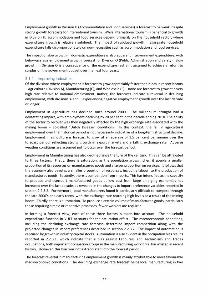
3.1.4 Improving industries Of the divisions where employment is forecast to grow appreciably faster than it has in recent history
– Agriculture (Division A), Manufacturing (C), and Wholesale (F) – none are forecast to grow at a very
high rate relative to national employment. Rather, the forecasts indicate a reversal in declining
employment, with divisions A and C experiencing negative employment growth over the last decade
or longer.
Employment in Agriculture has declined since around 2000. The millennium drought had a
devastating impact, with employment declining by 20 per cent in the decade ending 2010. The ability
of the sector to recover was then negatively affected by the high exchange rate associated with the
mining boom – so-called “Dutch Disease” conditions. In this context, the fall in agricultural
employment over the historical period is not necessarily indicative of a long-term structural decline.
Employment in agriculture is forecast to grow at an average of 1.5 per cent per annum over the
forecast period, reflecting strong growth in export markets and a falling exchange rate. Adverse
weather conditions are assumed not to occur over the forecast period.
Employment in Manufacturing has also declined since the turn of the century. This can be attributed
to three factors. Firstly, there is saturation: as the population grows richer, it spends a smaller
proportion of its resources on manufactured goods and a larger proportion on services. It follows that
the economy also devotes a smaller proportion of resources, including labour, to the production of
manufactured goods. Secondly, there is competition from imports. This has intensified as the capacity
to produce and transport manufactured goods at low cost from large emerging economies has
increased over the last decade, as revealed in the changes to import preference variables reported in
section 2.2.3.2. Furthermore, local manufacturers found it particularly difficult to compete through
the late 2000’s and early teens, with the exchange rate reaching high levels as a result of the mining
boom. Thirdly, there is automation. To produce a certain volume of manufactured goods, particularly
those requiring simple or repetitive processes, fewer workers are required.
In forming a forecast view, each of these three factors is taken into account. The household
expenditure function in VUEF accounts for the saturation effect. The macroeconomic conditions,
including the declining exchange rate forecast, determine import competition along with the
projected changes in import preferences described in section 2.2.3.2. The impact of automation is
captured by growth in industry capital stocks. Automation is also evident in the occupation bias results
reported in 2.2.3.1, which indicate that a bias against Labourers and Technicians and Trades
occupations, both important occupation groups in the manufacturing workforce, has existed in recent
history. However, this bias was not extrapolated into the forecast period.
The forecast reversal in manufacturing employment growth is mainly attributable to more favourable
macroeconomic conditions. The declining exchange rate forecast helps local manufacturing in two

28
ways: it makes manufacturing exports, such as many food products, more competitive on world
markets, and it makes import-competing activities, such as domestic appliances and furniture, more
competitive in the local market.
Furthermore, the import preference effects weaken as manufacturing becomes more specialised. For
example, employment in textiles, clothing and footwear has already declined so much that there is
little scope for it to decline further. At this stage, changes in import preferences become meaningless.
Similarly, employment in motor vehicle manufacturing has fallen as a result of the closures of several
major manufacturing plants, which limits the scope for it to fall further in the forecast period.
Without wishing to read too much into unfiltered data, there is some evidence that employment in
manufacturing is beginning to increase. ABS data shows that employment in manufacturing in May
2017 was over 900,000 persons, an increase of 47,000 persons over the previous 18 months. As shown
in Figure 19, this increase has yet to persist for long enough to show in the filtered series.
Figure 19: Employment in Division C Manufacturing, original and filtered data, 1991-2017. Source: ABS and author's calculations.
The Wholesale division (F) is closely linked to activity in manufacturing (both domestic and imported)
and agriculture. Wholesale is primarily a margin commodity. Almost 90 per cent of the sales income
in the Wholesale division is derived from facilitating sales of manufactured goods, with a further 7 per
cent derived from facilitating sales of agricultural output. Employment in wholesale tends to fluctuate
but a clear downward trend has been evident since around 2010. This is underscored by negative
growth in real per capita incomes and the consequent weak growth in demand for manufactured
products.
Employment growth in wholesale is forecast to turn around, with moderate but positive growth over
the forecast period in line with the forecast recoveries in manufacturing and agriculture.
In conclusion, macroeconomic conditions over the last decade in Australia have been characterised
by a boom and bust cycle in the terms of trade and investment leading to a temporarily high exchange
rate and a consequent temporary loss of competitiveness in manufacturing and agriculture. These
conditions exacerbated the weak performance of the agricultural sector caused by adverse weather
800
850
900
950
1000
1050
1100
1150
Au
g_1
99
1M
ay_1
99
2Fe
b_
19
93
No
v_1
99
3A
ug_
19
94
May
_19
95
Feb
_1
99
6N
ov_
19
96
Au
g_1
99
7M
ay_1
99
8Fe
b_
19
99
No
v_1
99
9A
ug_
20
00
May
_20
01
Feb
_2
00
2N
ov_
20
02
Au
g_2
00
3M
ay_2
00
4Fe
b_
20
05
No
v_2
00
5A
ug_
20
06
May
_20
07
Feb
_2
00
8N
ov_
20
08
Au
g_2
00
9M
ay_2
01
0Fe
b_
20
11
No
v_2
01
1A
ug_
20
12
May
_20
13
Feb
_2
01
4N
ov_
20
14
Au
g_2
01
5M
ay_2
01
6Fe
b_
20
17
Per
son
s em
plo
yed
(th
ou
san
ds)
Employment in Manufacturing
Original data
Filtered

29
conditions throughout the early 2000’s. The forecast period should see a return to more standard
macroeconomic conditions and a moderate recovery in these sectors.
However, the performance of the “improving industries”, which will add around 200,000 jobs over the
forecast period, is dwarfed by the “strong growth industries”, Health, Professional services and
Education, which will add more than 800,000 jobs and account for more than half of all employment
growth over the forecast period.
3.2 Occupations The VUEF model recognises that every industry has its own composition of employment by
occupation. For example, the predominant occupations of workers in the retail sector are the sales
occupations, while the predominant occupations of workers in the construction sector are the trade
and technician occupations. The evolution of aggregate employment by occupation is attributable to
changes in both the relative sizes of industries and changes in the composition of employment within
industries.
In 1991, the three largest occupation groups (ANZSCO major groups) in Australia – professionals,
technicians and trades workers, and clerical and administrative workers – were of a similar size, each
with 1.2 to 1.4 million workers. In 2017, these are still Australia’s three largest occupations, but
employment in the professional occupations is now around 80 per cent larger than employment in
either clerical and administrative occupations or technical and trades occupations. Employment in
the managerial occupations has also grown strongly to be on a par with the clerical and trades
occupations.
The very diverse Professional occupations group includes business professionals such as accountants
and sales and management professionals, legal professionals, health professionals including medical
and allied health practitioners and nurses, education professionals including teachers and university
lecturers, and professionals in design, engineering, science, transport, ICT and the arts. Past growth
in professional occupations has manifest not only in the strong-growth divisions Q (Health), M
(Professional services) and P (Education), but also outside these industries. Within some industry
divisions – particularly finance and insurance and public administration – the proportion of workers in
professional occupations has increased, while it has not fallen significantly in any sector.
Over the forecast period, as the workforce continues to become more educated, the professional
occupations are forecast to contribute the most to growth, accounting for 35 per cent of employment
growth, or almost 600,000 jobs.
Among the lower skilled occupations, growth in employment of labourers, machinery operators and
drivers and sales workers will continue to be sluggish. Low skilled workers may find more
opportunities in the community and personal services occupations in the strongly growing Health care
and social assistance sector.

30
Figure 20: National employment by occupation major group (historical data is smoothed), 1992-2025. Sources: ABS (1992-2017) and VUEF model (2018-2025)
3.3 Regions For each of the trade-exposed industries (known as “national” industries), the top down regional
disaggregation attributes national industry growth rates to the industry in every region in which it
operates. Regional growth rates for locally oriented industries, such as health and community
services, depend on regional population growth and the overall performance of the regional economy,
which is affected by the performance of the national industries operating in the region.
Figure 21 shows aggregate employment growth for capital cities and other areas for every state. In
most cases, the relatively high population forecasts and high concentration of the strong-growth
Professional Services industries in urban areas lead to stronger growth in the capital cities. The one
exception is Queensland, for which the population growth forecasts are strongest for regions other
than Brisbane, including Ipswich, Gold Coast, Moreton Bay North and Moreton Bay South.
As flagged earlier, forecasts for aggregate employment in NSW are calibrated to match exactly to
forecasts provided by the Department of Premier and Cabinet. The forecast for average annual
employment growth in NSW is just 1.11%, almost half of a percentage point below the annual growth
rate forecast of 1.57% for national employment. In order to accommodate the NSW growth forecast
in the context of a much higher national growth forecast, the original model estimates of growth in
most of the other states was adjusted upward.
An alternative approach would have been to have adjusted the national forecast downward.
However, strong justification would be required to deviate from the national forecast which is based
on ABS population forecasts and detailed projections of participation rates from the Commonwealth
Treasury. The approach will be revisited in the 2018 version of VUEF.
0
500
1000
1500
2000
2500
3000
3500
4000
19
92
19
93
19
94
19
95
19
96
19
97
19
98
19
99
20
00
20
01
20
02
20
03
20
04
20
05
20
06
20
07
20
08
20
09
20
10
20
11
20
12
20
13
20
14
20
15
20
16
20
17
20
18
f
20
19
f
20
20
f
20
21
f
20
22
f
20
23
f
20
24
f
20
25
f
Emp
loym
ent
(th
ou
san
d p
erso
ns)
National occupation employment, historical and forecast
O1 Managers
O2 Professionals
O3 Technicians and trades workers
O4 Community and personal service workers
O5 Clerical and administrative workers
O6 Sales workers
O7 Machinery operators and drivers
O8 Labourers

31
Figure 21: Employment growth rate forecasts, 2017-2025, capital cities and other regions. Source: VUEF Model
Figure 22 attests to the dominance of health, professional services and education in the capital cities
in employment growth over the forecast period. Of all jobs created in all industries and regions, one
in six will be in the health sector in capital cities. Health, professional services and education will be
the largest contributors to growth both within and outside capital cities, accounting for around half of
new jobs in both areas.
Figure 22: Contributions to employment growth, industry and region, 2017-2025. Source: VUEF model
0.00%
0.50%
1.00%
1.50%
2.00%
2.50%
3.00%
NSW Vic Qld SA WA Tas NT ACT National
Ave
rage
an
nu
al g
row
th r
ate,
20
17
-20
25
Employment growth rates, 2017-2025
Capital city
Other
Average
-2.0%
0.0%
2.0%
4.0%
6.0%
8.0%
10.0%
12.0%
14.0%
16.0%
18.0%
Contributions to employment growth, 2017-2025
Capital cities Other
32
4 Conclusions The Australian labour market grows at around 200,000 jobs per year. Over an eight-year forecast
horizon, VUEF provides a framework in which to determine the likely characteristics of the additional
1.6 million jobs that will be added to the workforce in the context of domestic economic growth,
technological change, a changing world economy and a more educated workforce.
We find the workforce will become more educated, with bachelor degree-qualified workers the
biggest growth category in the workforce in the forecast period. The proportion of the workforce with
no post-school qualification will decline, as retiring workers, many of whom hold no post-school
qualification, are replaced with younger workforce entrants who are more likely to obtain post-school
qualifications.
The macroeconomic environment will be characterised by moderate economic growth, with a lower
exchange rate facilitating a growing share of export activities including mining, agriculture and related
manufacturing activities, and education. The corollary of this is that growth in domestic expenditure
(both private and public) will be low relative to overall economic growth. Despite this, much of the
growth in employment will be concentrated in service industries with strong links to domestic
expenditure. This is because much of the export growth will occur in more capital-intensive activities
and have relatively little impact on employment.
Over the forecast period, three industry divisions will account for more than half of all employment
growth. Health, Professional services and Education are all service industries with strong indicators
of growth. All three sectors use the professional occupations, enabling them to absorb a large part of
the growing tertiary-qualified workforce. The implementation of the NDIS and the ageing of the
population underlie strong growth in the health sector, while the export markets for both education
and professional services sectors will expand as a result of a lower exchange rate. Professional
occupations will account for more than one-third of employment growth over the forecast period.
Following detailed population forecasts provided by state government agencies, the VUEF forecasts
concur that the majority of employment growth will occur in urban areas. The strong-growth services
sectors are important to growth in both capital cities and other areas; however, overall growth in
population and employment outside capital cities is slower. Both rural and urban areas will become
more reliant on the service sectors for employment over the forecast period.
The results reported in this paper represent only a summary of the detailed information contained in
the full VUEF database. This paper demonstrates the capacity of the VUEF model to generate detailed
forecasts in the context of a macroeconomic model of the Australian economy. The forecasts,
updated annually, are of considerable interest to state government agencies and the wider
community.

33
5 References ACT Treasury. (2013). Retrieved from ACT Population Projections:
https://apps.treasury.act.gov.au/demography/projections/act/total
Australian Bureau of Statistics. (2011). Census of Population and Housing, 2011. ABS.
Australian Bureau of Statistics. (2013). Input-Output Tables, 2009-10 (Cat. No. 5209.0.55.001).
Canberra: ABS.
Australian Bureau of Statistics. (2013). Population Projections, Australia, 2012 (base) to 2101 (Cat.
No. 3222.0). ABS.
Australian Bureau of Statistics. (2016). Education and Work, Australia, May 2016 (Cat. No. 6227.0).
ABS.
Australian Bureau of Statistics. (2017). Australian Demographic Statistics, Mar 2017 (Cat. No.
3101.0). ABS.
Australian Bureau of Statistics. (2017). Australian Industry, 2015-16 (Cat. No. 8155.0). ABS.
Australian Bureau of Statistics. (2017). Australian National Accounts: National Income, Expenditure
and Product, Jun 2017 (Cat. No. 5206.0). ABS.
Australian Bureau of Statistics. (2017). Balance of Payments and International Investment Position,
Australia, Jun 2017 (Cat. No. 5302.0). ABS.
Australian Bureau of Statistics. (2017). International Trade in Goods and Services, Australia, Jul 2017
(Cat. No. 5368.0). ABS.
Australian Bureau of Statistics. (2017). Labour Force, Australia, Detailed, Quarterly, May 2017 (Cat.
No. 6291.0.55.003). ABS.
Australian Bureau of Statistics. (2017). Labour Force, Australia, Jul 2017 (Cat. No. 6202.0). ABS.
Australian Bureau of Statistics. (2017). Wage Price Index, Australia, Jun 2017 (Cat. No. 6345.0). ABS.
Commonwealth Department of Industry. (2017). Resources and Energy Quarterly, March 2017.
Commonwealth of Australia. (2015). 2015 Intergenerational Report Australia in 2055. Canberra:
Commonwealth of Australia.
Commonwealth of Australia. (2017). Budget Strategy and Outlook: Budget Paper No. 1 2017-18.
Department of Environment, Land, Water and Planning, Victoria. (2016). Victoria in Future 2016.
Retrieved from http://www.delwp.vic.gov.au/victoria-in-future
Department of Planning, Transport and Infrastructure, SA. (2015). Population Projections for South
Australia and Statistical Divisions, 2011-41, September 2015 release. Retrieved from
https://data.sa.gov.au/data/dataset/population-projections-for-sa
Department of Planning, WA. (2015). Western Australia Tomorrow, Population Report No. 10,
Medium-term Forecasts for Western Australia 2014-2026 and Sub-regions 2016-2026.
Retrieved from https://www.planning.wa.gov.au/publications/6194.aspx
Department of Treasury and Finance, NT. (2014). Retrieved from Population Projections:
http://www.treasury.nt.gov.au/Economy/populationprojections/Pages/default.aspx

34
Dixon, J. (2016). Victoria University Employment Forecasts Information Paper. available from the
author on request.
Dixon, P. B., & Rimmer, M. T. (2002). Dynamic General Equilibrium Modelling for Forecasting and
Policy: A Practical Guide and Documentation of MONASH. North Holland Publishing
Company.
Dixon, P. B., Parmenter, B. R., Sutton, J., & Vincent, D. P. (1982). ORANI: A Multisectoral Model of the
Australian Economy. North Holland Publishing Company.
Frey, C. B., & Osborne, M. A. (2013). The future of employment: how susceptible are jobs to
computerisation. available at
http://www.oxfordmartin.ox.ac.uk/downloads/academic/future-of-employment.pdf
(accessed Nov. 8, 2016).
Giesecke, J. A., Tran, N. H., Meagher, G. A., & Pang, F. (2011). Growth and Change in the Vietnamese
Labour Market: A decomposition of forecast trends in employment over 2010-2020 . CoPS
Working Paper G-216 .
Giesecke, J. A., Tran, N. H., Meagher, G. A., & Pang, F. (2015). A decomposition approach to labour
market forecasting. Journal of the Asia Pacific Economy, 246-270.
Hodrick, R. J., & Prescott, E. C. (1997). Postwar U.S. Business Cycles: An Empirical Investigation.
Journal of Money, Credit and Banking, 29(1) pp. 1-16.
Meagher, G. A., & Pang, F. (2011). Labour Market Forecasting, Reliability and Workforce
Development. CoPS/IMPACT Working Paper Number G-225.
Meagher, G. A., & Parmenter, B. R. (1996). Future Workforce Skills: Projections with the MONASH
Model. Centre of Policy Studies, Monash University General Paper G-116.
Meagher, G. A., Adams, P. D., & Horridge, J. M. (2000). Applied General Equilibrium Modelling and
Labour Market Forecasting. Centre of Policy Studies, Monash University Preliminary Working
Paper IP-76.
NSW Treasury. (2016). Budget 2016-17 Budget Paper No. 5: Intergenerational Report.
NSW Treasury. (2017). Results from NSW Long Term Fiscal Pressures Model. not publically available.
Retrieved from NSW .
Queensland Government. (2013). Retrieved from Queensland Government population projections,
2013 edition: http://www.qgso.qld.gov.au/subjects/demography/population-projections/
Tasmanian Treasury. (2014). Retrieved from Population Projections:
http://www.treasury.tas.gov.au/economy/economic-data/2014-population-projections-for-
tasmania-and-its-local-government-areas
The Conference Board. (2016, May 23). Total Economy Database. Retrieved from
https://www.conference-board.org/data/economydatabase/index.cfm?id=27762
Tourism Research Australia. (2017). Tourism Forecasts 2017. Canberra.