Vibrations of wind-turbines considering soil...
28
Wind and Structures, Vol. 14, No. 2 (2011) 85-112 85 Vibrations of wind-turbines considering soil-structure interaction S. Adhikari * 1 and S. Bhattacharya 2a 1 College of Engineering, Swansea University, Singleton Park, Swansea SA2 8PP, UK 2 Department of Civil Engineering, University of Bristol, 2.37, Queen's Building, University Walk, Clifton, Bristol, BS8 1TR, UK (Received January 21, 2010, Accepted July 20, 2010) Abstract. Wind turbine structures are long slender columns with a rotor and blade assembly placed on the top. These slender structures vibrate due to dynamic environmental forces and its own dynamics. Analysis of the dynamic behavior of wind turbines is fundamental to the stability, performance, operation and safety of these systems. In this paper a simplied approach is outlined for free vibration analysis of these long, slender structures taking the soil-structure interaction into account. The analytical method is based on an Euler-Bernoulli beam-column with elastic end supports. The elastic end-supports are considered to model the flexible nature of the interaction of these systems with soil. A closed-form approximate expression has been derived for the first natural frequency of the system. This new expression is a function of geometric and elastic properties of wind turbine tower and properties of the foundation including soil. The proposed simple expression has been independently validated using an exact numerical method, laboratory based experimental measurement and field measurement of a real wind turbine structure. The results obtained in the paper shows that the proposed expression can be used for a quick assessment of the fundamental frequency of a wind turbine taking the soil-structure interaction into account. Keywords: mono-pile; natural frequency; beam theory; wind-turbine; soil stiffness. 1. Introduction It has been estimated that the world will require 50% more energy in 2030 than today (IEA, 2005). With the current policies on fossil fuels, greenhouse gas emissions will be 55% higher driving irreversible climate change and potentially triggering more extreme events such as floods, cyclones, heat waves, change in wind speed. A strategy is required to deliver both energy and climate security without compromising economic growth. Of all the sustainable sources of energy large offshore wind turbines have the proven potential to produce reliable quantities of renewable energy. Potential advantages of offshore turbines include: (a) Limited environmental impacts and out of sight; (b) High wind speed; (c) Available wave/current loading can also be harvested. Offshore wind turbine can be described as high slenderness low stiffness dynamical system involving complex interaction between the wind, wave and the soil. Due to the variety of cyclic and * Corresponding Author: Professor, E-mail: [email protected] a Senior Lecturer
Transcript of Vibrations of wind-turbines considering soil...
Wind and Structures, Vol. 14, No. 2 (2011) 85-112 85
Vibrations of wind-turbines consideringsoil-structure interaction
S. Adhikari*1 and S. Bhattacharya2a
1College of Engineering, Swansea University, Singleton Park, Swansea SA2 8PP, UK2Department of Civil Engineering, University of Bristol, 2.37, Queen's Building,
University Walk, Clifton, Bristol, BS8 1TR, UK
(Received January 21, 2010, Accepted July 20, 2010)
Abstract. Wind turbine structures are long slender columns with a rotor and blade assembly placed onthe top. These slender structures vibrate due to dynamic environmental forces and its own dynamics.Analysis of the dynamic behavior of wind turbines is fundamental to the stability, performance, operationand safety of these systems. In this paper a simplied approach is outlined for free vibration analysis ofthese long, slender structures taking the soil-structure interaction into account. The analytical method is basedon an Euler-Bernoulli beam-column with elastic end supports. The elastic end-supports are considered tomodel the flexible nature of the interaction of these systems with soil. A closed-form approximate expressionhas been derived for the first natural frequency of the system. This new expression is a function ofgeometric and elastic properties of wind turbine tower and properties of the foundation including soil. Theproposed simple expression has been independently validated using an exact numerical method, laboratorybased experimental measurement and field measurement of a real wind turbine structure. The results obtainedin the paper shows that the proposed expression can be used for a quick assessment of the fundamentalfrequency of a wind turbine taking the soil-structure interaction into account.
Keywords: mono-pile; natural frequency; beam theory; wind-turbine; soil stiffness.
1. Introduction
It has been estimated that the world will require 50% more energy in 2030 than today (IEA,
2005). With the current policies on fossil fuels, greenhouse gas emissions will be 55% higher
driving irreversible climate change and potentially triggering more extreme events such as floods,
cyclones, heat waves, change in wind speed. A strategy is required to deliver both energy and
climate security without compromising economic growth. Of all the sustainable sources of energy
large offshore wind turbines have the proven potential to produce reliable quantities of renewable
energy. Potential advantages of offshore turbines include: (a) Limited environmental impacts and out
of sight; (b) High wind speed; (c) Available wave/current loading can also be harvested.
Offshore wind turbine can be described as high slenderness low stiffness dynamical system
involving complex interaction between the wind, wave and the soil. Due to the variety of cyclic and
* Corresponding Author: Professor, E-mail: [email protected] Lecturer

86 S. Adhikari and S. Bhattacharya
dynamic loadings (arising from the rotor dynamics, out-of-balance masses, varying wind loading
intensity, wave loading), cyclic loads are induced in the foundations which are three dimensional in
nature. These are relatively new structures and there are no track record of long term performances
i.e., 20 years or beyond. Clearly, it is necessary to predict the long term performance of these
structures for the energy security from renewable sources.
The design of the foundations for offshore wind turbines remains a challenging task. Fig. 1 shows
a schematic diagram of an offshore wind turbine supported on a mono-pile, a particular type of
foundation. Mono-pile is a single slender member inserted deep into the ground to support the structure.
Typical mono-pile supporting a wind turbine is 3 to 4 m in diameter and 35 to 40 m long. Piles are
currently a popular choice for foundations possibly due to its long success in supporting offshore oil
platforms. Other forms of foundations that can be used to support wind turbines include suction
caissons i.e., an inverted bucket. The performance of suction caissons under the action of static,
cyclic and transient has been extensively researched; see for example Byrne and Houlsby (2003).
Currently, monopile foundation design for offshore wind turbines closely follows the pile design
for offshore fixed platforms. However, the offshore pile design concepts cannot be directly applied
to mono-pile design. There are signicant dierences between the two pile types:
(a) Offshore oil platform piles are longer (typically 60 m to 110 m), so degradation effects in the
upper soil layers due to cyclic loading are less severe.
(b) Offshore piles are also signicantly restrained from pile head rotation, whereas mono-piles are
free-headed.
The issue of cyclic strength degradation of the soil is taken empirically in offshore pile design. In
contrast, this is one of the important considerations in mono-pile design. Thus the two loading cases
Fig. 1 Mono-pile foundation to support offshore wind turbines and the proposed mathematical model for analysis.The translational spring constant kt and the rotational spring constant kr are used to model the soil-structure interaction. Experimental methods to obtain these two constants are discussed later in the paper
Vibrations of wind-turbines considering soil-structure interaction 87
are signicantly dierent, and it is not possible to rely on offshore pile design methods, since these
might produce an over-conservative or un-conservative design for mono-piles.
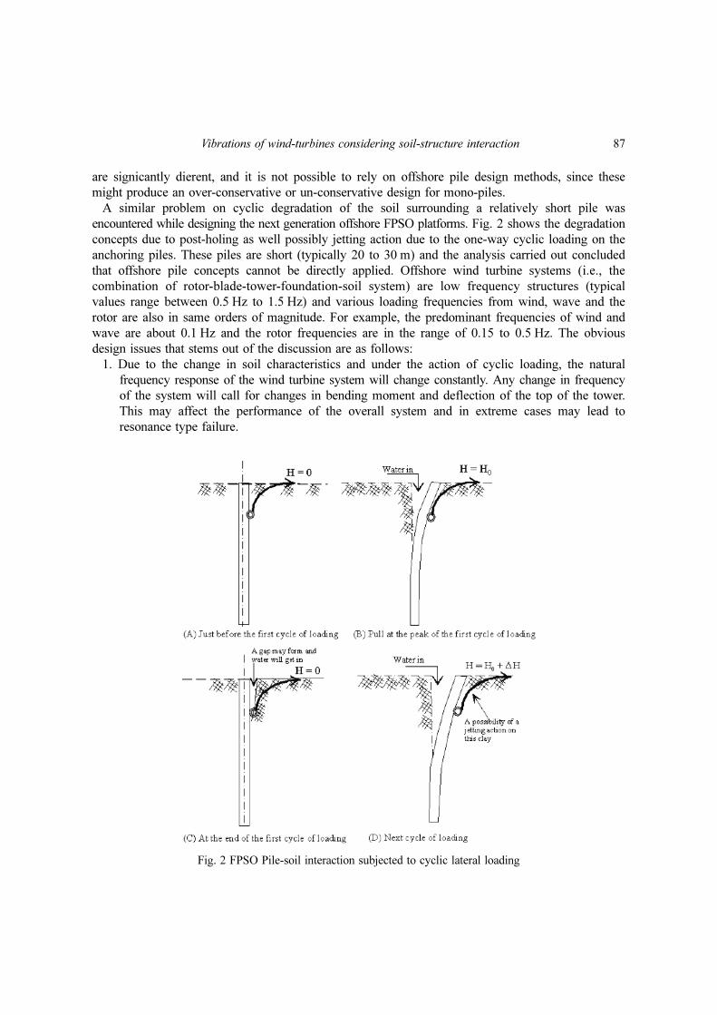
A similar problem on cyclic degradation of the soil surrounding a relatively short pile was
encountered while designing the next generation offshore FPSO platforms. Fig. 2 shows the degradation
concepts due to post-holing as well possibly jetting action due to the one-way cyclic loading on the
anchoring piles. These piles are short (typically 20 to 30 m) and the analysis carried out concluded
that offshore pile concepts cannot be directly applied. Offshore wind turbine systems (i.e., the
combination of rotor-blade-tower-foundation-soil system) are low frequency structures (typical
values range between 0.5 Hz to 1.5 Hz) and various loading frequencies from wind, wave and the
rotor are also in same orders of magnitude. For example, the predominant frequencies of wind and
wave are about 0.1 Hz and the rotor frequencies are in the range of 0.15 to 0.5 Hz. The obvious
design issues that stems out of the discussion are as follows:
1. Due to the change in soil characteristics and under the action of cyclic loading, the natural
frequency response of the wind turbine system will change constantly. Any change in frequency
of the system will call for changes in bending moment and deflection of the top of the tower.
This may affect the performance of the overall system and in extreme cases may lead to
resonance type failure.
Fig. 2 FPSO Pile-soil interaction subjected to cyclic lateral loading
88 S. Adhikari and S. Bhattacharya
2. Due to climate change, there may be a change in the wave loading, wind speed and more
extreme events (such as erratic wind gusts). It is necessary to predict the impact of these short
term extreme events.
An obvious solution is to design the wind turbine system so that the natural frequency of the
system does not come close to the forcing frequencies. The forcing frequencies are:
1. The frequency due to the wind and the wave
2. The rotor frequency often denoted by 1P
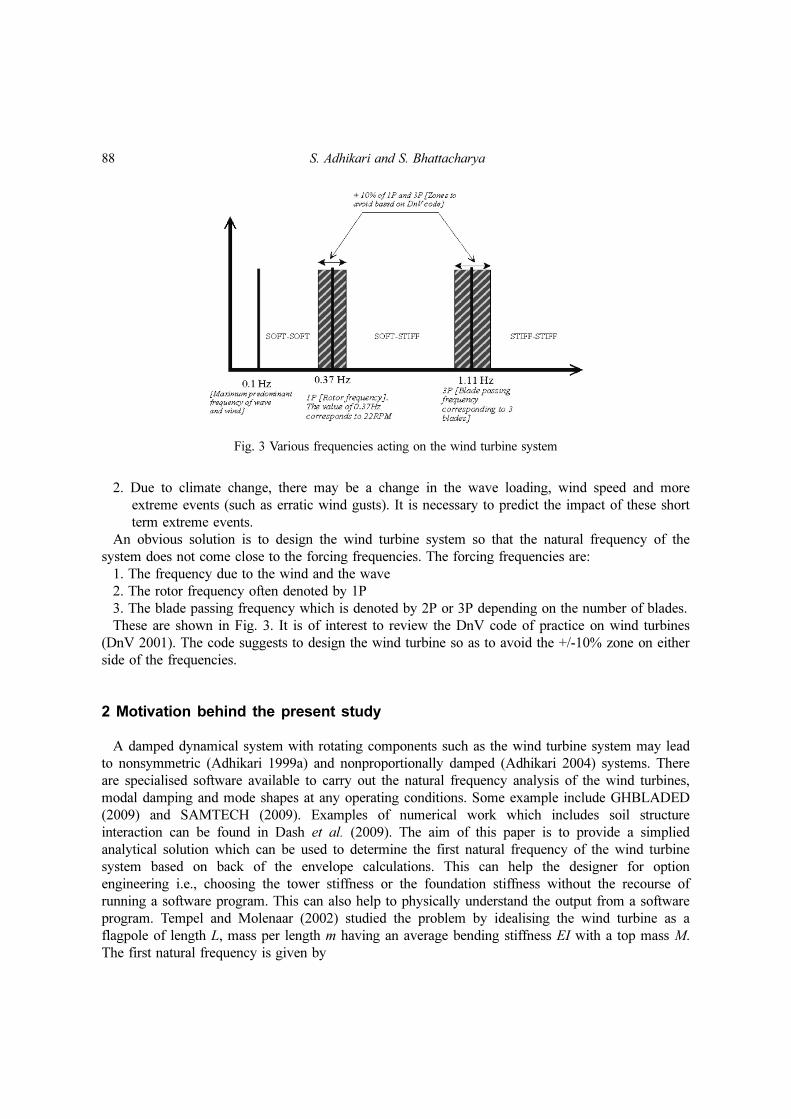
3. The blade passing frequency which is denoted by 2P or 3P depending on the number of blades.
These are shown in Fig. 3. It is of interest to review the DnV code of practice on wind turbines
(DnV 2001). The code suggests to design the wind turbine so as to avoid the +/-10% zone on either
side of the frequencies.
2 Motivation behind the present study
A damped dynamical system with rotating components such as the wind turbine system may lead
to nonsymmetric (Adhikari 1999a) and nonproportionally damped (Adhikari 2004) systems. There
are specialised software available to carry out the natural frequency analysis of the wind turbines,
modal damping and mode shapes at any operating conditions. Some example include GHBLADED
(2009) and SAMTECH (2009). Examples of numerical work which includes soil structure
interaction can be found in Dash et al. (2009). The aim of this paper is to provide a simplied
analytical solution which can be used to determine the first natural frequency of the wind turbine
system based on back of the envelope calculations. This can help the designer for option
engineering i.e., choosing the tower stiffness or the foundation stiffness without the recourse of
running a software program. This can also help to physically understand the output from a software
program. Tempel and Molenaar (2002) studied the problem by idealising the wind turbine as a
flagpole of length L, mass per length m having an average bending stiffness EI with a top mass M.
The first natural frequency is given by
Fig. 3 Various frequencies acting on the wind turbine system
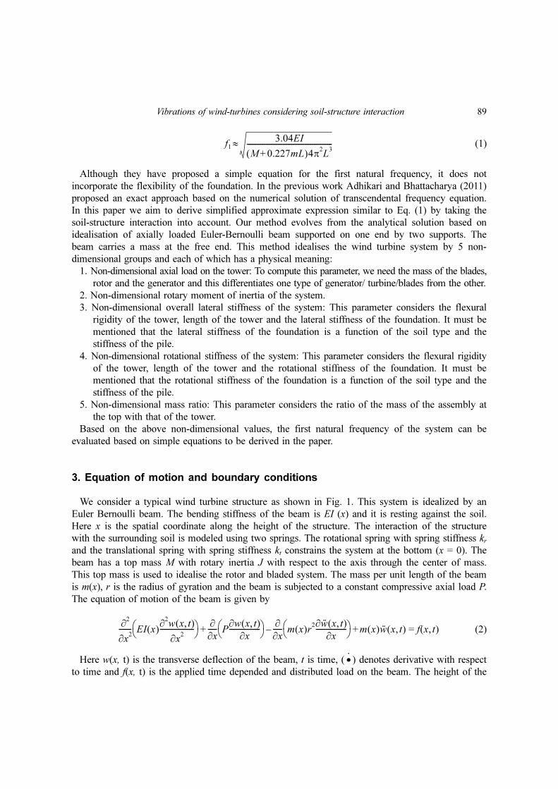
Vibrations of wind-turbines considering soil-structure interaction 89
(1)
Although they have proposed a simple equation for the first natural frequency, it does not
incorporate the flexibility of the foundation. In the previous work Adhikari and Bhattacharya (2011)
proposed an exact approach based on the numerical solution of transcendental frequency equation.
In this paper we aim to derive simplified approximate expression similar to Eq. (1) by taking the
soil-structure interaction into account. Our method evolves from the analytical solution based on
idealisation of axially loaded Euler-Bernoulli beam supported on one end by two supports. The
beam carries a mass at the free end. This method idealises the wind turbine system by 5 non-
dimensional groups and each of which has a physical meaning:
1. Non-dimensional axial load on the tower: To compute this parameter, we need the mass of the blades,
rotor and the generator and this differentiates one type of generator/ turbine/blades from the other.
2. Non-dimensional rotary moment of inertia of the system.
3. Non-dimensional overall lateral stiffness of the system: This parameter considers the flexural
rigidity of the tower, length of the tower and the lateral stiffness of the foundation. It must be
mentioned that the lateral stiffness of the foundation is a function of the soil type and the
stiffness of the pile.
4. Non-dimensional rotational stiffness of the system: This parameter considers the flexural rigidity
of the tower, length of the tower and the rotational stiffness of the foundation. It must be
mentioned that the rotational stiffness of the foundation is a function of the soil type and the
stiffness of the pile.
5. Non-dimensional mass ratio: This parameter considers the ratio of the mass of the assembly at
the top with that of the tower.
Based on the above non-dimensional values, the first natural frequency of the system can be
evaluated based on simple equations to be derived in the paper.
3. Equation of motion and boundary conditions
We consider a typical wind turbine structure as shown in Fig. 1. This system is idealized by an
Euler Bernoulli beam. The bending stiffness of the beam is EI (x) and it is resting against the soil.
Here x is the spatial coordinate along the height of the structure. The interaction of the structure
with the surrounding soil is modeled using two springs. The rotational spring with spring stiffness krand the translational spring with spring stiffness kt constrains the system at the bottom (x = 0). The
beam has a top mass M with rotary inertia J with respect to the axis through the center of mass.
This top mass is used to idealise the rotor and bladed system. The mass per unit length of the beam
is m(x), r is the radius of gyration and the beam is subjected to a constant compressive axial load P.
The equation of motion of the beam is given by
(2)
Here w(x, t) is the transverse deflection of the beam, t is time, ( ) denotes derivative with respect
to time and f(x, t) is the applied time depended and distributed load on the beam. The height of the
f13.04EI
M 0.227mL+( )4π2L3
--------------------------------------------------≈
∂2
∂x2
------- EI x( )∂2w x t,( )
∂x2
--------------------⎝ ⎠⎛ ⎞ ∂
∂x----- P
∂w x t,( )∂x
------------------⎝ ⎠⎛ ⎞ ∂
∂x----- m x( )r2∂w·· x t,( )
∂x------------------
⎝ ⎠⎛ ⎞ m x( )w·· x t,( )+–+ f x t,( )=
•·

90 S. Adhikari and S. Bhattacharya
structure is considered to be L. An Euler-Bernoulli beam with rotary inertia in Eq. (2) is also known
as the Rayleigh beam (Sheu and Yang 2005). Eq. (2) is a fourth-order partial differential equation
(Kreyszig 2006) and has been used extensively in literature for various problems, see for example,
Abramovich and Hamburger (1991), Adhikari and Bhattacharya (2008), Bhattacharya et al. (2009,
2008), Chen (1963), Elishakoff and Johnson (2005), Elishakoff and Perez (2005), Gurgoze (2005a),
Gurgoze and Erol (2002), Hetenyi (1946), Huang (1961), Laura and Gutierrez (1986), Oz (2003), Wu
and Chou (1998, 1999), Wu and Hsu (2006). Our aim is to obtain the natural frequencies of the system.
Here we develop an approach based on the non-dimensionalisation of the equation of motion (2).
Eq. (2) is a quite general equation. It is possible to consider any variation in the bending stiffness
EI(x) and mass density m(x) of the structure with height (such as a tapered column). Consideration
of such variation normally leads to the case where closed-form solutions are impossible to obtain
due to the complex nature of the resulting equations. For simplicity, we therefore assume a special
case where all properties are constant along the height of the structure. Noting that the properties
are not changing with x, Eq. (2) can be simplied as
(3)
The four boundary conditions associated with this equation can be expressed as
· Bending moment at x = 0
or (4)
· Shear force at x = 0
(5)
or
· Bending moment at x = L
or (6)
· Shear force at x = L
(7)
Assuming harmonic solution (the separation of the variables) we have
, (8)
Substituting this in the equation of motion and the boundary conditions, Eqs. (3) - (7), results
EI∂4w x t,( )
∂x4
-------------------- P∂2w x t,( )
∂x2
-------------------- mr2∂2w·· x t,( )
∂x2
-------------------- mw·· x t,( )+–+ f x t,( )=
EI∂2w x t,( )
∂x2
-------------------- kr
∂w x t,( )∂x
------------------– 0 x 0== EIw'' 0 t,( ) krw' 0 t,( )– 0=
EI∂3w x t,( )
∂x3-------------------- P
∂w x t,( )∂x
------------------ ktw x t,( ) mr2∂w·· x t,( )
∂x------------------–+ + 0 x 0=
=
EIw''' 0 t,( ) Pw' 0 t,( )+ ktw 0 t,( ) mr2∂w·· 0 t,( )
∂x------------------–+ 0=
EI∂2w x t,( )
∂x2-------------------- J
∂w·· x t,( )∂x
------------------+ 0 x L== EIw'' L t,( ) J∂w·· L t,( )
∂x-------------------+ 0=
EI∂3w x t,( )
∂x3-------------------- P
∂w x t,( )∂x
------------------ Mw·· x t,( )– mr2∂w·· x t,( )
∂x------------------–+ 0 x L==
EIw''' L t,( ) Pw' L t,( )+ Mw·· L t,( ) mr2∂w·· L t,( )
∂x-------------------–+ 0=
w x t,( ) W ξ( ) iωt exp= f x t,( ) F ξ( ) iωt exp= ξ x L⁄=
Vibrations of wind-turbines considering soil-structure interaction 91
(9)
(10)
(11)
(12)
(13)
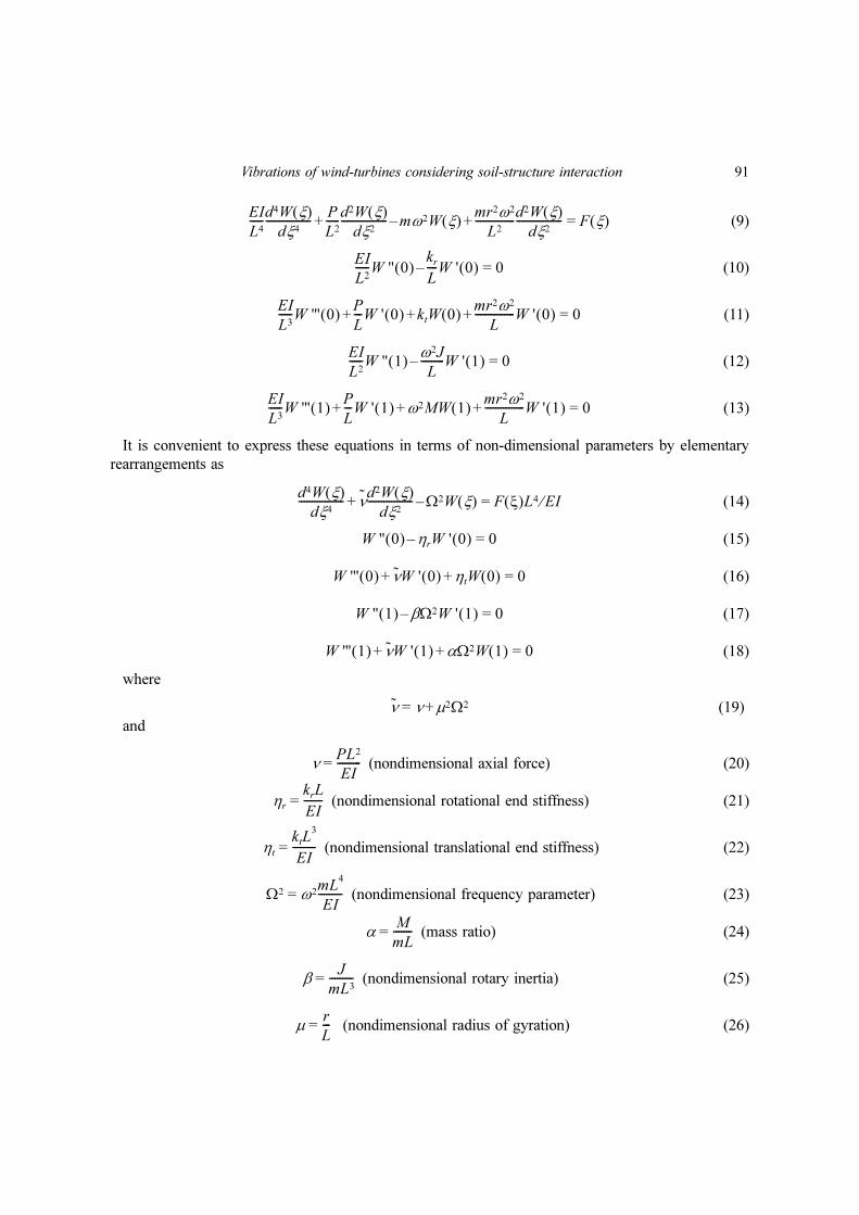
It is convenient to express these equations in terms of non-dimensional parameters by elementary
rearrangements as
(14)
(15)
(16)
(17)
(18)
where
(19)
and
(nondimensional axial force) (20)
(nondimensional rotational end stiffness) (21)
(nondimensional translational end stiffness) (22)
(nondimensional frequency parameter) (23)
(mass ratio) (24)
(nondimensional rotary inertia) (25)
(nondimensional radius of gyration) (26)
EI
L4-----
d4W ξ( )dξ4
-----------------P
L2-----
d2W ξ( )dξ2
----------------- mω2W ξ( )mr2ω2
L2---------------
d2W ξ( )dξ2
-----------------+–+ F ξ( )=
EI
L2-----W '' 0( )
kr
L----W ' 0( )– 0=
EI
L3-----W ''' 0( )
P
L---W ' 0( ) ktW 0( )
mr2ω2
L---------------W ' 0( )+ + + 0=
EI
L2-----W '' 1( ) ω2J
L---------W ' 1( )– 0=
EI
L3-----W ''' 1( )
P
L---W ' 1( ) ω2MW 1( )
mr2ω2
L---------------W ' 1( )+ + + 0=
d4W ξ( )dξ4
----------------- νd2W ξ( )
dξ2----------------- Ω2W ξ( )–+ F ξ( )L4 EI⁄=
W '' 0( ) ηrW ' 0( )– 0=
W ''' 0( ) νW ' 0( ) ηtW 0( )+ + 0=
W '' 1( ) βΩ2W ' 1( )– 0=
W ''' 1( ) νW ' 1( ) αΩ2W 1( )+ + 0=
ν ν µ2Ω2+=
νPL2
EI---------=
ηr
krL
EI-------=
ηt
ktL3
EI---------=
Ω2 ω2mL
4
EI---------=
αM
mL-------=
βJ
mL3---------=
µr
L---=
92 S. Adhikari and S. Bhattacharya
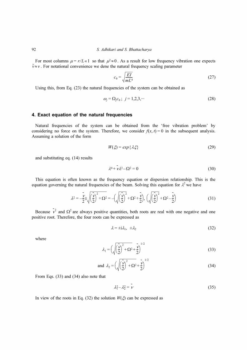
For most columns µ = so that . As a result for low frequency vibration one expects
. For notational convenience we dene the natural frequency scaling parameter
(27)
Using this, from Eq. (23) the natural frequencies of the system can be obtained as
; j = 1,2,3,··· (28)
4. Exact equation of the natural frequencies
Natural frequencies of the system can be obtained from the ‘free vibration problem’ by
considering no force on the system. Therefore, we consider f(x, t) = 0 in the subsequent analysis.
Assuming a solution of the form
(29)
and substituting eq. (14) results
(30)
This equation is often known as the frequency equation or dispersion relationship. This is the
equation governing the natural frequencies of the beam. Solving this equation for λ2 we have
(31)
Because and Ω2 are always positive quantities, both roots are real with one negative and one
positive root. Therefore, the four roots can be expressed as
λ = ±iλ1, ±λ2 (32)
where
(33)
and (34)
From Eqs. (33) and (34) also note that
(35)
In view of the roots in Eq. (32) the solution W(ξ) can be expressed as
r L⁄ 1« µ2 0≈v v≈
c0
EI
mL4---------=
ωj Ωjc0=
W ξ( ) λξ exp=
λ4 νλ2 Ω2–+ 0=
λ2ν
2---–
ν
2---⎝ ⎠⎛ ⎞
2
Ω2+±ν
2---⎝ ⎠⎛ ⎞
2
Ω2ν
2---+ +⎝ ⎠
⎛ ⎞– ν
2---⎝ ⎠⎛ ⎞
2
Ω2ν
2---–+⎝ ⎠
⎛ ⎞,= =
ν2
λ1
ν
2---⎝ ⎠⎛ ⎞
2
Ω2+ν
2---+⎝ ⎠
⎛ ⎞1 2⁄
=
λ2
ν
2---⎝ ⎠⎛ ⎞
2
Ω2+ν
2---+⎝ ⎠
⎛ ⎞1 2⁄
=
λ12 λ2
2– ν=
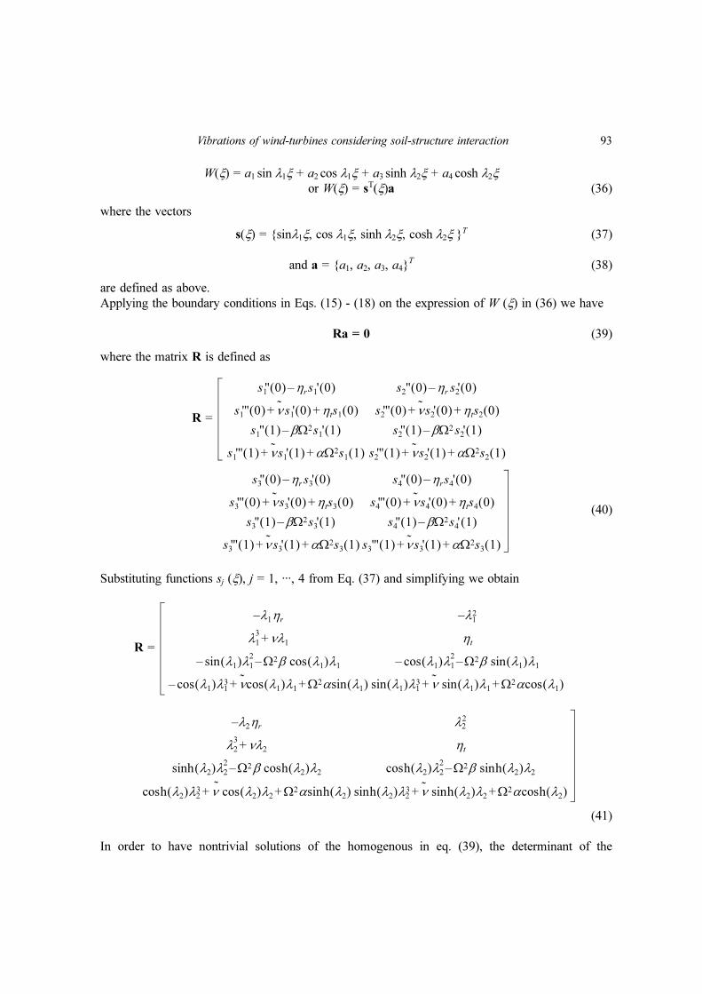
Vibrations of wind-turbines considering soil-structure interaction 93
W(ξ) = a1 sin λ1ξ + a2 cos λ1ξ + a3 sinh λ2ξ + a4 cosh λ2ξ
or W(ξ) = sT(ξ)a (36)
where the vectors
s(ξ) = sinλ1ξ, cos λ1ξ, sinh λ2ξ, cosh λ2ξ T (37)
and a = a1, a2, a3, a4T
(38)
are defined as above.
Applying the boundary conditions in Eqs. (15) - (18) on the expression of W (ξ) in (36) we have
Ra = 0 (39)
where the matrix R is defined as
R =
(40)
Substituting functions sj (ξ), j = 1, ···, 4 from Eq. (37) and simplifying we obtain
R =
(41)
In order to have nontrivial solutions of the homogenous in eq. (39), the determinant of the
s1'' 0( ) ηrs1' 0( )– s2'' 0( ) ηr s2' 0( )–
s1''' 0( ) ν s1' 0( ) ηts1 0( )+ + s2''' 0( ) ν s2' 0( ) ηts2 0( )+ +
s1'' 1( ) βΩ2s1' 1( )– s2'' 1( ) βΩ2 s2' 1( )–
s1''' 1( ) ν s1' 1( ) αΩ2s1 1( )+ + s2''' 1( ) ν s2' 1( ) αΩ2s2 1( )+ +
s3'' 0( ) ηr s3' 0( )– s4'' 0( ) ηrs4' 0( )–
s3''' 0( ) ν s3' 0( ) ηts3 0( )+ + s4''' 0( ) ν s4' 0( ) ηts4 0( )+ +
s3'' 1( ) βΩ2s3' 1( )– s4'' 1( ) βΩ2s4' 1( )–
s3''' 1( ) ν s3' 1( ) αΩ2s3 1( )+ + s3''' 1( ) ν s3' 1( ) αΩ2s3 1( )+ +
λ1ηr– λ12–
λ1
3νλ1+ ηt
λ1( )λ1
2sin– Ω2β λ1( )λ1cos– λ1( )cos λ1
2– Ω2β λ1( )λ1sin–
λ1( )λ13cos– ν λ1( )λ1cos Ω2α λ1( )sin+ + λ1( )sin λ1
3 ν λ1( )λ1sin Ω2α λ1( )cos+ +
λ2ηr– λ2
2
λ2
3νλ2+ ηt
h λ2( )λ2
2sin Ω2β h λ2( )λ2cos– h λ2( )cos λ2
2 Ω2β h λ2( )λ2sin–
h λ2( )λ23cos ν ˜ λ2( )λ2cos Ω2α h λ2( )sin+ + h λ2( )sin λ2
3 ν h λ2( )λ2sin Ω2α h λ2( )cos+ +

94 S. Adhikari and S. Bhattacharya
coefficients matrix should be zero, leading to the frequency equation
= 0 (42)
The natural frequencies can be obtained by solving Eq. (42) for Ω. Due to the complexity of this
transcendental equation it should be solved numerically. The details of the above can be found in
Adhikari and Bhattacharya (2011).
5. Approximate expression of the natural frequency
In the previous section exact expressions for the equation of the natural frequencies of the
combine wind turbine-soil system have been derived. Since only numerical solutions to these
transcendental equations are available, in this section we aim to derive approximate closed-form
solution with the aim of gaining more physical insights. For this application, the first mode of
vibration is the most signicant. As a result, we focus our attention on the first mode only.
In the first mode we can replace the distributed system by a single-degree-of-freedom system with
equivalent stiffness ke and equivalent mass Me as shown in Fig. 4. The first natural frequency is
given by
(43)
Following Table 8-8, case 1, page 158 of (Blevins 1984) for a cantilever beam carrying a tip mass
M, one has
Me = M + 0.24Mb = (α + 0.24)mL (44)
Representation of a cantilevered beam carrying a tip mass by an equivalent spring-mass system
has been discussed by Gurgoze (2005b). For our case the beam is resting on elastic foundation and
also have an end force. Therefore the cofficient 0.24 needs to be modied to take these effects into
account. We suppose that the equivalent mass can be represented by
Me = (α + γm)mL (45)
where γm is the mass correction factor.
R
ω12
ke
Me
------=
Fig. 4 Equivalent single-degree-of-freedom system for the first bending mode of the wind turbine
Vibrations of wind-turbines considering soil-structure interaction 95
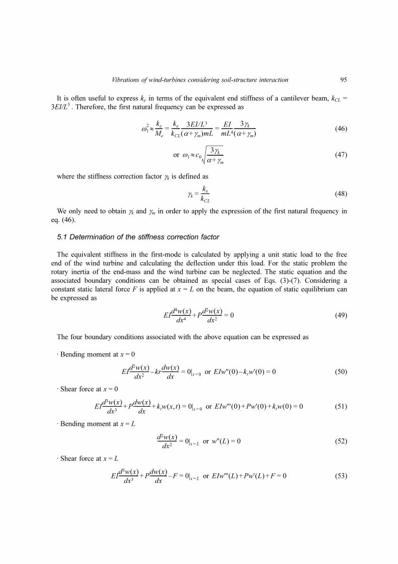
It is often useful to express ke in terms of the equivalent end stiffness of a cantilever beam, kCL =
3EI/L3 . Therefore, the first natural frequency can be expressed as
(46)
or (47)
where the stiffness correction factor γk is defined as
(48)
We only need to obtain γk and γm in order to apply the expression of the first natural frequency in
eq. (46).
5.1 Determination of the stiffness correction factor
The equivalent stiffness in the first-mode is calculated by applying a unit static load to the free
end of the wind turbine and calculating the deflection under this load. For the static problem the
rotary inertia of the end-mass and the wind turbine can be neglected. The static equation and the
associated boundary conditions can be obtained as special cases of Eqs. (3)-(7). Considering a
constant static lateral force F is applied at x = L on the beam, the equation of static equilibrium can
be expressed as
(49)
The four boundary conditions associated with the above equation can be expressed as
· Bending moment at x = 0
or (50)
· Shear force at x = 0
or (51)
· Bending moment at x = L
or (52)
· Shear force at x = L
or (53)
ω1
2 ke
Me
------≈ke
kCL
-------3EI L3⁄
α γm+( )mL--------------------------
EI
mL4---------
3γkα γm+( )
------------------= =
ω1 c0
3γkα γm+--------------≈
γkke
kCL
-------=
EId4w x( )
dx4---------------- P
d2w x( )dx2
----------------+ 0=
EId2w x( )
dx2---------------- kr
dw x( )dx
--------------– 0 x 0== EIw'' 0( ) krw' 0( )– 0=
EId3w x( )
dx3---------------- P
dw x( )dx
-------------- ktw x t,( )+ + 0 x 0== EIw''' 0( ) Pw' 0( ) ktw 0( )+ + 0=
d2w x( )dx2
---------------- 0 x L== w'' L( ) 0=
EId3w x( )
dx3---------------- P
dw x( )dx
-------------- F–+ 0 x L== EIw''' L( ) Pw' L( ) F+ + 0=

96 S. Adhikari and S. Bhattacharya
Using the non-dimensional length variable ξ and following the procedure outlined in the previous
section the governing equation boundary conditions can be expressed as
(54)
(55)
(56)
(57)
(58)
Considering a trial solution of the form in eq. (29) and substituting in the governing eq. (54)
results
or (59)
Solving this equation for λ2 we have
λ2 = 0 and λ = (60)
In view of the roots in in eq. (60) the solution W(ξ) can be expressed as
or (61)
where the vectors
(62)
and c = . (63)
Applying the boundary conditions in eqs. (55) - (58) on the expression of W(ξ) in (61) we have
Q c = f (64)
where
(65)
and the matrix
d4W ξ( )dξ4
----------------- νd2W ξ( )
dξ2-----------------+ 0=
W '' 0( ) ηrW ' 0( )– 0=
W ''' 0( ) νW ' 0( ) ηtW 0( )+ + 0=
W ' 1( ) 0=
W''' 1( ) νW' 1( )+FL3
EI---------–=
λ4
νλ2+ 0= λ2 λ2 ν+( ) 0=
i ν±
W ξ( ) c1 c2ξ c3 λξsin c4 λξcos+ + += W ξ( ) sT ξ( )c=
s ξ( ) 1 ξ λξsin λξcos, , , T=
c1 c2 c3 c4, , , T
f
0
0
0
FL3
EI---------–⎩ ⎭
⎪ ⎪⎪ ⎪⎨ ⎬⎪ ⎪⎪ ⎪⎧ ⎫
=
Vibrations of wind-turbines considering soil-structure interaction 97
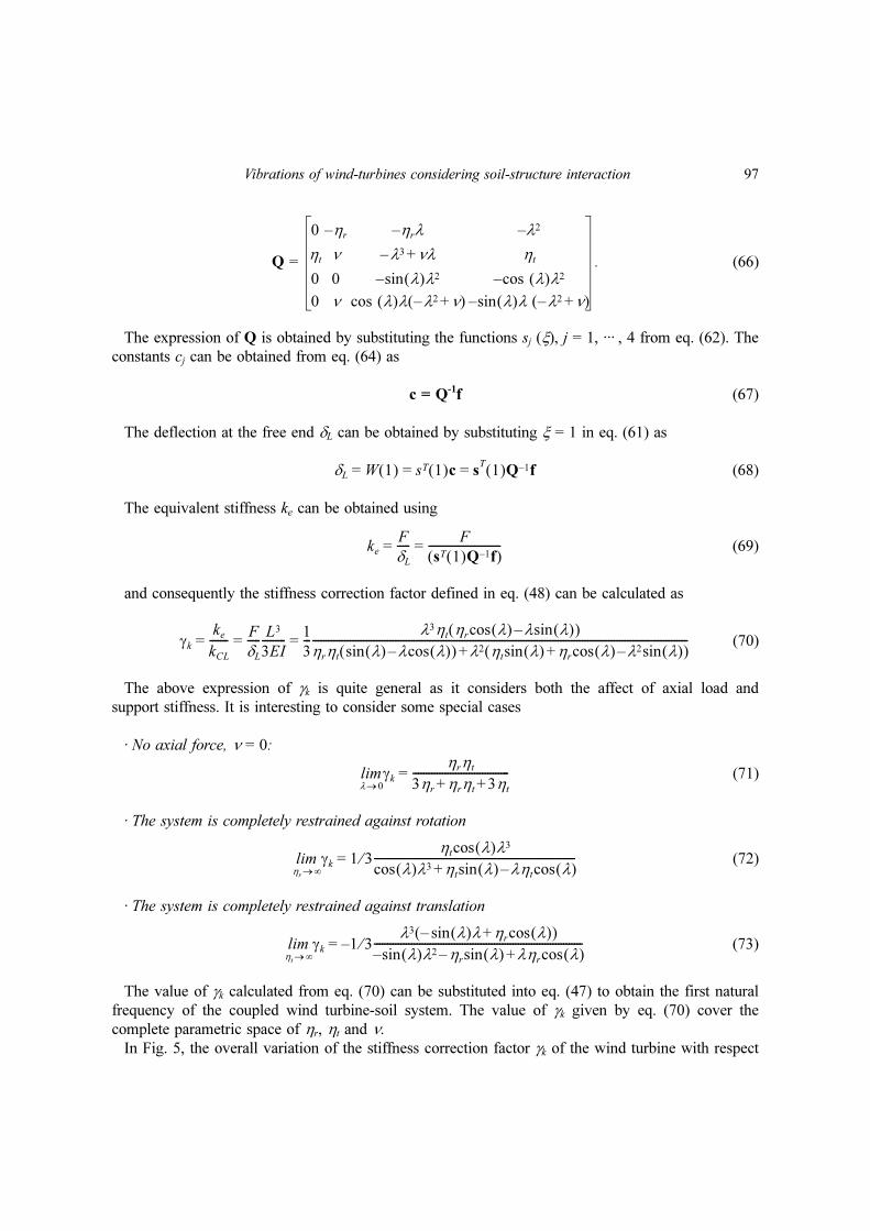
Q = . (66)
The expression of Q is obtained by substituting the functions sj (ξ), j = 1, ··· , 4 from eq. (62). The
constants cj can be obtained from eq. (64) as
c = Q-1
f (67)
The deflection at the free end δL can be obtained by substituting ξ = 1 in eq. (61) as
(68)
The equivalent stiffness ke can be obtained using
(69)
and consequently the stiffness correction factor defined in eq. (48) can be calculated as
(70)
The above expression of γk is quite general as it considers both the affect of axial load and
support stiffness. It is interesting to consider some special cases
· No axial force, ν = 0:
(71)
· The system is completely restrained against rotation
(72)
· The system is completely restrained against translation
(73)
The value of γk calculated from eq. (70) can be substituted into eq. (47) to obtain the first natural
frequency of the coupled wind turbine-soil system. The value of γk given by eq. (70) cover the
complete parametric space of ηr, ηt and ν.
In Fig. 5, the overall variation of the stiffness correction factor γk of the wind turbine with respect
0 ηr– ηr– λ λ2–
ηt ν λ3– νλ+ ηt
0 0 λ( )λ2sin– λ( )λ2cos–
0 ν λ( )λ λ2– ν+( )cos λ( )λ λ2– ν+( )sin–
δL W 1( ) sT 1( )c sT
1( )Q 1– f= = =
ke
F
δL
-----F
sT 1( )Q 1– f( )---------------------------= =
γkke
kCL
-------F
δL
-----L3
3EI---------
1
3---
λ3ηt ηr λ( )cos λ λ( )sin–( )ηrηt λ( )sin λ λ( )cos–( ) λ2 ηt λ( )sin ηr λ( )cos λ2 λ( )sin–+( )+--------------------------------------------------------------------------------------------------------------------------------------------= = =
γkλ 0→
limηrηt
3ηr ηrηt 3ηt+ +------------------------------------=
γkηr
∞→
lim 1 3⁄ηt λ( )λ3cos
λ( )λ3cos ηt λ( )sin ληt λ( )cos–+---------------------------------------------------------------------------=
γkηt
∞→
lim 1– 3⁄λ3 λ( )λsin– ηr λ( )cos+( )λ( )λ2sin ηr λ( )sin ληr λ( )cos+––
------------------------------------------------------------------------------=

98 S. Adhikari and S. Bhattacharya
to both nondimensional rotational soil stiffness and axial load is shown in a 3D plot. Four fixed
values of the nondimensional translational stiffness ηt are considered in the four subplots. The
interesting feature to observe from this plot are (a) the rapid and sharp ‘fall’ in the natural frequency
for small values of ηr and relative flatness for values of ηr approximately over 50, and (b) extremely
high sensitivity for lower values of ν. The parameter ηt has an overall ‘scaling effect’ of the natural
frequency. Higher values of the stiffness corresponds to higher values of the natural frequency as
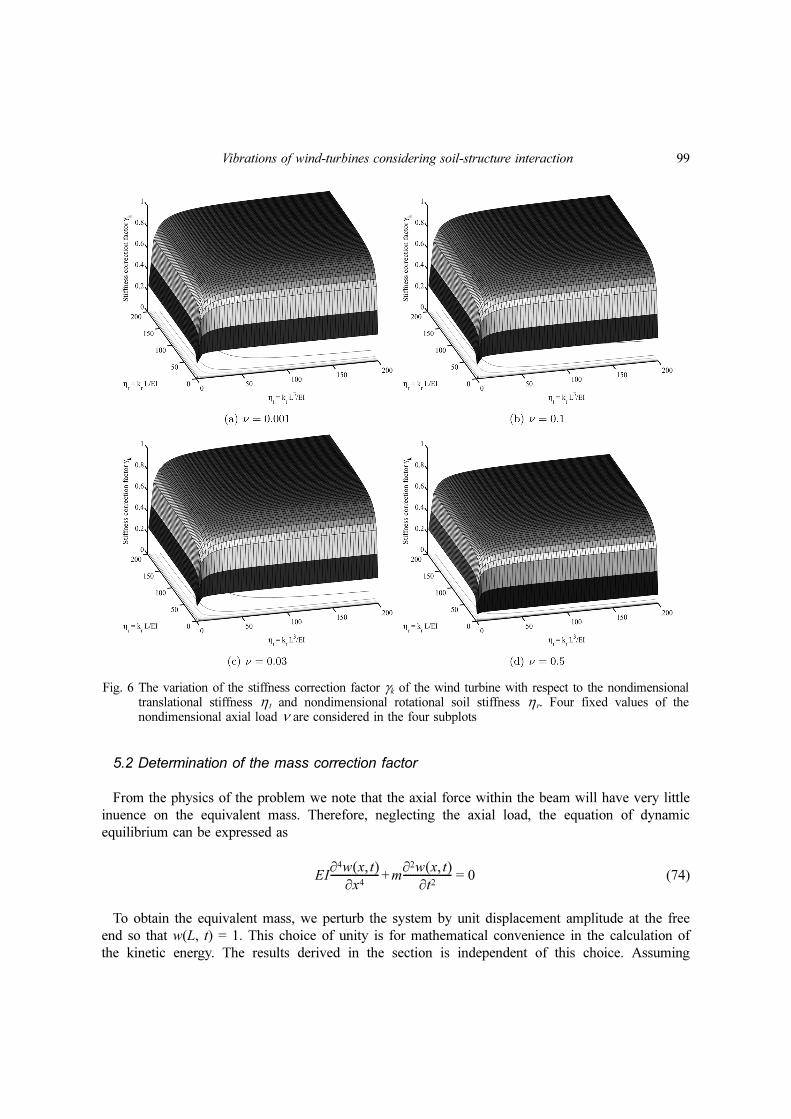
expected. In Fig. 6, the overall variation of the stiffness correction factor γk with respect to both the
nondimensional soil stiffness parameters is shown in a 3D plot. Four fixed values of the
nondimensional axial load ν are considered in the four subplots. It can be seen that lower values of
ν corresponds to higher values of the natural frequency as seen in the previous figures. These plots
can be used to understand the overall design of the system.
Fig. 5 The variation of the stiffness correction factor γk of the wind turbine with respect to the nondimensionalaxial load ν and nondimensional rotational soil stiffness ηr. Four fixed values of the nondimensionaltranslational stiffness η t are considered in the four subplots
Vibrations of wind-turbines considering soil-structure interaction 99
5.2 Determination of the mass correction factor
From the physics of the problem we note that the axial force within the beam will have very little
inuence on the equivalent mass. Therefore, neglecting the axial load, the equation of dynamic
equilibrium can be expressed as
(74)
To obtain the equivalent mass, we perturb the system by unit displacement amplitude at the free
end so that w(L, t) = 1. This choice of unity is for mathematical convenience in the calculation of
the kinetic energy. The results derived in the section is independent of this choice. Assuming
EI∂4w x t,( )
∂x4-------------------- m
∂2w x t,( )∂t2
--------------------+ 0=
Fig. 6 The variation of the stiffness correction factor γk of the wind turbine with respect to the nondimensionaltranslational stiffness η t and nondimensional rotational soil stiffness ηr. Four fixed values of thenondimensional axial load ν are considered in the four subplots
100 S. Adhikari and S. Bhattacharya
standard harmonic solution as in eq. (8), the equation of motion and the four associated boundary
conditions can be expressed as
(75)
(76)
(77)
(78)
W(1) = 1 (79)
We use the static deflection shape as the trial solution. Therefore, W(ξ) can be expressed as
W(ξ) = sT(ξ)c (80)
where the vectors
(81)
and (82)
Applying the boundary conditions in eqs. (76) - (79) on the expression of W(ξ) in (80)
we have
Q c = f (83)
where
(84)
and the matrix
(85)
The expression of Q is obtained by substituting the functions sj (ξ), j = 1, ···, 4 from eq. (81). The
constants cj can be obtained from eq. (83) as
c= Q−1f (86)
d4W ξ( )dξ4
----------------- Ω2W ξ( )– 0=
W '' 0( ) ηrW ' 0( )– 0=
W ''' 0( ) ηtW 0( )+ 0=
W '' 1( ) 0=
s ξ( ) 1 ξ ξ2 ξ3, , , T=
c c1 c2 c3 c4, , , T=
f
0
0
0
1⎩ ⎭⎪ ⎪⎪ ⎪⎨ ⎬⎪ ⎪⎪ ⎪⎧ ⎫
=
Q
0 ηr– 2 0
ηt 0 0 6
0 0 2 6
1 1 1 1
=

Vibrations of wind-turbines considering soil-structure interaction 101
Considering harmonic motion as in eq. (8), the kinetic energy of the beam can be obtained as
(87)
where the mass correction factor is given by
(88)
Evaluating this integral we have
(89)
In Fig. 7 the parametric variation of of the mass correction factor γm of a cantilever wind turbine
with respect to both the nondimensional soil stiffness parameters is shown in a 3D plot. It is
interesting to consider the special case when the support is completely restrained. Taking the
limit and we have
Tω
2
2------ mW2 x( ) xd
ω2
2------MW2 L( )+
0
L
∫=
mLω
2
2------ WT ξ( )W ξ( ) ξd
0
1
∫ω
2
2------M12+=
mLω
2
2------ cTs ξ( )sT ξ( )c ξd
0
1
∫ω
2
2------M+=
ω2
2------ mLγm M+( )=
γm cTs ξ( )sT ξ( )c ξd0
1
∫=
γm3
140---------
11ηr
2ηt
277ηt
2ηr 105ηr
2ηt 140ηt
2420ηrηt 420ηr
2+ + + + +
9ηr
26ηr
2ηt 18ηrηt ηr
2ηt
26ηt
2ηr 9ηt
2+ + + + +
----------------------------------------------------------------------------------------------------------------------------------------=
ηr ∞→ ηt ∞→
Fig. 7 The variation of the mass correction factor γm of the wind turbine with respect to the nondimensionaltranslational stiffness η t and nondimensional rotational soil stiffness ηr.
102 S. Adhikari and S. Bhattacharya
(90)
which agrees exactly with Table 8-8, case 1, page 158 of Blevins (1984). This analysis shows that
the expression of γm is the generalization of the classical case so that it considerers the effect of
elastic foundation.
6. Validation and practical applications of the proposed approach
6.1 Numerical validation
In this section we aim to validate the approximate expressions developed against the exact results.
First we determine the relevant non-dimensional parameters in the equations derived here. We focus
our attention on the affect of ν and the non-dimensional foundation rotational stiffness ηr on the
first-natural frequency. For this reason, the numerical results are presented as a function of ν and ηr.
These two parameters are considered because the boundary condition and the load of the turbine are
the crucial design issues for the overall system.
The non-dimensional mass ratio can be obtained as
(91)
We consider the rotary inertia of the blade assembly J = 0. This is not a very bad assumption if
there is very less misalignment.
In this example we have used the data of a wind turbine given by Tempel and Molenaar (2002).
The numerical values of the main parameters are summarised in Table 1. The moment of inertia of
the circular cross section can be obtained as
(92)
γmηr
∞→ ηt
∞→,
lim33
140--------- 0.2357= =
α M
mL-------
P
gmL-----------
PL2
EI---------
EI
gmL3-------------⎝ ⎠⎛ ⎞ ν
EI
mL4---------⎝ ⎠⎛ ⎞L g⁄ νc0
2L g⁄= = = = =
Iπ
64------D4
π
64------ D th–( )4 1
16------πD
3th≈– 0.6314m4= =
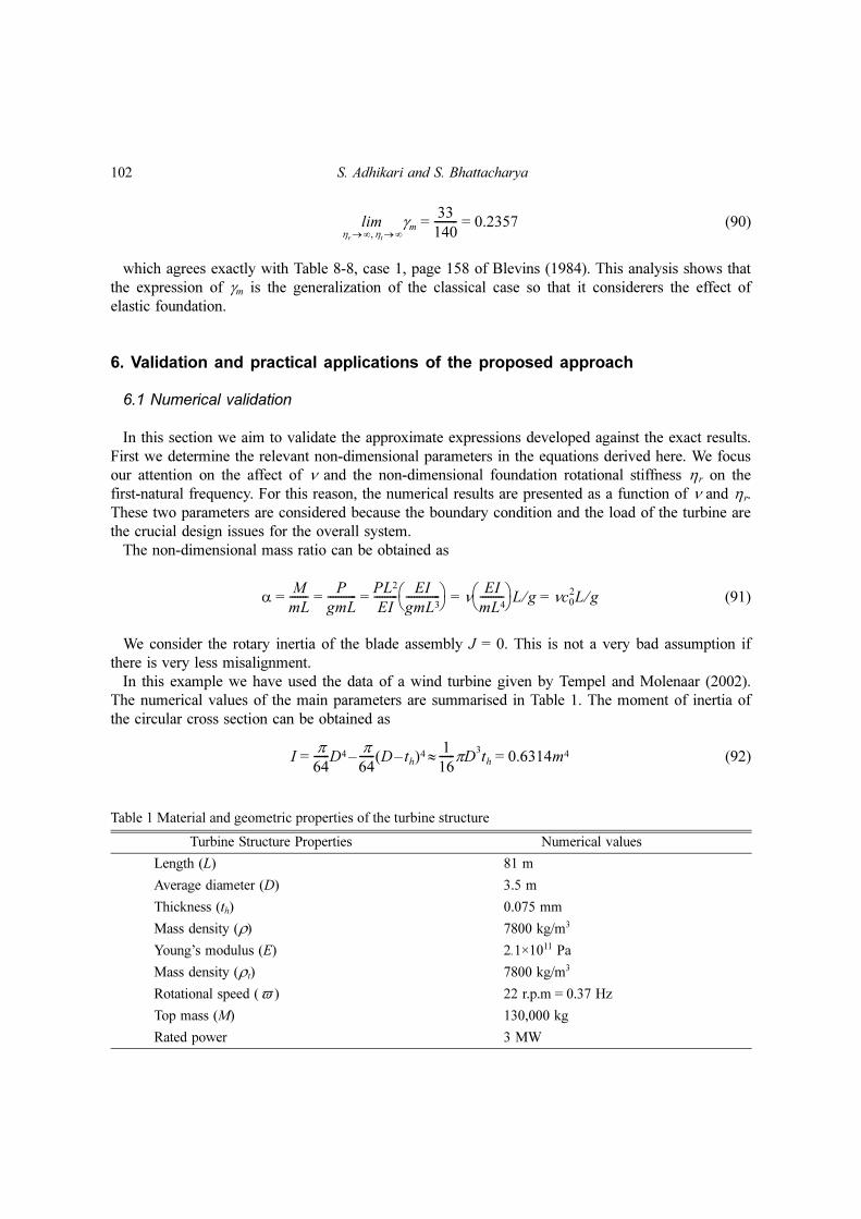
Table 1 Material and geometric properties of the turbine structure
Turbine Structure Properties Numerical values
Length (L) 81 m
Average diameter (D) 3.5 m
Thickness (th) 0.075 mm
Mass density (ρ) 7800 kg/m3
Young’s modulus (E) 2.1×10¹¹ Pa
Mass density (ρt) 7800 kg/m3
Rotational speed ( ) 22 r.p.m = 0.37 Hz
Top mass (M) 130,000 kg
Rated power 3 MW
ϖ
Vibrations of wind-turbines considering soil-structure interaction 103
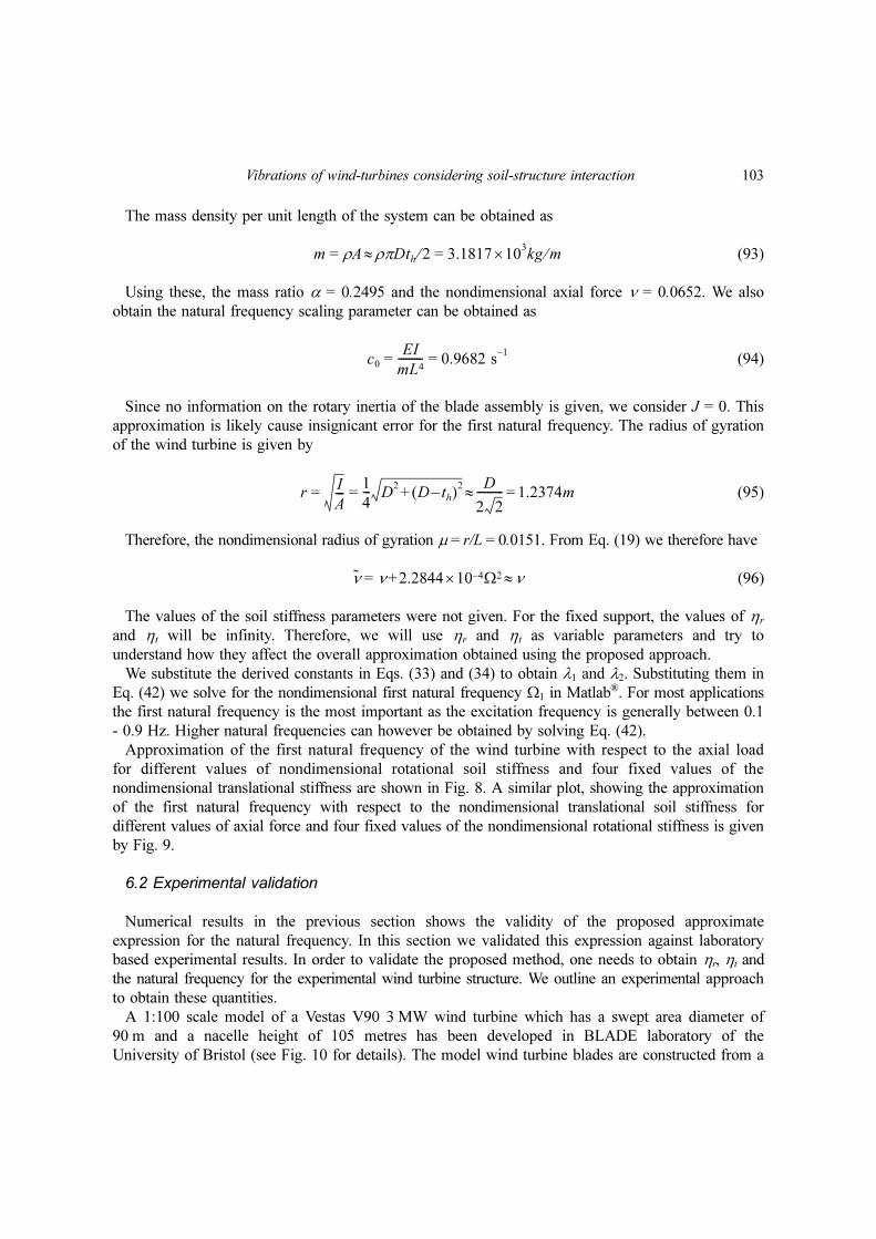
The mass density per unit length of the system can be obtained as
(93)
Using these, the mass ratio α = 0.2495 and the nondimensional axial force ν = 0.0652. We also
obtain the natural frequency scaling parameter can be obtained as
(94)
Since no information on the rotary inertia of the blade assembly is given, we consider J = 0. This
approximation is likely cause insignicant error for the first natural frequency. The radius of gyration
of the wind turbine is given by
(95)
Therefore, the nondimensional radius of gyration µ = r/L = 0.0151. From Eq. (19) we therefore have
(96)
The values of the soil stiffness parameters were not given. For the fixed support, the values of ηr
and ηt will be infinity. Therefore, we will use ηr and ηt as variable parameters and try to
understand how they affect the overall approximation obtained using the proposed approach.
We substitute the derived constants in Eqs. (33) and (34) to obtain λ1 and λ2. Substituting them in
Eq. (42) we solve for the nondimensional first natural frequency Ω1 in Matlab®. For most applications
the first natural frequency is the most important as the excitation frequency is generally between 0.1
- 0.9 Hz. Higher natural frequencies can however be obtained by solving Eq. (42).
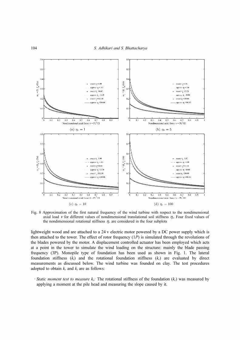
Approximation of the first natural frequency of the wind turbine with respect to the axial load
for different values of nondimensional rotational soil stiffness and four fixed values of the
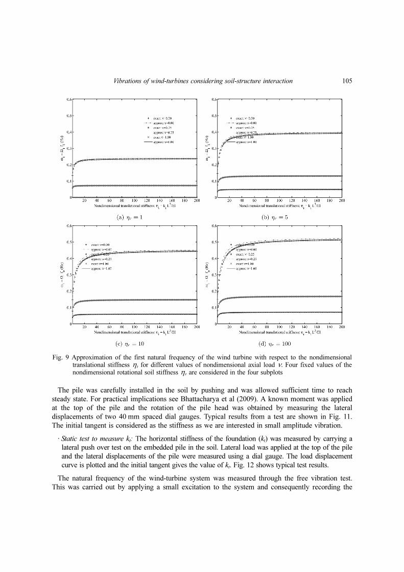
nondimensional translational stiffness are shown in Fig. 8. A similar plot, showing the approximation
of the first natural frequency with respect to the nondimensional translational soil stiffness for
different values of axial force and four fixed values of the nondimensional rotational stiffness is given
by Fig. 9.
6.2 Experimental validation
Numerical results in the previous section shows the validity of the proposed approximate
expression for the natural frequency. In this section we validated this expression against laboratory
based experimental results. In order to validate the proposed method, one needs to obtain ηr, ηt and
the natural frequency for the experimental wind turbine structure. We outline an experimental approach
to obtain these quantities.
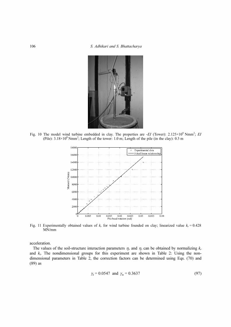
A 1:100 scale model of a Vestas V90 3 MW wind turbine which has a swept area diameter of
90 m and a nacelle height of 105 metres has been developed in BLADE laboratory of the
University of Bristol (see Fig. 10 for details). The model wind turbine blades are constructed from a
m ρA ρπDth 2⁄≈ 3.1817 103kg m⁄×= =
c0
EI
mL4--------- 0.9682 s
1–= =
rI
A---
1
4--- D
2D th–( )2+
D
2 2---------- 1.2374m=≈= =
ν ν 2.2844 10 4– Ω2 ν≈×+=
104 S. Adhikari and S. Bhattacharya
lightweight wood and are attached to a 24 v electric motor powered by a DC power supply which is
then attached to the tower. The effect of rotor frequency (1P) is simulated through the revolutions of
the blades powered by the motor. A displacement controlled actuator has been employed which acts
at a point in the tower to simulate the wind loading on the structure: mainly the blade passing
frequency (3P). Monopile type of foundation has been used as shown in Fig. 1. The lateral
foundation stiffness (kt) and the rotational foundation stiffness (kr) are evaluated by direct
measurements as discussed below. The wind turbine was founded on clay. The test procedures
adopted to obtain kr and kt are as follows:
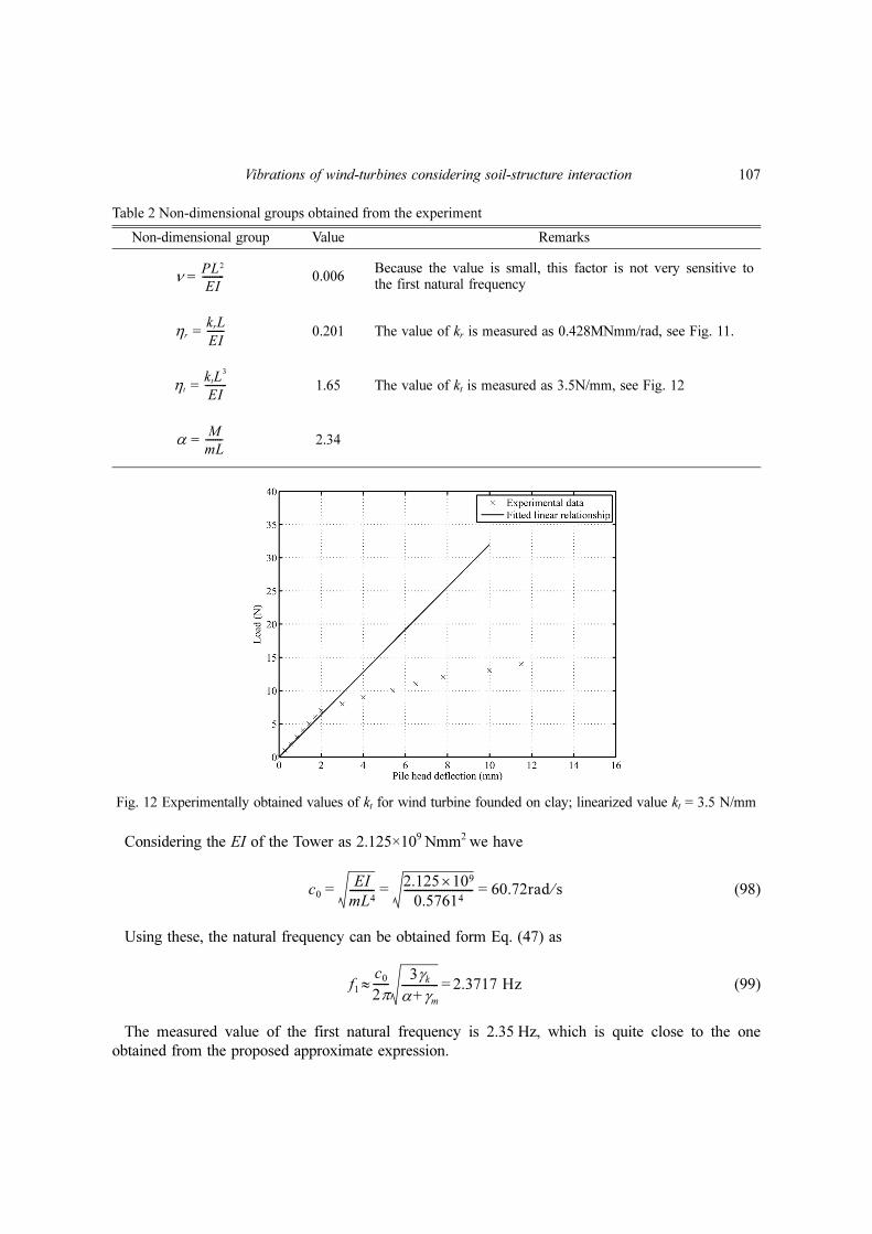
· Static moment test to measure kr: The rotational stiffness of the foundation (kr) was measured by
applying a moment at the pile head and measuring the slope caused by it.
Fig. 8 Approximation of the first natural frequency of the wind turbine with respect to the nondimensionalaxial load ν for different values of nondimensional translational soil stiffness ηt. Four fixed values ofthe nondimensional rotational stiffness ηr are considered in the four subplots
Vibrations of wind-turbines considering soil-structure interaction 105
The pile was carefully installed in the soil by pushing and was allowed sufficient time to reach
steady state. For practical implications see Bhattacharya et al (2009). A known moment was applied
at the top of the pile and the rotation of the pile head was obtained by measuring the lateral
displacements of two 40 mm spaced dial gauges. Typical results from a test are shown in Fig. 11.
The initial tangent is considered as the stiffness as we are interested in small amplitude vibration.
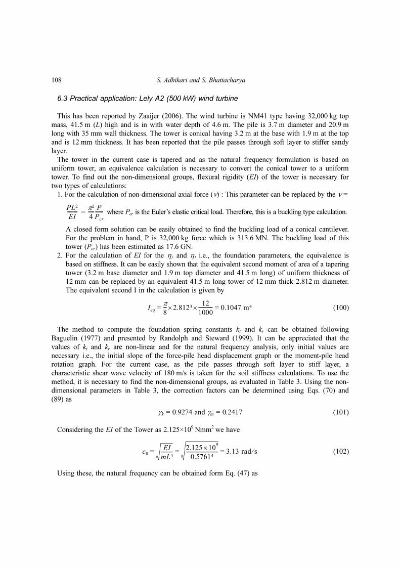
· Static test to measure kt: The horizontal stiffness of the foundation (kt) was measured by carrying a
lateral push over test on the embedded pile in the soil. Lateral load was applied at the top of the pile
and the lateral displacements of the pile were measured using a dial gauge. The load displacement
curve is plotted and the initial tangent gives the value of kt. Fig. 12 shows typical test results.
The natural frequency of the wind-turbine system was measured through the free vibration test.
This was carried out by applying a small excitation to the system and consequently recording the
Fig. 9 Approximation of the first natural frequency of the wind turbine with respect to the nondimensionaltranslational stiffness ηt for different values of nondimensional axial load ν. Four fixed values of thenondimensional rotational soil stiffness ηr are considered in the four subplots
106 S. Adhikari and S. Bhattacharya
acceleration.
The values of the soil-structure interaction parameters ηr and ηt can be obtained by normalizing krand kt. The nondimensional groups for this experiment are shown in Table 2: Using the non-
dimensional parameters in Table 2, the correction factors can be determined using Eqs. (70) and
(89) as
and (97)γk 0.0547= γm 0.3637=
Fig. 10 The model wind turbine embedded in clay. The properties are -EI (Tower): 2.125×10⁹ Nmm2; EI(Pile): 3.18×10⁸ Nmm2; Length of the tower: 1.0 m; Length of the pile (in the clay): 0.5 m
Fig. 11 Experimentally obtained values of kr for wind turbine founded on clay; linearized value kr = 0.428MN/mm
Vibrations of wind-turbines considering soil-structure interaction 107
Considering the EI of the Tower as 2.125×10⁹ Nmm2 we have
(98)
Using these, the natural frequency can be obtained form Eq. (47) as
(99)
The measured value of the first natural frequency is 2.35 Hz, which is quite close to the one
obtained from the proposed approximate expression.
c0
EI
mL4---------
2.125 109×0.57614
-------------------------- 60.72rad s⁄= = =
f1c0
2π------
3γkα γm+-------------- 2.3717 Hz=≈
Table 2 Non-dimensional groups obtained from the experiment
Non-dimensional group Value Remarks
ν = 0.006 Because the value is small, this factor is not very sensitive tothe first natural frequency
0.201 The value of kr is measured as 0.428MNmm/rad, see Fig. 11.
1.65 The value of kt is measured as 3.5N/mm, see Fig. 12
2.34
PL2
EI---------
ηr
krL
EI-------=
ηt
ktL3
EI---------=
αM
mL-------=
Fig. 12 Experimentally obtained values of kt for wind turbine founded on clay; linearized value kt = 3.5 N/mm
108 S. Adhikari and S. Bhattacharya
6.3 Practical application: Lely A2 (500 kW) wind turbine
This has been reported by Zaaijer (2006). The wind turbine is NM41 type having 32,000 kg top
mass, 41.5 m (L) high and is in with water depth of 4.6 m. The pile is 3.7 m diameter and 20.9 m
long with 35 mm wall thickness. The tower is conical having 3.2 m at the base with 1.9 m at the top
and is 12 mm thickness. It has been reported that the pile passes through soft layer to stiffer sandy
layer.
The tower in the current case is tapered and as the natural frequency formulation is based on
uniform tower, an equivalence calculation is necessary to convert the conical tower to a uniform
tower. To find out the non-dimensional groups, flexural rigidity (EI) of the tower is necessary for
two types of calculations:
1. For the calculation of non-dimensional axial force (ν) : This parameter can be replaced by the ν =
= where Pcr is the Euler’s elastic critical load. Therefore, this is a buckling type calculation.
A closed form solution can be easily obtained to find the buckling load of a conical cantilever.
For the problem in hand, P is 32,000 kg force which is 313.6 MN. The buckling load of this
tower (Pcr) has been estimated as 17.6 GN.
2. For the calculation of EI for the ηr and ηt i.e., the foundation parameters, the equivalence is
based on stiffness. It can be easily shown that the equivalent second moment of area of a tapering
tower (3.2 m base diameter and 1.9 m top diameter and 41.5 m long) of uniform thickness of
12 mm can be replaced by an equivalent 41.5 m long tower of 12 mm thick 2.812 m diameter.
The equivalent second I in the calculation is given by
(100)
The method to compute the foundation spring constants kt and kr can be obtained following
Baguelin (1977) and presented by Randolph and Steward (1999). It can be appreciated that the
values of kt and kr are non-linear and for the natural frequency analysis, only initial values are
necessary i.e., the initial slope of the force-pile head displacement graph or the moment-pile head
rotation graph. For the current case, as the pile passes through soft layer to stiff layer, a
characteristic shear wave velocity of 180 m/s is taken for the soil stiffness calculations. To use the
method, it is necessary to find the non-dimensional groups, as evaluated in Table 3. Using the non-
dimensional parameters in Table 3, the correction factors can be determined using Eqs. (70) and
(89) as
γk = 0.9274 and γm = 0.2417 (101)
Considering the EI of the Tower as 2.125×10⁹ Nmm2 we have
(102)
Using these, the natural frequency can be obtained form Eq. (47) as
PL2
EI---------
π2
4-----
P
Pcr
-------
Ieqπ
8--- 2.8123×
12
1000------------× 0.1047 m4= =
c0
EI
mL4---------
2.125 109×
0.57614-------------------------- 3.13 rad s⁄= = =
Vibrations of wind-turbines considering soil-structure interaction 109
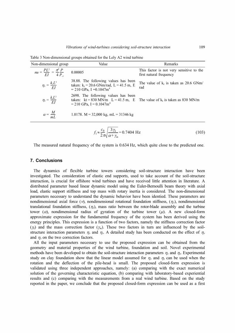
(103)
The measured natural frequency of the system is 0.634 Hz, which quite close to the predicted one.
7. Conclusions
The dynamics of flexible turbine towers considering soil-structure interaction have been
investigated. The consideration of elastic end supports, used to take account of the soil-structure
interaction, is crucial for offshore wind turbines and have received little attention in literature. A
distributed parameter based linear dynamic model using the Euler-Bernoulli beam theory with axial
load, elastic support stiffness and top mass with rotary inertia is considered. The non-dimensional
parameters necessary to understand the dynamic behavior have been identied. These parameters are
nondimensional axial force (ν), nondimensional rotational foundation stiffness, (ηr), nondimensional
translational foundation stiffness, (ηt), mass ratio between the rotor-blade assembly and the turbine
tower (α), nondimensional radius of gyration of the turbine tower (µ). A new closed-form
approximate expression for the fundamental frequency of the system has been derived using the
energy principles. This expression is a function of two factors, namely the stiffness correction factor
(γk) and the mass correction factor (γm). These two factors in turn are influenced by the soil-
structure interaction parameters ηr and ηt. A detailed study has been conducted on the effect of ηr
and ηt on the two correction factors.
All the input parameters necessary to use the proposed expression can be obtained from the
geometry and material properties of the wind turbine, foundation and soil. Novel experimental
methods have been developed to obtain the soil-structure interaction parameters ηr and ηt. Experimental
study on clay foundation show that the linear model assumed for ηr and ηt can be used when the
rotation and the deflection of the pile-head is small. The proposed closed-form expression is
validated using three independent approaches, namely: (a) comparing with the exact numerical
solution of the governing characteristic equation, (b) comparing with laboratory-based experiential
results and (c) comparing with the measurements from a real wind turbine. Based on the study
reported in the paper, we conclude that the proposed closed-form expression can be used as a first
f1c0
2π------
3γkα γm+-------------- 0.7404 Hz=≈
Table 3 Non-dimensional groups obtained for the Lely A2 wind turbine
Non-dimensional group Value Remarks
nu = = 0.00005 This factor is not very sensitive to thefirst natural frequency
ηr = 38.88. The following values has beentaken: kr = 20.6 GNm/rad, L = 41.5 m, E= 210 GPa, I =0.1047m4
The value of kr is taken as 20.6 GNm/rad
ηt = 2698. The following values has beentaken: kt = 830 MN/m L = 41.5 m, E= 210 GPa, I = 0.1047m4
The value of kt is taken as 830 MN/m
α = 1.0178. M = 32,000 kg, mL = 31346 kg
PL2
EI---------
π2
4-----
P
Pcr
------
krL3
EI---------
ktL3
EI---------
M
mL-------
110 S. Adhikari and S. Bhattacharya
step to obtain the fundamental frequency of wind turbine towers considering the soil-structure
interaction into account.
Acknowledgments
SA gratefully acknowledges the support of The Leverhulme Trust for the award of the Philip
Leverhulme Prize.
References
Abramovich, H. and Hamburger, O. (1991), “Vibration of a cantilever timoshenko beam with a tip mass”, J.Sound Vib.,148(1), 162-170.
Adhikari, S. (1999a), “Modal analysis of linear asymmetric non-conservative systems”, J. Eng. Mech.- ASCE.,125(12), 1372-1379.
Adhikari, S. (1999b), “Rates of change of eigenvalues and eigenvectors in damped dynamic systems”, J. AIAA,37(11), 1452-1458.
Adhikari, S. (2004), “Optimal complex modes and an index of damping non-proportionality”, Mech. Syst. SignalPr.,18(1), 1-27.
Adhikari, S. and Bhattacharya, S. (2008), “Dynamic instability of pile-supported structures in liquefiable soilsduring earthquakes”, Shock Vib., 15(6), 665-685.
Adhikari, S. and Bhattacharya, S. (2011), “Dynamic analysis of wind turbine towers on flexible foundations”,Shock Vib.
Baguelin F., Frank R., S. Y. (1977), “Theoretical study of lateral reaction mechanism of piles”, Géotechnique, 27,405-434.
Bhattacharya, S., Adhikari, S. and Alexander, N. A. (2009), “A simplied method for unied buckling and dynamicanalysis of pile-supported structures in seismically liquefiable soils”, Soil Dyn. Earthq. Eng., 29(8), 1220-1235.
Bhattacharya, S., Carrington, T. and Aldridge, T. (2009), “Observed increases in offshore pile driving resistance”,Proceedings of the Institution of Civil Engineers-Geotechnical Engineering, 162(1), 71-80.
Bhattacharya, S., Dash, S.R. and Adhikari, S. (2008), “On the mechanics of failure of pile-supported structures inliqueable deposits during earthquakes”, Current Science, 94(5), 605-611.
Blevins, R.D. (1984), Formulas for Natural Frequency and Mode Shape, Krieger Publishing Company, Malabar,FL, USA.
Byrne, B. and Houlsby, G. (2003), “Foundations for offshore wind turbine”, Philos. T. R. Soc. A., 361.Chen, Y. (1963), “On the vibration of beams or rods carrying a concentrated mass”, J. Appl. Mech –T. ASME.,
30, 310-311.Dash, S.R., Govindaraju, L. and Bhattacharya, S. (2009), “A case study of damages of the Kandla Port and
Customs Office tower supported on a mat-pile foundation in liquefied soils under the 2001 Bhuj earthquake”,Soil Dyn. Earthq. Eng., 29(2), 333-346.
DnV (2001), Guidelines for design of wind turbines-DnV/Riso, Code of practice, DnV, USA.Elishakoff, I. and Johnson, V. (2005), “Apparently the first closed-form solution of vibrating inhomogeneous
beam with a tip mass”, J. Sound Vib., 286(4-5), 1057-1066.Elishakoff, I. and Perez, A. (2005), “Design of a polynomially inhomogeneous bar with a tip mass for specied
mode shape and natural frequency”, J. Sound Vib., 287(4-5), 1004-1012.GHBLADED (2009), Wind Turbine Design Software, Garrad Hassan Limited, Bristol, UK.Gurgoze, M. (2005a), “On the eigenfrequencies of a cantilever beam carrying a tip spring-mass system with
mass of the helical spring considered, J. Sound Vib., 282(3-5), 1221-1230.Gurgoze, M. (2005b), “On the representation of a cantilevered beam carrying a tip mass by an equivalent
Vibrations of wind-turbines considering soil-structure interaction 111
springmass system”, J. Sound Vib., 282, 538-542.Gurgoze, M. and Erol, H. (2002), “On the frequency response function of a damped cantilever simply supported
in-span and carrying a tip mass”, J. Sound Vib., 255(3), 489-500.Hetenyi, M. (1946), “Beams on Elastic Foundation: Theory with Applications in the Fields of Civil and
Mechanical Engineering”, University of Michigan Press, Ann Arbor, MI USA.Huang, T.C. (1961), “The effect of rotatory inertia and of shear deformation on the frequency and normal mode
equations of uniform beams with simple end conditions”, J. Appl. Mech – T. ASME., 28, 579-584.IEA (2005), International Energy Statistics 2005: Key World Energy Statistics, International Energy Agency,
Paris, France.Kreyszig, E. (2006), Advanced engineering mathematics, 9th Edition., John Wiley & Sons, New York.Laura, P.A.A. and Gutierrez, R.H. (1986), “Vibrations of an elastically restrained cantilever beam of varying
cross-section with tip mass of finite length”, J. Sound Vib., 108(1), 123-131.Oz, H.R. (2003), “Natural frequencies of an immersed beam carrying a tip mass with rotatory inertia”, J. Sound
Vib., 266(5), 1099-1108.Randolph, M.F. and Steward, D.P. (1999), Manual for the program PYGM , University of Western Australia,
Australia.SAMTECH (2009), SAMCEF for Wind Turbine (S4WT), SAMTECT s.a., Liege, Belgium.Sheu, G. and Yang, S. (2005), “Dynamic analysis of a spinning rayleigh beam”, Int. J. Mech. Sci., 47(2), 157-
169.Tempel, D.P. and Molenaar, D.P. (2002), “Wind turbine structural dynamics -a review of the principles for
modern power generation, onshore and offshore”, Wind Eng., 26(4), 211-220.Wu, J.S. and Chou, H.M. (1998), “Free vibration analysis of a cantilever beam carrying any number of
elastically mounted point masses with the analytical-and-numerical-combined method”, J. Sound Vib., 213(2),317-332.
Wu, J.S. and Chou, H.M. (1999), “A new approach for determining the natural frequencies and mode shapes ofa uniform beam carrying any number of sprung masses”, J. Sound Vib., 220(3), 451- 468.
Wu, J.S. and Hsu, S.H. (2006), “A unified approach for the free vibration analysis of an elastically supportedimmersed uniform beam carrying an eccentric tip mass with rotary inertia”, J. Sound Vib., 291(3-5), 1122-1147.
Zaaijer, M. (2006), “Foundation modelling to assess dynamic behaviour of offshore wind turbines”, Appl. OceanRes., 28, 45-57.
CC
Nomenclature
α mass ratio, α =
β nondimensional rotary inertia, β =
ηr nondimensional rotational end stiffness, ηr =
η t nondimensional translational end stiffness, η t =
γk stiffness correction factor, γk =
γm mass correction factor
µ nondimensional radius of gyration, µ =
M
mL-------
J
mL3---------
krL
EI-------
krL3
EI---------
ke
kCL
-------
r
L---

112 S. Adhikari and S. Bhattacharya
ν nondimensional axial force, ν =
Ω nondimensional frequency parameter, Ω2 = ω2
ω angular frequency (rad/s)
ξ non-dimensional length parameter, ξ = x/L
c0 natural frequency scaling parameter (s-1), c0 =
EI bending stiffness of the beam
F(ξ) transverse force on the beam
f(x, t) applied time dependent distributed load on the beam
fi natural frequency (Hz)
J rotary inertia of the rotor system
ke equivalent end stiffness of the beam
kr rotational end stiffness of the elastic support
kt translational (linear) end stiffness of the elastic support
kCL equivalent end stiffness of a cantilever beam, kCL =
L length of the beam
M mass of the rotor system
m mass per unit length of the beam, m = ρA
Mb mass of the beam, Mb = mL
Me equivalent mass of the SDOF system
P constant axial force in the beam
r radius of gyration of the beam
t time
W(ξ) transverse deflection of the beam
w(x, t) time depended transverse deflection of the beam
x spatial coordinate along the length of the beam
( ) derivative with respect to the spatial coordinate
( )T matrix transposition
( ) derivative with respect to time
( ) determinant of a matrix
PL2
EI---------
mL4
EI---------
EI
mL4---------
3EI
L3---------
•'••·
•