1

Vibrational characteristics of a piled structure in liquefied soil during earthquakes: Experimental Investigation (Part I) and Analytical Modelling (Part II)

by

Subhamoy Bhattacharya1 Sondipon Adhikari2

Report No. OUEL 2294 / 07

University of Oxford, Department of Engineering Science, Parks Road, Oxford, OX1 3PJ, U.K.

Tel. 01865 273162/283300 Fax. 01865 283301

Email: civil@eng.ox.ac.uk http://www-civil.eng.ox.ac.uk/

1 Departmental Lecturer, Department of Engineering Science, Oxford University 2 EPSRC Advanced Research Fellow and Lecturer in Aerospace Engineering, Bristol University

2

Vibrational characteristics of a piled structure in liquefied soil during earthquakes: Part 1 (Experimental Investigation)

Subhamoy Bhattacharya and Sondipon Adhikari

ABSTRACT The collapse of pile-supported structures is still observed in liquefiable soils after most major earthquakes causing great concerns to the earthquake geotechnical engineers. A safe design approach would require the foundation to vibrate in the liquefied soil without exceeding yield anywhere in the pile. The forcing function for these vibrations is predominantly due to the inertia of the superstructure. This paper and its companion are aimed at modelling the dynamics of pile in liquefiable soils during earthquakes. Two aspects of vibration are considered: (a) Variation of the first natural frequency of the piled foundations as the surrounding soil liquefies; (b) Damping provided by the liquefied soil to the vibrating pile. This paper analyses high quality experimental data obtained from dynamic centrifuge tests to characterise these aspects of vibration. The experimental system consists of a cantilever column with a tip mass embedded in a soil which was subsequently liquefied. A Single Degree of Freedom (SDOF) model has been fitted to the measured data using two approaches. The first approach is based on simplified graphical analysis based on classical understanding of vibration. The second approach is based on a nonlinear least-square error minimisation method. The results obtained from the two approaches are compared and conclusions are drawn. Keywords: Vibration, Failure, Pile, SDOF, Damping, Centrifuge INTRODUCTION Collapse and/or severe damage of pile-supported structures is still observed in liquefiable soils after most major earthquakes such as the 1995 Kobe earthquake (JAPAN), the 1999 Kocheli earthquake (TURKEY), and the 2001 Bhuj earthquake (INDIA). The failures not only occurred in laterally spreading (sloping) ground but were also observed in level ground where no lateral spreading would be anticipated; see for example Tokimatsu and Asaka (1998). The failures were often accompanied by settlement and tilting of the superstructure, rendering it either useless or very expensive to rehabilitate after the earthquake. Following the 1995 Kobe earthquake, investigations has been carried out to find the failure pattern of the piles; see Yoshida and Hamada (1990), BTL (2000). Piles were excavated or extracted from the subsoil, borehole cameras were used to take photographs, and pile integrity tests were carried out. These studies hinted the location of the cracks and damage patterns for the piles. Of particular interest is the formation of plastic hinges in the piles. This indicates that the stresses in the pile during and after liquefaction exceeded the yield stress of the material of the pile, despite large factors of safety were employed in the design. As a result, design of pile foundation in seismically liquefiable areas still remains a continuing area of concern for the earthquake geotechnical engineering community. There are two competing theories regarding the cause of failure of piled foundations in liquefiable soils, see Bhattacharya et al (2005a). One of the theories is based on a bending mechanism where the lateral loads due to inertia and lateral spreading induce bending failure in the pile; see for example JRA (2002), Abdoun and Dobry (2002), Ishihara (1997), Hamada (1992). The down-slope deformation of the ground surface adjacent to the piled foundation seems to support this explanation. This theory therefore assumes piles as laterally loaded beams. The other theory, which is relatively new, is based on buckling instability; see Bhattacharya and Bolton (2004), Bhattacharya et al (2004), Knappett and Madabhushi (2005). This theory treats the piles as

3

laterally unsupported slender columns in liquefied zone and therefore prone to buckling instability (bifurcation). Bhattacharya et al (2005b) have demonstrated that the theory of pile failure based on bending cannot explain various observations of pile failure. They have shown that while the design of the Showa Bridge piles satisfies the latest version of JRA (1996 or 2002), the bridge actually collapsed during the 1964 Niigata earthquake. They have also shown that the bridge foundations are unsafe against buckling instability which can be plausible cause of the collapse. Figure 1 shows the collapse of a building supported on 38 piles. The building was located 6m from the quay wall on a reclaimed land in Higashinada-ku area of Kobe City. After the 1995 Kobe earthquake, the quay wall was displaced by 2m towards the sea and the building tilted by about 3 degrees. Following the earthquake, investigation was carried out to find the damage pattern, see Figure 2. Figure 3 shows the foundation plan along with the location of the piles for the building shown in Figure 1. The failure pattern suggests that the building supported on the piles rotated during the earthquake. This type of observation has also been observed in carefully designed small scale model tests carried out by Bhattacharya et al (2004), Knappett and Madabhushi (2005) while studying the buckling instability of piled foundations in liquefiable soils. Figures 4 (a & b) show the failure pattern of a single pile and a pile group observed in a centrifuge test. This implies that the rotary inertia of the building mass (i.e. mass moment of inertia of the rigid body) should be considered in the analysis. One of the aims of this paper and its companion is to investigate the effects of the rotary inertia of the building mass towards the cause of failure of pile-supported structures during seismic liquefaction. The next section describes the different phases of loading in a piled foundation that need consideration while analysing/ designing them.

Figure 1: Failure of a pile-supported building during 1995 Kobe earthquake

4

Figure 2: Failure pattern of the piles for the building shown in Figure 1

Figure 3: Foundation arrangement of the piles for the building in Figure 1

Figure 4: Instability of piled foundations observed in centrifuge tests; (a) A single pile; (b) A pile group, Knappett and Madabhushi (2005).

5

DIFFERENT PHASES OF LOADING IN A PILE DURING EARTHQUAKE LIQUEFACTION Before Liquefaction Figure 5 shows the different stages of loading on a pile-supported foundation during an earthquake. Stage I in the figure describes the load sharing between the shaft resistance and end-bearing of the pile in normal condition i.e. prior to an earthquake. The vertical load of the building which can be considered purely static (Pstatic) is carried by the shear generated along the length of the pile and end-bearing of the pile. However, during earthquakes, soil layers overlying the bedrock are subjected to seismic excitation consisting of numerous incident waves, namely shear (S) waves, dilatational or pressure (P) waves, and surface (Rayleigh and Love) waves, all of which result in ground motion. The ground motion at a site will depend on the stiffness characteristics of the layers of soil overlying the bedrock. This motion will also affect a piled structure. As the seismic waves arrive in the soil surrounding the pile, the soil layers will tend to deform. This seismically deforming soil will try to move the piles and the embedded pile-cap with it. Subsequently, depending upon the rigidity of the superstructure and the pile-cap, the superstructure may also move with the foundation. The pile may thus experience two distinct phases of initial soil-structure interaction.

1) Before the superstructure starts oscillating, the piles may be forced to follow the soil motion, depending on the flexural rigidity (EI) of the pile. Here the soil and pile may take part in kinematic interplay and the motion of the pile may differ substantially from the free field motion. This may induce bending moments in the pile.

2) As the superstructure starts to oscillate, inertial forces are generated. These inertia forces are transferred as lateral forces and overturning moments to the pile via the pile-cap. The pile-cap transfers the moments as varying axial loads and bending moments in the piles. Thus the piles may experience additional axial (Pdynamic) and lateral loads (Plateral), which cause additional bending moments in the pile.

These two effects occur with only a small time lag. If the section of the pile is inadequate, bending failure may occur in the pile. The behaviour of the pile at this stage may be approximately described as a beam on an elastic foundation, where the soil provides sufficient lateral restraint. The available confining pressure around the pile is not expected to decrease substantially in these initial phases. The response to changes in axial load in the pile would not be severe either, as shaft resistance continues to act. This is shown in Figure 5 (Stage II). After Liquefaction In loose saturated sandy soil, as the shaking continues, pore pressure will build up and the soil will start to liquefy. With the onset of liquefaction, an end-bearing pile passing through liquefiable soil will experience distinct changes in its stress state.

• The pile will start to lose its shaft resistance in the liquefied layer and shed axial loads downwards to mobilise additional base resistance. If the base capacity is exceeded, settlement failure will occur.

• The liquefied soil will begin to lose its stiffness so that the pile acts as an unsupported column as shown in Figure 5 (Stage III). Piles that have a high slenderness ratio will then be prone to instability, and buckling failure will occur in the pile, enhanced by the actions of lateral disturbing forces and also by the deterioration of bending stiffness due to the onset of plastic yielding, see Bhattacharya (2003), Bhattacharya et al (2004). This particular mechanism is not explicitly mentioned in most codes of practice but has been observed in the dynamic centrifuge tests referenced above. Bhattacharya and Bolton (2004) has described this mechanism as a fundamental omission in seismic pile design.

In sloping ground, even if the pile survives the above load conditions, it may experience additional drag load due to the lateral spreading of soil. Under these conditions, the pile may behave as a beam-column (column with lateral loads); see Figure 5 (Stage IV). This bending mechanism is

6

currently considered most critical for pile design; see for example Japanese Road Association code (2002). After some initial time period, as the soil starts liquefying (Stage III in Figure 5), the motion of the pile will be a coupled motion. This coupling will consist of: (a) Transverse static bending predominantly due to the lateral loads, (b) Dynamic buckling arising due to the dynamic vertical load of the superstructure, and (c) Resonance motion caused by the frequency dependent force arising due to the shaking of the bedrock and the surrounding motion. In the initial phase [Stage II in Figure 5], when the soil has not fully liquefied, the transverse static bending is expected to govern the internal stresses within the pile. As the liquefaction progresses, the coupled buckling and resonance would govern the internal stresses and may eventually lead to dynamic failure. The key physical aspect that the authors aim to emphasise is that the motion of the pile (and consequently the internal stresses leading to the failure) is a coupled phenomenon. This coupling is, in general, nonlinear and it is not straightforward to exactly distinguish the contributions of the different mechanisms towards an observed failure. It is however certainly possible that one mechanism may dominate over the others at a certain point of time during the period of earthquake motion and till the dissipation of excess pore water pressure. A coupled dynamical analysis combining (a) transverse static bending, (b) dynamic buckling and (c) resonance motion must be carried out for a comprehensive understanding of the failure mechanism of piles during an earthquake. The purpose of this paper is therefore to:

1. Understand the vibrational characteristics of the piled foundation at full liquefaction i.e. the time instant shown by Stage III in Figure 5. This has design implications as it is necessary to predict the lateral and vertical dynamic loads in the pile at full liquefaction.

2. Identifying the damping characteristics of the liquefied soil as this would affect the response of the superstructure.

Figure 5: Time history of loading in a typical piled foundation

EXPERIMENTAL INVESTIGATION ON THE VIBRATION OF A CANTILEVER PILE IMMERSED IN LIQUEFIED SOIL A cantilever column with a tip mass is one of the simplest forms of a vibrating system. As only one boundary condition i.e. the fixed end is to be simulated, this problem can be studied experimentally without much error. This problem has been extensively studied by numerous researchers; see for example Parnell and Cobble (1976), Grant (1978), Abramovich and Hamburger (1992), Horr and Schmidt (1995), Halabe and Jain (1996), Oz (2003), Gurgoze (2005), Salarieh and Ghorashi (2006), Wu and Hsu (2006) and the references therein. Table 1 summarises the various aspects of the problem studied. The formulations presented in the literature listed in Table 1 can be

7

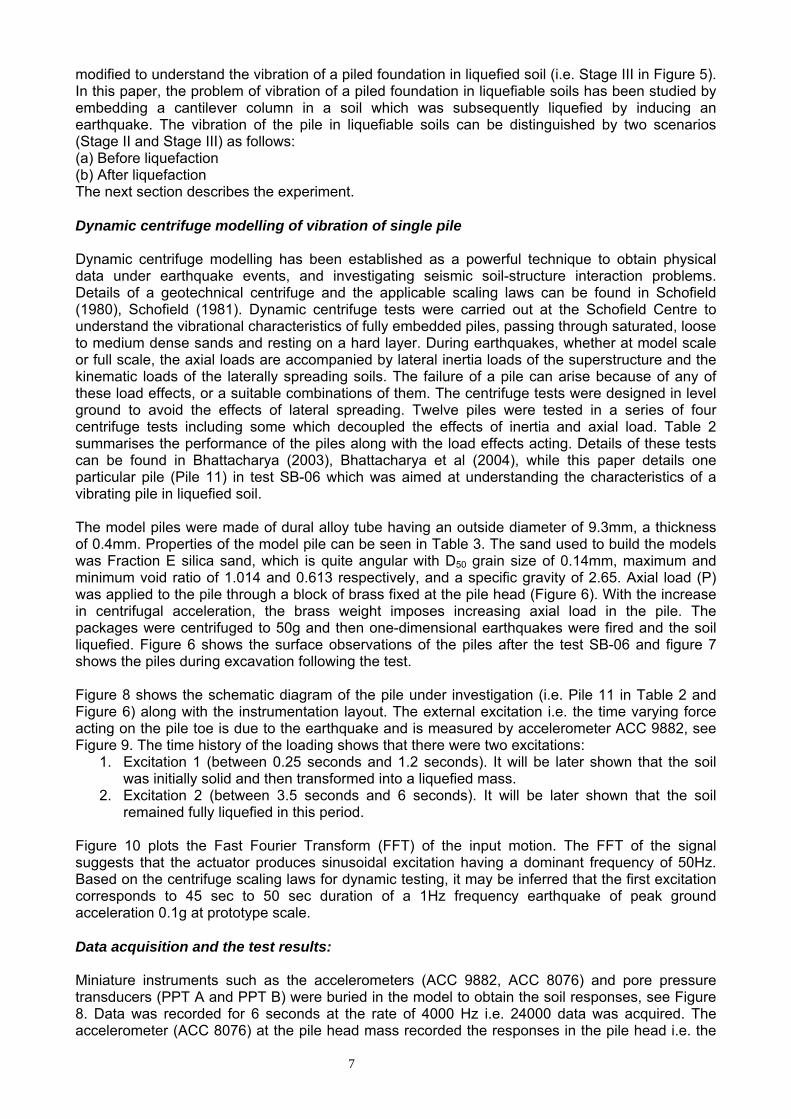
modified to understand the vibration of a piled foundation in liquefied soil (i.e. Stage III in Figure 5). In this paper, the problem of vibration of a piled foundation in liquefiable soils has been studied by embedding a cantilever column in a soil which was subsequently liquefied by inducing an earthquake. The vibration of the pile in liquefiable soils can be distinguished by two scenarios (Stage II and Stage III) as follows: (a) Before liquefaction (b) After liquefaction The next section describes the experiment. Dynamic centrifuge modelling of vibration of single pile Dynamic centrifuge modelling has been established as a powerful technique to obtain physical data under earthquake events, and investigating seismic soil-structure interaction problems. Details of a geotechnical centrifuge and the applicable scaling laws can be found in Schofield (1980), Schofield (1981). Dynamic centrifuge tests were carried out at the Schofield Centre to understand the vibrational characteristics of fully embedded piles, passing through saturated, loose to medium dense sands and resting on a hard layer. During earthquakes, whether at model scale or full scale, the axial loads are accompanied by lateral inertia loads of the superstructure and the kinematic loads of the laterally spreading soils. The failure of a pile can arise because of any of these load effects, or a suitable combinations of them. The centrifuge tests were designed in level ground to avoid the effects of lateral spreading. Twelve piles were tested in a series of four centrifuge tests including some which decoupled the effects of inertia and axial load. Table 2 summarises the performance of the piles along with the load effects acting. Details of these tests can be found in Bhattacharya (2003), Bhattacharya et al (2004), while this paper details one particular pile (Pile 11) in test SB-06 which was aimed at understanding the characteristics of a vibrating pile in liquefied soil. The model piles were made of dural alloy tube having an outside diameter of 9.3mm, a thickness of 0.4mm. Properties of the model pile can be seen in Table 3. The sand used to build the models was Fraction E silica sand, which is quite angular with D50 grain size of 0.14mm, maximum and minimum void ratio of 1.014 and 0.613 respectively, and a specific gravity of 2.65. Axial load (P) was applied to the pile through a block of brass fixed at the pile head (Figure 6). With the increase in centrifugal acceleration, the brass weight imposes increasing axial load in the pile. The packages were centrifuged to 50g and then one-dimensional earthquakes were fired and the soil liquefied. Figure 6 shows the surface observations of the piles after the test SB-06 and figure 7 shows the piles during excavation following the test. Figure 8 shows the schematic diagram of the pile under investigation (i.e. Pile 11 in Table 2 and Figure 6) along with the instrumentation layout. The external excitation i.e. the time varying force acting on the pile toe is due to the earthquake and is measured by accelerometer ACC 9882, see Figure 9. The time history of the loading shows that there were two excitations:

1. Excitation 1 (between 0.25 seconds and 1.2 seconds). It will be later shown that the soil was initially solid and then transformed into a liquefied mass.

2. Excitation 2 (between 3.5 seconds and 6 seconds). It will be later shown that the soil remained fully liquefied in this period.

Figure 10 plots the Fast Fourier Transform (FFT) of the input motion. The FFT of the signal suggests that the actuator produces sinusoidal excitation having a dominant frequency of 50Hz. Based on the centrifuge scaling laws for dynamic testing, it may be inferred that the first excitation corresponds to 45 sec to 50 sec duration of a 1Hz frequency earthquake of peak ground acceleration 0.1g at prototype scale. Data acquisition and the test results: Miniature instruments such as the accelerometers (ACC 9882, ACC 8076) and pore pressure transducers (PPT A and PPT B) were buried in the model to obtain the soil responses, see Figure 8. Data was recorded for 6 seconds at the rate of 4000 Hz i.e. 24000 data was acquired. The accelerometer (ACC 8076) at the pile head mass recorded the responses in the pile head i.e. the

8

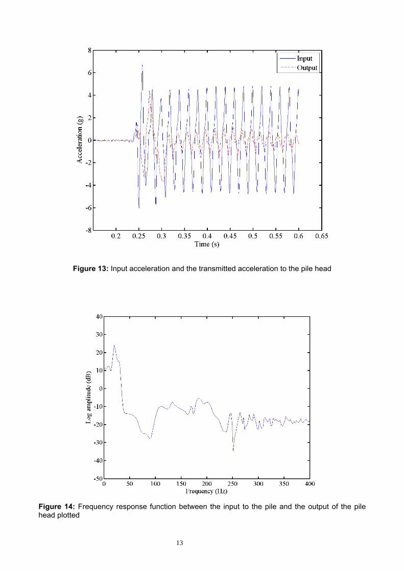
transfer of input acceleration to the pile head as soil transforms from a solid to a fluid-like medium. This change in response is due to the stiffness degradation of the pile-soil system. The pile head mass was not in contact with the liquefied ground and therefore the response is due to combined stiffness of the pile and the surrounding soil. Clearly, this is function of the stiffness and damping of the pile-soil system. Figures 11 and 12 show the traces of the excess pore pressure generated in the soil during the earthquake which provides us information regarding the onset of liquefaction. Figure 11 shows the traces of excess pore pressure during the entire 6 seconds of data acquisition while Figure 12 zooms in the initial time of shaking. The cyclic component of the PPT data behaviour is clearly due to shaking. It may be noted that as the shaking starts the excess pore pressure rises in the soil and reached a plateau almost instantly (at about 0.3 seconds). Figures 11 and 12 suggest that in each case, the plateau corresponds well with an estimate of the pre-existing effective vertical stress at the corresponding elevation, suggesting that the vertical effective stress had fallen to near zero value. In other words, the soil had liquefied. Just after about 0.3 sec, the pile would have lost all lateral effective stress from the soil i.e. the bracing action of the soil against buckling instability is almost negligible. Figure 13 plots the input acceleration (Input or the time history of accelerometer ACC 9882 in Figure 8) and the acceleration transmitted to the pile head (Output or time history of accelerometer ACC 8076 in Figure 8). It is interesting to note the change in the amplitude of vibration at the pile head during this period. The present paper is intended to improve understanding of this aspect of the vibration problem.

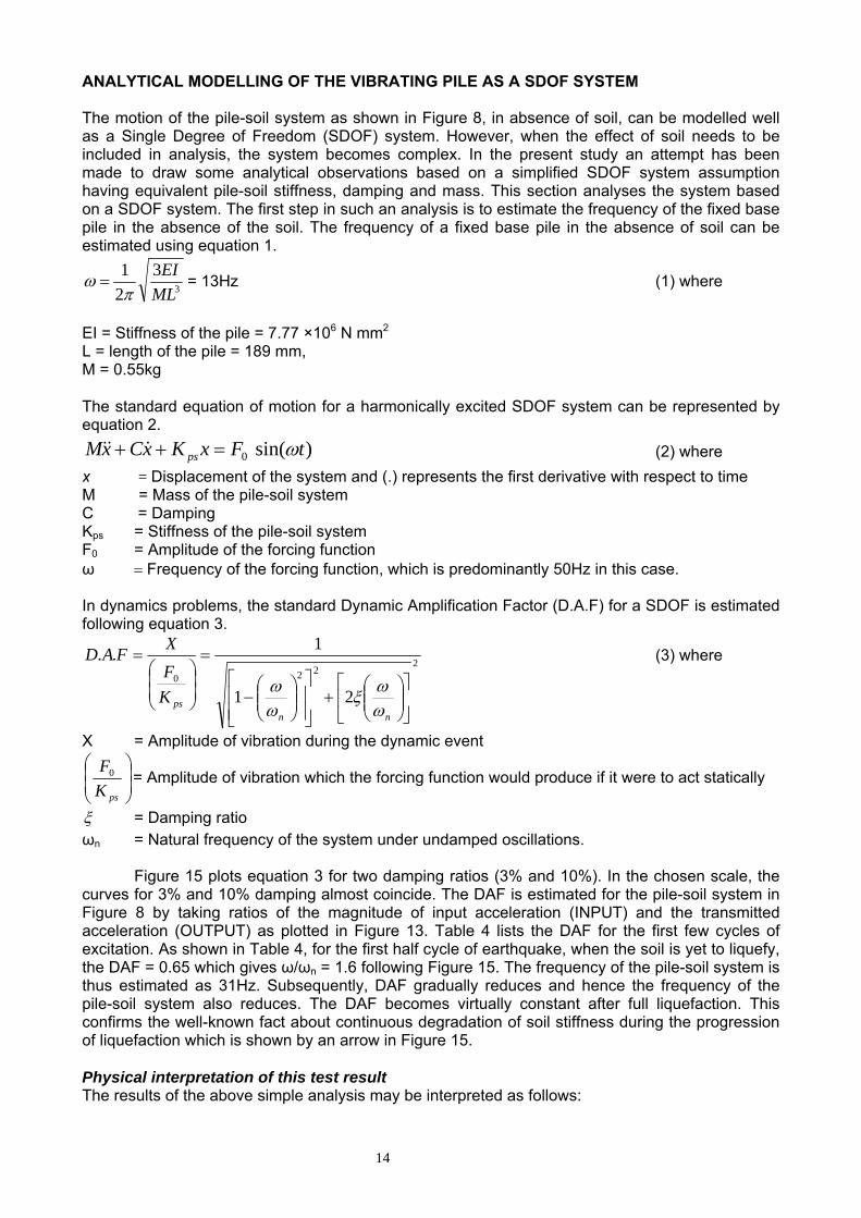
From this acceleration record, see Figure 13, it can be observed that the motion of the pile is initially in phase, i.e. at the onset of seismic shaking and in the first half cycle before soil started to liquefy. This is similar to Stage II in Figure 3. With the progression of liquefaction i.e. with the reduction of the stiffness of the pile-soil system, the motion of the pile is out of phase. After full liquefaction i.e., just after the instant of 0.3 sec in the time record, the motion of the pile comes in phase with the input acceleration. Figure 14 shows the frequency response function of the pile-soil system. This is essentially the ratio of the output and input of the pile plotted in the frequency domain. It may be seen that there is a peak at around 20Hz. As the input motion is predominantly harmonic and if we assume linear (between force and displacement) Single Degree of Freedom System (SDOF), then this peak would correspond to the natural frequency of the oscillator. The next section aims to investigate this aspect in more detail.

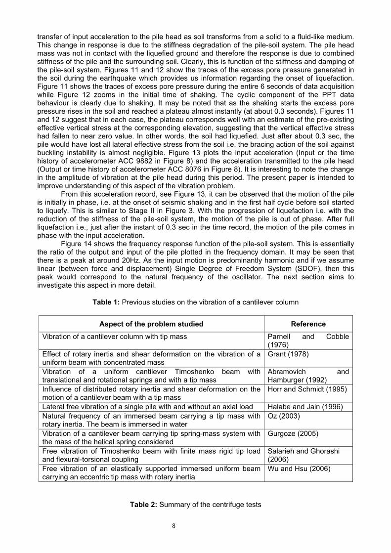
Table 1: Previous studies on the vibration of a cantilever column

Aspect of the problem studied Reference Vibration of a cantilever column with tip mass Parnell and Cobble

(1976) Effect of rotary inertia and shear deformation on the vibration of a uniform beam with concentrated mass

Grant (1978)

Vibration of a uniform cantilever Timoshenko beam with translational and rotational springs and with a tip mass

Abramovich and Hamburger (1992)

Influence of distributed rotary inertia and shear deformation on the motion of a cantilever beam with a tip mass

Horr and Schmidt (1995)

Lateral free vibration of a single pile with and without an axial load Halabe and Jain (1996) Natural frequency of an immersed beam carrying a tip mass with rotary inertia. The beam is immersed in water

Oz (2003)

Vibration of a cantilever beam carrying tip spring-mass system with the mass of the helical spring considered

Gurgoze (2005)

Free vibration of Timoshenko beam with finite mass rigid tip load and flexural-torsional coupling

Salarieh and Ghorashi (2006)

Free vibration of an elastically supported immersed uniform beam carrying an eccentric tip mass with rotary inertia

Wu and Hsu (2006)

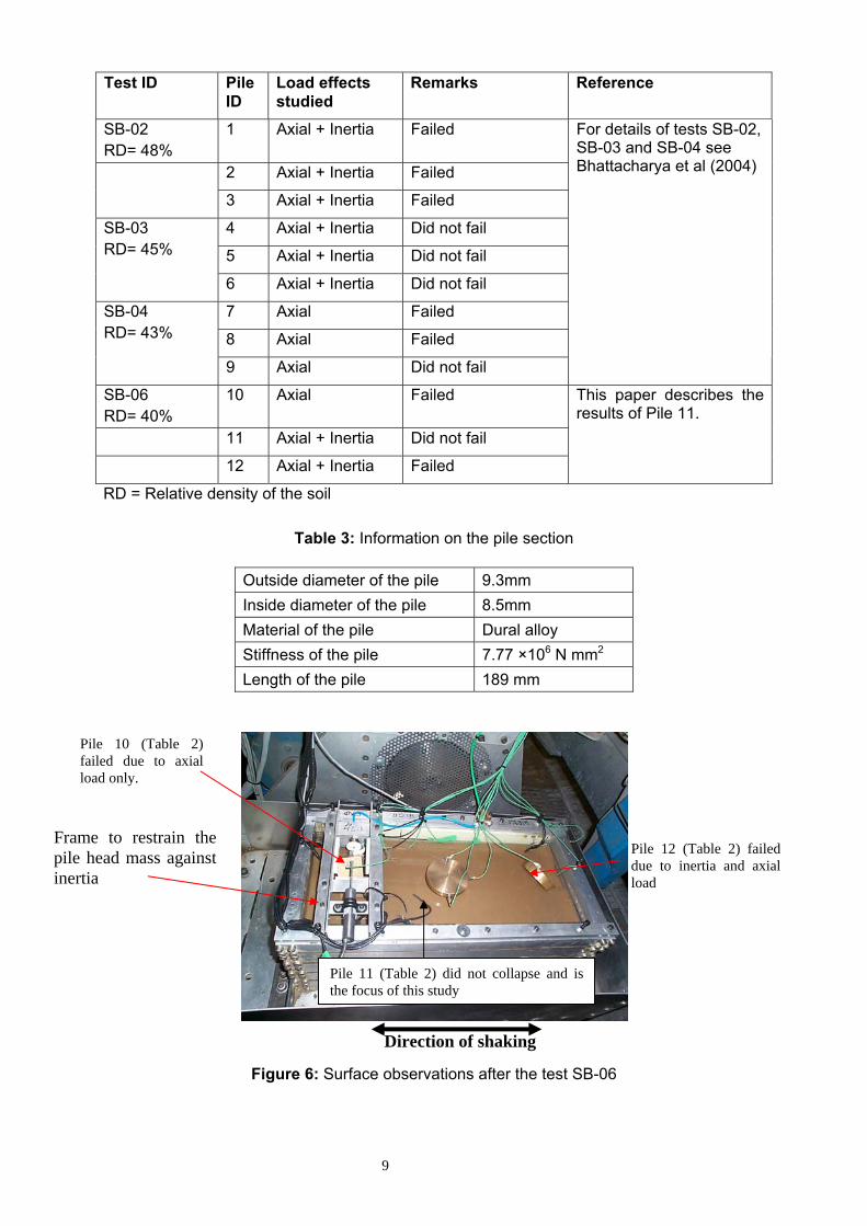
Table 2: Summary of the centrifuge tests

Test ID Pile ID

Load effects studied

Remarks Reference

SB-02 RD= 48%

1 Axial + Inertia Failed

2 Axial + Inertia Failed

3 Axial + Inertia Failed

4 Axial + Inertia Did not fail

5 Axial + Inertia Did not fail

SB-03 RD= 45%

6 Axial + Inertia Did not fail

7 Axial Failed

8 Axial Failed

SB-04 RD= 43%

9 Axial Did not fail

For details of tests SB-02, SB-03 and SB-04 see Bhattacharya et al (2004)

SB-06 RD= 40%

10 Axial Failed

11 Axial + Inertia Did not fail

12 Axial + Inertia Failed

This paper describes the results of Pile 11.

RD = Relative density of the soil

Table 3: Information on the pile section

Outside diameter of the pile 9.3mm Inside diameter of the pile 8.5mm Material of the pile Dural alloy Stiffness of the pile 7.77 ×106 N mm2

Length of the pile 189 mm

Pile 10 (Table 2) failed due to axial load only.

Frame to restrain the pile head mass against inertia

Pile 12 (Table 2) failed due to inertia and axial load

Figure 6:

Pile 11 (Table 2) did not collapse and is the focus of this study

9

Direction of shaking

Surface observations after the test SB-06

10

Figure 7: Piles 11 and 12 revealed during excavation in test SB-06

Figure 8: Schematic of Pile 11 and the instrumentation

11

Figure 9: Time history of the input acceleration (ACC 9882). The unit of acceleration is g.

Figure 10: FFT of the input signal shown in Figure 9

12

Figure 11: Pore pressure measurements

Figure 12: Time history of the pore pressure in the initial phase of the shaking

13

Figure 13: Input acceleration and the transmitted acceleration to the pile head

Figure 14: Frequency response function between the input to the pile and the output of the pile head plotted

14

ANALYTICAL MODELLING OF THE VIBRATING PILE AS A SDOF SYSTEM The motion of the pile-soil system as shown in Figure 8, in absence of soil, can be modelled well as a Single Degree of Freedom (SDOF) system. However, when the effect of soil needs to be included in analysis, the system becomes complex. In the present study an attempt has been made to draw some analytical observations based on a simplified SDOF system assumption having equivalent pile-soil stiffness, damping and mass. This section analyses the system based on a SDOF system. The first step in such an analysis is to estimate the frequency of the fixed base pile in the absence of the soil. The frequency of a fixed base pile in the absence of soil can be estimated using equation 1.

3

321

MLEI

πω = = 13Hz (1) where

EI = Stiffness of the pile = 7.77 ×106 N mm2

L = length of the pile = 189 mm, M = 0.55kg The standard equation of motion for a harmonically excited SDOF system can be represented by equation 2.

)sin(0 tFxKxCxM ps ω=++ &&& (2) where x = Displacement of the system and (.) represents the first derivative with respect to time M = Mass of the pile-soil system C = Damping Kps = Stiffness of the pile-soil system F0 = Amplitude of the forcing function ω = Frequency of the forcing function, which is predominantly 50Hz in this case. In dynamics problems, the standard Dynamic Amplification Factor (D.A.F) for a SDOF is estimated following equation 3.

2220

21

1..

⎥⎦

⎤⎢⎣

⎡⎟⎟⎠

⎞⎜⎜⎝

⎛+

⎥⎥⎦

⎤

⎢⎢⎣

⎡⎟⎟⎠

⎞⎜⎜⎝

⎛−

=

⎟⎟⎠

⎞⎜⎜⎝

⎛=

nnpsK

FXFAD

ωωξ

ωω

(3) where

X = Amplitude of vibration during the dynamic event

⎟⎟⎠

⎞⎜⎜⎝

⎛

psKF0 = Amplitude of vibration which the forcing function would produce if it were to act statically

ξ = Damping ratio ωn = Natural frequency of the system under undamped oscillations.

Figure 15 plots equation 3 for two damping ratios (3% and 10%). In the chosen scale, the

curves for 3% and 10% damping almost coincide. The DAF is estimated for the pile-soil system in Figure 8 by taking ratios of the magnitude of input acceleration (INPUT) and the transmitted acceleration (OUTPUT) as plotted in Figure 13. Table 4 lists the DAF for the first few cycles of excitation. As shown in Table 4, for the first half cycle of earthquake, when the soil is yet to liquefy, the DAF = 0.65 which gives ω/ωn = 1.6 following Figure 15. The frequency of the pile-soil system is thus estimated as 31Hz. Subsequently, DAF gradually reduces and hence the frequency of the pile-soil system also reduces. The DAF becomes virtually constant after full liquefaction. This confirms the well-known fact about continuous degradation of soil stiffness during the progression of liquefaction which is shown by an arrow in Figure 15. Physical interpretation of this test result The results of the above simple analysis may be interpreted as follows:

15

1. Initially before liquefaction and during the shaking, the pile-soil system acted as a coupled system. This can be justified by the fact that DAF is 0.65, which is very high when compared to the DAF expected if pile would have acted alone, which is approximately 0.1.

2. Once the surrounding soil liquefied, the frequency of the pile-soil system (18Hz) comes close to the frequency of the pile in absence of the soil i.e. about 13Hz.

The above observation hints to the fact that the stiffness of the liquefied soil should be ignored for all practical purposes while evaluating the response of piled foundations at full liquefaction.

Table 4: Observed Dynamic Amplification Factor (D.A.F)

Cycle of earthquake D.A.F

(from Figure 6) ω/ωn

(from graph 7) Frequency of pile-soil

system 1st Half-cycle 0.65 1.6 31Hz 2nd Half-cycle 0.43 1.75 29Hz 8th Half-cycle and onwards

0.17 2.8 18Hz

ω = forcing frequency = 50Hz [See Figure 10]

Figure 15: Dynamic amplification factor for a SDOF system.

ESTIMATION OF OPTIMAL PARAMETERS OF AN EQUIVALENT SDOF SYSTEM This section aims to obtain the dynamic parameters of an equivalent SDOF oscillator (i.e. the natural frequency and the damping factor) from the measured frequency response function shown in Figure 14. In a vibration problem, the damping of the system controls the maximum amplitude of vibration (see equation 3). In the present problem this would affect the bending moment of the pile along the depth. In order to estimate the maximum amplitude of vibration in a SDOF system (following equation 3), we have two unknowns: the damping factor (ξ ) and the natural frequency ( nω ). Table 5 lists the uncertainty in the estimation of the parameters for the problem under consideration. In this section, a non-linear least square approach has been used to obtain dynamic parameters of an equivalent SDOF system corresponding to the measured frequency response. The normalised dynamic response of a SDOF system can be obtained as

16

⎟⎟⎠

⎞⎜⎜⎝

⎛+⎟⎟

⎠

⎞⎜⎜⎝

⎛−

==

=

nn

ix

xd

ωωζ

ωωω

ωω

21

1)0(

)()( 2 (4)

The dynamic amplification factor is defined as

222

21

1)()()(

⎟⎟⎠

⎞⎜⎜⎝

⎛⎟⎟⎠

⎞⎜⎜⎝

⎛+

⎟⎟

⎠

⎞

⎜⎜

⎝

⎛⎟⎟⎠

⎞⎜⎜⎝

⎛−

== ∗

nn

ddd

ωως

ωω

ωωω (5)

where denotes the complex conjugation. If the experimentally measured dynamic response is denoted by

( )∗•)(ωg , the frequency dependent complex valued “error” is given as:

)()()( ωωωε dg −= (6)

It must be mentioned that the parameters nω and ξ are unknown in our fitted model. It is aimed to obtain these parameters such that the norm of the above error is minimised across the range of frequency considered. Let us assume this frequency range lies between [ ]Ω,0 . Using the standard l2 norm, the objective function can be expressed as:

∫∫Ω∈

∗

Ω∈

==ωω

ωωεωεωωεχ dd )()()(22 (7)

The two unknown parameters can be obtained using the following two equations.

02

=∂∂

nωχ

(8)

and

02

=∂

∂ς

χ (9)

In the experimental measurements )(ωg is obtained at discrete frequency points. Equations 8 and 9 were solved numerically using Matlab and is shown in Figure 16. Figure 16 shows the fitted SDOF model to the measured data. The optimisation shows that the equivalent natural frequency of the SDOF system is about 19.42 Hz and the damping provided by liquefied soil is about 11%. The equivalent natural frequency of the oscillator obtained from non-linear least square error minimisation method agrees quite well with the simple graphical method listed in Table 3. It must be mentioned that the obtained damping co-efficient of the oscillator is independent of stiffness and can therefore can be used for design purposes. Table 5: Uncertainty in the parameters for identification of the damping provided by liquefied soil to

the vibrating pile Term in Equation 2 Certain/ uncertain Remarks Mass The pile head mass is certain

and fully known. In SDOF model assumption, the mass of the beam is neglected and therefore the mass of the vibrating liquefied soil can also be neglected.

Stiffness The stiffness of the pile is fully known, but there are uncertainties in the soil stiffness which also makes the combined stiffness (kps) uncertain.

It is however known that the stiffness of the soil reduces drastically with the onset of liquefaction

Damping This is completely unknown

One of the main aims of this study is to identify the damping characteristics of liquefied soil.

Forcing function Fully known and certain This is measured using the accelerometer ACC 9882

17

Figure 16: Fitted equivalent SDOF system

PRACTICAL IMPLICATIONS AND DISCUSSION Theory of forced vibrations would dictate that the performance of fully-embedded end-bearing “structurally stable” piled foundation under fully-liquefied condition will depend on its first natural frequency at full liquefaction and the fundamental driving frequency of the earthquake. In practice, three conditions may arise (see Figure 15) depending on the magnitude of ω (fundamental driving frequency of the earthquake) and ω1 (first natural frequency of the piled foundation under fully liquefied condition):

• 5.01

≤ωω

. In such cases, the lateral deflection of the piled building would increase by a

maximum of 33% than the amount by which the building would have deflected if the earthquake force would have acted statically.

• 5.15.01

≤<ωω

. This is the dangerous range and should be avoided. If the ratio is in the

vicinity of 1, resonance would occur leading to dynamic failure.

• 5.11

>ωω

. This is the safe zone and the deflections are not amplified. Higher the ratio lesser

is the amplitude of vibration.

In spite of the valuable insights regarding the effects of reduction of the first natural frequency of a foundation, modelling the vibration of a pile in liquefied soil as SDOF system has many limitations. For example, the rotary inertia of the building or the pile head mass is not taken into consideration. Most crucially, perhaps, the effect of the axial load coming from the superstructure has been ignored. As a result, the dynamic instability effects arising due to the axial force has also been

18

ignored. The companion paper carries out a rigorous modeling of this problem and also highlights the importance of this consideration in design by analyzing the failure of the building described in Figure 1. CONCLUSIONS Characteristics of the vibration of a piled foundation in liquefiable soils are studied using a geotechnical centrifuge. In the experiment, a small-scale vibrating cantilever pile with a tip mass is immersed in a liquefied soil and the structural responses are recorded. A Single Degree of Freedom (SDOF) model has been fitted to the experimental data. This study suggests the following:

1. Before partial or full liquefaction and during the initial period of shaking, the soil surrounding the pile provides stiffness and damping to the vibrating piled structure. After liquefaction, the stiffness of the soil reduces to near zero value and the liquefied soil predominantly provides damping to the motion of the piled structure. The stiffness of the liquefied soil should therefore be ignored for all practical purposes for evaluating the response of the piled foundations at full liquefaction.

2. The first natural frequency of a piled foundation (i.e. frequency for free vibration) reduces with the increase in pore pressure in the surrounding soil i.e. with the progression of liquefaction. The reduction of this frequency will be lowest when the soil surrounding the pile is in fully liquefied state. Results of a dynamic centrifuge tests suggest that liquefied soil offers a damping of about 11% to a vibrating pile.

19

REFERENCES: 1. Abdoun, T. H and Dobry, R (2002): “Evaluation of pile foundation response to lateral

spreading”, Soil Dynamics and Earthquake Engineering, No 22, pp 1051-1058. 2. Abramovich, H., and Hamburger, O., 1992, ‘‘Vibration of a Cantilever Timoshenko Beam

with Translational and Rotational Springs and with Tip Mass,’’ Journal of Sound and Vibration, 154, pp. 67–80.

3. B.T.L (2000) BTL Committee (2000): Study on liquefaction and lateral spreading in the 1995 Hyogoken-Nambu earthquake, Building Research Report No 138, Building Research Institute, Ministry of Construction, Japan (in Japanese).

4. Bhattacharya, S (2003): “Pile instability during earthquake liquefaction”, PhD thesis, Cambridge University (U.K).

5. Bhattacharya, S. Madabhushi, S.P.G and Bolton, M.D (2004): “An alternative mechanism of pile failure in liquefiable deposits during earthquakes”, Geotechnique 54, Issue 3 (April), pp 203-213.

6. Bhattacharya, S., Madabhushi, S.P.G. and Bolton, M.D (2005a): Authors reply to the discussion on “An alternative mechanism of pile failure in liquefiable deposits during earthquakes”, Geotechnique 55, Issue 3 (April), pp 259-263.

7. Bhattacharya, S., Madabhushi, S.P.G. and Bolton, M.D (2005b): “A reconsideration of the safety of piled bridge foundations in liquefiable soils”, Soils and Foundations, Volume 45, No 4, pp 13-25, August 2005.

8. Bhattacharya, S and Bolton, M.D (2004): “A fundamental omission in seismic pile design leading to collapse” Proceedings of the 11th International Conference on soil dynamics and Earthquake Engineering, 7th to 9th Jan 2004, Berkeley, Volume 1, pp 820-827

9. Grant, D.A. (1978): “The effect of rotary inertia and shear deformation on the frequency and normal mode equations of uniform beams carrying a concentrated mass”, Journal of Sound and Vibration, 57(3), pp 357-365.

10. Gurgoze, M. (2005): “On the Eigen frequencies of a cantilever beam carrying a tip spring-mass system with mass of the helical spring considered”, Journal of Sound and Vibration, 282, pp 1221-1230.

11. Halabe, U.B. and Jain, S.K. (1996): “Lateral free vibration of a single pile with and without an axial load”, Journal of Sound and Vibration, 195(3), 531-544.

12. Hamada, M (1992): “Case Studies of liquefaction and lifelines performance during past earthquake”, Technical Report NCEER-92-0001, Volume-1, Japanese Case Studies, National Centre for Earthquake Engineering Research, Buffalo, NY.

13. Horr, A.M. and Schmidt, L.C. (1995): “Closed-form solution for the Timoshenko beam theory using a computer-based mathematical package”, Computers & Structures, Volume 55, No 3, pp 405-412

14. Ishihara, K (1997): Terzaghi oration: “Geotechnical aspects of the 1995 Kobe earthquake”, Proc of ICSMFE, Hamburg.

15. JRA (2002): Japanese Road Association, Specification for Highway Bridges, Part V, Seismic Design

16. Knappett and Madabhushi, S.P.G. (2005): “Modelling of Liquefaction-induced instability in pile groups”. ASCE Special Publication No 145 on “Seismic Performance and Simulation of Pile Foundations in Liquefied and Laterally Spreading Ground”.

17. Oz, H.R (2003): “Natural frequency of an immersed beam carrying a tip mass with rotatory inertia”, Journal of Sound and Vibration, 266, pp 1099-1108.

18. Salarieh, H and Ghorashi, M (2006): “Free vibration of Timoshenko beam with finite mass rigid tip load and flexural-torsional coupling”, International Journal of Mechanical Sciences, pp 763-779.

19. Schofield, A. N. (1981): “Dynamic and Earthquake Geotechnical Centrifuge Modelling”, Proceedings of the International Conference Recent Advances in Geotechnical Earthquake Engineering and Soil Dynamics, Vol. 3, 1081-1100.

20. Schofield, A. N. (1980): “Cambridge Centrifuge operations”, Twentieth Rankine Lecture. Geotechnique, London, England, Vol. 30, 227-268.

21. Parnell, L. A., and Cobble, M. H., 1976, ‘‘Lateral Displacements of a Vibrating Cantilever Beam with a Concentrated Mass,’’ J. Sound Vib., 44, pp. 499–511.

20

22. Tokimatsu K. and Asaka Y (1998): “Effects of liquefaction-induced ground displacements on pile performance in the 1995 Hyogeken-Nambu earthquake”, Special issue of Soils and Foundations, pp 163-177, Sep 1998.

23. Wu, J-S and Hsu, S-H (2006): “A unified approach for the free vibration analysis of an elastically supported immersed uniform beam carrying an eccentric tip mass with rotary inertia”, Journal of Sound and Vibration, 291, pp 1122-1147.

24. Yoshida, N and Hamada, M. (1990): Damage to foundation piles and deformation pattern of ground due to liquefaction-induced permanent ground deformation, Proceedings of 3rd Japan-US workshop on Earthquake Resistant design of lifeline facilities and countermeasures for soil liquefaction, pp 147-161.

21

Vibrational characteristics of a piled structure in liquefied soil during earthquakes: Part II (Analytical modelling)

Subhamoy Bhattacharya and Sondipon Adhikari

ABSTRACT This paper addresses the vibrational characteristics of piles in liquefiable soils under earthquake loading. Part 1 of this companion paper studied this vibration problem using high quality experimental data obtained from dynamic centrifuge tests. This paper presents a rigorous analytical solution of the same problem based on Euler-Bernoulli beam theory. The pile has been modelled as a beam on elastic foundation carrying a tip mass and having rotary inertia. The natural frequency of the pile is obtained in terms of useful non-dimensional parameters. The practical implication of this research has been highlighted by considering the behaviour of a well-documented case history of a pile-supported building during the 1995 Kobe earthquake (Japan). Keywords: Pile, failure, resonance, Instability, Damping INTRODUCTION Collapse and/or severe damage of pile-supported structures is still observed in liquefiable soils after most major earthquakes such as the 1995 Kobe earthquake (JAPAN), the 1999 Kocheli earthquake (TURKEY), and the 2001 Bhuj earthquake (INDIA). The failures not only occurred in laterally spreading (sloping) ground but were also observed in level ground where no lateral spreading would be anticipated; see for example Tokimatsu and Asaka (1998). The failures were often accompanied by settlement and tilting of the superstructure, rendering it either useless or very expensive to rehabilitate after the earthquake. Following the 1995 Kobe earthquake, investigations has been carried out to find the failure pattern of the piles; see Yoshida and Hamada (1990), BTL (2000). Piles were excavated or extracted from the subsoil, borehole cameras were used to take photographs, and pile integrity tests were carried out. These studies hinted the location of the cracks and damage patterns for the piles. Of particular interest is the formation of plastic hinges in the piles. This indicates that the stresses in the pile during and after liquefaction exceeded the yield stress of the material of the pile, despite large factors of safety were employed in the design. As a result, design of pile foundation in seismically liquefiable areas still remains a continuing area of concern for the earthquake geotechnical engineering community. “Slender piles passing through water or thick deposits of very weak soil need to be checked against buckling. This check is not normally necessary when piles are completely embedded in the ground unless the characteristic undrained shear strength is less than 15kPa”. Bhattacharya (2003), Bhattacharya et al (2004, 2005), Knappett and Madabhushi (2005) have shown that where saturated sands liquefy in earthquakes, the soil bracing effect would be eliminated and slender foundation piles would buckle. This has led to an obvious design criteria that piled foundation should vibrate back and forth in liquefiable soils during earthquakes and must return to its original configuration at the end of the earthquake. In other words, the vibration of the pile would shear the liquefied soil. The amplitude of the displacement of vibration of the piles should be such that the pile should never become unstable under the P-delta effect i.e. should never reach the point from which there is no return. In addition, the stress in any section of the pile should not reach the yield stress i.e. obeying the lower bound theorem of plasticity.

22

Part 1 of this paper investigated this problem using high quality experimental data obtained from dynamic centrifuge tests. In the experiment, a cantilever pile with a tip mass was embedded in a saturated sandy deposit and the soil was subsequently liquefied through an earthquake. The tip mass represented the vertical building loads which tend to buckle the piles. This particular configuration was chosen as this represents the simplest form of vibrating system. The response of the pile head mass was measured as the soil transformed from being solid to liquid. The experimental data has been analysed based on SDOF system and the following conclusions have been drawn:

1. Before the liquefaction and during the initial shaking, the soil surrounding the pile provides stiffness and damping to the vibrating pile.

2. After liquefaction, the stiffness of the soil reduces to near zero value and the liquefied soil provides predominantly damping to the motion of the pile. The measured damping factor in the first mode is about 11%.

3. The stiffness of the liquefied soil should be ignored for all practical purposes to evaluate the response of the piled foundations at full liquefaction.

In spite of these insights, modelling the problem of vibration of pile in liquefied soil as a SDOF system poses the following limitations:

(a) In a SDOF system analysis, it is assumed that the mass of the beam is negligible compared to the tip mass. However, in reality the mass of the piles can be more than 10% of the mass of the building. This will be shown later on through an example.

(b) The linear and rotary inertia of the mass of building (tip mass in the model test reported in the companion paper) is not considered in the analysis. However, it has been observed in centrifuge tests that the pile head mass rotates. Study of field case records also suggests that the superstructure of the collapsed pile-supported structures also rotated. This suggests that linear and rotary inertia should be taken into consideration while analysing the vibration of a piled building.

(c) The distributed nature of the support of the surrounding soil to the pile has not been taken into account. The nature of this support will vary in the duration of the earthquake. The support will substantially reduce following the liquefaction.

(d) Most crucially, perhaps, the affect of the axial load on the pile coming from the superstructure has been ignored. As a result, the dynamic instability effects arising due to the axial force has also been ignored.

This paper analyses the problem of a vibrating pile in liquefied soil using Euler-Bernoulli beam theory. The pile has been modelled as a beam with distributed inertia and stiffness properties. The proposed analysis is aimed at addressing the dynamic instability of piles in a rigorous manner. Most importantly, the study also aims to verify if the existing simplified approach such as JRA (2002), AIJ (2001) where the dynamic effects has been ignored can be considered conservative. The authors however recognise that codes of practice have to specify some simplified approach for design which should provide a safe working envelope for any structure of the class being considered, and in full range of ground conditions likely to be encountered at different sites. Our concern in this paper is not to criticise provisions of the existing codes of practice but to point out that the application of such simplified approach demands further consideration of effective lateral stiffness of the pile taking into the account the change in natural frequency of the structure during liquefaction i.e. in the transient phase. In this study, the main focus is on the first natural frequency of the pile in the transition phase when the soil transforms from being solid to liquid. Intuitively, it appears that as the soil liquefies, the first natural frequency of the building will drop. If the first natural frequency of the pile comes close to the excitation frequency of the earthquake motion (typically between 0.5 Hz and 10Hz), then the amplitude of vibration will grows exponentially even in the presence of damping – the phenomenon being resonance. For a pile, the deflection will increase and so the stresses. The question whether such situation may arise to cause resonance in a piled foundation that may promote dynamic instability in the manner set out above will be explored in this paper.

23

Dynamic instability of elastic structures has received extensive attention during the past four decades due to failure of many engineering structures, in which large deformations were observed. The books by Thompson and Hunt (1973), Timoshenko Young and Weaver (1974), Leipholz (1975) are referred for further reading. COMPARISON OF THE PROPOSED WORK WITH CURRENT RECOMMENDED PRACTICE It is considered useful to review the analytical approach behind the standard practice for seismic pile design in liquefiable soils. In this regard the AIJ (2001) is chosen. The Architectural Institute of Japan (AIJ) in the 2001 edition of the code titled “Recommendations for design of building foundations” recommends the following. The equation of the pile is expressed by Euler-Bernoulli beam equation with a distributed elastic support as

( )gph yyBkdz

ydEI −−= .4

4

(1) where z = Depth y(z) = Pile displacement in the transverse direction yg = Ground displacement EI = Flexural rigidity of the pile The coefficient of the subgrade reaction kh is given by equation (2) as follows:

1

1

1

2

yy

kkr

hh

+=

β

(2) where

75.0001 ..80 −= BEkh

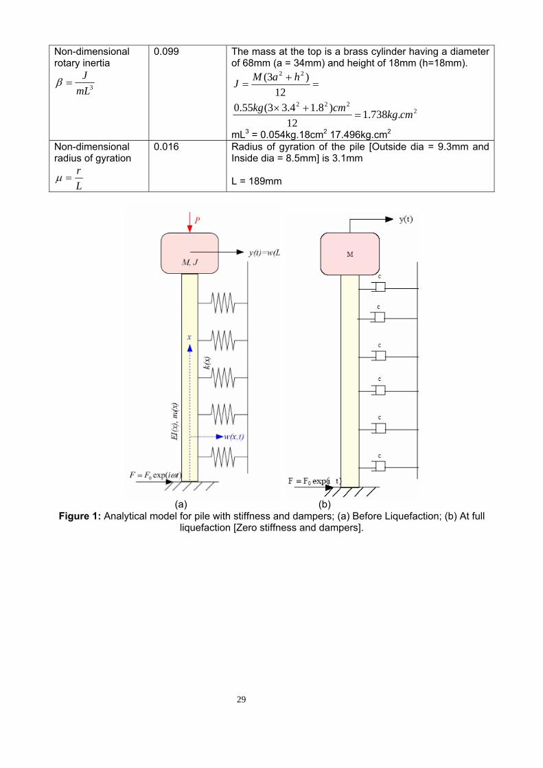
E0 = 0.7N in the units of MN/m2 and N is the SPT value β = Scaling factor for liquefied soil. The value is generally 1 for non-liquefied sand and 0.1 for liquefied sand. B0 = Pile diameter in cm yr = Relative displacement between pile and the soil = (y-yg) y1 = Reference value of yr. This is often used as 1% of pile diameter. Clearly equation (1) is based on static considerations and it does not take account of any dynamic effects which can be crucial during an earthquake. More critically, the effects of static axial load are also ignored. The next section of the paper formulates the dynamic equations of motion taking into account the axial load. ANALYTICAL INVESTIGATION Modelling the vibrating pile as a beam with distributed mass resting on springs k(x) and dampers (c)and supporting a tip mass (M) having a rotary inertia (J) Based on the experimental evidence described in the first part of the paper, Figure 1(a) idealises the pile before liquefaction. At this stage, the soil has adequate stiffness and can be replaced by spring stiffness and dampers. On the other hand, Figure 1(b) idealises the pile at full liquefaction where the soil surrounding the pile is under fully liquefied condition. In this case, the soil is replaced by dampers as the stiffness is near zero value. It must be mentioned that the stiffness of liquefied soil is mobilised after considerable amount of strain as has been reported by various researchers such as Takahashi et al (2002), Towhata et al (1999).

24

The main assumptions in our proposed analysis are: (1) The inertial and the elastic properties of the pile are constant along the depth of the pile. (2) The soil stiffness is elastic and linear, continuous and varies along the depth shown by k(x).

The variation of k(x) with lateral displacement (y) which is often known as “p-y” curves is not considered in the present analysis. This assumption is being used bearing in mind that soil behaves elastically at very small strains. As this investigation deals with the transition from full soil stiffness to zero soil stiffness (liquefied), this assumption will not mask the behaviour under investigation.

(3) The boundary condition at the bottom of the pile can be considered as fixed (that is no rotation and no displacement is allowed). This would represent a pile embedded in the non-liquefiable dense layer where strain-induced degradation is relatively negligible.

(4) The tip mass is rigidly attached to the pile head. (5) The axial force in the pile is constant and remains axial during vibration. (6) Deflections due shear force are negligible and a plain section in the pile remains plane

during the bending vibration (standard assumptions in the Euler-Bernoulli beam theory). (7) None of the properties are changing with time. In other words, the system is time invariant.

Governing equations Let us assume that the bending stiffness of the beam may vary along the length and is therefore denoted by EI(x). The beam is resting against a linear uniform elastic support of stiffness k(x). The beam has a tip mass (M) with rotary inertia J. The mass per unit length of the beam is m and r is the radius of gyration. The beam is subjected to a constant compressive axial load P. Using the Hamilton’s principle, the equation of motion of the beam is given by the following fourth-order partial differential equation:

( ) ( ) ),(),(.),().(),()(.,),()( 22

2

2

2

txftxwmtxwxkx

txwxrmxx

txwxPxx

txwxEIx

=++⎟⎠⎞

⎜⎝⎛

∂∂

∂∂

−⎟⎠⎞

⎜⎝⎛

∂∂

∂∂

+⎟⎟⎠

⎞⎜⎜⎝

⎛∂

∂∂∂

&&&&

(3), where ),( txw = Transverse deflection of the beam

t = Time ),( txw&& = Second derivative with respect to time i.e. acceleration

P(x) = Axial load )(2 xmr = Moment of inertia of the beam

),( txf = Time dependent load on the beam It is important to distinguish the difference between equations 1 and 3. Equation 1 is based on static consideration ignoring the effects of axial load and most importantly, the dynamic considerations.

It is difficult to find a closed form solution for equation 3 and is therefore considered appropriate to solve the equation using numerical techniques for different boundary conditions at the top and bottom of the pile. In this paper, we wish to demonstrate the change in the natural frequency of the piled foundation when the soil liquefies i.e. when the support stiffness k(x) reduces. It is important to remember that AIJ (2000) recommends that the stiffness of the soil reduces by 90% during full liquefaction (see equation 2).

Before equation 3 is solved in a generalised form, we consider a simple boundary conditions for which a closed-form solution exists. This would allow us to gain some physical understandings that may be extended to the generalised case. We therefore consider a pinned-pinned beam having uniform bending stiffness (EI) supported on uniform linear springs of stiffness (k) as shown in figure 2. The next section discusses this case. Pinned-Pinned beam supported on elastic springs carrying an axial load P

25

This section of the paper analyses the special case for pined-pinned beam having uniform stiffness carrying an axial load (P) and resting against on a uniform elastic support (k) as depicted in Figure 2. For the free vibration problem, = 0 and equation 3 reduces to equation 4. ),( txf

( ) 0),(.),(.),(.,),(2

22

2

2

4

4

=++∂

∂−⎟⎟

⎠

⎞⎜⎜⎝

⎛∂

∂+⎟⎟

⎠

⎞⎜⎜⎝

⎛∂

∂ txwmtxwkx

txwrmx

txwPx

txwEI &&&&

(4)

The four boundary condition associated with this problem can be expressed as follows: (1) Deflection is zero at x=0 and x=L, and therefore

0),0( =tw (4a) 0),( =tLw (4b)

(2) Bending moment is zero at x=0 and x=L and therefore 0),0( =′′ tw (4c) 0),( =′′ tLw (4d)

The non-dimensional natural frequency of the beam is given by equation 5. Details of the solution can be found in Appendix A.

⎟⎠⎞

⎜⎝⎛ +−

+=Ω 442222

442 /

1..1 π

ηπµ

πnn

PPn

n crn (5), where

Ωn = Effective non-dimensional nth natural frequency of the beam given by equation 6

EImL

n

422 ω=Ω (6)

n = Mode number, n = 1,2,3,….

η = Non-dimensional support stiffness given by EIkL4

=η (7)

µ = Non-dimensional radius of gyration Lr

=µ (8)

r = Radius of Gyration of the section of the beam L = Length of the beam P = Axial Load on the beam

Pcr = Euler’s Critical Load for pinned-pinned strut and is given by 2

2

LEIπ

From equation 5, two inferences can be drawn:

1. The natural frequency of the beam reduces with the increase in axial load (P) i.e. with the Euler’s load ratio (P/Pcr).

2. The natural frequency of the beam increases with the support stiffness (η). This is widely accepted by all seismic codes of practice, such as IS: 1893, NEHRP (2000). As a result, the time period of a building supported on piled foundations is calculated based on the configuration of the superstructure (height and width) ignoring the effects of the foundation. It is generally accepted that the soil provides adequate support.

Case 1: Zero support stiffness (η = 0). The physical interpretation is the soil surrounding the pile is in fully liquefied state. Under such condition, if the applied axial load P is equal to Euler’s Critical Load (Pcr), the frequency Ωn is zero. This also implies that buckling can be viewed as a point when the effective natural frequency of a system is zero. Case 2: Transient phase when the soil surrounding the pile is being transformed to a liquid (η decreasing with time).

26

For a fixed axial load P acting on the beam, as the soil stiffness decreases i.e. η decreases, equation 5 suggests that Ωn also decreases. This implies that during the process of liquefaction, the effective natural frequency of the pile will decrease. If the frequency comes close to the earthquake excitation frequency, resonance may be expected. In the next section, we investigate if a piled foundation can fail by resonance as the soil surrounding the pile liquefies in an earthquake. This investigation is based on the dynamic centrifuge tests reported in Part 1 of this paper and also by considering a well-documented case history. Vibration of a cantilever pile in the dynamic centrifuge test reported in the companion paper This section of the paper solves the vibration of the cantilever pile described in the companion paper and shown in Figure 1 (a&b). As we are interested in free vibration problem, = 0. ),( txf The four boundary conditions associated with this problem are:

(1) Deflection is zero at x=0 and therefore 0),0( =tw (9)

(2) Rotation is zero at x=0 and therefore 0),0( =′ tw (10)

(3) Bending moment is zero at x=L

0),(),(2

2

=∂

∂+⎟⎟

⎠

⎞⎜⎜⎝

⎛∂

∂x

tLwJx

tLwEI&&

(11)

(4) Shear Force is zero at x=L ( ) 0),(.),(,),( 2

3

3

=⎟⎠⎞

⎜⎝⎛

∂∂

−−⎟⎠⎞

⎜⎝⎛

∂∂

−⎟⎟⎠

⎞⎜⎜⎝

⎛∂

∂x

tLwrmtLwMx

tLwPx

tLwEI&&

&& (12)

The above problem must have a harmonic solution and using separation of variables, we assume that the solution is of the form given by equation 13.

tieWtxw ωξ ).(),( = (13), where

Lx

=ξ

Substituting equation 13 in the equation of motion (equation 3), results in equation 14.

0)(.)(..)(.)()(2

2

2

222

2

2

24

4

4 =∂

∂+−+

∂∂

+∂

∂ξ

ξωξωξξ

ξξ

ξ WLrmWmWkW

LPW

LEI (14)

It is convenient to express equation 14 in terms of non-dimensional parameters. Elementary rearrangement of equation 14 gives equation 15.

0)(.)(..)(.)()(2

2222424

2

22

4

4

=∂

∂+−+

∂∂

+∂

∂ξ

ξωξωξξ

ξξ

ξ WEI

LrmWEI

LmWEIkLW

EIPLW (15)

The following non-dimensional parameters are chosen: Non-dimensional Axial Force

⎟⎟⎠

⎞⎜⎜⎝

⎛==

crPP

EIPL

4

22 πν (16)

where

2

2

4LEIPcr

π= commonly known as “Critical Load” or “Euler’s Buckling Load” for a cantilever strut.

27

Non-dimensional support stiffness

EIkL4

=η (17)

Non-dimensional Frequency Parameter

EImL4

22 ϖ=Ω (18)

Non-dimensional mass ratio

mLM

=α (19)

Non-dimensional Rotary Inertia

3mLJ

=β (20)

Non-dimensional radius of gyration

Lr

=µ (21)

Equation 15 can be expressed in non-dimensional form as shown in Equation 22

0)(.)(.)()()( 22

222

4

4

=Ω−+∂

∂Ω++

∂∂ ξξη

ξξµν

ξξ WWWW (22)

Equation 22 can be rearranged as

0)().()()()( 22

222

4

4

=−Ω−∂

∂Ω++

∂∂ ξη

ξξµν

ξξ WWW (23)

The boundary conditions given by equations (9) – (12) can also be transformed in terms of the non-dimensional parameters introduced above and the associated eigenvalue problem can be solved to obtain the natural frequencies of the system. The details of the solution procedure are given in Appendix B. For most piles, non-dimensional radius of gyration 1<<µ , so that . Therefore, for low frequency vibrations,

02 ≈µνν =~ . The frequency equation of the system is given by either equation

(B.27) or equation (B.34) depending on two parametric cases discussed in Appendix B. These transcendental equations are solved numerically using Matlab in this paper. Once the non-dimensional frequency Ω is obtained by solving these equations, the actual natural frequency of the piles can be obtained from equation (18) as

4

EImL

ϖ = Ω

The next section numerically solves the vibration problem for the particular boundary condition for the model pile described in the companion paper. Table 1 lists the non-dimensional parameters defined by Equations 16 through 21 for the experimental test results reported in the companion paper. The most uncertain parameter in the experiment is the stiffness of the soil. The stiffness of the soil prior to liquefaction has been estimated based on the API (2000). It is well known that the stiffness of the soil drops drastically with the rise in pore pressure. Following the recommendations of the Japanese Code (AIJ 2000) the stiffness of the soil is reduced to 90% to consider the effects of liquefaction (see Equation 2). Results of the analysis This section plots and discusses the results for Pile 11 described in the companion paper. Figure 3 plots the variation of the first natural frequency of the beam (ω1) with the axial load ratio or the (P/Pcr) ratio for different support stiffness (η). The support stiffness was gradually reduced to about

28

8% of the original stiffness to simulate the condition of full liquefaction following AIJ (2001). This reduction has been shown by the arrow in Figure 3. It may be observed that the first natural frequency of the cantilever pile drops with the liquefaction. In this particular case, the first natural frequency of the pile reduced from 63 Hz at full support to about 23Hz at 8 % of the original support stiffness. Further, it may be noted that this reduction in the first natural frequency with the loss of support is non-linear. The rate of reduction increases after the support stiffness drops by about 50%. This would imply that partial liquefaction can also be dangerous. This can be visualised by the 3-Dimensional plot shown in Figure 4. Modelling the same cantilever pile as a simple SDOF system, yielded a natural frequency of about 19.42 Hz at full liquefaction, (see Figure 16 in the companion paper) which is entirely reasonable if viewed in isolation. Therefore, SDOF assumption can be regarded as conservative while evaluating the frequency response of the foundation due to loss of support stiffness. The analytical study therefore reinforces the experimental observation regarding the decrease in the frequency of the piled foundation with liquefaction. It is therefore necessary to estimate the natural frequency of the pile-supported structure under fully-liquefied condition. Most importantly, designers must ensure that the natural frequency of the foundation should not be close to the frequency of excitation. Although many sophisticated numerical or analytical models and computer programs can be written to incorporate these effects, it is considered useful to have simple back-of-the-envelop type calculations to understanding the effects of the stiffness degradation on piled foundations. The next section considers a case study to demonstrate the practical implications.

Table 1: Pile 11 having (P/Pcr) of 0.5 reported in the companion paper

Parameters Value Remarks and details Non-dimensional axial force

EIPL2

=ν

1.26

This can also be verified by (P/Pcr) P = 275N L = 189mm EI = 7.77 X 106 N.mm2

Non-dimensional support stiffness before liquefaction

EIkL4

=η

610

Non-dimensional support stiffness at full liquefaction

EIkL4

=η

61 (10% of the original value) or even fall to 6.1

For 40% relative density, modulus of subgrade reaction is 8MN/m3 [API code and can be later seen in table 4]. It is often convenient is carry out the parameters at the prototype scale and use the scaling laws. The experiment being carried out at 50-g, and therefore the prototype stiffness of the pile-soil system (k) is 8MN/m3× 0.465m = 3.72MPa. Based on scaling law, this is same in the model scale. This value is quite comparable to 6MPa used for the study of the collapse of Showa Bridge by Fukuoka (1996). During full liquefaction, k reduces to 0.372 MPa following equation 2 in AIJ (2000).

Non-dimensional frequency parameter

EImL4

22 ϖ=Ω

4.63 m = 0.3gm/mm [Mass per unit length of the pile] mL = 54gm

54

107.4 −×=EI

mL sec2

Frequency = 50Hz So the circular frequency is

sec/3142 radf == πϖ

fct = 4mLEI

= 145.86

Mass ratio

mLM

=α

10.18 M = 550gm [Pile head mass] mL = 54gm

29

Non-dimensional rotary inertia

3mLJ

=β

0.099 The mass at the top is a brass cylinder having a diameter of 68mm (a = 34mm) and height of 18mm (h=18mm).

2222

22

.738.112

)8.14.33(55.012

)3(

cmkgcmkg

haMJ

=+×

=+

=

mL3 = 0.054kg.18cm2 17.496kg.cm2

Non-dimensional radius of gyration

Lr

=µ

0.016 Radius of gyration of the pile [Outside dia = 9.3mm and Inside dia = 8.5mm] is 3.1mm L = 189mm

(a) (b)

Figure 1: Analytical model for pile with stiffness and dampers; (a) Before Liquefaction; (b) At full liquefaction [Zero stiffness and dampers].

30

Figure 2: Vibration of a pinned-pinned beam carrying axial load

Decreasing soil stiffness

Figure 3: Variation of the first natural frequency of the cantilever pile with decrease in support stiffness i.e. with progressive liquefaction

31

Figure 4: 3-Dimensional plot showing the variation of the First Natural Frequency of the piled foundation with respect to the non-dimensional support stiffness and Euler’s load ratio

STUDY OF A CASE HISTORY Description of the building and the earthquake motion This section of the paper considers the piled foundation in Figures 1, 2 and 3 in the companion paper to demonstrate the practical implications of the study. As mentioned earlier, the building failed during the 1995 Kobe earthquake. Table 2 summarizes the design data of the building. The building was constructed in early 1980’s and was supported on 38 hollow, prestressed concrete piles. Table 3 summarizes the design data of the pile. The arrangement of the piles in the foundation is shown in Figure 3 in the companion paper. From the foundation plan, it is clear that the structure is moment resisting RCC framed with tie beams at the foundation level. Figure 5 shows the boring log at two locations in the site. Input motion measured in the nearby Higashi-Kobe Bridge showed a peak ground acceleration of 0.38g. However, the PGA at the building site is not known. Extensive soil liquefaction and sand boils were observed in the area. The static axial load (Pstatic) acting in the building is reported to be 412kN, Uzuoka et al (2002). Forces on the pile at the onset of shaking but before liquefaction [Stage II of Figure 5 in the companion paper] At the onset of the earthquake, as the superstructure starts to oscillate, inertial forces are generated. These inertial forces are transferred as lateral forces and overturning moments to the pile via the pile cap. The pile-cap transfers the moment as varying axial loads to the piles. The section aims is to predict the additional axial load acting on the pile during the earthquake at the onset of shaking but before liquefaction i.e. Pdynamic in Figure 5 in the companion paper.

32

The seismic base shear acting on the building is usually estimated, see for example NEHRP (2000) or IS 1893 (2002) or Eurocode 8, by the equivalent lateral force procedure given by equation 27.

WCV SB .= (27), where CS = seismic response co-efficient given by equation 28, as per IS 1893 (2002) W = Total dead load of the building

⎟⎟⎠

⎞⎜⎜⎝

⎛=

gS

RIZ

C afactorS 2

. (28) where

Z = Zone factor for the Maximum Considered Earthquake. Ifactor = Importance factor for the structure R = Response reduction factor, depending on the perceived seismic damage performance characterized by ductile or brittle deformations.

=⎟⎟⎠

⎞⎜⎜⎝

⎛gSa Average response acceleration coefficient which is a function of the building site and the

time period of the structure. Traditionally, the fundamental vibration period of R.C.C buildings are estimated by internationally calibrated data. The approximate fundamental natural period of vibration (Ta), in seconds, of a moment-resisting frame building with brick infill panels may be estimated, by equation 29 following I.S:1893 (2002).

dhTa

09.0= (29), where

h = Height of the building, in m. For the building under consideration, the height is 14.5m d = Base dimension of the building at the plinth level, in m, along the direction of the lateral force which is 7m for the building under consideration. The time period based on equation 29 has been calculated to be 0.49 sec. The soil in the building site can be classified as soft soil, based on I.S1893 (2002) and therefore the spectral acceleration for different time period can be calculated using equation 30.

0.467.0;/67.167.010.0;5.210.00.0;151

≤≤≤≤≤≤+

=⎟⎟⎠

⎞⎜⎜⎝

⎛

aa

a

aaa

TTTTT

gS

(30) where

Ta = Time period of the building. However, it has been reported that the seismic co-efficient CS for these buildings were 0.4, Tokimatsu and Asaka (1998). Therefore the base shear of the building can be estimated by equation 31.

kNkNVB 6264156564.0 =×= (31) This base shear will be resisted by the foundation piles. The lateral load on each pile is therefore 6264kN/38 = 165kN. Davisson and Robinson (1965) developed an approximate method to analyze laterally loaded pile. In this procedure, a laterally loaded pile is assumed to be fixed at some point in the ground, the depth of which depends on the relative stiffness between the soil and the pile. This method, widely used in practice, involves the computation of stiffness factor T, for a particular combination of pile and soil defined by equation 32.

5

h

EITη

= (32), where

EI = Stiffness of the pile

33

=hη Modulus of subgrade reaction having units of Force/ Length3 and typical values are shown in Table 4, from API (2000). The depth to pile diameter ratio to the point of fixity is taken as 1.8T for granular soils whose modulus increases linearly with depth. The point of fixity in this case is calculated as follows: The average SPT - N value at the top layer is 3, and therefore the relative density can be estimated by equation 33, following Meyerhof (1957). Meyerhof (1957) proposed an empirical correlation between SPT - N, effective vertical stress and relative density (R.D in %), as follows:

7.0)/(21(%). 2' +

=cmkgfNDR

vσ (33), where

N = SPT–N value σv' = Vertical effective stress in kgf/cm2

For the SPT-N value of 3, the relative density is estimated to be about 40% and therefore the modulus of subgrade reaction is 8MN/m3. The stiffness factor T, defined by equation 32 can be calculated by equation 34.

mT 32.1835.32

5 == (34)

Therefore the plane of fixity is 2.4m below the ground level. Figure 6 explains the situation. The rocking moment in the foundation can be estimated by equation

kNmmkNM R 150334.26264 =×= (35) The additional axial compressive load acting on each pile is given by equation 36. It must be mentioned that 19 piles are sharing the additional axial load on one side.

kNm

kNmPinc 113197

15033=

×= (36)

This shows that the increase in axial load in the pile is about 27%. Forces on the pile at full liquefaction [Stage III of Figure 5 in the companion paper] The water table at the site was located 2 metres below the ground level. It has been reported that 10 metres of soil liquefied and therefore, the depth of liquefaction is 12m. The boring log also suggests that the soil below the liquefied layer between 12m and 15m consists of sandy silt (AC) and has very low strength, see Figure 5. This layer is composed of a clayey soil and it is most likely that it did not liquefy. However, the SPT value is less than 3 and no fixity against the lateral load can be expected from this layer. It can therefore be inferred that the plane of fixity of the pile against lateral loads after full liquefaction will be few pile diameters below 15m. Effect of the non-liquefied crust in the sway mode of unstable collapse Where piles of diameter D pass through a depth more than 5D of stiff non-liquefiable soil, it would not be unreasonable to take that portion of the pile as being restrained against rotation. If the portion passing through 5D of stiff soil is at the pile toe, and there is no lower layer of liquefied material, the toe could be regarded also as being fixed in location. In addition to the fixity at the pile toe, if the non-liquefied crust above the liquefiable soil was somehow prevented from sliding, as in the rather unlikely scenario in the case of earthquakes, the pile can be best regarded as completely fixed at both ends. In the building under consideration, even though the pile passes through 5D in the crust, the non-liquefied crusts spread laterally, see Figure 1 in the companion paper. It must therefore follow that no restraint can be offered against sway of the pile crest.

34

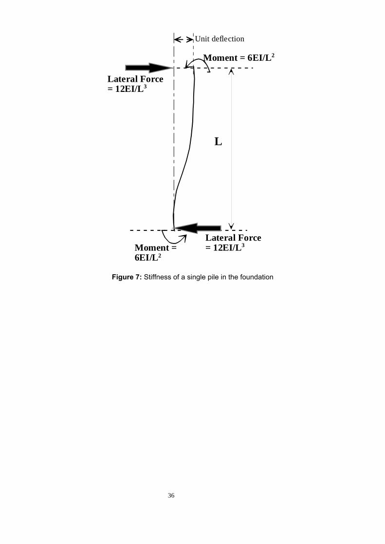
At the full liquefaction the base shear due to earthquake excitation will reduce. To estimate the base shear, it is necessary to predict the time period of vibration of the building for small vibrations when the soil surrounding the pile has liquefied. Considering the fixity at about 2m below the soft zone, it is considered reasonable to assume that the pile will be fixed at about 17 metres below the ground level. The stiffness of the building for small vibrations, at full liquefaction is approximated by equation 37. In the calculation, it is assumed that the stiffness of the piles contribute to the total stiffness of the pile-soil system. This assumption can be justified by the fact that the elastic stiffness of the liquefied soil is orders of magnitude less than the concrete pile. The model for estimating stiffness for a single pile is shown in Figure 7.

mMNm

MNmLEIk /3

1735.3212381238 33

2

3 =××

=×= (37)

The time period of the building during full liquefaction can therefore be estimated by equation 38.

smNsm

NkMT Liqa 5.4

/103)/8.9(10001565622 62, =

×××

== ππ (38),where

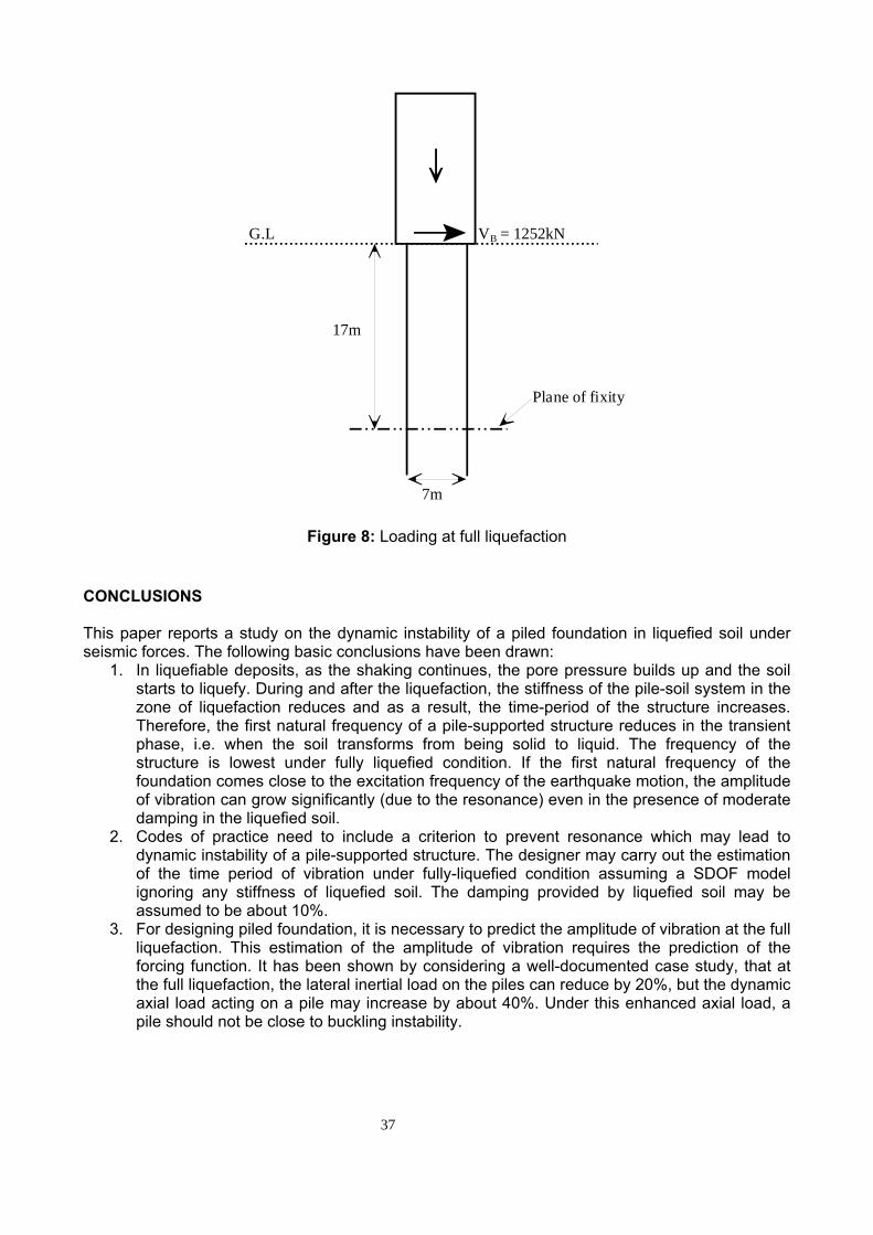
M = Mass of the building k = Stiffness of the building The calculation shows that the time period of vibration increases by 9 times and therefore the base shear in the building will decrease, following equations 28 and 30. It can immediately be inferred that the spectral acceleration will have decreased by a factor of 5 and therefore the base shear will reduce to 1252kN. Therefore, the increase in axial load on each pile is given by equation 39, following Figure 8.

kNm

kNmPinc 160197

171252=

××

= (39)

This is an increase of about 40%. Though the base shear has reduced by 5 times, it is the lever arm of the moment that has increased by about 7 times. The above calculations show that the axial load may increase by about 40% during the liquefaction stage.

Table 2: Design data of the building

Building height 14.5m above G.L Building dimensions 22.675m X 7m Foundation type Precast driven pile Building type R.C.C Framed Number of stories 5 Axial Load on each pile 412kN Dead load of the building 15656kN

Table 3: Design data of pile

Length 20 m External diameter 400mm Internal diameter 240mm Material Prestressed concrete E (Young’s Modulus) 30 GPa EI 32.35MNm2

Table 4: Values of the modulus of subgrade reaction

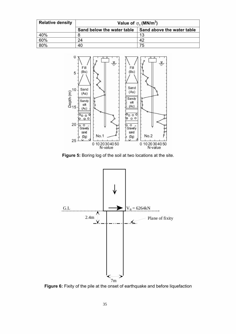
35

Value of hη (MN/m3) Relative density Sand below the water table Sand above the water table

40% 8 13 60% 24 42 80% 40 75

Figure 5: Boring log of the soil at two locations at the site.

VB = 6264kN

Plane of fixity

G.L

2.4m

7m Figure 6: Fixity of the pile at the onset of earthquake and before liquefaction

36

Moment = 6EI/L2

L

Moment =6EI/L2

Unit deflection

Lateral Force= 12EI/L3

Lateral Force= 12EI/L3

Figure 7: Stiffness of a single pile in the foundation

37

VB = 1252kN

Plane of fixity

G.L

17m

7m

Figure 8: Loading at full liquefaction

CONCLUSIONS This paper reports a study on the dynamic instability of a piled foundation in liquefied soil under seismic forces. The following basic conclusions have been drawn:

1. In liquefiable deposits, as the shaking continues, the pore pressure builds up and the soil starts to liquefy. During and after the liquefaction, the stiffness of the pile-soil system in the zone of liquefaction reduces and as a result, the time-period of the structure increases. Therefore, the first natural frequency of a pile-supported structure reduces in the transient phase, i.e. when the soil transforms from being solid to liquid. The frequency of the structure is lowest under fully liquefied condition. If the first natural frequency of the foundation comes close to the excitation frequency of the earthquake motion, the amplitude of vibration can grow significantly (due to the resonance) even in the presence of moderate damping in the liquefied soil.

2. Codes of practice need to include a criterion to prevent resonance which may lead to dynamic instability of a pile-supported structure. The designer may carry out the estimation of the time period of vibration under fully-liquefied condition assuming a SDOF model ignoring any stiffness of liquefied soil. The damping provided by liquefied soil may be assumed to be about 10%.

3. For designing piled foundation, it is necessary to predict the amplitude of vibration at the full liquefaction. This estimation of the amplitude of vibration requires the prediction of the forcing function. It has been shown by considering a well-documented case study, that at the full liquefaction, the lateral inertial load on the piles can reduce by 20%, but the dynamic axial load acting on a pile may increase by about 40%. Under this enhanced axial load, a pile should not be close to buckling instability.

38

REFERENCES: 1. AIJ (2001): Architectural Institute of Japan, Recommendations for design of building

foundations, (in Japanese). 2. API (2000): American Petroleum Institute, Recommended Practice for planning designing

and constructing Fixed offshore platforms – Load and Resistance Factor design. 3. Bhattacharya, S (2003): Pile Instability during earthquake liquefaction, PhD thesis,

University of Cambridge (U.K). 4. Bhattacharya, S. Madabhushi, S.P.G and Bolton, M.D (2004): “An alternative mechanism of

pile failure during seismic liquefaction”, Geotechnique 54, Issue 3 (April), pp 203-213. 5. Bhattacharya, S., Bolton, M.D and Madabhushi, S.P.G., (2005): “A reconsideration of the

safety of the piled bridge foundations in liquefiable soils”, Soils and Foundations, Vol 45, No 4, pp 13-26, August 2005 issue.

6. Davisson, M.T and Robertson, K.E. (1965): “Bending and buckling of partially embedded piles”. Proceedings of the 6th ICSMGE, Vol -2, pp 243-246.

7. Eurocode 7 (1997): Geotechnical Design, European Committee for standardization, Brussels.

8. EC 8: Eurocode 8 (Part 5, 1998): “Design provisions for earthquake resistance of structures-foundations, retaining structures and geotechnical aspects”, European Committee for Standardization, Brussels.

9. I.S: 1893(2002): Indian Standard Code of Practice for seismic design of structure. 10. JRA (2002): Japanese Road Association, Specification for Highway Bridges, Part V,

Seismic Design 11. Knappett and Madabhushi, S.P.G. (2005): “Modelling of Liquefaction-induced instability in

pile groups”. ASCE Special Publication No 145 on “Seismic Performance and Simulation of Pile Foundations in Liquefied and Laterally Spreading Ground”.

12. Leipholz, H. (1975): “Six Lectures on Stability of Elastic Systems” Solid Mechanics Division, University of Waterloo Press, Waterloo, Canada

13. Meyerhof, G.G (1957): Discussion, Proceedings of the 4th ICSMGE, Vol 3, pp 110. 14. NEHRP (2000): Commentary for FEMA (USA 369) on seismic regulations for new buildings

and other structures. 15. Takahashi, A., Kuwano, Y., and Yano, A. (2002): “Lateral resistance of buried cylinder in

liquefied sand”, Proceedings of the International Conference on physical modelling in geotechnics, ICPMG-02, St. John’s, Newfoundland, Canada, 10-12th July.

16. Towahata, I., Vargas-Mongem, W., Orense, R.P. and Yao, M (1999): “Shaking table tests on subgrade reaction of pipe embedded in sandy liquefied subsoil”, Soil Dynamics and Earthquake Engineering, Vol 18, No 5, pp 347-361.

17. Thomson, J.M.T and Hunt, G.W (1973): “A general theory of elastic stability”, Wiley, London

18. Timoshenko, S., Young, D.H. and Weaver, W. (1974): “Vibration problems in Engineering”, John Wiley and Sons. .

19. Uzuoka, R, Sento N, Yashima A. and Zhang F., (2002): “3-dimensional effective stress analysis of a damaged group-pile foundation adjacent to a quay wall”, Japanese Association for Earthquake Engineering (JAEE) Journal.

A Natural frequency for the pinned-pinned bound-

ary condition

Assuming harmonic solution (the separation of variable) we have

w(x, t) = W (ξ)exp iωt , ξ = x/L (A.1)

Substituting this in the equation of motion (4) and the boundary conditions in equations

(4a) – (4d) results

EI

L4

∂4W (ξ)

∂ξ4+

P

L2

∂2W (ξ)

∂ξ2+ k W (ξ)−mω2W (ξ) +

mr2ω2

L2

∂2W (ξ)

∂ξ2= 0 (A.2)

W (0) = 0 (A.3)

W ′′(0) = 0 (A.4)

W (L) = 0 (A.5)

W ′′(L) = 0 (A.6)

It is convenient to express equation of motion (A.2) in terms of non-dimensional param-

eters by elementary rearrangements as

∂4W (ξ)

∂ξ4+ ν

∂2W (ξ)

∂ξ2+ ηW (ξ)− Ω2W (ξ) = 0 (A.7)

where

ν = ν + µ2Ω2 (A.8)

and

ν =PL2

EI(nondimensional axial force) (A.9)

η =kL4

EI(nondimensional support stiffness) (A.10)

Ω2 = ω2mL4

EI(nondimensional frequency parameter) (A.11)

µ =r

L(nondimensional radius of gyration). (A.12)

It is often useful to express ν in terms of the critical buckling load as

ν = π2(P/Pcr) (A.13)

37

Because we are considering a pinned-pinned beam, the mode shapes are of the form

Wn(ξ) = sin(nπξ), n = 1, 2, 3, · · · (A.14)

Substituting this in the equation of motion (A.7) results

n4π4 − νn2π2 + η − Ω2n = 0 (A.15)

or n4π4 − (ν + Ω2nµ2)n2π2 + η − Ω2

n = 0 (A.16)

or Ω2n(1 + µ2n2π2) = n4π4 − νn2π2 + η (A.17)

or Ω2n =

n4π4

1 + µ2n2π2

(1− P/Pcr

n2+

η

n4π4

)(A.18)

This shows that the effective natural frequency reduces when the axial force increases.

B Derivation of the frequency equation for the gen-

eral case

The difference between this case and the pinned-pinned case discussed before arise only

due to the difference in the boundary conditions. Using the separation of variables in

equation (A.1), the boundary conditions in equations (9) – (12) can be transformed as

W (0) = 0 (B.1)

W ′(0) = 0 (B.2)

EI

L2W ′′(1)− ω2J

LW ′(1) = 0 (B.3)

EI

L3W ′′′(1) +

P

LW ′(1) + ω2M W (1) +

mr2ω2

LW ′(1) = 0 (B.4)

It is convenient to express these equations in terms of non-dimensional parameters by

elementary rearrangements as

W (0) = 0 (B.5)

W ′(0) = 0 (B.6)

W ′′(1)− βΩ2W ′(1) = 0 (B.7)

W ′′′(1) + νW ′(1) + αΩ2W (1) = 0 (B.8)

38

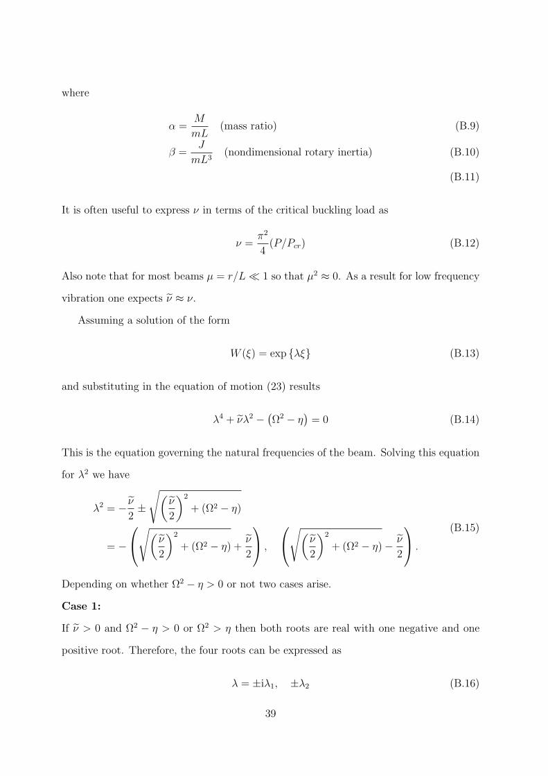
where

α =M

mL(mass ratio) (B.9)

β =J

mL3(nondimensional rotary inertia) (B.10)

(B.11)

It is often useful to express ν in terms of the critical buckling load as

ν =π2

4(P/Pcr) (B.12)

Also note that for most beams µ = r/L ¿ 1 so that µ2 ≈ 0. As a result for low frequency

vibration one expects ν ≈ ν.

Assuming a solution of the form

W (ξ) = exp λξ (B.13)

and substituting in the equation of motion (23) results

λ4 + νλ2 − (Ω2 − η

)= 0 (B.14)

This is the equation governing the natural frequencies of the beam. Solving this equation

for λ2 we have

λ2 = − ν

2±

√(ν

2

)2

+ (Ω2 − η)

= −

√(ν

2

)2

+ (Ω2 − η) +ν

2

,

√(ν

2

)2

+ (Ω2 − η)− ν

2

.

(B.15)

Depending on whether Ω2 − η > 0 or not two cases arise.

Case 1:

If ν > 0 and Ω2 − η > 0 or Ω2 > η then both roots are real with one negative and one

positive root. Therefore, the four roots can be expressed as

λ = ±iλ1, ±λ2 (B.16)

39

where

λ1 =

√(ν

2

)2

+ (Ω2 − η) +ν

2

1/2

(B.17)

and λ2 =

√(ν

2

)2

+ (Ω2 − η)− ν

2

1/2

. (B.18)

From Eqs. (B.17) and (B.18) also note that

λ21 − λ2

2 = ν. (B.19)

In view of the roots in in Eq. (B.16) the solution W (ξ) can be expressed as

W (ξ) = a1 sin λ1ξ + a2 cos λ1ξ + a3 sinh λ2ξ + a4 cosh λ2ξ

or W (ξ) = sT (ξ)a(B.20)

where the vectors

s(ξ) = sin λ1ξ, cos λ1ξ, sinh λ2ξ, cosh λ2ξT (B.21)

and a = a1, a2, a3, a4T . (B.22)

Applying the boundary conditions in Eqs. (24) – (27) on the expression of W (ξ) in

(B.20) we have

Ra = 0 (B.23)

where the matrix

R =

s1(0) s2(0)s′1(0) s′2(0)

s′′1(1)− βΩ2s′1(1) s′′2(1)− βΩ2s′2(1)s′′′1 (1)− νs′1(1) + αΩ2s1(1) s′′′2 (1)− νs′2(1) + αΩ2s2(1)

s3(0) s4(0)s′3(0) s′4(0)

s′′3(1)− βΩ2s′3(1) s′′4(1)− βΩ2s′4(1)s′′′3 (1)− νs′3(1) + αΩ2s3(1) s′′′3 (1)− νs′3(1) + αΩ2s3(1)

(B.24)

40

Substituting functions sj(ξ), j = 1, · · · , 4 from Eq. (B.21) and simplifying we obtain

R =

0 1λ1 0

− sin (λ1) λ12 − Ω2β cos (λ1) λ1 − cos (λ1) λ1

2 + Ω2β sin (λ1) λ1

− cos (λ1) λ13 − ν cos (λ1) λ1 + Ω2α sin (λ1) sin (λ1) λ1

3 + ν sin (λ1) λ1 + Ω2α cos (λ1)

0 1λ2 0

sinh (λ2) λ22 − Ω2β cosh (λ2) λ2 cosh (λ2) λ2

2 − Ω2β sinh (λ2) λ2

cosh (λ2) λ23 − ν cosh (λ2) λ2 + Ω2α sinh (λ2) sinh (λ2) λ2

3 − ν sinh (λ2) λ2 + Ω2α cosh (λ2)

.

(B.25)

The constant vector in Eq. (B.23) cannot be zero. Therefore, the equation governing the

natural frequencies is given by

|R| = 0 (B.26)

This, upon simplification reduces to

(− sin (λ1) λ12λ2Ω

2 cosh (λ2) + λ1Ω2 cos (λ1) sinh (λ2) λ2

2 − Ω4β sin (λ1) λ12 sinh (λ2)

−Ω2 sin (λ1) cosh (λ2) λ23 + Ω4 sin (λ1) β sinh (λ2) λ2

2 + cos (λ1) λ13Ω2 sinh (λ2)

−2 λ1Ω4 cos (λ1) β cosh (λ2) λ2 + 2 Ω4λ2β λ1

)α +

(λ1λ2

3 − cos (λ1) λ1 cosh (λ2) λ23

−2 sin (λ1) λ12 sinh (λ2) λ2

2 − λ13λ2 + cos (λ1) λ1

3 cosh (λ2) λ2

)ν + λ1

5λ2 + λ1λ25

+ 2 cos (λ1) λ13 cosh (λ2) λ2

3 + sin (λ1) λ14 sinh (λ2) λ2

2 − sin (λ1) λ12 sinh (λ2) λ2

4

−sin (λ1) λ14Ω2β cosh (λ2) λ2−Ω2β sin (λ1) λ1

2 cosh (λ2) λ23−Ω2β cos (λ1) λ1 sinh (λ2) λ2

4

− cos (λ1) λ13Ω2β sinh (λ2) λ2

2 = 0. (B.27)

The natural frequencies can be obtained by solving Eq. (B.27) for Ω. Due to the com-

plexity of this transcendental equation it must be solved numerically.

Case 2:

If ν > 0 and Ω2 − η < 0 or Ω2 < η then both the roots are real and negative. Therefore,

all of the four roots can be expressed as

λ = ±iλ1, ±iλ2 (B.28)

41

where λ1 is as in the previous case

λ1 =

ν

2+

√(ν

2

)2

− (η − Ω2)

1/2

(B.29)

and λ2 is given by

λ2 =

ν

2−

√(ν

2

)2

− (η − Ω2)

1/2

(B.30)

In view of the roots in in Eq. (B.28) the solution W (ξ) can be expressed as

W (ξ) = a1 sin λ1ξ + a2 cos λ1ξ + a3 sin λ2ξ + a4 cos λ2ξ

or W (ξ) = sT (ξ)a(B.31)

where the vectors

s(ξ) =

sin λ1ξ, cos λ1ξ, sin λ2ξ, cos λ2ξT

(B.32)

and a = a1, a2, a3, a4T . (B.33)

Applying the boundary conditions in Eqs. (B.5) – (B.8) on the expression of W (ξ) in

(B.31) and following similar procedure as the previous case, the frequency equation can

be expressed as

(cos (λ1) λ1 cos

(λ2

)λ3

2 − λ1λ32 − λ1

3λ2 + cos (λ1) λ13 cos

(λ2

)λ2 + 2 sin (λ1) λ1

2 sin(λ2

)λ2

2

)ν

+(−Ω4β sin (λ1) λ1

2 sin(λ2

)+ cos (λ1) λ1

3Ω2 sin(λ2

)− 2 λ1Ω

4 cos (λ1) β cos(λ2

)λ2 + 2 λ1Ω

4β λ2

−λ1Ω2 cos (λ1) sin

(λ2

)λ2

2 + Ω2 sin (λ1) cos(λ2

)λ3

2 − sin (λ1) λ12λ2Ω

2 cos(λ2

)

−Ω4 sin (λ1) β sin(λ2

)λ2

2

)α− 2 cos (λ1) λ1

3 cos(λ2

)λ3

2 − sin (λ1) λ14 sin

(λ2

)λ2

2

−sin (λ1) λ12 sin

(λ2

)λ4

2+λ15λ2−Ω2β cos (λ1) λ1 sin

(λ2

)λ4

2+Ω2β sin (λ1) λ12 cos

(λ2

)λ3

2

− sin (λ1) λ14Ω2β cos

(λ2

)λ2 + cos (λ1) λ1

3Ω2β sin (λ2) λ22 + λ1λ

52 = 0 (B.34)

The natural frequencies can be obtained by solving Eq. (B.34) for Ω. Due to the com-

plexity of this transcendental equation it must be solved numerically.

42