VIBRATION FATIGUE BROADBAND EXCITATION THE …adlandırılır. Yükleme statik olmaktan ziyade...
136
VIBRATION FATIGUE ANALYSIS OF STRUCTURES UNDER BROADBAND EXCITATION A THESIS SUBMITTED TO THE GRADUATE SCHOOL OF NATURAL AND APPLIED SCIENCES OF MIDDLE EAST TECHNICAL UNIVERSITY BY BİLGE KOÇER IN PARTIAL FULFILLMENT OF THE REQUIREMENTS FOR THE DEGREE OF MASTER OF SCIENCE IN MECHANICAL ENGINEERING JUNE 2010
Transcript of VIBRATION FATIGUE BROADBAND EXCITATION THE …adlandırılır. Yükleme statik olmaktan ziyade...
VIBRATION FATIGUE ANALYSIS OF STRUCTURES UNDER BROADBAND EXCITATION
A THESIS SUBMITTED TO THE GRADUATE SCHOOL OF NATURAL AND APPLIED SCIENCES
OF MIDDLE EAST TECHNICAL UNIVERSITY
BY
BİLGE KOÇER
IN PARTIAL FULFILLMENT OF THE REQUIREMENTS FOR
THE DEGREE OF MASTER OF SCIENCE IN
MECHANICAL ENGINEERING
JUNE 2010

ii
Approval of the thesis:
VIBRATION FATIGUE ANALYSIS OF STRUCTURES UNDER
BROADBAND EXCITATION submitted by BİLGE KOÇER in partial fulfillment of the requirements for the degree of Master of Science in Mechanical Engineering Department, Middle East Technical University by, Prof. Dr. Canan Özgen ________________ Dean, Graduate School of Natural and Applied Sciences Prof. Dr. Suha Oral ________________ Head of Department, Mechanical Engineering Assoc. Prof. Dr. Serkan Dağ ________________ Supervisor, Mechanical Engineering Dept., METU Asst. Prof. Dr. Yiğit Yazıcıoğlu ________________ Co‐Supervisor, Mechanical Engineering Dept., METU Examining Committee Members: Asst. Prof. Dr. Ergin Tönük _____________________ Mechanical Engineering Dept., METU Assoc. Prof. Dr. Serkan Dağ _____________________ Mechanical Engineering Dept., METU Asst. Prof. Dr. Yiğit Yazıcıoğlu _____________________ Mechanical Engineering Dept., METU Asst. Prof. Dr. Ender Ciğeroğlu _____________________ Mechanical Engineering Dept., METU Dr. Volkan Parlaktaş _____________________ Mechanical Engineering Dept., Hacettepe University
Date: 24 – 06 – 2010

iii
I hereby declare that all information in this document has been obtained and presented in accordance with academic rules and ethical conduct. I also declare that, as required by these rules and conduct, I have fully cited and referenced all material and results that are not original to this work.
Name, Last name : Bilge, Koçer
Signature :
iv
ABSTRACT
VIBRATION FATIGUE ANALYSIS OF STRUCTURES UNDER BROADBAND EXCITATION
Koçer, Bilge M.S., Department of Mechanical Engineering Supervisor: Assoc. Prof. Dr. Serkan Dağ Co‐Supervisor: Asst. Prof. Dr. Yiğit Yazıcıoğlu
June 2010, 117 pages
The behavior of structures is totally different when they are exposed to
fluctuating loading rather than static one which is a well known
phenomenon in engineering called fatigue. When the loading is not static
but dynamic, the dynamics of the structure should be taken into account
since there is a high possibility to excite the resonance frequencies of the
structure especially if the loading frequency has a wide bandwidth. In these
cases, the structure’s response to the loading will not be linear. Therefore, in
the analysis of such situations, frequency domain fatigue analysis
techniques are used which take the dynamic properties of the structure into
consideration. Vibration fatigue method is also fast, functional and easy to
implement.
In this thesis, vibration fatigue theory is examined. Throughout the research
conducted for this study, the ultimate aim is to find solutions to problems
arising from test application for the loadings with nonzero mean value
bringing a new perspective to mean stress correction techniques. A new

v
method is developed to generate a modified input loading history with a
zero mean value which leads in fatigue damage approximately equivalent
to damage induced by input loading with a nonzero mean value. A
mathematical procedure is proposed to implement mean stress correction
to the output stress power spectral density data and a modified input
loading power spectral density data is obtained. Furthermore, this method
is improved for multiaxial loading applications. A loading history power
spectral density set with zero mean but modified alternating stress, which
leads in fatigue damage approximately equivalent to the damage caused by
the unprocessed loading set with nonzero mean, is extracted taking all
stress components into account using full matrixes. The proposed
techniques’ efficiency is discussed throughout several case studies and
fatigue tests.
Keywords: Vibration Fatigue, Mean Stress Correction, Power Spectral
Density, Finite Element Method.
vi
ÖZ
YAPILARIN GENİŞ BANTLI TAHRİK ALTINDA TİTREŞİM KAYNAKLI YORULMA İNCELEMELERİ
Koçer, Bilge Yüksek Lisans, Makine Mühendisliği Bölümü Tez yöneticisi: Doç. Dr. Serkan Dağ Yardımcı tez yöneticisi: Yrd. Doç. Dr. Yiğit Yazıcıoğlu
Haziran 2010, 117 sayfa
Yapılar statik yükleme yerine dalgalanan bir yüklemeye maruz
kaldıklarında, davranışları tamamen değişiklik gösterir. Bu husus,
mühendislikte sıklıkla karşılaşılan bir durum olup yorulma olarak
adlandırılır. Yükleme statik olmaktan ziyade dinamik ise yapı dinamiği de
göz önünde bulundurulmalıdır çünkü özellikle yükleme frekans bandı
genişse yapının rezonans frekanslarını tahrik etme olasılığı yüksektir. Bu
tür durumlarda, yapının yüklemeye karşı tepkisi doğrusal olmayacaktır. Bu
yüzden, bu tarz problemlerin incelenmesinde, yapının dinamik özelliklerini
de dikkate alan frekans temelli yorulma analiz teknikleri kullanılır. Ayrıca,
titreşim kaynaklı yorulma yöntemi hızlı, kullanışlı ve uygulaması kolaydır.
Bu tezde, titreşim kaynaklı yorulma teorisi incelenmektedir. Bu çalışma için
gerçekleştirilen araştırma sürecinde esas amaç, ortalama değeri sıfırdan
farklı yüklemeler için test uygulamalarından kaynaklanan problemleri,
ortalama gerilme düzeltme tekniklerine yeni bir bakış açısı getirerek
çözmektir. Ortlaması sıfır olmayan bir girdi yükünün sebep olduğu
vii
yorulma hasarına yakın bir hasar meydana getirecek ve ortalaması sıfır
olacak şekilde modifiye edilmiş bir girdi yükü oluşturmak için yeni bir
yöntem geliştirilmiştir. Ortalama gerilme düzeltme formülünü çıktı gerilme
güç spektrum yoğunluk datasına uygulamak için matematiksel bir
prosedür önerilmiştir ve modifiye edilmiş girdi yükleme güç spektrum
yoğunluk datası elde edilmiştir. Ayrıca bu yöntem, çok yönlü yükleme
uygulamaları için de kullanılacak şekilde geliştirilmiştir. Ortalaması sıfır
olmayan işlenmemiş girdi yükü setinin yarattığı yorulma hasarına yakın bir
hasar oluşturacak ve ortalaması sıfır olacak şekilde dalga değerleri
modifiye edilmiş bir yükleme güç spektrum yoğunluk seti bütün gerilme
elemanlarını dikkate alarak ve tüm matrisleri kullanarak elde edilmiştir.
Önerilen tekniklerin etkinliği çeşitli örnek çalışmalarla ve yorulma
testleriyle değerlendirilmiştir.
Anahtar kelimeler: Titreşim Kaynaklı Yorulma, Ortalama Gerilme
Düzeltmesi, Güç Spektrum Yoğunluk, Sonlu Eleman Metodu

viii
To my dear family,
with love and gratitude...

ix
ACKNOWLEDGEMENTS
I am very thankful to my thesis supervisors, Assoc. Prof. Dr. Serkan Dağ,
and Asst. Prof. Dr. Yiğit Yazıcıoğlu, whose valuable guidance, technical
support, and contributions throughout this study enabled me to complete
this thesis work successfully and gave me enthusiasm in developing new
techniques in scientific studies.
I am pleased to express my special thanks to my family for their endless
support and help, especially to my mother who supported me morally
throughout my life. I also heartily thank to my fiancé, and colleague,
Mehmet Ersin Yümer, with my deepest appreciation for his understanding,
encouragement and willing assistance.
I am also grateful to TÜBİTAK‐SAGE, especially to Structural Mechanics
Division, for their technical guidance in academic studies. I would like to
thank to Dr. A. Serkan Gözübüyük and Dr. Özge Şen who inspired me to
achieve new solutions to the problems arising from test applications. Also, I
sincerely thank to my colleagues Ahmet Akbulut and Harun Davut
Kendüzler for their help in manufacturing test equipments.
Lastly, I offer my regards to my colleagues and friends who supported me
in any respect during the completion of this thesis.
x
TABLE OF CONTENTS
ABSTRACT ............................................................................................................. iv
ÖZ ............................................................................................................................ vi
ACKNOWLEDGEMENTS ................................................................................... ix
TABLE OF CONTENTS ......................................................................................... x
LIST OF FIGURES ................................................................................................ xii
LIST OF TABLES ................................................................................................. xvi
LIST OF SYMBOLS ............................................................................................ xvii
CHAPTERS
1. INTRODUCTION ............................................................................................... 1
1.1 Metal Fatigue Damage ............................................................................ 1
1.1.1 Properties of Fatigue Failure ........................................................... 2
1.1.2 Major Fatigue Damage Accidents During In Service .................. 5
1.2 Scope of the Thesis .................................................................................. 9
1.3 Outline of the Thesis ............................................................................. 10
2. LITERATURE SURVEY ................................................................................... 13
2.1 Historical Overview of Fatigue ........................................................... 13
2.2 Background of Vibration Fatigue ........................................................ 16
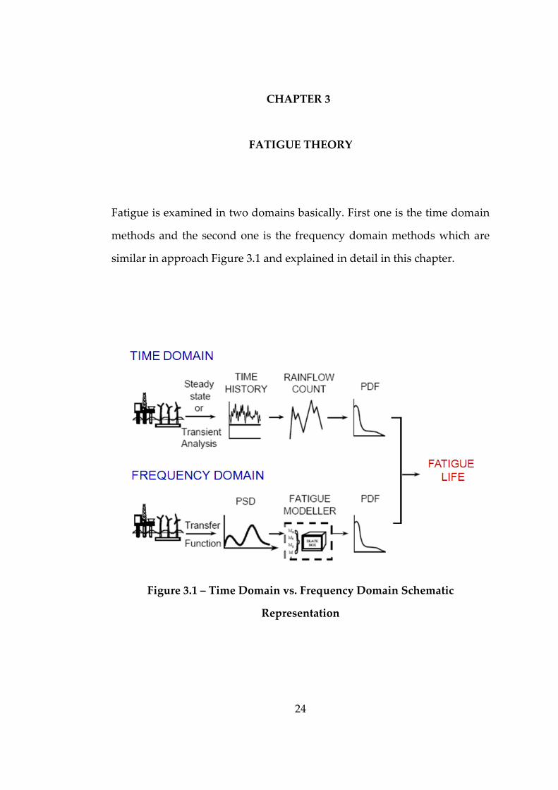
3. FATIGUE THEORY ......................................................................................... 24
3.1 Time Domain Fatigue Approaches ..................................................... 25
3.1.1 Stress Life (S‐N) Approach ............................................................ 25
3.1.2 Strain Life Approach ...................................................................... 37
3.1.3 Crack Propagation Approach ....................................................... 37
3.2 Frequency Domain Approach ............................................................. 37
3.2.1 Narrow Band Approach ................................................................ 48
xi
3.2.2 Empirical Correction Factors ........................................................ 50
3.2.3 Steinberg’s Solution........................................................................ 51
3.2.4 Dirlik’s Empirical Formulation .................................................... 52
4. A NEW METHOD FOR GENERATION OF A LOADING HISTORY
WITH ZERO MEAN ............................................................................................ 53
4.1 Theory ..................................................................................................... 55
4.2 Case Study .............................................................................................. 57
4.2.1 Finite Element Analyses ................................................................ 59
5. GENERATION OF A ZERO MEAN EXCITATION FOR MULTI‐AXIAL
LOADING .................................................................................................... 70
5.1 Theory ..................................................................................................... 71
5.2 Case Studies ........................................................................................... 74
5.2.1 Case Study I – Test Comparison .................................................. 74
5.2.2 Case Study II – Multi‐axial Loading ............................................ 90
6. CONCLUSIONS AND DISCUSSION ......................................................... 102
REFERENCES ..................................................................................................... 106
APPENDICES
A. TEST FIXTURE ............................................................................................... 113
B. COMPARISON OF SOLID AND SHELL FEM .......................................... 116
xii
LIST OF FIGURES
FIGURES
Figure 1.1 – Schematic section through a fatigue fracture showing the three
stages of crack propagation [4]. ............................................................................ 3
Figure 1.2 – Stage I: Crack Initiation .................................................................... 3
Figure 1.3 –A fatigue failure surface [52] ............................................................ 4
Figure 1.4 –Failure of a railway track component [52] ..................................... 5
Figure 1.5 – Lusaka Accident, 1977 [8] ................................................................ 6
Figure 1.6 – Chicago Accident, 1979: a) An amateur photo, as the aircraft
rolling past a 90° bank angle, b) explosion as the airplane impacts [9] .......... 7
Figure 1.7 – A Cracked Flange of American Airplane [8] ................................ 8
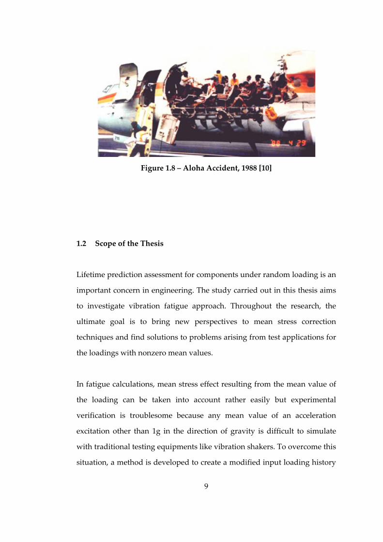
Figure 1.8 – Aloha Accident, 1988 [10] ................................................................ 9
Figure 1.9– Outline of the Thesis ........................................................................ 12
Figure 3.1 – Time Domain vs. Frequency Domain Schematic Representation
................................................................................................................................. 24
Figure 3.2 – Stress Cycles; (a) fully reversed, (b) offset ................................... 26
Figure 3.3 – Standard form of the material S‐N curve [52] ............................ 27
Figure 3.4 – S‐N curves for ferrous and non‐ferrous metals [52] .................. 28
Figure 3.5 ‐ Mean Stress Modification Methods [1] ......................................... 31
Figure 3.6 – Block Loading Sequence ................................................................ 33
Figure 3.7 – Broadband Random Loading ........................................................ 34
Figure 3.8 – Rainflow Cycles [52] ....................................................................... 35
Figure 3.9 – Rainflow Counting Example: a) Time History b) Reduced
History c) Rainflow Count [52] .......................................................................... 36
Figure 3.10 – Fourier Transformation ................................................................ 40
xiii
Figure 3.11 – Schematic Representation of Power Spectral Density ............. 41
Figure 3.12 – Time Histories and PSDs ............................................................. 42
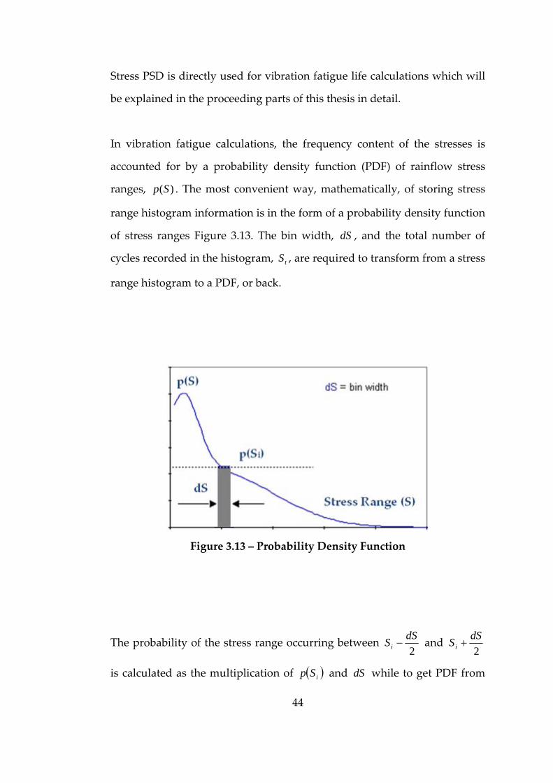
Figure 3.13 – Probability Density Function ...................................................... 44
Figure 3.14 – PSD Moments Calculation ........................................................... 47
Figure 3.15 – Expected Zeros and Expected Peaks in the Time History ...... 47
Figure 3.16 – Narrow Band Solution ................................................................. 49
Figure 4.1 – Plate Subjected to Base Excitation ................................................ 55
Figure 4.2 – Input Acceleration Loading Time History .................................. 58
Figure 4.3 – Input Acceleration Loading PSD .................................................. 59
Figure 4.4 – First Mode Shape (1st Bending) of the Cantilever Beam ............ 60
Figure 4.5 – Second Mode Shape (1st Torsion) of the Cantilever Beam ........ 60
Figure 4.6 – Third Mode Shape (2nd Bending) of the Cantilever Beam ......... 61
Figure 4.7 – Fourth Mode Shape (2nd Torsion) of the Cantilever Beam ........ 61
Figure 4.8 – Fifth Mode Shape (3rd Bending) of the Cantilever Beam ........... 62
Figure 4.9 – Frequency Response Analysis Results of the Cantilever Plate
for First Five Natural Frequencies for node 511 (Logarithmic Scale) ........... 63
Figure 4.10 – Load and Boundary Conditions of Static Analysis .................. 64
Figure 4.11 – Static von Mises Stress on the Cantilever Plate ........................ 64
Figure 4.12 – Modified Input Loading and Original Input Loading for
Cantilever Plate ..................................................................................................... 66
Figure 4.13 – Fatigue Life for the Plate (in seconds): a) without Mean Stress
Correction. ............................................................................................................. 66
Figure 4.14 – Finite Element Model of Displaying the Plate‐Node Numbers
................................................................................................................................. 68
Figure 5.1 – Dimensions of the test specimen (Dimensions in [mm]) .......... 74
Figure 5.2 – Vertical test configuration ............................................................. 76
Figure 5.3 – Horizontal test configuration ........................................................ 76
xiv
Figure 5.4 – Acceleration Input PSD .................................................................. 77
Figure 5.5 – Original and corrected acceleration input PSDs ........................ 78
Figure 5.6 – Difference between corrected and original acceleration input
PSDs (Corrected ‐ Original) ................................................................................ 78
Figure 5.7 – Finite element model ...................................................................... 79
Figure 5.8 – Fatigue life for the plate: without mean stress correction ......... 80
Figure 5.9 – Fatigue life for the plate: without mean stress correction (close‐
up) ........................................................................................................................... 80
Figure 5.10 – Fatigue life for the plate: with mean stress correction ............. 81
Figure 5.11 – Fatigue life for the plate: with mean stress correction (close‐
up) ........................................................................................................................... 81
Figure 5.12 – Fatigue life for the plate: with mean stress correction via
proposed method ................................................................................................. 82
Figure 5.13 – Fatigue life for the plate: with mean stress correction via
proposed method (close‐up) ............................................................................... 82
Figure 5.14 – Fatigue life for the plate: without mean stress correction
(close‐up, logarithmic scale) ............................................................................... 84
Figure 5.15 – Fatigue life for the plate: with mean stress correction (close‐
up, logarithmic scale) ........................................................................................... 84
Figure 5.16 – Fatigue life for the plate: with proposed method (close‐up,
logarithmic scale) .................................................................................................. 85
Figure 5.17 – Damaged specimen 1: without mean stress .............................. 87
Figure 5.18 – Damaged specimen 1: without mean stress (close‐up) .......... 87
Figure 5.19 – Damaged specimen 2: with mean stress .................................... 88
Figure 5.20 – Damaged specimen 2: with mean stress (close‐up) ................. 88
Figure 5.21 – Damaged specimen 3: with proposed method ......................... 89
Figure 5.22 – Damaged specimen 3: with proposed method (close‐up) ...... 89
xv
Figure 5.23 – Fin type aerodynamic surface ..................................................... 91
Figure 5.24 – FEM of the fin type aerodynamic surface ................................. 92
Figure 5.25 – Input time history in x‐axis ......................................................... 92
Figure 5.26 – Input PSD in x‐axis ....................................................................... 93
Figure 5.27 – Input time history in y‐axis ......................................................... 93
Figure 5.28 – Input PSD in y‐axis ....................................................................... 94
Figure 5.29 – Input time history in z‐axis ......................................................... 94
Figure 5.30 – Input PSD in z‐axis ....................................................................... 95
Figure 5.31 – Corrected and Original Input PSDs in x‐axis ........................... 96
Figure 5.32 – Corrected and Original Input PSDs in y‐axis ........................... 96
Figure 5.33 – Corrected and Original Input PSDs in z‐axis ........................... 97
Figure 5.34 – Fatigue life for the fin: without mean stress correction ........... 98
Figure 5.35 – Fatigue life for the fin: with mean stress correction................. 98
Figure 5.36 – Fatigue life for the fin: corrected with the proposed method 99
Figure 5.37 – Fatigue life for the fin: without mean stress correction (close‐
up) ........................................................................................................................... 99
Figure 5.38 – Fatigue life for the fin: with mean stress correction (close‐up)
............................................................................................................................... 100
Figure 5.39 – Fatigue life for the fin: with the proposed method (close‐up)
............................................................................................................................... 100
Figure A.1 – Test Fixture ................................................................................... 113
Figure A.2 – Test Fixture – Specimen Assembly Types ................................ 114
Figure A.3 – First Mode Shape of the Test Fixture ........................................ 114
Figure A.4 – Second Mode Shape of the Test Fixture ................................... 115
Figure A.5 – Third Mode Shape of the Test Fixture ...................................... 115
Figure B.1 – Plate Dimensions ........................................................................... 116
xvi
LIST OF TABLES
TABLES
Table 4.1 – Dimensions of the Plate ................................................................... 55
Table 4.2 – Comparisons of Fatigue Life Values .............................................. 68
Table 5.1 – Input PSD Data ................................................................................. 77
Table 5.2 – Life values from analysis ................................................................. 83
Table 5.3 – Life values from tests ....................................................................... 86
Table 5.4 – Mean value of life from tests ........................................................... 86
Table 5.5 – Comparison of life values from test and analysis ........................ 90
Table B.1 – Constant A for a/b=5 ....................................................................... 116
Table B.2 – Natural Frequencies Errors ............................................................ 117

xvii
LIST OF SYMBOLS
S : Stress
nN , : Number of cycles
a : Crack size
aS : Alternating stress amplitude
rS : Stress range
mS : Mean stress
maxS : Maximum stress amplitude
minS : Minimum stress amplitude
R : Stress ratio
b : Basquin exponent
C : Material constant
oS : Fatigue limit
eS : Endurance limit
iK : Stress concentration factor
fK : Fatigue strength concentration factor
q : Notch Sensitivity
ak : Surface condition modification factor
bk : Size modification factor
ck : Load modification factor
dk : Temperature modification factor
ek : Reliability factor
fk : Miscellaneous‐effects modification factor
xviii
'eS : Laboratory test specimen endurance limit
aS : Alternating stress
'aS : Equivalent alternating stress
mS : Mean stress
uS : Ultimate tensile strength
yS : Tensile yield strength
[ ]DE : Expected damage
PSD : Power spectral density
pT : Period
)(ty : Time history
nno BAA ,, : Fourier coefficients
PSD : Power spectral density
)( fy : Frequency spectrum of time history
FFT : Fast Fourier Transform
IFFT : Inverse Fourier Transform
)( fH : Transfer function
)(* fH : Complex conjugate of transfer function
)( fGr : Response stress PSD
)( fGi : Input acceleration PSD
)(Sp : Probability density function (PDF) of rainflow stress ranges
nm : The nth spectral moment of the PSD of stress
)(PE : Expected number of peaks per second
)0(E : Expected number of upward zero crossings per second
γ : Irregularity factor
)( fGrm : Modified output stress PSD

xix
)( fGim : Modified input acceleration PSD
{ })( fσ : Output stress vector
{ })( fa : Input acceleration vector
{ })( fmσ : Modified output stress vector
[ ])( fGmσ : Modified output stress PSD matrix
[ ])( fGma : Modified input acceleration PSD matrix
1
CHAPTER 1
INTRODUCTION
The aerospace industry’s increasing demands for durability, safety,
reliability, long life and low cost lead in high interest in studies for
improving strength, quality, productivity, and longevity of components in
engineering science. Consequently, these products should be designed and
tested for sufficient fatigue resistance over a desired range of product
populations to satisfy the needs.
1.1 Metal Fatigue Damage
The behavior of machine parts becomes totally different when they are
subjected to fluctuating loading rather than static one. Often, machine
members fail under the excitation of repeated or alternating stresses; yet the
most careful analysis shows that the actual maximum stresses are well
below the ultimate strength of the material, and quite frequently even
below the yield strength. The most distinguishing characteristic of these
failures is that the stresses repeat in a cyclic manner very large number of
times. Such a failure is called a fatigue failure [1]. In other words, metal
fatigue is the progressive and localized structural damage that occurs when
a material is subjected to alternating, cyclic, varying loading.
2
1.1.1 Properties of Fatigue Failure
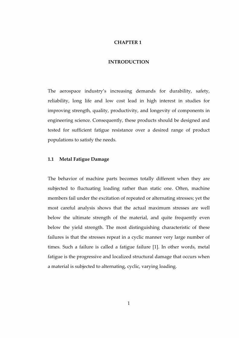
A fatigue failure looks like a brittle fracture, since the fracture surfaces are
flat and perpendicular to the stress axis without necking occurring.
However, fracture characteristics of fatigue failure are quite different from
the static brittle fracture in the aspect that fatigue failure comes out in
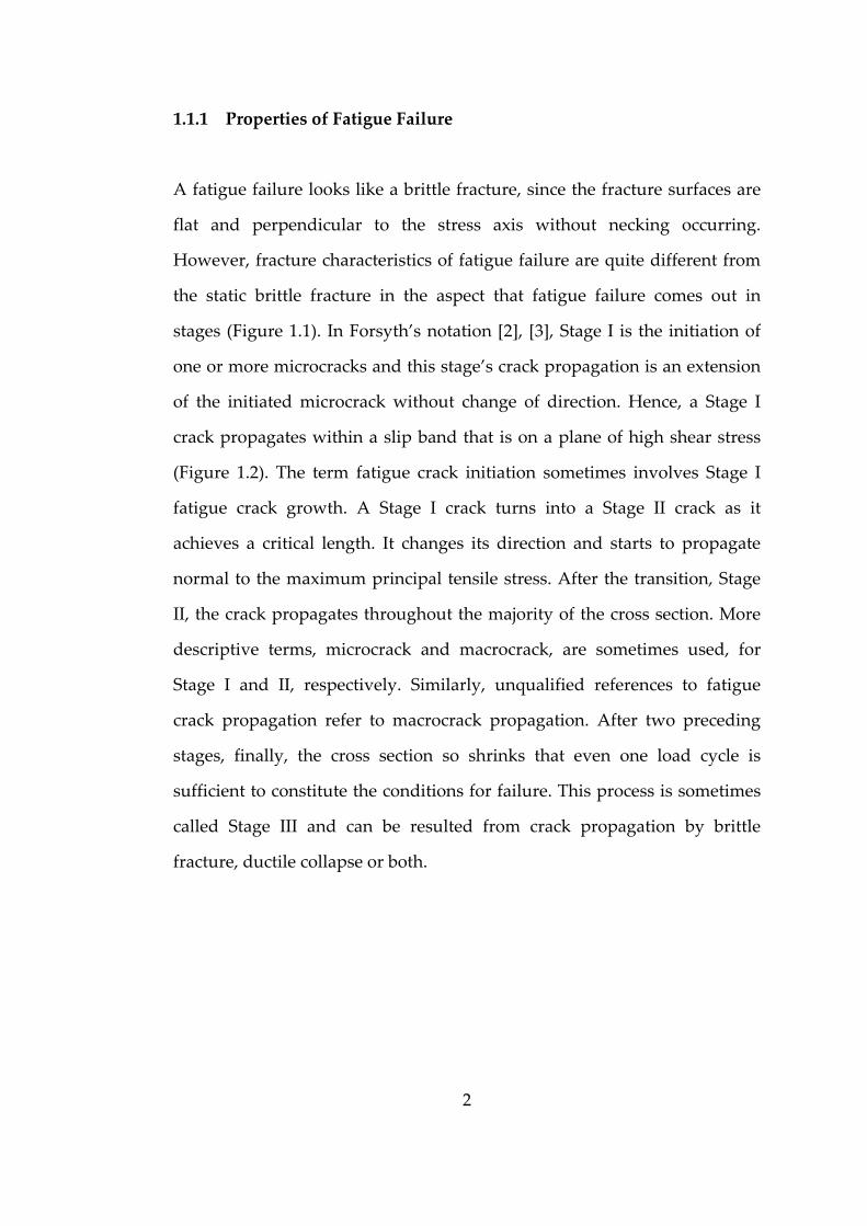
stages (Figure 1.1). In Forsyth’s notation [2], [3], Stage I is the initiation of
one or more microcracks and this stage’s crack propagation is an extension
of the initiated microcrack without change of direction. Hence, a Stage I
crack propagates within a slip band that is on a plane of high shear stress
(Figure 1.2). The term fatigue crack initiation sometimes involves Stage I
fatigue crack growth. A Stage I crack turns into a Stage II crack as it
achieves a critical length. It changes its direction and starts to propagate
normal to the maximum principal tensile stress. After the transition, Stage
II, the crack propagates throughout the majority of the cross section. More
descriptive terms, microcrack and macrocrack, are sometimes used, for
Stage I and II, respectively. Similarly, unqualified references to fatigue
crack propagation refer to macrocrack propagation. After two preceding
stages, finally, the cross section so shrinks that even one load cycle is
sufficient to constitute the conditions for failure. This process is sometimes
called Stage III and can be resulted from crack propagation by brittle
fracture, ductile collapse or both.
3
Figure 1.1 – Schematic section through a fatigue fracture showing the
three stages of crack propagation [4].
Figure 1.2 – Stage I: Crack Initiation
4
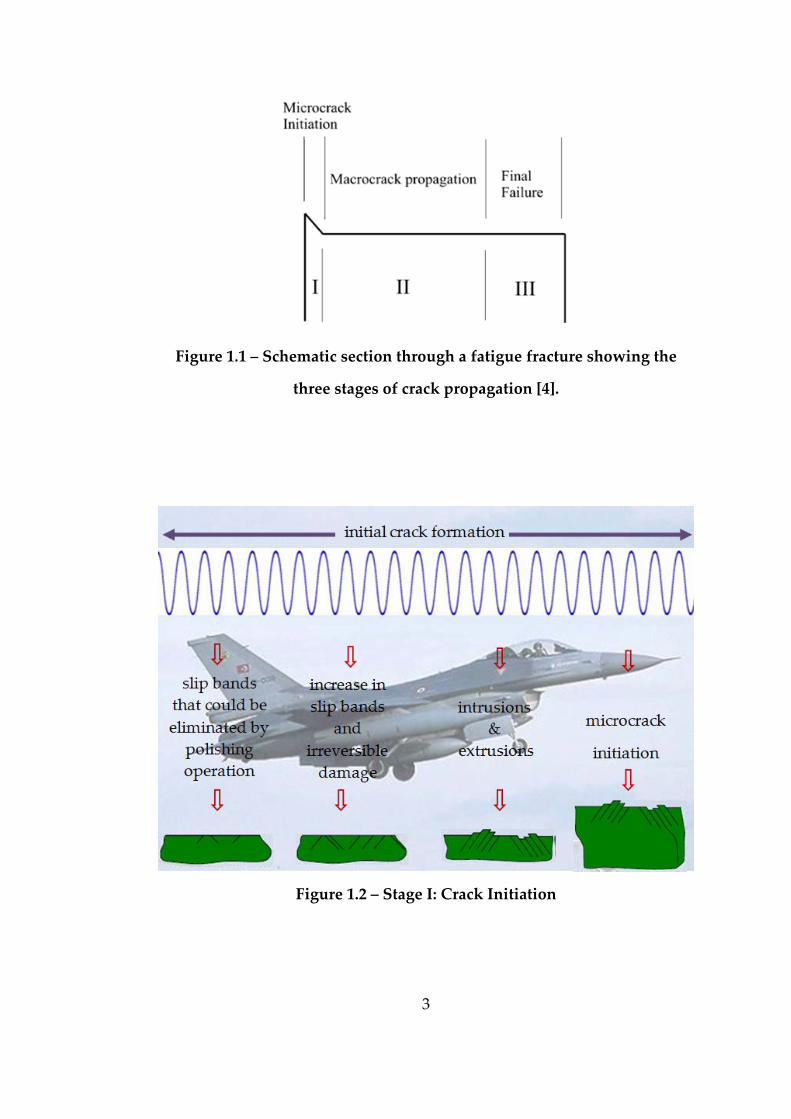
Most of the static failures give a visible warning in advance, such as
developing a large deflection due to the exceeding of yield strength of the
material, before the total fracture occurs. However, fatigue failures are
sudden and total usually without a warning, therefore dangerous. Figure
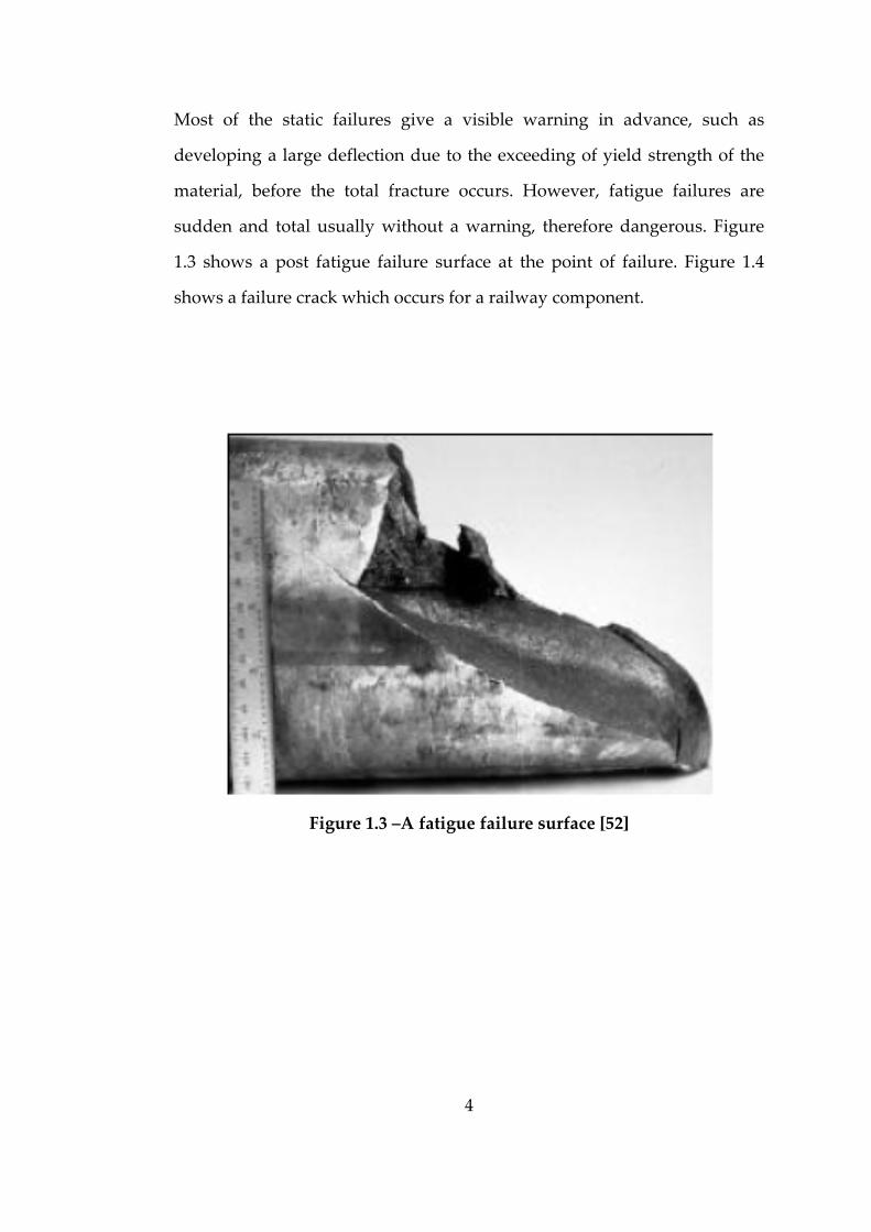
1.3 shows a post fatigue failure surface at the point of failure. Figure 1.4
shows a failure crack which occurs for a railway component.
Figure 1.3 –A fatigue failure surface [52]
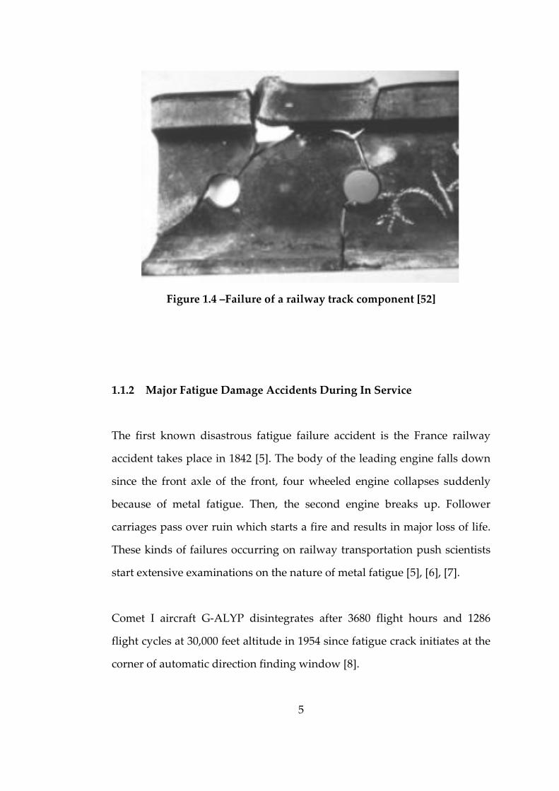
5
Figure 1.4 –Failure of a railway track component [52]
1.1.2 Major Fatigue Damage Accidents During In Service
The first known disastrous fatigue failure accident is the France railway
accident takes place in 1842 [5]. The body of the leading engine falls down
since the front axle of the front, four wheeled engine collapses suddenly
because of metal fatigue. Then, the second engine breaks up. Follower
carriages pass over ruin which starts a fire and results in major loss of life.
These kinds of failures occurring on railway transportation push scientists
start extensive examinations on the nature of metal fatigue [5], [6], [7].
Comet I aircraft G‐ALYP disintegrates after 3680 flight hours and 1286
flight cycles at 30,000 feet altitude in 1954 since fatigue crack initiates at the
corner of automatic direction finding window [8].
6
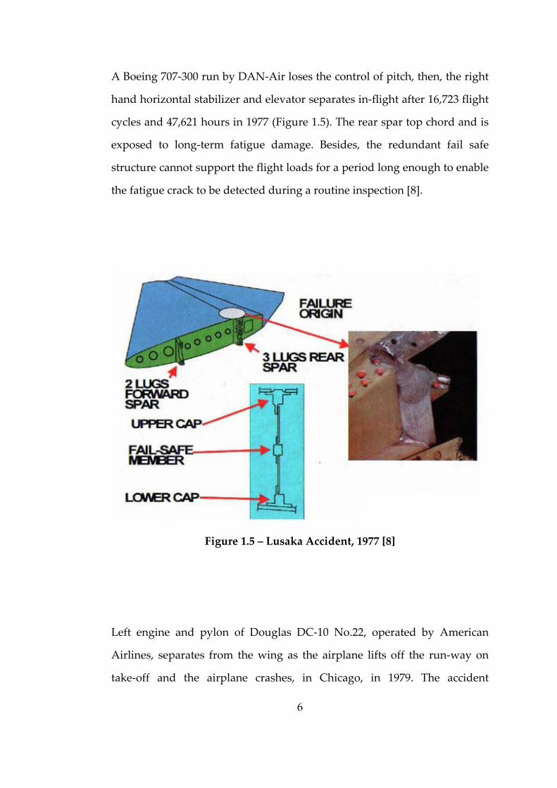
A Boeing 707‐300 run by DAN‐Air loses the control of pitch, then, the right
hand horizontal stabilizer and elevator separates in‐flight after 16,723 flight
cycles and 47,621 hours in 1977 (Figure 1.5). The rear spar top chord and is
exposed to long‐term fatigue damage. Besides, the redundant fail safe
structure cannot support the flight loads for a period long enough to enable
the fatigue crack to be detected during a routine inspection [8].
Figure 1.5 – Lusaka Accident, 1977 [8]
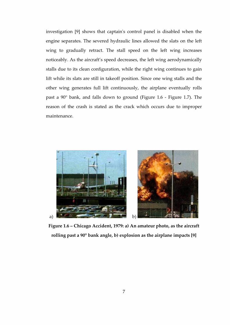
Left engine and pylon of Douglas DC‐10 No.22, operated by American
Airlines, separates from the wing as the airplane lifts off the run‐way on
take‐off and the airplane crashes, in Chicago, in 1979. The accident
7
investigation [9] shows that captainʹs control panel is disabled when the
engine separates. The severed hydraulic lines allowed the slats on the left
wing to gradually retract. The stall speed on the left wing increases
noticeably. As the aircraft’s speed decreases, the left wing aerodynamically
stalls due to its clean configuration, while the right wing continues to gain
lift while its slats are still in takeoff position. Since one wing stalls and the
other wing generates full lift continuously, the airplane eventually rolls
past a 90° bank, and falls down to ground (Figure 1.6 ‐ Figure 1.7). The
reason of the crash is stated as the crack which occurs due to improper
maintenance.
a) b)
Figure 1.6 – Chicago Accident, 1979: a) An amateur photo, as the aircraft
rolling past a 90° bank angle, b) explosion as the airplane impacts [9]
8
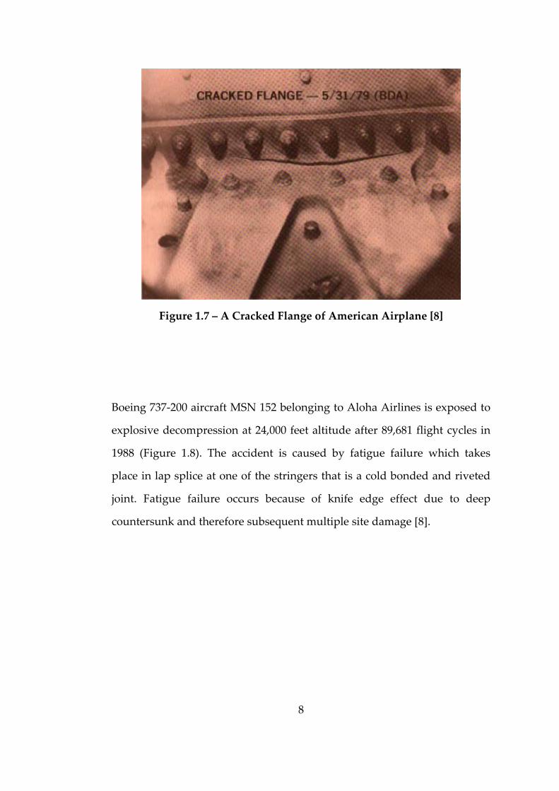
Figure 1.7 – A Cracked Flange of American Airplane [8]
Boeing 737‐200 aircraft MSN 152 belonging to Aloha Airlines is exposed to
explosive decompression at 24,000 feet altitude after 89,681 flight cycles in
1988 (Figure 1.8). The accident is caused by fatigue failure which takes
place in lap splice at one of the stringers that is a cold bonded and riveted
joint. Fatigue failure occurs because of knife edge effect due to deep
countersunk and therefore subsequent multiple site damage [8].
9
Figure 1.8 – Aloha Accident, 1988 [10]
1.2 Scope of the Thesis
Lifetime prediction assessment for components under random loading is an
important concern in engineering. The study carried out in this thesis aims
to investigate vibration fatigue approach. Throughout the research, the
ultimate goal is to bring new perspectives to mean stress correction
techniques and find solutions to problems arising from test applications for
the loadings with nonzero mean values.
In fatigue calculations, mean stress effect resulting from the mean value of
the loading can be taken into account rather easily but experimental
verification is troublesome because any mean value of an acceleration
excitation other than 1g in the direction of gravity is difficult to simulate
with traditional testing equipments like vibration shakers. To overcome this
situation, a method is developed to create a modified input loading history
10
with a zero mean which causes fatigue damage approximately equivalent
to that created by input loading with a nonzero mean. A mathematical
procedure is proposed to implement mean stress correction to the output
von Mises stress power spectral density data. Furthermore, this method is
extended to generate a loading history set in multi‐axis with zero mean but
modified alternating stress, which leads in fatigue damage approximately
equivalent to the damage caused by the unprocessed loading set with
nonzero mean, taking all stress components into account using full
matrices. The efficiency of proposed solutions is discussed throughout
several case studies and fatigue tests.
1.3 Outline of the Thesis
Chapter 1 begins with preliminary information on fatigue definition, metal
fatigue mechanism, fatigue failure and the importance of design
considering fatigue criterion illustrating major fatigue accidents during
service.
In Chapter 2, the emphasis is on literature survey. Historical overview of
fatigue theory with the milestones of the fatigue phenomenon is presented
in this chapter in a chronological order. Furthermore, a subchapter is
completely separated to investigate the progress in vibration fatigue
approach mentioning the research and studies carried out in this field.
Chapter 3 is devoted to fatigue theory. Time domain methods and
frequency domain methods are discussed. Stress life approach is examined
in detail where mean stress effects on fatigue life and counting methods are

11
presented. Besides, stress life approach and crack propagation approach are
mentioned briefly. Moreover, frequency domain vibration fatigue theory is
examined in detail where narrowband solutions and wideband solutions
are discussed.
In Chapter 4, a new method for generation of a loading history with zero
mean is proposed, whose efficiency is discussed throughout a case study.
The method aims to obtain zero mean loading for a structure,
approximately equivalent in fatigue damage that is subjected to random
loading with nonzero mean making use of the frequency domain fatigue
calculation techniques and output stress power spectral density.
Chapter 5 is dedicated to the extension of the technique proposed in
Chapter 4. The goal is to generate a loading history with zero mean for
multiaxial loading. A multiaxial input loading with zero mean but
modified alternating stress, which creates fatigue damage approximately
equivalent to the damage caused by the unprocessed loading set with
nonzero mean, is extracted by means of the frequency domain fatigue
calculation techniques and output stress power spectral density. The
efficiency of proposed approach is discussed throughout case studies and
fatigue tests.
Finally, Chapter 6 summarizes the work done throughout the research, and
evaluates the outcomes and contributions to the literature.
Schematic representation of the thesis outline is given in Figure 1.9.
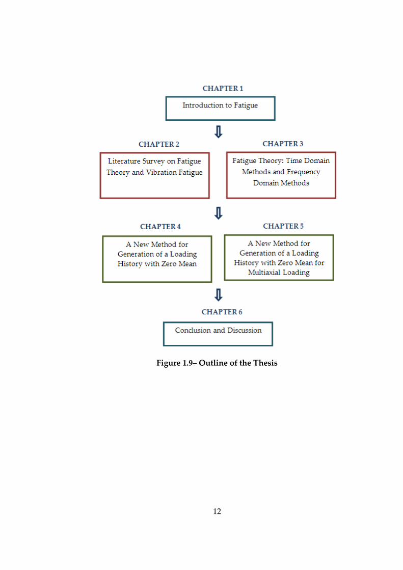
12
Figure 1.9– Outline of the Thesis
13
CHAPTER 2
LITERATURE SURVEY
2.1 Historical Overview of Fatigue
The first fatigue examinations seems to have been reported by Albert, a
mining engineer, who carried out some repeated loading tests on iron chain
in 1829 [11].
As railway service started to improve rapidly throughout the nineteenth
century, fatigue failures of railway axles become a widespread problem.
This situation requires that the cyclic loading effect should be taken into
consideration. The first major impact of failures resulting from repeated
stresses appears in the railway industry in the 1840s. It is recognized that
railroad axles fails regularly at shoulders [12]. Then, the removal of sharp
corners is recommended.
The term “fatigue” is introduced to explain failures happening due to
alternating stresses in the 1840s and 1850s. The first usage of the word
“fatigue” in print comes into view by Braithwaite, although Braithwaite
states in his paper that it is coined by Mr. Field [13]. Then, a general opinion
starts to develop in such a way that the material gets tired of bearing the
load or repeating application of a load exhausts the capability of the
material to carry load which survives to this day [4].
14
August Wöhler, a German railway engineer, sets and performs the first
systematic fatigue examination from 1852 to 1870. He carries out
experiments on full‐scale railway axles and also on small scale torsion,
bending, and axial cyclic loading test specimens for different materials.
Wöhler’s data for Krupp axle steel are plotted as nominal stress amplitude
versus cycles to failure. This presentation of fatigue life leads in the S‐N
diagram. Furthermore, Wöhler indicates that the range of stress is more
important than the maximum stress for fatigue failure [11], [14].
Gerber, Goodman and some other researchers examine the influence of
mean stress in loading throughout 1870s and 1890s.
Bauschinger [15] points out that the yield strength in compression or
tension decreases after applying a load of the opposite sign that results in
inelastic deformation. It is the first indication that a single exchange of
inelastic strain could alter the stress‐strain behavior of metals.
Ewing and Humfrey [16] study on fatigue mechanisms in microscopic scale
observing microcracks in the early 1900s. Basquin [17] represents
alternating stress versus number of cycles to failure (S‐N) in the finite life
region as a log‐log linear correlation in 1910.
Grififth [18], an important contributor to fracture mechanics, presents
theoretical calculations and experiments on brittle fracture by means of
glass in the 1920s. He states that the relation aS = constant, where S is the
nominal stress at fracture and a is the crack size at fracture.

15
Palmgren [19] introduces a linear cumulative damage model for loading
with varying amplitude in 1924. Neuber [20] demonstrates stress gradient
effects at notches in the 1930s. Miner [21] formulates linear cumulative
fatigue damage criterion proposed by Palmgren in 1945 which is now
known as Palmgren‐Miner linear damage rule.
Irwin [22] introduces the stress intensity factor KI, which is known as the
basis of linear elastic fracture mechanics and the origin of fatigue crack
growth life calculations. The Weibull distribution [23] grants a two‐
parameter and a three‐parameter statistical distribution for probabilistic
fatigue life analysis and testing.
Manson‐Coffin relationship [24][25] investigates the relationship between
plastic strain amplitude at the crack tip and fatigue life. The idea is
developed by Morrow [26]. Matsuishi and Endo [27] formulate the
rainflow‐counting algorithm to determine stress ranges for variable
amplitude loading.
Elber [28] develops a quantitative model which figures crack closure on
fatigue crack growth in 1970. Paris [29] shows that a threshold stress
intensity factor could be obtained for which fatigue crack growth would not
occur in 1970.
Throughout the 1980s and the 1990s, many researchers study on the
complex problem of in phase and out‐of‐phase multi‐axial fatigue, critical
plane models are proposed.

16
2.2 Background of Vibration Fatigue
Rice [30] develops the very important relationships for the number of
upward mean crossings per second and peaks per second in a random
signal expressed solely in terms of their spectral moments of the power
spectral density of the signal. This is the first serious effort at providing a
solution for estimating fatigue damage from power spectral density.
Bendat [31] presents the theoretical basis for the so‐called Narrow Band
solution. The expression used for the estimation of expected value of
damage is defined only in terms of the spectral moments of the power
spectral density up to the fourth degree.
Many expressions are proposed to improve narrow band solution [31] and
adapt it to broad band type. Most of them are developed with regards to
offshore platform design where interest in the techniques has existed for
many years. The methods are produced by generating sample time histories
from power spectral densities using Inverse Fourier Transform techniques.
Then probability density function of stress ranges is estimated empirically.
The solutions of Wirsching et al. [32], Chaudhury and Dover [33], Tunna
[34], Hancock [35], and Kam and Dover [35] formulas are all derived using
mentioned technique. They are all expressed in terms of the spectral
moments of power spectral density up to the fourth degree.
Steinberg [36] presents three band technique, based on Gaussian
distribution, for fatigue failure under random vibration for electronic
components. It is a simplified approach which does not require a large

17
computational effort. Therefore it is valuable as a time saving method. The
proposed method is based on a large volume of test data that was arranged
and rearranged to verify that a simplification in determining stress ranges
distribution is usable to analyze random vibration fatigue failures with
reasonable accuracy.
Dirlik [37] develops an empirical closed form expression for determination
of the probability density function of rainflow ranges directly from power
spectral density. The solution is obtained using extensive computer
simulations to model the signals using the Monte Carlo technique.
Wu et al. [38] work on a group of specimens made of 7075‐T651 aluminum
alloy to examine the applicability of methods proposed in the estimation of
fatigue damage and fatigue life of components under random loading.
Fatigue test results illustrate that the fatigue damage estimated based on
the Palmgren‐Miner rule can be improved by applying Morrow’s plastic
work interaction damage rule. Furthermore, random vibration theory for
narrow band process is utilized to estimate fatigue life where the
probability density function of the stress amplitudes is determined by
means of Rayleigh distribution for a zero‐mean narrow‐band Gaussian
random process.
Bishop et al. [39] present a state of the art perspective of random vibration
fatigue technology. Several design applications are presented. Time and
frequency domain methods are investigated and compared performing
finite element analysis using a model of a bracket, which is fully fixed at the
position of a round hole inside. Time domain and frequency domain
18
calculations show agreement if a transient dynamic analysis is carried out
with time domain fatigue life calculations for the excitations whose
frequency range includes the natural frequencies of the specimen. Also, it is
stated that the time and frequency domain processes are actually very
similar. The only differences are the structural analysis approach used (time
or frequency domain) and the fact that a fatigue modeler is needed as a tool
to extract the rainflow cycle histogram from the PSD of stress.
Liou et al. [40] study the theory of random vibration which is incorporated
into the calculation of the fatigue damage of the component subjected to
variable amplitude loading making use of the fundamental stress‐life cycle
relationship and different accumulation rules. The purpose is to derive
ready to‐use formulas for the prediction of fatigue damage and fatigue life
when a component is subjected to statistically defined random stresses.
Morrowʹs plastic work interaction damage rule is considered, in particular,
in the derivation in which the maximum stress peak should be taken into
consideration and it gives rather accurate fatigue life prediction in the long
life region and slightly conservative life in the short life region with the use
of Miner’s rule. Moreover, a series of fatigue tests are conducted and some
of the analytical in addition to experimental results are presented to verify
the applicability of the derived formulas.
Pitoiset et al. [41] make use of the frequency domain method, directly from
a spectral analysis for the estimation of high‐cycle fatigue damage under
random vibration leading multiaxial stresses. This method is derived from
a new designation of the von Mises stress as a random process which is
used as an equivalent uniaxial counting variable. Also, this approach can be
19
generalized to include a frequency domain formulation of the multiaxial
rainflow method for biaxial stress states. Furthermore, a procedure for the
generation of multiaxial stress tensor histories of a given PSD matrix is
described.
Petrucci [42] studies the fatigue life prediction of components and
structures under random loading mainly concerning the general problem of
directly relating fatigue cycle distribution to the power spectral density of
the stress ranges by means of closed‐form expressions that avoid expensive
digital simulations of the stress process. The method illustrates that the
statistical distribution of fatigue cycles depends on four parameters of the
PSD calculated from spectral moments making use of numerical
simulations and theoretical considerations while the present methods,
proposed to obtain stress cycle distribution, are based on the use of a single
parameter of the PSD which is irregularity factor. The proposed approach
gives reliable estimates of the fatigue cycle distribution, with the use of the
range‐mean counting method, when the stress process has narrow‐band
derivatives.
Petrucci et al. [43] develop Petrucci’s approximated method [42] for the
high cycle fatigue life prediction of structures subjected to Gaussian,
stationary, wide band random loading. Fatigue life of components under
uniaxial stress state can directly be estimated from the stress power spectral
density of any shape. In particular, approximated closed‐form ralationships
between the spectral moments of the stress power spectral density of the
fatigue cycles of the Goodman equivalent stress, and the irregularity factor
also with a bandwidth parameter are determined. The accuracy of fatigue
20
life predictions obtained with this method is compared with some of the
frequency based techniques in literature and found to be more accurate
than some of them.
Pitoiset et al. [44] deal with frequency domain methods to determine the
high‐cycle fatigue life of metallic structures under random multiaxial
loading. The equivalent von Mises stress method is reviewed and it is
assumed that the fatigue damage under multiaxial loading can be predicted
by calculating an equivalent uniaxial stress on which the classical uniaxial
random fatigue theory is applied. The multiaxial rainflow method, initially
formulated in the time domain, can be implemented in the frequency
domain in a formally similar way. The consistency of the results is verified
by means of a time domain method based on the critical plane.
Furthermore, it is showed that frequency domain methods are
computationally efficient and correlate fairly well with the time domain
method in terms of localizing the critical areas in the structure. A frequency
domain implementation of Crossland’s failure criterion is also proposed; it
is found in good agreement and faster than its time domain counterpart.
Tovo [45] studies fatigue damage under broadband loading by reviewing
analytical solutions in the literature states and verifies the relationships
between various cycle counting methods and available analytical solutions
of expected fatigue damage in the frequency domain. Furthermore, a new
method is developed starting from knowledge of power spectral density
distributions for rainflow damage estimation which gives accurate
approximations of fatigue damage under both broadband and narrowband
Gaussian loading. The proposed technique is based on the theoretical
21
examination of possible combinations of peaks and valleys in Gaussian
loading and fits numerical simulations of fatigue damage well.
Siddiqui et al. [46] states that a tension leg platform, a deep water oil
exploration offshore compliant system, is subjected to fatigue damage
significantly because of the dynamic excitations caused by the oscillating
waves and wind over its design life period. The reliability estimation
against fatigue and fracture failure due to random loading considers the
uncertainties associated with the parameters and procedures utilized for
the fatigue damage assessment. Calculations for fatigue life estimation
require a dynamic response analysis under various environmental
loadings. A non‐linear dynamic analysis of the platform is implemented for
response calculations. The response histories are employed for the study of
fatigue reliability analysis of the tension leg platform tethers under long
crested random sea and associated wind. Fatigue damage of tether joints is
estimated using Palmgren‐Minerʹs rule and fracture mechanics theory. The
stress ranges are described by Rayleigh distribution. First order reliability
method and Monte Carlo simulation method are employed for reliability
estimation. The influence of various random variables on overall
probability of failure is studied through sensitivity analysis.
Tu et al. [47] conduct μBGA solder‐joints’ vibration fatigue failure analysis
that are reflowed with different temperature profiles, and aging at 120 oC
for 1, 4, 9, 16, 25, 36 days. Also, Ni3Sn4 and Cu–Sn intermetallic compound
(IMC) effects are considered on the fatigue lifetime determination in this
work. During the vibration fatigue tests, electrical interruption is followed
continuously to see the failure of BGA solder joint. The results of the
22
experiments indicate that the fatigue lifetime of the solder joint firstly
increases and then decreases with increasing heating factor, integral of the
measured temperature over the dwell time above liquidus (183 oC) in the
reflow profile. Furthermore, solder joint lifetime decreases almost linearly
as fourth root of the aging time increases. According to the test results, the
intermetallic compounds contribute mainly to the fatigue failure of BGA
solder joints. Also, the fatigue lifetime of solder joint is shorter for a thicker
IMC layer.
Benasciutti et al. [48] work on fatigue damage caused by wide‐band
stationary and Gaussian random loading. Expected rainflow damage is
estimated approximately for a given stationary stochastic process described
in frequency‐domain by its power spectral density. Numerical simulations
on power spectral densities with different shapes are performed in order to
establish proper dependence between rainflow cycle counting, linear
cumulative fatigue damage and spectral bandwidth parameters. Expected
rainflow fatigue damage is taken as weighted linear combination of
expected damage intensity given by the narrow‐band approximation of
Rychlik [49] and expected range counting damage intensity approximately
obtained by Madsen et al. [50] with the weighting factor approximated
using Tovo’s approach [45] dependent on PSD through bandwidth
parameters. Comparison is made between numerical results and some
analytical prediction formulae available for fatigue damage evaluation.
Aykan [51] analyzes helicopters self‐defensive system’s chaff/flare
dispenser bracket by applying vibration fatigue method as a part of an
ASELSAN project. Operational flight tests are performed to obtain the

23
acceleration loading as boundary conditions. The acceleration versus time
data is gathered and converted into power spectral density to obtain
frequency components of the signal. Bracket is modeled in the finite
element environment in order to obtain the stresses for fatigue analysis. The
validity of dynamic characteristics of the finite element model is verified by
conducting modal tests on a prototype. As the reliability of the finite
element model is confirmed, stress transfer functions that are frequency
response functions are found and combined with the loading power
spectral density to acquire the response stress power spectral density.
Narrow band and broad band vibration fatigue calculation techniques are
applied and compared to each other for fatigue life. The fatigue analysis
results are verified by accelerated life tests on the prototype. Furthermore,
the effect of single axis shaker testing for fatigue on the specimen is
obtained.
24
CHAPTER 3
FATIGUE THEORY
Fatigue is examined in two domains basically. First one is the time domain
methods and the second one is the frequency domain methods which are
similar in approach Figure 3.1 and explained in detail in this chapter.
Figure 3.1 – Time Domain vs. Frequency Domain Schematic
Representation
25
Frequency domain approach is generally more time saving when compared
to time domain approach because transfer functions needed for response
determination are calculated once and can be used repeatedly for different
loadings. It makes calculations easier. Furthermore, when the loading is not
static but dynamic, the dynamic characteristics of the structure cannot be
neglected. In such situations, there is a high possibility to excite the
resonance frequencies of the structure if the loading frequency has a wide
bandwidth. Therefore, it cannot be assumed that the structure’s response
will remain linear. Frequency domain fatigue analysis methods are
preferred in such situations which include the dynamics of the structure.
3.1 Time Domain Fatigue Approaches
3.1.1 Stress Life (S‐N) Approach
It is the oldest of the time domain methods originated in 19th century and is
still suitable and usable for most of the cases for fatigue calculations.
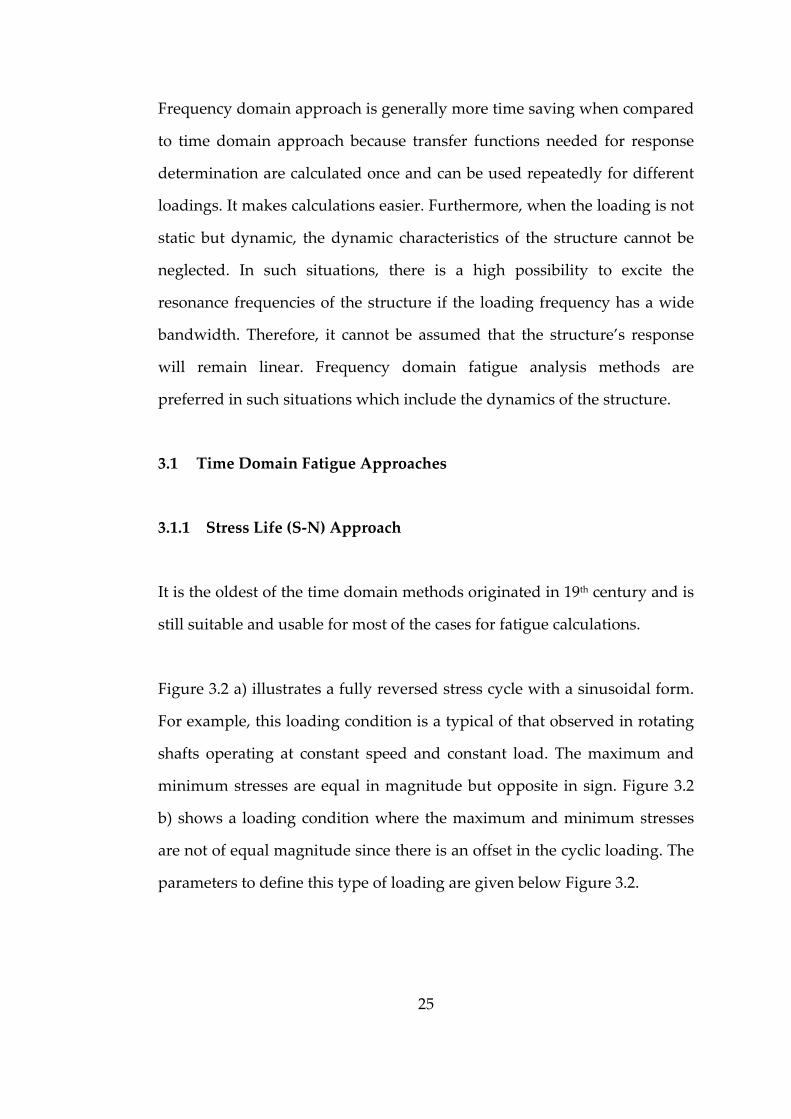
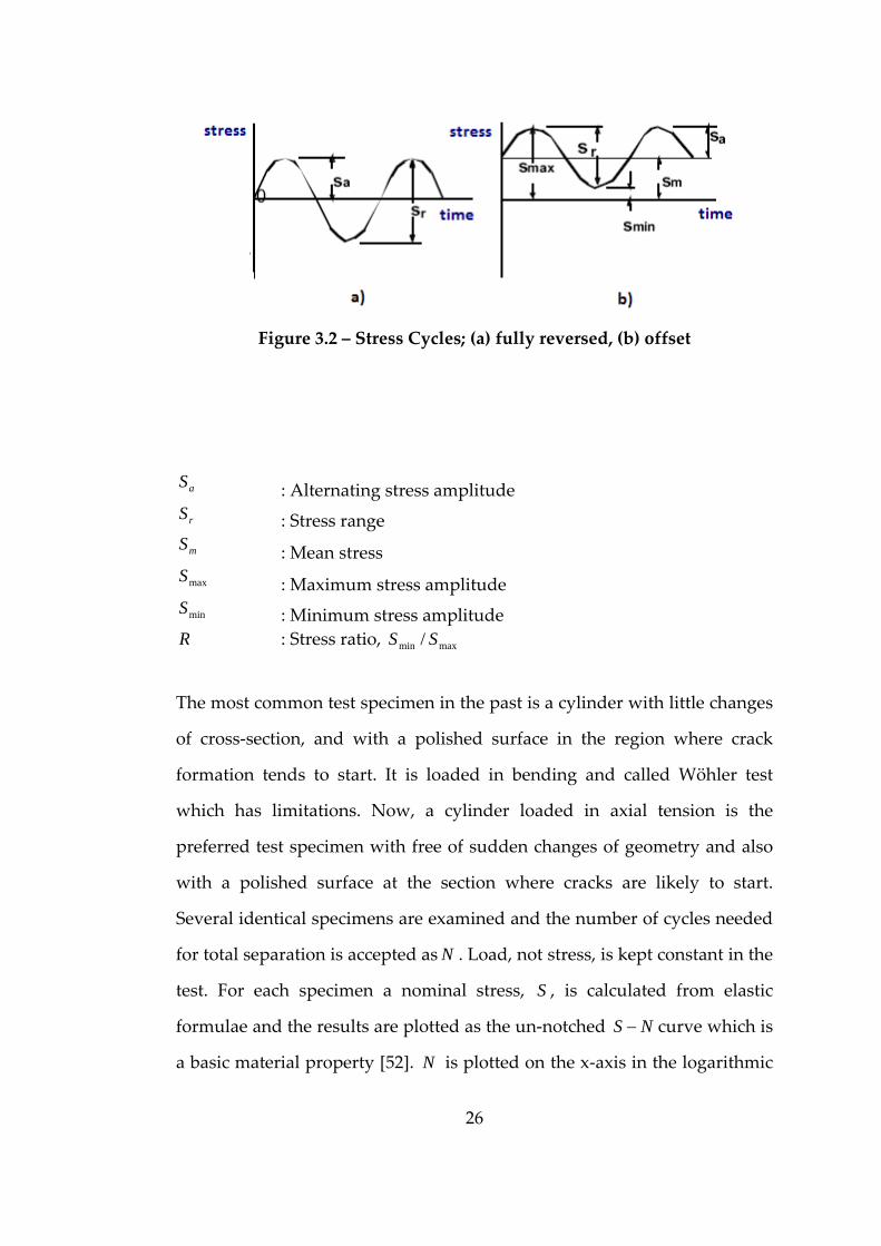
Figure 3.2 a) illustrates a fully reversed stress cycle with a sinusoidal form.
For example, this loading condition is a typical of that observed in rotating
shafts operating at constant speed and constant load. The maximum and
minimum stresses are equal in magnitude but opposite in sign. Figure 3.2
b) shows a loading condition where the maximum and minimum stresses
are not of equal magnitude since there is an offset in the cyclic loading. The
parameters to define this type of loading are given below Figure 3.2.
26
Figure 3.2 – Stress Cycles; (a) fully reversed, (b) offset
aS : Alternating stress amplitude rS : Stress range mS : Mean stress maxS : Maximum stress amplitude minS : Minimum stress amplitude
R : Stress ratio, maxmin / SS
The most common test specimen in the past is a cylinder with little changes
of cross‐section, and with a polished surface in the region where crack
formation tends to start. It is loaded in bending and called Wöhler test
which has limitations. Now, a cylinder loaded in axial tension is the
preferred test specimen with free of sudden changes of geometry and also
with a polished surface at the section where cracks are likely to start.
Several identical specimens are examined and the number of cycles needed
for total separation is accepted as N . Load, not stress, is kept constant in the
test. For each specimen a nominal stress, S , is calculated from elastic
formulae and the results are plotted as the un‐notched NS − curve which is
a basic material property [52]. N is plotted on the x‐axis in the logarithmic
27
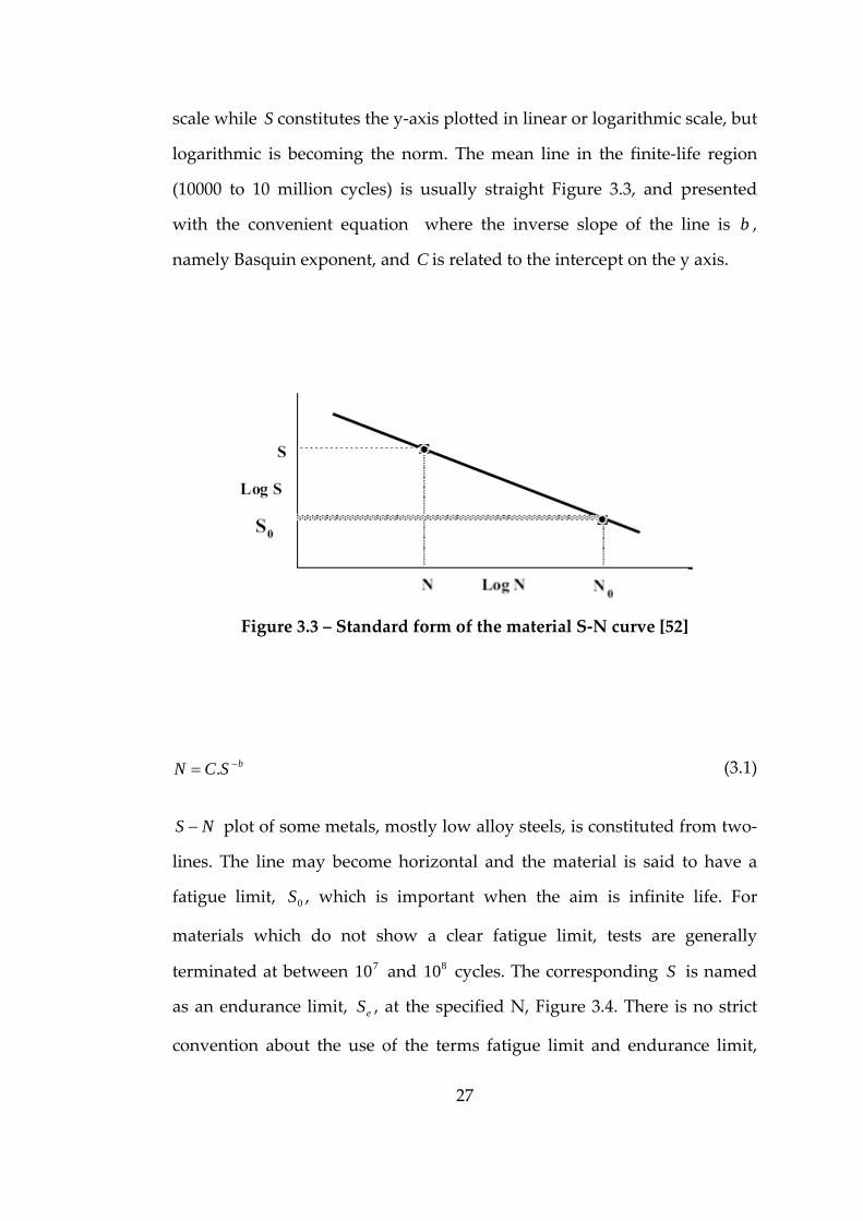
scale while S constitutes the y‐axis plotted in linear or logarithmic scale, but
logarithmic is becoming the norm. The mean line in the finite‐life region
(10000 to 10 million cycles) is usually straight Figure 3.3, and presented
with the convenient equation where the inverse slope of the line is b ,
namely Basquin exponent, and C is related to the intercept on the y axis.
Figure 3.3 – Standard form of the material S‐N curve [52]
(3.1)
NS − plot of some metals, mostly low alloy steels, is constituted from two‐
lines. The line may become horizontal and the material is said to have a
fatigue limit, 0S , which is important when the aim is infinite life. For
materials which do not show a clear fatigue limit, tests are generally
terminated at between 710 and 810 cycles. The corresponding S is named
as an endurance limit, eS , at the specified N, Figure 3.4. There is no strict
convention about the use of the terms fatigue limit and endurance limit,
bSCN −= .
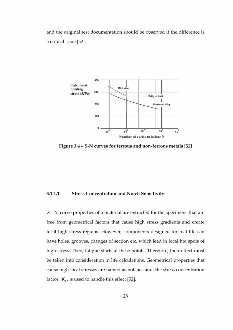
28
and the original test documentation should be observed if the difference is
a critical issue [52].
Figure 3.4 – S‐N curves for ferrous and non‐ferrous metals [52]
3.1.1.1 Stress Concentration and Notch Sensitivity
NS − curve properties of a material are extracted for the specimens that are
free from geometrical factors that cause high stress gradients and create
local high stress regions. However, components designed for real life can
have holes, grooves, changes of section etc. which lead in local hot spots of
high stress. Then, fatigue starts at these points. Therefore, their effect must
be taken into consideration in life calculations. Geometrical properties that
cause high local stresses are named as notches and, the stress concentration
factor, tK , is used to handle this effect [52].
29
(3.2)
fK is a reduced value of tK and generally called fatigue strength
concentration factor and described by (3.3) [1].
(3.3)
Then, notch sensitivity, q , is defined as (3.4) [1].
(3.4)
For simple loading, it is convenient to reduce the endurance limit by
dividing the unnotched specimen endurance limit by fK or multiplying
the reversing stress by fK [1].
3.1.1.2 Endurance Limit Modifying Factors
It is not realistic to expect the endurance limit of a structural part to match
the values obtained in the laboratory [1]. All effects of endurance limit
modifying factors are investigated in the equation given below (3.5).
(3.5)
where
ak : surface condition modification factor
notchthefromremote stress Nominalnotch theofregion in the stress Maximum
=tK
11
−
−=
t
f
KK
q
specimen freenotch in Stressspecimen notchedin stress Maximum
=fK
'efedcbae SkkkkkkS =
30
bk : size modification factor
ck : load modification factor
dk : temperature modification factor
ek : reliability factor
fk : miscellaneous‐effects modification factor
'eS : laboratory test specimen endurance limit
eS : endurance limit at the critical location of a machine part in the
geometry and condition of use.
3.1.1.3 Mean Stress Effect
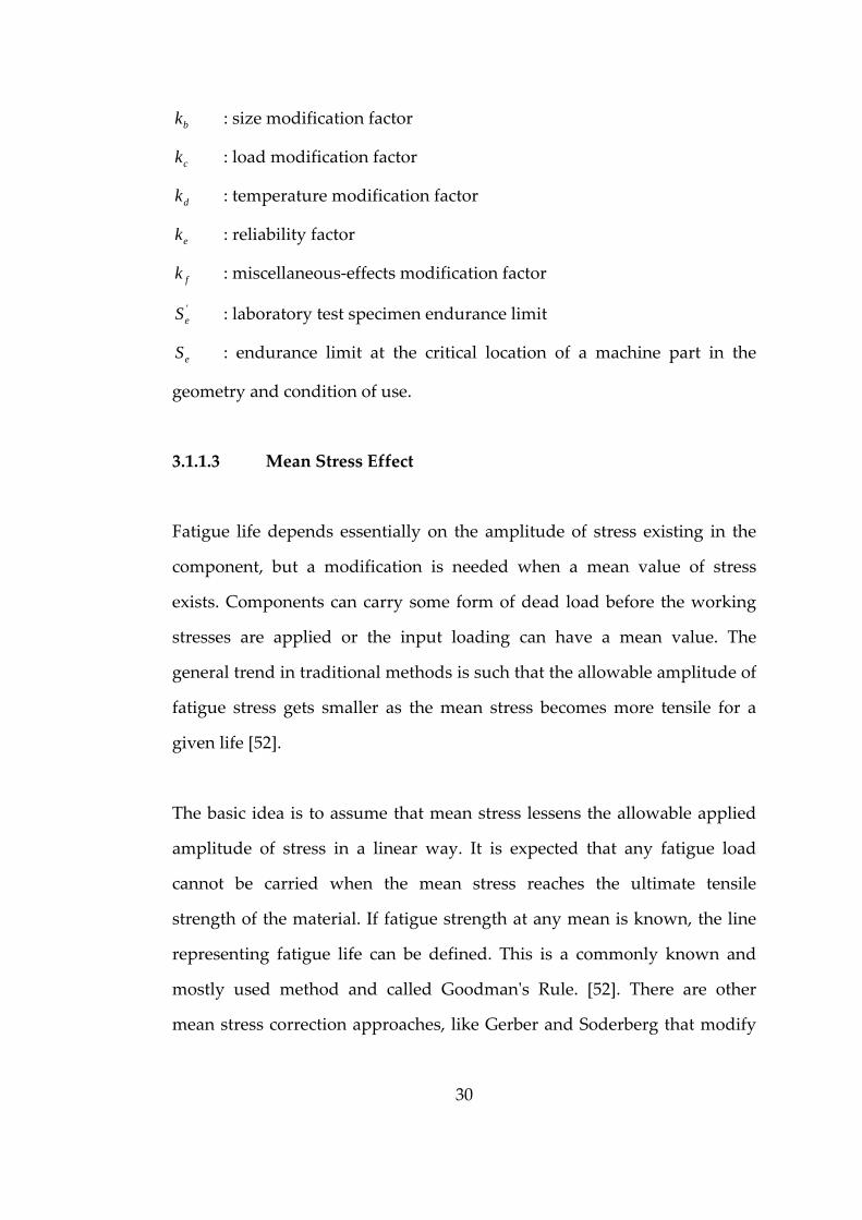
Fatigue life depends essentially on the amplitude of stress existing in the
component, but a modification is needed when a mean value of stress
exists. Components can carry some form of dead load before the working
stresses are applied or the input loading can have a mean value. The
general trend in traditional methods is such that the allowable amplitude of
fatigue stress gets smaller as the mean stress becomes more tensile for a
given life [52].
The basic idea is to assume that mean stress lessens the allowable applied
amplitude of stress in a linear way. It is expected that any fatigue load
cannot be carried when the mean stress reaches the ultimate tensile
strength of the material. If fatigue strength at any mean is known, the line
representing fatigue life can be defined. This is a commonly known and
mostly used method and called Goodmanʹs Rule. [52]. There are other
mean stress correction approaches, like Gerber and Soderberg that modify
31
alternating stress according to mean stress. Mean stress correction methods’
graphical representations are illustrated in Figure 3.5.
Figure 3.5 ‐ Mean Stress Modification Methods [1]
Goodman’s Model:
(3.6)
Gerber’s Model:
(3.7)
1' =+u
m
a
a
SS
SS
12
' =⎟⎟⎠
⎞⎜⎜⎝
⎛+
u
m
a
a
SS
SS
32
Soderberg’s Model:
(3.8)
aS : Alternating stress
'aS : Equivalent alternating stress
mS : Mean stress
uS : Ultimate tensile strength
yS : Tensile yield strength
3.1.1.4 Variable Amplitude Loading and Fatigue Damage
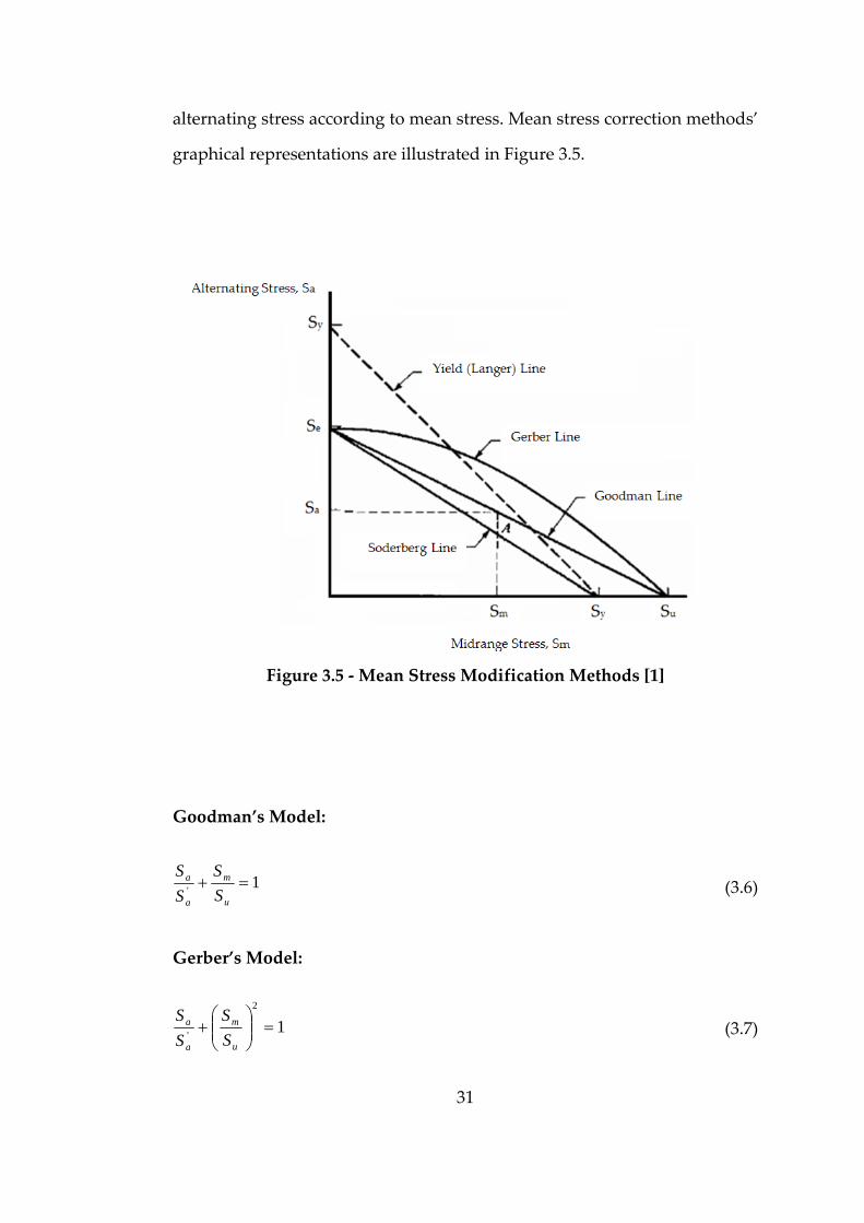
The investigation of metal fatigue under variable amplitude loading is
based on the study of cumulative damage. The variable amplitude time
history consists of 1n cycles of amplitude 1S , 2n of amplitude 2S , 3n of
amplitude 3S and so on. Usually the pattern repeats itself after a small
number of stress cycles, nS (Figure 3.6). The sequence up to nS is then
called block, and the aim is to determine the number of the blocks that can
be applied until failure occurs. The method commonly used is known as
Miner or Palmgren‐Miner rule. According to Miner’s hypothesis, linear
damage accumulation is assumed. First, when the 1S level of stress that
repeats 1n cycles is considered, the number of life cycles at stress level 1S
that would cause fatigue failure if no other stresses were present can be
obtained from NS − curve . Calling this number of cycles as 1N , it is
assumed that 1n cycles of 1S use up a fraction 11 / Nn of the total fatigue life.
1' =+y
m
a
a
SS
SS
33
This shows the damage fraction that 1n cycles cause. The total damage
fraction for one block is obtained by doing a similar calculation for all other
stresses and summing all the damage fraction results [52]. Then, expected
damage, [ ]DE , is equated to this summation and set to one to calculate
fatigue life (3.9). The order of stresses occurring in history is ignored in
Miner’s rule.
Figure 3.6 – Block Loading Sequence
(3.9)
3.1.1.5 Counting Methods
Most of the engineering components in real life are exposed to stress
responses that are more complex than shown in Figure 3.6. When
individual stress cycles causing fatigue damage cannot be distinguished
[ ] 1...1 2
2
1
1 =+++== ∑= n
nn
i i
i
Nn
Nn
Nn
Nn
DE
34
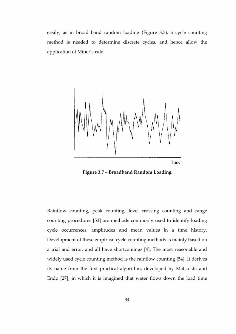
easily, as in broad band random loading (Figure 3.7), a cycle counting
method is needed to determine discrete cycles, and hence allow the
application of Miner’s rule.
Figure 3.7 – Broadband Random Loading
Rainflow counting, peak counting, level crossing counting and range
counting procedures [53] are methods commonly used to identify loading
cycle occurrences, amplitudes and mean values in a time history.
Development of these empirical cycle counting methods is mainly based on
a trial and error, and all have shortcomings [4]. The most reasonable and
widely used cycle counting method is the rainflow counting [54]. It derives
its name from the first practical algorithm, developed by Matsuishi and
Endo [27], in which it is imagined that water flows down the load time

35
history, with the axes reversed. An algorithm is developed for counting
Rainflow cycles. The most common procedure is as follows [52]:
Peaks and troughs from the time signal are extracted so that all points
between adjacent peaks and troughs are discarded.
The beginning and end of the sequence are arranged to have the same
level. The simplest way is to add an additional point at the end of the
signal to match the beginning.
The highest peak is found and the signal is reordered so that this
becomes the beginning and the end. The beginning and end of the
original signal have to be joined together.
Procedure is started at the beginning of the sequence and consecutive
sets of four peaks and troughs are picked. A rule is applied that states,
If the second segment is shorter (vertically) than the first, and the third is
longer than the second, the middle segment can be extracted and recorded
as a Rainflow cycle. In this case, B and C are completely enclosed by A and
D (Figure 3.8).
Figure 3.8 – Rainflow Cycles [52]
36
If no cycle is counted then a check is made on the next set of four peaks,
i.e. peaks 2 to 5, and so on until a Rainflow cycle is counted. Every time
a Rainflow cycle is counted the procedure is started from the beginning
of the sequence again.
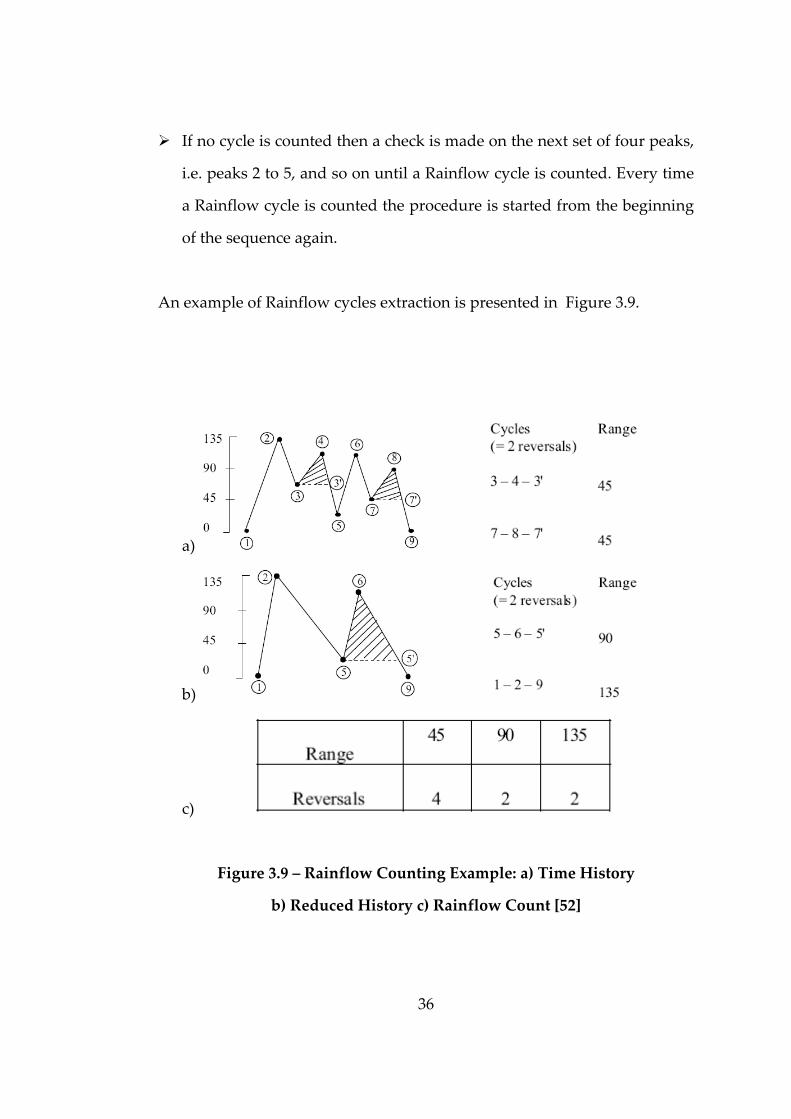
An example of Rainflow cycles extraction is presented in Figure 3.9.
a)
b)
c)
Figure 3.9 – Rainflow Counting Example: a) Time History
b) Reduced History c) Rainflow Count [52]
37
3.1.2 Strain Life Approach
When loading cycles are severe, another type of fatigue behavior emerges.
In this regime, the cyclic loads are relatively large and lead in significant
amounts of plastic deformation resulting in relatively short lives.
In this approach, Strain‐Cycle curve should be used rather than Stress‐
Cycle curve ( NS − ) to obtain fatigue life. Strain‐Cycle curve can be
obtained by cyclic tests where the strain is held constant via closed loop
control test equipment.
3.1.3 Crack Propagation Approach
When an initial crack exists in the structure, then crack propagation is
followed. The crack growth analytical calculation is done by means of
Linear Elastic Fracture Mechanics theory.
3.2 Frequency Domain Approach
When the loading is not static but dynamic, the dynamics of the structure
should be taken into account. There is high possibility to excite the
resonance frequencies of the structure if the loading frequency has a wide
bandwidth. When this situation occurs, it cannot be assumed that the
structure’s response to the loading will remain linear in the frequency
domain. Therefore, to overcome such situations, frequency domain fatigue
analysis methods are applied which do not neglect the vibrant properties of
the structure.

38
A general way of representing the random data in the frequency domain is
using Power Spectral Density (PSD) which is an alternative way of
specifying the time signal. The PSD illustrates the frequency content of the
time signal. It is obtained by utilizing Fourier Transformation.
A periodic time history, )(ty , can be represented by the summation of a
series of sine and cosine waves of different amplitude, frequency and phase
which is the basis of Fourier series expansion expressed by (3.10) [55].
(3.10)
where pT denotes for period and
(3.11)
(3.12)
(3.13)
0A , nA and nB are Fourier coefficients which yield information about the
frequency content of the time history. 0A denotes the mean value of the
time history as nA and nB show the amplitudes of the various sines and
cosines which constitute time history when added together.
∑∞
= ⎪⎭
⎪⎬⎫
⎪⎩
⎪⎨⎧
⎟⎟⎠
⎞⎜⎜⎝
⎛+⎟
⎟⎠
⎞⎜⎜⎝
⎛+=
10
2sin2cos)(n p
np
n tT
nBtT
nAAty ππ
∫−
=2
2
0 )(1p
p
T
Tp
dttyT
A
∫−
⎟⎟⎠
⎞⎜⎜⎝
⎛=
2
2
2cos)(2p
p
T
T ppn dtt
Tnty
TA π
∫−
⎟⎟⎠
⎞⎜⎜⎝
⎛=
2
2
2sin)(2p
p
T
T ppn dtt
Tnty
TB π
39
To express the time series with its frequency content, a transformation
between the time and frequency domain is achieved by means of Fourier
transformation. In this sense, )( fy entails a description of the time history
)(ty in the frequency domain ʹ f ʹ. The Fourier transform pair given in (3.14)
and (3.15) enables transformations between the two domains effectively.
(3.14)
(3.15)
As well as the integral form, the Fourier transformation can also be
depicted in a discrete form. This usage is mostly favorable because time
histories are generally measured in a discrete, digitized form with equally
spaced intervals in time. In these conditions, the integral form is difficult to
process. Therefore, some numerical calculations are carried out on the
measured time history to transform it into the frequency domain which is
called Discrete Fourier Transform. The result obtained from a discrete
transformation is liable to approximate the result obtained from an integral
transformation as the sample length and sampling frequency increase [11].
Cooley and Tukey [56] develops a very rapid discrete Fourier transform
algorithm called Fast Fourier Transform (FFT) and has a reverse process
named the Inverse Fourier Transform (IFFT). The discrete form of Fourier
transformation is given by
(3.16)
(3.17)
∫∞
∞−
−= dtetyfy tfi )2()()( π
∫∞
∞−
= dfefyty tfi )2()()( π
kN
ni
kk
pn ety
NT
fy⎟⎠⎞
⎜⎝⎛
∑=π2
)()(
nN
ki
nn
pk efy
Tty
⎟⎠⎞
⎜⎝⎛
∑=π2
)(1)(
40
where pT is the period of the function )( kty and N is the number of data
points for Fourier transform.
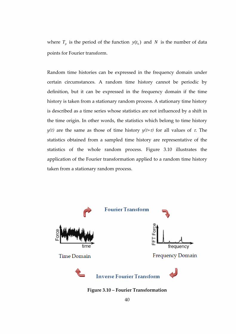
Random time histories can be expressed in the frequency domain under
certain circumstances. A random time history cannot be periodic by
definition, but it can be expressed in the frequency domain if the time
history is taken from a stationary random process. A stationary time history
is described as a time series whose statistics are not influenced by a shift in
the time origin. In other words, the statistics which belong to time history
y(t) are the same as those of time history y(t+τ) for all values of τ. The
statistics obtained from a sampled time history are representative of the
statistics of the whole random process. Figure 3.10 illustrates the
application of the Fourier transformation applied to a random time history
taken from a stationary random process.
Figure 3.10 – Fourier Transformation
41
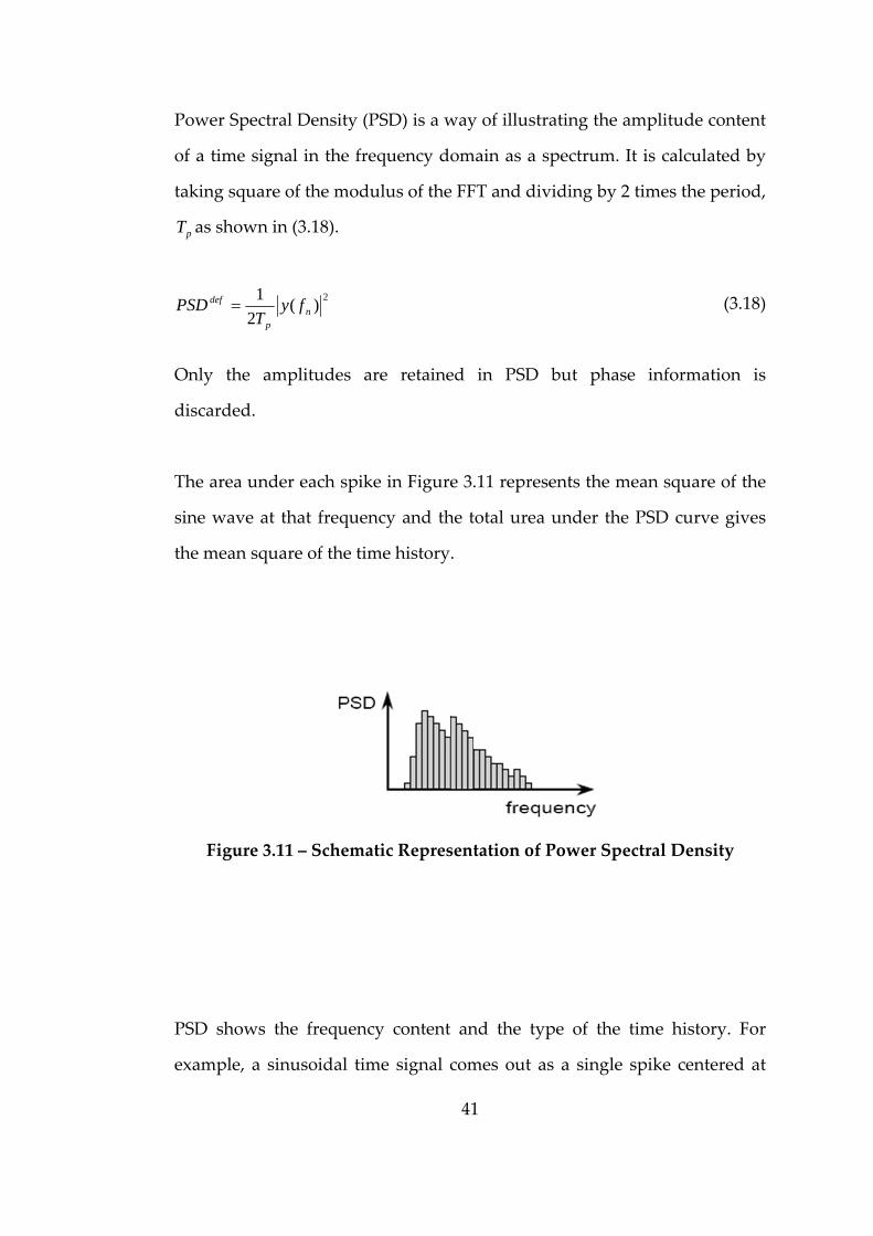
Power Spectral Density (PSD) is a way of illustrating the amplitude content
of a time signal in the frequency domain as a spectrum. It is calculated by
taking square of the modulus of the FFT and dividing by 2 times the period,
pT as shown in (3.18).
(3.18)
Only the amplitudes are retained in PSD but phase information is
discarded.
The area under each spike in Figure 3.11 represents the mean square of the
sine wave at that frequency and the total urea under the PSD curve gives
the mean square of the time history.
Figure 3.11 – Schematic Representation of Power Spectral Density
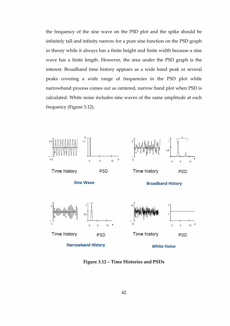
PSD shows the frequency content and the type of the time history. For
example, a sinusoidal time signal comes out as a single spike centered at
2)(2
1n
p
def fyT
PSD =
42
the frequency of the sine wave on the PSD plot and the spike should be
infinitely tall and infinity narrow for a pure sine function on the PSD graph
in theory while it always has a finite height and finite width because a sine
wave has a finite length. However, the area under the PSD graph is the
interest. Broadband time history appears as a wide band peak or several
peaks covering a wide range of frequencies in the PSD plot while
narrowband process comes out as centered, narrow band plot when PSD is
calculated. White noise includes sine waves of the same amplitude at each
frequency (Figure 3.12).
Figure 3.12 – Time Histories and PSDs
43
In linear systems, the output is related to the input by a linear transfer
function. The response of a linear system to a single random process is
obtained by means of transfer functions obtained via frequency response
analysis of the structure where for each frequency a different transfer
function is calculated:
(3.19)
where )( fFFTr and )( fFFTi stands for FFT of the response, stress in this
thesis, and FFT of the input loading, acceleration in this thesis, respectively.
)( fH represents the transfer function of the system in frequency domain. It
is convenient to obtain the response, stress, as a PSD, )( fGr (3.20). If the
input, acceleration, is also expressed as PSD, )( fGi , then the PSD of output
is given by means of a linear transfer function, )( fH , its conjugate, )(* fH
and input PSD in the frequency domain where )(* fFFTi is complex
conjugate of the input FFT (3.21).
(3.20)
(3.21)
Then, (3.21) can be rewritten in the form of (3.22), where )( fGr is equal to
input PSD times modulus squared of transfer function.
(3.22)
)()()( fFFTfHfFFT ir ×=
( ))()()()(2
1)( ** fFFTfHfFFTfHT
fG iip
r ×××⎟⎟⎠
⎞⎜⎜⎝
⎛=
)()()()( * fGfHfHfG ir ××=
)()()( 2 fGfHfG ir ×=
44
Stress PSD is directly used for vibration fatigue life calculations which will
be explained in the proceeding parts of this thesis in detail.
In vibration fatigue calculations, the frequency content of the stresses is
accounted for by a probability density function (PDF) of rainflow stress
ranges, )(Sp . The most convenient way, mathematically, of storing stress
range histogram information is in the form of a probability density function
of stress ranges Figure 3.13. The bin width, dS , and the total number of
cycles recorded in the histogram, tS , are required to transform from a stress
range histogram to a PDF, or back.
Figure 3.13 – Probability Density Function
The probability of the stress range occurring between 2
dSSi − and 2
dSSi +
is calculated as the multiplication of ( )iSp and dS while to get PDF from
45
rainflow histogram, each bin height is divided by dSSt . Then, number of
cycles at the particular stress level S , )(Sn is stated as in (3.23).
(3.23)
The total number of cycles at the stress level S that causes failure according
to Woehler curve, )(SN , is expressed as in (3.24) where C and b stand for
material constant and Basquin exponent respectively.
(3.24)
Then, fatigue life calculation is performed by utilizing (3.25) that equates
(3.26) in turn where total number of cycles in required time, tS , is equal to
[ ]TPE . T is the fatigue life in seconds and [ ]DE is expected value of
damage. Fatigue life is found setting [ ]DE to unity. The order of stresses
occurring in history is ignored in Miner’s rule. However, this does not
create a problem for vibration fatigue solution since the loading’s statistical
properties are important and the loading is random, stationary and
Gaussian.
(3.25)
(3.26)
( )dSStSpSni =)(
bi SCSN =)(
[ ] [ ] ( )∫∑∞
==0)(
)(dSSpS
CTPE
SNSn
DE b
i i
i
[ ] ( )∫∑∞
==0)(
)(dSSpS
CS
SNSn
DE bt
i i
i
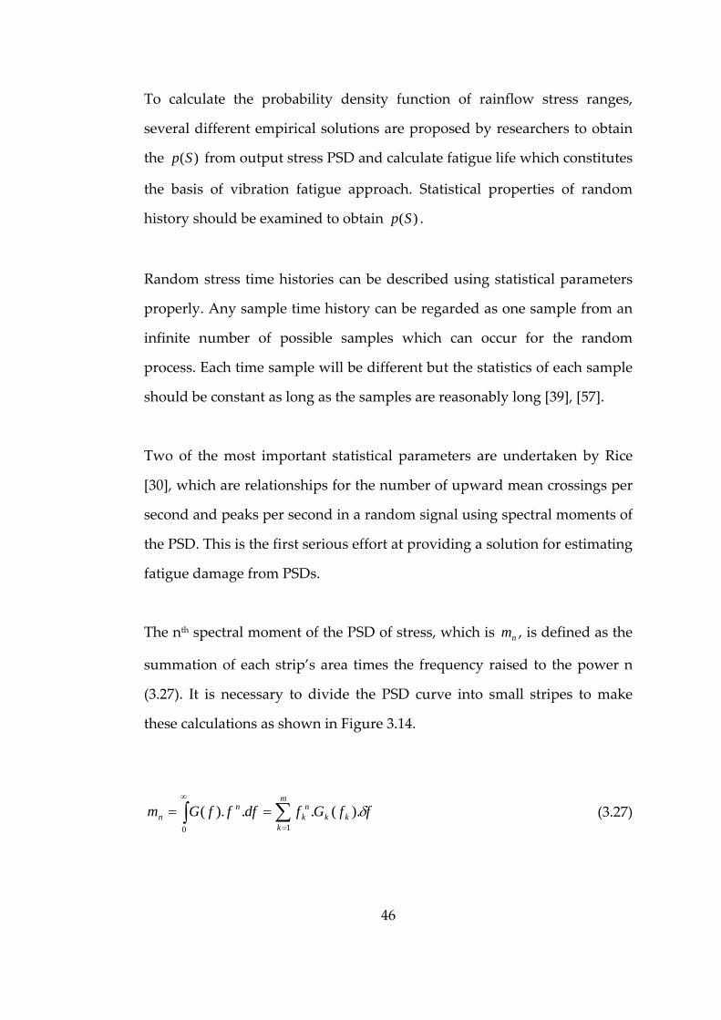
46
To calculate the probability density function of rainflow stress ranges,
several different empirical solutions are proposed by researchers to obtain
the )(Sp from output stress PSD and calculate fatigue life which constitutes
the basis of vibration fatigue approach. Statistical properties of random
history should be examined to obtain )(Sp .
Random stress time histories can be described using statistical parameters
properly. Any sample time history can be regarded as one sample from an
infinite number of possible samples which can occur for the random
process. Each time sample will be different but the statistics of each sample
should be constant as long as the samples are reasonably long [39], [57].
Two of the most important statistical parameters are undertaken by Rice
[30], which are relationships for the number of upward mean crossings per
second and peaks per second in a random signal using spectral moments of
the PSD. This is the first serious effort at providing a solution for estimating
fatigue damage from PSDs.
The nth spectral moment of the PSD of stress, which is nm , is defined as the
summation of each strip’s area times the frequency raised to the power n
(3.27). It is necessary to divide the PSD curve into small stripes to make
these calculations as shown in Figure 3.14.
(3.27)
∫ ∑∞
=
==0 1
).(..).(m
kkk
nk
nn ffGfdfffGm δ
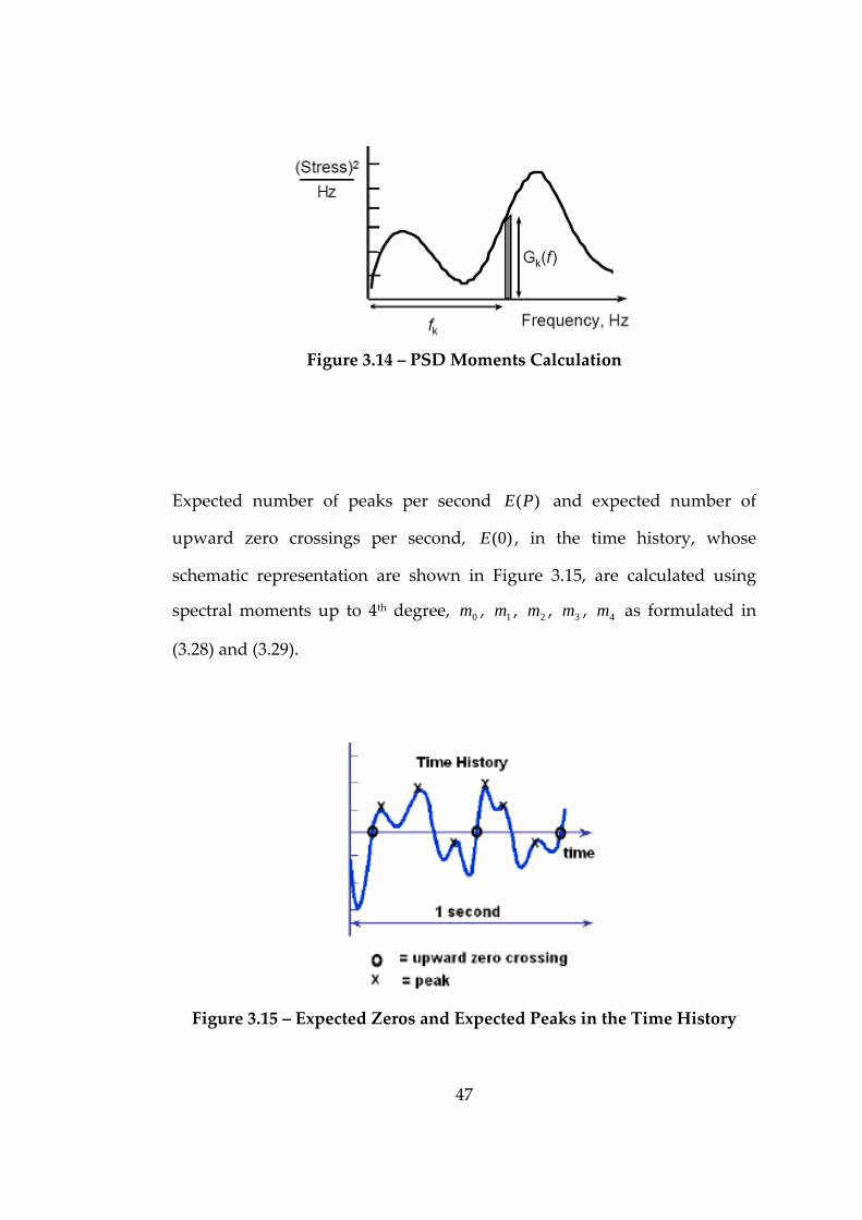
47
Figure 3.14 – PSD Moments Calculation
Expected number of peaks per second )(PE and expected number of
upward zero crossings per second, )0(E , in the time history, whose
schematic representation are shown in Figure 3.15, are calculated using
spectral moments up to 4th degree, 0m , 1m , 2m , 3m , 4m as formulated in
(3.28) and (3.29).
Figure 3.15 – Expected Zeros and Expected Peaks in the Time History
48
(3.28)
(3.29)
Another important statistical parameter is irregularity factor, γ , which is
the ratio of expected number of zeros per second over expected number of
peaks per second. It is a measure of frequency band the history cover on
PSD graph in the sense that as the irregularity factor approaches to one, the
process gets closer to narrow band process, and as the irregularity factor
approaches to zero, the process gets closer to broadband process. In other
words, a value of one corresponds to a narrow band signal which means
that the signal contains only one predominant frequency while a value of
zero implies that the signal contains an equal amount of energy at all
frequencies.
(3.30)
All these statistical information gathered from the stress PSD is used for
vibration fatigue calculations.
3.2.1 Narrow Band Approach
The first frequency domain method on calculating fatigue damage from
PSDʹs is called narrow band approach. Bendat [31] assumes that all positive
peaks in the time history is followed by corresponding troughs of similar
magnitude regardless of whether they actually formed stress cycles, in
0
2
2
4
]0[
][
mm
E
mmPE
=
=
40
22
][]0[
mmm
PEE
==γ
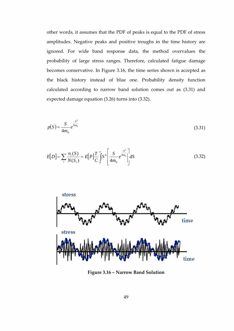
49
other words, it assumes that the PDF of peaks is equal to the PDF of stress
amplitudes. Negative peaks and positive troughs in the time history are
ignored. For wide band response data, the method overvalues the
probability of large stress ranges. Therefore, calculated fatigue damage
becomes conservative. In Figure 3.16, the time series shown is accepted as
the black history instead of blue one. Probability density function
calculated according to narrow band solution comes out as (3.31) and
expected damage equation (3.26) turns into (3.32).
(3.31)
(3.32)
Figure 3.16 – Narrow Band Solution
( ) 0
2
8
04mS
emSSp
−
=
[ ] [ ] ∫∑∞ −
⎥⎥⎦
⎤
⎢⎢⎣
⎡==
0
8
0
0
2
4)()(
dSemSS
CTPE
SNSn
DE mS
b
i i
i
50
3.2.2 Empirical Correction Factors
Many expressions are proposed to correct the conservatism of narrow band
solution. Generally, they are constituted by generating sample time
histories from PSDʹs by means of inverse Fourier transformation. A
conventional rainflow cycle count is obtained from these data sets.
The solutions of Wirsching et al [32], Chaudhury and Dover [33], Tunna
[34] and Hancock [35] are all developed making use of this approach and
are all expressed in terms of the spectral moments up to the forth degree.
Wirschingʹs Equation:
(3.33)
where
(3.34)
(3.35)
(3.36)
Hancockʹs Equation:
(3.37)
This solution is proposed in the form of an equivalent stress range
parameter, hS , where
(3.38)
[ ] [ ] ( ) ( )( )( )( ))(11 bcNB babaDEDE ε−−+=
( ) bba 033.0926.0 −=
( ) 323.2587.1 −= bbc21 γε −=
⎥⎦
⎤⎢⎣
⎡⎟⎠⎞
⎜⎝⎛ +Γ⎟
⎠⎞⎜
⎝⎛= 1
222 0
bmSbbb
h γ
( )∫= dSSpSS bbh
51
Chaudhury and Dover Equation:
(3.39)
Tunna Equation:
(3.40)
3.2.3 Steinberg’s Solution
Steinberg [36] proposes a three‐band technique as a rough estimation for
the fatigue damage calculation. This method is based on the Gaussian
distribution. The instantaneous stress values in the time history are
assumed for the 3 bands where σ stands for standard deviation:
• 1σ values occur 68.3% of the time
• 2σ values occur 27.1% of the time
• 3σ values occur 4.33% of the time
Therefore, the fatigue damage is estimated based on these three stress
levels. This approach is a very simple solution based on the assumption
that no stress cycles occur with ranges greater than 6 rms values. The
distribution of stress ranges is then specified to follow a Gaussian
distribution. This method is preferred in the electronics industry, as a tool
for comparison.
[ ] [ ] bhS
CTPEDE =
( ) 0
2
8
04me
mSSp γ
δ
γ
−
=
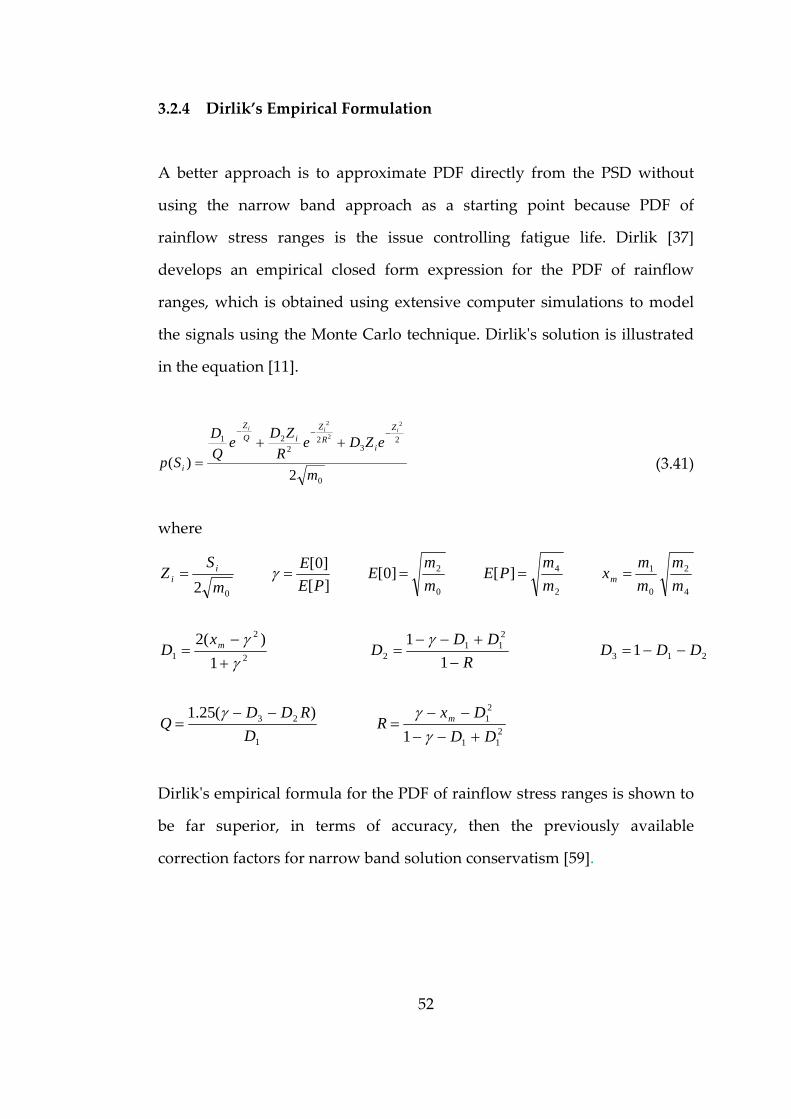
52
3.2.4 Dirlik’s Empirical Formulation
A better approach is to approximate PDF directly from the PSD without
using the narrow band approach as a starting point because PDF of
rainflow stress ranges is the issue controlling fatigue life. Dirlik [37]
develops an empirical closed form expression for the PDF of rainflow
ranges, which is obtained using extensive computer simulations to model
the signals using the Monte Carlo technique. Dirlikʹs solution is illustrated
in the equation [11].
(3.41)
where
211
21
1
23
213
211
22
2
1
4
2
0
1
2
4
0
2
0
1)(25.1
11
11
)(2
][]0[][]0[
2
DDDx
RD
RDDQ
DDDR
DDD
xD
mm
mm
xmm
PEmm
EPE
Em
SZ
m
m
mi
i
+−−−−
=−−
=
−−=−
+−−=
+−
=
=====
γγγ
γγγ
γ
Dirlikʹs empirical formula for the PDF of rainflow stress ranges is shown to
be far superior, in terms of accuracy, then the previously available
correction factors for narrow band solution conservatism [59].
0
23
22
21
2)(
2
2
2
m
eZDeR
ZDeQD
Sp
iii Z
iR
ZiQ
Z
i
−−−
++=
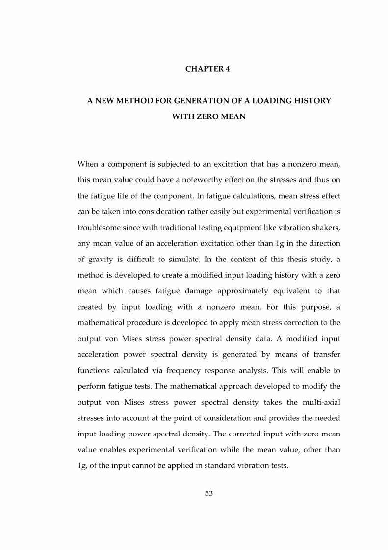
53
CHAPTER 4
A NEW METHOD FOR GENERATION OF A LOADING HISTORY
WITH ZERO MEAN
When a component is subjected to an excitation that has a nonzero mean,
this mean value could have a noteworthy effect on the stresses and thus on
the fatigue life of the component. In fatigue calculations, mean stress effect
can be taken into consideration rather easily but experimental verification is
troublesome since with traditional testing equipment like vibration shakers,
any mean value of an acceleration excitation other than 1g in the direction
of gravity is difficult to simulate. In the content of this thesis study, a
method is developed to create a modified input loading history with a zero
mean which causes fatigue damage approximately equivalent to that
created by input loading with a nonzero mean. For this purpose, a
mathematical procedure is developed to apply mean stress correction to the
output von Mises stress power spectral density data. A modified input
acceleration power spectral density is generated by means of transfer
functions calculated via frequency response analysis. This will enable to
perform fatigue tests. The mathematical approach developed to modify the
output von Mises stress power spectral density takes the multi‐axial
stresses into account at the point of consideration and provides the needed
input loading power spectral density. The corrected input with zero mean
value enables experimental verification while the mean value, other than
1g, of the input cannot be applied in standard vibration tests.
54
Time domain fatigue life calculation techniques directly utilize mean stress
correction methods to amplify the stress ranges to take the mean stress
effect into account. In frequency domain fatigue life calculation approaches,
when the power spectral density of the stress is determined, only the
variable stress part is considered, however, the constant mean component
is ignored [60]. In this study, the mean stress correction is accomplished on
von Mises stress power spectral density to be able to include the loading’s
bias effect. Goodman correction technique is preferred to Gerber since it is
reported in [61] that Gerber relationship generally gives higher fatigue lives
compared to the experimental results. Dirlik method is chosen for
application of vibration fatigue approach. According to [59], Dirlik
approach leads to better results in comparison to the corresponding time
domain and frequency response methods.
An aluminum (2024 T4) plate fixed and excited at one end is used for the
implementation which is shown schematically in Figure 4.1, whose
dimensions are given in Table 4.1. The base excitation leads to a fully three
dimensional multi‐axial state of stress in the plate.
It is shown that the developed method is useful in creating a modified
input acceleration data with a zero mean that can simulate damage for a
selected point in the structure under consideration. Equivalent input
loading obtained by means of the aforementioned method is convenient
and conservative for experimental applications. Besides being a time saving
method, it is suitable to be implemented for any type of loading.
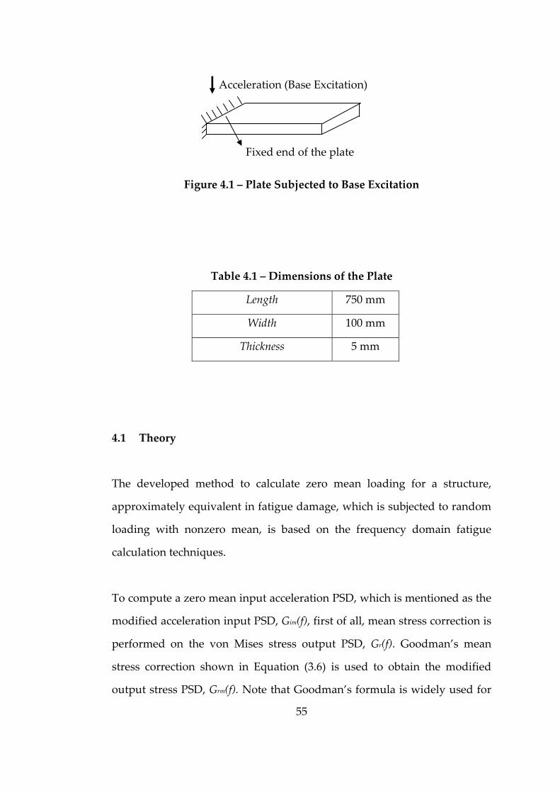
55
Figure 4.1 – Plate Subjected to Base Excitation
Table 4.1 – Dimensions of the Plate
Length 750 mm
Width 100 mm
Thickness 5 mm
4.1 Theory
The developed method to calculate zero mean loading for a structure,
approximately equivalent in fatigue damage, which is subjected to random
loading with nonzero mean, is based on the frequency domain fatigue
calculation techniques.
To compute a zero mean input acceleration PSD, which is mentioned as the
modified acceleration input PSD, Gim(f), first of all, mean stress correction is
performed on the von Mises stress output PSD, Gr(f). Goodman’s mean
stress correction shown in Equation (3.6) is used to obtain the modified
output stress PSD, Grm(f). Note that Goodman’s formula is widely used for
Fixed end of the plate
Acceleration (Base Excitation)
56
mean stress correction for stress amplitude modification [62], but in this
study it is utilized to correct PSD of von Mises stress output data. If the PSD
is split into equal strips, the area of each strip can be utilized to obtain an
equivalent sine wave. The amplitude of each equivalent sine wave is equal
to the square root of the area times 2 . This is because of the fact that the
root mean square of a sine wave is equal to its amplitude divided by 2 ,
and the root mean square of each strip in the PSD is equal to the square root
of its area [39]. In this study, the stress PSD value, Gr(f), is multiplied by the
corresponding frequency resolution and the square root of it is taken and
multiplied with 2 to obtain the alternating stress amplitude, Sa, for each
frequency. Then, mean stress correction is performed with (3.6) to calculate
the modified alternating stress amplitude, Sa’. Afterwards, the calculations
are carried out in the reverse direction to reach modified output stress PSD,
Grm(f).
Theoretically, there should be an input acceleration PSD that results in the
modified output stress PSD, Grm(f), when applied to the structure since the
transfer function of the structure remains the same regardless of input type.
This physical relation can be represented by the following equation which
is rewritten from (3.21) for a different input‐output couple.
(4.1)
According to (3.21);
(4.2)
)()()()( * fGfHfHfG imrm ××=
1* )()()()( −=× fxGfGfHfH ir
57
and from (4.1);
(4.3)
To obtain Gim(f), (4.2) and (4.3) are equated to each other and re‐ordered
which results in:
(4.4)
The variables in equation (4.4) are vectors, which in turn makes regular
matrix inversion impossible. Therefore, the inverse calculations in equation
(4.4) are carried out by using pseudo‐inverse. A corrected input loading
with zero mean but modified alternating stress, which creates fatigue
damage approximately equivalent to the damage caused by the
unprocessed loading with nonzero mean, is extracted by means of this
technique. It should be noted that, this approach is focusing to find a
modified loading that simulates damage for a selected point on the
structure, which in turn will be acceptable in the vicinity of that point only.
4.2 Case Study
The proposed correction method is demonstrated on an application
analyzed according to the method presented in Section 4.1.
The plate shown in Figure 4.1 is excited from its cantilevered base with
stationary, Gaussian, random, 10 second acceleration time history with a
non‐zero mean value of 3 g, as shown in Figure 4.2. Power spectral density
1* )()()()( −=× fxGfGfHfH imrm
[ ] 111 )()()()( −−−= fxGfxGfGfG irrmim
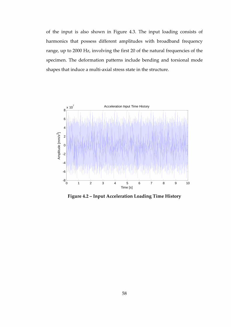
58
of the input is also shown in Figure 4.3. The input loading consists of
harmonics that possess different amplitudes with broadband frequency
range, up to 2000 Hz, involving the first 20 of the natural frequencies of the
specimen. The deformation patterns include bending and torsional mode
shapes that induce a multi‐axial stress state in the structure.
0 1 2 3 4 5 6 7 8 9 10-8
-6
-4
-2
0
2
4
6
8x 10⁷ Acceleration Input Time History
Time [s]
Am
plitu
de [m
m/s
2 ]
Figure 4.2 – Input Acceleration Loading Time History
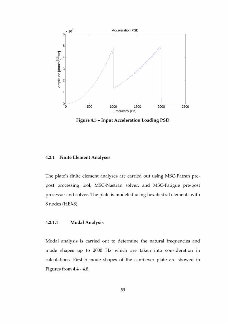
59
0 500 1000 1500 2000 25000
1
2
3
4
5
6x 10¹¹ Acceleration PSD
Frequency [Hz]
Am
plitu
de [(
mm
/s2 )2 /H
z]
Figure 4.3 – Input Acceleration Loading PSD
4.2.1 Finite Element Analyses
The plate’s finite element analyses are carried out using MSC‐Patran pre‐
post processing tool, MSC‐Nastran solver, and MSC‐Fatigue pre‐post
processor and solver. The plate is modeled using hexahedral elements with
8 nodes (HEX8).
4.2.1.1 Modal Analysis
Modal analysis is carried out to determine the natural frequencies and
mode shapes up to 2000 Hz which are taken into consideration in
calculations. First 5 mode shapes of the cantilever plate are showed in
Figures from 4.4 ‐ 4.8.
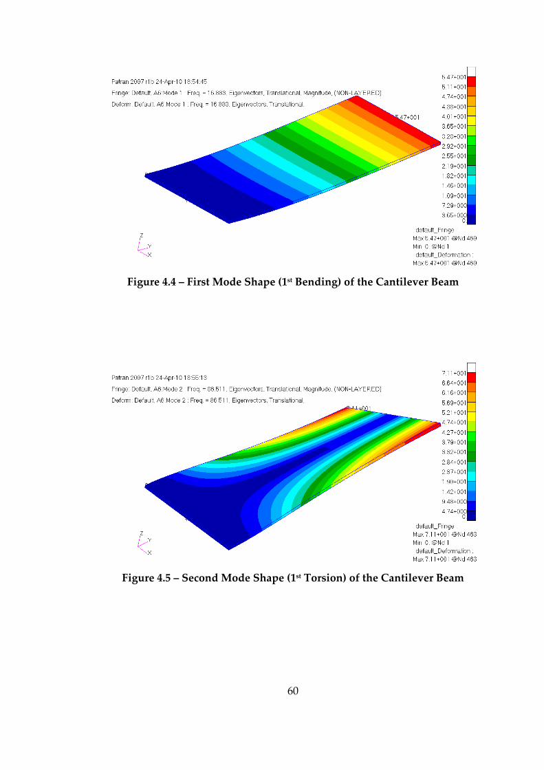
60
Figure 4.4 – First Mode Shape (1st Bending) of the Cantilever Beam
Figure 4.5 – Second Mode Shape (1st Torsion) of the Cantilever Beam
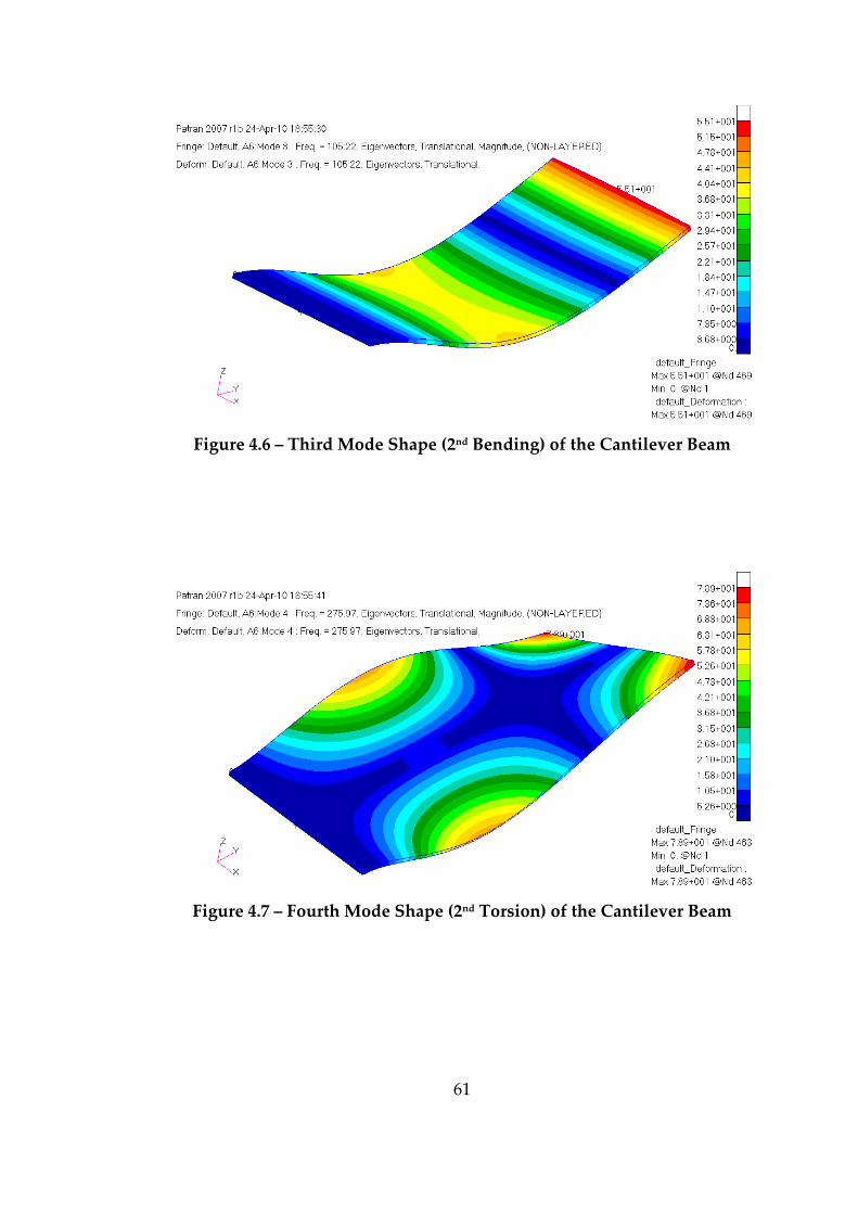
61
Figure 4.6 – Third Mode Shape (2nd Bending) of the Cantilever Beam
Figure 4.7 – Fourth Mode Shape (2nd Torsion) of the Cantilever Beam
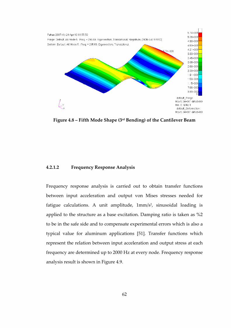
62
Figure 4.8 – Fifth Mode Shape (3rd Bending) of the Cantilever Beam
4.2.1.2 Frequency Response Analysis
Frequency response analysis is carried out to obtain transfer functions
between input acceleration and output von Mises stresses needed for
fatigue calculations. A unit amplitude, 1mm/s2, sinusoidal loading is
applied to the structure as a base excitation. Damping ratio is taken as %2
to be in the safe side and to compensate experimental errors which is also a
typical value for aluminum applications [51]. Transfer functions which
represent the relation between input acceleration and output stress at each
frequency are determined up to 2000 Hz at every node. Frequency response
analysis result is shown in Figure 4.9.
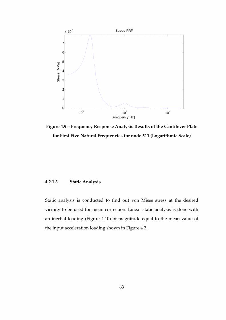
63
101 102 1030
1
2
3
4
5
6
7
x 10-4
Frequency[Hz]
Stre
ss [M
Pa]
Stress FRF
Figure 4.9 – Frequency Response Analysis Results of the Cantilever Plate
for First Five Natural Frequencies for node 511 (Logarithmic Scale)
4.2.1.3 Static Analysis
Static analysis is conducted to find out von Mises stress at the desired
vicinity to be used for mean correction. Linear static analysis is done with
an inertial loading (Figure 4.10) of magnitude equal to the mean value of
the input acceleration loading shown in Figure 4.2.
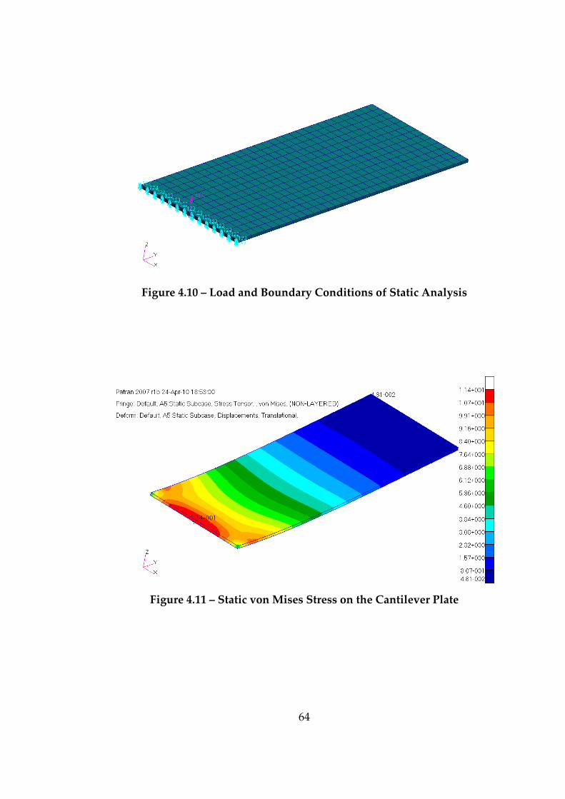
64
Figure 4.10 – Load and Boundary Conditions of Static Analysis
Figure 4.11 – Static von Mises Stress on the Cantilever Plate
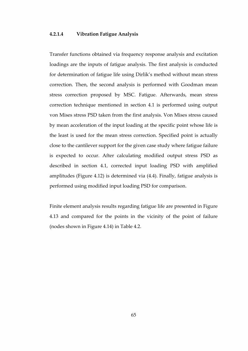
65
4.2.1.4 Vibration Fatigue Analysis
Transfer functions obtained via frequency response analysis and excitation
loadings are the inputs of fatigue analysis. The first analysis is conducted
for determination of fatigue life using Dirlik’s method without mean stress
correction. Then, the second analysis is performed with Goodman mean
stress correction proposed by MSC. Fatigue. Afterwards, mean stress
correction technique mentioned in section 4.1 is performed using output
von Mises stress PSD taken from the first analysis. Von Mises stress caused
by mean acceleration of the input loading at the specific point whose life is
the least is used for the mean stress correction. Specified point is actually
close to the cantilever support for the given case study where fatigue failure
is expected to occur. After calculating modified output stress PSD as
described in section 4.1, corrected input loading PSD with amplified
amplitudes (Figure 4.12) is determined via (4.4). Finally, fatigue analysis is
performed using modified input loading PSD for comparison.
Finite element analysis results regarding fatigue life are presented in Figure
4.13 and compared for the points in the vicinity of the point of failure
(nodes shown in Figure 4.14) in Table 4.2.
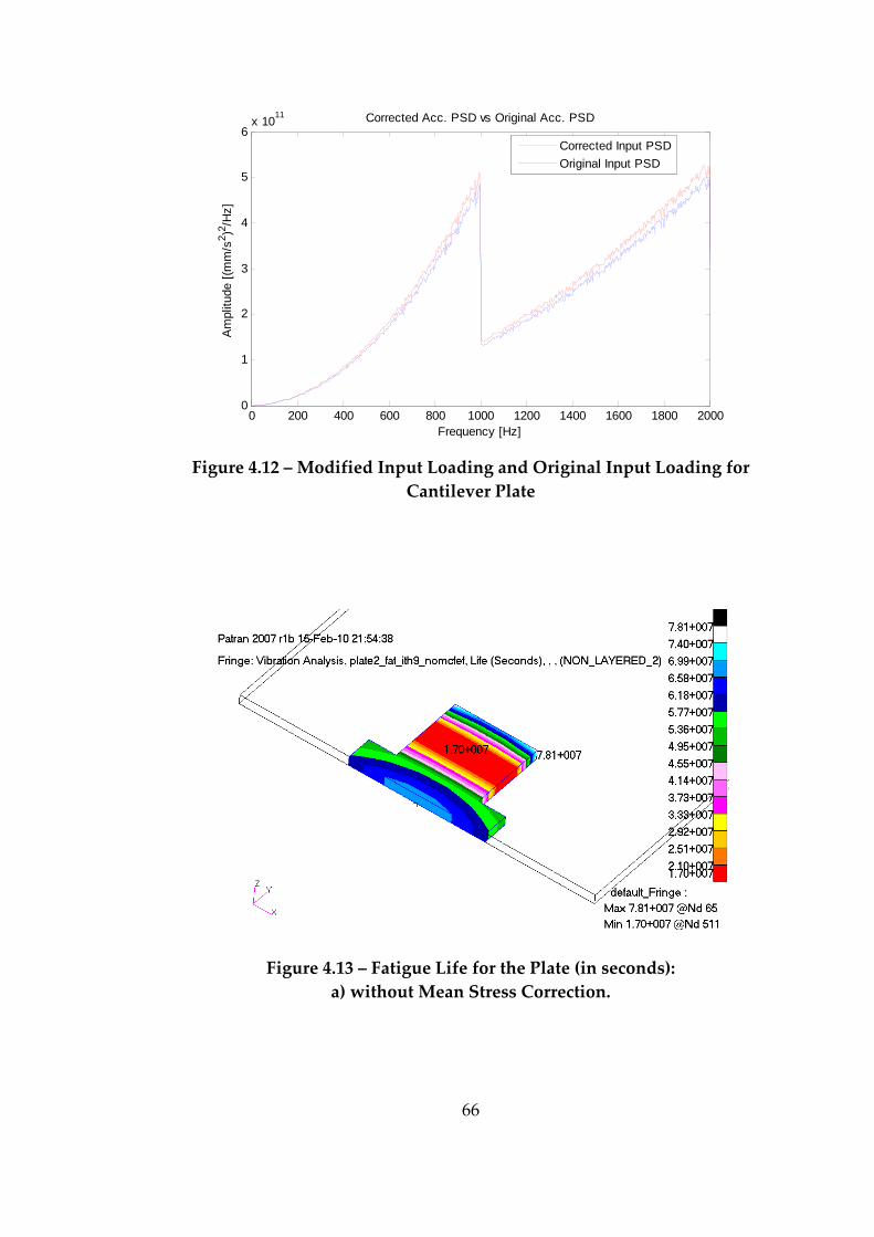
66
0 200 400 600 800 1000 1200 1400 1600 1800 20000
1
2
3
4
5
6x 10¹¹ Corrected Acc. PSD vs Original Acc. PSD
Frequency [Hz]
Am
plitu
de [(
mm
/s2 )2 /H
z]
Corrected Input PSDOriginal Input PSD
Figure 4.12 – Modified Input Loading and Original Input Loading for Cantilever Plate
Figure 4.13 – Fatigue Life for the Plate (in seconds): a) without Mean Stress Correction.
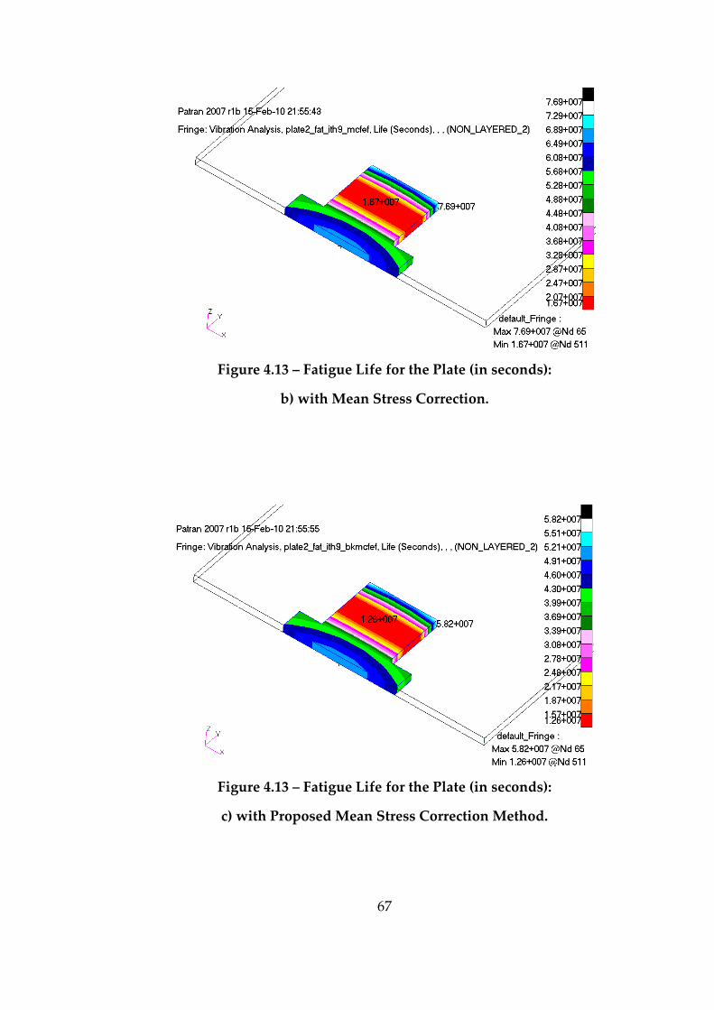
67
Figure 4.13 – Fatigue Life for the Plate (in seconds):
b) with Mean Stress Correction.
Figure 4.13 – Fatigue Life for the Plate (in seconds):
c) with Proposed Mean Stress Correction Method.
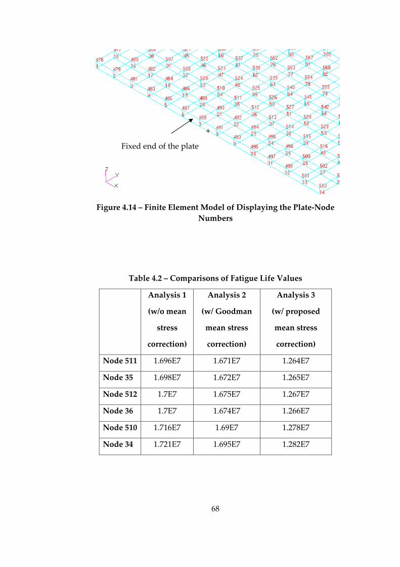
68
Figure 4.14 – Finite Element Model of Displaying the Plate‐Node Numbers
Table 4.2 – Comparisons of Fatigue Life Values
Analysis 1
(w/o mean
stress
correction)
Analysis 2
(w/ Goodman
mean stress
correction)
Analysis 3
(w/ proposed
mean stress
correction)
Node 511 1.696E7 1.671E7 1.264E7
Node 35 1.698E7 1.672E7 1.265E7
Node 512 1.7E7 1.675E7 1.267E7
Node 36 1.7E7 1.674E7 1.266E7
Node 510 1.716E7 1.69E7 1.278E7
Node 34 1.721E7 1.695E7 1.282E7
Fixed end of the plate

69
Developed method gives a more conservative fatigue life compared to that
obtained by the Goodman mean stress correction used in the MSC Fatigue
software. Therefore, the input loading obtained by means of the
aforementioned method is concluded to be safe, practical and convenient
for experimental applications.
70
CHAPTER 5
GENERATION OF A ZERO MEAN EXCITATION FOR MULTI‐AXIAL
LOADING
A machine component can be subjected to loadings in three axis
perpendicular to each other that have a nonzero mean value. Then, the
mean values appearing in loading sets will affect the stresses and thus the
fatigue life of the component. In this chapter, a method is proposed to
create a modified input loading set with zero mean which causes fatigue
damage approximately equivalent to that created by input loading set with
nonzero mean in three loading axis. For this purpose, a mathematical
procedure is developed to apply mean stress correction to the output stress
power spectral density matrix taking all stress components’ effect into
account. A modified input acceleration power spectral density matrix is
generated by means of transfer functions between input and output
calculated via frequency response analysis. This mathematical approach
considers the multi‐axial stresses at the point of interest and presents the
needed input loading power spectral density. The modified input with zero
mean value enables experimental verification while the mean value, other
than 1g, of the input cannot be applied with standard vibration
equipments.
The mean stress correction is accomplished with Goodman formula and
Dirlik method is applied as vibration fatigue life calculation technique.
71
It is revealed that the proposed technique is useful in creating a modified
input acceleration data set with a zero mean that can simulate the damage
for a selected point in the structure under consideration. Equivalent input
loading set is convenient and conservative for experimental applications.
The developed technique is a time saving and appropriate method to be
implemented for any type of loading.
Note that, some formulae and knowledge given in previous chapters are
repeated in this chapter for the sake of integrity of the work presented.
5.1 Theory
The modification method to calculate zero mean loading set, )( fGim , which
leads to approximately equivalent fatigue damage on a structure which is
subjected to a random loading with nonzero mean, is based on the
frequency domain fatigue calculation techniques.
The linear relation between the input and the output of the system which
are, in this chapter, acceleration, and stress, respectively, is given with (5.1)
in frequency domain. Transfer function matrix elements are in complex
form.
(5.1)
where { })( fa is acceleration vector, [ ])( fH is transfer function matrix and
{ })( fσ is stress vector given in (5.2), (5.3), (5.4), respectively.
{ } [ ]{ })()()( fafHf =σ
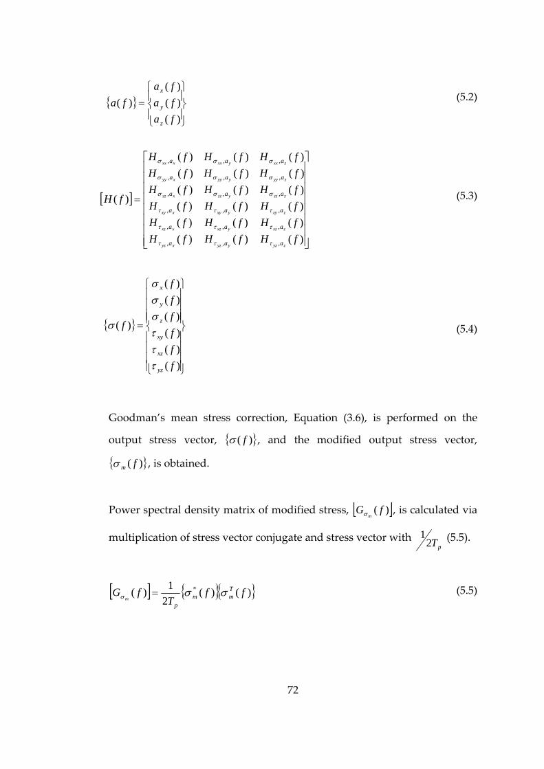
72
(5.2)
(5.3)
(5.4)
Goodman’s mean stress correction, Equation (3.6), is performed on the
output stress vector, { })( fσ , and the modified output stress vector,
{ })( fmσ , is obtained.
Power spectral density matrix of modified stress, [ ])( fGmσ , is calculated via
multiplication of stress vector conjugate and stress vector with pT2
1 (5.5).
(5.5)
{ }⎪⎭
⎪⎬
⎫
⎪⎩
⎪⎨
⎧=
)()()(
)(fafafa
fa
z
y
x
[ ]
⎥⎥⎥⎥⎥⎥⎥⎥
⎦
⎤
⎢⎢⎢⎢⎢⎢⎢⎢
⎣
⎡
=
)()()()()()()()()()()()()()()()()()(
)(
,,,
,,,
,,,
,,,
,,,
,,,
fHfHfHfHfHfHfHfHfHfHfHfHfHfHfHfHfHfH
fH
zyzyyzxyz
zxzyxzxxz
zxyyxyxxy
zzzyzzxzz
zyyyyyxyy
zxxyxxxxx
aaa
aaa
aaa
aaa
aaa
aaa
τττ
τττ
τττ
σσσ
σσσ
σσσ
{ }
⎪⎪⎪⎪
⎭
⎪⎪⎪⎪
⎬
⎫
⎪⎪⎪⎪
⎩
⎪⎪⎪⎪
⎨
⎧
=
)()()()()()(
)(
ffffff
f
yz
xz
xy
z
y
x
τττσσσ
σ
[ ] { }{ })()(2
1)( * ffT
fG Tmm
pm
σσσ =
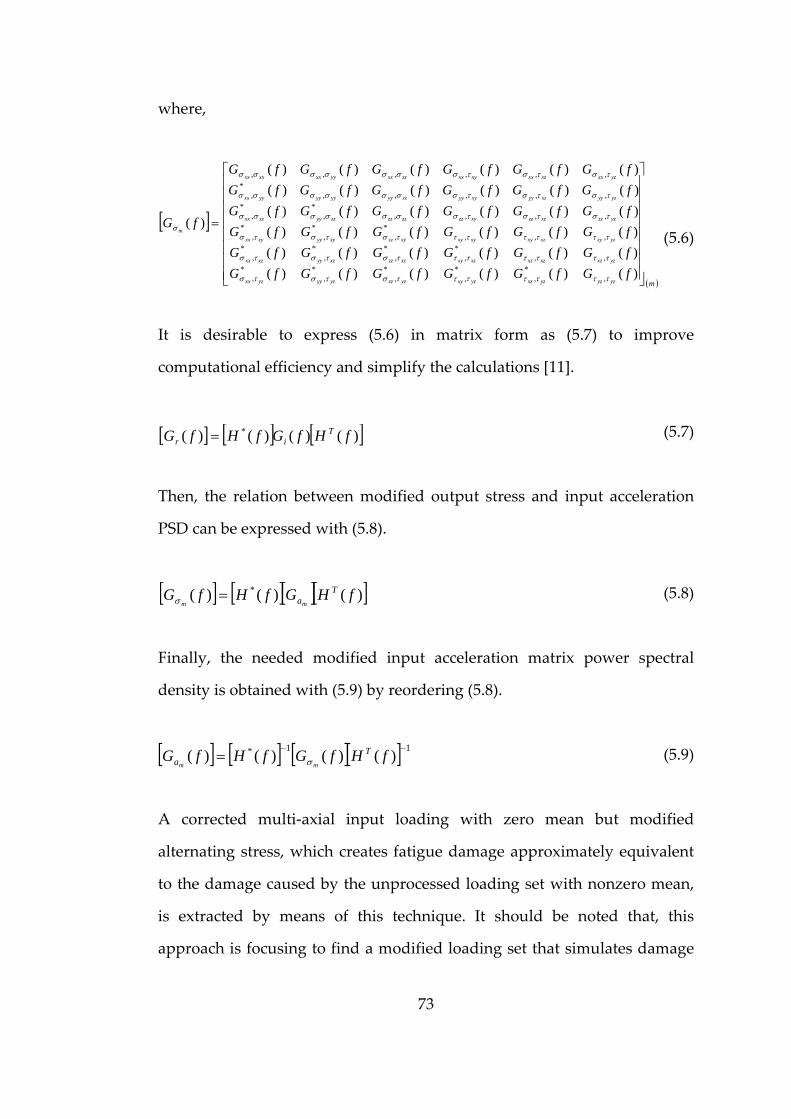
73
where,
(5.6)
It is desirable to express (5.6) in matrix form as (5.7) to improve
computational efficiency and simplify the calculations [11].
(5.7)
Then, the relation between modified output stress and input acceleration
PSD can be expressed with (5.8).
(5.8)
Finally, the needed modified input acceleration matrix power spectral
density is obtained with (5.9) by reordering (5.8).
(5.9)
A corrected multi‐axial input loading with zero mean but modified
alternating stress, which creates fatigue damage approximately equivalent
to the damage caused by the unprocessed loading set with nonzero mean,
is extracted by means of this technique. It should be noted that, this
approach is focusing to find a modified loading set that simulates damage
[ ]
( )mfGfGfGfGfGfGfGfGfGfGfGfGfGfGfGfGfGfGfGfGfGfGfGfGfGfGfGfGfGfGfGfGfGfGfGfG
fG
yzyzyzxzyzxyyzzzyzyyyzxx
yzxzxzxzxzxyxzzzxzyyxzxx
yzxyxzxyxyxyxyzzxyyyxyxx
yzzzxzzzxyzzzzzzzzyyzzxx
yzyyxzyyxyyyzzyyyyyyyyxx
yzxxxzxxxyxxzzxxyyxxxxxx
m
⎥⎥⎥⎥⎥⎥⎥⎥
⎦
⎤
⎢⎢⎢⎢⎢⎢⎢⎢
⎣
⎡
=
)()()()()()()()()()()()()()()()()()()()()()()()()()()()()()()()()()()()(
)(
,*
,*
,*
,*
,*
,
,,*
,*
,*
,*
,
,,,*
,*
,*
,
,,,,*
,*
,
,,,,,*
,
,,,,,,
τττττττστστσ
τττττττστστσ
τττττττστστσ
τστστσσσσσσσ
τστστσσσσσσσ
τστστσσσσσσσ
σ
[ ] [ ][ ][ ])()()( * fHGfHfG Tamm
=σ
[ ] [ ] [ ])()()()( * fHfGfHfG Tir =
[ ] [ ] [ ][ ] 11* )()()()( −−= fHfGfHfG T
a mm σ

74
for a selected point on the structure, which in turn will be acceptable in the
vicinity of that point only.
5.2 Case Studies
5.2.1 Case Study I – Test Comparison
In this case study it is aimed to compare the proposed input loading
generation method with test results. For this purpose a notched specimen is
used since there would be lengthy test durations needed otherwise.
The dimensions of the 3 mm thick test specimen are given in Figure 5.1
with respect to the clamped end. The test specimen is manufactured from
aluminum 5754 H111.
Figure 5.1 – Dimensions of the test specimen (Dimensions in [mm])

75
Standard vibration test systems do not have capabilities which enable mean
stress application. Therefore a mean value of 1 g in the acceleration
excitation is selected since it can be applied if the excitation direction is
selected as vertical to make use of Earth’s gravity.
Hence, tests are conducted in 2 different configurations. The first
configuration is used for the actual mean stress test on a vertical vibration
shaker armature as shown in Figure 5.2. The second configuration, shown
in Figure 5.3 where a horizontal vibration shaker and slip table system is
utilized, is used for both the pure alternating test and the test where
modified loading corresponding to the proposed mean stress correction
method is applied.
For these three tests, corresponding analysis are also conducted. Note that
for the horizontal test condition, there is a 1 g mean stress acting in a
direction perpendicular to the excitation direction. To show that this
perpendicular mean stress does not affect the results critically, for the pure
alternating test, another analysis is performed where this perpendicular
mean stress is also taken into account. It is observed that the life reduction
is less than %0.5 so the effect is negligible.
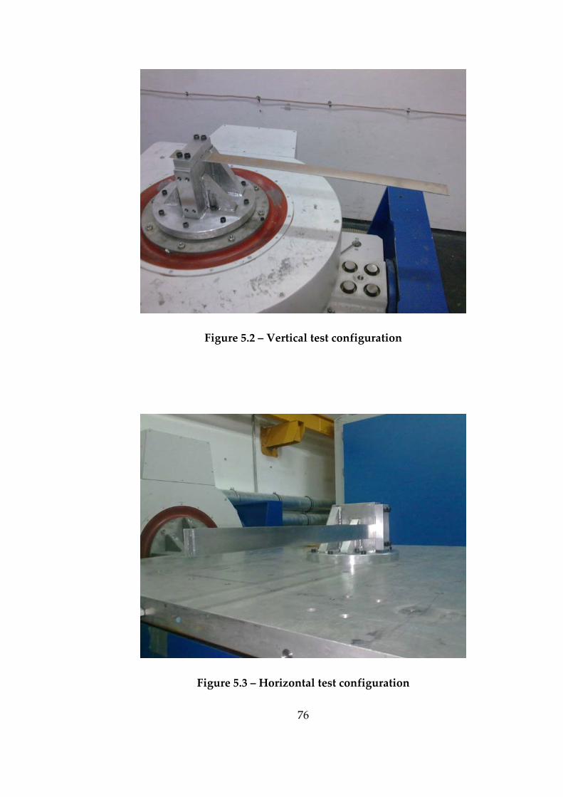
76
Figure 5.2 – Vertical test configuration
Figure 5.3 – Horizontal test configuration
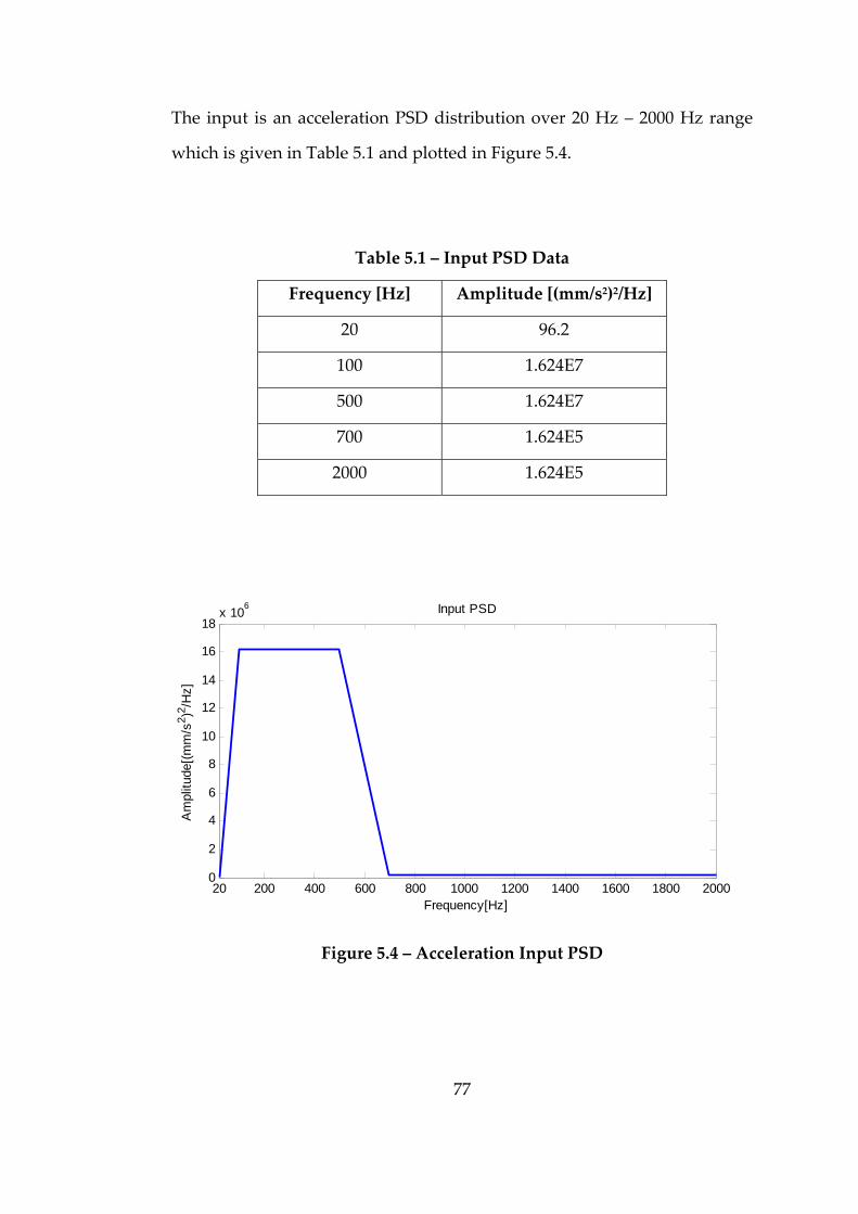
77
The input is an acceleration PSD distribution over 20 Hz – 2000 Hz range
which is given in Table 5.1 and plotted in Figure 5.4.
Table 5.1 – Input PSD Data
Frequency [Hz] Amplitude [(mm/s2)2/Hz]
20 96.2
100 1.624E7
500 1.624E7
700 1.624E5
2000 1.624E5
20 200 400 600 800 1000 1200 1400 1600 1800 20000
2
4
6
8
10
12
14
16
18x 106 Input PSD
Frequency[Hz]
Am
plitu
de[(m
m/s
2 )2 /Hz]
Figure 5.4 – Acceleration Input PSD
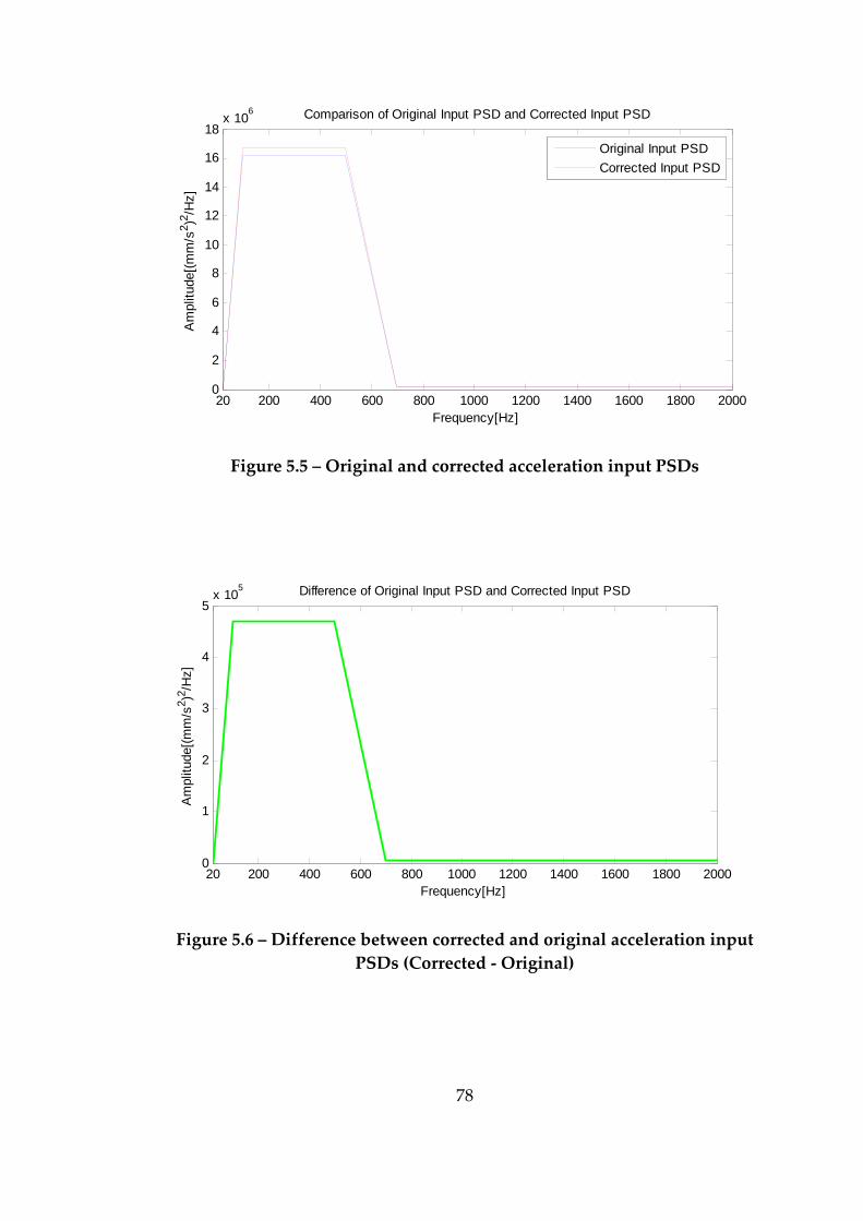
78
20 200 400 600 800 1000 1200 1400 1600 1800 20000
2
4
6
8
10
12
14
16
18x 106 Comparison of Original Input PSD and Corrected Input PSD
Frequency[Hz]
Am
plitu
de[(m
m/s
2 )2 /Hz]
Original Input PSDCorrected Input PSD
Figure 5.5 – Original and corrected acceleration input PSDs
20 200 400 600 800 1000 1200 1400 1600 1800 20000
1
2
3
4
5x 10⁵ Difference of Original Input PSD and Corrected Input PSD
Frequency[Hz]
Am
plitu
de[(m
m/s
2 )2 /Hz]
Figure 5.6 – Difference between corrected and original acceleration input PSDs (Corrected ‐ Original)
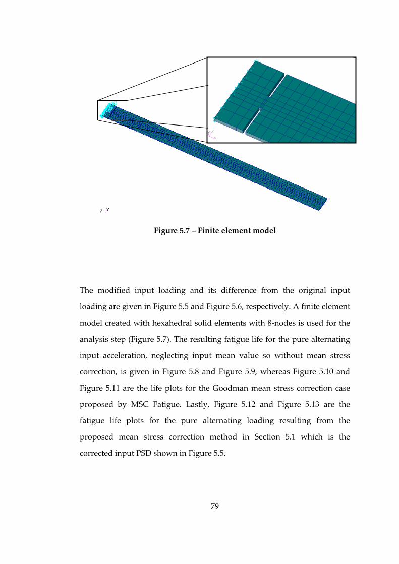
79
Figure 5.7 – Finite element model
The modified input loading and its difference from the original input
loading are given in Figure 5.5 and Figure 5.6, respectively. A finite element
model created with hexahedral solid elements with 8‐nodes is used for the
analysis step (Figure 5.7). The resulting fatigue life for the pure alternating
input acceleration, neglecting input mean value so without mean stress
correction, is given in Figure 5.8 and Figure 5.9, whereas Figure 5.10 and
Figure 5.11 are the life plots for the Goodman mean stress correction case
proposed by MSC Fatigue. Lastly, Figure 5.12 and Figure 5.13 are the
fatigue life plots for the pure alternating loading resulting from the
proposed mean stress correction method in Section 5.1 which is the
corrected input PSD shown in Figure 5.5.
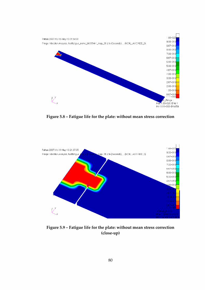
80
Figure 5.8 – Fatigue life for the plate: without mean stress correction
Figure 5.9 – Fatigue life for the plate: without mean stress correction (close‐up)
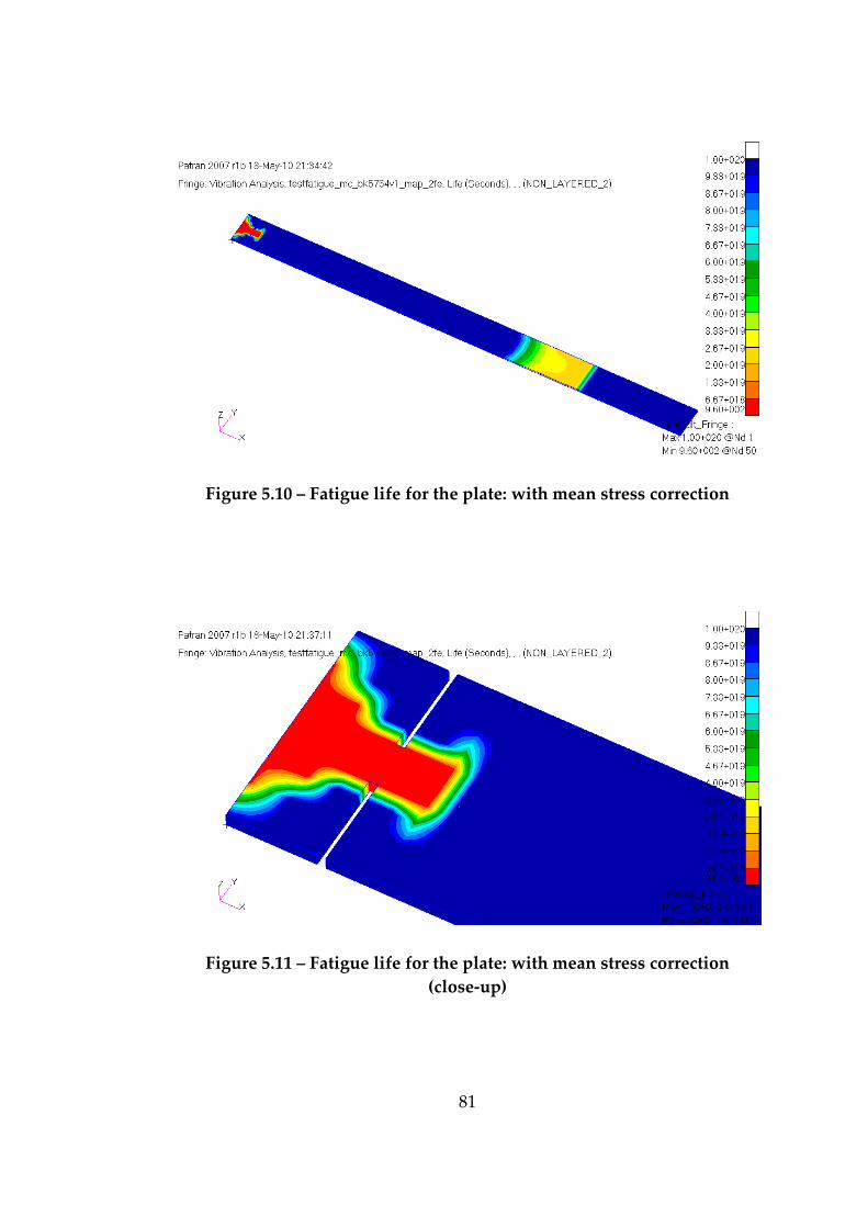
81
Figure 5.10 – Fatigue life for the plate: with mean stress correction
Figure 5.11 – Fatigue life for the plate: with mean stress correction (close‐up)
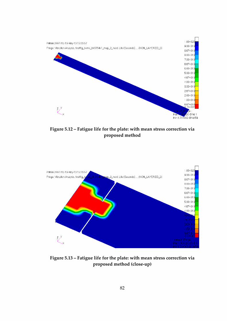
82
Figure 5.12 – Fatigue life for the plate: with mean stress correction via proposed method
Figure 5.13 – Fatigue life for the plate: with mean stress correction via proposed method (close‐up)
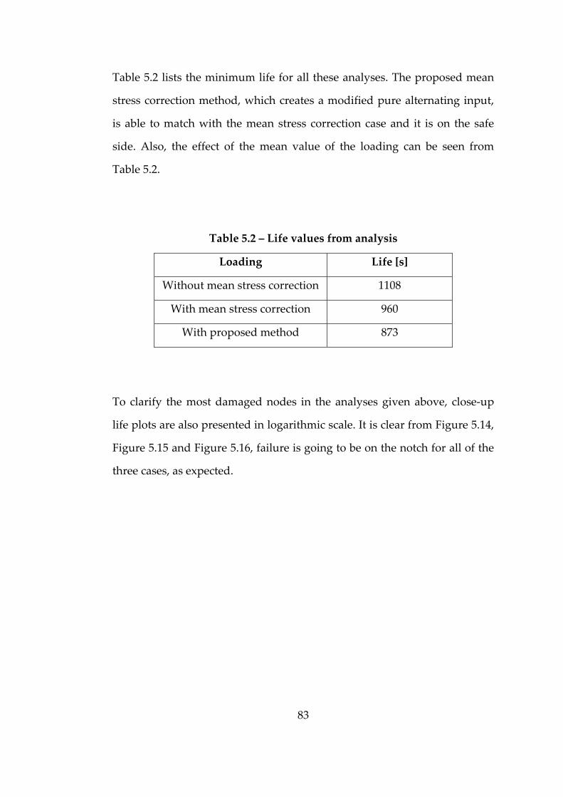
83
Table 5.2 lists the minimum life for all these analyses. The proposed mean
stress correction method, which creates a modified pure alternating input,
is able to match with the mean stress correction case and it is on the safe
side. Also, the effect of the mean value of the loading can be seen from
Table 5.2.
Table 5.2 – Life values from analysis
Loading Life [s]
Without mean stress correction 1108
With mean stress correction 960
With proposed method 873
To clarify the most damaged nodes in the analyses given above, close‐up
life plots are also presented in logarithmic scale. It is clear from Figure 5.14,
Figure 5.15 and Figure 5.16, failure is going to be on the notch for all of the
three cases, as expected.
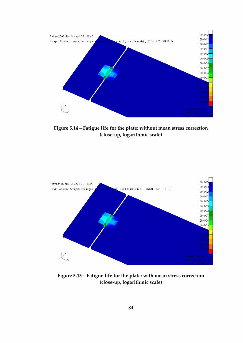
84
Figure 5.14 – Fatigue life for the plate: without mean stress correction (close‐up, logarithmic scale)
Figure 5.15 – Fatigue life for the plate: with mean stress correction (close‐up, logarithmic scale)
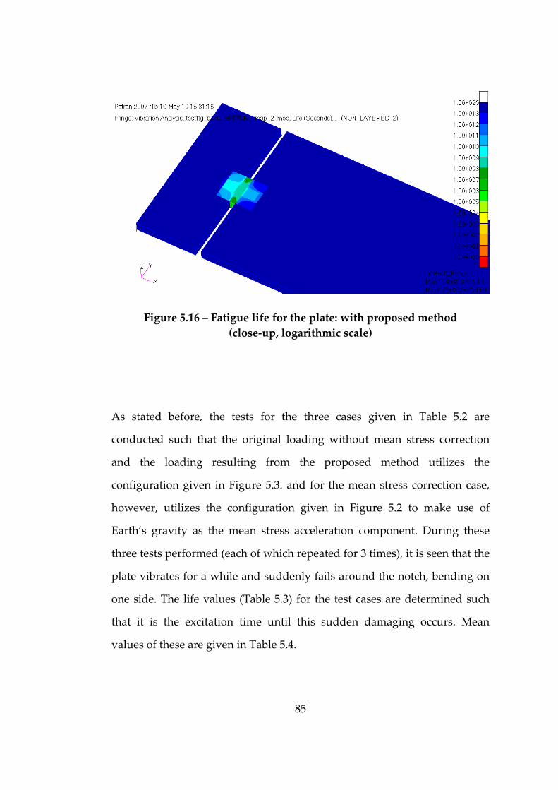
85
Figure 5.16 – Fatigue life for the plate: with proposed method (close‐up, logarithmic scale)
As stated before, the tests for the three cases given in Table 5.2 are
conducted such that the original loading without mean stress correction
and the loading resulting from the proposed method utilizes the
configuration given in Figure 5.3. and for the mean stress correction case,
however, utilizes the configuration given in Figure 5.2 to make use of
Earth’s gravity as the mean stress acceleration component. During these
three tests performed (each of which repeated for 3 times), it is seen that the
plate vibrates for a while and suddenly fails around the notch, bending on
one side. The life values (Table 5.3) for the test cases are determined such
that it is the excitation time until this sudden damaging occurs. Mean
values of these are given in Table 5.4.
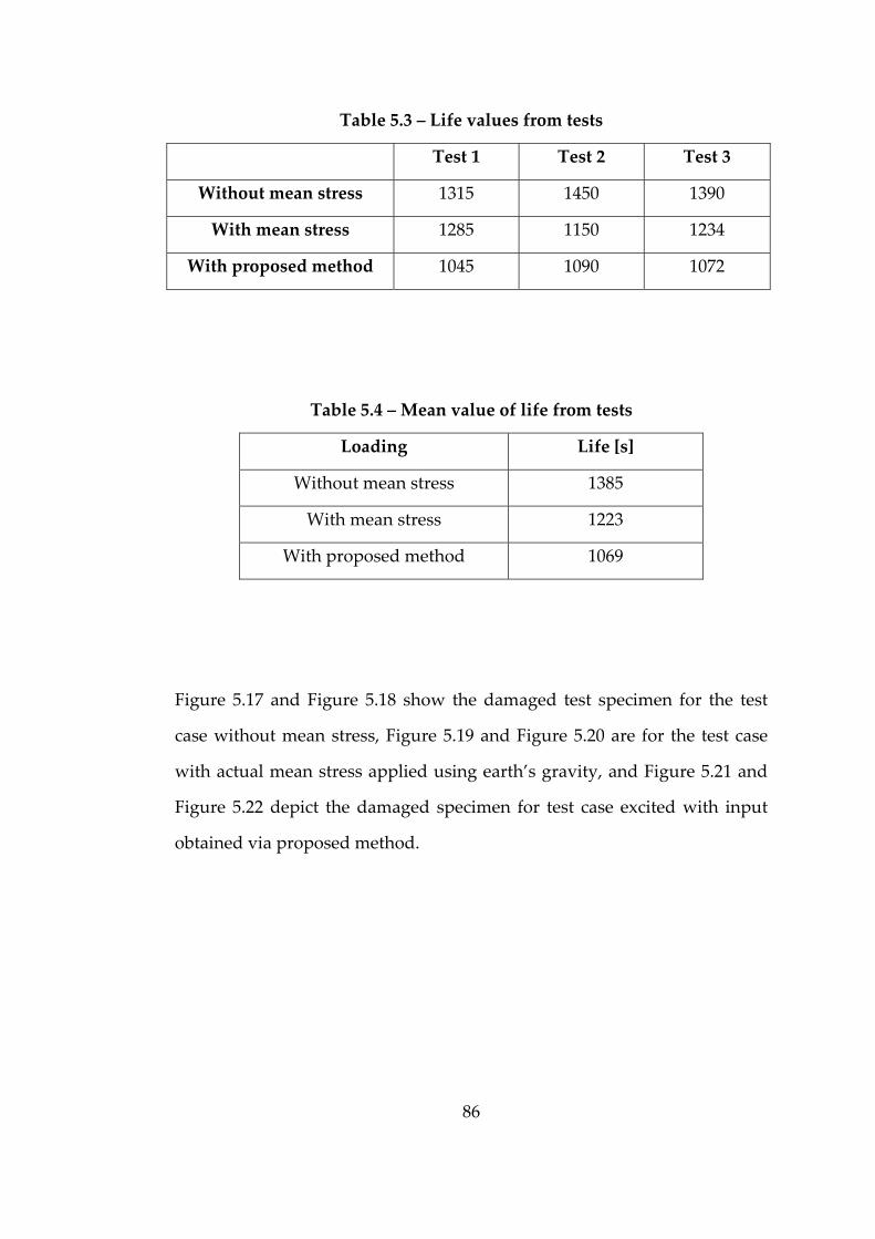
86
Table 5.3 – Life values from tests
Test 1 Test 2 Test 3
Without mean stress 1315 1450 1390
With mean stress 1285 1150 1234
With proposed method 1045 1090 1072
Table 5.4 – Mean value of life from tests
Loading Life [s]
Without mean stress 1385
With mean stress 1223
With proposed method 1069
Figure 5.17 and Figure 5.18 show the damaged test specimen for the test
case without mean stress, Figure 5.19 and Figure 5.20 are for the test case
with actual mean stress applied using earth’s gravity, and Figure 5.21 and
Figure 5.22 depict the damaged specimen for test case excited with input
obtained via proposed method.
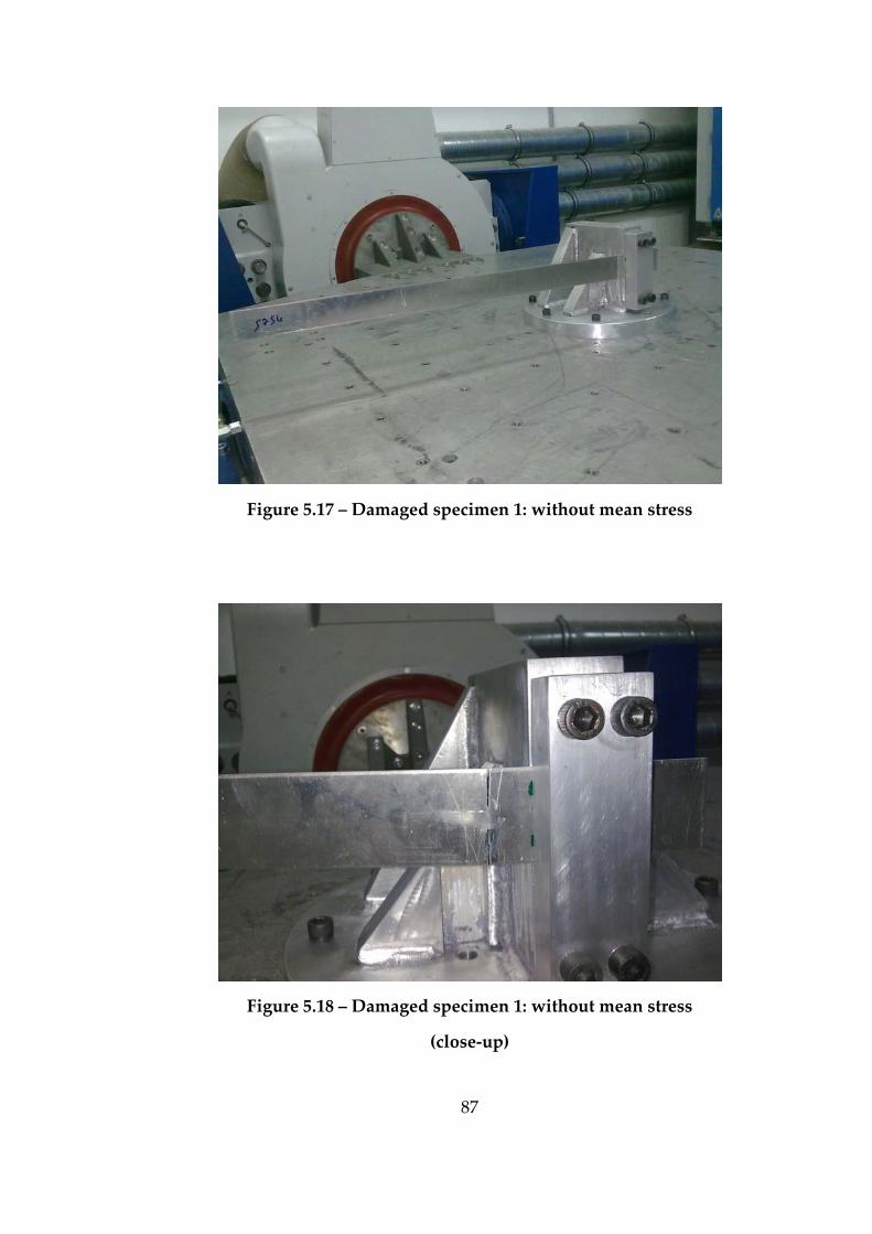
87
Figure 5.17 – Damaged specimen 1: without mean stress
Figure 5.18 – Damaged specimen 1: without mean stress
(close‐up)
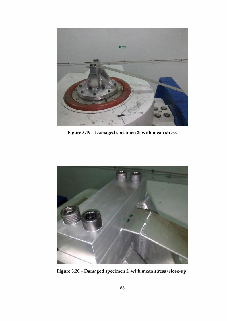
88
Figure 5.19 – Damaged specimen 2: with mean stress
Figure 5.20 – Damaged specimen 2: with mean stress (close‐up)
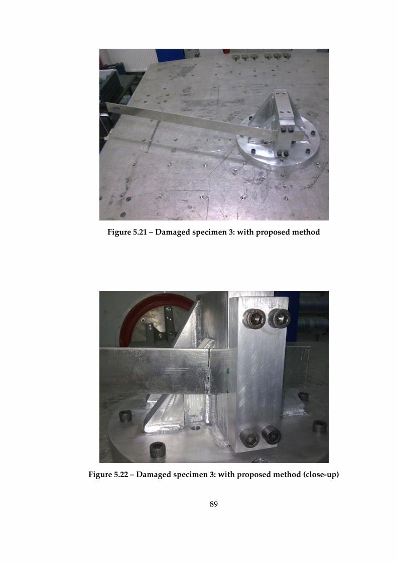
89
Figure 5.21 – Damaged specimen 3: with proposed method
Figure 5.22 – Damaged specimen 3: with proposed method (close‐up)
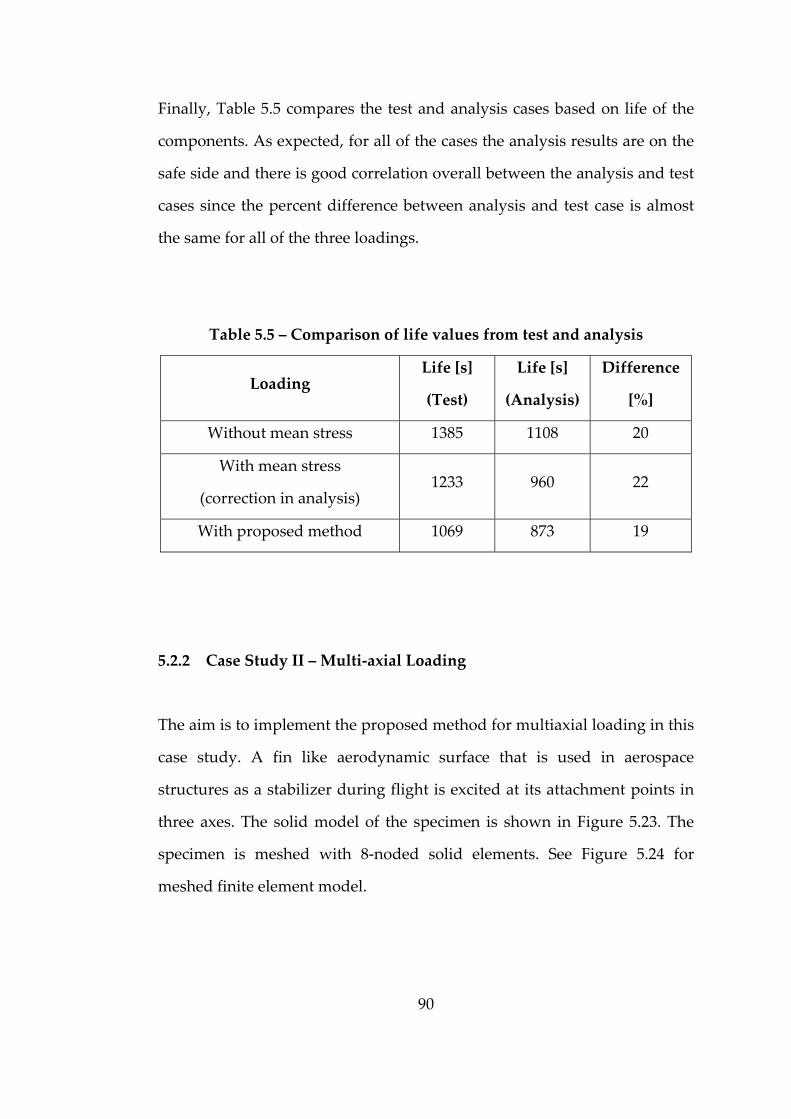
90
Finally, Table 5.5 compares the test and analysis cases based on life of the
components. As expected, for all of the cases the analysis results are on the
safe side and there is good correlation overall between the analysis and test
cases since the percent difference between analysis and test case is almost
the same for all of the three loadings.
Table 5.5 – Comparison of life values from test and analysis
Loading Life [s]
(Test)
Life [s]
(Analysis)
Difference
[%]
Without mean stress 1385 1108 20
With mean stress
(correction in analysis) 1233 960 22
With proposed method 1069 873 19
5.2.2 Case Study II – Multi‐axial Loading
The aim is to implement the proposed method for multiaxial loading in this
case study. A fin like aerodynamic surface that is used in aerospace
structures as a stabilizer during flight is excited at its attachment points in
three axes. The solid model of the specimen is shown in Figure 5.23. The
specimen is meshed with 8‐noded solid elements. See Figure 5.24 for
meshed finite element model.
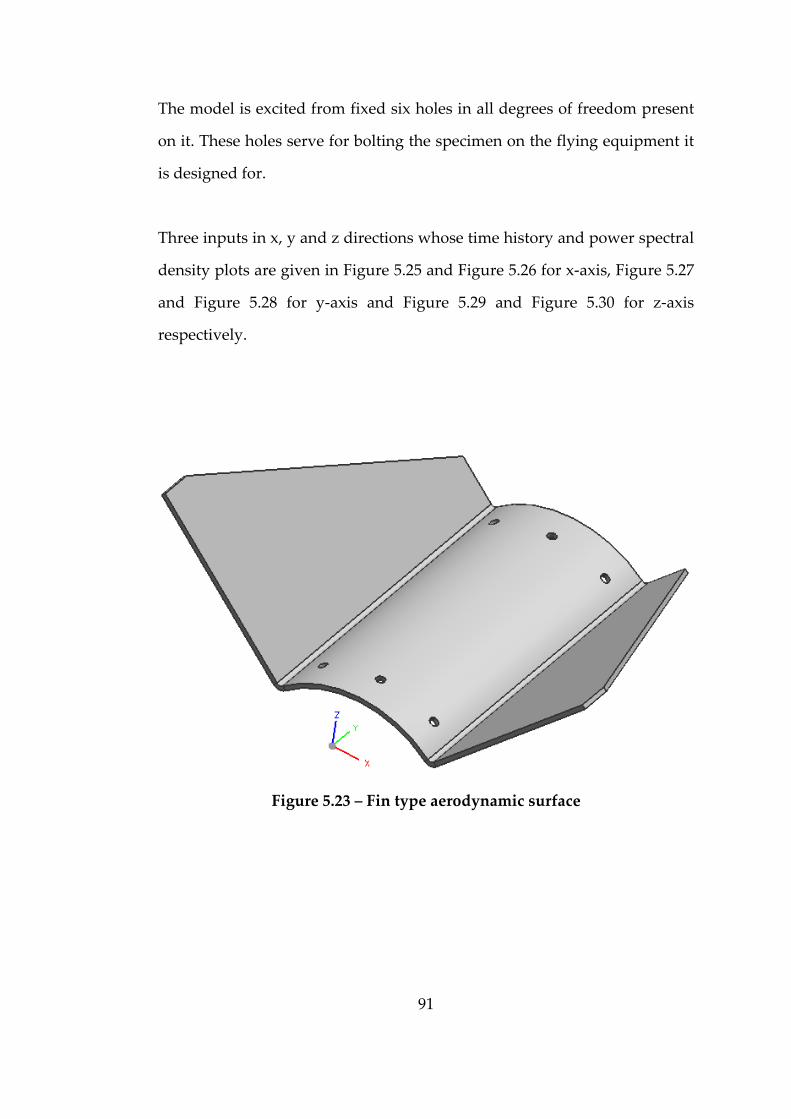
91
The model is excited from fixed six holes in all degrees of freedom present
on it. These holes serve for bolting the specimen on the flying equipment it
is designed for.
Three inputs in x, y and z directions whose time history and power spectral
density plots are given in Figure 5.25 and Figure 5.26 for x‐axis, Figure 5.27
and Figure 5.28 for y‐axis and Figure 5.29 and Figure 5.30 for z‐axis
respectively.
Figure 5.23 – Fin type aerodynamic surface
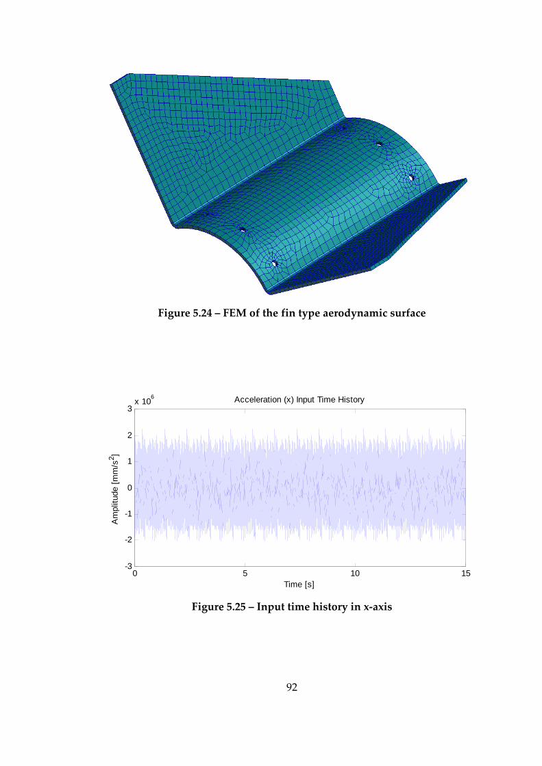
92
Figure 5.24 – FEM of the fin type aerodynamic surface
0 5 10 15-3
-2
-1
0
1
2
3x 10⁶ Acceleration (x) Input Time History
Time [s]
Am
plitu
de [m
m/s
2 ]
Figure 5.25 – Input time history in x‐axis
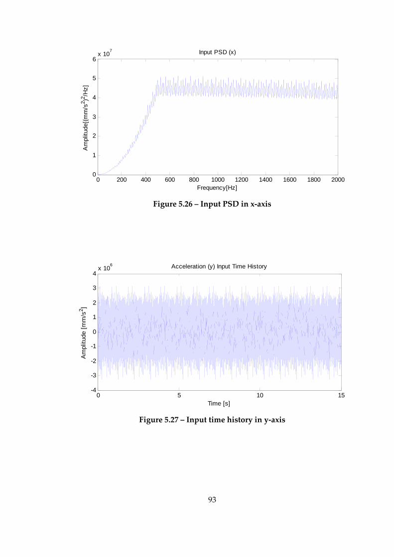
93
0 200 400 600 800 1000 1200 1400 1600 1800 20000
1
2
3
4
5
6x 10⁷ Input PSD (x)
Frequency[Hz]
Am
plitu
de[(m
m/s
2 )2 /Hz]
Figure 5.26 – Input PSD in x‐axis
0 5 10 15-4
-3
-2
-1
0
1
2
3
4x 10⁶ Acceleration (y) Input Time History
Time [s]
Am
plitu
de [m
m/s
2 ]
Figure 5.27 – Input time history in y‐axis
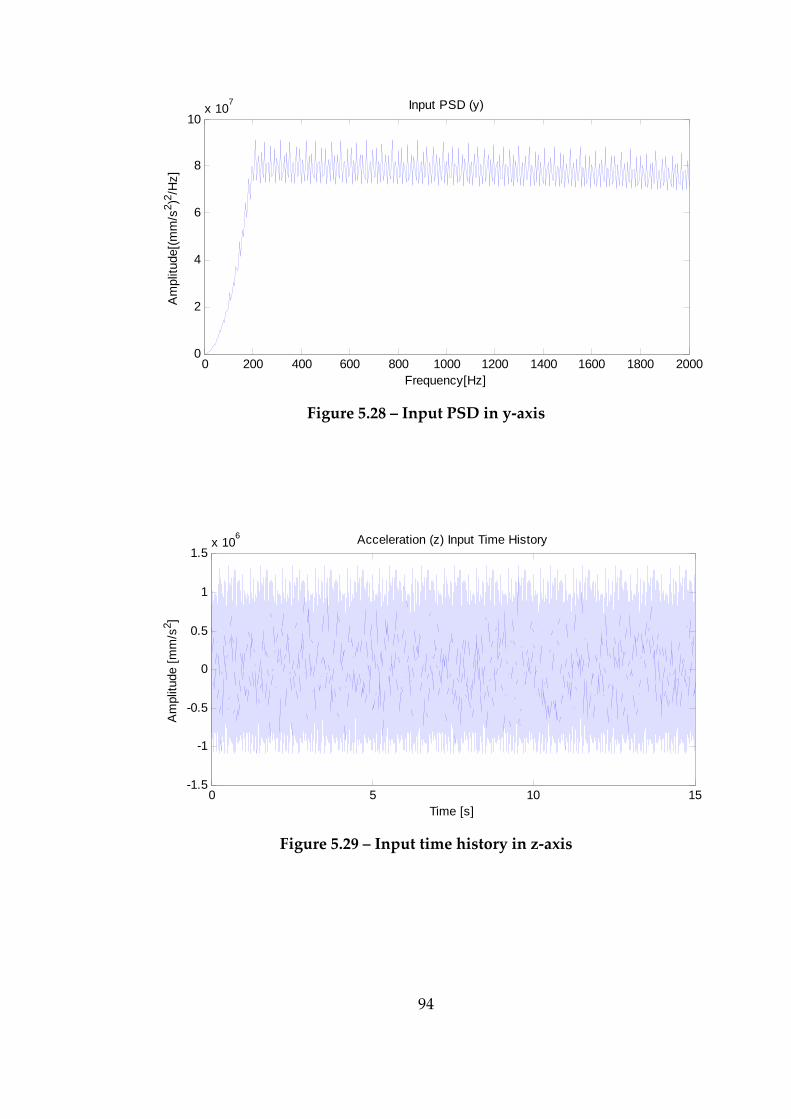
94
0 200 400 600 800 1000 1200 1400 1600 1800 20000
2
4
6
8
10x 107 Input PSD (y)
Frequency[Hz]
Am
plitu
de[(m
m/s
2 )2 /Hz]
Figure 5.28 – Input PSD in y‐axis
0 5 10 15-1.5
-1
-0.5
0
0.5
1
1.5x 10
6 Acceleration (z) Input Time History
Time [s]
Am
plitu
de [m
m/s
2 ]
Figure 5.29 – Input time history in z‐axis
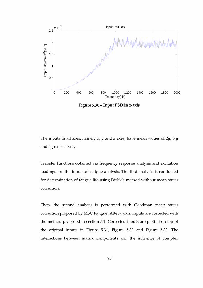
95
0 200 400 600 800 1000 1200 1400 1600 1800 20000
0.5
1
1.5
2
2.5x 10⁷ Input PSD (z)
Frequency[Hz]
Am
plitu
de[(m
m/s
2 )2 /Hz]
Figure 5.30 – Input PSD in z‐axis
The inputs in all axes, namely x, y and z axes, have mean values of 2g, 3 g
and 4g respectively.
Transfer functions obtained via frequency response analysis and excitation
loadings are the inputs of fatigue analysis. The first analysis is conducted
for determination of fatigue life using Dirlik’s method without mean stress
correction.
Then, the second analysis is performed with Goodman mean stress
correction proposed by MSC Fatigue. Afterwards, inputs are corrected with
the method proposed in section 5.1. Corrected inputs are plotted on top of
the original inputs in Figure 5.31, Figure 5.32 and Figure 5.33. The
interactions between matrix components and the influence of complex
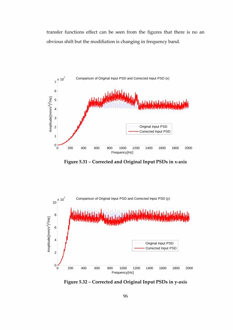
96
transfer functions effect can be seen from the figures that there is no an
obvious shift but the modifiation is changing in frequency band.
0 200 400 600 800 1000 1200 1400 1600 1800 20000
1
2
3
4
5
6
7x 10
7 Comparison of Original Input PSD and Corrected Input PSD (x)
Frequency[Hz]
Am
plitu
de[(m
m/s
2 )2 /Hz]
Original Input PSDCorrected Input PSD
Figure 5.31 – Corrected and Original Input PSDs in x‐axis
0 200 400 600 800 1000 1200 1400 1600 1800 20000
2
4
6
8
10x 107 Comparison of Original Input PSD and Corrected Input PSD (y)
Frequency[Hz]
Am
plitu
de[(m
m/s
2 )2 /Hz]
Original Input PSDCorrected Input PSD
Figure 5.32 – Corrected and Original Input PSDs in y‐axis
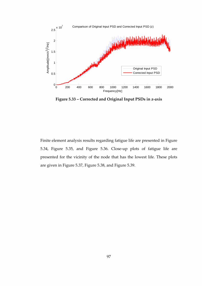
97
0 200 400 600 800 1000 1200 1400 1600 1800 20000
0.5
1
1.5
2
2.5x 10⁷ Comparison of Original Input PSD and Corrected Input PSD (z)
Frequency[Hz]
Am
plitu
de[(m
m/s
2 )2 /Hz]
Original Input PSDCorrected Input PSD
Figure 5.33 – Corrected and Original Input PSDs in z‐axis
Finite element analysis results regarding fatigue life are presented in Figure
5.34, Figure 5.35, and Figure 5.36. Close‐up plots of fatigue life are
presented for the vicinity of the node that has the lowest life. These plots
are given in Figure 5.37, Figure 5.38, and Figure 5.39.
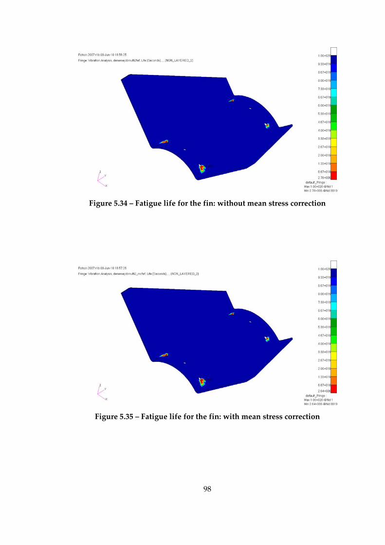
98
Figure 5.34 – Fatigue life for the fin: without mean stress correction
Figure 5.35 – Fatigue life for the fin: with mean stress correction
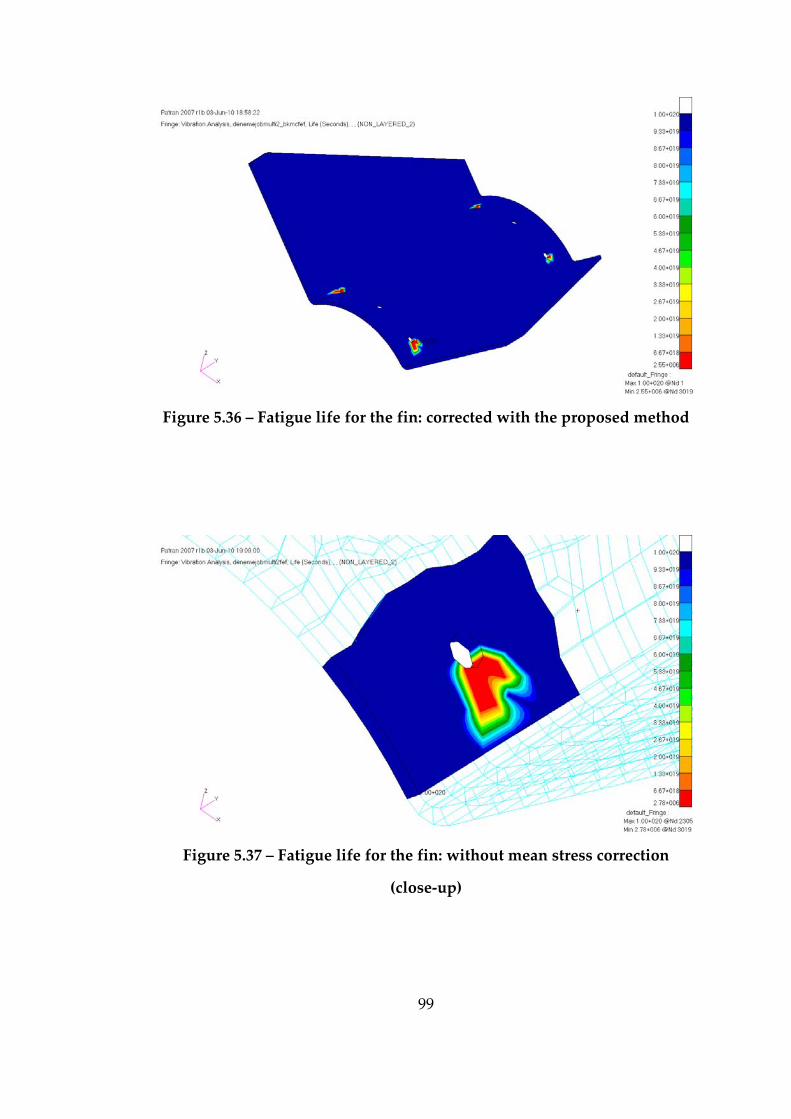
99
Figure 5.36 – Fatigue life for the fin: corrected with the proposed method
Figure 5.37 – Fatigue life for the fin: without mean stress correction
(close‐up)
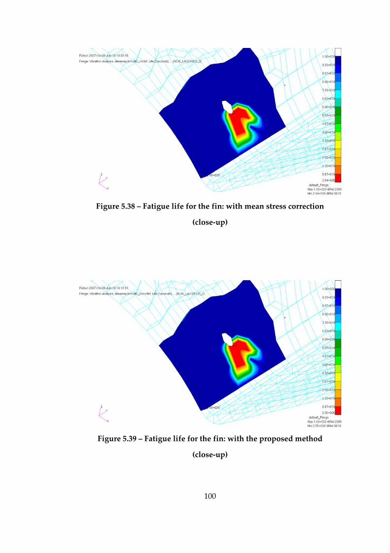
100
Figure 5.38 – Fatigue life for the fin: with mean stress correction
(close‐up)
Figure 5.39 – Fatigue life for the fin: with the proposed method
(close‐up)

101
In this case study it is shown that the developed method is able to take care
of multiaxial simultaneous inputs and yet gives a conservative fatigue life
and comparable result considering that obtained by the Goodman mean
stress correction.

102
CHAPTER 6
CONCLUSIONS AND DISCUSSION
In this thesis, vibration fatigue theory and its applications are examined.
When the loading is dynamic and randomly fluctuating consisting of sine
functions whose frequency content has a wide bandwidth, the resonance
frequencies of the structure are likely to be excited under dynamic loading.
Therefore, frequency domain fatigue analysis techniques are used in the
investigation of such situations that consider the dynamic response of the
structure.
In this study, fatigue theory is investigated in a chronological order and
vibration fatigue approaches proposed up to now are presented. Narrow
band solutions’ theories and how to develop broadband solution technique
are examined. Dirlik method is chosen as the broadband solution for
vibration fatigue calculations. It is a well known approach and commonly
used when the loading spectra has a wide bandwidth. It is easy to apply
and time saving. Rainflow counting is applied to identify stress ranges and
Goodman formula is used where mean stress correction is necessary
throughout this thesis.
A method is developed throughout the thesis study to create a modified
input loading history with zero mean value which leads to fatigue damage
approximately equivalent to that created by input loading with a nonzero
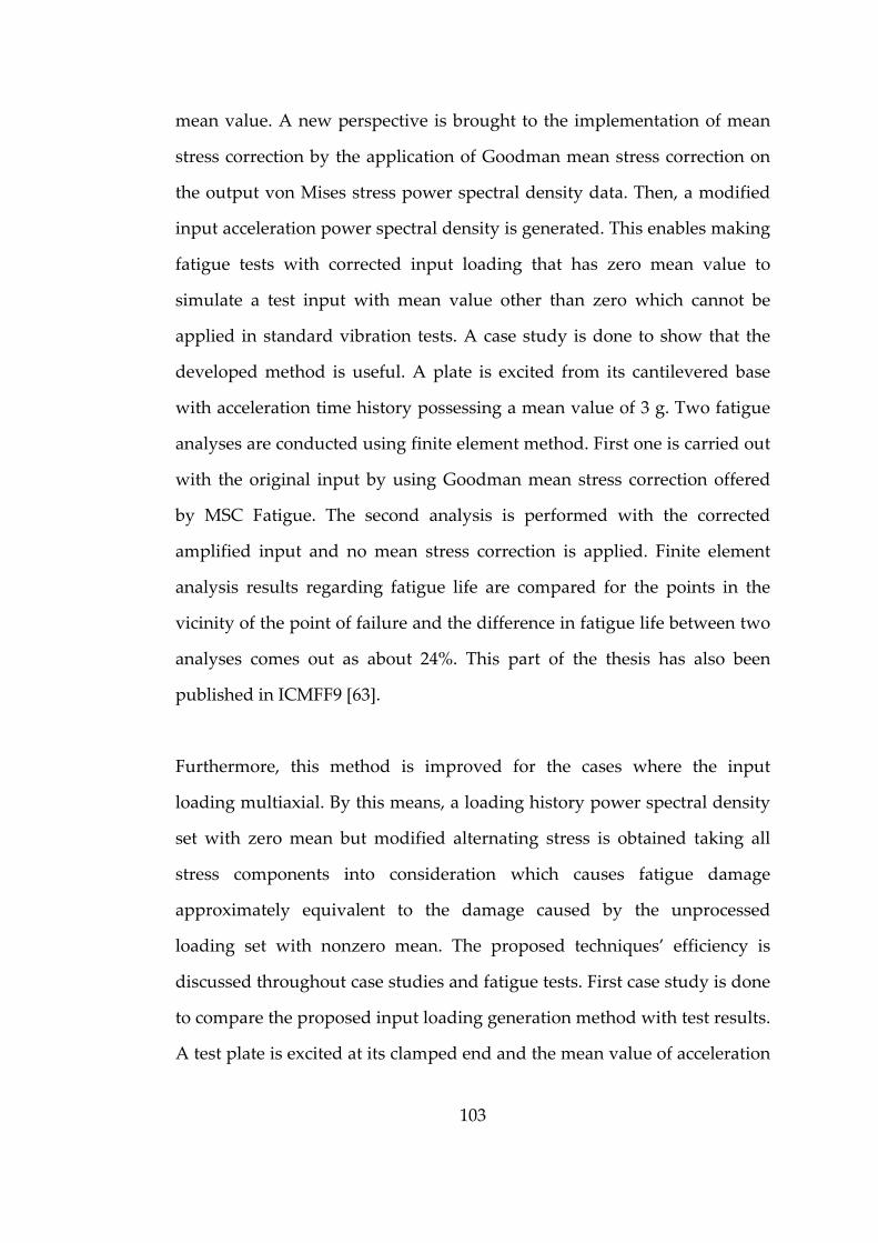
103
mean value. A new perspective is brought to the implementation of mean
stress correction by the application of Goodman mean stress correction on
the output von Mises stress power spectral density data. Then, a modified
input acceleration power spectral density is generated. This enables making
fatigue tests with corrected input loading that has zero mean value to
simulate a test input with mean value other than zero which cannot be
applied in standard vibration tests. A case study is done to show that the
developed method is useful. A plate is excited from its cantilevered base
with acceleration time history possessing a mean value of 3 g. Two fatigue
analyses are conducted using finite element method. First one is carried out
with the original input by using Goodman mean stress correction offered
by MSC Fatigue. The second analysis is performed with the corrected
amplified input and no mean stress correction is applied. Finite element
analysis results regarding fatigue life are compared for the points in the
vicinity of the point of failure and the difference in fatigue life between two
analyses comes out as about 24%. This part of the thesis has also been
published in ICMFF9 [63].
Furthermore, this method is improved for the cases where the input
loading multiaxial. By this means, a loading history power spectral density
set with zero mean but modified alternating stress is obtained taking all
stress components into consideration which causes fatigue damage
approximately equivalent to the damage caused by the unprocessed
loading set with nonzero mean. The proposed techniques’ efficiency is
discussed throughout case studies and fatigue tests. First case study is done
to compare the proposed input loading generation method with test results.
A test plate is excited at its clamped end and the mean value of acceleration
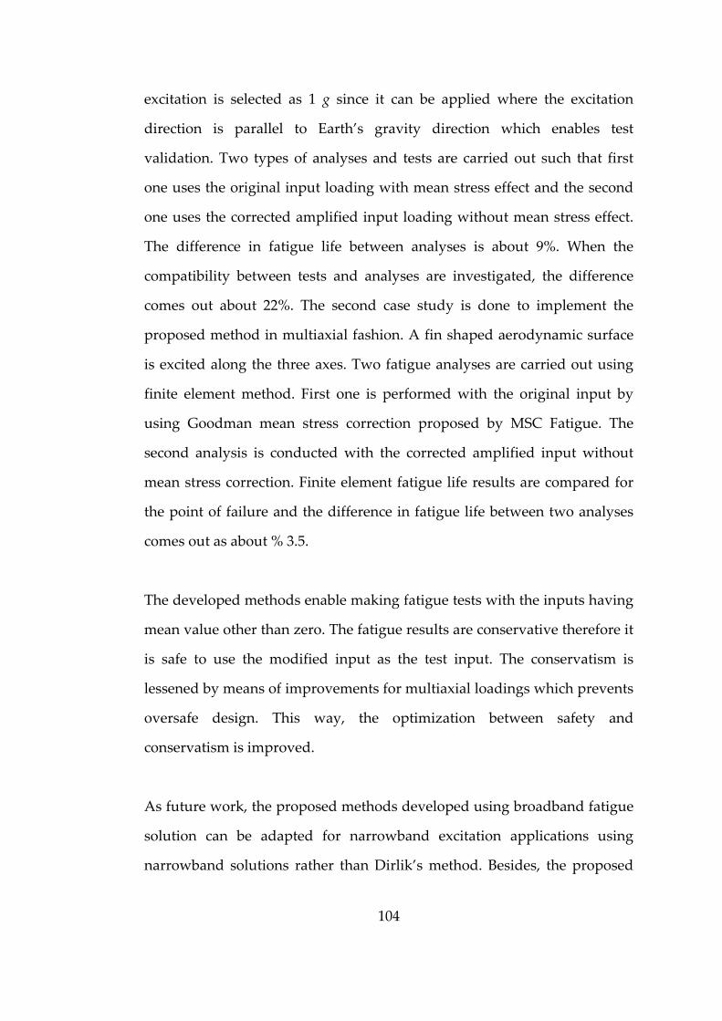
104
excitation is selected as 1 g since it can be applied where the excitation
direction is parallel to Earth’s gravity direction which enables test
validation. Two types of analyses and tests are carried out such that first
one uses the original input loading with mean stress effect and the second
one uses the corrected amplified input loading without mean stress effect.
The difference in fatigue life between analyses is about 9%. When the
compatibility between tests and analyses are investigated, the difference
comes out about 22%. The second case study is done to implement the
proposed method in multiaxial fashion. A fin shaped aerodynamic surface
is excited along the three axes. Two fatigue analyses are carried out using
finite element method. First one is performed with the original input by
using Goodman mean stress correction proposed by MSC Fatigue. The
second analysis is conducted with the corrected amplified input without
mean stress correction. Finite element fatigue life results are compared for
the point of failure and the difference in fatigue life between two analyses
comes out as about % 3.5.
The developed methods enable making fatigue tests with the inputs having
mean value other than zero. The fatigue results are conservative therefore it
is safe to use the modified input as the test input. The conservatism is
lessened by means of improvements for multiaxial loadings which prevents
oversafe design. This way, the optimization between safety and
conservatism is improved.
As future work, the proposed methods developed using broadband fatigue
solution can be adapted for narrowband excitation applications using
narrowband solutions rather than Dirlik’s method. Besides, the proposed

105
methods can be modified using Gerber mean stress correction which is less
conservative when compared with Goodman formula. This way, the
difference between fatigue life results of vibration fatigue tests and fatigue
life results of finite element analysis is expected to decrease.
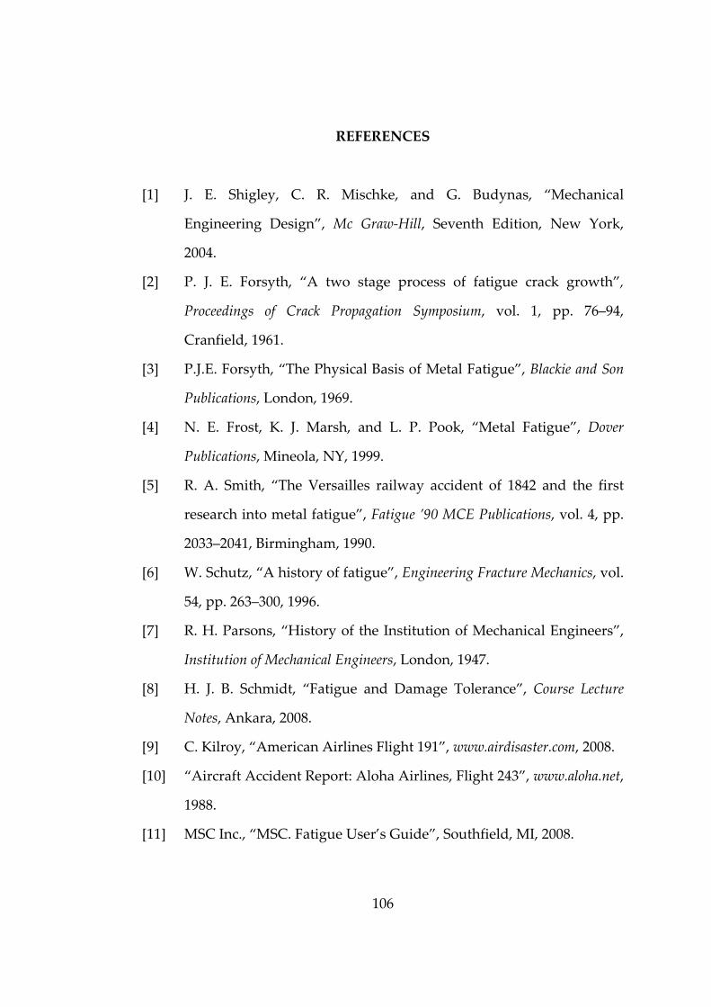
106
REFERENCES
[1] J. E. Shigley, C. R. Mischke, and G. Budynas, “Mechanical
Engineering Design”, Mc Graw‐Hill, Seventh Edition, New York,
2004.
[2] P. J. E. Forsyth, “A two stage process of fatigue crack growth”,
Proceedings of Crack Propagation Symposium, vol. 1, pp. 76–94,
Cranfield, 1961.
[3] P.J.E. Forsyth, “The Physical Basis of Metal Fatigue”, Blackie and Son
Publications, London, 1969.
[4] N. E. Frost, K. J. Marsh, and L. P. Pook, “Metal Fatigue”, Dover
Publications, Mineola, NY, 1999.
[5] R. A. Smith, “The Versailles railway accident of 1842 and the first
research into metal fatigue”, Fatigue ’90 MCE Publications, vol. 4, pp.
2033–2041, Birmingham, 1990.
[6] W. Schutz, “A history of fatigue”, Engineering Fracture Mechanics, vol.
54, pp. 263–300, 1996.
[7] R. H. Parsons, “History of the Institution of Mechanical Engineers”,
Institution of Mechanical Engineers, London, 1947.
[8] H. J. B. Schmidt, “Fatigue and Damage Tolerance”, Course Lecture
Notes, Ankara, 2008.
[9] C. Kilroy, “American Airlines Flight 191”, www.airdisaster.com, 2008.
[10] “Aircraft Accident Report: Aloha Airlines, Flight 243”, www.aloha.net,
1988.
[11] MSC Inc., “MSC. Fatigue User’s Guide”, Southfield, MI, 2008.
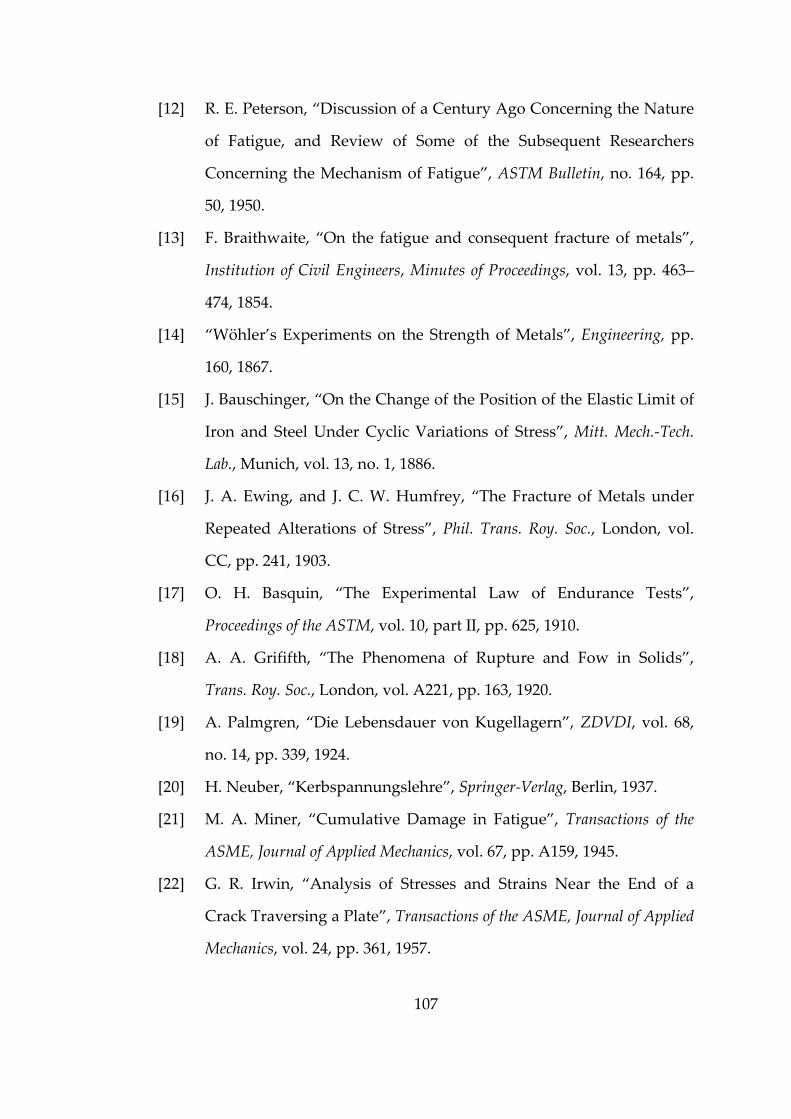
107
[12] R. E. Peterson, “Discussion of a Century Ago Concerning the Nature
of Fatigue, and Review of Some of the Subsequent Researchers
Concerning the Mechanism of Fatigue”, ASTM Bulletin, no. 164, pp.
50, 1950.
[13] F. Braithwaite, “On the fatigue and consequent fracture of metals”,
Institution of Civil Engineers, Minutes of Proceedings, vol. 13, pp. 463–
474, 1854.
[14] “Wöhler’s Experiments on the Strength of Metals”, Engineering, pp.
160, 1867.
[15] J. Bauschinger, “On the Change of the Position of the Elastic Limit of
Iron and Steel Under Cyclic Variations of Stress”, Mitt. Mech.‐Tech.
Lab., Munich, vol. 13, no. 1, 1886.
[16] J. A. Ewing, and J. C. W. Humfrey, “The Fracture of Metals under
Repeated Alterations of Stress”, Phil. Trans. Roy. Soc., London, vol.
CC, pp. 241, 1903.
[17] O. H. Basquin, “The Experimental Law of Endurance Tests”,
Proceedings of the ASTM, vol. 10, part II, pp. 625, 1910.
[18] A. A. Grififth, “The Phenomena of Rupture and Fow in Solids”,
Trans. Roy. Soc., London, vol. A221, pp. 163, 1920.
[19] A. Palmgren, “Die Lebensdauer von Kugellagern”, ZDVDI, vol. 68,
no. 14, pp. 339, 1924.
[20] H. Neuber, “Kerbspannungslehre”, Springer‐Verlag, Berlin, 1937.
[21] M. A. Miner, “Cumulative Damage in Fatigue”, Transactions of the
ASME, Journal of Applied Mechanics, vol. 67, pp. A159, 1945.
[22] G. R. Irwin, “Analysis of Stresses and Strains Near the End of a
Crack Traversing a Plate”, Transactions of the ASME, Journal of Applied
Mechanics, vol. 24, pp. 361, 1957.
108
[23] W. Weibull, “A Statistical Distribution Function of Wide
Applicability”, Journal of Applied Mechanics, pp. 293, 1951.
[24] S. S. Manson, “Discussion of Ref. [25]”, Trans. ASME, J. Basic Eng.,
vol. 84, no. 4, p. 537, 1962.
[25] J. F. Tavernelli, and L. F. Coffin, “Experimental Support for
Generalized Equation Predicting Low Cycle Fatigue”, Transactions of
the ASME, Journal of Basic Engineering, vol. 84, no. 4, pp. 533, 1962.
[26] T. H. Topper, B. I. Sandor, and J. Morrow, “Cumulative Fatigue
Damage Under Cyclic Starin Control”, Journal of Materials, vol. 4, no.
1, p. 189, 1969.
[27] M. Matsuishi, and T. Endo, “Fatigue of Metals Subjected to Varying
Stress”, Japan Society of Mechanical Engineers, Japan, 1968.
[28] W. Elber, “Fatigue Crack Closure under Cyclic Tension”,
Engineering Fracture Mechanics, vol. 2, pp. 37, 1970.
[29] P. C. Paris, “Testing for Very Slow Growth of Fatigue Cracks”, Closed
Loop, vol. 2, no. 5, 1970.
[30] S. O. Rice, “Mathematical Analysis of Random Noise”, Selected Papers
on Noise and Stochastic Processes, Dover, New York, 1954.
[31] J. S. Bendat, “Probability functions for random responses”, NASA
report on contract NAS‐5‐4590, 1964.
[32] P. H. Wirsching, M. C. Light, “Fatigue under wide band random
loading”, Journal of Structural Division, ASCE, pp. 1593‐1607, 1980.
[33] G. K. Chaudhury, and W. D. Dover, “Fatigue Analysis of Offshore
Platforms Subject to Sea Wave Loading”, International Journal of
Fatigue, vol. 7, 1985.
109
[34] J. M. Tunna, “Fatigue Life Prediction for Gaussian Random Loads at
the Design Stage”, Fatigue Fact Engineering Mat. Struct., vol. 9, no. 3,
pp. 169‐184, 1986.
[35] J. C. P. Kam, and W. D. Dover, “Fast Fatigue Assessment Procedure
for Offshore Structures under Random Stress History”, Proceedings of
the Institution of Civil Engineers, vol. 85, part 2, pp. 689‐700, 1988.
[36] D. S. Steinberg, “Vibration Analysis for Electronic Equipment”, John
Wiley & Sons, 3rd edition, USA, 2000.
[37] T. Dirlik, “Application of computers in Fatigue Analysis”, Ph.D.
Thesis, University of Warwick, 1985.
[38] W. F. Wu, H. Y. Liou, and H. C. Tse, “Estimation of fatigue damage
and fatigue life of Components under Random Loading”,
International Journal of Pressure Vessels & Piping, vol. 72, pp. 243‐249,
1997.
[39] N. Bishop, A. Caserio, and C. Mesa, “Vibration Fatigue Analysis in
the Finite Element Environment”, Americas User Conference,
California, 1998.
[40] H. Y. Liou, W. F. Wu, and C. S. Shin, “A modified model for the
estimation of fatigue life derived from random vibration theory”,
Probabilistic Engineering Mechanics, vol. 14, pp. 281‐288, 1999.
[41] X. Pitoiset, A. Preumont, and A. Kernilis, “Tools for Multiaxial
Fatigue Analysis of Structures Submitted to Random Vibrations”,
Active Structures Laboratory, Brussels, 1999.
[42] G. Petrucci, and B. Zuccarello, “On the estimation of the fatigue cycle
distribution from spectral density data”, Department of Mechanics
and Aeronautics, University of Palermo, Italy, 2004.
110
[43] G. Petrucci, and B. Zuccarello, “Fatigue Life Prediction under Wide
Band Random Loading”, Department of Mechanics and Aeronautics,
University of Palermo, Italy, 2004.
[44] X. Pitoiset, and A. Preumont, “Spectral Methods for Multi‐axial
Random Fatigue Analysis of Metallic Structures”, International
Journal of Fatigue, vol. 22, pp. 541–550, 2000.
[45] R. Tovo, “Cycle Distribution and Fatigue Damage under Broad‐band
Random Loading”, International Journal of Fatigue, vol. 24, pp. 1137–
1147, 2002.
[46] N. A. Siddiqui, and S. Ahmad, “Fatigue and fracture reliability of
TLP tethers”, Marine Structures 14, pp. 331‐352, 2001.
[47] P. L. Tu, Y. C. Chan, and J. K. L. Lai, “Effect of Inter‐metallic
Compounds on Vibration Fatigue of μBGA Solder Joint”, IEEE
Transactions on Advanced Packaging, vol.24, no.2, pp. 197‐206, 2001.
[48] D. Benasciutti, and R. Tovo, “Spectral Methods for Lifetime
Prediction under Wide‐band”, International Journal of Fatigue, vol. 27,
pp. 867–877, 2005.
[49] I. Rychlik, “On the ‘Narrow‐band’ Approximation for Expected
Fatigue Damage”, Prob. Eng. Mech., vol. 8, pp. 1‐4, 1993.
[50] H. O. Madsen, S. Krenk, and N. C. Lind, “Methods of Structural
Safety”, Englewood Cliffs: Prentice‐Hall, 1986.
[51] M. Aykan, “Vibration Fatigue Analysis of Equipments used in
Aerospace”, M.Sc. Thesis, Middle East Technical University, Ankara,
2005.
[52] N. W. M. Bishop, and F. Sherratt, “Finite Element Based Fatigue
Calculations”, NAFEMS, Germany, 2000.
111
[53] “ASTM Designation E 1049‐85: Standard Practices for Cycle
Counting in Fatigue Analysis”, ASTM, 1985.
[54] Y. Murakami, “The Rainflow Method in Fatigue”, Butterworth‐
Heinemann, Oxford.
[55] E. Kreyszig, “Advanced Engineering Mathematics”, Seventh Edition.
John Wiley & Sons, 2005.
[56] J. W. Cooley, and J. W. Tukey, “An Algorithm for the Machine
Calculation of Complex Fourier Series”, Math. Comp., vol. 19, pp.297‐
301, 1965.
[57] N. W. M. Bishop, N. Davies, A. Caserio, and S. Kerr, “Fatigue
Analysis of an F16 Navigation Pod”, www.randomvibration.com, 2000.
[58] J. C. P. Kam, and W. D. Dover, “Fast Fatigue Assessment Procedure
for Offshore Structures under Random Stress History”, Proc. Instn.
Civ. Engrs., Part 2, vol. 85, pp. 689‐700, 1988.
[59] M. M. Rahman, A. K. Ariffin, N. Jamaludin, C. H. C. Haron, and R.
A. Bakar, “Fatigue Life Prediction of Two‐Stroke Free Piston Engine
Mounting Using Frequency Response Approach”, European J. of
Scientific Research, vol. 22, pp. 480‐493, 2008.
[60] J. S. Bendat, and A. G. Piersol, “Random Data: Analysis and
Measurement Procedures”, John Wiley and Sons, NY, 1986.
[61] T. Lagoda, E. Macha, and R. Pawliczek, “The influence of the mean
stress on fatigue life of 10HNAP steel under random loading”,
International Journal of Fatigue, vol. 23, pp. 283‐291, 2000.
[62] R. Hathaway, and K. W. Long “Transducers and Acquisition Data”,
Elsevier Butterworth‐Heinemann, USA, 2005.
[63] B. Kocer, Y. Yazicioglu, S. Dag, “On the Generation of a Loading
History with Zero Mean for a Structure Subjected to Multiaxial

112
Variable Stresses”, Proceedings of The Ninth International Conference on
Multiaxial Fatigue & Fracture (ICMFF9), June 7‐10, 2010, Parma, Italy.
[64] Leissa, A. W., “Vibration of Plates”, Aeronautics and Space and
Administration, Washington, 1969.
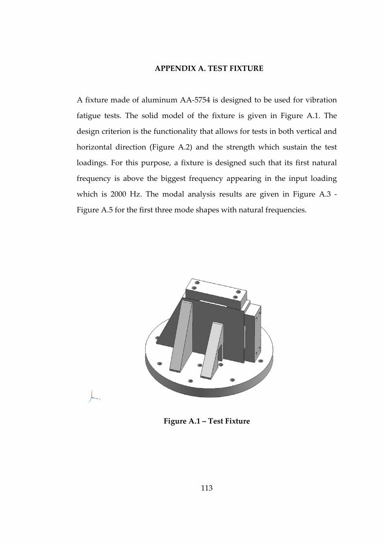
113
APPENDIX A. TEST FIXTURE
A fixture made of aluminum AA‐5754 is designed to be used for vibration
fatigue tests. The solid model of the fixture is given in Figure A.1. The
design criterion is the functionality that allows for tests in both vertical and
horizontal direction (Figure A.2) and the strength which sustain the test
loadings. For this purpose, a fixture is designed such that its first natural
frequency is above the biggest frequency appearing in the input loading
which is 2000 Hz. The modal analysis results are given in Figure A.3 ‐
Figure A.5 for the first three mode shapes with natural frequencies.
Figure A.1 – Test Fixture
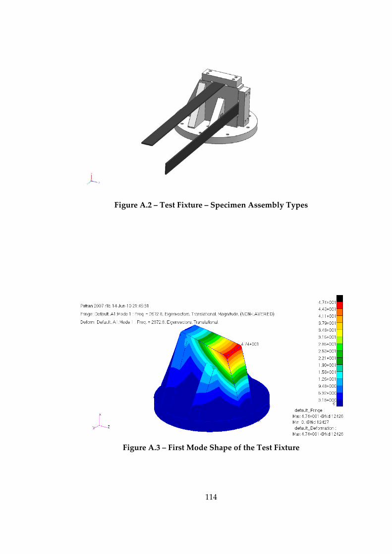
114
Figure A.2 – Test Fixture – Specimen Assembly Types
Figure A.3 – First Mode Shape of the Test Fixture
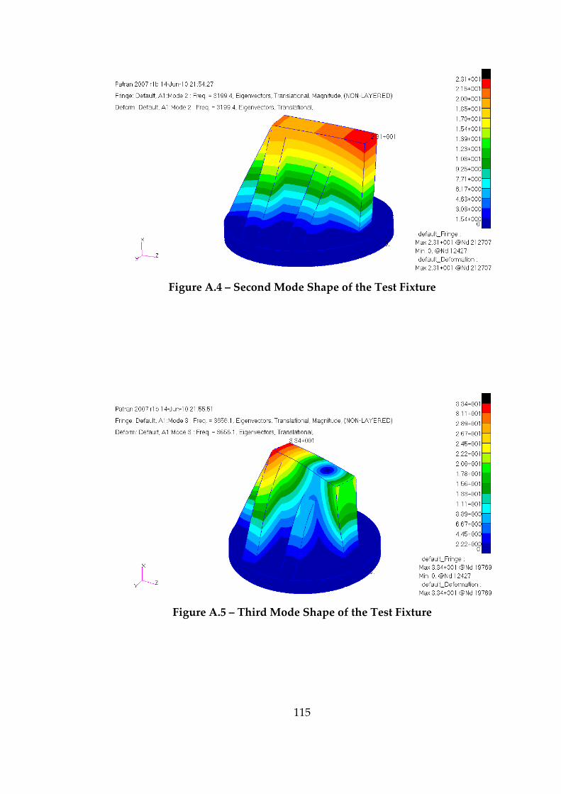
115
Figure A.4 – Second Mode Shape of the Test Fixture
Figure A.5 – Third Mode Shape of the Test Fixture
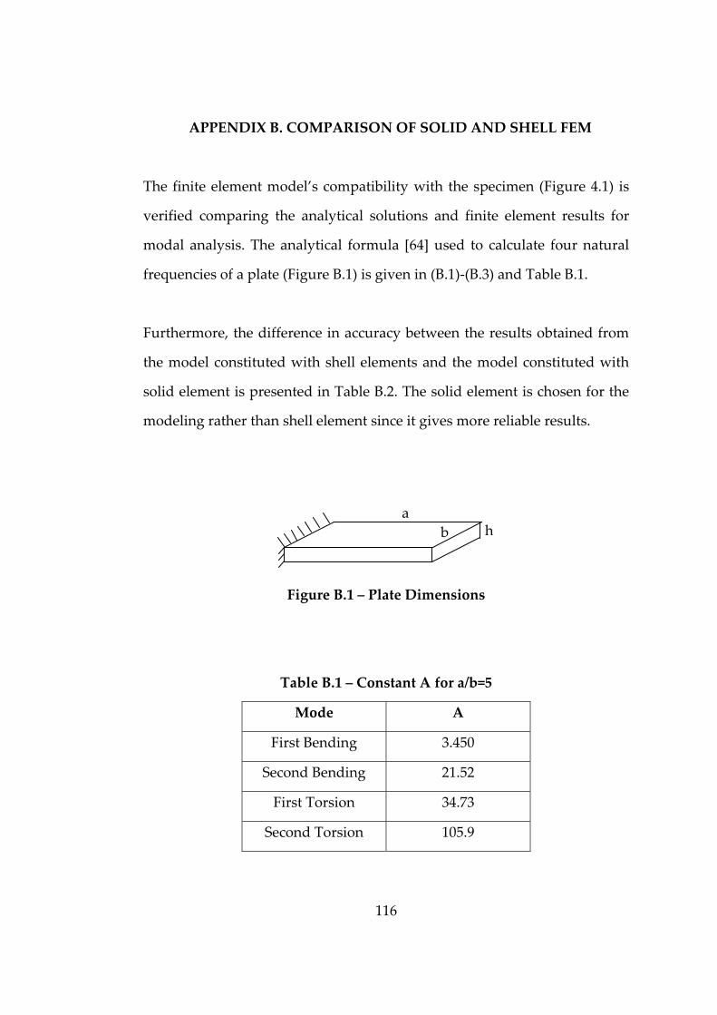
116
APPENDIX B. COMPARISON OF SOLID AND SHELL FEM
The finite element model’s compatibility with the specimen (Figure 4.1) is
verified comparing the analytical solutions and finite element results for
modal analysis. The analytical formula [64] used to calculate four natural
frequencies of a plate (Figure B.1) is given in (B.1)‐(B.3) and Table B.1.
Furthermore, the difference in accuracy between the results obtained from
the model constituted with shell elements and the model constituted with
solid element is presented in Table B.2. The solid element is chosen for the
modeling rather than shell element since it gives more reliable results.
Figure B.1 – Plate Dimensions
Table B.1 – Constant A for a/b=5
Mode A
First Bending 3.450
Second Bending 21.52
First Torsion 34.73
Second Torsion 105.9
b h a
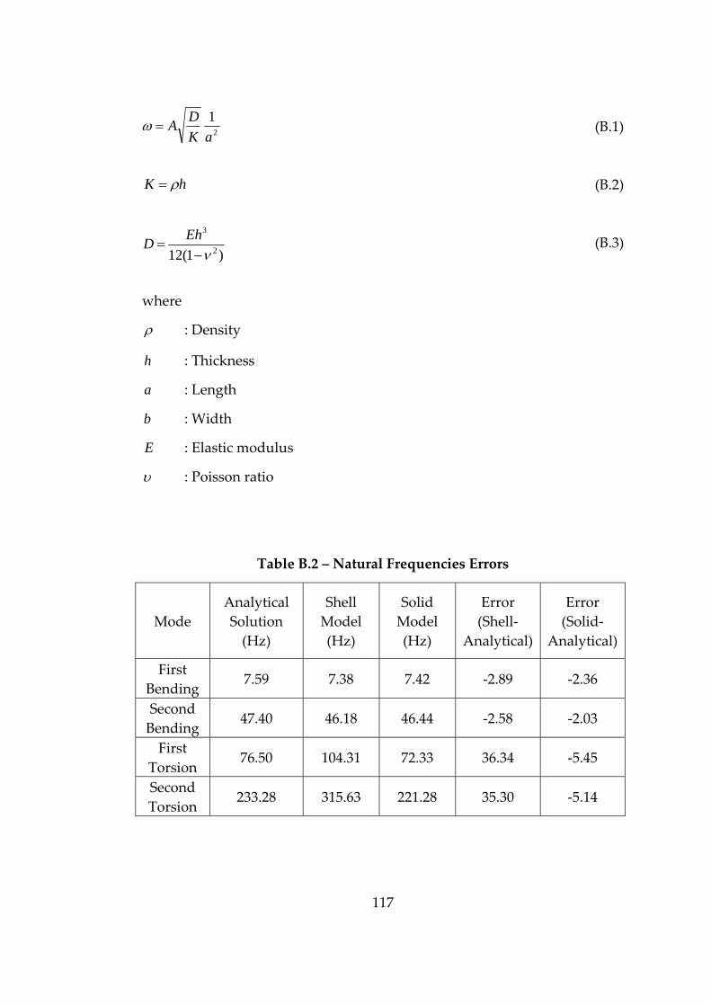
117
(B.1)
(B.2)
(B.3)
where
ρ : Density
h : Thickness
a : Length
b : Width
E : Elastic modulus
υ : Poisson ratio
Table B.2 – Natural Frequencies Errors
Mode Analytical Solution (Hz)
Shell Model (Hz)
Solid Model (Hz)
Error (Shell‐
Analytical)
Error (Solid‐
Analytical)
First Bending
7.59 7.38 7.42 ‐2.89 ‐2.36
Second Bending
47.40 46.18 46.44 ‐2.58 ‐2.03
First Torsion
76.50 104.31 72.33 36.34 ‐5.45
Second Torsion
233.28 315.63 221.28 35.30 ‐5.14
2
1aK
DA=ω
hK ρ=
)1(12 2
3
ν−=
EhD


![Statics and Dynamics of Super Elliptical Homogeous and FGM Plates [Homojen Ve FGM Süper Eliptik Plakların Statik Ve Dinamiği]](https://static.fdocuments.in/doc/165x107/55cf96d2550346d0338dff00/statics-and-dynamics-of-super-elliptical-homogeous-and-fgm-plates-homojen.jpg)