Vibration fatigue and simulation of damage on shaker table ... · 5th Fatigue Design Conference,...

Available online at www.sciencedirect.com

Procedia Engineering 00 (2013) 000–000

www.elsevier.com/locate/procedia

1877-7058 © 2013 The Authors. Published by Elsevier Ltd. Selection and peer-review under responsibility of CETIM, Direction de l'Agence de Programme.

5th Fatigue Design Conference, Fatigue Design 2013

Vibration fatigue and simulation of damage on shaker table tests: the influence of clipping the random drive signal

Frédéric Kihma*, David Delauxb aHBM-nCode Products Division, Technology Center, Brunel Way, Catcliffe, Rotherham, S60 5WG, UK

bValeo, 43 Rue Bayen, 75848 Paris, France

Abstract

Suppliers of shaker controllers often use a technique called ‘sigma clipping’ to prevent the amplifier from encountering too high amplitude peaks. Sigma clipping is most commonly used to make sure a shaker system will be sufficiently powerful to reproduce the required random spectrum. The level of clipping is measured via the crest factor, which is expressed as a ratio between the absolute maximum of the signal and its root-mean-square (RMS) value. Such clipped drive signals are therefore no longer Gaussian, since their probability distribution functions (PDF) are truncated at high values. The clipped drive signal is then amplified and filtered by a system made up of the shaker itself followed by the unit under test. Although the local stress and strain responses do not show any obvious clipping, their statistics may be affected. This can feed through to fatigue damage, which is known to be exponentially related to strain amplitudes. A legitimate question is therefore “how does clipping affect damage?” This paper studies and quantifies the influence of clipping experimentally, numerically and theoretically. There are many objectives and underlying questions to consider. For the test technicians, what level of clipping to choose in order to represent the damage due a Gaussian environment? Whereas for the simulation engineers, how to enhance damage estimations by taking into account the level of clipping? © 2013 The Authors. Published by Elsevier Ltd. Selection and peer-review under responsibility of CETIM, Direction de l'Agence de Programme.

"Keywords: Fatigue; crest factor; Sigma clipping; random shaker tests, gaussian, statistics"

* Corresponding author. Tel.: +33 130182020; fax: +33 130182019.

E-mail address: [email protected]

2 Kihm F./ Procedia Engineering 00 (2013) 000–000

1. Introduction

When performing random vibration tests, it is common to expect a Gaussian distribution of both the input acceleration and the responses.

However in practice, the controller typically clips the drive signal to prevent too high amplitude peaks. It therefore allows the shaker system to deliver more power, because it can represent random signals of greater RMS power by clipping the rare high amplitude peaks. The high amplitudes are truncated above a given level and the resulting clipped signal is no longer Gaussian. So, the crucial question is: “What is the influence of clipping the drive signal on the fatigue life of a specimen during a random shaker test?”.

Some tests were performed on a specimen, instrumented with an accelerometer and strain gages. The drive signal was clipped at various levels. The time domain signals of the drive and the responses were recorded.

This paper will study the clipping of the drive signal and the characteristics of the responses using frequency analysis, statistical analysis and rainflow cycle counting. The results are compared with those obtained from unclipped input signals and with theory.

Nomenclature

FFT Fast Fourier Transform DFT Discrete Fourier Transform FRF Frequency Response Function IRF Impulse Response Function RMS Root Mean Square CF Crest Factor PDF Probability Density Function i.i.d. Independently and identically distributed ln() Natural logarithm (to the base e) σ Standard deviation µ Mean Ep Expectation of the number of peaks per seconds T Exposure duration κx Kurtosis value of random variable X mxn nth order moment of random variable X cxn nth order cumulant of random variable X

Kihm F./ Procedia Engineering 00 (2013) 000–000 3

2. Clipping the drive signal

2.1. Statistics for an ideal Gaussian stationary random signal

A random variable x is said to be Gaussian if its probability density function (PDF) is given by:

( )2

222

1( )

2

x

XP x e

µσ

πσ

−−

= (1)

Where µ is the mean and σ is the standard deviation. Note that in the case of a centered process, standard deviation is equal to RMS.

The standardized statistical moments for a centered Gaussian PDF are given in table 1.

Table 1. Statistics linked with Gaussian distributions

Standardized moment Name Value for a Gaussian process

1 mean µ

2 variance σ²

3 skewness 0

4 kurtosis 3

From the PDF, it is easy to calculate what portion of the signal will exceed a given level. Table 2 illustrates what percentage of the data will lie between +/- multiples of the RMS value.

Table 2. Statistics linked with Gaussian distributions

Crest Factor N % data within +/- N*RMS

2 95.45

3 99.73

4 99.99

5 99.999943

6 99.9999998027

Formulations exist for finding the maximum value for a band-limited Gaussian process within a period of time [1]

such that one can find the maximum value a signal is likely to experience for a given duration. For instance, when considering the excitation spectrum used in this paper and displayed in figure 3, the necessary exposure duration to reach a maximum of 6*RMS is a bit over 270 hours! This means that during a few hours of exposure, there is no need to set sigma clipping over 6.0 since the signal is extremely unlikely to reach this level. However, with sigma clipping of 3.0, a common default, this would clip less than 0.3% of the signal. In the present case, the level 3*RMS is crossed once per second, which questions whether 3.0 is a valid default value.

2.2. Abrupt clipping

Abrupt clipping is a technique that simply cuts off the peaks at a given level. The resulting signal is therefore non-Gaussian. Abrupt clipping directly influences the crest factor (CF) of the resulting signal. The crest factor of a signal is defined as the maximum value divided by the RMS of the signal.

Although very easy to implement - either by analogue or digital ways - abrupt clipping introduces strong high frequency distortion in the resulting spectrum [2].

Conceptually, this can be understood by thinking of clipping a sine wave, where the spectrum of a sine wave is a single line at the fundamental frequency. The more the sine wave is clipped, the closer it gets to a square wave. The Fourier series of a square wave is made up of one line at the fundamental frequency and an infinite number of odd harmonics, whose amplitudes decrease as 1/f.


2.3. Soft clipping

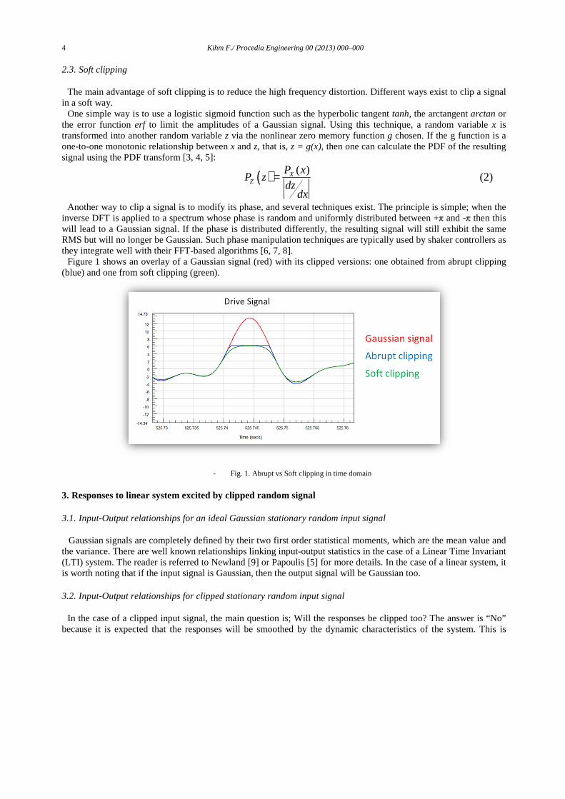
The main advantage of soft clipping is to reduce the high frequency distortion. Different ways exist to clip a signal in a soft way.

One simple way is to use a logistic sigmoid function such as the hyperbolic tangent tanh, the arctangent arctan or the error function erf to limit the amplitudes of a Gaussian signal. Using this technique, a random variable x is transformed into another random variable z via the nonlinear zero memory function g chosen. If the g function is a one-to-one monotonic relationship between x and z, that is, z = g(x), then one can calculate the PDF of the resulting signal using the PDF transform [3, 4, 5]:

( ) ( )XZ

P xP z

dzdx

= (2)

Another way to clip a signal is to modify its phase, and several techniques exist. The principle is simple; when the inverse DFT is applied to a spectrum whose phase is random and uniformly distributed between +π and -π then this will lead to a Gaussian signal. If the phase is distributed differently, the resulting signal will still exhibit the same RMS but will no longer be Gaussian. Such phase manipulation techniques are typically used by shaker controllers as they integrate well with their FFT-based algorithms [6, 7, 8].

Figure 1 shows an overlay of a Gaussian signal (red) with its clipped versions: one obtained from abrupt clipping (blue) and one from soft clipping (green).

- Fig. 1. Abrupt vs Soft clipping in time domain

3. Responses to linear system excited by clipped random signal

3.1. Input-Output relationships for an ideal Gaussian stationary random input signal

Gaussian signals are completely defined by their two first order statistical moments, which are the mean value and the variance. There are well known relationships linking input-output statistics in the case of a Linear Time Invariant (LTI) system. The reader is referred to Newland [9] or Papoulis [5] for more details. In the case of a linear system, it is worth noting that if the input signal is Gaussian, then the output signal will be Gaussian too.

3.2. Input-Output relationships for clipped stationary random input signal

In the case of a clipped input signal, the main question is; Will the responses be clipped too? The answer is “No” because it is expected that the responses will be smoothed by the dynamic characteristics of the system. This is


verified by the results of the test (see figure 11 in section 5.3) and a simple explanation is given here. Consider a single degree of freedom system as shown in Figure 2. If the input load is a sine wave, the expected

response is a sine wave with a given lag and amplitude. If a cycle is clipped just like that shown in Figure 2, it is expected that the response is similar as one obtained from a full regular cycle. This behavior is due to the inertia of the system because the system is responding dynamically (with some memory) and not statically (as if it was made only of a spring). The future position of the system is dependent upon the past positions and its dynamic characteristics. So even though the input sine wave is clipped at some instant in time, the response will continue to oscillate.

- Fig. 2. SDOF system with input/output relationships

The fact that a signal is clipped (whether abruptly of softly) is noticeable in the “queues” of the PDF. The “queues” of a distribution are described by the higher order, even numbered, statistical moments. For example, the 4th statistical moment, referred to as the kurtosis is a known measure of tails thickness. Some example PDFs of clipped signals are shown in figure 8.

Cumulants are an alternative to the statistical moments. When dealing with higher order statistics, cumulants are often preferred to moments because of their interesting properties [10] such as additivity and homogeneity. This means that the cumulants of the weighted sum of n independent random variables are the weighted sum of the cumulants of each random variable. A corollary to this is that cumulants are additive under convolution.

For a zero-mean, symmetric PDF, only the even orders need to be considered. It is often convenient to consider up to order 4 only, because higher orders or cumulants are difficult to estimate and generally show higher sampling variability. Also, higher order moments or cumulants have a very subtle effect, seen in some specific aspect of the PDF shape.

The 2nd and 4th cumulants of the response signal cy2 and cy4 can be derived from the 2nd and 4th cumulants cx2 and cx4 of an independent and identically distributed (i.i.d) input signal and from the coefficients hi of the impulse response function as:

2

2 2

44 4

y x i

y x i

c c h

c c h

=

=∑

∑ (3)

The relationship between cumulants and moments are given by the Leonov and Shiryayev formulae [10] for the 2nd and 4th order cumulants cy2 and cy4 as a function of the 2nd and 4th order moments my2 and my4. In the case of a zero-mean signal, these are:

2 2

4 4 2

3 ²y y

y y y

c m

c m m

=

= − (4)

The output kurtosis is obtained by using equations (4) with the definition of the kurtosis giving:

4 4

2 22 2

3.0y yy

y y

m c

m cκ = = + (5)

The output kurtosis of a zero-mean process expressed in terms of the impulse response and input kurtosis is


obtained by substituting equations (3) into equation (5) giving

( )

( )4

223.0 3.0i

y x

i

h

hκ κ= − +∑

∑ (6)

Note that the value of the output kurtosis is between the value of the input kurtosis and 3.0. In relation to equation (6), an IRF with long decaying oscillations will maximize the squared terms in the

denominator compared to the terms raised to the 4th power in the numerator. This will lead to a lower output kurtosis for a lightly damped system than for a more heavily damped one. This behavior is consistent with the observation that the output kurtosis tends to Gaussian as the bandwidth of the filter, i.e, the amount of damping, decreases [11, 12]. A similar equation can be derived for the higher order statistical moments. As the order increase, higher order statistics converge even quicker to the values corresponding to a Gaussian distribution, since the exponents increase. Also, the convergence is further accelerated in the case of narrow band processes.

Equation (6) is only valid for i.i.d. processes which have no temporal dependency and are spectrally flat (i.e. white noise). Equation (6) can be generalized to non-spectrally flat (i.e. colored) noise by considering the colored noise as a filtered version of spectrally flat noise, that is,

( )

( ) ( )224

2 423.0 3.0

iiy x

ii

cf

cfκ κ= − +∑∑

∑∑ (7)

where ci are the values of the autocorrelation function of the input noise and fi are the values of the convolution of the autocorrelation function with the IRF.

3.3. Some preliminary conclusions

Sigma clipping introduces high frequency distortion in the spectrum and cuts off the tails of the PDF, characterized by the kurtosis. When the clipped signal is used as an excitation, the responses to a linear system tend towards a normal (i.e. Gaussian) distribution. Depending on the bandwidth of the system, the value of the output kurtosis lies between the value of the input kurtosis and 3.0. A relationship linking input and output kurtosis has been described. This relationship depends on the characteristics of the linear time invariant system and the autocorrelation function of the input signal.

4. The experiment

4.1. The test article

Some shaker tests were performed at Valeo, La Verrière Research Center. The test specimen was a passenger’s car radiator for the European market. The radiator was solidly clamped on the shaker, using a rigid structure (no rubbers interface between frame and radiator). A view of the test rig and test article is shown in figure 3.


- Fig. 3. Radiator under test

4.2. Data collection

Strain gages were positioned close to the traditional hot spots: at the connections between the tubes and the header, see figure 4. This location is a probable failure zone. Accelerometers were positioned to capture the control signal and some responses on the top and on the header of the radiator.

- Fig. 4. Strain gage at the connection between a tube and the header

Data acquisition was performed at 4096 samples per second giving an excellent resolution of over 40 points per cycle at the highest frequency considered.

4.3. Tests

Random tests were based on a typical acceleration PSD of 1.77 gRMS, illustrated figure 5 below. Such a PSD was synthesized from Road Load Data using the classical “Accelerated Testing” (also known as “Test Tailoring”) approach [13, 14]. This specification is applied for 30 hours in order to cover the reliability targets of the carmaker.


- Fig. 5. Excitation PSD used

Several random tests of 15 minutes each were performed. A different value of abrupt sigma clipping was used for each, ranking from 2 to 5.

5. Results obtained

All results presented below were made after some preliminary checks: linearity was ensured by increasing the RMS level from 0.5 gRMS to 1 gRMS and finally to 1.77 gRMS. Also, the signals were checked against outliers, drifts, etc.

Note that, although only one strain gage positioned close to the tube-header junction is mentioned here, similar results were obtained with the other strain gages. In this paper, the authors decided to concentrate on one result for the sake of simplicity.

5.1. Dynamics of the test article

Figure 6 shows the frequency response function (FRF) linking input acceleration and strain response, obtained with the default sigma clipping of 3.0. This FRF will be called the “strain-g” FRF.

- Fig. 6. Strain-based FRF


This and the other strain gages show a similar behavior; showing several resonances in the frequency range of the loading.

5.2. Loading signals

Figure 7 compares the drive signals obtained for sigma clipping (SC=) 2, 3 and 5. The dashed black line represents 3 standard deviations (+3 sigma) or -3 standard deviations (-3 sigma) of the signal.

- Fig. 7. Time domain representation of the drive signals

Probability distribution functions (PDF) were calculated from the control signals obtained with SC=2, 3 and 5 and are displayed in figure 8. Since much of the difference in the distributions is in the “tails”, it easier to compare the PDF plots with the vertical axis plotted using a logarithmic scale, as shown in Figure 8.

The black dashed line shows an ideal Gaussian distribution with theoretically infinite CF as the tails go to infinity. Including the Gaussian distribution helps to demonstrate how the clipped signals deviate from it. It is clear that the PDF of the signal associated with SC=5 is the closest to the Gaussian distribution.


- Fig. 8. PDF of the drive signals

From the PDFs, one can derive the non-linear relationship between the Gaussian signal and its clipped version, based on the PDF transform mentioned in section 2. This non-linear relationship is displayed in figure 9 for the cases where SC=2 and 3. The black dashed line represents the identity (linear) law and helps to demonstrate how the non-linear relationships deviate from it. Here it becomes clear that the transition between unchanged and sigma clipped levels is continuous and not completely abrupt, like an instantaneous step change.

- Fig. 9. Input-output relationship in case of clipping

Figure 10 shows the Power Spectral Densities (PSD) calculated from the drive signals obtained for SC=2, 3 and 5. As expected by the theory [2], clipping introduces higher energies in the out-of-band frequencies. Figure 10 also shows that decreasing the value of sigma clipping introduces more distortion and therefore reduces the dynamic range. The contrary applies too i.e. increasing the default clipping to 6 for instance would even further increase the dynamic range.


- Fig. 10. High frequency distortion due to clipping

Table 3 shows some basic statistics extracted from the drive signals obtained for SC=2, 3, 5 and from an ideal Gaussian signal of same RMS.

Table 3. statistics of the drive signals.

Signal Mean RMS Crest Factor Skewness Kurtosis

Sigma clipping 2 0 1.76 2.2 0 2.4

Sigma clipping 3 0 1.77 3.1 0 2.9

Sigma clipping 5 0 1.77 4.8 0 3.0

ideal Gaussian 0 1.77 4.8 0 3.0

The actual crest factor is a bit higher than the user-defined sigma clipping value. The kurtosis values decrease

when sigma clipping is low. This is in accordance with the expectation since the signal spends less time at the extreme values.

5.3. Influence of clipping on the responses

The signals collected from the sensors on the test article represent the responses to the clipped input. The responses are a filtered version of the input and are a result of the dynamics of the test article. Thus the responses may not have the same characteristics as the input. The objective of this section is to evaluate the impact of sigma clipping on the responses.

The time domain responses collected on a single strain gage have been converted to stress using a linear scale factor and are presented in Figure 11. The same convention is used as in figure 7, i.e. the dashed black lines correspond to the +/- 3 Sigma levels.

PS

D


- Fig. 11. Stress responses at strain gage

The +/- 3 sigma level are exceeded in all cases, even with the low sigma clipping of 2 applied to the input. The time responses extracted from the accelerometers show the same behavior. The clipping of the input is not identically reproduced by the responses.

Table 4 shows the basic statistics for the response strain gauge:

Table 4. Statistics of the response strain signals.

Signal Mean RMS Crest Factor Skewness Kurtosis

Sigma clipping 2 0 15.69 4.61 0 2.93

Sigma clipping 3 0 15.71 4.63 0 2.98

Sigma clipping 5 0 15.75 4.91 0 3.0

ideal Gaussian 0 15.78 4.91 0 3.0

Again, it is clear that sigma clipping applied on the input is not identically reproduced on the output signals.

Probability distribution functions (PDF) were calculated from the responses obtained from the various control signals obtained with CF=2, 3 and 5 and are all very similar. The responses therefore tend to be Gaussian.

Applying equation 7 gives excellent correlation for the output kurtosis values: 2.96 for SC= 2 and 2.99 for SC=3 and 3.0 for the higher values of sigma clipping.

5.4. Influence of clipping on the fatigue life

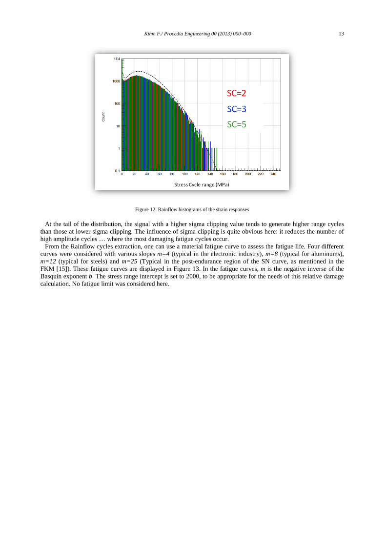
The fatigue life of a component is primarily dependent on the strain amplitude response at critical failure locations. The Rainflow cycle counting algorithm enables a time varying stress or strain to be reduced into its fatigue cycles, where each cycle has a range and a mean. A first approach to fatigue is to compare the cycles extracted from signals when various sigma clipping were applied. Figure 12 shows the Rainflow histograms obtained for the 3 values of sigma clipping used.


Figure 12: Rainflow histograms of the strain responses

At the tail of the distribution, the signal with a higher sigma clipping value tends to generate higher range cycles than those at lower sigma clipping. The influence of sigma clipping is quite obvious here: it reduces the number of high amplitude cycles … where the most damaging fatigue cycles occur.

From the Rainflow cycles extraction, one can use a material fatigue curve to assess the fatigue life. Four different curves were considered with various slopes m=4 (typical in the electronic industry), m=8 (typical for aluminums), m=12 (typical for steels) and m=25 (Typical in the post-endurance region of the SN curve, as mentioned in the FKM [15]). These fatigue curves are displayed in Figure 13. In the fatigue curves, m is the negative inverse of the Basquin exponent b. The stress range intercept is set to 2000, to be appropriate for the needs of this relative damage calculation. No fatigue limit was considered here.


Figure 13: Fatigue curves used

A low value for m results in a very steep fatigue curve, giving more importance to cycles with small amplitudes. On the contrary, a high value for the slope m results in a more horizontal fatigue curve, giving virtually no influence to cycles with small amplitudes. In this case, the fatigue damage is almost fully driven by a small number of high amplitude cycles.

Table 5 gathers the fatigue damage results obtained for the various materials and sigma clipping used. An ideal Gaussian (i.e. no clipping) loading was created and its damage also calculated. The damage values are scaled and displayed as a percentage of the damage calculated for the ideal Gaussian case.

Table 5. Damage values.

Signal Damage with m=4

Electronics

Damage with m=8

Aluminum

Damage with m=12

Steel

Damage with m=25

FKM

Sigma clipping 2 93% 84% 71% 24%



ideal Gaussian 100% 100% 100% 100%

Clearly, a low sigma clipping value will penalize damage and this is more pronounced when the slope m is high.

This is as expected since sigma clipping has most effect on the high amplitude cycles. If the PDF is reduced at the tails, then it needs to be increased in other regions to get the total area under the PDF to 1.0. From a fatigue perspective, material curves with low values of m are more sensitive to these additional lower sigma peaks.

Applying sigma clipping less than 3 will lead to a less damaging test than expected from a truly Gaussian load (where no clipping occurs) - and this is true regardless of the material used.

The state of the art in reliability testing is a fatigue computation of the specification based on road load data at iso-damage. In the automotive domain, a test accelerated in 30 hours per axis with a sigma clipping of 3 is considered as representative of the vehicle risks. Valeo experience has proved this fact.


In table 6, damage values are now scaled with respect to the damage calculated for the typical default value of sigma clipping = 3.0. The original test duration associated with a sigma clipping of 3.0 is recalled and the equivalent test duration in the case of a sigma clipping of 5.0 is computed and displayed.

Table 6. Damage values scaled with respect to the damage of SC3 and associated test durations.

Signal Damage with m=4

Electronics

Damage with m=8

Aluminum

Damage with m=12

Steel

Damage with m=25

FKM


Sigma clipping 3 100% 100% 100% 100%

test duration with Sigma clipping 3 30 hours 30 hours 30 hours 30 hours

Sigma clipping 5 ~100 % ~100 % 104% 179%

Equivalent test duration with Sigma clipping 5 30 hours 30 hours 28.5 hours 16.8 hours

Here it becomes clear that if the industry standard was to use the default sigma clipping of 3.0, setting it to a

higher level allows reducing the test duration. For example, in the case of m=25, setting sigma clipping from 3 to 5 could potentially lead to a test reduction factor of almost 50%.

6. Conclusions

Random vibration tests with various values for sigma clipping were made on a test article instrumented with strain gages. Although this paper was produced from this particular test case, it gives an insight into the influence of sigma clipping and identifies some conclusions and recommendations.

Keeping or even reducing the value of sigma clipping below 3 seems acceptable for modal-type applications as the frequency response function seems mostly unaffected.

For endurance tests however, the user should avoid sigma clipping below 3 for several reasons. Firstly, clipping the signal introduces high frequency distortion. All the extra energy above the required cut-off frequency can cause damage to components that are sensitive to the additional higher frequency excitation and this may not be representative of the real-world excitation. This extra energy above the required cut-off frequency reduces the dynamic range. Arguably, the clipped excitation signal is no longer "random" since the high frequency distortion is highly correlated with their low frequency fundamentals.

Secondly, it noticeably reduces the fatigue damage potential on the test article, due to the reduced number of stress cycles of high amplitudes.

Thirdly, it may also lead to a reduction of energy in the specification bandwidth that further reduces the fatigue damage potential on the test article.

Considering a wider range of test articles, the default sigma clipping value of 3 may sufficiently represent the damage potential of a truly Gaussian process for:

- Electronic components - Mechanical components with fasteners such as welds - Components, where failure occurs in a material with a low fatigue slope m, such as aluminum or titanium

alloys. But if the failure is expected to occur in a material with a high fatigue slope m such as steels, irons, magnesium

alloys, etc., it is suggested to increase the sigma clipping value as much as possible to best maintain the smaller number of high amplitude cycles that are most fatigue damaging.

Finally, if the industry standard is to run tests with sigma clipping of 3, using a higher value for sigma clipping allows producing the same damage in less time. The test duration can be reduced noticeably depending on the material used and the dynamic characteristics of the system.


Acknowledgements

Special thanks to Marco Bencivenga, Dr. Arnaud Maire and Marco Bonato from Valeo for their help in setting up the test and instrumentation.

The authors are also very thankful to Dr. Karl Sweitzer for sharing his valuable experience. Thanks are also due to Rob J. Plaskitt and Dr. Andrew Halfpenny from HBM nCode for their useful comments.

References

[1] AJ Adams, NDP Barltrop "Dynamics of fixed marine structures", Butterworth Heinemann, ISBN 0 7506-1046-8 [2] Van Vleck, J. H., & Middleton, D. (1966). “The spectrum of clipped noise”. Proceedings of the IEEE, 54(1), 2-19. [3] Sweitzer, K.A., "Random vibration response statistics for fatigue analysis of nonlinear structures," Ph.D. Dissertation, Institute of Sound and

Vibration Research, University of Southampton, UK, 2006. [4] Bendat, J.S. and Piersol, A.G., Random data: Analysis and measurement procedures, Wiley-Interscience, 1971. [5] Papoulis, A., Probability, random variables, and stochastic processes (3rd edition), McGraw-Hill, Inc., 1991. [6] Steinwolf, A., "Two methods for random shaker testing with low kurtosis," in Sound & Vibration, October 2008, pp. 18-22. [7] Steinwolf, A. "Shaker random testing with low kurtosis: Review of the methods and application for sigma limiting". Shock and Vibration,

2010, 17(3), 219-231. [8] Van der Auderaa, E., Schoukens, J. and Renneboog, J., Peak Factor Minimization Using a Time-Frequency Domain Swapping Algorithm,

IEEE Transactions on Instrumentation and Measurement, Vol. 37, pp. 145-147, 1988. [9] Newland DE. (1984). “An introduction to random vibrations and spectral analysis (2nd edition) “, Longman Inc., New York. [10] Lacoume, J.-L., Amblard, P.-O., and Comon, P., Statistiques d’ordre supérieur pour le traitement du signal, Masson, 1997. [11] Rizzi, S.A., Przekop, A., and Turner, T.L., "On the response of a nonlinear structure to high kurtosis non-Gaussian random loadings,"

EURODYN 2011, 8th International Conference on Structural Dynamics, Paper 41, Leuven, Belgium, July 4-6, 2011. [12] Papoulis, A., "Narrow-band systems and Gaussianity," IEEE Transactions on Information Theory, Vol. 18, No. 1, pp. 20-27, 1972. [13] Lalanne, C. Mechanical Vibration & Shock, volume 5. London : Hermes Penton Ltd., 2002. [14] Halfpenny, A., Kihm, F. “Mission Profiling and Test Synthesis Based on Fatigue Damage Spectrum”, Proceedings of the 9th International

Fatigue Congress, Atlanta, USA, (2006). [15] FKM Analytical strength assessment – VDMA Verlag “Rechnerischer Festigkeitsnachweis für Maschinenbauteile”– 5th, revised edition,

2003.

Vibration fatigue and simulation of damage on shaker table ... · 5th Fatigue Design Conference,...

Documents

Transcript of Vibration fatigue and simulation of damage on shaker table ... · 5th Fatigue Design Conference,...