Vibration characterisation of low frequency engine...

Department of Civil and Environmental Engineering Division of Applied Acoustics Vibroacoustics Research Group CHALMERS UNIVERSITY OF TECHNOLOGY Gothenburg, Sweden 2016 Master’s Thesis 2016:5

Vibration characterisation of low frequency engine idle vibrations Master’s Thesis in the Master’s Programme Sound and Vibration ROBERT LARSSON

MASTER OF SCIENCE THESIS 2016:5

Vibration characterisation of low frequency engine idle vibrations

Master of Science Thesis in the Master’s Programme Sound and Vibration

ROBERT LARSSON

Department of Civil and Environmental EngineeringDivision of Applied AcousticsVibroacoustic research group

CHALMERS UNIVERSITY OF TECHNOLOGY

Gothenburg, Sweden 2016

Vibration characterisation of low frequency engine idle vibrationsMaster of Science Thesis in the Master’s Programme Sound and VibrationROBERT LARSSON

c� ROBERT LARSSON, 2016

Examensarbete 2016:5/ Institutionen for bygg- och miljoteknik,Chalmers tekniska hogskola 2016

Department of Civil and Environmental EngineeringDivision of Applied AcousticsVibroacoustic research groupChalmers University of TechnologySE-412 96 GothenburgSwedenTelephone: +46 (0)31-772 1000

Cover:Experimental modal analysis, mode no. 3, 6.9 Hz

Chalmers ReproserviceGothenburg, Sweden 2016

Vibration characterisation of low frequency engine idle vibrationsMaster of Science Thesis in the Master’s Programme Sound and VibrationROBERT LARSSONDepartment of Civil and Environmental EngineeringDivision of Applied AcousticsVibroacoustic research groupChalmers University of Technology

Abstract

To deliver a product with high quality impression and a comfortable ride, the vibrations in atruck seat has to be well controlled and cannot disturb the driver. In order to characterise this,modal measurements and simulations are correlated with operational data. This thesis focuseson the low frequency engine idle vibrations, 0 to 20 Hz, and its behaviour in the driver seat,with emphasis on beating phenomenon occurring at engine idle rpm.

The operational measurements use the engine as the driving source and the truck placed on aconcrete floor, which gives the correct boundary conditions for the beating phenomenon. Inthe modal measurements the truck’s front left wheel is standing on a large hydraulic shakerto excite the complete truck. A setup of measurement positions is arranged to cover all vitalparts of the truck. In order to make the results comparable the arrangement of measurementpositions is identical for both measurement methods. The advantage of having both theoperational behaviour alongside with the modal is that the driven behaviour, due to the engineexcitation, can be separated from the pure modal behaviour.

A beating phenomenon could be found in the seat base of the driver seat and with the resultsfrom both the operational and modal measurement, a mode map of the complete truck wasassembled. Two modulation frequencies were found and the measurements showed that thefirst engine order is very prominent and also di�cult to attenuate along the transfer paths fromengine to driver seat. The mode map consisted of several of the rigid body modes belongingto the engine and cab, as expected due to the low frequency range. Flexural modes in thechassis were also found. Comparing the mode map and the two modulation frequencies reviledthat ten mode types can influence the beating phenomenon and out of those five match themodulation frequencies exact.

Keywords:Vibration characterisation, Beating, Operational deflection shapes, Operational modal analysis,Modal analysis, Complete truck

i

Acknowledgements

The Master thesis project was performed at the noise and vibration laboratory at Volvo GroupTrucks Technology in Gothenburg during 2015. I want to thank everyone at the departmentfor their encouragement and positive attitude. It has been a very educative journey and now Iposses many vital learnings for the future, which I am grateful for. I would also like to thankAnders Lindstrom for the help with FE-simulations and Magnus Ahlstedt for lending me andmanoeuvring the road simulator rig.

Special thanks go to my supervisors Torbjorn Agren and Patrik Hostmad. Thank you for yoursupport and guidance through this year. I have really enjoyed our easy going and educatingdiscussions.

Last but not least I want to thank my family and especially my girlfriend for your support, itwould not have been possible to achieve this without your help.

ii

Nomenclature

Transmissibility Response vs. Response (acceleration/acceleration)

Abbreviations

A-D Analogue-DigitalBS British StandardDOF Degrees Of FreedomEO Engine OrderEMA Experimental Modal AnalysisFE-model Finite Element ModelFRF Frequency Response FunctionISO International Standardization OrganizationMIMO Multiple Input Multiple OutputNTF Noise Transfer FunctionNVH Noise, Vibration and HarshnessODS Operating Deflection ShapesOMA Operating Modal AnalysisOTPA Operating Transfer Path AnalysisRBM Rigid Body Moderpm Revolutions Per MinuteSDOF Single Degree Of FreedomSIMO Single Input Multiple OutputVTF Vibration Transfer FunctionWBV Whole Body Vibrations

iii

Contents

Abstract i

Acknowledgements ii

Nomenclature iii

Abbreviations iii

Contents v

1 Introduction 11.1 Background . . . . . . . . . . . . . . . . . . . . . . . . . . . . . . . . . . . . . . . 11.2 Aim . . . . . . . . . . . . . . . . . . . . . . . . . . . . . . . . . . . . . . . . . . . 21.3 Limitations . . . . . . . . . . . . . . . . . . . . . . . . . . . . . . . . . . . . . . . 2

2 The truck - a coupled system for vibrations 22.1 Cab and its suspension . . . . . . . . . . . . . . . . . . . . . . . . . . . . . . . . . 32.2 Engine and chassis . . . . . . . . . . . . . . . . . . . . . . . . . . . . . . . . . . . 4

3 Theory 53.1 Investigation of suitable measurement methods . . . . . . . . . . . . . . . . . . . 53.1.1 Operating Deflection Shapes . . . . . . . . . . . . . . . . . . . . . . . . . . . . . 53.1.2 Modal Analysis . . . . . . . . . . . . . . . . . . . . . . . . . . . . . . . . . . . . 53.1.3 Operational Modal Analysis . . . . . . . . . . . . . . . . . . . . . . . . . . . . . 63.1.4 Transfer Path Analysis . . . . . . . . . . . . . . . . . . . . . . . . . . . . . . . . 63.1.5 Operating Transfer Path Analysis . . . . . . . . . . . . . . . . . . . . . . . . . . 83.2 Amplitude- and frequency modulation . . . . . . . . . . . . . . . . . . . . . . . . 93.3 Beating . . . . . . . . . . . . . . . . . . . . . . . . . . . . . . . . . . . . . . . . . 93.3.1 Beating in a single degree of freedom system . . . . . . . . . . . . . . . . . . . . 103.4 Fluctuation strength and Roughness . . . . . . . . . . . . . . . . . . . . . . . . . 103.5 Whole body vibration . . . . . . . . . . . . . . . . . . . . . . . . . . . . . . . . . 11

4 Choice of methods for the investigations 12

5 Finite element simulations 135.1 Results of finite element simulations . . . . . . . . . . . . . . . . . . . . . . . . . 135.1.1 Engine . . . . . . . . . . . . . . . . . . . . . . . . . . . . . . . . . . . . . . . . . 135.2 Complete truck . . . . . . . . . . . . . . . . . . . . . . . . . . . . . . . . . . . . . 14

6 Equipment and measurement layout 156.1 Measurement Equipment . . . . . . . . . . . . . . . . . . . . . . . . . . . . . . . . 156.2 Software . . . . . . . . . . . . . . . . . . . . . . . . . . . . . . . . . . . . . . . . . 166.3 Truck specification . . . . . . . . . . . . . . . . . . . . . . . . . . . . . . . . . . . 166.4 Measurement positions and geometry . . . . . . . . . . . . . . . . . . . . . . . . . 16

v

7 Operational measurements 187.1 Data acquisition and online processing . . . . . . . . . . . . . . . . . . . . . . . . 207.2 Operational measurements results . . . . . . . . . . . . . . . . . . . . . . . . . . . 207.2.1 Cab seat vibrations . . . . . . . . . . . . . . . . . . . . . . . . . . . . . . . . . . 207.2.2 Operational deflection shapes . . . . . . . . . . . . . . . . . . . . . . . . . . . . 227.2.3 Vibration levels along transfer paths; Engine to Cab seat . . . . . . . . . . . . . 277.2.4 Operational modal analysis . . . . . . . . . . . . . . . . . . . . . . . . . . . . . 307.2.5 Discussion operational measurement . . . . . . . . . . . . . . . . . . . . . . . . 33

8 Modal measurements 348.1 Methodology - Modal analysis . . . . . . . . . . . . . . . . . . . . . . . . . . . . . 348.1.1 Excitation - Sinusoidal sweep . . . . . . . . . . . . . . . . . . . . . . . . . . . . 348.1.2 Data acquisition . . . . . . . . . . . . . . . . . . . . . . . . . . . . . . . . . . . 358.2 Results Modal measurements . . . . . . . . . . . . . . . . . . . . . . . . . . . . . 378.3 Discussion modal analysis . . . . . . . . . . . . . . . . . . . . . . . . . . . . . . . 44

9 Mode-map 45

10 Discussion 45

11 Conclusion 48

12 Future work 48

References 49

A Measurement positions & Geometry 50

B Operational modal analysis modes 53

C Experimental modal analysis modes 61

vi

1 Introduction

Volvo Trucks aim to sell vehicles in the premium segment of the truck market, which makesit important to deliver a product with a high quality impression. The truck has to fulfilthe intended demands of the market and perform as good as, or better, than competitors.Regarding noise, vibration and harshness (NVH) it is important to analyse and evaluate designchanges to fulfil the high demands of the quality impression.

Ride comfort is a crucial part of the premium impression of the truck since it a↵ects the driver’sbody directly. Bad comfort can lead to muscle fatigue after a long work day due to that themuscles have to compensate for the vibrations and bumping of the seat to keep control of thebody. Most of these compensations are done autonomously by the human body and the e↵ectis detected later on when muscles are tired.

The project was initiated since a beating sensation was observed in a test truck in 2013 andinitial measurements revealed that it might be possible to measure and characterise a beatingin a physical manner and not only observed subjectively. At that time the beating varieddepending on coordinate direction, from 0.5 to 2 Hz of modulation frequency. Resonances inthe cab were suspected to be responsible for this possibly together with engine order one (EO1).

1.1 Background

The truck can be decomposed into three major parts; chassis, engine and cab. Both the engineand the cab are connected to the chassis mechanically but not directly to each other exceptfor weak couplings, e.g cabling. [6]. These three subsystems have their own material andstructural properties leading to specific resonances of the three systems. In NVH-engineeringit is important to be aware of and characterise all systems due to that the resonances a↵ectthe amplitudes of the vibrations going through the structures [13, 12]. One of several thingsthat can happen due to the e↵ect of resonances is beating phenomenon where one frequency ismodulated with another creating a beating e↵ect.

Beating is a phenomenon caused by two strong tones or vibrations with frequency close to eachother giving the resulting tone an amplitude variation over time [13]. The caused amplitudevariation over time is felt in the cab seats. Detailed explanation of beating is found in Section 3.3.

In 2013, the beating was observed having the truck idling standing still. From that, conclu-sions of two possible sources of the beating were outlined; EO1 and resonances. Since EO1is suspected, the frequency range of interest is the region of rigid body modes. This lightconclusions were based on the knowledge within the employees at the Noise and VibrationLaboratory at Volvo Group Trucks Technology. The engine is the only part of the truckproviding an input force to the structure, since the truck is idling. Therefore the engine isinvolved in some way or another creating the beating. But since the engine and the cab arenot connected directly the vibration energy from the engine has to pass through the chassisbefore reaching the cab and at the end the cab seats. This meant that the investigation

, Civil and Environmental Engineering, Master of Science Thesis 2016:5 1

could not only include engine and cab but also the chassis. Idle rpm is equal to 550 rpmand the first engine order to 9.2 Hz and together with the prior knowledge of the modulationfrequency between 0.5 to 2 Hz the frequency range of interest is therefore narrowed to 0 to 20 Hz.

1.2 Aim

The aim is to prove which resonance together with EO1 that creates the beating observed backin 2013. The study should also provide a detailed description of the low frequency engine idlevibrations between 0 to 20 Hz. Within this frequency range, the objective is to characterisethe resonances and the rigid body modes of the major subsystems as described in Section 1.1.Another objective is to find suitable measurement methods to describe for the characterisation.

1.3 Limitations

The frequency range of interest 0 to 20 Hz, defined by the background knowledge, gives thepossibility of having rigid body modes (RBM) influencing the vibrations. Since EO1 is believedto influence the beating the engine has to either be included in the measurements or exchangedby a controlled source with the ability to excite these low frequencies. Therefore the decisionwas to carry out measurements on the complete truck without dismounting any parts, as muchas possible. The engine was used as source, i.e operational measurements, since this shouldprovide the right excitation to the structure. A modal analysis was also performed for thecomplete truck, which has a frequency range limited to 5 to 20 Hz. The results are validonto the used test truck and cannot be applied directly on another truck since the resonancefrequencies are very dependent on the mounting and suspension parts and their ware and tare.However, rigid body modes and engine orders always exist in a truck and their interaction arepossible but not always perceived as in this particular case.

2 The truck - a coupled system for vibrations

It is vital to understand the truck when investigating phenomena like beating sensation, thetruck is a huge system coupled together in various points and including many rotating parts, suchas gearwheels, fans and crankshaft [6]. To simplify the system and make it more understandableit can be decomposed into three major subsystems; engine, chassis and cab. The engine andthe cab are not directly coupled, except for cabling, but both of them are connected the chassis;the engine through four engine mounts and the cab at seven points, six suspension pointsand one for the tilt function of the cab, to the chassis. The engine vibrations are transferredto the cab first through the engine mounts, to the chassis, then via one or more attachmentpoints to the cab. Therefore it is important to have knowledge about all three subsystemswhen analysing engine induced vibrations in the cab. The wheel axles, both front and rear,are not two major subsystems but they do have su�cient mass to a↵ect the vibration charac-teristics. Therefore they shall be included in the measurement not to miss any vital information.

2 , Civil and Environmental Engineering, Master of Science Thesis 2016:5

2.1 Cab and its suspension

The suspension of the cab can be both mechanical and air controlled or a combination of both[6]. At the tested truck there are six connection points, two at the rear and four at the front, seeFigure 2.1. The front suspension of the cab is displayed in detail in Figure 2.2 where one cansee that it has both a shock absorber (2) and a mechanical spring (1). Figure 2.3 shows the rearsuspension where both the shock absorber (2) and mechanical spring (1) are connected at thesame point. The figures explain the schematics of the cab suspension but some changes havebeen made to the design. Today the cab is equipped with two lateral shock absorbers for betterstability sideways; one at either side in the rear suspension set-up. Also at the front suspensionsome changes in the set-up of today’s truck have been done. The shock absorber and mechanicalspring have been put together like they are in the rear suspension but two bushings have beenadded instead in approximate the same position as the mechanical spring used to sit. Thetruck used in the measurements has only mechanical suspension and no air controlled suspension.

In addition to these six points the tilt cylinder also connects the chassis and the cab together,but it does not provide any suspension when the cab is in its upright position. This is used fortilting the cab during maintenance. Ideal it shall disconnect when the cab is put in uprightposition and not provide any connection between the cab and chassis.

Figure 2.1: The six points of cab suspension [6]

Figure 2.2: Front suspension of the cab [6]Figure 2.3: Rear suspension of the cab, withoutlateral shock absorber [6]


2.2 Engine and chassis

The chassis is the mainframe of the truck and most larger parts are connected to it [6]. Sim-plified; the chassis consists of two lengthways oriented steel beams as seen in Figure 2.4, towhere engine and cab are connected. The chassis shall not only bear the weight of the wholetruck and its load, it shall also be flexible to absorb the unevenness of the road together withsuspension. The chassis design vary a lot between the type of truck, both lengthways butalso in the way that wheel axles are connected, this is however left out due to the vastness ofpossible configurations.

The in-line six cylinder engine is oriented lengthways of the truck. It is mounted to the chassisin four connection points; engine mounts. The engine mounts are designed to isolate the engineas much as possible so that the vibrations generated due to the combustion and the rotatingparts should not propagate to the rest of the truck. In Figure 2.4 the engine mount positionson the frame are marked by number 3. The front and rear wheel axles are mounted in position4 via the suspension.

Figure 2.4: The main frame of the chassis [6]


3 Theory

Investigating the low frequency vibration characteristics with interest in beating phenomenonrequires, in this case, measurements of the truck. A literature study of di↵erent measurementtechniques was performed. The sensation of beating was also studied in order to describeand understand the beating further. The study of measurement methods together with theenhanced knowledge of beating served as the knowledge for deciding how to measure andinvestigate the phenomenon.

3.1 Investigation of suitable measurement methods

3.1.1 Operating Deflection Shapes

Operating deflection shapes (ODS) is a measurement technique that visualise the deflectionsof a structure subjected to vibrations [9]. Acceleration of the structure is measured in multiplepositions. The word operating in the name means that the measurements are done duringoperating conditions of the structure, e.g the trucks engine is running. This also means thatthe input force to the structure is unknown during the measurements. Therefore method relieson so called transmissibility measurements, i.e acceleration over acceleration . All measuredresponses on the structure is related to one single response, the so called reference position.This position serve as a phase reference in order to keep track of the phase di↵erence inall points on the structure. The analysis and visualisation of the deflection shapes can beperformed both in time- and frequency domain. The amount of measured positions gives theresolution in the visualisation. It is also easier to detect false responses, i.e error in mounting ofthe accelerometer or local resonances in a position that does not yield for the whole structure,if having a higher amount of positions.

3.1.2 Modal Analysis

Modal analysis is a vital tool in the field of NVH-engineering [10, 2]. It is used to correlatesimulations, e.g Finite Element Models (FE-models), and to explain the properties of thestructure subjected to vibrations. The method uses an excitation of the structure such asmodal hammer or a shaker where the input force is known. The response of the structureis measured with accelerometers in one or multiple positions and gives the frequency re-sponse functions (FRFs) that is used in the analysis. The FRFs are then used to createa synthesised model of the truck, i.e mathematical model that should represent the reality.The modes are represented by the stable poles within the measured FRFs. A stable pole islocated inside the unit circle in the complex plane of the Z-transform of the FRF. Puttingall measured signal together and the found stable poles they shall, ideally, be located at thesame frequencies which are those where the modes of the structure are found. The analysiscan be performed both in time and frequency domain. The model is improved by fittingthe synthesised FRFs to the measured ones in all positions until the error is low betweenthe synthesised and the measured FRFs. This is done by changing the number of modes,changing the resonance frequencies and also selecting the right amount of damping in each mode.


3.1.3 Operational Modal Analysis

Operational modal analysis (OMA) is a version of the previously explained modal analysis,Section 3.1.2 [11, 4, 14]. Instead of using an excitation of the structure with a known force,OMA uses the original source, e.g the engine of the truck, where the source excites the struc-ture with an unknown force. Force estimation is often a hard and time consuming task inNVH-engineering, as explained in Section 3.1.4. Therefore it is attractive to save this timeand try to evaluate the modal behaviour of a structure without the need of input force knowledge.

Similar to the measurement done in an ODS study, explained in Section 3.1.1, OMA usestransmissibility measurements [11, 4, 14]. One accelerometer is used as reference response towhich all others are related to. To find modal properties in OMA measurements, the measuredresponses have to be processed more than in an ODS. This can be compared to the modalanalysis where resonances in the structure are located via finding the stable poles in themeasured signal. Having found the stable poles and the corresponding resonance frequenciesthe modes can be visualised.

3.1.4 Transfer Path Analysis

Transfer path analysis (TPA) is mainly used to evaluate and refine already existing structures[8, 15, 12]. A typical task involving TPA is to fine tune engine mounts at the end stage in thedevelopment when dimensions of the surrounding structures are defined. TPA is also used tocorrect and fine tune calculation models such as FE-models in order to improve the precisionand the imitation of reality in models.

The basics of TPA requires that the structure can be divided into an active and a passivestructure [8, 15, 12]. Meaning that the active structure provides a force/vibration, e.g anengine, and the passive structure transmits the vibrations to a receiver, e.g the driver in atruck. Consider an engine connected to a chassis via a number of engine mounts. The enginegenerates an input force which is transmitted through the engine mounts and are defined asinput paths to the passive structure. They represent the inflection point between the activeand passive structure. The chassis transmits the vibration to the receiver which can be thedriver but also the seat, steering wheel or the door panel. A basic sketch of the structure andthe di↵erent parts is seen in Figure 3.1 and the general equation in classical TPA is seen inEquation 3.1. yk represents the magnitude of the noise or the vibration at the receiver, VTFstands for vibration transfer function and Fi is the input force. The methods require that onefinds both the VTF and the input force, which is further explained later on in this section.


Figure 3.1: Basic sketch of a TPA setup [8]

yk = V TF · Fi (3.1)

Finding the VTF

The VTF is measured by exciting the input path at the passive side and measuring the responseat the receiver position. The excitation is done so that the input force can be measured,e.g with a modal hammer. There exists as many VTF as there are input paths between theactive and passive side. In Figure 3.1 the VTF is the long arrow between the receiver and theunderside of the engine mount, which is the point of excitation.

Load/source identification

Load identification is often the hardest part of a TPA [8, 12, 15], due to the design propertiesof modern structures and that engine mounts are very well defined these days. Modificationsare often impossible or would change the properties too much. The three most common loadidentification methods are:

1. Direct method2. Mount sti↵ness method3. Inverse matrix method

Table 3.1: Load identification methods

Ranked in order of measurement e↵ort, low e↵ort for the first and highest for the third. Usingthe direct method requires placing of a force transducer between the active and the passive


structure to measure the input force directly [8]. This is in most cases impossible due to lackof space and that it would destroy the often well defined properties of the mounting.

The mount sti↵ness method requires knowledge about the sti↵ness (K!) of the actual enginemount [8] and the acceleration of the mount, which the di↵erence between the accelerationof active and passive side of the engine mount (a(!)active � a(!)passive). The input force(F (!)) is then calculated with Equation 3.2. However, the required data for the sti↵ness, K(!)might not be available and if so with low accuracy. Therefore the mount sti↵ness method issometimes unusable.

F (!) = K(!) · a(!)active � a(!)passive�!2

(3.2)

The third classical method described here is the inverse matrix method [8, 15]. This methodrequires measurements in operating conditions and also with a known source, e.g a modalhammer. The input forces, Fi, through all input paths are estimated by Equation 3.3. Fi arethe input forces to the structure, FRF-matrix is the frequency response function of all transferpath in the structure and ai are the indicator accelerations. The force/load identification isdone in two steps, first the indicator accelerations are measured during operating conditions,i.e with the engine as the source. Next step is to measure the FRFs in the matrix, whichis done with exciting the structure with a known force at the passive side of the source andmeasuring the response in several positions of the structure, this step is done with the originalsource removed from the structure. One excites one input path at the time and measuring inall response positions. Equation 3.3 often requires an over-determination by a factor two togain numerical stability, i.e twice the number of indicator responses compared to excitations,according to [12]. Therefore this is the most time consuming method of the three presented loadidentification methods. The response of the structure is low at the anti-resonances and thoseFRFs have a low signal to noise ratio, in order to eliminate this, single value decomposition isoften used [1].

[Fi] = [FRF : s] · [ai] (3.3)

3.1.5 Operating Transfer Path Analysis

A variant of the traditional TPA described in the text above is the Operating TransferPath Analyis (OTPA) [15, 1]. As the name implies the method involves measurement duringoperational conditions. The original source, e.g the engine of a car or truck is used as sourcewhich provides an input force to the structure. No estimation of the input force is done andthe method relates the response at the passive side of the input path to the response at thereceiver, as described in Section 3.1.1. This is called transmissibility measurements and it is afast version of TPA since the load identification process is removed. However, the drawbackis that the method hardly can predict what a change in a transfer path could lead to, sinceit is depending on the load that is unknown. OPTA should be used to evaluate an existingstructure where it can diagnose strong transfer path and weaknesses. The interpretation ofthe result has to be done carefully and the analyst has to be aware of the weaknesses whendrawing conclusions.


3.2 Amplitude- and frequency modulation

Amplitude modulation is an e↵ect of having one strong tone, called the carrier frequency, andtwo less strong tones, one below and one above in frequency [13]. This creates a amplitudevariation in time domain of the strong carrier frequency.The classical and simplest form ofamplitude modulation is also known as beating, explained in Section 3.3, where only two strongtones create an amplitude modulation over time.

Frequency modulation maintain the same amplitude over the whole signal but varies thefrequency over time instead [13]. It oscillates around a center frequency symmetrically andwith a certain modulation frequency, the step in frequency is the modulation.

3.3 Beating

Beating is a phenomenon that occurs when for example two sound waves with frequencies closeto each other but not the exact same interact with each other and create a modulation in theamplitude over time [13]. The most simple example is two sine tones with equal amplitude,the first at 100 Hz and the second at 90 Hz and the sum of the two tones is displayed inFigure 3.2. As the figure illustrates in the time domain, the interaction of the two tones createa beating e↵ect where the amplitude is periodic. The frequency di↵erence between the twotones corresponds to the beating frequency, in this case 10 Hz or 0.1 seconds as seen in Figure3.2. Equation 3.4 describes the beating phenomenon in a mathematical way, where f1 and f2represents the two tones.

Figure 3.2: Two sine tones with equal amplitude, f1 = 100 Hz and f2 = 90 Hz, the amplitudeis normalized in the graph. A beating e↵ect is created.

sin(f1 · t) + sin(f2 · t) = 2 cos(f1 � f2

2· t) · sin(f1 + f2

2· t) (3.4)


3.3.1 Beating in a single degree of freedom system

A version of the classical beating, which is explained above, is when one tone and a resonanceinteract with each other and create a beating [3]. Mathematically it is the multiplication ofthe two sinusoids in equation 3.4 instead of addition. This is illustrated in Figure 3.3 and 3.4where a single degree of freedom (SDOF) system with a resonance frequency of 159.2 Hz isexposed to a force with a fixed frequency. In the left figure the frequency of the force is equalto 155 Hz and to the right equal to 40 Hz. The results show that the modulation frequencyalso in this case is equal to the di↵erence between the tone and the resonance, i.e in the leftfigure 4.2 Hz and in the right 119.2 Hz.

Figure 3.3: Modulation frequency 4.2 Hz Figure 3.4: Modulation frequency 119.2 Hz

3.4 Fluctuation strength and Roughness

The psychoacoustic parameters Fluctuation Strength and Roughness are two parameters thatcan be used to describe the beating phenomena. They are related to each other but are usedin di↵erent frequency ranges [13]. Fluctuation strength from 0 to 20 Hz and Roughness from15 to 300 Hz. This is due to the perceived sensation is di↵erent in these two frequency regions.

Both parameters are described by their unique unit and their range is 0 to 1. [13] Fluctuationstrength has the unit Vacil which is equal to one (maximum) at the modulation frequency 4Hz. Asper is the unit for roughness which is equal to one at 70 Hz modulation frequency. [13]

The sensation is created by the explained beating or modulation and is dependent on themodulation frequency but the carrier frequency can be both low and high [13]. The sensationFluctuation strength is explained as a fluctuating sound, imagine the sound from helicopterwings. For Roughness the sensation is best explained by the sound having a raw and roughtone.


3.5 Whole body vibration

Whole body vibration (WBV) appears in the frequency range of 0.5 Hz to 100 Hz and thee↵ects of it can be divided into five categories [7].

1. Degraded comfort2. Interference with activities3. Impaired health4. Perception of low-magnitude vibrations5. Occurrence of motion sickness

Table 3.2: WBV categories, [7]

The human body reacts di↵erently to vibrations due to their coordinate direction and towhich part of the body the vibrations a↵ect [7]. Coordinate direction for the measurementsof WBV related to the human body are shown in Figure 3.5. Muscles stabilise the body andthe composition of them give the ability to be more or less good in stabilisation dependingon the direction of vibration. In the horizontal direction, both x and y-direction, the bodyloses control at about 1 Hz and starts to sway. Increasing the frequency up to about 3 Hzthe body has a hard time maintaining control. However, the help of a backrest makes thebody resist this swaying in most cases. The backrest will introduce a large contact area, i.e thewhole spine, which will lead to more vibrations reaching the body. It is mostly high frequencyvibrations that will increase due to the backrest. In the vertical direction, z, the human bodyhas a resonance frequency of ⇠5 Hz and it is also at this frequency that human perceives thehighest discomfort when subjected to vibrations.

Figure 3.5: Definitions of axis according to ISO 2631 [7]

Two major standards exist when measuring WBV in vehicles, ISO 2631 and BS 6841 [5]. Thedi↵erence between them both is the interpretation of the analysis. The BS 6841 defines strictlywhich axis that shall be evaluated and averaged, but in ISO 2631 the axis of evaluation arechosen by the analyst to a greater extent, either the worst case axis or the frequency weightedacceleration of all axis can be chosen.


Figure 3.6: Weighting curves, BS 6841 - thick line and ISO 2631 - thin line [5]

To compensate for the properties of the human body, such as resonance frequency, inertia etc,the analysis of WBV has to be filtered [5]. Figure 3.6 displays the vertical filter curves forthe two mentioned standards. Modulus, unit on the y-axis, represents the factor of which theacceleration at a specific frequency is multiplied with. As one can see the highest modulus,equal to one, is located at around 5 Hz where the resonance frequency of the human body islocated.

4 Choice of methods for the investigations

From the gathered knowledge in the theory section, Section 3, the plan for the rest of the projectwas outlined. The characterisation of the vibrations was performed by a characterisation ofthe movement of the structure, instead of a characterisation of the transfer paths, like a TPA.The decision is based on two facts, one that a TPA often requires a large e↵ort in establishingthe input force. Secondly a characterisation of the movements can be done both in operatingcondition and with a known input force, without too great e↵ort. In the available time framethe characterisation of the movement is likely to deliver more useful information about alldi↵erent subsystems than a TPA would do. In this case the aim is to prove if a resonancetogether with the first engine order creates the observed beating, and therefore the resonanceshas to be located. Operational deflectional shapes, operational modal analysis and modalanalysis shall be used to characterise the movement.

It was decided to gather information regarding the movement from simulations of the completetruck as well as the engine itself; in order to have a better understanding of what to expectduring the measurements and the analysis.

At first, before any measurements, a su�cient amount of good measurement positions on allmajor subsystems had to be identified, together with a repeatable measurement procedure, i.econtrolling temperatures, fan- and engine speed. After that operational measurements and theone with a known input force could be performed.


5 Finite element simulations

Theoretical knowledge of the rigid body and flexural modes was gathered to serve as an initialknowledge for the measurements since the modal behaviour of the truck is believed to influencethe beating. The truck can be dealt with as one complete system or it can be divided into thethree subsystems as described earlier in the report. It was chosen to do a simulated modalanalysis for the engine itself to find its six rigid body modes, along with that a simulatedmodal analysis of the complete truck was done, including the engine. All simulations focusedon the frequency range 0 to 20 Hz. The simulations were done in the FE-program NASTRANby Volvo AB employees and used a complete setup of the truck in the simulation, including allequipment fitted on the real measurement truck.

5.1 Results of finite element simulations

Rigid body modes are directly linked to the six degrees of freedom (DOF) that a solid suspendedmass have; three translational DOF in the coordinate directions and three rotational DOFaround the coordinate axles. Other modes are so called flexural modes, where the structureitself bends. Rigid body modes were expected to be found for the engine and the cab it-self. Some flexural chassis modes were also expected to be fund in the frequency range 0 to 20 Hz.

Table 5.1 describes the type of motion and the corresponding name of the six rigid body modes.

Surging Movement in XSway Movement in YBounce Movement in ZRoll Rotation around XPitch Rotation around YYaw Rotation around Z

Table 5.1: Definition of the six rigid body modes

5.1.1 Engine

All six rigid body modes were found within the 0 to 20 Hz range and several of them placed closeto the 9.2 Hz EO1 frequency. The frequency of the rigid body modes is set by the suspensionand mass of the engine. The suspension consists of four engine mounts manufactured by rubberwith a chosen sti↵ness to provide isolation of the engine from the rest of the structure, so thatas little vibrational energy as possible is transferred from the engine into the chassis. The frontengine mounts are positioned on a subframe and in the circular radius of the crankshaft inorder to handle the rotating forces from the engine. The rear mounts are positioned in therear corners of the engine.


5.2 Complete truck

The simulation for the complete truck gave a larger picture of how the system ideally behavedwhen all parts were connected since they depended on each other. In the frequency range 0 to20 Hz more than 20 modes were found where many of them had similar behaviour and shape.However, some clear di↵erences existed, such as flexure modes on the large chassis beams, bothsideways and vertical flexure. Also the wheel axles proved to have clear rigid body modes.For the cab it was harder to distinguish its modes much due to that it was a heavily dampedsystem with many connection points and a non symmetrical point of gravity, which lead to arotational behaviour in the horizontal plane. Although some of the ridged body modes couldbe located.


6 Equipment and measurement layout

This section includes the practical setup of the measurements, i.e measurement positions,software and hardware.

6.1 Measurement Equipment

A limiting factor for all measurements using accelerometers is the range of the equipment. Inthis particular project it is the lower frequency limit that is the crucial one. The di↵erentmodels used have a lower frequency limit between 0.6 Hz to 2 Hz. The upper limit variesbetween 3000 to 6000 Hz. They also have di↵erent sensitivities, 10 mV/g and 100 mV/g, whichis good because of the rather high amplitudes of acceleration at some positions. A couple ofthe PCB accelerometers are also high temperature ones suitable for mounting on the engine.All used accelerometers are triaxial, i.e measuring in x-,y- and z-direction. Depending on themeasurement position, three di↵erent mounting solutions were used, magnet, glue gun andcyanoacrylate. They all have advantages and disadvantages but all satisfies the frequencyrange of interest.

Type of Equipment Brand Serial No.Accelerometer 1, Type 4506 Bruel & Kjær 2267126Accelerometer 2, Type 4506 Bruel & Kjær 2267284Accelerometer 3, Type 339A31 PCB 6519Accelerometer 4, Type HT356A02 PCB 80918Accelerometer 5, Type HT356A02 PCB 80916.Accelerometer 6, Type 356A02 PCB 596558Accelerometer 7, Type HT356A02 PCB 105495Accelerometer 8, Type HT356A02 PCB 79853Accelerometer 9, Type M356A02 PCB 20410Accelerometer 10, Type 339A31 PCB 6599Accelerometer 11, Type 4506 Bruel & Kjær 2328797Accelerometer 12, Type 4506 Bruel & Kjær 2267285Accelerometer 13, Type 4506 Bruel & Kjær 2328805Accelerometer 14, Type HT356A02 PCB 80913Accelerometer 15, Type HT356A02 PCB 76106Accelerometer 16, Type 356A02 PCB 59865Accelerometer 17, Type M356A02 PCB 20413Accelerometer 18, Type HT356A02 PCB 20412Frontend Scadas III LMS Test.Lab 41024609Frontend Scadas Mobile LMS Test.Lab 55113110Seat Accelerometer, Type 2560 Endevco 10010Computer Running measurement softwareComputer Running the truck and logging data


6.2 Software

LMS Test.Lab 14A were used as both acquisition software and analysis software in the project.The operational measurements used the Signature testing - Standard module. When performingthe FRF measurements the Multiple Input Multiple Output (MIMO) Sweep & Stepped SineTesting module was used, but to preform a Single Input Multiple Output (SIMO). For theanalysis the following major add-ins were used: Operational Deflection Shapes, Operationalmodal analysis, PolyMAX - Operational modal analysis, Modal analysis, PolyMAX - Modalanalysis.

Volvo Group Trucks Technology uses a software named ATI Vision to control the truck remotely.It gives the possibility to manually set the rpm, fan speed etc, and also log CAN data. Aprefixed script with settings was made so that all the measurement runs were preformed assimilar as possible regarding engine mode, engine speed, fan speed etc.

6.3 Truck specification

Volvo ID FH-1552Reg.no DWG 699Chassis.no A-74 88 23Year 2013Type FH 4x2T (Thereof two wheels driving)Wheel base 3700 mmEngine type D13K460Bhp 460 Hp

Table 6.1: Truck specification

6.4 Measurement positions and geometry

In order to perform two runs of measurements with di↵erent methods a layout of suitablemeasurement positions was created. It serves as a blueprint for the geometry setup created inTest.Lab and ensures that the same positions are measured in both runs. The positions haveto be connected to the rigid structure of the cab, chassis etc, in order to locate the rigid bodymodes and the large flexure ones of the di↵erent subsystems.

In total 71 positions were selected to represent the structure. This includes points on all majorsubsystems of the truck such as the cab, engine and chassis, but also on both wheel axles sincethey proved to have their rigid body modes in the frequency region of interest when runningsimulations on the truck. For all positions where the di↵erent subsystems connect to eachother, measurement points were selected on both sides of the couplings, i.e on both the chassisand the engine for all engine mounts. To identify a rigid body mode a minimum of nine DOFhas to be measured, three in each coordinate direction, three measured positions with x-, y-,and z-direction in each. For most of the measured subsystems more than three positions were


Figure 6.1: Complete display of all measurement position on the truck

measured, because it gives the opportunity to find flexural modes of the subsystems as well asrigid body modes.

Since analysis of operational measurements and its analysis requires a reference signal the rearright engine mount was selected as reference. This because it is located directly on the source,i.e the engine.

Figure 6.1 shows all selected positions and their positions in the coordinate system. Thepositions are named according to the following schematic; Component Name:PositionXX. As anexample the reference position is named Engi:ReLeMt, which stands for Engine:RearLeftMountor in text the Rear engine mount on the left side of the engine. In the appendix detailedpictures of the di↵erent components and all names for the 71 measured positions are providedtogether with an explanation of the used abbreviations.

The coordinate directions that yields for the measurements are set to:

X-direction Lengthways of the truck, positive going from front to backY-direction Sideways of the truck, positive going from driver side to passenger side,

left hand side driveZ-direction Vertical, positive going upwards of the truck


7 Operational measurements

This measurements shall serve as data for both the ODS and the OMA. The measurementpositions are specified in section 6.4 and in the Appendix. The excitation energy during theoperational measurements came from the engine. Since the whole project focused on thevibration characteristics at the engine idle rpm the operational excitation was located there.However, it was not su�cient to have a static rpm since the EO was then harder to identifyand separate from each other. Therefore rpm sweeps were carried out. They also provided abetter excitation of the structure and its modes. The sweep started at 490 rpm and went to710 rpm, the actual measured range was 500 to 700 rpm. It simplified the measurements if thesweep started below and finished above the actual range of interest since a trigger function inthe acquisition software could be used. During the rpm-sweeps the truck was placed standstillon a concrete floor with the parking brake applied.

At first di↵erent sweep rates for the rpm sweep were tested to investigate if the sweep rate hadan influence of the excitation of the system. Three di↵erent sweep rates were tested, 2,3 and 6rpm per second. As a parameter study of EO1 was performed, in Figure 7.1 the level of EO1at the position Cab:Seat1 is displayed and the same in Figure 7.2 for the rear right enginemount. The di↵erence between the sweep rates was quite small and it is only in y-directionthat there was a noticeable di↵erence. In order to get as much details as possible a low sweeprate was desired, however going as low as 2 rpm per second lead to the chance of having theair compressor starting and a↵ecting the measurement, i.e the measurement was not longervalid. Therefore the sweep rate of 3 rpm per second was selected.

Before the rpm-sweep a 3 hour long ”temperature sweep” was conducted. A temperaturesensor was mounted to the rear right engine mount to monitor the temperature close to therubber parts of the engine mount. Starting with the truck in room temperature and finishingwhen the temperature reached steady state, which happened at 72�Celsius. This experimentalso served as a mark for pre-heating the truck that was done before all rpm-sweeps and modalmeasurements.


Figure 7.1: EO1 Cab:Seat1 Sweep rate 2,3,6 rpm/s


Figure 7.2: EO1 Engi:ReRiMt Sweep rate 2,3,6 rpm/s

7.1 Data acquisition and online processing

Time signal data from all measurements was saved. The time data was sampled at 1024 Hzfrequency and processed online with 0.1 Hz frequency resolution. The rather high frequencyresolution was needed in order to be able to separate closely spaced modes in the structure.The software featured the possibility to perform online processing of several parameters. Itwas used to validate every measurement run directly, before repositioning the accelerometers.As verification of the measurements the responses of the first and third EO were used sincethese are two prominent EO. If both responses were clear the measurement received a passand the repositioning could be done.

Two di↵erent types of A-D sampling strategies were used, fixed samples per time unit withhanning windowing function, and fixed samples per revolution with rectangular window. Thefirst to study events in the time domain and the latter in angle domain to track orders.

7.2 Operational measurements results

7.2.1 Cab seat vibrations

The aim of the work was to couple a subjectively observed beating in the seat vibrations toEO1. To do this it was vital that the beating in the cab seat could be objectively captured


since it gave information about the actual modulation frequency, which could help determinewhich resonance that was suspected to influence the beating. Before any measurements werecarried out the truck was subjectively investigated and one could determine that there existeda beating e↵ect in the driver seat. It was not as clear in the passenger seat as in the driversseat. It was also observed that the behaviour of the vibrations in the seat changed as theengine became warmer. Along with the temperature increase the perceived vibration spectrain the seat became clearer, with more distinct harmonics and also a more clear beating e↵ect,not necessary stronger but more distinct.

The acceleration signal recorded at Cab:Seat1+X, i.e the base of the driver’s seat, was acquiredwith the settings described in Section 7.1. In order to analyse the low frequency seat vibrationsthe signal was filtered. A low pass butterworth IIR-filter with cut-of frequency of 13 Hz wasused. The processed signal was then analysed and by that two di↵erent modulation frequencieswere found, the first equal to 0.91 Hz and the second 2.31 Hz. These two modulation frequenciesand the filtered signal are shown in Figure 7.3. The modulation is strongest in the x-directionand could be observed with both cold and warm engine.


(a) Beating with 0.9 Hz modulation frequency, x-direction

(b) Beating with 2.31 Hz modulation frequency, x-direction

Figure 7.3: Beating in the X-direction

7.2.2 Operational deflection shapes

The visualisation of the ODS is presented in Figure 7.5 and 7.7 and for each engine orderthe deflection is shown in two figures with phase di↵erence 180 �between them. Figure 7.5shows that EO1 excites not only the engine but also the chassis and the cab. Figure 7.7shows that EO3 excites the engine and also the chassis but the cab was fairly stable, verylittle motion. The deformation of both cab and chassis due to EO1 proved that the outlined


theory in the beginning of the project was still valid, since the vibrations from the EO1 had totransfer from the engine to the rest of the di↵erent subsystems of the truck in order to create amodulation. At EO1 the engine had a pitching movement, the chassis bends around Y, i.e avertical deflection in the rear of the chassis, and the cab had a small yaw-motion. Lookingat EO3 there was a clear rolling motion of the engine and a bending deflection in the chassisbut no, or very little deflection of the cab. Figure 7.4 displays the complete non-deformedgeometry of the truck model.

Figure 7.4: Non-deformed geometry of the truck model


(a) EO1, phase 0 �

(b) EO1, phase 180 �

Figure 7.5: EO1 response at 550 rpm


Figure 7.6 shows the sum of all measured transmissibilities and one can notice that there is aclear peak in the response at 557 rpm, very close to idle rpm.

Figure 7.6: Sum of transmissibilities for the first engine order


(a) EO3, phase 0 �

(b) EO3, phase 180 �

Figure 7.7: EO3 response at 550 rpm


7.2.3 Vibration levels along transfer paths; Engine to Cab seat

The results from the ODS showed that EO1 leads to deflection on both chassis and cab,therefore a comparison of the first engine order vibration levels on the engine, chassis andcab was put together. It related the vibration isolation of EO1 through four di↵erent transferpaths, the closest transfer path between engine and driver seat. The four selected transferpaths and their specific measurement positions were displayed in Table 7.1. In Figure 7.8 to7.11 the four paths are also displayed geometrically, the red markers and the red line show thespecific measurement positions.

TP 1 - Front Left TP 2 - Front Right TP 3 - Rear Left TP 4 - Rear RightCab:Seat1 Cab:Seat1 Cab:Seat1 Cab:Seat1Cab:FEC1 Cab:FEC2 Cab:BEC1 Cab:BEC6Fram:LeCabSusp1 Fram:RiCabSusp1 Fram:LeCabLeg1 Fram:RiCabLeg1Fram:LeBe6 Fram:RiBe6 Fram:LeBe5 Fram:RiBe5SubF:FrLeEngiMt SubF:FrRiEngiMt Fram:ReLeEngiMt Fram:ReRiEngiMtEngi:FrLeMt Engi:FrRiMt Engi:ReLeMt Fram:ReRiMt

Table 7.1: The selected transfer paths

Figure 7.8: Geometry TP 1, front left Figure 7.9: Geometry TP 2, front right

Figure 7.10: Geometry TP 3, rear left Figure 7.11: Geometry TP 4, rear right

Figure 7.12 to 7.15 display the vibration isolation of EO1 in the four transfer paths. In all fourtransfer paths the engine mounts isolates the EO1 vibrations but in the level increases at theleft and right cab leg position and in the driver seat. The increase in level in this two positions


along with that the cab positions display almost equal level at the driver’s seat implied thatthe cab might be resonant in this frequency range. Comparing the Y-direction showed thatmore or less non vibration isolation was achieved at the engine mounts or in the cab suspensionwhich meant that the system has a strong coupling, i.e. the EO1 vibrations in Y-direction werenot attenuated along the transfer paths. In Z-direction there were almost no isolation throughthe front engine mounts but at the rear engine mount the isolation was significant. The cabsuspension did not provide any isolation in the Z-direction why the level in the driver’s seatwas dominated by the vibrations passing through the front engine mounts.

Figure 7.12: TP 1, front left


Figure 7.13: TP 2, front right

Figure 7.14: TP 3, rear left


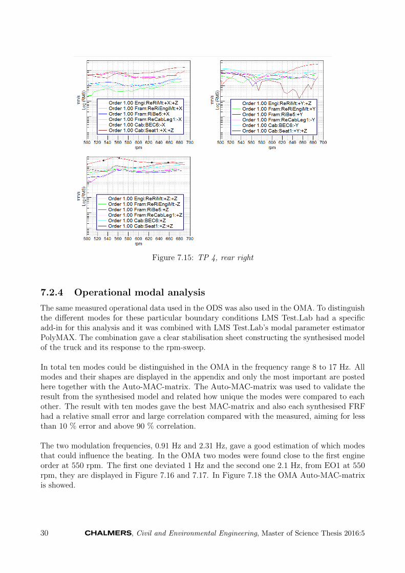
Figure 7.15: TP 4, rear right

7.2.4 Operational modal analysis

The same measured operational data used in the ODS was also used in the OMA. To distinguishthe di↵erent modes for these particular boundary conditions LMS Test.Lab had a specificadd-in for this analysis and it was combined with LMS Test.Lab’s modal parameter estimatorPolyMAX. The combination gave a clear stabilisation sheet constructing the synthesised modelof the truck and its response to the rpm-sweep.

In total ten modes could be distinguished in the OMA in the frequency range 8 to 17 Hz. Allmodes and their shapes are displayed in the appendix and only the most important are postedhere together with the Auto-MAC-matrix. The Auto-MAC-matrix was used to validate theresult from the synthesised model and related how unique the modes were compared to eachother. The result with ten modes gave the best MAC-matrix and also each synthesised FRFhad a relative small error and large correlation compared with the measured, aiming for lessthan 10 % error and above 90 % correlation.

The two modulation frequencies, 0.91 Hz and 2.31 Hz, gave a good estimation of which modesthat could influence the beating. In the OMA two modes were found close to the first engineorder at 550 rpm. The first one deviated 1 Hz and the second one 2.1 Hz, from EO1 at 550rpm, they are displayed in Figure 7.16 and 7.17. In Figure 7.18 the OMA Auto-MAC-matrixis showed.


(a) Mode one OMA, 8.2 Hz phase 0 �

(b) Mode one OMA,8.2 Hz phase 180 �

Figure 7.16: Mode one, 8.2 Hz, Engine roll and yaw (small). Cab roll (small)


(a) Mode five OMA, 11.3 Hz phase 0 �

(b) Mode five OMA, 11.3 Hz phase 180 �

Figure 7.17: Mode five, 11.3 Hz, Engine pitch


Figure 7.18: MAC-matrix for the OMA mode set

7.2.5 Discussion operational measurement

The results in Section 7.2.2 show that the deflection of the di↵erent subsystems of the truckwas greater for EO1 than EO3. The reason for this is probably that the engine mounts couldnot isolate these low frequencies. At idle rpm EO1 was equal to 9.2 Hz and EO3 equals 27.6 Hz.The simulation of only the engine itself showed that the rigid body modes of the engine wasspread out between 6 to 17 Hz, which also strengthens the theory of the rather low isolation ofthe first engine order through the engine mounts.

It can be seen in Figure 7.14 that the vibration level in x-direction increased between Fram:LeBe5and Fram:LeCabLeg1 which implies that the cab anchorage was sensitive to first engine ordervibrations in the x-direction.

Looking at the first engine order response of the truck, Figure 7.6 the peak at 557 rpm whichimplies that the behaviour might be resonant.

In total ten modes were found in the OMA and two of them corresponded quite well with thetwo di↵erent modulation frequencies found earlier. The MAC-matrix showed that the foundmodes are quite unique, not 100 % but they are clearly separated from each other.

One should bear in mind that the damping in a complete truck is very high. Therefore thefrequency response for this type of excitation is quite flat compared to, if only a decoupled cabstructure or chassis had been excited.


8 Modal measurements

Modal analysis measurements were carried out using the so called road simulator rig, whichbasically is an arrangement of several hydraulic pillars that the truck is placed onto. Thetruck stood with its four wheels on large concave steel plates, see Figure 8.1 and 8.2, that wasattached to the top of the hydraulic pillars. The steel plates allows for some movement in thelateral direction. The pillars were then exciting the structure in a certain manner, in this casesinusoidal sweeps. To control the output signal one can either chose to control the output forceor the displacement of the pillar. Displacement control was chosen for this setup, the decisionwas based on the information and knowledge of the rig operator that the rig performs best inthis configuration.

To achieve a good excitation of the truck the parking brake was released, knowledge from therig-operator. This let the wheel axles move freely in all directions compared to having theparking brake engaged. The truck was not secured to the rig in any way more than its ownweight and the concave steel plates that make sure that it did not roll of. This ensured a goodexcitation and boundary conditions similar to the reality. However, this limited the accelerationamplitude that could be used for the excitation. Too high acceleration will cause the wheel tolose contact with the steel plate and at that moment it is no longer a sinusoidal excitation. Thisalso limited the amplitude of the displacement and the sweep rate used. All these three parame-ters were tuned in before the measurements. Looking at the signal of the displacement and theforce revealed if the wheel had lost contact with the plate. Another way would be to manuallycheck, both by visual checks and listening to the excitation; if it loses contact it starts so clatter.

Figure 8.1: Front wheel plate Figure 8.2: Rear wheel plate

8.1 Methodology - Modal analysis

8.1.1 Excitation - Sinusoidal sweep

The excitation of the truck was done by the hydraulic pillars as described above and the signaltype was sinusoidal sweep between 5 and 20 Hz. White noise was also tested as excitationsignal but was not able to input enough energy to the structure which lead to a bad frequencyresponse function and low coherence. The frequency range was limited by two major factors;


The lowest possible frequency was 5 Hz due to that the control of the output signal in Test.Labwas 5 Hz. The upper limit was set by the rig itself and the hydraulic pumps, because there isa trade o↵ in frequency range, displacement and input force.In addition to the limit of maximum input force in the excitation, described earlier in Section8 the force was also limited due to the chosen sweep rate, [Hz/s]. Too high sweep rate alsocause the wheel to lose contact with the steel plate. A narrow frequency range of the sweepwas easier to configure with respect to achieving a good sinusoidal sweep. Therefore the upperlimit was set to 20 Hz, which also corresponds well with the specified upper limit from theprerequisites.

8.1.2 Data acquisition

The sinusoidal sweep was set from 5 to 20 Hz with a sweep rate of 0.25 Hz/s. It was equallyimportant in this measurement that the resolution was good for the analysis why it wasset to 0.1 Hz. The sampling frequency was 100 Hz and each block was then equal to 10seconds. The total length of the sinusoidal sweep is 60 seconds and the acquisition set-tings were made to fit an even number of block into the total sweep time, in this case sixblocks. In total five sweeps per setup were measured and used to achieve a stable averaged FRF.

A selection of measurement positions and their corresponding FRFs and coherences are shownin Figure 8.3 and 8.4, position Cab:Seat1, Fram:CabLeg1 and Engi:ReRiMt. They displaythe general shape of the FRF:s, i.e mostly damped and with a few anti-resonances, theanti-resonances correlates with the dips in the coherence curves, which is correct since lowacceleration in the structure leads to bad coherence.


Figure 8.3: FRF-curves for engine, chassis and cab positions

Figure 8.4: Coherence-curves for engine, chassis and cab positions


8.2 Results Modal measurements

The result of the modal analysis was directly comparable to the simulated modal analysis,presented in Section 5. Both methods displayed the resonant behaviour of the truck withoutthe engine as a driving source, which was the case in the operational analyses.

In total 12 modes were found in the modal analysis. They were a combination of rigid bodymodes (RBM) and flexural modes for the di↵erent subsystems. For the engine the threedi↵erent rotational RBMs were all fund; roll, pitch and yaw, however the three translational;Surg, Sway and bounce, were not located. Also at the cab three RBMs were excited; roll, yawand sway, a mixture of rotational and translational RBMs. Looking at the front wheel axle theroll and surging modes were found. In the chassis four flexural modes were located and noRBMs. The flexural modes were oriented both in the vertical and horisontal direction.

Comparing the resonance frequencies of the 12 modes and the deviation from EO1 gave intotal four modes that correlated well with the two modulation frequencies. They were modeno. 3, 4, 6 and 7. No. 3 and 7 corresponded to modulation frequency 2.31 Hz and no. 4 and 6to 0.91 Hz. The modes are displayed in Figure 8.5, 8.6, 8.7 and 8.8.


(a) Mode three, 6.9 Hz, phase 0 �

(b) Mode three, 6.9 Hz, phase 180 �

Figure 8.5: Modal mode three, 6.9 Hz, cab yaw engine close to bounce


(a) Mode four, 7.9 Hz, phase 0 �

(b) Mode four, 7.9 Hz, phase 180 �

Figure 8.6: Modal mode four, 7.9 Hz,Cab roll


(a) Mode six, 10.4 Hz, phase 0 �

(b) Mode six, 10.4 Hz, phase 0 �

Figure 8.7: Modal mode six, 10.4 Hz, Engine yaw, cab yaw (out of phase)


(a) Mode seven, 11.7 Hz, phase 0 �

(b) Mode seven, 11.7 Hz, phase 0 �

Figure 8.8: Modal mode seven, 11.7 Hz, Front axle roll, engine roll (small)


The quality of the selected mode set is presented in the Auto-MAC-matrix in Figure 8.9.One can clearly see that the modes were less dependent of each other in the modal analysiscompared to the OMA, except for the first three modes, which were similar to each other.Independent modes implied that the measurements together with the synthesised model wasgood and displayed a valid representation of the modal system.

Figure 8.9: Auto-MAC-matrix, Modal analysis

A comparison between some synthesised and measured FRFs are plotted in Figure 8.10, 8.11and 8.12 and show the quality of the synthesised model in the experimental modal analysis.Vertical lines in the figures show the location of the stable poles, i.e the modes in the system.Red curve is the measured FRF and green is the synthesised one. The overall aim was toachieve a correlation higher than 90% and error less than 10%, note that they should not addup to 100% together.


Figure 8.10: Synthesis in Cab:Seat1

Figure 8.11: Synthesis in Fram:CabLeg1


Figure 8.12: Synthesis in Engi:ReRiMt

8.3 Discussion modal analysis

The experimental modal analysis revealed that the simulated modes, presented in Section 5,were very similar to the modal analysis. The amount of modes found in both methods in thefrequency range 0 to 12 Hz were more or less identical to each other, most of them also veryclose in frequency, 0.2 Hz, which was a satisfying deviation in an analysis of a complete truck.Above 12 Hz the experimental modal analysis missed some modes, mainly flexural modes of thechassis, compared with the simulated results. This could be due to the type of excitation of thetruck in the modal analysis. Neither of the two methods could be seen as the absolute correctmethod. Both has their advantages and disadvantages. The experimental modal analysis isbased on an real structure compared to the finite element model in the simulation; boundaryconditions are more complex in the reality but are also the real ones. One obvious di↵erenceis the response of the truck’s tires and their response was seen as linear in the model but inreality they are not linear. This might lead to overtones of the excitation frequency transferredto the structure. In total the simulated modal analysis resulted in 20 modes found, comparedwith the 12 modes found in the experimental modal analysis. However, within the most crucialrange, 6 to 12 Hz, the experimental modal analysis and the simulated results were comparable,which was a satisfying result.


9 Mode-map

Table 9.1 displays the experimental analysis methods used in the project. In the left columnthe geometrical mode shape is listed and in the following columns the specific frequency ofeach mode is stated, if the mode type is found in the analysis. The advantage of the mode-mapis that the same geometrical mode shape and frequency can be compared between the di↵erentanalysis methods used, which show the di↵erence between methods but also their correlation.OMA, operational modal analysis and EMA, experimental modal analysis. The results of thesimulated analysis cannot be published with regard to secrecy.

Mode shape OMA [Hz] EMA [Hz]Engine bounce - 6.9Engine sway 8.6 -Engine surg 16.4 -Engine yaw - 10.4Engine roll 8.2; 14.8; 15.8; 16.4; 16.91; 16.92 5.7Engine pitch 9.3; 10.9; 11.3 8.7Cab bounce - -Cab sway - 6.1; 13.0Cab surg - -Cab yaw - 6.9; 10.4Cab roll 14.8 7.9Cab pitch - 17.9FrWhAx roll - 11.7FrWhAx surg - 17.1FrWhAx sway - -FrWhAx bounce - -Chassis torsional 9.3 8.7Chassis bending vertical - 13.0; 14.2; 17.1Chassis bending horisontal - 8.7; 14.2; 15.4; 17.9ReWhAx yaw - -ReWhAx bounce - -

Table 9.1: Mode map, all used methods put together

10 Discussion

There is always an uncertainty whether subjectively detected vibrations and phenomena likebeating can be objectively quantified and coupled to each other with accuracy. However,a beating phenomenon was visible in the time signal of the measurement position on theseat base, Cab:Seat1. It was also most prominent in the x-direction which also was the casewhen one is subjectively feeling the beating. A small pushing e↵ect in the back rest of the


seat, in x-direction. Not only one but two modulation frequencies were found in the analysis,which could explain the perceived di↵erence in modulation frequency over time. These twofrequencies repeated themselves over time regardless of temperature. It was the same whensubjectively evaluating the room temperature situation. With a warm engine the spectrumwas clearer and also more stable. Since the di↵erent modulation frequencies were found it isprobably not only one but two resonances that that need to be located in the e↵ort to findthe reasons for the beating phenomenon in the cab seat vibrations. The modulation frequen-cies 0.91 Hz and 2.31 Hz were not clear harmonics of each other. Therefore it is most likelythat it is two or more resonances that shall be found rather than one as the initial guess implied.

Hence, it was of interest to find resonances in the frequency region 6 to 12 Hz which correspondedto EO1 plus minus 2.31 Hz with some extra margin at the limits, which also covers the 0.91 Hzmodulation frequency. In Table 10.1 each mode with its shape and frequency that correspondsto the above specified frequency range are listed. The table is a smaller version of the completemode map. The results show that ten modes fit the smaller frequency range. The distinctfrequencies that corresponded to the deviation to EO1 at idle, 9.2 Hz, are; 6.9, 8.3, 10.1 and11.5 Hz. Those modes that match the modulation frequencies are written in boldface in Table10.1.The correlation between the experimental and simulated modal analysis was good, withinthe 6 to 12 Hz range the maximum deviation was 1.6 Hz. Comparing the operational modalanalysis, the experimental modal analysis and the finite element modal analysis the last two,EMA and FE-Compl. truck, corresponded better to each other than the OMA did. This isdue to that the engine when running is an energy source, in the OMA case, but in the EMAand FE-Compl. truck case, the engine is just a mass with springs and damping. They displaytwo di↵erent behaviours, the resonant and the driven one.

Mode shape OMA [Hz] EMA [Hz]Engine bounce - 6.9Engine sway 8.6 -Engine yaw - 10.4Engine roll 8.2 11.7Engine pitch 11.3 8.7Cab yaw - 6.9; 10.4Cab roll 8.2 7.9FrWhAx roll - 11.7Chassis bending - 8.7Chassis bending vertical - -Chassis bending horisontal - 8.7

Table 10.1: Smaller mode-map, representing the smaller frequency range 6-12 Hz

Both methods, operational and modal, were relevant since they displayed di↵erent behaviours ofthe structures, the driven and the resonant. They also displayed two di↵erent analysis methods.In the operational case the extracted modes and deformations were a relation between thereference position and other positions, transmissibilities. Compared with the modal case wherethe response was normalised to a known input force. It was therefore not surprising that thetwo methods displayed di↵erent mode shapes at di↵erent frequencies.


To minimise one of the non-linearities of the rubber in the engine mounts the temperature wasmonitored during the test, at the rear right engine mount, and the truck was pre-heated beforeall measurements. This should minimise the di↵erence between the operational and modalmeasurements regarding the damping and sti↵ness properties of the engine mounts. Since thiswas believed to have an e↵ect on the comparison of the di↵erent methods.

The modal validation of both EMA and OMA regarding synthesised FRFs compared withmeasured were satisfying for almost all nodes, except for a few positions on the cab and mostlyin the OMA where the adaptation was poor. This was due to that the real FRFs did not con-tain clear modal peaks, but was rather flat, since the complete truck contained a lot of damping.

As shown in Section 7 the vibration level of EO1 was higher on the cab side of the cab anchoragethan on the chassis side close to the cab anchorage. It was also clear that the cab anchoragehad a higher deflection in the x-direction which was necessary if a yaw motion was to bepresent, i.e as several of the resonant modes close to EO1 had. The higher vibration levelscould therefore be due to the modal behaviour of the cab. It also implied that the modalbehaviour of the cab was due to the weakness in the cab anchorage. The 6.9 Hz resonance inthe experimental modal analysis displayed the yaw motion of the cab and this resonance wasalso one that corresponded to the 2.3 Hz modulation frequency. By changing the sti↵ness ofthe cab anchorage the resonance frequency of this mode could be altered, either up or down infrequency. Lowering the resonance frequency would move the resonance further away fromEO1 which might decrease the beating phenomenon.

The front wheel axle had a clear resonant behaviour at 11.7 Hz in the modal analysis butnot found in the OMA. The reason could be that during the operational measurements theparking brake was applied, but in the experimental modal measurements the parking brakewas released. This since the truck was placed on the concave steel, Figure 8.1 and 8.2, whichprevented the truck from moving. In the operational measurements the engagement of theparking brake was needed to prevent the truck from moving. This changed the rotationalproperties of the wheels and by that the modal behaviour was altered.

The engine was the subsystem that was the easiest to excite in the modal analysis and wherealmost all RBMs were found. However, there was a clear di↵erence between the modal andoperational case where the engine had a very driven behaviour. The motion at idle rpm wasdominated by the pitch and roll modes. The roll motion could be derived to EO3 becauseof the force transmission between the ignition and and the crankshaft. This was displayedin Figure 7.7 where the motion of EO3 is filtered from the rest. The pitch motion was notas clear as the roll but it depended quite much on EO1 as seen in Figure 7.5. One shouldalso remember that this was transmissibilities, which is a relation between the accelerationmeasured at the truck. The resonant behaviour can still be vital even though its modes wasnot visible in the OMA. Therefore the two di↵erent methods complement each other well andprovide useful information.


11 Conclusion

It was found that the subjectively determined beating in the cab seat could be measured andthat the behaviour, regarding coordinate direction, was the same. The beating was strongestin x-direction. Not only one but two modulation frequencies were found, 0.91 Hz and 2.31 Hz,see Section 7.2.1.

As reported in Section 9 the di↵erent methods used in the project have together shown thatthere existed modes in the truck’s di↵erent subsystems that correlated with the two modulationfrequencies found. In total ten di↵erent mode shapes fit the 6 to 12 Hz interval and five ofthose; engine bounce, engine roll, cab yaw, cab roll, chassis bending horisontal, match themodulation frequencies. It was therefore at this stage not possible to specify one specific modethat was most responsible for the beating phenomena without further investigations. Therewas also the possibility that they were all needed to create the beating.

From the comparison between the simulated and experimental modal analysis it could be saidthat the correlation between FEM and EMA was good. In the 0 to 20 Hz range the maximumdeviation for one mode was 6.6 Hz but in the 6 to 12 Hz ,which was the most interesting, thedeviation was only 2.3 Hz. Several of the modes deviated less then 1 Hz in both ranges and anexact match was also found in a couple of cases. By those results the performed experimentalmodal analysis was concluded to output reliable mode shapes and frequencies.

The results are limited to the specific test truck used in this project and cannot be applied ona general truck. In general, beating phenomenon can appear when one or several subsystems,containing a number of resonances, are coupled and subjected to a vibrational force. In theproject only one loop of measurements has been carried out and therefore no attempts tochange the modal behaviour of, for example the cab anchorage, has been performed.

12 Future work

The project resulted in a number of conclusions but also raised new questions that could not beanswered by the measurements and analysis conducted. In the future it would be interestingto evaluate a design change of the cab anchorage to confirm the conclusion of that the cab yawmode at 6.9 Hz is responsible for the beating with 2.3 Hz modulation frequency. This could bedone by either sti↵en the cab anchorage or make it weaker in order to change the resonancefrequency. It would also be interesting to further analyse the vibration pattern in the driverseat more in detail and try to determine why the vibration level of EO1 is increased in thedriver seat position in the operational measurements.


References

[1] Advanced transfer path analysis techniques. Siemens.[2] Peter Avitabile. Experimental modal analysis - A simple non mathematical presentation.

Sound and Vibration (2001).[3] Anders Brandt. Noise and vibration analysis - Signal anlysis and Experimental procedures.

John Wiley & Sons, Ltd, 2011.[4] Christof Devriendt, Gert De Sitter, Steve Vanlanduit, and Patrick Guillaume. Operational

modal analysis in the presence of harmonic excitations by the use of transmissibilitymeasurements. Sound and Vibration (2009).

[5] Michael J. Gri�n. A comparison of standardized methods for predicting the hazards ofwhole body vibration and repeted shocks. Sound and Vibration (1998).

[6] Grundlaggande fordonsteknik - Lastvagnar. Volvo Truck Parts AB, 1991.[7] Handbook of human vibration. Harcourt Brace & Company, 1990.[8] How to performe transfer path analysis. Siemens.[9] Jacek Kromulski and Edward Hojan. An application of two experimental modal analysis

methods for the determination of operational deflection shapes. Sound and Vibration(1996).

[10] Wolfgang Kropp. Technical acoustics - Lecture note 4. Department of Applied Acoustics,Chalmers University of Technology. 2007.

[11] Prasenjit Mohanty and Daniel J. Rixen. Operational modal analysis in the presence ofharmonic excitation. Sound and Vibration (2002).

[12] Juha Plunt. Finding and fixing vehicle NVH problems with transfer path analysis. Soundand Vibration (2005).

[13] Psychoacoustics - Facts and models. Springer-Verlag, 1990.[14] Structure - Operational modal analysis.[15] Transfer Path Analysis - The qualificatioin and quantification of vibro-acoustic transfer

paths. Siemens.


A Measurement positions & Geometry

Engi EngineCab CabFram The two major chassis beamWhAx Wheel AxleStWh Steering WheelShaft Cardan shaftSubF The crossbeam under the front of the engine,

where the two front engine mounts are connectedLe LeftRi RightFr FrontRe RearBe BeamMt MountLEC Left End CabREC Right End CabFEC Front End CabBEC Back End Cab

Table A.1: List of abbreviations used in the geometry to name the measurement positions

Figure A.1: Measurement positions on the chassis


Figure A.2: Measurement positions on the engine

Figure A.3: Measurement positions on the cab


Figure A.4: Measurement positions on wheel axles, cardan shaft and the cross beam under thefront of the engine


B Operational modal analysis modes

Here are all the modes that were found in the OMA but not displayed in the result sectionsince they were not that vital for the beating phenomena.

(a) Mode two, 8.6 Hz, phase 0 �

(b) Mode two, 8.6 Hz, phase 0 �

Figure B.1: OMA mode two, 8.6 Hz


(a) Mode three, 9.3 Hz, phase 0 �

(b) Mode three, 9.3 Hz, phase 180 �

Figure B.2: OMA mode three, 9.3 Hz


(a) Mode four, 10.9 Hz, phase 0 �

(b) Mode four, 10.9 Hz, phase 180 �

Figure B.3: OMA mode four, 10.9 Hz


(a) Mode six, 14.8 Hz, phase 0 �

(b) Mode six, 14.8 Hz, phase 180 �

Figure B.4: OMA mode six, 14.8 Hz


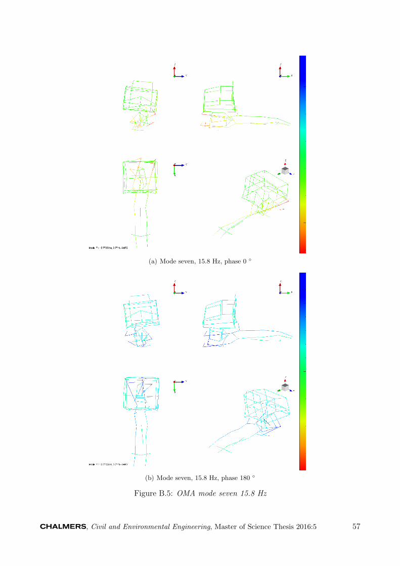
(a) Mode seven, 15.8 Hz, phase 0 �

(b) Mode seven, 15.8 Hz, phase 180 �

Figure B.5: OMA mode seven 15.8 Hz


(a) Mode eight, 16.4 Hz, phase 0 �

(b) Mode eight, 16.4 Hz, phase 0 �

Figure B.6: OMA mode eight, 16.4 Hz


(a) Mode nine, 16.91 Hz, phase 0 �

(b) Mode nine 16.91 Hz, phase 180 �

Figure B.7: OMA mode nine, 16.91 Hz


(a) Mode ten, 16.92 Hz, phase 0 �

(b) Mode ten, 16.92 Hz, phase 180 �

Figure B.8: OMA mode ten, 16.92 Hz


C Experimental modal analysis modes

(a) Mode one, 5.7 Hz, phase 0 �

(b) Mode one, 5.7 Hz, phase 180 �

Figure C.1: Modal mode one, 5.7 Hz


(a) Mode two, 6.1 Hz, phase 0 �

(b) Mode two, 6.1 Hz, phase 180 �

Figure C.2: Modal mode two, 6.1 Hz


(a) Mode five, 8.5 Hz, phase 0 �

(b) Mode five, 8.5 Hz, phase 180 �

Figure C.3: Modal mode five, 8.5 Hz


(a) Mode eight, 13.0 Hz, phase 0 �

(b) Mode eight, 13.0 Hz, phase 180 �

Figure C.4: Modal mode eight, 13.0 Hz


(a) Mode nine, 14.2 Hz, phase 0 �

(b) Mode nine, 14.2 Hz, phase 0 �

Figure C.5: Modal mode nine, 14.2 Hz


(a) Mode ten, 15.4 Hz, phase 0 �

(b) Mode ten, 15.4 Hz, phase 180 �

Figure C.6: Modal mode ten, 15.4 Hz


(a) Mode eleven, 17.1 Hz, phase 0 �

(b) Mode eleven, 17.1 Hz, phase 180 �

Figure C.7: Modal mode eleven, 17.1 Hz


(a) Mode twelve, 17.9 Hz, phase 0 �

(b) Mode twelve, 17.9 Hz, phase 180 �

Figure C.8: Modal mode twelve, 17.9 Hz


Vibration characterisation of low frequency engine...

Documents

Transcript of Vibration characterisation of low frequency engine...