VIBRATION-BASED DAMAGE DETECTION FOR TIMBER BRIDGES

VIBRATION-BASED DAMAGE DETECTION FOR TIMBER BRIDGES

A Thesis Submitted to the College of

Graduate Studies and Research

in Partial Fulfillment of the Requirements

for the Degree of Master of Science

in the Department of Civil Engineering

University of Saskatchewan

Saskatoon, Canada

By

Cameron Jonathan Beauregard

© Copyright Cameron Jonathan Beauregard, August 2012. All rights reserved.

i

PERMISSION TO USE

In presenting this thesis/dissertation in partial fulfillment of the requirements for a

Postgraduate degree from the University of Saskatchewan, I agree that the Libraries of

this University may make it freely available for inspection. I further agree that permission

for copying of this thesis/dissertation in any manner, in whole or in part, for scholarly

purposes may be granted by the professor or professors who supervised my

thesis/dissertation work or, in their absence, by the Head of the Department or the Dean

of the College in which my thesis work was done. It is understood that any copying or

publication or use of this thesis/dissertation or parts thereof for financial gain shall not

be allowed without my written permission. It is also understood that due recognition

shall be given to me and to the University of Saskatchewan in any scholarly use which

may be made of any material in my thesis/dissertation.

Requests for permission to copy or to make other uses of materials in this

thesis/dissertation in whole or part should be addressed to:

Head of the Department of Civil Engineering

University of Saskatchewan

57 Campus Drive

Saskatoon, Saskatchewan, S7N 5A9

Canada

ii

ABSTRACT

Vibration-based damage detection (VBDD) methods are global response-based

methods that have the potential to provide valuable insight into the health of a structure.

Dynamic characteristics obtained through vibration testing, such as the natural

frequencies and their associated mode shapes, are directly related to both the stiffness

and the mass of the structure, which are both good indicators of damage. In a typical

application of VBDD methods, the vibration characteristics are obtained periodically to

detect small changes in the response, indicating damage over time. However, this

thesis considers using a snapshot of the vibration signature based on a single set of

measurements to detect specific types of damage by comparing the response with that

of other similar structures with known condition states.

Like many provinces, Saskatchewan currently has a large inventory of aging timber

bridges that are at or nearing the end of their service life. Many of these bridges are

experiencing decay of their substructure elements (piles, pile caps and abutments), yet

these are not always accessible for the inspector to identify. Furthermore, current

inspection methods require lengthy and thorough site visits to reliably assess the

condition of the timber bridge. Given the length of the current inspection methods and

the large inventory of timber bridges in the Saskatchewan road network, other

assessment tools are being sought.

iii

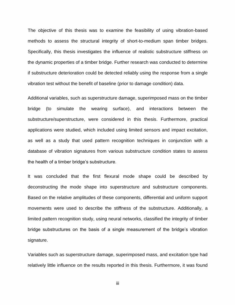
The objective of this thesis was to examine the feasibility of using vibration-based

methods to assess the structural integrity of short-to-medium span timber bridges.

Specifically, this thesis investigates the influence of realistic substructure stiffness on

the dynamic properties of a timber bridge. Further research was conducted to determine

if substructure deterioration could be detected reliably using the response from a single

vibration test without the benefit of baseline (prior to damage condition) data.

Additional variables, such as superstructure damage, superimposed mass on the timber

bridge (to simulate the wearing surface), and interactions between the

substructure/superstructure, were considered in this thesis. Furthermore, practical

applications were studied, which included using limited sensors and impact excitation,

as well as a study that used pattern recognition techniques in conjunction with a

database of vibration signatures from various substructure condition states to assess

the health of a timber bridge‟s substructure.

It was concluded that the first flexural mode shape could be described by

deconstructing the mode shape into superstructure and substructure components.

Based on the relative amplitudes of these components, differential and uniform support

movements were used to describe the stiffness of the substructure. Additionally, a

limited pattern recognition study, using neural networks, classified the integrity of timber

bridge substructures on the basis of a single measurement of the bridge‟s vibration

signature.

Variables such as superstructure damage, superimposed mass, and excitation type had

relatively little influence on the results reported in this thesis. Furthermore, it was found

iv

that substructure and superstructure damage could be detected independently;

however, superstructure damage detection required a baseline response.

v

ACKNOWLEDGEMENTS

I would like to express my gratitude to my supervisors, Dr. Bruce Sparling and Dr. Leon

Wegner, for their continual encouragement and guidance throughout the assembly of

my thesis. Your support and feedback have, undoubtedly, given me the motivation to

overcome the struggles of this undertaking.

I would also like to thank Saskatchewan Ministry of Highways and Infrastructure, as well

as the Natural Sciences and Engineering Research Council of Canada for their financial

support to complete this thesis. Additionally, I would like to thank the University of

Saskatchewan and Dr. Mel Hosain for their support through scholarships.

I acknowledge the help provided by my committee members, Drs. Jit Sharma, Doug

Milne, Lisa Feldman, and Mohamed Boulfiza, as well as the external examiner, Mark

Gress. Their feedback has greatly helped in the assembly of the thesis.

I would also like to acknowledge the assistance of Brennan Pokoyoway and Dale

Pavier, University of Saskatchewan Structures Laboratory technicians. I am also

thankful for all the other graduate students that helped me with my project, either

directly with the research, or indirectly with much needed distractions.

Finally, I would like to extend my gratitude to my family, friends, and my wife, Danae, for

the constant love and support. I am continuously grateful that I have been surrounded

by such amazing people.

vi

TABLE OF CONTENTS

PERMISSION TO USE .................................................................................................... i

ABSTRACT ......................................................................................................................ii

ACKNOWLEDGEMENTS ............................................................................................... v

TABLE OF CONTENTS ..................................................................................................vi

LIST OF TABLES ........................................................................................................... xii

LIST OF FIGURES ........................................................................................................ xvi

LIST OF SYMBOLS ..................................................................................................... xxii

LIST OF ABBREVIATIONS ......................................................................................... xxiv

1. INTRODUCTION ...................................................................................................... 1

1.1. BACKGROUND ................................................................................................. 1

1.2. OBJECTIVES ..................................................................................................... 3

1.3. SCOPE AND METHODOLOGY ......................................................................... 4

1.4. LAYOUT OF THESIS ......................................................................................... 5

2. LITERATURE REVIEW ............................................................................................ 7

2.1. INTRODUCTION ................................................................................................ 7

2.2. TIMBER BRIDGES ............................................................................................ 7

vii

2.2.1. Timber Characteristics ................................................................................. 7

2.2.2. Saskatchewan Timber Bridges .................................................................. 10

2.3. VIBRATION-BASED DAMAGE DETECTION .................................................. 11

2.3.1. Overview .................................................................................................... 11

2.3.2. VBDD Techniques ..................................................................................... 12

2.3.3. VBDD Research at the University of Saskatchewan ................................. 15

2.3.4. VBDD with Timber ..................................................................................... 16

2.3.5. Further VBDD on Substructures ................................................................ 20

3. DESCRIPTION OF EXPERIMENTAL STUDY........................................................ 21

3.1. INTRODUCTION .............................................................................................. 21

3.2. TIMBER BRIDGE ............................................................................................. 21

3.3. EXCITATION .................................................................................................... 24

3.3.1. Overview .................................................................................................... 24

3.3.2. Impact ........................................................................................................ 24

3.3.3. Hydraulic Shaker ....................................................................................... 25

3.3.4. Summary ................................................................................................... 26

3.4. ACCELEROMETERS ...................................................................................... 26

3.5. DATA PROCESSING AND TESTING PROTOCOL ......................................... 29

3.5.1. Overview .................................................................................................... 29

3.5.2. Data Acquisition ......................................................................................... 29

viii

3.5.3. Signal Processing ...................................................................................... 30

3.6. PRELIMINARY TESTS TO DEFINE TEST PROTOCOLS ............................... 34

3.6.1. Overview .................................................................................................... 34

3.6.2. Interference Between Lower Modes .......................................................... 34

3.6.3. Methods for Accentuating the First Flexural Mode .................................... 36

3.7. DAMAGE CASES CONSIDERED .................................................................... 38

3.7.1. Overview .................................................................................................... 38

3.7.2. Determination of Substructure Stiffness .................................................... 39

3.7.3. Substructure Damage Cases ..................................................................... 47

3.7.4. Weight Cases ............................................................................................ 48

3.7.5. Superstructure Damage Cases ................................................................. 50

3.8. SUMMARY OF THE EXPERIMENTAL PROGRAM ......................................... 51

3.8.1. Overview .................................................................................................... 51

3.8.2. Substructure Damage Program ................................................................. 53

3.8.3. Weight Case program ................................................................................ 53

3.8.4. Substructure and Superstructure Interaction Program .............................. 53

4. TIMBER BRIDGE DAMAGE DECTECTION RESULTS ......................................... 54

4.1. INTRODUCTION .............................................................................................. 54

4.2. BRIDGE BEHAVIOUR ..................................................................................... 54

4.2.1. Overview .................................................................................................... 54

ix

4.2.2. Dynamic Response ................................................................................... 55

4.2.3. Normalization ............................................................................................. 59

4.2.4. Mode Shape Variability .............................................................................. 63

4.2.5. Mode Shape Components ......................................................................... 65

4.2.6. Summary ................................................................................................... 68

4.3. DETECTION OF SUBSTRUCTURE DAMAGE TO A SINGLE SUPPORT ...... 68

4.3.1. Overview .................................................................................................... 68

4.3.2. Uniform Substructure Deterioration ........................................................... 69

4.3.3. Local Substructure Deterioration ............................................................... 72

4.3.4. Quantitative Analysis with Mode Shape Components ............................... 74

4.3.5. Effect of Excitation ..................................................................................... 77

4.3.6. Natural Frequency ..................................................................................... 80

4.3.7. Summary ................................................................................................... 82

4.4. SUBSTRUCTURE DAMAGE DETECTION ON BOTH SUPPORTS ................ 82

4.4.1. Overview .................................................................................................... 82

4.4.2. Results and Discussion ............................................................................. 83

4.4.3. Summary ................................................................................................... 85

4.5. INFLUENCE OF SUPERIMPOSED MASS ...................................................... 85

4.5.1. Overview .................................................................................................... 85

4.5.2. Results and Discussion ............................................................................. 86

x

4.5.3. Summary ................................................................................................... 88

4.6. SUPERSTRUCTURE DAMAGE DETECTION ................................................. 89

4.6.1. Overview .................................................................................................... 89

4.6.2. Superstructure Damage Detection ............................................................ 89

4.6.3. Substructure and Superstructure Interactions ........................................... 92

4.6.4. Summary ................................................................................................... 99

4.7. PRACTICAL APPLICATION ............................................................................ 99

4.7.1. Overview .................................................................................................... 99

4.7.2. Results and Discussion ........................................................................... 100

4.7.3. Summary ................................................................................................. 104

5. PATTERN RECOGNITION USING NEURAL NETWORKS ................................. 105

5.1. OVERVIEW .................................................................................................... 105

5.2. BACKGROUND ............................................................................................. 105

5.3. EXPERIMENTAL PROGRAM ........................................................................ 107

5.4. RESULTS....................................................................................................... 110

5.5. CONCLUSION ............................................................................................... 112

6. CONCLUSIONS AND RECOMMENDATIONS ..................................................... 113

6.1. SUMMARY ..................................................................................................... 113

6.2. CONCLUSIONS ............................................................................................. 114

6.3. RECOMMENDATIONS AND FUTURE RESEARCH ..................................... 117

xi

REFERENCES ............................................................................................................ 118

APPENDIX A. SIGNAL PROCESSING ....................................................................... 125

APPENDIX B. OBTAINING SUBSTRUCTURE STIFFNESS ...................................... 129

APPENDIX C. NORMALIZED MODE SHAPES .......................................................... 131

APPENDIX D. MODE SHAPE COMPONENTS .......................................................... 139

APPENDIX E. NATURAL FREQUENCIES ................................................................. 146

APPENDIX F. VIBRATION-BASED DAMAGE DETECTION ...................................... 148

APPENDIX G. STATISTICAL ANALYSIS ................................................................... 154

xii

LIST OF TABLES

Table 3.1. Excitation methods ....................................................................................... 26

Table 3.2. Definition of the three accelerometer configurations .................................... 28

Table 3.3. Foundation stiffness window (per pile) ......................................................... 44

Table 3.4. Substructure condition states ....................................................................... 47

Table 3.5. Summary of the weight cases considered .................................................... 50

Table 3.6. Superstructure condition states .................................................................... 51

Table 4.1. Change in mode shape components relative to the base foundation case

(D0S0W1a) for multiple foundation cases, using two excitation methods ............. 79

Table 4.2. Fundamental frequency of the bridge for different softening cases under a

single support. ...................................................................................................... 81

Table 4.3. Fundamental frequency of the bridge for cases with damage to both supports

.............................................................................................................................. 84

Table 4.4. Effect of weight on the fundamental frequency ............................................. 88

Table 4.5. Change in mode shape components relative to the base foundation case

(D0S0W1a), for impact loading considering 22 sensors vs. 12 sensors ............. 103

Table 5.1. Mode shape component data used to train the model ................................ 109

Table 5.2. Mode shape component data used to test the model ................................. 109

Table A.1. Acceleration calibration factors from different dates .................................. 126

Table B.1. Summary of stiffness of pile below ground stiffness, ks ............................. 130

xiii

Table C.1. Unit-norm mode shape for D0S0W1a from harmonic and impact excitation

............................................................................................................................ 132

Table C.2. Unit-norm mode shape for D1S0W1 from harmonic and impact excitation 132



Table C.5. Unit-norm mode shape for D0S0W1b from harmonic and impact excitation

............................................................................................................................ 133



............................................................................................................................ 134


Table C.9. Unit-norm mode shape for D0S0W1c from harmonic and impact excitation

............................................................................................................................ 134


............................................................................................................................ 135

Table C.11. Unit-norm mode shape for D5S0W1 from harmonic and impact excitation

............................................................................................................................ 135


............................................................................................................................ 135


............................................................................................................................ 136


............................................................................................................................ 136

xiv


............................................................................................................................ 136


............................................................................................................................ 137


............................................................................................................................ 137


............................................................................................................................ 137


............................................................................................................................ 138


............................................................................................................................ 138

Table D.1. Summary of average mode shape components from harmonic excitation 140

Table D.2. Summary of average mode shape components from impact excitation ..... 143

Table E.1. Summary of all natural frequencies for timber bridge condition states ....... 147

Table F.1. Area under the change in mode shape plots when comparing similar

superstructure states to establish a threshold ..................................................... 153

Table F.2. Area under the change in curvature plots when comparing similar

superstructure states to establish a threshold ..................................................... 153

Table G.1. T-test results considering bridge states with varying substructure stiffness

under a single support ........................................................................................ 155

Table G.2. F-test on variance results considering bridge states with varying substructure

stiffness under a single support .......................................................................... 156

xv


under both supports ............................................................................................ 157


and superimposed mass ..................................................................................... 158

Table G.5. T-test results considering bridge states with similar substructure stiffness

(D0) and varying superstructure states ............................................................... 159








and varying superstructure states ....................................................................... 161


under a single support using the limited accelerometer configuration ................ 162

xvi

LIST OF FIGURES

Figure 1.1. Timber bridge (courtesy of Yang Sun) .......................................................... 1

Figure 1.2. A timber substructure (courtesy of Stantec Inc.) ........................................... 2

Figure 2.1. Diagram showing where decay is most likely to occur on a timber bridge

(after Ritter 1990; RTA 2008; Muchmore 1986) ...................................................... 9

Figure 3.1. The timber bridge in the laboratory ............................................................. 22

Figure 3.2. Plan view and cross-section of the timber bridge (dimensions in mm) ........ 23

Figure 3.3. The hydraulic shaker on the timber bridge .................................................. 25

Figure 3.4. Accelerometer ............................................................................................. 27

Figure 3.5. Plan view of the bridge deck, showing the location of accelerometers and

excitation (dimensions in mm) .............................................................................. 28

Figure 3.6. Data processing flow chart .......................................................................... 32

Figure 3.7. Comparison of the first torsional and first flexural mode shapes of the bare

bridge .................................................................................................................... 35

Figure 3.8. Partial frequency spectrum for the reference accelerometer obtained using

impact excitation, showing the closely spaced flexural and torsional modes ........ 36


impact excitation after the torsional mode was suppressed .................................. 38

Figure 3.10. Effective stiffness model by considering the soil-pile interaction of an

embedded timber pile ........................................................................................... 39

xvii

Figure 3.11 Typical applied load vs. average axial deflection behaviour for a timber pile

with highlighted low and high load pile stiffness (after Donovan 2004) ................. 41

Figure 3.12. Low load pile stiffness vs. high load pile stiffness, showing a range of

above ground pile stiffness, kp (data from Donavan 2004) ................................... 42

Figure 3.13. Range of soil-pile system stiffness below ground, ks ................................. 43

Figure 3.14. Wood block support setup (front and side views) ...................................... 44

Figure 3.15. Test setup to determine support stiffness ................................................. 45

Figure 3.16. Pine and oak block foundation load deflection curve (per support) ........... 46

Figure 3.17. Plan view of the deck, showing the distribution of concrete blocks used to

produce the two weight cases ............................................................................... 49

Figure 3.18. Timber bridge loaded with Weight Case 1 (W1) ........................................ 50

Figure 3.19. Summary of experimental program ........................................................... 52

Figure 4.1. Frequency spectrum of the reference accelerometer for foundation case

D0S0W1a using impact loading ............................................................................ 55

Figure 4.2. First flexural mode shape for foundation case D0S0W1a, obtained using

impact loading ....................................................................................................... 56

Figure 4.3. First flexural mode shape for foundation case D1S0W1, obtained using

impact loading ....................................................................................................... 57


impact loading ....................................................................................................... 57

Figure 4.5. Acceleration spectra showing the first flexural and torsional natural

frequencies under different damage states ........................................................... 58

xviii

Figure 4.6. Representations of the same mode shape using the (a) bridge- and (b)

girder-normalization schemes (generated using pseudo data) ............................. 61

Figure 4.7. Bridge-normalized representation of the soft foundation case (D2S0W1) ... 62

Figure 4.8. Girder-normalized representation of the soft foundation case (D2S0W1) ... 62

Figure 4.9. Variability of mode shape amplitudes for the base support case (D0) using

harmonic excitation ............................................................................................... 64


impact excitation ................................................................................................... 64

Figure 4.11. Mode shape of Girder 1 for foundation case D0S0W1 (harmonic

excitation), subdivided into its three components ................................................. 66





Figure 4.14. Mode shape components along each girder for girder-normalized data from

harmonic excitation (rigid foundation case D0S0W1a) .......................................... 71


harmonic excitation (hard foundation case D1S0W1) ........................................... 71


harmonic excitation (soft foundation case D2S0W1) ............................................ 72

Figure 4.17. Partial frequency spectrum for the reference accelerometer for foundation

case D3S0W1, showing the first torsional and flexural natural frequency separation

.............................................................................................................................. 73

xix

Figure 4.18. Mode shape components for girder-normalized data from harmonic

excitation (D3) ....................................................................................................... 73

Figure 4.19. Mode shape components for bridge-normalized data from harmonic

excitation (D3) ....................................................................................................... 74

Figure 4.20. Illustration of the standard chart used to summarize the mode shape

component data (produced using pseudo data) .................................................... 75

Figure 4.21. Mode shape components of girder-normalized data from harmonic loading

(D0, D1, D2, & D3) ................................................................................................ 76

Figure 4.22. Mode shape components for girder-normalized data from impact excitation

(D0, D1, D2, D3) ................................................................................................... 78


excitation (D0, D4, D5, D6) ................................................................................... 84

Figure 4.24. Mode shape components from harmonic excitation for different weight

cases .................................................................................................................... 87

Figure 4.25. Change in mode shape - D0S0W1c vs. D0S1W1 (harmonic) .................... 90

Figure 4.26. Change in curvature – D0S0W1c vs. D0S1W1 (harmonic) ........................ 90

Figure 4.27. Change in mode shape - D0S1W1 vs. D0S2W1 (harmonic) ..................... 91

Figure 4.28. Change in curvature – D0S1W1 vs. D0S2W1 (harmonic) ......................... 91

Figure 4.29. Change in mode shape - D0S1W1 vs. D0S2W1 (impact) ......................... 92

Figure 4.30. Change in curvature – D0S1W1 vs. D0S2W1 (impact) ............................. 92

Figure 4.31. Change in mode shape - D0S1W1 vs. D4S2W1 (harmonic) ..................... 93

Figure 4.32. Change in curvature – D0S1W1 vs. D4S2W1 (harmonic) ......................... 93

xx

Figure 4.33. Mode shape components for the bridge with a constant foundation case

D6, but under various superstructure condition states .......................................... 95

Figure 4.34. Area under the change in mode shape and change in curvature plots when

comparing the base case (D0S1W1) to other superstructure and substructure

damage states ...................................................................................................... 97

Figure 4.35. Area under the change in mode shape and change in curvature plots when

comparing the base case (D0S0W1) to other superstructure and substructure

damage states ...................................................................................................... 98

Figure 4.36. Plan view of the bridge, showing accelerometer locations for practical

application (dimensions in mm) .......................................................................... 101

Figure 4.37. First flexural mode shape produced using limited sensors ...................... 101

Figure 4.38. Mode shape components for substructure condition states using the limited

accelerometer configuration ................................................................................ 102

Figure 5.1. A simple artificial neural network (Gurney 1997) ....................................... 106

Figure 5.2. A.I. Solver user interface displaying results from both training and testing of

the neural network .............................................................................................. 110

Figure 5.3. Graphical representation of the hard and soft damage cases, and their

relationship to mode shape components „A‟ and „C‟ ........................................... 111

Figure D.1. Mode shape component amplitudes from harmonic excitation I ............... 141

Figure D.2. Mode shape component amplitudes from harmonic excitation II .............. 142

Figure D.3. Mode shape component amplitudes from impact excitation I ................... 144

Figure D.4. Mode shape component amplitudes from impact excitation II .................. 145

Figure F.1. Change in mode shape - D0S0W1c vs. D0S1W1 (harmonic) ................... 149

xxi

Figure F.2. Change in curvature – D0S0W1c vs. D0S1W1 (harmonic) ....................... 149







Figure F.9. Change in mode shape - D0S1W1 vs. D0S2W1 (harmonic)..................... 151

Figure F.10. Change in curvature – D0S1W1 vs. D0S2W1 (harmonic)....................... 151

Figure F.11. Change in mode shape - D0S1W1 vs. D4S2W1 (harmonic)................... 151






xxii

LIST OF SYMBOLS

A = Cross sectional area

d = Diameter

E = Modulus of Elasticity

EI = Bending stiffness

fi = Fundamental natural frequency (Hz)

G = Modulus of Rigidity

g = Acceleration due to gravity

k = System parameter for beam support conditions

k = Stiffness

ks = Stiffness of the portion of a pile located below ground

kp = Stiffness of the portion of a pile located above ground

keff = Effective substructure stiffness

L = Length of pile above ground

Ls = Length of pile extending below ground

R2 = Coefficient of determination

W = Uniformly distributed weight

α = Alpha, probability of making a type II error (false positive)

= Area under the change in mode shape vector

= Area under the change in curvature vector

ΔM = Added mass on the bridge

xxiii

= Change in mode shape vector

= Change in curvature vector

ζ = Radius of influence of pile

= Poisson‟s ratio

ω = Fundamental natural frequency (rad/s)

= Measured mode shape vector

= Mode shape vector after damage (normalized)

= Normalized mode shape vector

= Curvature vector after damage

= Curvature vector

= Bridge-normalized mode shape vector

= Girder-normalized mode shape vector

xxiv

LIST OF ABBREVIATIONS

A.I. Artificial Intelligence

Fdn Foundation

FFT Fast Fourier Transform

Labview Laboratory Virtual Instrumentation Engineering Workbench

NF Natural frequency

NI National Instruments

No. Number

SARM The Saskatchewan Association of Rural Municipalities

SHM Structural health monitoring

SHT Saskatchewan Highways and Transportation

Std Dev. Standard deviation

TM Trademark

Typ Typical

Ref Reference

VBDD Vibration-based damage detection

1

1. INTRODUCTION

1.1. BACKGROUND

Saskatchewan currently has a large inventory of timber bridges that are nearing or are

at the end of their service life. A typical timber bridge in Saskatchewan is short-to-

medium span, featuring simply supported girders and a timber deck. In some cases only

the substructure (consisting of piles, pile caps and abutments) is constructed out of

timber. Figure 1.1 presents a multi-span timber bridge spanning a long creek, while

Figure 1.2 presents a timber substructure under a bridge.

Figure 1.1. Timber bridge (courtesy of Yang Sun)

2

Figure 1.2. A timber substructure (courtesy of Stantec Inc.)

The structural health monitoring (SHM) program presently employed by transportation

agencies typically consists of lengthy visual inspections and minor non-destructive

testing. Visual inspections are limited to structural members that are directly accessible

to the inspectors, meaning that hidden deficiencies can remain undetected. These

deficiencies can be substantial and numerous due to a timber bridge‟s susceptibility to

many forms of deterioration, including weathering, rot, insect attack, and mechanical

damage. In many instances, the damage is inaccessible and is located at the foundation

in the form of pile rot at, or below, the ground surface. Given the large number of timber

bridges in Saskatchewan, and the difficulties associated with visual inspections, it would

be beneficial to have a method that would be capable of quickly detecting damage on a

timber bridge.

3

Vibration-based damage detection (VBDD) methods have the potential to offer great

insight into a structure‟s integrity when implemented into a routine structural health

monitoring program. The vibration-based methods measure the structure‟s dynamic

response to an excitation source using sensors. The characteristics obtained from

vibration measurements typically include natural frequencies and their corresponding

mode shapes, which can be used to assess a structure‟s health. Damage to the

structure presents itself in the form of changes in mass or stiffness, both of which affect

the vibration characteristics. Typically, the vibration characteristics of a structure must

be periodically measured to detect small changes in the response, indicating damage

that is occurring over time. However, it may also be possible to use specific vibration

signatures based on a single measurement to detect specific types of damage by

comparing the response with that of other structures with known condition states.

Specifically, preliminary studies have indicated that changes in the timber bridge

substructure (piles, pile caps and abutments) through deterioration affect the basic

character of the vibration mode shapes (Beauregard et al. 2010; Sun et al. 2007).

1.2. OBJECTIVES

The objective of this research project was to examine the feasibility of using vibration-

based methods to assess the structural integrity of short-to-medium span timber

bridges. Specific sub-objectives included the following:

To investigate the influence of substructure stiffness on the dynamic properties of

a timber bridge;

4

To determine if substructure deterioration can be detected reliably using the

response from a single vibration test without the benefit of baseline (prior to

damage condition) data;

To investigate the influence that the distributed mass supported by the bridge

deck has on the dynamic response of the timber bridge, given the non-linear

nature of timber;

To investigate the potential for VBDD methods to detect and locate small-scale

damage in the timber bridge superstructure;

To explore the relationship between substructure and superstructure damage

with particular attention paid to the ability to simultaneously detect damage to the

substructure and superstructure; and

To investigate the influence of various testing parameters that may be employed

in future field testing studies on timber bridges; more specifically, to assess

excitation sources and the degree of instrumentation required.

In addition to the sub-objectives above, this research also included a preliminary

investigation on the feasibility of using pattern recognition software to aid in determining

the condition state of a timber bridge given a database of vibration signatures of known

condition states.

1.3. SCOPE AND METHODOLOGY

The focus of this thesis was on the vibration testing of an intact portion of a

decommissioned timber bridge within a laboratory setting. The following variables were

analyzed individually to assess their effect on the bridge‟s dynamic response:

5

i. changes in support stiffness that were uniform across the bridge width;

ii. changes in localized support stiffness;

iii. changes in mass supported by the deck (to simulate a gravel driving

surface);

iv. a reduction in the flexural capacity of a girder; and

v. excitation methods.

Attempts were made to characterize the specific forms of damage using vibration-based

damage detection methods on the timber bridge. The effects of the specific variables

were assessed by analyzing the resulting natural frequencies and their associated

mode shapes. In addition, common VBDD methods were used for local damage

detection, including the change in mode shape method (Wegner et al. 2011) and the

change in curvature method (Pandey et al. 1991).

Investigations of both superstructure and substructure damage detection were

undertaken based on comparisons with the response using baseline measurements

taken at the bridge‟s original condition before the introduction of damage. In addition,

specific forms of substructure damage were thoroughly investigated to determine if they

could be detected by analyzing the vibration signatures obtained using a single vibration

measurement. Further details regarding the experimental program are provided in

Chapter 3.

1.4. LAYOUT OF THESIS

This thesis describes an experimental program and is presented in six chapters, plus

references and appendices. An overview of the chapters is presented below:

6

Chapter 1 served as an introduction that outlined the problem and the objectives of the

research.

Chapter 2 presents a literature review that summarizes past studies and literature

related to this research. Background relating to timber bridges and vibration based-

damage detection is presented.

Chapter 3 describes the experimental program. The laboratory timber bridge is

described, in addition to the excitation and data acquisition methods. Finally, Chapter 3

introduces the damage cases considered, which include the superstructure and

substructure damage cases.

Chapter 4 presents the main results of the research and provides some discussion. The

effect of substructure and superstructure damage, as well as distributed mass on the

dynamic response is studied. In particular, specific patterns in the mode shape profile

are identified.

Chapter 5 describes the results of a brief study that used pattern recognition techniques

to aid in predicting the state of a bridge using dynamic measurements. Based on a

database of timber bridge vibration signatures for known condition states, the condition

states of timber bridges were predicted.

Finally, Chapter 6 presents the conclusions of this study and subsequently outlines

recommendations for future research.

7

2. LITERATURE REVIEW

2.1. INTRODUCTION

This chapter is a summary of the past research relating to timber bridges and vibration-

based damage detection. Timber as a building material is described, with special

consideration of its use in bridge construction. An overview of the current state of

Saskatchewan‟s timber bridge network is also included.

The literature review concludes by providing a summary of research related to structural

health monitoring using vibration-based damage detection. Various vibration-based

damage detection methods are introduced, and their applications are presented. In

particular, the application of VBDD to bridge structures is presented, with a focus on

timber bridges and substructures.

2.2. TIMBER BRIDGES

2.2.1. Timber Characteristics

Timber is a highly sought-after building material due to its abundance as a renewable

resource. There are many benefits to using timber for construction purposes when a

proper design is implemented (Ou et al. 1986):

Construction can take place in any weather;

8

Timber is not affected by freeze-thaw cycles, or de-icing agents;

Timber has good energy-absorbing abilities;

Its light weight nature makes for easier construction, repair, and

rehabilitation; and

Capital and maintenance costs are competitive with other building

materials.

Timber, however, does have many limitations, making its use practical only for specific

bridge applications. Timber can degrade due to fungi, insects, marine borers,

discolorations, weathering, chemicals, and fire (Ou et al. 1986). Specifically, the biotic

agents such as decay, fungi, bacteria, insects, and marine borers require four

conditions for survival: (1) adequate moisture, (2) adequate oxygen, (3) favourable

temperature, and (4) food - the wood (Ritter 1990; Ou et al. 1986; Muchmore 1986).

These four factors are impossible to manage in a natural environment. However, the

wood may be treated by a chemical preservation that is toxic to organisms, thus

removing the food. Chemical treatment, however, can only penetrate the outer timber

shell, making the internal structure assessable to decay where moisture can enter.

Areas near fasteners, checks, and mechanical damage are highly susceptible to

damage as they provide paths where moisture can enter, especially when these are

also high moisture regions (RTA 2008; Ritter 1990). Figure 2.1 graphically shows the

areas most vulnerable to decay from moisture.

9

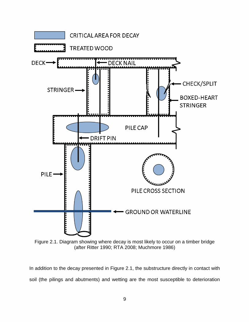
Figure 2.1. Diagram showing where decay is most likely to occur on a timber bridge

(after Ritter 1990; RTA 2008; Muchmore 1986)

In addition to the decay presented in Figure 2.1, the substructure directly in contact with

soil (the pilings and abutments) and wetting are the most susceptible to deterioration

10

(Ritter 1990). Unfortunately, the substructure can also be the most inaccessible, thus

presenting the most difficulty during inspections.

2.2.2. Saskatchewan Timber Bridges

Saskatchewan‟s municipal bridge network consists mainly of short-to-medium span

bridges constructed with some form of timber component. The Saskatchewan

Association of Rural Municipalities (SARM) has approximately 1900 rural bridges in the

Saskatchewan municipal bridge network, approximately 1700 of which have timber

abutments (this does not include the infrastructure in the highway bridge network). The

average construction date of these bridges was 1966. Additionally, the average

expected lifespan for this bridge inventory is 60 years based on the experience of

Saskatchewan Highways and Transportation (Watt et al. 2008).

The Saskatchewan Association of Rural Municipalities and Saskatchewan Highways

and Transportation (SHT) retained Associated Engineering to do a strategic asset

management plan of the rural municipal bridges (Watt et al. 2008). From this study, it

was found that if all the bridges in Saskatchewan were replaced, very low importance

bridges (likely the majority of the municipal bridge network) would account for 50% of

the cost. This suggests that a very large portion of Saskatchewan‟s bridge network (in

both value and quantity) is considered to be of low importance. Associated Engineering

concluded that these low importance bridges, “by virtue of this examination and limited

funding, should not be a priority in any capital replacement or repair program”. These

conclusions were made with consideration to the large bridge network and limited

funding available, assuming the continued use of current expensive inspection

11

techniques. Therefore, the need for effective monitoring is evident to prolong the useful

life of this large bridge network.

2.3. VIBRATION-BASED DAMAGE DETECTION

2.3.1. Overview

Vibration–based damage detection techniques have great potential to be used in a

routine structural health monitoring program. However, much of the current research

and existing techniques are limited to the use of periodic testing throughout the

structure‟s service life to detect changes in response, thus indicating damage. A

common classification system for damage detection was presented by Rytter (1993),

which defines the different levels of structural health monitoring:

Level 1 - Damage detection: determination that damage is present in the

structure;

Level 2 - Damage localization: determination of the geometric location of the

damage;

Level 3 - Quantification of the severity of the damage; and

Level 4 - Prediction of the remaining service life of the structure.

The techniques and approaches taken in past research have mostly limited damage

detection efforts to the first two levels. As well, in the case of bridges, superstructure

damage detection has been the main focus and substructure condition has been largely

neglected or ignored.

12

2.3.2. VBDD Techniques

Vibration-based damage detection (VBDD) methods make use of the dynamic

characteristics of a structure, such as its mode shapes and their associated natural

frequencies. A mode shape is the representation of a structure‟s deflected shape at a

given mode (resonant vibration). The associated natural frequency is the characteristic

rate at which the mode shape vibrates in cycles per second.

There have been numerous studies since 1970 that have developed the field of

vibration monitoring. Doebling et al. (1998) and Sohn et al. (2004) have provided

extensive summaries and reviews of many of the past studies. These summaries also

provide an overview of many of the methods that have been studied.

Two of the most common VBDD methods employed in the literature are the change in

mode shape method (Wegner et al. 2011) and the change in curvature method (Pandey

et al. 1991). These are described below with consideration limited to the use of only the

first flexural mode shape (the first flexural mode is further described in Section 3.6.2).

The change in mode shape method is a basic form of damage detection that compares

two normalized (scaled) mode shapes. The change in mode shape can be calculated as

[2.1]

where and represent the normalized mode shapes before and after damage,

respectively. The method is based on the premise that the greatest change in the mode

shape is likely to occur at the damage location.

13

The change in curvature method is much the same conceptually as the change in mode

shape, but considers the second derivative (or curvature) of the mode shape with

respect to position rather than the mode shape directly. The change in curvature

approach was first proposed by Pandey (1994) and can be calculated as follows:

, [2.2]

where and

represent the normalized mode shape curvature vectors before and

after damage, respectively. Damage is then indicated by large peaks in the plots of .

Zhou (2006) further refined the change in curvature method by taking the absolute value

of each element in the vectors prior to calculating the difference. This can be calculated

as follows:

, [2.3]

which results in a change in curvature vector with fewer positive peaks, a feature that

more clearly indicates the location of damage.

Prior to applying the VBDD methods, the mode shape amplitudes must be normalized

to allow for direct comparison. Normalization removes the effect that excitation intensity

has on the modal amplitudes. Since the excitation force is usually not measured, the

resulting mode shape amplitudes are arbitrary and must be scaled to a similar basis

before and after damage. In this study, the unit-area normalization scheme was used to

limit the influence that the number and location of sensors has on the normalization

process (Wang et al. 2009). To remove the effect of the vector length in this method, the

14

length of the element described by the mode shape was normalized to unity prior to

unit-area normalization. The unit-area normalized mode shape, , could then be

calculated as follows:

, [2.4]

where is the measured mode shape, and the bridge span has been scaled to unity.

In addition to the Level 2 damage detection methods described above, some Level 1

methods have been developed that consider the statistical likelihood that damage has

occurred on each girder. Wang et al. (2009) successfully used a method based on the

area under the change in mode shape vector produced using Equation 2.1. This change

in area can be calculated as:

, [2.5]

where x defines the position along the girder, and is the change in mode shape

vector calculated using the two mode shape vectors being compared, both of which

have been unit-area normalized. A similar calculation can be carried out using the

change in curvature vector, as shown below:

, [2.6]

where x defines the position along the girder, and is the change in curvature vector

calculated using Equation 2.3. Based on the area under the change in mode shape and

15

the change in curvature vectors, a statistical threshold can be developed to provide an

indication of whether damage is, in fact, present.

2.3.3. VBDD Research at the University of Saskatchewan

Researchers at the University of Saskatchewan have undertaken extensive research in

the field of VBDD. The research has included numerical modelling, in addition to

practical applications of these methods. Laboratory testing has been used to create

proper testing protocols for the application of VBDD methods, and field testing has been

conducted on actual bridge structures in Saskatoon and the surrounding area.

Zhou (2006) studied the use of accelerometers and strain gauges. It was found that

mode shapes derived using accelerometers were better able to detect small degrees of

damage. In addition, this study showed that harmonic excitation from a hydraulic shaker

applied at the bridge‟s natural frequency could be used to detect small forms of damage

with a greater degree of success compared to white noise excitation or impact. It was

concluded that mode shapes produced using accelerometers and harmonic loading

gave the most reliable and precise mode shapes.

Based on past studies at the University of Saskatchewan, it has been concluded that

the fundamental vibration mode, obtained using resonant harmonic loading, was the

most suitable for damage detection since this combination produced the most precise

and accurate mode shapes and natural frequencies (Wang et al. 2008; Wang et al.

2009). Additionally, the use of higher modes was found to actually hinder damage

detection, when compared to using only the fundamental mode shape (Zhou 2006).

16

Additional studies considered the effect of temperature changes on VBDD methods

(Siddique 2008; Pham, 2009). It was found that temperature changes significantly alter

the natural frequencies; however, the measured mode shapes were relatively

insensitive to changes in temperature. Siddique (2008) completed field and numerical

testing, and considered variables such as normalization, sensor spacing and damage

parameters.

Further research at the University of Saskatchewan that considered substructure

damage to timber bridges is presented in Section 2.3.4 (Sun et al. 2007; Beauregard et

al. 2010).

2.3.4. VBDD with Timber

Several possible techniques exist that could be implemented in a routine structural

health monitoring program of timber bridges to detect deficiencies. Available non-

destructive techniques include visual inspection, stress wave, ultrasonic, drill resistance,

radiography, microwave, and vibration (Emerson et al. 1998). Although many of these

techniques detect damage locally, they are limited by the time and effort required to

assess the entire structure, which is further complicated by inaccessible components.

On the other hand, vibration methods are global techniques (i.e. based on the

measurement of the overall structural response) that are capable of detecting local

damage in the form of a change in stiffness and/or mass.

Vibration-based damage detection methods applied to timber bridge superstructures

have been effectively implemented in the laboratory. The damage index method has

been used to successfully locate damage on a simply supported three-girder bridge

17

tested in the lab (Peterson et al. 2003). The simulated damage cases consisted of a

pocket of decay at the end of a girder, and a reduction in the bending moment capacity

at the centre of one girder. In earlier tests, Peterson detected similar damage on a

single timber beam (159 mm deep by 114 mm wide) spanning 4.83 m (Peterson et al.

2001). In another study, severe damage was detected simultaneously at multiple

locations on a timber bridge in the laboratory using the damage index method for plate-

like structures (Samali et al. 2007). A limitation of all of the studies mentioned above

was that the timber girders tested were very flexible compared to those used typically in

construction.

Tests have been done on timber bridges in the field to correlate the stiffness of the

bridge to the bridge‟s structural integrity using the first flexural mode of vibration

(Brashaw et al. 2008). The research proposed a formula from beam theory to calculate

the bending stiffness of a bridge‟s superstructure:

[2.7]

where fi is the fundamental natural frequency, k is a system parameter (for example,

k=2.46 for pin-pin end supports), W is the uniformly distributed weight, g is the

acceleration due to gravity, and L is the span of the bridge. The research considered

twelve spans (from eight different bridges) and found that Equation 2.7 had a statistical

correlation coefficient (R2) of 0.84, when compared to measured results for bending

stiffness using static loading. Sources of error included the unknown weight of the

bridges, and the means by which the first flexural natural frequency was gathered. The

18

researchers noted that the dynamic test results that varied most from the static load test

results corresponded to bridges in which considerable substructure decay was noted,

suggesting that the substructure damage affected the natural frequency of the structure.

All substructure damage was detected using stress wave timing and resistance

microdrilling.

In another study (Samali et al. 2003), stiffness values for several timber bridges in the

field were determined using a frequency shift approach. The first natural frequency was

established, and the frequency shift was recorded after a known uniform mass was

added to the centre of the bridge. Given the change in mass and frequency shift, the

stiffness of the bridge at mid-span could be calculated as (Li et al. 2004)

[2.8]

where k is the stiffness of the bridge in N/m, ΔM is the added mass on the bridge in

kilograms, and ω1 and ω2 are the fundamental natural frequency (in rad/s) of the bridge

before and after the addition of mass, respectively.

Preliminary research has been carried out at the University of Saskatchewan using

VBDD methods to detect substructure deterioration. A study found that it is possible to

detect support softening under a single stringer (Sun et al. 2007). In this study, it was

concluded that reduced support stiffness could be inferred through a simple observation

of the fundamental mode shape without reference to data obtained prior to support

softening (baseline measurement). The distinct sinusoidal mode shape for the rigid

support case changed to a mode shape that featured increasingly linear rigid body

19

motion about the damaged support. In addition to the increased movement over the

damaged support, the fundamental natural frequency decreased with increased

substructure flexibility. The study was expanded to a full scale timber bridge in the

laboratory (Beauregard et al. 2010). Uniform and non-uniform support softening was

detected without a baseline case, based on an observation of the first flexural mode

shape. In addition, it was proposed that the timber bridge‟s health could quantitatively

be evaluated by comparing the distinctive response signature to those found in a

database of bridges in various states of deterioration. A limitation of both of these

studies was the unrealistic (highly flexible) supports that were considered to compare to

the rigid case.

The limited research completed so far related to detecting substructure damage has

focused on identifying distinct response signatures to overcome the difficulties

associated with the requirement of a baseline (prior to damage) model, which would

likely not be available for most bridges in practice. The proposed method uses specific

patterns of foundation movement (over the supports) observed within mode shapes to

infer the presence of damage to the supports (Beauregard et al. 2010). Considerable

movement of the deck directly over the supports has also been observed due to the

compressibility of the timber pile cap, even in the absence of support softening. Support

movement has been observed in a healthy substructure (Beauregard et al. 2010), as

well as for a girder with internal decay near the support (Peterson et al. 2001). Further

work is required to accurately differentiate and separate this movement over the support

due to the compression of superstructure members from that due to substructure

deterioration.

20

2.3.5. Further VBDD on Substructures

Many VBDD methods have been applied successfully assuming simple rigid supports;

however, very little work has been done considering the effect of an elastic foundation

on testing. An experimental and numerical study was completed by Burkett (2005) that

considered scour and settlement of the foundation using a two-span steel structure in

the laboratory. Changes in mode shape, curvature and frequency were identified in

damage cases that resulted in a considerable change in the support stiffness when

compared to the baseline. Damage cases included pile loss and pile settlement.

Fayyadh and Razak (2012) conducted a similar study considering the deterioration of

elastic bearing pads under a reinforced concrete girder in the laboratory. In addition to

observing symmetry changes to the fundamental mode shape when considering

different support stiffness on either end of the girder, the researchers observed an

increase in the third mode‟s natural frequency with decreased support stiffness. Of the

first six modes studied, only the third mode featured this trend; all other modes (1,2,4,5

and 6) had a decreasing natural frequency with decreasing support stiffness.

Another study used dynamic testing before and after rehabilitating a concrete bridge

that was affected by foundation scour damage (Foti et al. 2011). The bridge consisted of

five simply supported spans in which one of the internal piers had begun to experience

increased settlements due to scour caused by a flood. Prior to retrofitting the damaged

pier, vibration testing revealed relatively large movements over the damaged pier and

anomalies in the movement of the adjacent spans. Both of these observations were

resolved after the damaged pier was retrofitted.

21

3. DESCRIPTION OF EXPERIMENTAL STUDY

3.1. INTRODUCTION

The experimental program for this study featured dynamic testing carried out on a

timber bridge to detect substructure damage. All testing was carried out in a laboratory

setting on a decommissioned timber bridge deck.

This chapter provides an overview of the timber bridge used in this study and the

excitation methods used to vibrate the bridge. Also included is a description of the

instrumentation, signal processing and data analysis methods.

In addition, this chapter presents the results of some preliminary testing and introduces

the damage cases considered for the experimental program. For this study, condition

states of primary interest featured damage to the substructure. Investigations of

additional influences, such as the effect of varying superimposed mass on the bridge

deck (ballast) and superstructure damage are also discussed.

3.2. TIMBER BRIDGE

All testing was done on a portion of a decommissioned timber bridge that was brought

into the University of Saskatchewan Structures Laboratory, as shown in Figure 3.1. The

timber bridge consisted of four girders that rested on pile caps; both the girders and pile

caps had cross-section dimensions of 200 mm x 390 mm. The girders had a single

22

simply supported span of 5.45 m. The timber deck had dimensions of 2.44 m wide by

5.9 m long, and was constructed using a series of 45 mm x 90 mm timber planks. The

timber planks were placed with the longer dimension oriented vertically and were

fastened together and to the girders with nails to provide a continuous deck surface. It

was assumed that the deck construction and its connection to the girders was typical of

timber bridge construction in Saskatchewan. The girders and deck were initially not

connected to the pile caps, and there was also a portion of the deck that had to be

rebuilt (approximately 600 mm at one end of the bridge for the entire width). Prior to any

testing, the girders were attached to the pile caps with No. 25 rebar dowels and new

deck planks were added to match the existing. A plan view and cross-section of the

bridge are shown in Figure 3.2.

Figure 3.1. The timber bridge in the laboratory

23

The pile caps were initially rigidly supported on the laboratory floor with steel blocks to

simulate the perfectly rigid support case, as shown in Figure 3.1. The substructure

damage that was later introduced to the supports is described in Section 3.7.

Throughout this study, the “left support” (left pile cap) signifies the left support line

shown in Figure 3.2; similar terminology is used with the right support.

Figure 3.2. Plan view and cross-section of the timber bridge (dimensions in mm)

24

3.3. EXCITATION

3.3.1. Overview

This section covers the methods used to excite the timber bridge. The two methods

considered in this study were an impact strike with a sledge hammer and harmonic

loading with a hydraulic shaker. Both excitation methods were applied to the centre of

the bridge to best stimulate the first flexural mode.

3.3.2. Impact

Two impact intensities were initially considered: impact produced by a sledge hammer,

and a carpenter‟s hammer. Impact excitation was able to stimulate a wide range of

frequencies simultaneously with a single strike; the effectiveness of the impact for a

given mode depended on the excitation location on the bridge. Since the first flexural

mode was of primary interest, it was found through preliminary testing that the sledge

hammer blow to the centre of the bridge best excited the first natural frequency. No

further testing was done with the carpenter‟s hammer.

In subsequent tests, the sledge hammer loading was induced by means of a small strike

near the centre of the bridge, which was found to excite the first flexural mode without

significant participation of other modes (however, prior to taking the steps listed in

Section 3.6.3, there was energy transfer from the first flexural mode to other modes). A

typical impact test used a 5.5 kg hammer with an approximate fall height of 100 mm.

After impact, the bridge would vibrate freely until the vibrations were completely

dampened.

25

3.3.3. Hydraulic Shaker

Harmonic loading was achieved using a hydraulic shaker, seen in Figure 3.3, as the

excitation source. The shaker featured a steel frame, on which a hydraulic cylinder was

mounted that supported a suspended mass, with a total combined mass of 86.2 kg.

Forced oscillation of the 43.5 kg suspended mass was used to generate harmonic

excitation at the desired forcing frequency, as controlled by LabviewTM 8.0 software.

Figure 3.3. The hydraulic shaker on the timber bridge

The shaker was used primarily to vibrate the bridge model at the first flexural frequency.

The first flexural mode was also best excited with the shaker in the centre of the bridge.

Other locations were considered, but they resulted in differential movement between the

girders due to the relatively large mass of the shaker, which, when mounted

eccentrically, produced torsional motion.

26

In addition to a single harmonic excitation, the hydraulic shaker could sweep

progressively through a range of frequencies based on a control written using

LabviewTM 8.0 software. The sine sweep was implemented to precisely identify the first

natural frequency based on the largest bridge response observed during the sweep

(described further in Section 3.5.2).

3.3.4. Summary

Two types of excitation were used for the experimental study: impact and harmonic

loading. It should be noted that the hydraulic shaker was in place for the entire

experimental program, resulting in the same mass on the bridge regardless of the

excitation applied. A summary of the methods is shown in Table 3.1.

Table 3.1. Excitation methods

Excitation Method Graphic Description

Harmonic Loading

The hydraulic shaker vibrated the bridge at its first flexural natural frequency. It consisted of a steel frame with a 43.5 kg mass connected to a piston. The shaker was placed at the centre of the bridge.

Impact

The timber bridge was excited by a 5.5 kg sledge hammer blow near the centre of the bridge. A single blow from the approximately 100 mm drop caused free vibration of the bridge for approximately 8 seconds.

3.4. ACCELEROMETERS

Accelerometers were used to capture the bridge‟s vertical response to excitation. A

typical Kinemetrics EpiSensor FBA ES-U accelerometer is shown in Figure 3.4. The

accelerometers were set to measure accelerations of ± 0.5g at a sampling rate of

500_Hz. The data were collected by LabViewTM using a 16-bit data acquisition system

27

consisting of an NI PCI-6024E data acquisition card and a model SCXI-1001 data

acquisition chassis from National InstrumentsTM.

Figure 3.4. Accelerometer

The accelerometers were used to measure the motion at 22 locations across the timber

deck surface, as shown in Figure 3.5. The sensors were levelled and then secured to

plywood pads with bolts that were secured to the deck along the girder lines at a

spacing of 1.09 m. The placement of the accelerometers on the plywood pads ensured

that the accelerometers were in the same location throughout the experimental

program. Three accelerometer configurations were required to achieve the 22 point grid

with the eight available accelerometers, as shown in Table 3.2. One accelerometer

remained stationary through all tests (reference accelerometer #10) to provide a

common basis to relate the data from the different configurations. Due to the number of

possible nodes on the 1.09 m grid pattern and the eight available accelerometers, two

potential accelerometer locations were not considered, one on Girder 2 and one on

Girder 3. However, the accelerometer distribution over the timber bridge ensured a

dense grid of data points at the supports, centre of the bridge, and outer girders.

28

Figure 3.5. Plan view of the bridge deck, showing the location of accelerometers and

excitation (dimensions in mm)

Table 3.2. Definition of the three accelerometer configurations

Accelerometer Configuration Accelerometers Includeda A1 A2 A3 A4 A5 A6 A7 A8

1 #1 #2 #3 #4 #5 #6 #12 #10b 2 #13 #14 #15 #16 #21 #17 #9 #10b 3 #18 #8 #19 #20 #11 #22 #7 #10b

a See Figure 3.5 for locations referred to in this table b Reference accelerometer

All the accelerometers were calibrated prior to testing by adjusting the sensor readings

to ensure conformity between sensors. The calibration process was achieved by

stacking the accelerometers in a tower and applying a harmonic vibration to the

horizontal bridge surface on which the tower was placed. A sine wave that coincided

with the first natural frequency of the bridge was applied using the hydraulic shaker.

After the accelerometers were cycled through all possible positions within the tower, an

accelerometer calibration factor was determined based on the relative reading from a

29

single accelerometer, averaged over all possible positions within the tower, compared to

the average reading from all accelerometers. Cycling the accelerometers through

different positions within the tower in the calibration process was required to remove the

influence of potential differences due to rotation of the tower.

3.5. DATA PROCESSING AND TESTING PROTOCOL

3.5.1. Overview

Dynamic methods typically require a large amount of data processing to produce

meaningful results, such as natural frequencies and their associated mode shapes.

Another important reason for processing data is to remove random errors and noise that

may cause spurious results. This section describes the methods used to process the

raw accelerometer data gathered during the dynamic test to obtain the dynamic

characteristics of the bridge.

3.5.2. Data Acquisition

As previously mentioned, the dynamic characteristics were established using two forms

of excitation for the entire research program (impact and harmonic loading). The first

flexural natural frequency was originally determined from five repeated trials using

impact excitation and a single accelerometer configuration (Configuration 1, as shown in

Table 3.2). Based on a sampling period of 8.2 seconds (at a sampling rate of 500_Hz),

the resulting precision for the natural frequency from an impact was limited to ±0.12_Hz.

Subsequently, a more precise (±0.05 Hz) first flexural natural frequency was determined

using a sine sweep applied by the hydraulic shaker. The sweep excitation frequency

30

was incremented by 0.05_Hz every 5 seconds over a frequency range defined by

±0.3_Hz from the natural frequency obtained previously through impact loading. The

sine sweep test was repeated for five trials, each having a duration of approximately

120 seconds. The natural frequency was selected based on the highest response

amplitude indicated by spectral averaging using the Welch-Method (Welch 1969). It

should be noted that the sine sweep test may not have had a constant energy input for

each trial; however, the natural frequency presented itself quite clearly in the test results

and the bridge response did not change considerably with minor shifts in excitation

frequency.

Finally, the accelerometers were positioned in each of the three configurations shown in

Table 3.2 while gathering data for both impact loading and harmonic loading. In both

cases, each test consisted of five trials with a length of 8.2 seconds at a sampling rate

of 500 Hz (4096 data points for each trial). The impact trials were performed first by

measuring the response of the bridge to a hammer strike. The hydraulic shaker was

then set to operate at the natural frequency identified using the sine sweep test, as

described previously.

3.5.3. Signal Processing

The purpose of signal processing was to remove any error associated with signal drift,

random instrument variability and electrically induced noise. In addition, signal

processing converted the raw accelerometer data to useful dynamic characteristics

such as natural frequencies and mode shapes. This study focused primarily on the first

31

flexural mode; as such, steps were taken to isolate and excite only this mode. However,

the first torsional mode could also be extracted when impact loading was used.

Figure 3.6 summarizes the data processing methods in a flow chart; the individual steps

are discussed in detail in the following paragraphs. The processed accelerometer data

were used to produce natural frequencies and their associated mode shapes. The

accelerometer data were not converted to displacements since the mode shapes could

be generated directly from accelerations.

The protocol used to gather the raw accelerometer data for both harmonic and impact

loading was described in the previous section (3.5.2). The following paragraphs

describe the steps taken to process the data, which were implemented using a

customized MATLAB routine. A further description of the MATLAB routine and the

functions used can be found in Appendix A.

The accelerometer calibration factor was first applied to scale the raw accelerometer

data to correct for individual sensor differences. A high-pass and low-pass Butterworth

filter (Butterworth 1930) was then applied to remove accelerometer drift and high

frequency interference, respectively. The filter had a low-pass cut-off frequency of 50 Hz

and a high-pass cut-off frequency of 1 Hz. A moving window average of five data points

was then applied to remove some additional random noise in the signal. Finally, prior to

converting the data to the frequency domain using a Fast Fourier Transform (FFT), a

Parzen window function (Ramirez 1985) was applied to the accelerometer data to limit

spectral leakage by smoothing the data at the start and end of the sampling period to

zero.

32

Figure 3.6. Data processing flow chart

The FFT was then applied to the modified acceleration time histories to produce a

frequency domain representation. The spectra was scaled by a constant factor for each

test so that the fundamental frequency for the reference accelerometer had a magnitude

of unity for each of the three accelerometer configurations; this was done to ensure that

the responses from each spectrum could be directly compared and merged. To further

remove random errors present in individual trials, the frequency spectra from the five

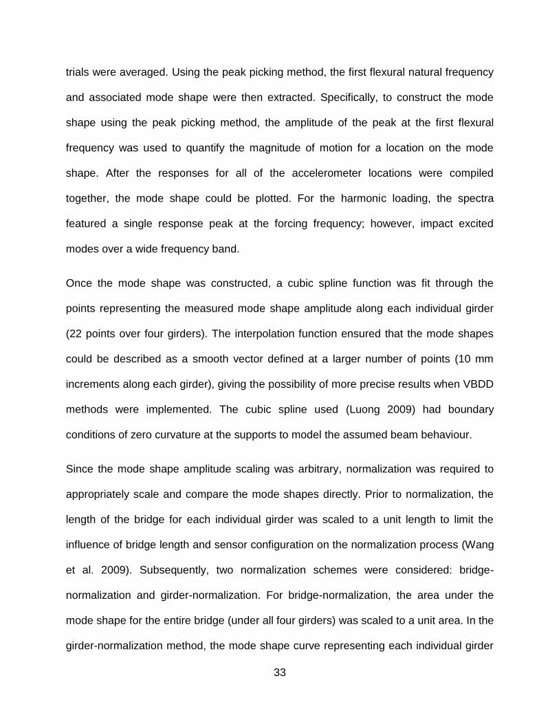
33

trials were averaged. Using the peak picking method, the first flexural natural frequency

and associated mode shape were then extracted. Specifically, to construct the mode

shape using the peak picking method, the amplitude of the peak at the first flexural

frequency was used to quantify the magnitude of motion for a location on the mode

shape. After the responses for all of the accelerometer locations were compiled

together, the mode shape could be plotted. For the harmonic loading, the spectra

featured a single response peak at the forcing frequency; however, impact excited

modes over a wide frequency band.

Once the mode shape was constructed, a cubic spline function was fit through the

points representing the measured mode shape amplitude along each individual girder

(22 points over four girders). The interpolation function ensured that the mode shapes

could be described as a smooth vector defined at a larger number of points (10 mm

increments along each girder), giving the possibility of more precise results when VBDD

methods were implemented. The cubic spline used (Luong 2009) had boundary

conditions of zero curvature at the supports to model the assumed beam behaviour.

Since the mode shape amplitude scaling was arbitrary, normalization was required to

appropriately scale and compare the mode shapes directly. Prior to normalization, the

length of the bridge for each individual girder was scaled to a unit length to limit the

influence of bridge length and sensor configuration on the normalization process (Wang

et al. 2009). Subsequently, two normalization schemes were considered: bridge-

normalization and girder-normalization. For bridge-normalization, the area under the

mode shape for the entire bridge (under all four girders) was scaled to a unit area. In the

girder-normalization method, the mode shape curve representing each individual girder

34

was scaled to enclose an area of unity. As such, the relative mode shape amplitudes

between girders were maintained in the bridge-normalized method, and lost in the

girder-normalized method. Further equations and figures describing the two

normalization schemes are presented in Section 4.2.3.

3.6. PRELIMINARY TESTS TO DEFINE TEST PROTOCOLS

3.6.1. Overview

This section briefly summarizes some of the preliminary testing that was done to

understand the bridge behaviour prior to undertaking the main experimental program.

Based on these findings, specific decisions were made regarding the testing conditions

for the remainder of the testing program. Specifically, this section covers issues related

to the energy transfer between the closely spaced lower modes.

3.6.2. Interference Between Lower Modes

Initial dynamic testing was applied considering an unloaded bridge and the hydraulic

shaker located over node #15 (Figure 3.5). These initial tests revealed that two lower

vibration modes were spaced very close together on the frequency spectrum (i.e., had

similar natural frequencies). This resulted in problems with exciting the first flexural

mode using either harmonic or impact excitation without also generating interference

from the first torsional mode. Instead of extracting pure mode shapes, peak picking

methods resulted in “operational deflection shapes” containing more than one mode,

with each having a different shape and phase angle (time lag). It should be noted that

the “operational deflection shapes” could be misinterpreted as actual mode shapes for

35

structures with closely spaced natural frequencies. In addition, typical impact tests with

excitation to the centre of the bridge resulted in initial excitations to the fundamental

frequency with subsequent energy transfer to the torsional modes (outer girders).

Figure 3.7 shows the two lower mode shapes, including the first flexural and first

torsional modes. These mode shapes were produced using impact loading on the

unloaded timber bridge deck; however, the hydraulic shaker was located at node #15.

Theoretically (and also in Figure 3.7), the first flexural mode shape should result in

girder motion that is synchronized (in-phase) and has similar amplitudes at

corresponding locations on all the girders. On the other hand, the first torsional mode

should result in differential movement across the girders, with the two halves of the

bridge being 180o out of phase with each other. In many of the preliminary tests, it was

found that it was difficult to discern between the two mode shapes, since the

frequencies were closely spaced, as shown on the spectrum in Figure 3.8.

Figure 3.7. Comparison of the first torsional and first flexural mode shapes of the bare

bridge

36


impact excitation, showing the closely spaced flexural and torsional modes

The closely spaced lower modes resulted in the extraction of apparent mode shapes

that were actually a combination of the first flexural and torsional modes. Since the

individual modes could not be adequately distinguished from each other (especially

using harmonic loading), the first flexural mode was selected as being of primary

importance. Steps were taken to suppress the effects of the first torsional mode, and

magnify those of the first flexural mode, as described in Section 3.6.3.

3.6.3. Methods for Accentuating the First Flexural Mode

Two methods were used to amplify the response of the first flexural mode. First, the

response of the first flexural mode was increased by exciting the bridge at its centre

while using the hydraulic shaker. Since the centre of the bridge was a theoretical nodal

point (point of zero displacement) for the first torsional mode, harmonic or impact

excitation applied at the centre of the bridge would not be effective in exciting torsional

motion. It should be noted that uniform weight was also added at this time (described in

37

Section 3.7.4) to model the effect of superimposed mass on the timber bridge, which

was unrelated to accentuating the first flexural mode.

The placement of the hydraulic shaker mass at the centre of the bridge, in turn, also

allowed for considerable energy transfer to the first torsional mode (alternatively, to the

outer girders). In other words, the addition of the shaker mass made it relatively easier

to excite the torsional mode since the flexural mode became more difficult to excite (the

shaker mass was placed at a location with considerable movement for the first flexural

mode). Consequently, additional mass was also added at mid-span of the outside

girders to replicate the effect of the shaker mass on the middle of the outer girders,

which further separated the natural frequencies by lowering the torsional natural

frequency. The resulting change in the frequency response spectrum is shown in Figure

3.9, where the bridge was now subjected to superimposed mass (a more in-depth

description of the mass on the bridge is provided in Section 3.7.4). Note the reduction of

torsional amplitude, in addition to the increased separation of the modes, shown in

Figure 3.9 as compared to Figure 3.8.

By amplifying the response of the first flexural mode relative to that of the lowest

torsional mode, there was a considerable decrease in the quality of the first torsional

mode shape results. Similar to “operational deflection shapes” described in Section

3.6.2, further attempts to plot the torsional mode shape resulted in anomalies in both the

girder amplitudes and phase angles, thus resulting in a torsional mode shape that could

not be used for further analysis. As a result, only the lowest flexural mode is considered

in subsequent analyses.

38


impact excitation after the torsional mode was suppressed

3.7. DAMAGE CASES CONSIDERED

3.7.1. Overview

The primary purpose of this study was to determine the effect of changes in

substructure stiffness on dynamic characteristics. As such, this section summarizes the

work that was done to determine realistic pile head stiffness values, taking into account

the soil-pile interaction. Upper and lower bounds on pile stiffness were considered,

along with various soil stiffness values, to obtain a realistic range of effective foundation

stiffness characteristics. Support conditions intended to reproduce this range of effective

foundation stiffness were then applied under the timber bridge in the laboratory to allow

for testing under a variety of substructure condition states.

39

In addition, it was of interest to determine the influence of superimposed mass (ballast)

distributed over the timber deck, as well as superstructure damage. These variables

and the cases considered are also presented in this section.

3.7.2. Determination of Substructure Stiffness

The effective substructure stiffness (keff) of a timber pile is a combination of the stiffness

of the pile above ground (pile stiffness, kp) arranged in series with the portion of pile

located below ground, having a soil-pile stiffness of ks. Equation 3.1 and Figure 3.10

show the field conditions that the supports used in the laboratory tests were intended to

model:

[3.1]

Figure 3.10. Effective stiffness model by considering the soil-pile interaction of an

embedded timber pile

40

The pile stiffness above ground can be estimated as the stiffness of an axially loaded

column, which can be expressed as

[3.2]

where L is the length of pile above ground, E is the modulus of elasticity of the timber

pile and A is the cross sectional area of the pile. However, Equation 3.2 assumes that a

pile acts as a linear material, which is not likely the case, as shown in Figure 3.11.

Timber, when exposed to the environment and service loads, is susceptible to

reductions in strength and stiffness due to fatigue, increased moisture content and

decay (Ritter 1990). For example, initial stiffness at low loads can decrease

considerably with increased moisture content (Martenson 2003). During vibration

testing, a bridge and its supporting piles are expected to be at low service loads,

meaning that the pile stiffness may be considerably lower than that described in

Equation 3.2 due to the increased timber flexibility caused by the variables listed above

(fatigue, increased moisture content and decay). As such, to determine pile stiffness

values at service level loading, data from a past study were used (Donovan 2004). In

this study, 33 creosote treated timber piles gathered from across the United States were

tested to failure and the load-deflection curves were tabulated. The researchers noted a

typical non-linear behaviour, where the pile stiffness at higher loadings, prior to failure,

was considerably higher than the service load stiffness, which is conceptually shown in

Figure 3.11.

41

Figure 3.11 Typical applied load vs. average axial deflection behaviour for a timber pile

with highlighted low and high load pile stiffness (after Donovan 2004)

A summary of the pile stiffness ranges are shown in Figure 3.12, where the x-axis

represents the pile stiffness at high loadings (when a linear load-deflection curve is

reached) and the y-axis represents the pile stiffness at a lower load (when the pile still

behaves as a non-linear material). Note that the service level stiffness is approximately

0.22 that of the linear region at higher loadings, as indicated by the line of best fit

through the data (the linear fit was set to have an intercept of zero). Figure 3.12 also

provides upper and lower boundaries for expected above ground pile stiffness for piles

in the field. A range of 20-90 kN/mm was selected to model realistic above ground pile

stiffness in the field.

42

Figure 3.12. Low load pile stiffness vs. high load pile stiffness, showing a range of

above ground pile stiffness, kp (data from Donavan 2004)

To determine the deformation of a pile for the portion located below the ground, a

method by Poulos and Davis (1980) was used, as outlined by Fleming et al. (2009).

There are three types of settlement that were considered: (1) the base settlement, (2)

the shaft settlement, and (3) pile compression. However, for service level loading, the

shaft settlement governs, which is mainly a function of the modulus of rigidity of the soil.

The stiffness of the pile-soil system below ground can then be solely attributed to shaft

settlement and can be described as

[3.3]

43

where Ls is the length of pile extending below ground, G is the shear modulus of the

soil, and ζ describes the measure of radius of influence of pile (a function of the length

of pile below ground and pile diameter, ζ ≈ ln[2Ls/d]).

Considering Equation 3.3, common values for pile dimensions below ground, and a

range of common soil elastic moduli (U.S Army Corps of Engineers 1990), the soil-pile

system stiffness range is shown in Figure 3.13 (30-160 kN/mm). Note that the

relationship between shear modulus and modulus of elasticity is

.

Figure 3.13. Range of soil-pile system stiffness below ground, ks

Using the ranges of soil-pile system stiffness below ground (ks), the above ground pile

stiffness values (kp) that were selected, and considering springs in series (Equation 3.1),

44

an effective stiffness for the soil-pile system could then be calculated. The results are

shown in Table 3.3.

Table 3.3. Foundation stiffness window (per pile)

Hard (kN/mm)

Soft (kN/mm)

ks 160 30

kp 90 20

keff 58 12

Once the upper and lower stiffness bounds were calculated, the range had to be

implemented on the timber bridge substructure in the lab. The substructure setup used

in the lab is shown in Figure 3.14. This figure illustrates how wood blocking was used to

achieve the desired stiffness values. A steel block was fastened to the underside of the

pile cap to uniform bearing for all condition states. Pine and oak blocks were then

placed underneath the steel blocks to represent different substructure condition states.

Figure 3.14. Wood block support setup (front and side views)

45

To ensure the effective stiffness values of the modelled supports were compatible with

those shown in Table 3.3, stiffness testing was done on the wood block supports. Each

pile was modelled as two wood blocks placed side by side, each with dimensions of

50_mm x 50_mm x 150_mm. Using a Universal Testing Machine (Instron 600DX), two

wood blocks were compressed to a load of 5 kN with a loading rate of 5 kN/min. The

test setup is shown in Figure 3.15. The wood blocks were sandwiched between two

steel blocks to simulate their configuration under the pile cap in the laboratory. Two dial

gauges were placed, one on either side of the specimen, to measure the small

displacements (precision of ±0.0025 mm or 0.0001 in) and to ensure uniform distribution

of the load.

Figure 3.15. Test setup to determine support stiffness

The load deflection curve was plotted using the load gauge (read to a precision of

±4.45_N) from the Universal Testing Machine and the deflection gathered with dial

gauges. Readings were taken every 0.013 mm (0.0005 in) for the oak block tests, and

46

every 0.051 mm (0.002 in) for the pine tests. Each oak block and pine block

configuration was repeated for three trials (each with different wood blocks), and the

data points are plotted in Figure 3.16. A line of best fit was then applied to each test

(using least squares and intercept of zero) to attain an overall stiffness for each trial.

The stiffness values (slopes) produced for similar block cases were then averaged and

are plotted in Figure 3.16, where the slope represents the stiffness of the block system.

Also, a confidence interval (α=0.1) was calculated using the average and standard

deviation of the slopes/stiffness from the three tests. It can be seen that the pine

foundation closely models the “soft” foundation, and the oak models the “hard”, as

presented in Table 3.3.

Figure 3.16. Pine and oak block foundation load deflection curve (per support)

47

Refer to Appendix B for more details on the calculations and data used to complete this

section.

3.7.3. Substructure Damage Cases

A summary of the substructure condition states can be seen in Table 3.4.

Table 3.4. Substructure condition states Condition State Graphic Description

D0

Rigid-Rigid Both ends of the bridge were supported by four sets of steel blocks.

D1

Hard-Rigid The left support was “hard” (four sets of oak blocks) and the right support was rigid.

D2

Soft-Rigid The left support was “soft” (four sets of pine blocks) and the right support was rigid.

D3

Non-Uniform-Rigid The left support was “soft” under Girders 3 and 4 (two sets of pine blocks) and rigid under Girders 1 and 2 (two sets of steel blocks), while the right support was rigid.

D4

Soft- Soft Both sides of the bridge were uniform “soft” supports (four sets of pine blocks under each pile cap).

D5

Hard- Hard Both sides of the bridge were uniform “hard” supports (four sets of oak blocks under each pile cap).

D6

Soft- Hard The left support was “soft” (four sets of pine blocks) and the right support was “hard” (four sets of oak blocks).

A “rigid” case was used as the base case, and exhibited a stiffness exceeding that

which would be expected in the field. The “hard” foundation case represented the

stiffness of a healthy pile in stiff soil, and the “soft” foundation case represented a

deteriorating pile in soft soil. In all condition states, with the exception of D3, the

48

foundation had a uniform stiffness under either pile cap, meaning that each of the four

supports under a pile cap were similar. There were a large number of foundation cases

that could have been examined; however, the six foundation cases shown in Table 3.4

represent the scope of this study.

3.7.4. Weight Cases

The mass of a system can influence the dynamic response significantly. The weight

cases considered in this study were meant to take into account the variability in the

weight of the wearing surfaces that would occur in the field. The bare timber bridge in

the laboratory had a total mass of 1630 kg, which corresponded to a uniform dead load

of 1.11 kPa distributed over the surface area. To determine the mass of the timber

bridge, the density was first calculated by weighing a 0.227 m3 potion of the bridge

(having a mass of 116 kg). The total mass of the bridge was then extrapolated using the

calculated density of 510 kg/m3 and an approximate volume of 3.2 m3 (not including the

pile caps).

To increase the weight of the bridge to account for a percentage of the wearing surface

that would be present in the field, concrete blocks were placed on the deck surface. The

blocks were approximately uniformly distributed; however, additional blocks were placed

at the centre of the outer girders (Girders 1 and 4) for reasons described in Section

3.6.3. The distribution of the blocks and the two weight cases considered can be seen in

Figure 3.17. Weight Case 1 (W1) provided an additional load of 0.27 kPa over the bare

timber bridge deck. To attain Weight Case 2 (W2), a single concrete half block was

placed on top of each of the concrete blocks shown in Figure 3.17. Weight Case 2

49

resulted in an additional 0.41 kPa over the bare timber bridge deck. The two weight

cases presented were not intended to represent realistic weights that would be seen in

the field, but it is possible that they reduced the effects of non-linear behaviour by pre-

loading the structure. Furthermore, to realistically model the mass of a wearing surface

that would be present in the field, significantly more blocks would be required, which

would have introduced significant tripping hazards to the bridge surface.

Figure 3.17. Plan view of the deck, showing the distribution of concrete blocks used to

produce the two weight cases

Figure 3.18 shows the timber bridge in the laboratory loaded to Weight Case 1. The

additional blocks over the outer girders can be seen clearly. These blocks were placed

to offset the effects of the weight of the hydraulic shaker at the centre of the bridge,

thereby suppressing the effects of the first torsional mode and accentuating a response

at the first flexural mode shape (described in Section 3.6.3).

50

Figure 3.18. Timber bridge loaded with Weight Case 1 (W1)

A summary of the weight cases is provided in Table 3.5.

Table 3.5. Summary of the weight cases considered Condition state Graphic Description

W1

Weight Case 1 Represents ~10 mm gravel wearing surface. The mid-span of the two outside girders was more heavily loaded to separate the first torsional and flexural mode.

W2

Weight Case 2 Represents ~15 mm gravel wearing surface. The mid-span of the two outside girders was more heavily loaded to separate the first torsional and flexural mode.

3.7.5. Superstructure Damage Cases

Superstructure damage cases were limited to reductions in flexural rigidity. A skill saw

was used to make a 60 mm deep cut on the bottom of Girder 2 (Damage Case S1) and

subsequently to Girder 4 (Damage Case S2). These condition states are shown in

Table 3.6.

51

Table 3.6. Superstructure condition states Condition state Graphic Description

S0

Baseline Condition This was the base case for the timber bridge in the laboratory.

S1

Flexural cut beneath Girder 2 60 mm deep cut beneath Girder 2 at mid span (2700 mm from the left support). The cut was made with a skill saw and reduced the girder moment of inertia to 62% of the original (not considering composite action with the deck).

S2

Flexural cut beneath Girder 4 60 mm deep cut beneath Girder 4 at 1/3 the span (1890 mm from the left support). The cut was made with a skill saw and reduced the girder moment of inertia to 62% of the original (not considering composite action with the deck). This cut was made after S1

3.8. SUMMARY OF THE EXPERIMENTAL PROGRAM

3.8.1. Overview

This section summarizes the specific damage states and tests that were completed for

this experimental program. This includes the different combinations that were examined

using two excitation sources and various condition states. A summary of the bridge

setups that were tested is shown in graphic format in Figure 3.19, which presents the

graphics and the text notation used to represent different bridge configurations and

excitation sources that are used for the remainder of the thesis. The bridge state

D0S0W1 represents an undamaged lightly loaded bridge on rigid supports, and was

used as a baseline for comparison to all other damage states. In the notation adopted

for this study, the first two characters (D0 to D6) denote the support condition state, the

second two characters (S0 to S2) denote the superstructure condition state, and the

final two characters (W1 to W2) denote the super-imposed mass on the timber bridge

52

deck. All tests were run using both harmonic loading and impact loading, using the

average of five repeated tests.

Figure 3.19. Summary of experimental program

53

3.8.2. Substructure Damage Program

The substructure damage program was completed to investigate the influence of the

substructure stiffness alone on the dynamic response of the bridge. This phase

consisted of four test setups, D0S1W1a, D1S0W1, D2S0W1, and D3S0W1. The

subscript „a‟ signifies that this test setup was subsequently used again, but the supports

were changed for other testing in-between.

3.8.3. Weight Case program

The weight case program considered changes to the weight on the timber bridge in

conjunction with changes to the substructure stiffness. This was conducted to uncover

the influence the super-imposed mass had on the dynamic response. This phase

consisted of four bridge arrangements, D0S0W1b, D0S0W2, D4S0W1a, and D4S0W2.

Note that base case, D0S0W1, had to be re-established to carry out this phase

(signified by the subscript „b‟).

3.8.4. Substructure and Superstructure Interaction Program

The final testing program was conducted to determine the effects of superstructure

damage alone on the timber bridge response. Additionally, the interaction of

superstructure damage with substructure damage to both supports was of interest. The

testing program considered many damage states, which consisted of D0S0W1c,

D4S0W1b, D5S0W1, D6S0W1, D0S1W1, D4S1W1, D5S1W1, D6S1W1, D0S2W1,

D4S2W1, D5S2W1, and D6S2W1. The process for testing was to cycle through

substructure states, then to introduce superstructure damage, and then re-establish the

dynamic properties considering all substructure states again.

54

4. TIMBER BRIDGE DAMAGE DECTECTION RESULTS

4.1. INTRODUCTION

This chapter presents the results of the timber bridge damage detection program

described in Chapter 3. Forms of damage investigated included both substructure and

superstructure damage. As well, the influence of superimposed weight added on top of

the bridge deck was considered to investigate possible nonlinear effects associated with

the closing of cracks in the timber. Changes in dynamic response were studied primarily

using comparisons of the first flexural mode shape, but changes in the fundamental

natural frequency were also considered.

The primary objective of this study was to investigate the feasibility of detecting realistic

changes in substructure stiffness using vibration-based methods, in addition to studying

the interaction between the substructure and superstructure responses.

4.2. BRIDGE BEHAVIOUR

4.2.1. Overview

The overall bridge response to dynamic excitation is presented in this section.

Characteristics of the first flexural mode are presented in the most detail, including its

associated natural frequency and mode shape.

55

The data gathered using both harmonic and impact excitation methods are presented,

and the advantages and disadvantages of both methods are considered. In addition, the

two methods for normalizing the measured mode shape are compared and contrasted.

4.2.2. Dynamic Response

The modes that were most easily excited on the timber bridge were the lower modes,

which included the first flexural and torsional modes. Figure 4.1 presents the

acceleration spectrum produced by the reference accelerometer due to impact loading;

here, the greatest spectral amplitude for the reference accelerometer has been scaled

to unity. The bridge configuration for the data presented in Figure 4.1 was the initial

bridge state after the steps were taken to separate the lower modes, as presented in

Section 3.6.3. The first flexural mode was of particular interest for this study because of

the ease with which it could be excited and the fact that the lowest mode has been

proven in past studies to provide the most reliable indications of damage (Zhou 2006;

Wang et al. 2009).

Figure 4.1. Frequency spectrum of the reference accelerometer for foundation case

D0S0W1a using impact loading

56

Figure 4.2 presents the first flexural mode shape for the base condition state

(D0S0W1a) produced with impact loading. The mode shape has been bridge-

normalized (see Equation 2.4 and Section 3.5.3), so the relative amplitudes of different

girders could be preserved.

Figure 4.2. First flexural mode shape for foundation case D0S0W1a, obtained using

impact loading

The left support was then changed from rigid to the hard foundation case (D1S0W1);

the mode shape for this case is presented in Figure 4.3. Again, the mode shape was

bridge-normalized and was produced using impact excitation. It is important to note that,

for the stiffer foundation cases presented in Figure 4.2 and Figure 4.3, the amplitude of

girder movement across the bridge deck remained relatively constant.

Upon changing the left support to a “soft” condition, there was a definite change in the

first flexural mode shape produced, as seen in Figure 4.4. A difference in the relative

girder movement across the bridge is observed when the more flexible substructure was

introduced. Girder 4 was found to have the largest deflections, with deflections

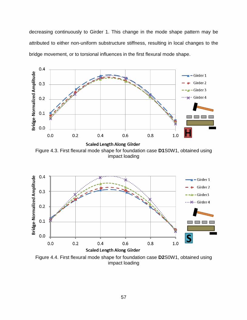
57

decreasing continuously to Girder 1. This change in the mode shape pattern may be

attributed to either non-uniform substructure stiffness, resulting in local changes to the

bridge movement, or to torsional influences in the first flexural mode shape.


impact loading


impact loading

58

The bridge behaviour that is seen Figure 4.4 is similar to the mode shapes that were

produced in the preliminary work presented in Section 3.6.2 before measures were

taken to separate the lowest flexural and torsional modes. Figure 4.5 shows the

frequency spectrum over the frequency range covering the lowest two modes for the

foundation cases presented in the above figures (D0S0W1a, D1S0W1, and D2S0W1). It

can be seen that, as the timber bridge substructure was incrementally softened, the

separation between the lower modes became smaller. As such, the interaction between

the two modes became greater, and the first flexural mode increasingly began to

resemble the torsional mode, as seen in Figure 4.4.

Figure 4.5. Acceleration spectra showing the first flexural and torsional natural

frequencies under different damage states

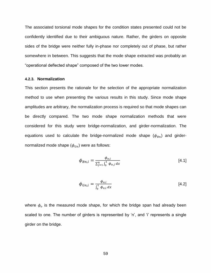
59

The associated torsional mode shapes for the condition states presented could not be

confidently identified due to their ambiguous nature. Rather, the girders on opposite

sides of the bridge were neither fully in-phase nor completely out of phase, but rather

somewhere in between. This suggests that the mode shape extracted was probably an

“operational deflected shape” composed of the two lower modes.

4.2.3. Normalization

This section presents the rationale for the selection of the appropriate normalization

method to use when presenting the various results in this study. Since mode shape

amplitudes are arbitrary, the normalization process is required so that mode shapes can

be directly compared. The two mode shape normalization methods that were

considered for this study were bridge-normalization, and girder-normalization. The

equations used to calculate the bridge-normalized mode shape ( ) and girder-

normalized mode shape ( ) were as follows:

[4.1]

[4.2]

where is the measured mode shape, for which the bridge span had already been

scaled to one. The number of girders is represented by „n‟, and „i‟ represents a single

girder on the bridge.

60

The bridge-normalization method produces a mode shape that encloses a unit-area

under the entire bridge, while a girder-normalized mode shape encloses a unit-area

under each individual girder. Furthermore, all girders in the bridge-normalization

scheme have the same scaling factor, while each is different under girder-normalization,

as shown in Equations 4.1 and 4.2.

Figure 4.6 illustrates the influence of the normalization scheme on a mode shape

generated using pseudo data, which was fabricated to show the effects of

normalization. It is clear that the bridge-normalization scheme maintains the relative

girder amplitudes for the mode shape, so that each girder encloses a different area. The

girder-normalization scheme, however, scales each individual girder to enclose an area

of unity.

All figures presented in this chapter thus far were generated using the bridge-

normalization method, where the relative girder amplitudes have been maintained to

represent the actual motion of the bridge (see Figure 4.6a). To compare the two

normalization schemes using measured data, Figure 4.7 presents the bridge-normalized

mode shape for the soft foundation case (which is the same case as that plotted in

Figure 4.4, but achieved through harmonic loading), while Figure 4.8 presents the same

mode shape but generated using girder-normalization.

61

Figure 4.6. Representations of the same mode shape using the (a) bridge- and (b)

girder-normalization schemes (generated using pseudo data)

62

Figure 4.7. Bridge-normalized representation of the soft foundation case (D2S0W1)

Figure 4.8. Girder-normalized representation of the soft foundation case (D2S0W1)

The girder-normalization method seems to attenuate the influence of torsional

behaviour in the first flexural mode shape by scaling each individual girder mode shape

to encompass a unit-area, thereby forcing the peak mode shape amplitude along each

girder to be roughly equal and allowing for a more direct comparison between girders.

Since this study focused on relative movements between the substructure and

superstructure, rather than relative movement between girders, the girder-normalization

63

method was implemented for the remainder of the study. Consequently, the girder-

normalization scheme also attenuated the influence of torsional behaviour.

4.2.4. Mode Shape Variability

The primary method of vibration-based damage detection used in this study was the

comparison of the first flexural mode shapes for the bridge in different conditions.

Damage was inferred using changes in the mode shape. Typically, small-scale damage

results in minor changes to the mode shape. Consequently, the mode shapes need to

be known to a high degree of certainty. Figure 4.9 shows the variability of the measured

mode shape gathered by harmonic loading for the base case (D0S0W1a). For this case,

the resulting average coefficient of variation in mode shape amplitudes at various

sensor locations was approximately 0.07% based on five repeated trials. This high

degree of precision was found to be sufficient to enable the detection of small-scale

damage.

The results for impact loading are shown in Figure 4.10. Here, there was considerably

more variability, with an average coefficient of variation of approximately 0.69% in the

mode shape amplitudes. As a result, it was more difficult to detect small-scale damage

using impact loading due to the increased noise in the mode shape. However, impact

loading is still considered to be of practical interest due to its ease of implementation in

the field.

64


harmonic excitation


impact excitation

Similarly, the natural frequencies produced using harmonic loading were found to a

higher degree of certainty. In this study, the natural frequencies produced through

harmonic loading were measured to a precision of ±0.05 Hz, while those measured

using impact loading had lower precision at ±0.12 Hz.

65

4.2.5. Mode Shape Components

The mode shape of the bridge superstructure, supported on flexible supports, was

broken down into the following three components, illustrated in Figures 4.11 to 4.13, to

describe the bridge‟s response to vibration:

A. Flexural response: The flexural component (A) describes the area of the mode

shape remaining once the substructure motion (components B and C) has been

removed. This component corresponds to the movement of the superstructure

when excited at its first flexural natural frequency.

B. Differential support movement: This component accounts for the portion of the

substructure movement resulting from differential support stiffness. The

contribution of this component can be described by the triangular area (B)

representing the difference in support movement at the two ends of the girder.

This component was defined as positive for cases where the left support had a

greater amplitude and negative when the right support had a greater amplitude to

ensure that the differential support movement was completely quantified with the

differential component.

C. Uniform support movement: This component is defined by the smaller of the two

mode shape amplitudes at either end of the girder (i.e., over the supports).

Represented by area C, the uniform support movement may be caused either by

the compressibility of the timber pile cap or by flexibility in the foundation below

the cap.

The girder-normalized first flexural mode shape for the base case (Girder 1) is shown in

Figure 4.11. The mode shape has been decomposed to separate the mode shape into

66

the three components. Similarly, Figure 4.12 and Figure 4.13 show the corresponding

mode shape components for foundation cases with an incrementally softened left

support. As the left support was incrementally softened, a definite change in the mode

shape geometry may be noted. All figures were produced with harmonic excitation;

however, impact loading gave similar results.


excitation), subdivided into its three components



67



The mode shapes have been girder-normalized for the above figures and the remainder

of the analysis for this study, unless otherwise noted. The girder-normalization ensured

a unit-area under each girder, suggesting that the area under three components add to

unity. In addition, the girder-normalization method allowed the contribution of each

component for individual girders to be directly compared without regard to amplitude.

Figure 4.11 presents the mode shape of Girder 1 for the stiffest support case (base

case); the mode shape is largely dominated by flexural deformations (A). Nevertheless,

there is still considerable uniform support movement, C, which can be attributed to

compression within the pile caps and the girder directly above the caps. As the left

support is incrementally softened from Figure 4.11 to Figure 4.12 to Figure 4.13 it is

apparent that the differential support movement, B, becomes relatively more prominent.

This suggests that a simple observation of the relative contributions of the mode shape

components can provide valuable insight into the condition of the substructure.

68

4.2.6. Summary

The bridge behaviour was governed by the first flexural mode shape; however, since

the natural frequency of the torsional mode was close to that of the flexural mode there

was some energy transfer to the torsional mode, resulting in difficulties extracting pure

mode shapes. Steps were taken to force the response to occur at the first flexural mode

by exciting the bridge at the centre and by distributing weight on the bridge surface to

suppress the torsional mode.

The girder-normalization method was used exclusively for the analysis of the mode

shapes for this study since it allowed for direct comparison of the mode shape

components for different girders. The mode shape was deconstructed into two basic

types of deformations; substructure and superstructure. The superstructure component

exclusively comprised of flexural deformations, while the substructure components were

described by differential and uniform support movement.

4.3. DETECTION OF SUBSTRUCTURE DAMAGE TO A SINGLE SUPPORT

4.3.1. Overview

This section presents the results for the substructure condition states featuring damage

to the left support only. Foundation cases considered were the rigid base case (D0), the

“hard” (D1) and the “soft” (D2) cases, in addition to a non-uniform soft case (D3).

Damage was inferred using the deconstructed mode shape in conjunction with both a

simple observation and a quantitative comparison of the areas enclosed by each

component.

69

The relative efficiency of both impact and harmonic excitation methods were compared

based on their success in inferring damage. Also, the natural frequency changes

resulting from increasingly soft foundation cases were considered to investigate their

potential contribution in VBDD methods.

4.3.2. Uniform Substructure Deterioration

This section discusses the same foundation cases as Section 4.2.5, but considers the

mode shapes along all four girders. The foundation cases considered are the rigid case

(D0S0W1a), the hard foundation case (D1S0W1) and the soft foundation case

(D2S0W1). All of the condition states had a right support that was rigid, while the left

support was uniformly and incrementally softened.

The deconstructed girder-normalized mode shapes for all girders are shown in Figures

4.14, 4.15 and 4.16. All data for these figures were gathered using harmonic loading;

however, impact loading yielded similar results. All the mode shapes gathered for this

study are presented in Appendix C (based on the average of five repeated trials as

presented in Chapter 3).

Figure 4.14 presents the results for the rigid support case, for which the fundamental

flexural mode shapes along of all the girders have been deconstructed into the three

components described in Section 4.2.5. The mode shape along each individual girder

encloses an area of unity. Upon inspection of the mode shape along each individual

girder, it is apparent that the flexural deformations (component A) account for a large

portion of the movement. Again, there is also considerable uniform foundation

movement (component C), with very little differential support movement (component B),

70

similar to Figure 4.11. There are, however, differences in the mode shape components

among the girders, despite the fact that this represented a case featuring uniform

support stiffness across the bridge width (also shown in the bridge-normalized mode

shapes shown in Figures 4.2, 4.3, and 4.4). The differences across the girders are most

apparent in the amount of uniform support movement, C, observed in each case. The

same conclusion can also be drawn when observing the mode shapes for the other

condition states, shown in Figure 4.15 and Figure 4.16. Differences in the mode shape

component amplitudes across the bridge may be due to variations in the stiffness of the

substructure or superstructure; however, there may also still be some torsional

interference involved. Additionally, the differences in the mode shape amplitudes among

girders could not confidently be described by the condition of the girders or pile caps.

As the foundation was incrementally softened relative to the base case, there was

increasingly more differential foundation movement (B) in the girders (shown in Figure

4.15 and Figure 4.16). Stiffness changes to the substructure could therefore be inferred

simply by comparing the relative amplitudes of the mode shape components in the

figures. This suggests that the mode shape component method requires a comparison

of response from other bridge states to the relative “health” of the substructure.

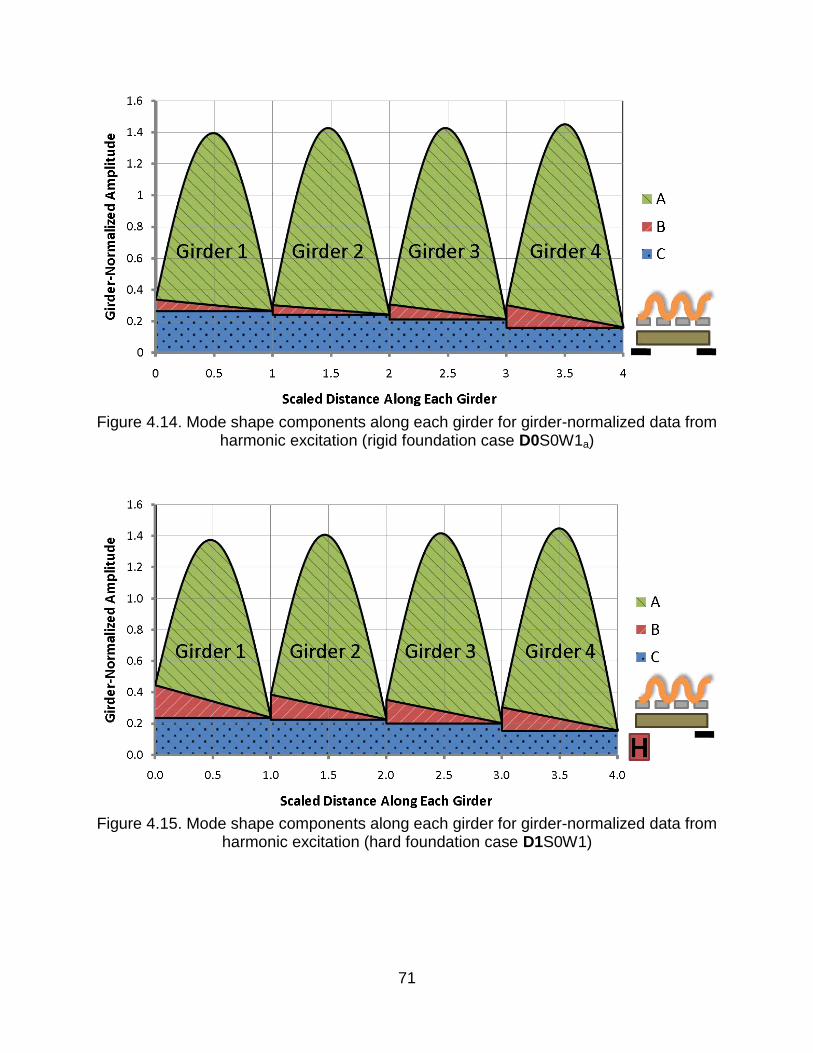
71


harmonic excitation (rigid foundation case D0S0W1a)


harmonic excitation (hard foundation case D1S0W1)

72


harmonic excitation (soft foundation case D2S0W1)

4.3.3. Local Substructure Deterioration

The only foundation case featuring non-uniform local substructure damage had the left

end of Girders 3 and 4 bearing on a soft support, while the other supports remained

rigid. The frequency spectrum of the lower modes can be seen in Figure 4.17. Although

the first flexural and torsional modes are closely spaced, there is a separation valley

between the response peaks, making it possible to clearly identify the modes.

When the mode shape was girder-normalized and deconstructed into the three mode

shape components, as shown in Figure 4.18, a large difference in the relative

responses along the four girder lines is apparent. Considerable differential support

movement (B) was observed under the soft supports (Girders 3 and 4), whereas this

movement under Girders 1 and 2 was much less.

73

Figure 4.17. Partial frequency spectrum for the reference accelerometer for foundation

case D3S0W1, showing the first torsional and flexural natural frequency separation


excitation (D3)

It should be noted that the relative girder movement for the local substructure case,

shown in Figure 4.18, is distorted from the actual bridge movement that would have

been apparent using the bridge-normalization scheme. Figure 4.19 shows the bridge-

normalized mode shape, where the actual relative girder movements are presented.

74

The girders above the soft supports (Girders 3 and 4) exhibited relatively little motion,

when compared to the girders over the rigid supports. This is likely due to the fact that

the energy over the softened supports was dissipated by compressing the foundation,

rather than bending the relatively stiff superstructure.

Figure 4.19. Mode shape components for bridge-normalized data from harmonic

excitation (D3)

4.3.4. Quantitative Analysis with Mode Shape Components

Up to this point, substructure damage detection has been accomplished by a simple

visual comparison of the mode shape components. A more thorough method for direct

comparison is to evaluate the amplitudes of areas enclosed by the mode shape

components, to allow for a quantitative analysis. A summary of the mode shape

components for multiple bridge condition states is shown in Appendix D.

The remainder of the study makes use of a standard chart to summarize the mode

shape data produced through deconstructing mode shapes. A labelled summary of a

75

chart is shown in Figure 4.20 (produced using the same pseudo mode shapes

presented in Figure 4.6). In the figure, and all that follow it, the mode shape components

for individual girders are plotted separately. In addition, the averaged mode shape

components over all four girders are plotted, and the standard deviations of the

components are illustrated using horizontal error bars. Figure 4.20 also has an

embedded table showing specific values for each mode shape component for reference

purposes.

Figure 4.20. Illustration of the standard chart used to summarize the mode shape

component data (produced using pseudo data)

Similar to Figure 4.20, Figure 4.21 presents a bar chart that summarizes the mode

shape component analysis for the foundation cases already considered (D0, D1, D2,

and D3). Once again, the relative differential support movement (B) is seen to

76

continuously increase as the left support was increasingly softened, while the uniform

foundation movement (C) stayed relatively constant. Consequently, the relative

contribution of the flexural deformations, A, decreased with continued softening,

suggesting that a healthy bridge state will feature significant flexural deformations, and

exhibit less substructure movement. Once again, it may be that the mode shape

components from other similar bridges with known condition states are required for a

comparative analysis to interpret specific patterns in the bridge response.

A further Student‟s t-test analysis (provided in Appendix G) confirmed the statistical

significance (α=0.1) of the variations in the differential support movement as the left

support was incrementally softened.

Figure 4.21. Mode shape components of girder-normalized data from harmonic loading

(D0, D1, D2, & D3)

77

Based on the error bars, it is evident that relatively large variations are present among

mode shape components along the four girders; this degree of variation was typical of

all tests. Consequently, it was concluded that results were best interpreted using

averaged mode shape components considering all girders. However, for the non-

uniform support case, D3, the between-girder variations in the mode shape components

were considerably larger. This suggests that such large variations could be indicative of

local damage that should be looked at more closely. A further statistical analysis is

presented in Appendix G that uses an F-test on variance to verify that the variance

present in the differential support movement on the non-uniform damage case (D3) was

statistically significant in relation to the uniform damage cases.

4.3.5. Effect of Excitation

Due to the ease of implementation, damage detection using impact applied to the

structure is likely the most efficient excitation method for field application. In this way,

VBDD could be made more practical by avoiding the need for using a hydraulic shaker

to assess damage. In this section, the mode shapes associated with various

substructure condition states are re-analyzed using data obtained when a hammer

strike was used as the excitation source.

Figure 4.22 is similar to Figure 4.21, but is plotted to feature data obtained through

impact loading. Similar to the results discussed in Section 4.3.4 (and Figure 4.21), the

data produced using impact loading suggests that changes in the substructure stiffness

may be inferred based on an observation of the deconstructed mode shape. As the left

support was incrementally softened, the relative differential support movement became

increasingly more prevalent. Likewise, the relative contribution of flexural deformations

78

decreased as the bridge state deteriorated. Also, the local substructure damage in state

D3 was evident in the large standard deviation given by differential substructure

movement component across the four girders, indicating that the individual girder

conditions differed.

Figure 4.22. Mode shape components for girder-normalized data from impact excitation

(D0, D1, D2, D3)

To implement impact testing in the field, no other form of excitation would be needed.

Although the test results in this study indicated that the hydraulic shaker achieved less

variable results (presented is Section 4.2.4), the mode shapes attained through impact

loading were capable of inferring the types of damage considered for this study. Table

4.1 presents the change in mode shape components from the base case (D0S0W1a) for

three condition states, considering both impact and harmonic loading. The base case is

compared with two foundation cases that were incrementally more flexible on the left

79

support (D1 and D2), in addition to a repeated trial of the base case (D0S0W1b), which

provides a means for assessing changes due solely due to repeated test setups. The

change in differential support movement (∆B) was higher for the tests conducted with

harmonic loading, suggesting that harmonic loading may be able to detect smaller

changes in the substructure stiffness. Harmonic loading resulted in a change in

differential substructure response that was, on average, 14.2% more compared to the

values produced using impact loading. However, impact loading did produce significant

changes with changing substructure stiffness.

Further comparisons of the two excitation methods are presented in Appendix G using

the Student‟s t-test.

Table 4.1. Change in mode shape components relative to the base foundation case (D0S0W1a) for multiple foundation cases, using two excitation methods

Harmonic

D0S0W1a

Change in mode shape component

∆A ∆B ∆C

Impact

D0S0W1a


∆A ∆B ∆C

D0S0W1b

-0.008 -0.017 0.003

D0S0W1b

0.000 -0.016 0.011

D1S0W1

-0.022 0.037* -0.015

D1S0W1

-0.017 0.032* -0.015

D2S0W1

-0.079* 0.106* -0.027

D2S0W1

-0.068* 0.094* -0.025

*Change is statistically significant (α=0.1)

80

4.3.6. Natural Frequency

Comparisons of natural frequencies can play an important role in VBDD methods. Mode

shape analysis alone will limit analysis to bridge deflections, where the stiffness of

superstructure can only be inferred in relation to the substructure (and vice versa).

However, including natural frequencies in the analysis may provide a means to assess

an approximate absolute stiffness of the entire structure, with which the relative stiffness

obtained from mode shape analysis may be of more value. Equation 2.7 gave a

relationship of natural frequency, bridge length, and bridge weight to the stiffness of the

bridge; such a relationship (or Equation 2.8) may provide an approximation of a bridge‟s

overall stiffness (Brashaw et al. 2008; Samali et al. 2003). Specifically, such interactions

may be used to assess the serviceability limit state, assuming the superstructure

stiffness (EI) can be calculated with some degree of confidence. A limitation of this type

of method is that it does not consider the effect that substructure flexibility has on the

global stiffness of a bridge.

Superstructure flexibility and substructure softness interact to reduce the natural

frequency. Mode shape components will only reveal relative stiffness; natural frequency

may be an indicator of the absolute stiffness of the entire structure. In this way, the first

flexural frequencies could be compared with that of other bridges (considering bridge

weight and length) as an indication of whether the bridge system meets serviceability

limit states requirements. Methods utilizing the natural frequency, possibly including a

relationship similar to Equation 2.7, could be implemented in the field to complement the

mode shape analysis.

81

The natural frequencies of the bridge structure for the foundation cases already

considered are listed in Table 4.2. The natural frequencies were obtained using

harmonic loading, in addition to impact loading. In general, the natural frequencies

obtained using impact loading were greater than that for harmonic, despite the bridge

configurations being equal in both tests (i.e., the mass from the shaker was present

during both excitation methods). Thus, it would appear that the timber bridge is stiffer in

the impact tests, which would suggest that different excitation methods and amplitudes

could introduce some non-linear behaviour. However, it is also likely that the observed

differences in natural frequency were due mainly to the precision with which they could

be measured using harmonic loading (using a sine sweep, as described in Section

3.5.2) as compared to impact loading (0.05 Hz versus 0.12 Hz).

Table 4.2. Fundamental frequency of the bridge for different softening cases under a single support.

Condition State

Natural frequency (Hz)

Harmonic Impact

±0.05Hz ±0.12Hz

D0S0W1a

15.91 15.99

D1S0W1

15.82 15.99

D2S0W1

15.33 15.50

D3S0W1

15.65 15.87

The trends observed in the first flexural natural frequencies for the various condition

states were as expected. The natural frequency was found to be higher for a stiffer

82

substructure condition state, and lower for a softer substructure. The natural

frequencies for all bridge condition states are shown in Appendix E.

4.3.7. Summary

This section introduced a method to infer substructure damage by deconstructing the

first flexural mode shape into components. Bridge condition states with various

substructure stiffness values were considered to understand specific mode shape

patterns related to substructure damage. Changes in substructure stiffness could be

detected using an observation of a single vibration test without reference to a baseline.

However, mode shape components from other known bridge states were required for a

comparative analysis to interpret specific patterns. Uniform damage to a single support,

in addition to a simple local damage case, all provided results that indicated the

presence of damage. Harmonic and impact loading gave similar results; however, the

results produced with harmonic loading did appear to be slightly more conclusive.

Changes in the first natural frequency were also analyzed. The observed changes in the

natural frequency were as expected; stiffer substructure cases had the highest natural

frequencies, and more flexible cases had incrementally smaller frequencies.

4.4. SUBSTRUCTURE DAMAGE DETECTION ON BOTH SUPPORTS

4.4.1. Overview

This section extends the work from Section 4.3 to include realistic substructure stiffness

conditions under both pile caps. A rigid support case was also included to act as a base

case.

83

4.4.2. Results and Discussion

The results for tests considering stiffness changes to both supports are shown in Figure

4.23 (produced using harmonic loading). The figure shows distinct patterns in the mode

shape components for specific damage states. It can be seen that the flexural

component (A) was relatively greater for stiffer supports, and the relative differential

support movement (B) was at a maximum for the differential (soft-hard) support case

(D6). The uniform support component (C) varied as the supports under both pile caps

were uniformly softened. There appears to be relatively more uniform support

movement for the hard-hard case (D5) when compared to the rigid-rigid case (D0).

Similarly the soft-soft case (D4) featured the maximum degree of uniform support

movement, as expected. This analysis is extended in Appendix G using a student‟s t-

test that verifies the statistical significance (α=0.1) of changes in the mode shape

components as the substructure stiffness was varied.

The natural frequencies associated with these tests are shown in Table 4.3. As

expected, the natural frequencies were lowest for the soft support case, and got larger

as the substructure was stiffened. As noted in previous sections, the natural frequencies

extracted from impact test data were slightly higher than corresponding values from

harmonic tests.

84


excitation (D0, D4, D5, D6)

Table 4.3. Fundamental frequency of the bridge for cases with damage to both supports

Condition State


Harmonic Impact

±0.05Hz ±0.12Hz

D0S0W1b

16.00 16.24

D4S0W1b

15.44 15.63

D5S0W1

15.77 15.99

D6S0W1

15.44 15.69

85

4.4.3. Summary

In Section 4.3, it was shown that the differential support movement (B) continued to

become more prominent as the differences between the stiffness at the left and right

supports became larger. This section showed that the uniform support movement (C)

increased significantly in relative terms as the entire bridge substructure became more

flexible. Nevertheless, in both this and the previous section, it was apparent that the

healthy bridge states featured relatively higher proportions of flexural deformations (A).

4.5. INFLUENCE OF SUPERIMPOSED MASS

4.5.1. Overview

Most timber bridges in the field have some form of wearing surface. These can include

asphalt or gravel of different thicknesses. As such, for this damage detection method to

be feasible, different levels of superimposed mass should not significantly change the

character of the mode shape. It is possible that since the mass is directly related to the

natural frequency of the bridge, it may also have an effect on the mode shape. Another

issue that may emerge when introducing a change in mass is the fact that timber can

have a non-linear load-deflection curve. As such, the stiffness of the system could be

affected with varying superimposed mass values.

Two weight cases were considered for this study, both having a symmetric distribution,

as described in Section 3.7.4 (non-symmetric mass distribution was not considered,

which would likely change the character of the mode shape).

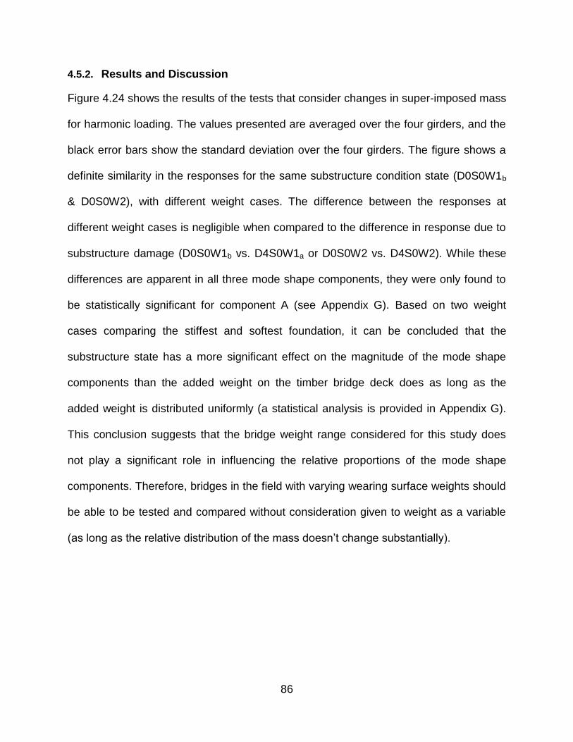
86


Figure 4.24 shows the results of the tests that consider changes in super-imposed mass

for harmonic loading. The values presented are averaged over the four girders, and the

black error bars show the standard deviation over the four girders. The figure shows a

definite similarity in the responses for the same substructure condition state (D0S0W1b

& D0S0W2), with different weight cases. The difference between the responses at

different weight cases is negligible when compared to the difference in response due to

substructure damage (D0S0W1b vs. D4S0W1a or D0S0W2 vs. D4S0W2). While these

differences are apparent in all three mode shape components, they were only found to

be statistically significant for component A (see Appendix G). Based on two weight

cases comparing the stiffest and softest foundation, it can be concluded that the

substructure state has a more significant effect on the magnitude of the mode shape

components than the added weight on the timber bridge deck does as long as the

added weight is distributed uniformly (a statistical analysis is provided in Appendix G).

This conclusion suggests that the bridge weight range considered for this study does

not play a significant role in influencing the relative proportions of the mode shape

components. Therefore, bridges in the field with varying wearing surface weights should

be able to be tested and compared without consideration given to weight as a variable

(as long as the relative distribution of the mass doesn‟t change substantially).

87

Figure 4.24. Mode shape components from harmonic excitation for different weight

cases

Table 4.4 shows the effect of the bridge weight on the first natural frequency. A softer

foundation and a heavier structure both reduce the natural frequency. It is unclear from

the data which has a greater effect; however, it is important to note that both are key

variables determining the natural frequency. This suggests that natural frequency alone

cannot be used as an indication of superstructure stiffness, as the substructure and

bridge weight both play large roles. Weight and substructure stiffness must both be

considered if the natural frequency is to be used as an indication of superstructure

stiffness.

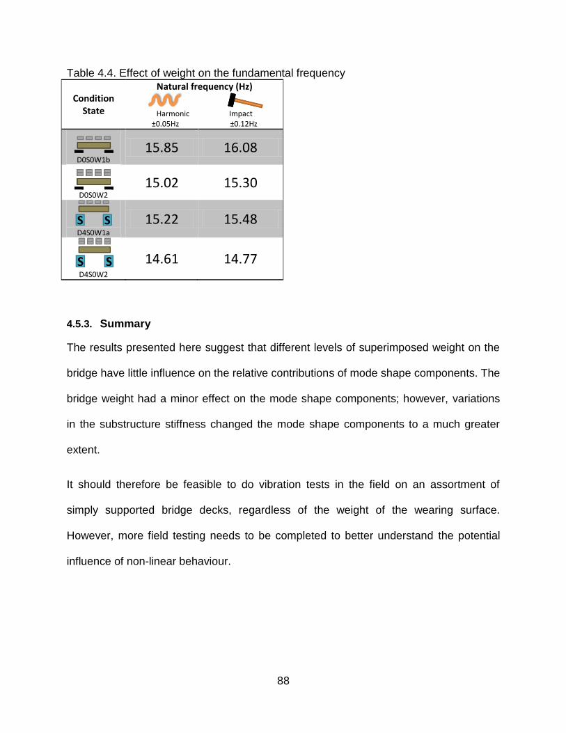
88

Table 4.4. Effect of weight on the fundamental frequency

Condition State


Harmonic Impact

±0.05Hz ±0.12Hz

D0S0W1b

15.85 16.08

D0S0W2

15.02 15.30

D4S0W1a

15.22 15.48

D4S0W2

14.61 14.77

4.5.3. Summary

The results presented here suggest that different levels of superimposed weight on the

bridge have little influence on the relative contributions of mode shape components. The

bridge weight had a minor effect on the mode shape components; however, variations

in the substructure stiffness changed the mode shape components to a much greater

extent.

It should therefore be feasible to do vibration tests in the field on an assortment of

simply supported bridge decks, regardless of the weight of the wearing surface.

However, more field testing needs to be completed to better understand the potential

influence of non-linear behaviour.

89

4.6. SUPERSTRUCTURE DAMAGE DETECTION

4.6.1. Overview

The VBDD methods presented in this study thus far have inferred damage considering

a single vibration test, while comparing results from a range of substructure condition

states. In this section, the application of more conventional VBDD methods is described;

these rely on the direct comparison the mode shape of the bridge in a given state to that

in a previous condition state. The methods employed were the change in mode shape

(Equation 2.1) and the change in curvature methods (Equation 2.3), as these are

among the most widely used approaches in the literature and relatively easy to

implement. Damage considered in this phase of the study consisted of small-scale

damage to the superstructure.

This section also describes the application of the change in mode shape and change in

curvature methods to a bridge with both substructure damage and small-scale

superstructure damage. The intent of this final analysis was to try to better understand

the effect substructure damage has on detecting superstructure damage and vice versa.

4.6.2. Superstructure Damage Detection

The results for the superstructure damage detection tests are presented in this section,

considering only the rigid-rigid (D0) support case. To apply VBDD methods to the

superstructure, the substructure components, B and C, were removed and the flexural

deformations (A) were re-normalized using girder-normalization enclose a unit-area.

Figure 4.25 and Figure 4.26 show the distribution of change in mode shape and change

in curvature, respectively, for the condition state consisting of a cut at the centre of

90

Girder 2 (S1). It is apparent that the largest changes occurred in both parameters in

Girder 2, suggesting that damage has been detected on Girder 2 (level 1 detection).

However, the location along the girder was not successfully identified (level 2 detection),

since the largest peaks in the damage parameter plots do not coincide with the known

damage location. Although the data are not presented here, it was found that the

damage could not be detected using impact excitation; mode shapes produced using an

impact were found to exhibit substantially more variability (Section 4.2.4) and the effect

of the damage was not great enough to make detection possible.

Figure 4.25. Change in mode shape -

D0S0W1c vs. D0S1W1 (harmonic)

Figure 4.26. Change in curvature – D0S0W1c vs. D0S1W1 (harmonic)

Figure 4.27 and Figure 4.28 show the results of tests with damage to Girder 4 (S2)

using Damage Case S1 as the base case. In both figures, it is clear that damage is

most likely to have occurred on Girder 4, and the large positive peaks on the figures

indicate that the damage was likely located approximately 2000 mm from the left

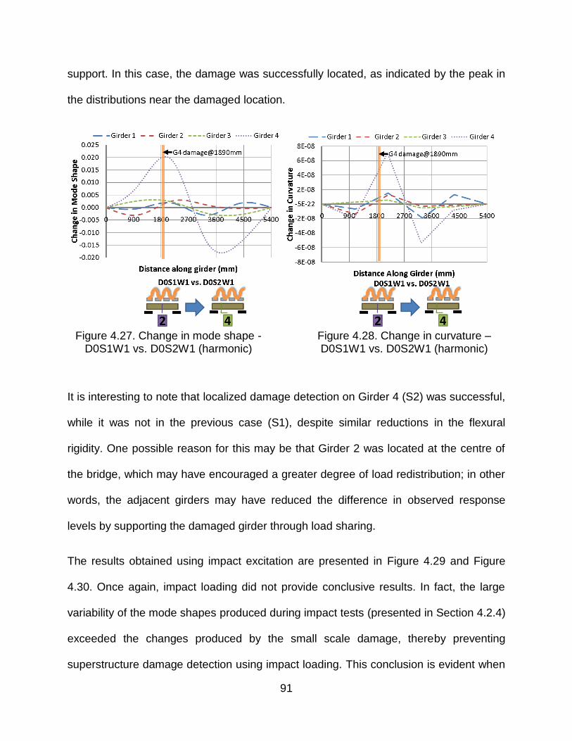
91

support. In this case, the damage was successfully located, as indicated by the peak in

the distributions near the damaged location.


D0S1W1 vs. D0S2W1 (harmonic)

Figure 4.28. Change in curvature – D0S1W1 vs. D0S2W1 (harmonic)

It is interesting to note that localized damage detection on Girder 4 (S2) was successful,

while it was not in the previous case (S1), despite similar reductions in the flexural

rigidity. One possible reason for this may be that Girder 2 was located at the centre of

the bridge, which may have encouraged a greater degree of load redistribution; in other

words, the adjacent girders may have reduced the difference in observed response

levels by supporting the damaged girder through load sharing.

The results obtained using impact excitation are presented in Figure 4.29 and Figure

4.30. Once again, impact loading did not provide conclusive results. In fact, the large

variability of the mode shapes produced during impact tests (presented in Section 4.2.4)

exceeded the changes produced by the small scale damage, thereby preventing

superstructure damage detection using impact loading. This conclusion is evident when

92

comparing the multiple large peaks in Figures 4.29 and 4.30 compared to the single

large peak featured in Figures 4.27 and 4.28.


D0S1W1 vs. D0S2W1 (impact)

Figure 4.30. Change in curvature – D0S1W1 vs. D0S2W1 (impact)

4.6.3. Substructure and Superstructure Interactions

The final area to be investigated in this part of the study was the interaction of

superstructure damage with substructure damage. To apply superstructure damage

detection in this study, the substructure movement (B and C) was first removed from the

mode shape; the flexural response, A, was then unit-area normalized again.

Consequently, this section compares the flexural deformations independent of

substructure movement.

In Figure 4.31 and Figure 4.32, the change in mode shape and change in mode shape

curvature are plotted, comparing two condition states for which there was a change in

substructure condition, as well as in the superstructure condition. The substructure

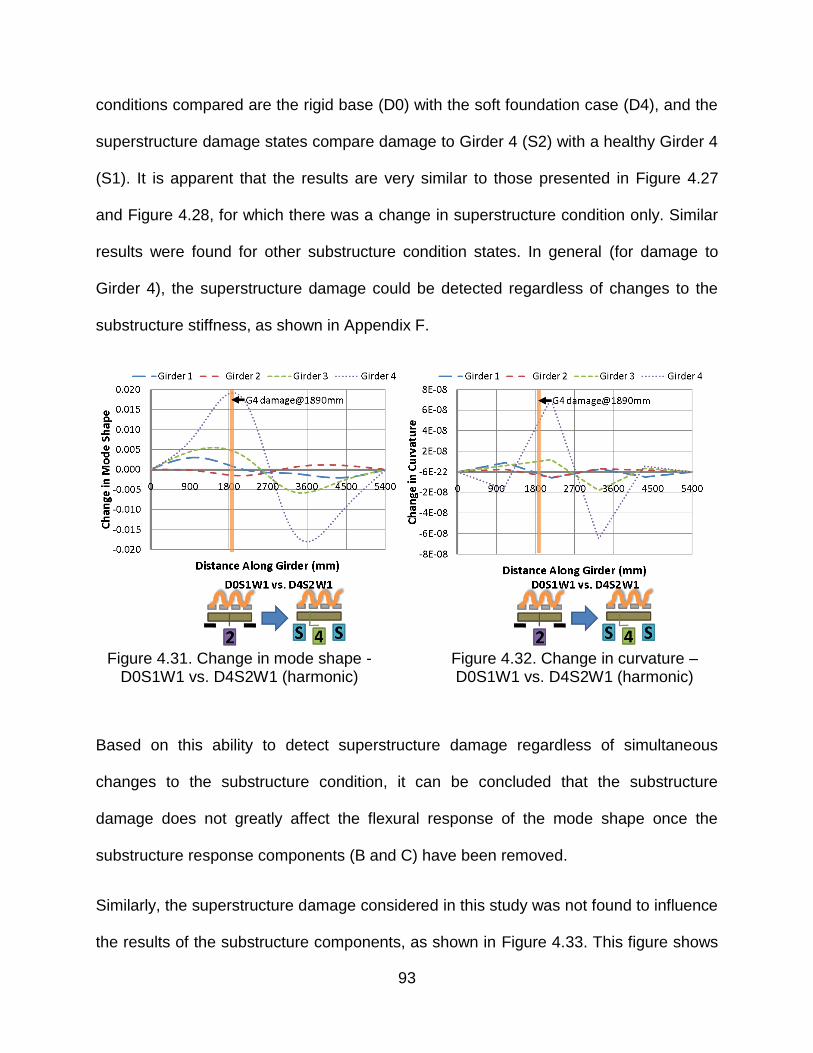
93

conditions compared are the rigid base (D0) with the soft foundation case (D4), and the

superstructure damage states compare damage to Girder 4 (S2) with a healthy Girder 4

(S1). It is apparent that the results are very similar to those presented in Figure 4.27

and Figure 4.28, for which there was a change in superstructure condition only. Similar

results were found for other substructure condition states. In general (for damage to

Girder 4), the superstructure damage could be detected regardless of changes to the

substructure stiffness, as shown in Appendix F.


D0S1W1 vs. D4S2W1 (harmonic)

Figure 4.32. Change in curvature – D0S1W1 vs. D4S2W1 (harmonic)

Based on this ability to detect superstructure damage regardless of simultaneous

changes to the substructure condition, it can be concluded that the substructure

damage does not greatly affect the flexural response of the mode shape once the

substructure response components (B and C) have been removed.

Similarly, the superstructure damage considered in this study was not found to influence

the results of the substructure components, as shown in Figure 4.33. This figure shows

94

the mode shape components for three cases of superstructure condition, while the

substructure condition remained constant at the “soft-hard” (D5) condition state. Given

the same foundation stiffness, there was little change observed in the mode shape

components when the superstructure condition states changed. A statistical analysis

using a Student‟s t-test, provided in Appendix G, further supports this observation

considering all remaining substructure cases. It is important to note that the foundation

supports were switched out between tests, meaning that the bearing conditions were

not exactly the same for the three tests illustrated in Figure 4.33 due to unintended

variations in nominally similar test setups.

The observations made from Figure 4.33 may not be the case for larger forms of

superstructure deterioration, which should be studied further. Specifically, it is

suspected that the foundation will appear relatively stiffer (in the form of minimal

substructure movement) when a highly flexible superstructure is present and the mode

shape is broken down into components. In other words, only relative movements can be

extracted when a normalized mode shape is deconstructed into the three mode shape

components. Also, it is possible that larger forms of shear damage, as reported by

Peterson (2001), may also produce similar mode shape components to those

associated with foundation deterioration.

95

Figure 4.33. Mode shape components for the bridge with a constant foundation case

D6, but under various superstructure condition states

As previously shown (Wang et al. 2009), the areas under the change in mode shape

(Equation 2.5) and change in curvature (Equation 2.6) plots can be a good indication of

Level 1 damage detection (identifying the presence of damage). Figure 4.34 compares

the area under the change in mode shape (and change in curvature) for each girder

given a specific base case. It should be noted that the plot corresponds to changes in

the renormalized superstructure movement, where the substructure movement was

removed. Figure 4.34 uses the rigid bridge state as the base case, and compares the

area under the change in flexural mode shape to other bridge condition states. Two

superstructure condition states are compared (S1 and S2), as well as four substructure

condition states (D0, D4, D5, and D6).

A threshold value is defined on Figure 4.34 and Figure 4.35 with a dashed line for the

area under the change in mode shape and change in curvature vectors. Values that

exceed the threshold indicate that there was a statistically significant change in the

96

response of the girder as compared to the base case, which suggests that damage has

occurred (α=0.0013). The threshold was established to be three standard deviations

away from the mean change in area vector when considering an undamaged

superstructure state with varying substructure stiffness. More details on the mean,

standard deviation and methodology used to establish a threshold are available in

Appendix F.

Figure 4.34 shows that damage has been detected on Girder 4 when it was present.

Changes in substructure flexibility had little effect on the area under the change in mode

shape vector.

Conversely, when the damage to Girder 2 was used in this analysis, the results were

once again not as conclusive, as shown in Figure 4.35. The VBDD method was not

successful at level 1 damage detection for superstructure damage. Once again, this is

likely due to the load redistribution that occurred with the damage to Girder 2.

97

Figure 4.34. Area under the change in mode shape and change in curvature plots when comparing the base case (D0S1W1) to other superstructure and substructure damage

states

98

Figure 4.35. Area under the change in mode shape and change in curvature plots when comparing the base case (D0S0W1) to other superstructure and substructure damage

states

99

4.6.4. Summary

Small-scale damage to the superstructure was successfully localized using harmonic

excitation, but only when the damage occurred on an external girder. It is likely that the

damage would have to be more severe for damage detection to be successful using

impact excitation; however, larger damage cases would have to be considered to

confirm this.

The results also showed that the superstructure response could be distinguished from

the substructure response. The substructure condition did not significantly affect the

ability to detect damage to the superstructure. Furthermore, preliminary studies using

small-scale superstructure damage indicated that the substructure response was not

significantly affected by superstructure damage. However, this may not be the case

when significant changes in the superstructure bending stiffness are considered.

4.7. PRACTICAL APPLICATION

4.7.1. Overview

The method of deconstructing a mode shape into superstructure and substructure

components appears to have great potential to identify the condition of the substructure

of the bridge using a single vibration test. However, in the laboratory, the approach was

demonstrated comparing the vibration signatures associated with known condition

states. As such, further research is required to gather vibration signatures from a wide

range of timber bridges in the field. This section presents some recommendations for

practical testing in the field.

100

In practice, dynamic bridge tests are easier to carry out when impact loading is used for

excitation. Additionally, the number of sensors available may be fewer than what was

considered for this study. To test the influences of these two factors, the mode shape

component method was evaluated using only impact loading and a smaller number of

sensors on the timber bridge deck.


The timber bridge in the laboratory was intensively instrumented, with the vertical

movement of the bridge measured at 22 points. This extent of instrumentation would be

very time consuming to implement in the field. Figure 4.36 shows a more limited

accelerometer configuration that could be more easily implemented in the field. This

configuration includes an accelerometer near the centre of the girder and over both

supports for all the girders on the bridge.

Although the hydraulic shaker remained attached at the centre of the bridge for all

testing, the excitation for all results presented in this section were obtained using impact

loading applied near the centre of the bridge (as described in Section 3.3.2). Impact

loading is easy to implement in the field and has already been shown to provide

adequate information to apply VBDD methods (Section 4.3.5). Figure 4.37 shows the

bridge-normalized first flexural mode shape for the non-uniform foundation case (D3)

generated using impact loading and the limited accelerometer configuration.

101

Figure 4.36. Plan view of the bridge, showing accelerometer locations for practical

application (dimensions in mm)

Figure 4.37. First flexural mode shape produced using limited sensors

By using a cubic spline interpolation function (Luong 2009) over each individual girder,

the mode shape was interpolated between sensor locations to create a smooth

response with zero curvature at supports. The girder mode shapes were then girder-

normalized to have a unit-area under each girder. The mode shape components were

102

then extracted, with the results shown in Figure 4.38. By comparing Figure 4.38 to the

more intensively instrumented equivalent shown in Figure 4.22, it is apparent that

interpretation of the results was not adversely affected to any significant extent by

reducing the number of sensors by nearly half. In both cases (intensive and sparse

instrumentation), it is clear that the differential support movement (component B)

increased in a relative sense with softening supports and the flexural deformations

(component A) decreased with flexible substructure conditions. These conclusions are

shown further in Table 4.5 and in a statistical analysis provided in Appendix G.

Figure 4.38. Mode shape components for substructure condition states using the limited

accelerometer configuration

Table 4.5 presents the change in mode shape components from the base case

(D0S0W1a) for three condition states, considering both intensive and sparse

instrumentation configurations. The change in the relative contribution of the differential

103

support movement (∆B) was not affected by the instrumentation levels, suggesting that

intensive instrumentation may not be required. The sparse instrumentation configuration

resulted in a change in differential substructure response that was, on average, 1.74%

higher than the values produced using intensive instrumentation.

As shown in previous results for detection of substructure damage, flexural

deformations (A) are important only in the sense that they provide a basis for evaluating

how significant the substructure components are. Although the flexural deformations (A)

cannot be totally discounted in identifying damage to the substructure, it seems that a

single measurement is enough to quantify the flexural component (A).

Table 4.5. Change in mode shape components relative to the base foundation case (D0S0W1a), for impact loading considering 22 sensors vs. 12 sensors 22 Sensors

Impact

D0S0W1a


∆A ∆B ∆C

12 Sensors Impact

D0S0W1a


∆A ∆B ∆C

D0S0W1b

0.000 -0.016 0.011

D0S0W1b

0.001 -0.017 0.011

D1S0W1

-0.017 0.032* -0.015

D1S0W1

-0.017 0.032* -0.016

D2S0W1

-0.068* 0.094* -0.025

D2S0W1

-0.069* 0.096* -0.027

*Change is statistically significant (α=0.1)

104

4.7.3. Summary

Limiting the number of sensors had little effect on the ability of the mode shape

deconstruction method to infer substructure damage, provided that sensors were placed

over the supports to obtain a good measurement of substructure movement.

Furthermore, at least one sensor was required on each girder between the supports to

quantify the flexural component. In other words, each girder must be instrumented by

three sensors to adequately quantify damage using the deconstructed mode shape, one

measuring each component.

105

5. PATTERN RECOGNITION USING NEURAL NETWORKS

5.1. OVERVIEW

This chapter summarizes the limited work that was done using neural networks to aid in

pattern recognition using the response signatures gathered during this research

program. It is important to note that this chapter is not an extensive investigation of

neural networks; rather, the intent was only to provide a brief analysis of the data

recovered from this study. This analysis is included to serve as an example of how

pattern recognition can be used on deconstructed mode shapes to identify substructure

stiffness and infer possible damage.

5.2. BACKGROUND

Artificial neural networks were created to imitate, with a computer, a human‟s decision-

making and learning capabilities. Computers are very good at following rules and doing

repetitive calculations, yet their ability to learn and make their own rules is very limited if

the logic is not already programmed. Neural networks provide the potential to allow

computers to learn and solve complex problems where the pattern cannot easily be

described by pre-programmed routines. This is done by modelling a portion of the

massive and complex system of neurons that is seen in the human brain to do a very

specific task. The end result is an artificial neural network with a broad spectrum of

106

applications consisting of a highly parallel system that is densely connected, similar to

that of the human brain (Dayhoff 1990).

Pattern recognition is just one of the applications that neural networks do extremely

well. For pattern recognition, the network is trained with a given set of inputs and the

corresponding known outputs so that the network can later recognize patterns without

being given the output.

Figure 5.1 illustrates a simple single layer network. In this particular network, the inputs

are multiplied by weighting factors, and the results are subsequently added together at

the node. The resulting sum is then compared to a threshold value, and a 0 or 1 is

returned as an output depending on whether the threshold is exceeded. The weighting

factors and thresholds are determined through the training process based on the

training data. More complex neural networks would include more layers and nodes.

Figure 5.1. A simple artificial neural network (Gurney 1997)

107

Farrar and Doebling (1999) state that pattern recognition techniques need to be

implemented to advance vibration-based damage detection techniques. These

techniques could potentially be similar to those that have been practically applied to the

monitoring of rotating machinery by the use of databases and statistical pattern

recognition. In the current research, neural networks were used as a tool for pattern

recognition so that specific bridge deficiencies could be classified using a database of

known bridge states. Specifically, the data gathered in this study were used for

classifying the condition state of the substructure on the test bridge.

5.3. EXPERIMENTAL PROGRAM

Development and implementation of a neural network is a difficult process that is

outside the scope of this research. As an alternative, all neural network analyses for this

research program were performed using free software called A.I. Solver Studio (2007)

by Perseptio. The A.I. Solver Studio user manual by Perseptio (2007) states,

“A.I. Solver Studio is a unique pattern recognition application that deals with

finding optimal solutions to classification problems and uses several powerful and

proven artificial intelligence techniques including neural networks, genetic

programming and genetic algorithms. No special knowledge is required of users

as A.I. Solver Studio manages all the complexities of the problem solving

internally.”

As suggested, the application excels at classification problems using neural networks

for pattern recognition. The program is very simple to use; however, the user has very

108

little opportunity to understand the architecture and complexity of the developed artificial

neural network.

The intent of this chapter was to employ a neural network for its pattern recognition

abilities to classify the foundation stiffness based on the mode shape component inputs

provided (substructure and superstructure movement). In Table 5.1, the mode shape

component inputs produced using impact loading are listed in the six columns on the

right; these include the average value and standard deviation of the substructure

movement (B and C), as well as those of the superstructure movement (A) over the four

bridge girders. For a specific bridge state, the average amplitude of a mode shape

component was calculated based on the average of that component from the four

girders for the test. Similarly, the standard deviation was calculated based on the

amplitudes from the four girders. The desired output was the foundation stiffness, which

was classified as “hard” for all setups with rigid or oak supports, or “soft”, for any

configuration that included a pine support (signifying a damaged support).

The data in Table 5.1 was used to train the neural network in A.I. Solver Studio. The

software had the option to select from multiple complexity levels (trivial to unsolvable)

and also allowed for genetic programming within the neural network to aid in the training

process. The analysis in this study consisted of a neural network of „trivial‟ complexity.

The genetic programming, “hindsight” and “over-fitting prevention” capabilities available

in the software were all disabled. These features were not included because they were

either not applicable, or the data set was not large enough to warrant their use.

109

As suggested in the software user‟s manual, 20% of the data was withheld from training

to be solely used for testing the neural network (Perseptio 2007). Bridge configurations

corresponding to the last superstructure condition state (S2) were selected for the

verification exercise because this condition state included all four foundation

configurations that had previously been used in the training process (see a description

of the condition states in Section 3.8.4). The portion of the data used for network

verification is shown in Table 5.2.

Table 5.1. Mode shape component data used to train the model

Bridge Configuration

Fdn Stiffness

Average A

Average B

Average C

Std Dev. A

Std Dev. B

Std Dev. C

D0S0W1a Hard 0.74135 0.04655 0.21210 0.030615 0.01537 0.044001

D1S0W1 Hard 0.72447 0.07809 0.19744 0.043199 0.0114 0.03483

D2S0W1 Soft 0.67296 0.14033 0.18672 0.049607 0.010711 0.040126

D3S0W1 Soft 0.70700 0.07949 0.21351 0.019999 0.073658 0.054731

D0S0W1b Hard 0.74531 0.03078 0.22391 0.017606 0.045442 0.05713

D0S0W2 Hard 0.74342 0.03941 0.21717 0.009538 0.051387 0.058949

D4S0W1a Soft 0.66522 0.08011 0.25467 0.026734 0.008399 0.019461

D4S0W2 Soft 0.68493 0.07373 0.24133 0.03003 0.021916 0.012236

D0S0W1c Hard 0.75414 0.03952 0.20634 0.008655 0.02354 0.030822

D4S0W1b Soft 0.68679 0.05445 0.25877 0.022491 0.008178 0.030135

D5S0W1 Hard 0.71892 0.05362 0.22746 0.010321 0.01367 0.022385

D6S0W1 Soft 0.69120 0.09895 0.20985 0.020302 0.010073 0.029695

D0S1W1 Hard 0.75823 0.03834 0.20344 0.007341 0.023474 0.028791

D4S1W1 Soft 0.68810 0.04737 0.26453 0.016931 0.005341 0.016583

D5S1W1 Hard 0.72218 0.05648 0.22133 0.009944 0.005653 0.013253

D6S1W1 Soft 0.69468 0.09360 0.21172 0.027986 0.039248 0.012413

Table 5.2. Mode shape component data used to test the model

Bridge Configuration

Fdn Stiffness

Average A

Average B

Average C

Std Dev. A

Std Dev. B

Std Dev. C

D0S2W1 Hard 0.76644 0.04069 0.19286 0.012902 0.01751 0.028322

D4S2W1 Soft 0.68769 0.06069 0.25162 0.027508 0.019835 0.011224

D5S2W1 Hard 0.71294 0.06375 0.22331 0.008128 0.021498 0.025555

D6S2W1 Soft 0.70003 0.08776 0.21221 0.033032 0.017355 0.016601

110

5.4. RESULTS

The training process was short, requiring only three iterations for convergence to the

final network. This suggested that the resulting neural network was relatively simple. All

the training data from the four foundation condition states considered (two hard and two

soft) converged to the correct solution, as shown in the screenshot (Figure 5.2).

Additionally, it is apparent that the neural network predicted the foundation stiffness of

the testing data with 100% reliability. This suggests that there was enough difference in

the data sets to successfully classify the foundation stiffness as either hard or soft.

Figure 5.2. A.I. Solver user interface displaying results from both training and testing of

the neural network

Figure 5.3 presents a small portion of the data used in the training and testing

processes (two of the six columns from Table 5.1 and 5.2 in graphical form). In this

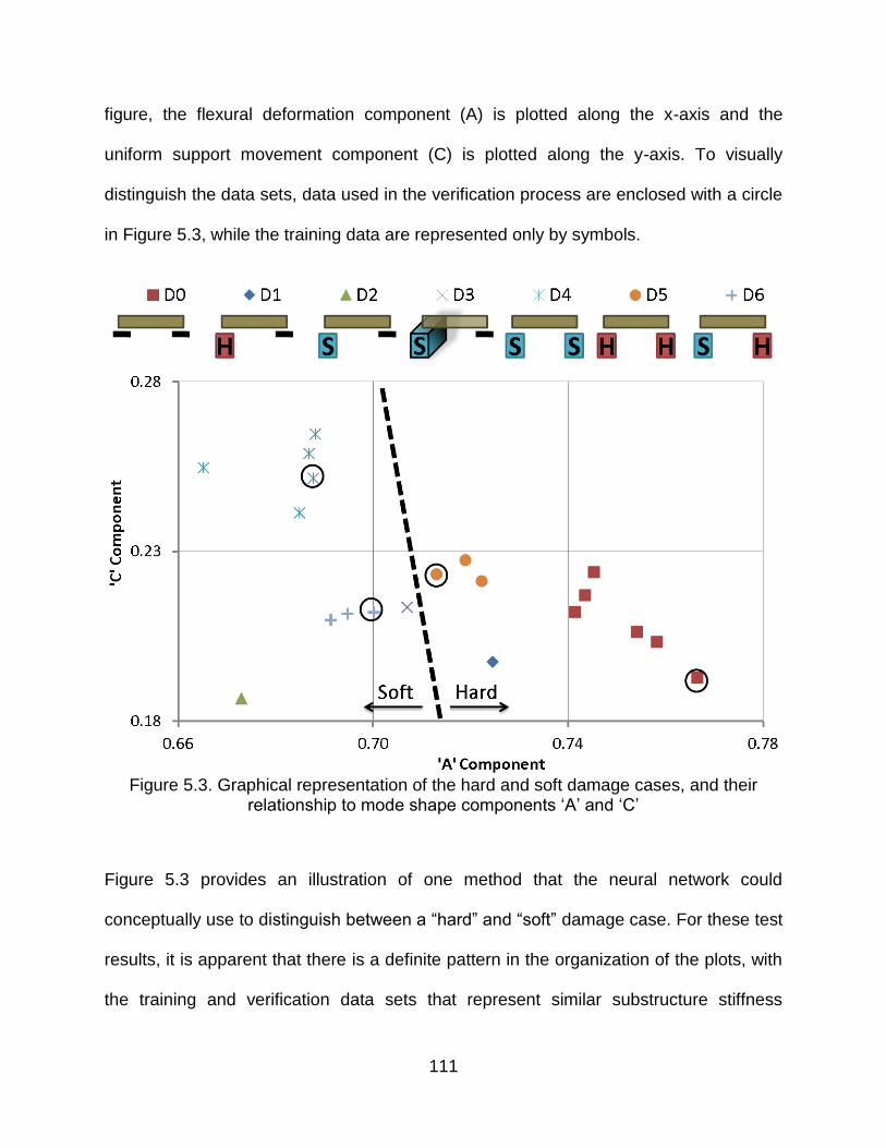
111

figure, the flexural deformation component (A) is plotted along the x-axis and the

uniform support movement component (C) is plotted along the y-axis. To visually

distinguish the data sets, data used in the verification process are enclosed with a circle

in Figure 5.3, while the training data are represented only by symbols.

Figure 5.3. Graphical representation of the hard and soft damage cases, and their

relationship to mode shape components „A‟ and „C‟

Figure 5.3 provides an illustration of one method that the neural network could

conceptually use to distinguish between a “hard” and “soft” damage case. For these test

results, it is apparent that there is a definite pattern in the organization of the plots, with

the training and verification data sets that represent similar substructure stiffness

112

conditions being closely grouped together and well separated from other data

groupings. The fact that there is no overlap observed between condition state data

could account for the result that unique, non-ambiguous classifications were possible

using this approach. It should be noted that the non-uniform substructure stiffness state

(D3) is located very close to the dashed line plotted in Figure 5.3 that defines an

approximate boundary separating “hard” and “soft” condition results. As a result, to

recognize this bridge state as being “soft” would also require consideration of the

standard deviation values shown in Table 5.1. Specifically, the large standard deviation

of the differential support movement for the non-uniform support case could indicate a

“soft” support, as demonstrated by Figure 4.22 and the F-test on variance in Appendix

G.

5.5. CONCLUSION

This chapter summarized the results of a limited study that applied pattern recognition

software to classify substructure condition states. Although the study gave promising

results, in that all substructure stiffness conditions were accurately classified, it was only

intended to provide an indication of the potential of this approach as a starting point for

future research. To extend this study to field applications, it is suggested that a wide

range of timber bridges be tested dynamically in conjunction with an assessment

conducted by an experienced bridge inspector to create an extensive database of

response signatures that can be correlated to the bridge state identified by the

inspector. Through creating the database of bridges with known condition states, further

research can be undertaken to determine the practical use of pattern recognition

techniques to classify the bridge state given the response signatures.

113

6. CONCLUSIONS AND RECOMMENDATIONS

6.1. SUMMARY

Vibration-based damage detection (VBDD) has the potential to serve as an integral part

of a routine structural health monitoring program. The study described in this thesis

considered the application of VBDD methods as a potential solution to the challenge of

properly assessing the large and deteriorating inventory of timber bridge infrastructure

in Saskatchewan. VBDD methods offer a quick and economical inspection method that

can simultaneously evaluate the entire structure for damage. Typically, deterioration in

timber bridges occurs within the substructure at locations not readily accessible to

current inspection methods. The focus of this study was to apply VBDD methods to

assess substructure stiffness on a simply supported timber bridge in the laboratory.

The variables that were considered were the excitation method, the amount of

superimposed mass on the deck, damage to the superstructure and realistic stiffness

changes to the substructure. It was found that damage to the superstructure could be

assessed based on observed changes in response patterns relative to a baseline case,

whereas changes in substructure stiffness could be detected considering the dynamic

response using a single vibration test.

114

6.2. CONCLUSIONS

This research included an experimental program designed to assess the influence of

substructure deterioration on the dynamic properties of a simply supported timber

bridge. Dynamic testing was carried out on a 5.9 m long by 2.44 m wide segment of a

timber deck assembly removed from a decommissioned bridge. The significant

observations and conclusions from this study are listed below.

Decreasing the substructure stiffness of the timber bridge resulted in additional

movement over the supports and a reduction in the natural frequency of the

bridge assembly.

Substructure deterioration could be inferred by a simple deconstruction of the

first fundamental mode shape without reference to baseline (prior to damage

condition) measurements.

o The first flexural mode could be adequately described using three primary

components: flexural deformations resembling the fundamental mode

shape of a simply supported beam (component A), rigid body rotation

associated with differential support movement (component B), and rigid

body motion due to uniform support movement at both ends of the girder

(component C). The relative contributions of these three components

compared to the response of other substructure bridge states provided

valuable information regarding the presence and possible location of

support deterioration. More specifically, substructure damage influenced

these components as follows:

115

i. Flexural response: The flexural component (A) was more

prominent when the substructure was stiffer, resulting in a relative

reduction in contribution of the substructure components.

ii. Differential support movement: This component increased as the

difference between the support stiffness at the two ends of the

girder increased.

iii. Uniform support movement: This component represented the

relative contribution of uniform substructure movement to the

fundamental mode shape of the bridge. Uniform support

movement was always present (even in stiffest substructure

cases) and was likely caused by the compressibility of the timber

pile cap and bearing region of the girder. However, an increase in

the flexibility of the foundation below the cap also caused a further

increase in this component.

Neither the amount of uniformly distributed superimposed mass placed on the

deck nor imposed superstructure damage affected the relative amplitudes of the

mode shape components. Therefore, for the range of these variables considered,

it can be concluded that superimposed mass and superstructure damage did not

influence the effectiveness of substructure damage detection for the method

proposed.

Small-scale superstructure damage was detected using VBDD methods that

relied on a comparison to a baseline response using harmonic loading. In this

case, the imposed damage caused a 38% reduction in the flexural rigidity of an

116

outer girder on a bridge consisting of four girders. Damage to the outer girder at

1890 mm from one support was identified and successfully localized. Small-scale

damage could not be located for damage to an internal girder (possibly due to

the greater degree of load sharing available to the interior girders) or by using

impact excitation.

Simultaneous damage to the superstructure and substructure could be

differentiated and successfully detected independently.

Steps were taken to better understand testing protocols for future research in the

field. The main observations in this regard are listed below:

o Mode shapes gathered from impact loading were adequate for detecting

substructure damage, but were not adequate for detecting the small

degree of damage to the superstructure that was considered in this

research.

o To apply the substructure damage detection methods described in this

research, instrumentation is required at each support, while a single

measurement at the mid-span of each girder is sufficient for the relative

superstructure response. The superstructure need only be heavily

instrumented for the superstructure damage detection methods requiring a

baseline response.

Pattern recognition using neural networks and a database of known bridge

condition states may be a feasible method to classify a timber bridge‟s

substructure condition in the field. However, a great deal of field research still

needs to be done before this methodology can be implemented in practice.

117

6.3. RECOMMENDATIONS AND FUTURE RESEARCH

It should be noted that the scope of the present study was limited to the bridge, support

condition states and environmental conditions investigated as part of this laboratory

investigation. It is recognized that the practical application of this approach in the field

will introduce a wide range of additional complexities, including an infinite variety of

potential structural health states for both the superstructure and substructure, as well as

variable and changing ambient conditions. As such, in order to apply this approach in

practice, it is recommended that further research be conducted to investigate the in-situ

dynamic response characteristics of actual timber bridges of various sizes and

configurations with varying degrees of substructure and superstructure deterioration.

Also, additional field research is likely required to better understand the non-linear

behaviour of timber bridges given a wide range of bridges with different weights.

It is recommended that the preliminary pattern recognition methods used in this study to

characterize the structural condition of timber bridges be applied in the field and

investigated further. There is considerable work that is still required to calibrate and

validate the method. Primarily, a database of actual bridges must be assembled,

covering a wide range of substructure stiffness values, superstructure stiffness values,

bridge deck weights and geometries, soil types, moisture conditions, and ambient

environmental (temperature, humidity, etc.) conditions.

118

REFERENCES

Beauregard, C. J., Sparling, B. F., and Wegner, L. D. 2010. Vibration-based damage

detection for support softening under a simply supported timber bridge. 2nd

International Structures Specialty Conference, CSCE, Winnipeg, Manitoba,

Canada, Paper No. ST-071.

Brashaw, B. K., Vatalaro, R., Wang, X., Sarvela, K., and Wacker, J. 2008. Development

of flexural vibration inspection techniques to rapidly assess the structural health of

rural bridge systems. Report No. CTS 08-22, Intelligent Transportation Systems

Institute Center for Transportation Studies, Minneapolis, Minnesota.

Burkett, J. L. 2005. Benchmark studies for structural health monitoring using analytical

and experimental models. M.Sc. Thesis, Department of Civil and Environmental

Engineering, University of Central Florida, Orlando, USA.

Butterworth, S. 1930. On the theory of filter amplifiers. Experimental Wireless and the

Wireless Engineer, 7: 536-541.

Dayhoff, J. E. 1990. Neural network architectures: an introduction. Van Nostrand

Reinhold, New York, N.Y.

Doebling, S. W., Farrar, C. R., and Prime, M. B. 1998. A summary review of vibration-

based damage identification methods. Shock and Vibration Digest, 30(2): 91-105.

119

Donovan, K. A. 2004. Field tests of timber railroad bridge piles. M.Sc. Thesis, Civil

Engineering, Texas A&M University, Texas, USA.

Emerson, R. N., Pollock, D. G., Kainz, J. A., Fridley, K. J., McLean, D. L., and Ross, R.

R. 1998. Nondestructive evaluation techniques for timber bridges. 5th World

Conference on Timber Engineering, Presses PolyTechniques et Universitaires

Romandes, Montreux, Switzerland, pp. 670-677.

Farrar, C. R., and Doebling, S. W. 1999. Damage detection II: field applications to large

structures. Modal analysis and testing, Nato science series, J. M. Silva and N. M.

Maia, eds., Kluwer Academic Publishers, Dordrecht, Netherlands, 345-378.

Fayyadh, M. M., and Razak, H. A. 2012. Condition assessment of elastic bearing

supports using vibration data. Construction and Building Materials, 30: 616-628.

Fleming, K., Weltman, A., Randolph, M., and Elson, K. (2009). Pile engineering 3rd

edition. Taylor & Francis, New York, NY:

Foti, S., and Sabia, D. 2011. Influence of foundation scour on the dynamic response of

an existing bridge. Journal of Bridge Engineering, 16(295): 295-304.

Gurney, K. 1997. An Introduction to neural networks. UCL Press, London, England,

U.K.

Li, J., Samali, B., and Crews, K. I. 2004. Determining individual member stiffness of

bridge structures using a simple dynamic procedure. Acoustics Australia, 32(1): 9-

12.

120

Luong, B. 2009. Spline derivative - spline1d.m [MATLAB function]. Available from

MATLAB Central: http://www.mathworks.com/matlabcentral/fileexchange/24996-

spline-derivative [cited 21 October 2011].

Martenson, A. 2003. Short- and long-term deformations of timber structures. Timber

engineering, S. Thelandersson and H. J. Larsen, eds., John Wiley & Sons Ltd,

West Sussex, England, 221-240.

Muchmore, F. W. 1986. Designing timber bridges for long life. Transportation

Reasearch Record, 1053: 12-17.

National Instruments. 2005. Labview - TM v.8.0 [computer software]. Austin, Texas.

Ou, F. L., and Weller, C. 1986. An overview of timber bridges. Transportation Research

Record, 1053: 1-12.

Pandey, A. K., and Biswas, M. 1994. Damage detection in structures using changes in

flexibility. Journal of Sound and Vibration, 169(1): 3-17.

Pandey, A. K., Biswas, M., and Samman, M. M. 1991. Damage detection from changes

in curvature mode shapes. Journal of Sound and Vibration, 145(2): 321-332.

Perseptio. 2007. A.I Solver Studio - Version 1.0 [software]. Available from Perseptio:

http://www.perseptio.com/Products.aspx [cited 13 October 2011].

Perseptio. 2007. A.I. Solver Studio - user manual. Available from Perseptio:

http://www.perseptio.com/AISolverStudioManual.aspx [cited 13 October 2011].

121

Peterson, S. T., McLean, D. I., and Pollock, D. G. 2003. Application of dynamic system

identification to timber bridges. Journal of Structural Engineering, 129(1): 116-124.

Peterson, S. T., McLean, D. I., Symans, M. D., Pollock, D. G., Cofer, W. F., Emerson,

R. N., et al. 2001. Application of dynamic system identification to timber beams II.

Journal of Structural Engineering, 127(4): 426-432.

Pham, T. 2009. The influence of thermal effects on structural health monitoring of

attridge drive overpass. M.Sc. Thesis, Department of Civil Engineering, University

of Saskatchewan, Saskatoon, Canada.

Poulos, H. G., and Davis, E. H. 1980. Pile foundation analysis and design. Wiley, New

York, N.Y.

Ramirez, R. W. 1985. The FFT: fundamentals and concepts. Prentice-Hall, Englewood

Cliffs, New Jersey, USA.

Ritter, M. A. 1990. Timber bridges: design, construction, inspection and maintenance.

Report No. EM 7700-8, United States Department of Agriculture Forest Service.

Washington, DC.

RTA. 2008. Timber bridge manual. Roads and Traffic Authority of NSW, New South

Wales, Australia.

Rytter, A. 1993. Vibration-based inspection of civil engineering structures. Ph.D.

Dissertation, Department of Building Technology and Structural Engineering,

University of Aalborg, Aalborg, Denmark.

122

Samali, B., Choi, F. C., Li, J., and Crews, K. 2007. Experimental investigations on a

laboratory timber bridge using damage index method for plate-like structures. 5th

Australian Congress on Applied Mechanics, ACAM, Brisbane, Australia, pp 114-

119.

Samali, B., Crews, K. I., Li, J., Bakoss, S. L. and Champion, C. 2003. Assessing the

load carrying capacity of timber bridges using dynamic methods. W.A. State

Conference, Institute of Public Works Engineering Australia, Perth, Western

Australia.

Siddique, A. B. 2008. Structural health monitoring of Attridge overpass. M.Sc. Thesis,

Department of Civil and Geological Engineering, University of Saskatchewan,

Saskatoon, Canada.

Sohn, H., Farrar, C.R., Hemez, F.M., Shunk, D.D., Stinemates, D.W. and Nadler, B.R.

2004. A review of structural health monitoring literature: 1996–2001. Report No.

LA-13976-MS. Los Alamos National Laboratory, Los Alamos, NM.

Sun, Y., Wegner, L. D., and Sparling, B. F. 2007. Vibration-based damage detection of

support softening under a timber bridge stringer. 3rd International Conference on

Structural Health Monitoring of Intelligent Infrastructure, SHMII, Vancouver, British

Columbia, Canada, Paper No. 81.

The Mathworks, Inc. 2008. MATLAB - v.7.7.0 [computer software]. Natick,

Massachusetts, USA.

123

U.S. Army Corps of Engineers. 1990. Engineering design: settlement analysis.

Department of the Army, Washington, DC.

Wang, Y., Sparling, B. F., and Wegner, L. D. 2008. Vibration-based damage detection

on a multi-girder bridge deck. CSCE 2008 Annual Conference, Quebec City,

Quebec, Canada, Paper No. ST-302.

Wang, Y., Wegner, L. D., and Sparling, B. F. 2009. Sensitivity of test procedures for

vibration-based damage detection on a multi-girder bridge superstructure. 4th

International Conference on Structural Health Monitoring on Intelligent

Infrastructure, SHMII, Zurich, Switzerland, Paper No. 446.

Watt, D., Snodgras, L., Engel, K., Fussell, J., Horner, J., and Burn, J. 2008.

Saskatchewan bridge management from a spatial perspective. 2008 Annual

Conference of the Transportation of Canada, TAC, Toronto, Ontario, Canada,

13pp. (CD-ROM).

Wegner, L. D., Sparling, B. F., and Bagchi, A. 2011. Vibration-based monitoring.

Monitoring Technologies for Bridge Management, B. Bakht, A. A. Mufti, and L. D.

Wegner, eds., Multi Science Publishing Co Ltd, Brentwood, Essex, U.K., 207-258.

Welch, P. D. 1969. The use of fast Fourier transform for the estimation of power

spectra: a method based on time averaging over short, modified periodograms.

IEEE Transactions on Audio Electroacoustics, 17(2): 151-157.

124

Zhou, Z. 2006. Vibration-based damage detection of simple bridge superstructures.

Ph.D. Dissertation, Department of Civil and Geological Engineering, University of

Saskatchewan, Saskatoon, Canada.

125

APPENDIX A. SIGNAL PROCESSING

The following is a more detailed description of the signal processing methods that were

used in this thesis (see Section 3.5.3). The raw accelerometer data was processed

using a MATLAB routine, which is summarized in this appendix.

Initial MATLAB parameters

Number of data points, ndp=4096

Sampling frequency, hz=500

i. Raw accelerometer data in time domain (impact and harmonic)

Each bridge case consisted of five repeated trials (using all three of the

acceleration configurations shown in Table 3.2). In each trial, the response from

each of the eight accelerometers was recorded in columns 1 through 8 in the

data file. The 9th column was reserved for time.

ii. Apply accelerometer calibration factor

The response of each accelerometer was multiplied by its respective

accelerometer calibration factor, as shown in Table A.1. The table shows two of

the dates that the accelerometers were calibrated; the changes in the

accelerometers deviation from „actual‟ acceleration stayed relatively constant.

126

Table A.1. Acceleration calibration factors from different dates

Accel 1 Accel 2 Accel 3 Accel 4 Accel 5 Accel 6 Accel 7 Accel 8

Feb 10 2011 1.0014 1.0043 1.0011 0.9996 0.9975 0.9991 0.9955 1.0016

Mar 7 2011 1.0011 1.0048 1.0011 0.9995 0.9975 0.9993 0.9955 1.0013

iii. Filter (high-pass and low-pass)

MATLAB command lines:

%apply lowpass filter 50hz

order=2;

flp=50;

[z,p,k]=butter(order,flp/(0.5*hz),'low');

[sosl,gl]=zp2sos(z,p,k); % Convert to SOS form

Hd_lp=dfilt.df2tsos(sosl,gl); % Create a dfilt object

Qa=filter(Hd_lp,Qa); %implement filter

Qb=filter(Hd_lp,Qb); %implement filter

Qc=filter(Hd_lp,Qc); %implement filter

%apply highpass filter 1hz

fhp=1;

[a,b,c]=butter(order,fhp/(0.5*hz),'high');

[sosh,gh]=zp2sos(a,b,c);

Hd_hp=dfilt.df2tsos(sosh,gh);

config1=filter(Hd_hp,config1); %implement filter



127

iv. Moving average

A moving average of five data points was applied to each of the trials to remove

random error. The averaging window continually advanced one data point to

produce a new filtered data set.

v. Parzen window


%Apply Parzen Window

w=parzenwin(ndp);

for i=1:8

config1(1:ndp,i) = w(1:ndp).*config1(1:ndp,i);

congig2(1:ndp,i) = w(1:ndp).*config2(1:ndp,i);

config3(1:ndp,i) = w(1:ndp).*config3(1:ndp,i);

end

vi. Fast-Fourier Transfrom (FFT)


%Apply FFT

spectrum1 = fft(config1,ndp);



After the FFT, the magnitude of the spectrum was calculated by taking the

square root of the sum of the squares of the real and imaginary components. The

phase angles were also extracted at this point.

128

vii. Scale to the reference accelerometer

The spectral peak at the fundamental frequency of the reference accelerometer

for each bridge configuration was scaled to unity, and the remainder of the data

were scaled equivalently.

viii. Average frequency spectrum from multiple trials

The magnitudes from five repeated trial were averaged to produce a single

spectrum.

ix. Peak picking (first flexural natural frequency and construct mode shape)

The fundamental mode was selected based on the highest peak in the frequency

range of interest. The amplitudes of the peaks at the fundamental frequency

were then used to describe the amplitude of a specific node on the mode shape.

x. Cubic spline interpolation

A cubic spline was applied along each individual girder, assuming zero curvature

at the ends. The routine used was built by Luong (2009).

xi. Normalize mode shape (bridge- and girder-normalized)

Each individual girder mode shape was then scaled to have a unit length and to

enclose a unit-area.

129

APPENDIX B. OBTAINING SUBSTRUCTURE STIFFNESS

This appendix is an extension of Section 3.7.2 and provides further discussion on the

resources used to determine the realistic substructure stiffness for the timber bridge in

the laboratory.

i. Determining pile stiffness above ground, kp

Figure 3.11 was used to present the concept that an in-service timber pile features non-

linear behaviour. This concept is further presented by Donovan (2004) in Fig. 1.4.

Additionally, the data used to create Figure 3.12 can be found in Table 1.1 of Donovan

(2004). In the table, both the pile stiffness at low loadings (EA/L for β), and the pile

stiffness at high loadings (EA/L for λ) are tabulated.

ii. Determining pile-soil system stiffness below ground, ks

The data in Table B.1 were calculated using Equation 3.3 and were subsequently used

to create Figure 3.13. The soil stiffness values used are listed in U.S Army Corps of

Engineers (1990).

130

Table B.1. Summary of stiffness of pile below ground stiffness, ks

L, rm = 14 ft, pile Embedment length d = 14 in, pile diameter υ = 0.33

Poisson's ratio

**Constant soil properties with depth (ρ=1)

Stiffness of Es Es Gs L/d ζ ks Clay (tsf) (kPa) (kPa)

(kN/mm)

Very soft 50 4800 1805 12 3.2 15.2

Soft 104 10000 3759 12 3.2 31.7

209 20000 7519 12 3.2 63.4

Medium 313 30000 11278 12 3.2 95.2

418 40000 15038 12 3.2 126.9

Stiff 522 50000 18797 12 3.2 158.6

Very dense 627 60000 22556 12 3.2 190.3

131

APPENDIX C. NORMALIZED MODE SHAPES

This appendix lists all the mode shapes used in this study. All the data listed in the

tables were produced using the average of five trials and were subsequently bridge-

normalized to enclose a unit-norm (ϕTϕ=1) (Wegner et al. 2011).

The mode shape amplitude for each of the four girders is listed in the tables as G1Y for

Girder 1, G2Y for Girder 2, G3Y for Girder 3 and G4Y for Girder 4. The position along

the girders is listed as G1X, G2X, G3X and G4X.

132


D0S0W1a

G1X (mm) G1Y G2X (mm) G2Y G3X (mm) G3Y G4X (mm) G4Y 0 0.08015 0 0.06586 0 0.06384 0 0.06280

1100 0.23383 1080 0.21556 1060 0.19764 2170 0.32149 2190 0.30523 2160 0.29006 2150 0.28920 3290 0.31495 3250 0.29147 3250 0.27972 3250 0.28835 4330 0.21906 4300 0.19129 4300 0.19169 5410 0.06309 5410 0.05283 5410 0.04436 5410 0.03361

G1X (mm) G1Y G2X (mm) G2Y G3X (mm) G3Y G4X (mm) G4Y

0 0.08008 0 0.06617 0 0.06145 0 0.05942 1100 0.23455 1080 0.21742 1060 0.19345 2170 0.32445 2190 0.30890 2160 0.28771 2150 0.28761 3290 0.31867 3250 0.29771 3250 0.27261 3250 0.28551 4330 0.21936 4300 0.19199 4300 0.18926 5410 0.06091 5410 0.05182 5410 0.04263 5410 0.03144


D1S0W1


1100 0.23384 1080 0.21961 1060 0.20923 2170 0.30643 2190 0.29886 2160 0.29492 2150 0.30547 3290 0.29368 3250 0.28219 3250 0.28189 3250 0.30251 4330 0.20034 4300 0.19186 4300 0.20172 5410 0.05396 5410 0.04861 5410 0.04281 5410 0.03407


0 0.09598 0 0.07947 0 0.07111 0 0.06323 1100 0.23393 1080 0.21786 1060 0.20591 2170 0.31238 2190 0.30016 2160 0.29383 2150 0.30234 3290 0.29867 3250 0.28550 3250 0.28155 3250 0.29915 4330 0.20434 4300 0.19133 4300 0.19974 5410 0.05231 5410 0.04705 5410 0.04116 5410 0.03232


D2S0W1


1100 0.21139 1080 0.21912 1060 0.24941 2170 0.26020 2190 0.28043 2160 0.30839 2150 0.34351 3290 0.24526 3250 0.26142 3250 0.28752 3250 0.33076 4330 0.16537 4300 0.19265 4300 0.21799 5410 0.04710 5410 0.04399 5410 0.04084 5410 0.03456


0 0.10867 0 0.10049 0 0.09906 0 0.09721 1100 0.21379 1080 0.21697 1060 0.24377 2170 0.26904 2190 0.28148 2160 0.30601 2150 0.34051 3290 0.25567 3250 0.26764 3250 0.28575 3250 0.32749 4330 0.17121 4300 0.19249 4300 0.21585 5410 0.04589 5410 0.04274 5410 0.03949 5410 0.03288

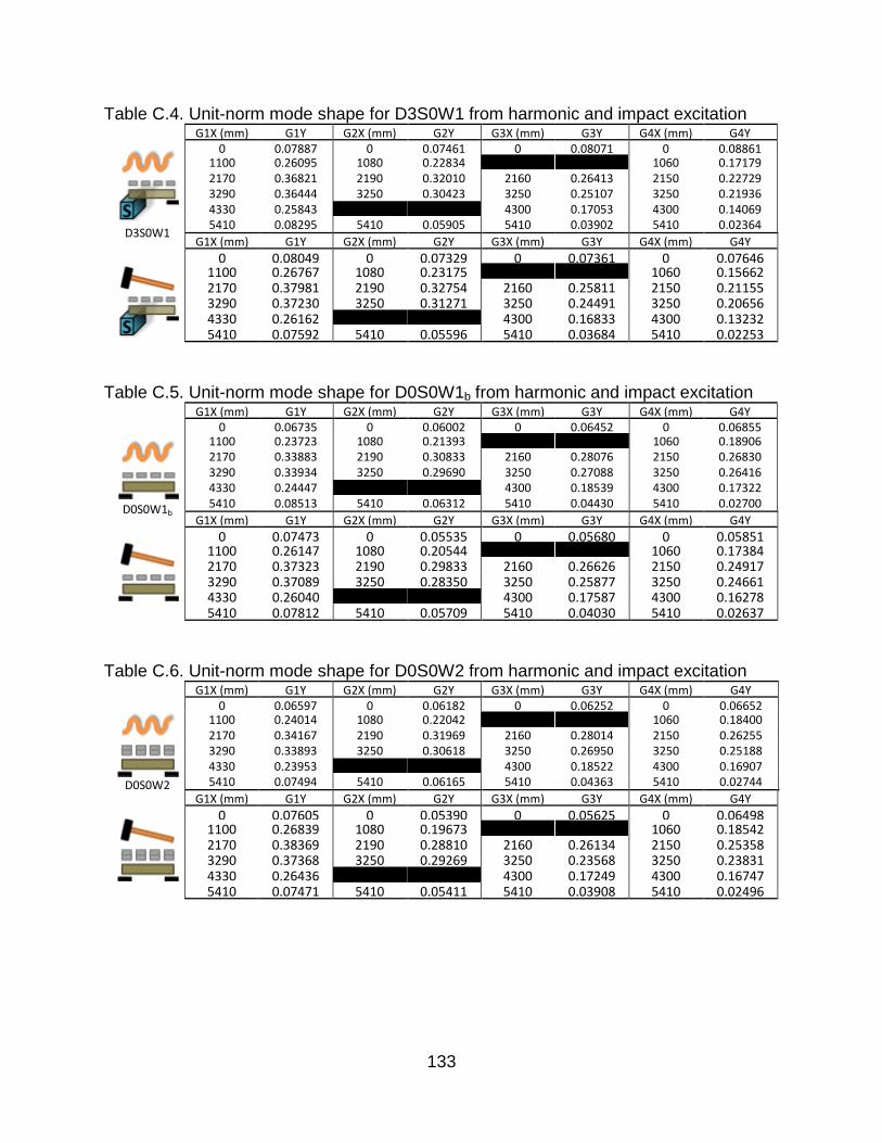
133


D3S0W1


1100 0.26095 1080 0.22834 1060 0.17179 2170 0.36821 2190 0.32010 2160 0.26413 2150 0.22729 3290 0.36444 3250 0.30423 3250 0.25107 3250 0.21936 4330 0.25843 4300 0.17053 4300 0.14069 5410 0.08295 5410 0.05905 5410 0.03902 5410 0.02364


0 0.08049 0 0.07329 0 0.07361 0 0.07646 1100 0.26767 1080 0.23175 1060 0.15662 2170 0.37981 2190 0.32754 2160 0.25811 2150 0.21155 3290 0.37230 3250 0.31271 3250 0.24491 3250 0.20656 4330 0.26162 4300 0.16833 4300 0.13232 5410 0.07592 5410 0.05596 5410 0.03684 5410 0.02253


D0S0W1b


1100 0.23723 1080 0.21393 1060 0.18906 2170 0.33883 2190 0.30833 2160 0.28076 2150 0.26830 3290 0.33934 3250 0.29690 3250 0.27088 3250 0.26416 4330 0.24447 4300 0.18539 4300 0.17322 5410 0.08513 5410 0.06312 5410 0.04430 5410 0.02700


0 0.07473 0 0.05535 0 0.05680 0 0.05851 1100 0.26147 1080 0.20544 1060 0.17384 2170 0.37323 2190 0.29833 2160 0.26626 2150 0.24917 3290 0.37089 3250 0.28350 3250 0.25877 3250 0.24661 4330 0.26040 4300 0.17587 4300 0.16278 5410 0.07812 5410 0.05709 5410 0.04030 5410 0.02637


D0S0W2


1100 0.24014 1080 0.22042 1060 0.18400 2170 0.34167 2190 0.31969 2160 0.28014 2150 0.26255 3290 0.33893 3250 0.30618 3250 0.26950 3250 0.25188 4330 0.23953 4300 0.18522 4300 0.16907 5410 0.07494 5410 0.06165 5410 0.04363 5410 0.02744


0 0.07605 0 0.05390 0 0.05625 0 0.06498 1100 0.26839 1080 0.19673 1060 0.18542 2170 0.38369 2190 0.28810 2160 0.26134 2150 0.25358 3290 0.37368 3250 0.29269 3250 0.23568 3250 0.23831 4330 0.26436 4300 0.17249 4300 0.16747 5410 0.07471 5410 0.05411 5410 0.03908 5410 0.02496

134


D4S0W1a


1100 0.24337 1080 0.22295 1060 0.20706 2170 0.31411 2190 0.29521 2160 0.28612 2150 0.28990 3290 0.30160 3250 0.27847 3250 0.27344 3250 0.28646 4330 0.21086 4300 0.19113 4300 0.19836 5410 0.06728 5410 0.05976 5410 0.05572 5410 0.04946


0 0.11144 0 0.09550 0 0.08535 0 0.07343 1100 0.25222 1080 0.22726 1060 0.19155 2170 0.33182 2190 0.30517 2160 0.28301 2150 0.27031 3290 0.32059 3250 0.28455 3250 0.26526 3250 0.26820 4330 0.22189 4300 0.18758 4300 0.18484 5410 0.06638 5410 0.05904 5410 0.05371 5410 0.04506


D4S0W2


1100 0.23824 1080 0.22168 1060 0.21071 2170 0.30911 2190 0.29765 2160 0.29024 2150 0.30068 3290 0.29591 3250 0.28122 3250 0.27723 3250 0.28723 4330 0.20385 4300 0.19307 4300 0.20435 5410 0.05940 5410 0.05653 5410 0.05395 5410 0.04814


0 0.12455 0 0.09226 0 0.07004 0 0.05382 1100 0.28962 1080 0.22781 1060 0.15676 2170 0.38224 2190 0.30801 2160 0.25150 2150 0.22517 3290 0.36084 3250 0.29165 3250 0.23797 3250 0.23093 4330 0.25037 4300 0.16934 4300 0.15817 5410 0.06816 5410 0.05578 5410 0.04620 5410 0.03746

Table C.9. Unit-norm mode shape for D0S0W1c from harmonic and impact excitation

D0S0W1c


0 0.07602 0 0.06207 0 0.06148 0 0.05985 1100 0.24737 1080 0.21622 1060 0.18433 2170 0.34625 2190 0.30866 2160 0.28012 2150 0.26731 3290 0.33950 3250 0.29521 3250 0.27061 3250 0.26412 4330 0.23478 4300 0.18455 4300 0.17831 5410 0.06382 5410 0.05115 5410 0.04256 5410 0.03354


0 0.07300 0 0.05967 0 0.05716 0 0.05481 1100 0.25411 1080 0.21912 1060 0.17139 2170 0.36178 2190 0.31696 2160 0.27463 2150 0.24769 3290 0.35374 3250 0.30400 3250 0.26263 3250 0.24453 4330 0.24419 4300 0.18037 4300 0.16590 5410 0.06170 5410 0.04996 5410 0.03996 5410 0.02938

135


D4S0W1b


0 0.09985 0 0.08621 0 0.08076 0 0.07339 1100 0.24296 1080 0.22059 1060 0.19833 2170 0.32507 2190 0.30079 2160 0.28158 2150 0.28045 3290 0.31582 3250 0.28543 3250 0.27084 3250 0.27804 4330 0.22328 4300 0.19077 4300 0.19202 5410 0.07400 5410 0.06288 5410 0.05491 5410 0.04630


0 0.09656 0 0.08306 0 0.07611 0 0.06680 1100 0.24882 1080 0.22357 1060 0.18486 2170 0.33862 2190 0.30925 2160 0.27854 2150 0.26159 3290 0.33027 3250 0.29618 3250 0.26804 3250 0.26018 4330 0.23152 4300 0.18703 4300 0.18079 5410 0.07236 5410 0.06160 5410 0.05255 5410 0.04191


D5S0W1


0 0.09038 0 0.07433 0 0.07223 0 0.06978 1100 0.24905 1080 0.21844 1060 0.19094 2170 0.33852 2190 0.30344 2160 0.28141 2150 0.27298 3290 0.32901 3250 0.28994 3250 0.27084 3250 0.27027 4330 0.22645 4300 0.18612 4300 0.18519 5410 0.06316 5410 0.05136 5410 0.04719 5410 0.04304


0 0.08979 0 0.07291 0 0.06626 0 0.06001 1100 0.26210 1080 0.22421 1060 0.16846 2170 0.36334 2190 0.31639 2160 0.26999 2150 0.24099 3290 0.35220 3250 0.30359 3250 0.25708 3250 0.23967 4330 0.24407 4300 0.17899 4300 0.16233 5410 0.06745 5410 0.05335 5410 0.04323 5410 0.03521


D6S0W1


0 0.11194 0 0.09479 0 0.08763 0 0.07945 1100 0.25606 1080 0.22863 1060 0.19567 2170 0.33702 2190 0.30610 2160 0.27958 2150 0.27072 3290 0.32215 3250 0.28605 3250 0.26474 3250 0.26461 4330 0.22312 4300 0.18078 4300 0.17740 5410 0.06546 5410 0.05166 5410 0.04273 5410 0.03474


0 0.10844 0 0.09253 0 0.08291 0 0.07153 1100 0.26164 1080 0.23167 1060 0.18016 2170 0.35049 2190 0.31489 2160 0.27600 2150 0.25049 3290 0.33588 3250 0.29855 3250 0.26278 3250 0.24530 4330 0.23077 4300 0.17724 4300 0.16501 5410 0.06243 5410 0.05060 5410 0.04093 5410 0.03134

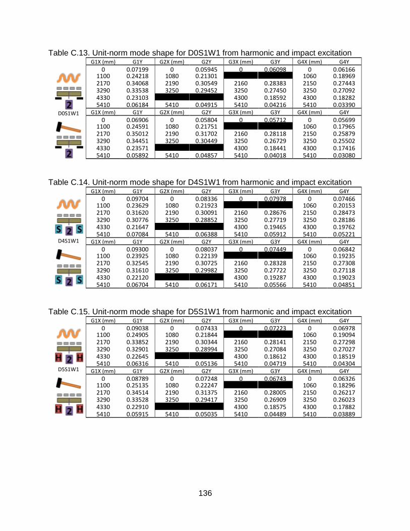
136


D0S1W1


0 0.07199 0 0.05945 0 0.06098 0 0.06166 1100 0.24218 1080 0.21301 1060 0.18969 2170 0.34068 2190 0.30549 2160 0.28383 2150 0.27443 3290 0.33538 3250 0.29452 3250 0.27450 3250 0.27092 4330 0.23103 4300 0.18592 4300 0.18282 5410 0.06184 5410 0.04915 5410 0.04216 5410 0.03390


0 0.06906 0 0.05804 0 0.05712 0 0.05699 1100 0.24591 1080 0.21751 1060 0.17965 2170 0.35012 2190 0.31702 2160 0.28118 2150 0.25879 3290 0.34451 3250 0.30449 3250 0.26729 3250 0.25502 4330 0.23571 4300 0.18441 4300 0.17416 5410 0.05892 5410 0.04857 5410 0.04018 5410 0.03080


D4S1W1


0 0.09704 0 0.08336 0 0.07978 0 0.07466 1100 0.23629 1080 0.21923 1060 0.20153 2170 0.31620 2190 0.30091 2160 0.28676 2150 0.28473 3290 0.30776 3250 0.28852 3250 0.27719 3250 0.28186 4330 0.21647 4300 0.19465 4300 0.19762 5410 0.07084 5410 0.06388 5410 0.05912 5410 0.05221


0 0.09300 0 0.08037 0 0.07449 0 0.06842 1100 0.23925 1080 0.22139 1060 0.19235 2170 0.32545 2190 0.30725 2160 0.28328 2150 0.27308 3290 0.31610 3250 0.29982 3250 0.27722 3250 0.27118 4330 0.22120 4300 0.19287 4300 0.19023 5410 0.06704 5410 0.06171 5410 0.05566 5410 0.04851


D5S1W1


0 0.09038 0 0.07433 0 0.07223 0 0.06978 1100 0.24905 1080 0.21844 1060 0.19094 2170 0.33852 2190 0.30344 2160 0.28141 2150 0.27298 3290 0.32901 3250 0.28994 3250 0.27084 3250 0.27027 4330 0.22645 4300 0.18612 4300 0.18519 5410 0.06316 5410 0.05136 5410 0.04719 5410 0.04304


0 0.08789 0 0.07248 0 0.06743 0 0.06326 1100 0.25135 1080 0.22247 1060 0.18296 2170 0.34514 2190 0.31375 2160 0.28005 2150 0.26217 3290 0.33528 3250 0.29417 3250 0.26909 3250 0.26023 4330 0.22910 4300 0.18575 4300 0.17882 5410 0.05915 5410 0.05035 5410 0.04489 5410 0.03889

137


D6S1W1


0 0.11633 0 0.09526 0 0.08473 0 0.07485 1100 0.24016 1080 0.22463 1060 0.20960 2170 0.30443 2190 0.29806 2160 0.29409 2150 0.30021 3290 0.28664 3250 0.28040 3250 0.28077 3250 0.29759 4330 0.19144 4300 0.19321 4300 0.20646 5410 0.04680 5410 0.04714 5410 0.05020 5410 0.05183


0 0.10957 0 0.09139 0 0.07979 0 0.06992 1100 0.23789 1080 0.22543 1060 0.20484 2170 0.30762 2190 0.30363 2160 0.29285 2150 0.29561 3290 0.29351 3250 0.28804 3250 0.28088 3250 0.29313 4330 0.19486 4300 0.19355 4300 0.20272 5410 0.04443 5410 0.04590 5410 0.04752 5410 0.04746


D0S2W1


0 0.07738 0 0.06118 0 0.05760 0 0.05433 1100 0.25226 1080 0.21759 1060 0.17827 2170 0.35349 2190 0.31285 2160 0.27799 2150 0.26101 3290 0.34604 3250 0.30102 3250 0.26820 3250 0.25336 4330 0.23802 4300 0.18074 4300 0.16910 5410 0.06176 5410 0.04895 5410 0.03940 5410 0.02914


0 0.07634 0 0.05810 0 0.05258 0 0.04732 1100 0.26350 1080 0.21768 1060 0.16034 2170 0.37465 2190 0.31834 2160 0.26855 2150 0.23559 3290 0.36558 3250 0.30977 3250 0.26034 3250 0.22871 4330 0.25031 4300 0.17435 4300 0.15326 5410 0.05911 5410 0.04695 5410 0.03672 5410 0.02565


D4S2W1


0 0.10851 0 0.08854 0 0.07887 0 0.06853 1100 0.24432 1080 0.22244 1060 0.19859 2170 0.31937 2190 0.30121 2160 0.28682 2150 0.28564 3290 0.30747 3250 0.28766 3250 0.27566 3250 0.27921 4330 0.21310 4300 0.19151 4300 0.19417 5410 0.06463 5410 0.05899 5410 0.05550 5410 0.05020


0 0.10696 0 0.08751 0 0.07428 0 0.06124 1100 0.25274 1080 0.22716 1060 0.18351 2170 0.33539 2190 0.31148 2160 0.28180 2150 0.26335 3290 0.32341 3250 0.29979 3250 0.26675 3250 0.26197 4330 0.22256 4300 0.18764 4300 0.18125 5410 0.06357 5410 0.05854 5410 0.05325 5410 0.04541

138


D5S2W1


0 0.09629 0 0.07805 0 0.07374 0 0.06875 1100 0.26721 1080 0.22469 1060 0.17153 2170 0.36504 2190 0.31242 2160 0.26915 2150 0.24010 3290 0.35480 3250 0.29807 3250 0.25803 3250 0.23201 4330 0.24713 4300 0.17428 4300 0.15555 5410 0.07286 5410 0.05534 5410 0.04400 5410 0.03357


0 0.09397 0 0.07609 0 0.06892 0 0.06056 1100 0.27042 1080 0.22855 1060 0.15899 2170 0.37448 2190 0.32205 2160 0.26433 2150 0.22601 3290 0.36171 3250 0.31242 3250 0.24577 3250 0.21809 4330 0.25167 4300 0.17273 4300 0.14651 5410 0.06894 5410 0.05406 5410 0.04176 5410 0.03101


D6S2W1


0 0.11336 0 0.09258 0 0.08221 0 0.07206 1100 0.24671 1080 0.22595 1060 0.20319 2170 0.31871 2190 0.30279 2160 0.28909 2150 0.29044 3290 0.30348 3250 0.28636 3250 0.27497 3250 0.28078 4330 0.20660 4300 0.18718 4300 0.19092 5410 0.05630 5410 0.04999 5410 0.04620 5410 0.04143


0 0.10990 0 0.08982 0 0.07698 0 0.06520 1100 0.25193 1080 0.22818 1060 0.19166 2170 0.33117 2190 0.31098 2160 0.28534 2150 0.27454 3290 0.31572 3250 0.29560 3250 0.27055 3250 0.26766 4330 0.21495 4300 0.18515 4300 0.18163 5410 0.05564 5410 0.04946 5410 0.04383 5410 0.03744

139

APPENDIX D. MODE SHAPE COMPONENTS

In this appendix, the average mode shape component values are listed in the tables.

The figures are plotted in the same manner as the bar chart described in Figure 4.20.

The results from harmonic excitation and impact excitation are both presented in this

appendix.

It should be noted, that in cases with negative differential substructure movement

(where the right support had a greater amplitude than the left support), the average

mode shape components (A, B and C) were scaled to add to unity.

140

Table D.1. Summary of average mode shape components from harmonic excitation

Damage Case

Mode Shape Component

Harmonic

A B C

Damage Case


Harmonic

A B C

D0S0W1a

0.73390 0.04564 0.22046

D0S0W1c

0.74153 0.04103 0.21744

D1S0W1

0.71215 0.08287 0.20499

D4S0W1b

0.67195 0.05848 0.26957

D2S0W1

0.65496 0.15115 0.19388

D5S0W1

0.70588 0.05657 0.23755

D3S0W1

0.69354 0.08284 0.22362

D6S0W1

0.67669 0.10335 0.21996

D0S0W1b

0.74175 0.02947 0.22878

D0S1W1

0.74683 0.04009 0.21308

D0S0W2

0.74056 0.03372 0.22572

D4S1W1

0.67069 0.05038 0.27893

D4S0W1a

0.65167 0.08494 0.26340

D5S1W1

0.70758 0.05882 0.23361

D4S0W2

0.67350 0.07860 0.24790

D6S1W1

0.67704 0.09943 0.22352

D0S2W1

0.75329 0.04291 0.20380

D4S2W1

0.67477 0.06457 0.26066

D5S2W1

0.69866 0.06780 0.23354

D6S2W1

0.68528 0.09402 0.22070

141

Figure D.1. Mode shape component amplitudes from harmonic excitation I

142

Figure D.2. Mode shape component amplitudes from harmonic excitation II

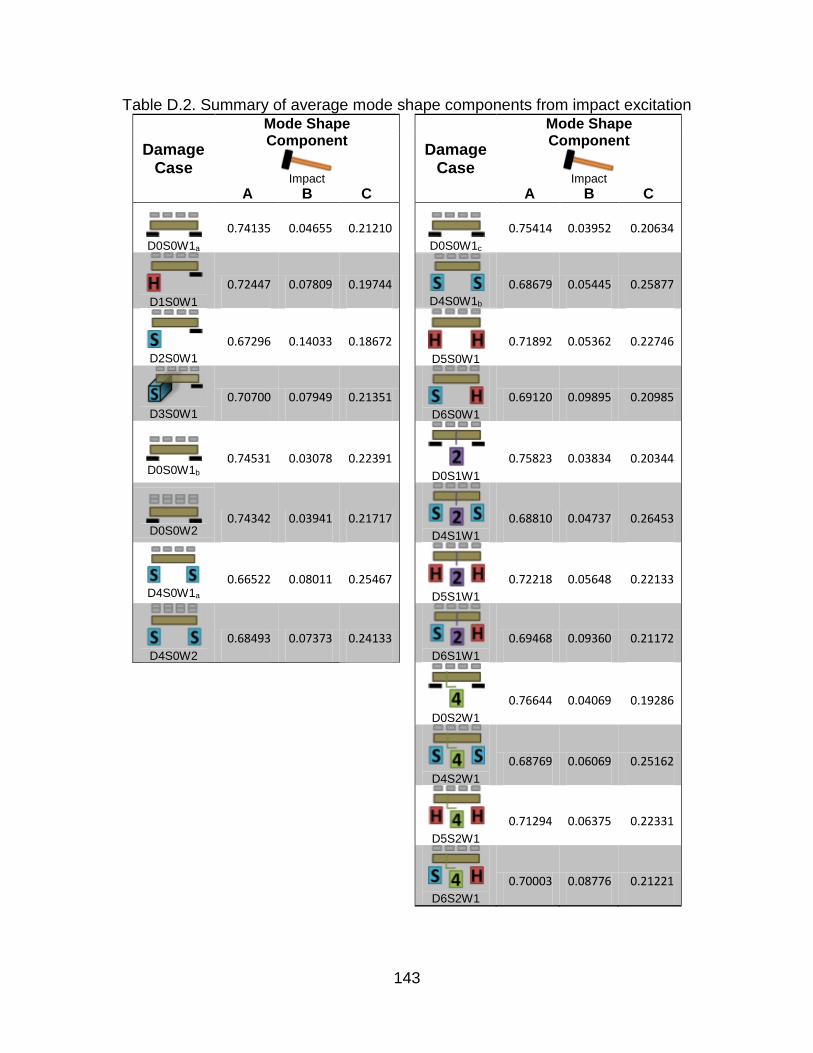
143

Table D.2. Summary of average mode shape components from impact excitation

Damage Case


Impact

A B C

Damage Case


Impact

A B C

D0S0W1a

0.74135 0.04655 0.21210

D0S0W1c

0.75414 0.03952 0.20634

D1S0W1

0.72447 0.07809 0.19744

D4S0W1b

0.68679 0.05445 0.25877

D2S0W1

0.67296 0.14033 0.18672

D5S0W1

0.71892 0.05362 0.22746

D3S0W1

0.70700 0.07949 0.21351

D6S0W1

0.69120 0.09895 0.20985

D0S0W1b

0.74531 0.03078 0.22391

D0S1W1

0.75823 0.03834 0.20344

D0S0W2

0.74342 0.03941 0.21717

D4S1W1

0.68810 0.04737 0.26453

D4S0W1a

0.66522 0.08011 0.25467

D5S1W1

0.72218 0.05648 0.22133

D4S0W2

0.68493 0.07373 0.24133

D6S1W1

0.69468 0.09360 0.21172

D0S2W1

0.76644 0.04069 0.19286

D4S2W1

0.68769 0.06069 0.25162

D5S2W1

0.71294 0.06375 0.22331

D6S2W1

0.70003 0.08776 0.21221

144

Figure D.3. Mode shape component amplitudes from impact excitation I

145

Figure D.4. Mode shape component amplitudes from impact excitation II

146

APPENDIX E. NATURAL FREQUENCIES

This appendix lists all the fundamental natural frequencies for the bridge states

considered in this thesis. Table E.1 lists the natural frequencies produced using

harmonic excitation, as well as impact loading. As stated in Section 3.5.2, harmonic

excitation produced more precise results (±0.05 Hz) than impact loading (±0.12 Hz).

147

Table E.1. Summary of all natural frequencies for timber bridge condition states

Damage Case

Natural frequency (Hz) Damage

Case


Harmonic ±0.05Hz

Impact ±0.12Hz

Harmonic ±0.05Hz

Impact ±0.12Hz

D0S0W1a

15.91 15.99 D0S0W1c

16.00 16.24

D1S0W1

15.82 15.99

D4S0W1b

15.44 15.63

D2S0W1

15.33 15.50

D5S0W1

15.77 15.99

D3S0W1

15.65 15.87

D6S0W1

15.44 15.69

D0S0W1b

15.85 16.08

D0S1W1

15.97 16.11

D0S0W2

15.02 15.30

D4S1W1

15.24 15.50

D4S0W1a

15.22 15.45

D5S1W1

15.60 15.76

D4S0W2

14.61 14.77

D6S1W1

15.26 15.50

D0S2W1

15.96 16.11

D4S2W1

15.22 15.38

D5S2W1

15.46 15.75

D6S2W1

15.35 15.50

148

APPENDIX F. VIBRATION-BASED DAMAGE DETECTION

The figures in this appendix include all the plots comparing an undamaged

superstructure bridge state to a damaged superstructure bridge state by considering

change in mode shape and change in curvature. Additionally, the figures consider a full

range of substructure states. In general, the substructure condition state had little effect

in the ability to detect superstructure damage. This conclusion is especially evident

when considering damage to Girder 4 (Figure F.9 to F.16).

Additionally, Table F.1 and Table F.2 provide the data used to establish the threshold

explained in Section 4.6.3 (Figure 4.34 Figure 4.35). In these tables, the mean and

standard deviation of the area under the change in mode shape vector (and area under

the change in curvature vector) were used when considering similar superstructure

bridge states to establish a threshold using a normal distribution (Z=3).

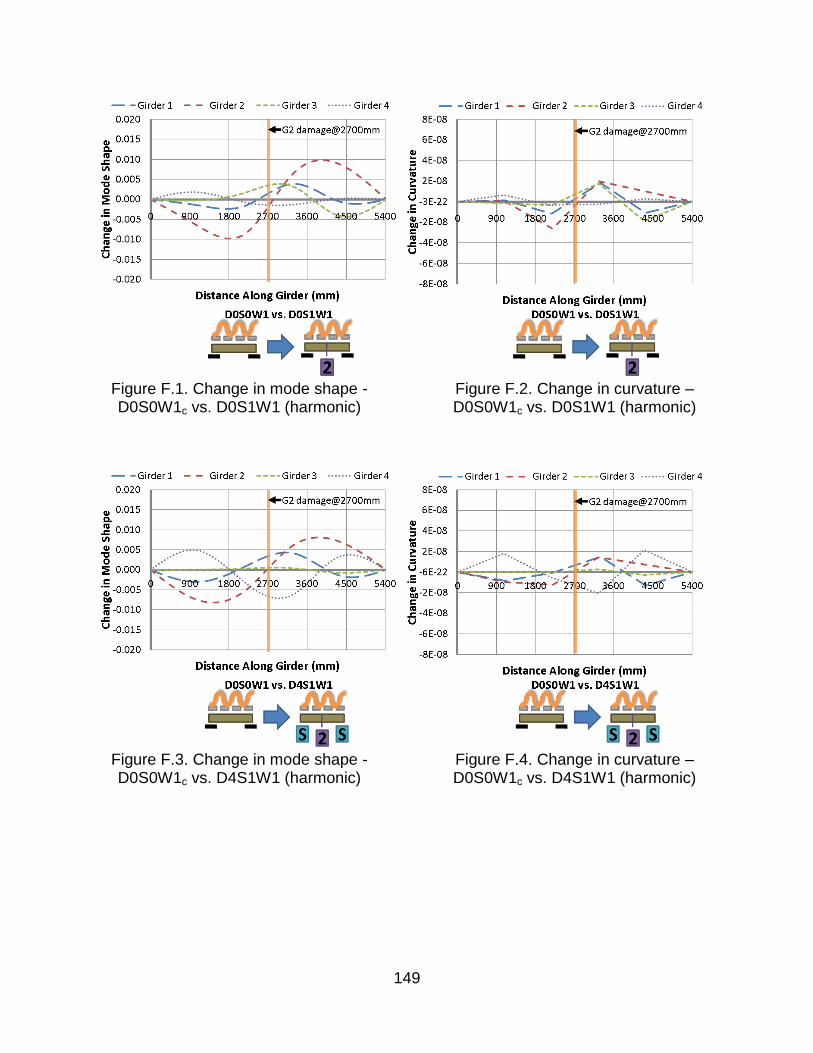
149

Figure F.1. Change in mode shape - D0S0W1c vs. D0S1W1 (harmonic)

Figure F.2. Change in curvature – D0S0W1c vs. D0S1W1 (harmonic)



150





151

Figure F.9. Change in mode shape -

D0S1W1 vs. D0S2W1 (harmonic) Figure F.10. Change in curvature – D0S1W1 vs. D0S2W1 (harmonic)



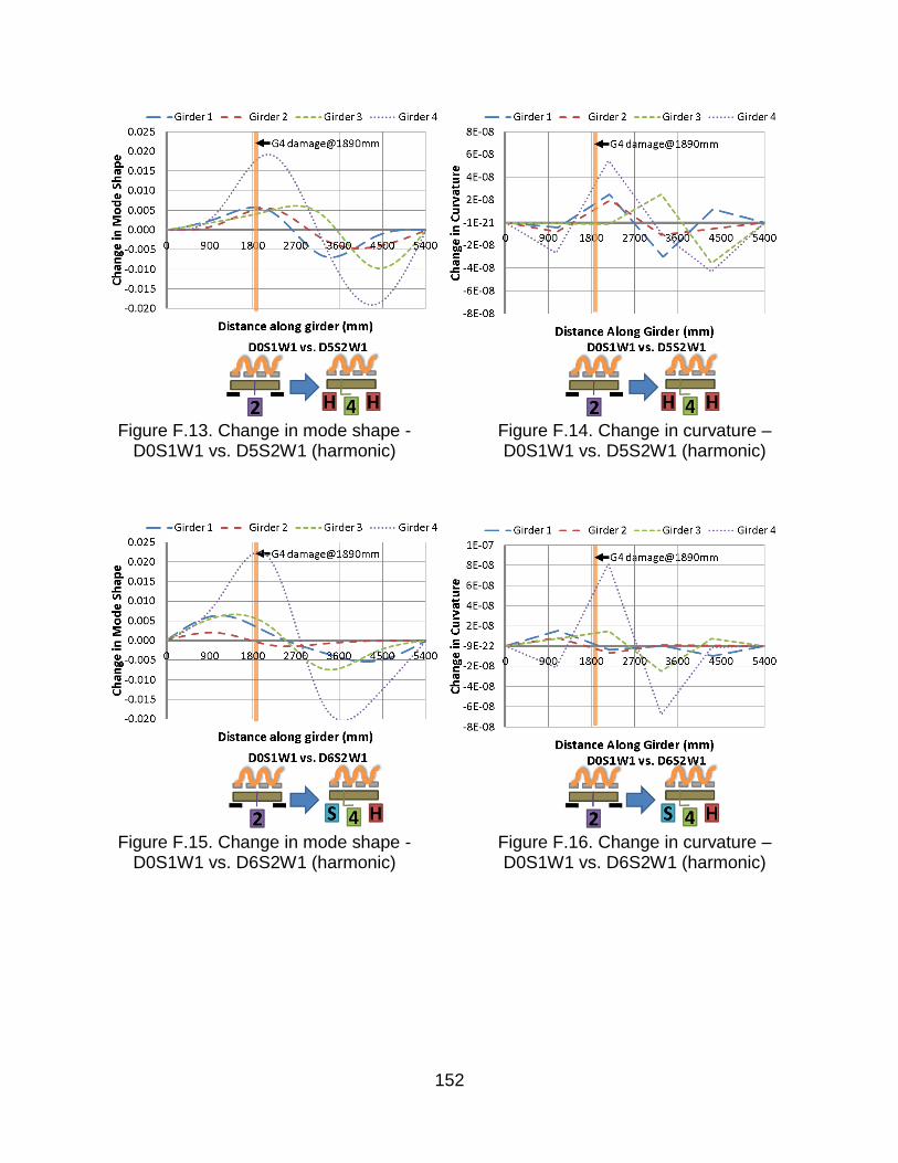
152





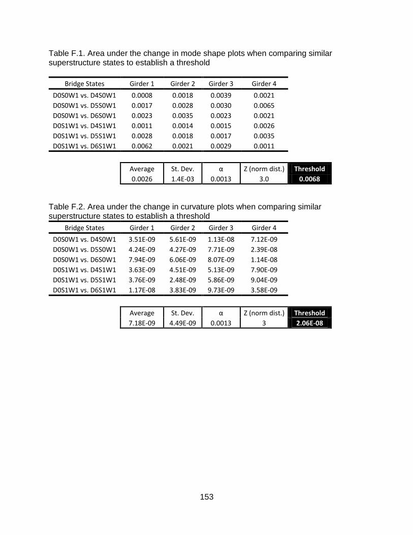
153

Table F.1. Area under the change in mode shape plots when comparing similar superstructure states to establish a threshold

Bridge States Girder 1 Girder 2 Girder 3 Girder 4 D0S0W1 vs. D4S0W1 0.0008 0.0018 0.0039 0.0021 D0S0W1 vs. D5S0W1 0.0017 0.0028 0.0030 0.0065 D0S0W1 vs. D6S0W1 0.0023 0.0035 0.0023 0.0021 D0S1W1 vs. D4S1W1 0.0011 0.0014 0.0015 0.0026 D0S1W1 vs. D5S1W1 0.0028 0.0018 0.0017 0.0035 D0S1W1 vs. D6S1W1 0.0062 0.0021 0.0029 0.0011

Average St. Dev. α Z (norm dist.) Threshold

0.0026 1.4E-03 0.0013 3.0 0.0068

Table F.2. Area under the change in curvature plots when comparing similar superstructure states to establish a threshold

Bridge States Girder 1 Girder 2 Girder 3 Girder 4 D0S0W1 vs. D4S0W1 3.51E-09 5.61E-09 1.13E-08 7.12E-09 D0S0W1 vs. D5S0W1 4.24E-09 4.27E-09 7.71E-09 2.39E-08 D0S0W1 vs. D6S0W1 7.94E-09 6.06E-09 8.07E-09 1.14E-08 D0S1W1 vs. D4S1W1 3.63E-09 4.51E-09 5.13E-09 7.90E-09 D0S1W1 vs. D5S1W1 3.76E-09 2.48E-09 5.86E-09 9.04E-09 D0S1W1 vs. D6S1W1 1.17E-08 3.83E-09 9.73E-09 3.58E-09

Average St. Dev. α Z (norm dist.) Threshold

7.18E-09 4.49E-09 0.0013 3 2.06E-08

154

APPENDIX G. STATISTICAL ANALYSIS

The statistical analysis was completed using Microsoft Excel 2007 with a two-sample t-

test assuming unequal variance (heteroscedastic t-test). The heteroscedastic t-test was

selected because of the distinct nature of the bridge cases considered; the

superstructure and substructure were both changing. In addition, the heteroscedastic t-

test accounts for unequal variances, which was observed throughout testing.

The two-sample F-test on variance was used to assess whether two bridge states had

equal variances by considering mode shape components. This test considered a two-

tailed probability with a hypothesis that the variances were not significantly different.

The means and standard deviations used to produce Tables G.1 to G.8 and G.10 are

presented in Table 5.1 Table 5.2 (for impact loadings). Table G.9 did not consider

individual girder responses and used the average mode shape components over the

four girders to describe a single bridge state. Other similar substructure condition states

were used to acquire a mean and standard deviation as indicated below:

D0 (rigid-rigid) D0S0W1c, D0S1W1, and D0S2W1

D4 (soft-soft) D4S0W1b, D4S1W1, and D4S2W1

D5 (hard-hard) D5S0W1, D5S1W1, and D5S2W1

D6 (soft-hard) D6S0W1, D6S1W1, and D6S2W1

155

i. Detection of Substructure Damage to a Single Support

Table G.1. T-test results considering bridge states with varying substructure stiffness under a single support H0: There is no difference in foundation stiffness

H1: There is a difference in foundation stiffness (if p<0.1, reject H0)

Bridge State P-Values (damage to a single support)

Impact

Harmonic

D0S0W1(a)

D1S0W1

D2S0W1

D3S0W1

D0S0W1(a)

A

1 0.550 0.066 0.117

B 0.019 0.000 0.441

C 0.621 0.427 0.969

D1S0W1

A 0.468

1 0.169 0.501

B 0.018 0.000 0.972

C 0.611 0.701 0.641

D2S0W1

A 0.059 0.171

1 0.273

B 0.000 0.000 0.197

C 0.425 0.707 0.462

D3S0W1

A 0.057 0.457 0.297

1 B 0.472 0.995 0.222

C 0.955 0.652 0.488

Excel function:

=ttest(array1,array2, 2 tails, heteroscedastic t-test)

array1 Girder 1; Girder 2; Girder 3; Girder 4

o Bridge state 1 using mode shape component (A,B or C)



156

ii. Detection of Local Substructure Damage

Table G.2. F-test on variance results considering bridge states with varying substructure stiffness under a single support H0: Both foundations have a uniform stiffness

H1: One of the foundations has a non-uniform stiffness (if p<0.1, reject H0)

Bridge State P-Values (damage to a single support)

Impact

Harmonic

D0S0W1(a)

D1S0W1

D2S0W1

D3S0W1

D0S0W1(a)

A

1 0.586 0.449 0.503

B 0.636 0.568 0.029

C 0.710 0.883 0.729

D1S0W1

A 0.440

1 0.826 0.238

B 0.715 0.921 0.012

C 0.736 0.822 0.477

D2S0W1

A 0.308 0.791

1 0.170

B 0.702 0.986 0.010

C 0.951 0.783 0.623

D3S0W1

A 0.602 0.210 0.139

1 B 0.025 0.013 0.012

C 0.566 0.370 0.526

Excel function:

=ftest(array1,array2)





157

iii. Substructure Damage Detection on Both Supports

Table G.3. T-test results considering bridge states with varying substructure stiffness under both supports H0: There is no difference in foundation stiffness


Bridge State P-Values (damage to both supports)

Impact

Harmonic

D0S0W1(c)

D4S0W1(b)

D5S0W1

D6S0W1

D0S0W1(c)

A

1 0.006 0.002 0.004

B 0.302 0.350 0.009

C 0.051 0.314 0.875

D4S0W1(b)

A 0.009

1 0.057 0.781

B 0.196 0.921 0.001

C 0.071 0.150 0.060

D5S0W1

A 0.009 0.090

1 0.065

B 0.315 0.859 0.002

C 0.407 0.211 0.383

D6S0W1

A 0.010 0.816 0.116

1 B 0.005 0.001 0.009

C 0.922 0.093 0.485

Excel function:






158

iv. Influence of Superimposed mass

Table G.4. T-test results considering bridge states with varying substructure stiffness and superimposed mass H0: There is no difference in foundation stiffness


Bridge State P-Values (influence of superimposed mass)

Impact

Harmonic

D0S0W1(b)

D0S0W2

D4S0W1(a)

D4S0W2

D0S0W1(b)

A

1 0.868 0.005 0.024

B 0.807 0.116 0.157

C 0.895 0.355 0.567

D0S0W2

A 0.567

1 0.006 0.025

B 0.917 0.211 0.286

C 0.995 0.299 0.476

D4S0W1(a)

A 0.012 0.011

1 0.365

B 0.174 0.154 0.617

C 0.294 0.265 0.298

D4S0W2

A 0.040 0.026 0.379

1 B 0.215 0.197 0.554

C 0.498 0.467 0.337

Excel function:






159

v. Superstructure Damage Detection

Table G.5. T-test results considering bridge states with similar substructure stiffness (D0) and varying superstructure states H0: There is no difference in foundation stiffness


Bridge State P-Values

Impact

Harmonic

D0S0W1(c)

D0S1W1

D0S2W1

D0S0W1(c)

A

1 0.499 0.171

B 0.945 0.939

C 0.895 0.544

D0S1W1

A 0.574

1 0.321

B 0.954 0.878

C 0.858 0.619

D0S2W1

A 0.344 0.572

1 B 0.898 0.856

C 0.594 0.712




Impact

Harmonic

D4S0W1(b)

D4S1W1

D4S2W1

D4S0W1(b)

A

1 0.929 0.961

B 0.205 0.592

C 0.752 0.681

D4S1W1

A 0.946

1 0.981

B 0.096 0.275

C 0.664 0.251

D4S2W1

A 0.899 0.841

1 B 0.602 0.260

C 0.652 0.217

160




Impact

Harmonic

D5S0W1

D5S1W1

D5S2W1

D5S0W1

A

1 0.665 0.399

B 0.718 0.462

C 0.658 0.815

D5S1W1

A 0.844

1 0.202

B 0.835 0.555

C 0.827 0.897

D5S2W1

A 0.382 0.247

1 B 0.517 0.551

C 0.863 0.997




Impact

Harmonic

D6S0W1

D6S1W1

D6S2W1

D6S0W1

A

1 0.848 0.668

B 0.807 0.317

C 0.913 0.895

D6S1W1

A 0.987

1 0.813

B 0.871 0.798

C 0.863 0.964

D6S2W1

A 0.717 0.740

1 B 0.446 0.832

C 0.972 0.801

For Table G.5 to G.8 the Excel function used was the same as previous student‟s t-

tests.

161

Since the above four tables show no significant difference between superstructure

states, the mode shape components from the four girders were averaged together. The

following table compares substructure response, while using the average girder

response to produce three similar substructure states.

Table G.9. T-test results considering bridge states with varying substructure stiffness and varying superstructure states H0: There is no difference in foundation stiffness


Bridge State P-Values (damage to both supports)

Impact

Harmonic

D0W1

S0/S1/S2

D4W1

S0/S1/S2

D5W1

S0/S1/S2

D6W1

S0/S1/S2

D0W1

S0/S1/S2

Avg A

1 0.002 0.001 0.000

Avg B 0.058 0.021 0.003

Avg C 0.001 0.017 0.123

D4W1

S0/S1/S2

Avg A 0.001

1 0.007 0.091

Avg B 0.052 0.485 0.002

Avg C 0.001 0.004 0.005

D5W1

S0/S1/S2

Avg A 0.001 0.003

1 0.004

Avg B 0.024 0.577 0.001

Avg C 0.020 0.017 0.011

D6W1

S0/S1/S2

Avg A 0.000 0.109 0.003

1 Avg B 0.001 0.002 0.001

Avg C 0.123 0.009 0.002

Excel function:


array1 S0;S1;S2

o Bridge state 1 using averaged mode shape component (A,B or C) of the

four girders

array2 S0;S1;S2

o Bridge state 2 using averaged mode shape component (A,B or C) of the

four girders

162

vi. Practical Application

Table G.10. T-test results considering bridge states with varying substructure stiffness under a single support using the limited accelerometer configuration H0: There is no difference in foundation stiffness


P-Values (for reduced sensors)

Impact

Harmonic

D0S0W1(a)

D1S0W1

D2S0W1

D3S0W1

D0S0W1(a)

A

1 0.570 0.068 0.129

B 0.017 0.000 0.441

C 0.616 0.408 0.985

D1S0W1

A

N/A 1 0.177 0.528

B 0.000 0.992

C 0.683 0.656

D2S0W1

A

N/A N/A 1 0.260

B 0.184

C 0.464

D3S0W1

A

N/A N/A N/A 1 B

C

Excel function:






VIBRATION-BASED DAMAGE DETECTION FOR TIMBER BRIDGES

Documents

Transcript of VIBRATION-BASED DAMAGE DETECTION FOR TIMBER BRIDGES