Finite Element Modeling for Vibration Analysis of Shell Membrane

by

Sai Sudharsanan Paranjothy

1

TABLE OF CONTENTS

ABSTRACT: ..................................................................................................................................................... 2

1.INTRODUCTION: ......................................................................................................................................... 3

2. MODELING AND MATERIALS:.................................................................................................................... 3

3. ANALYSIS SETUP: ...................................................................................................................................... 4

4. CONVERGENCE STUDIES: .......................................................................................................................... 5

5. THEORETICAL SOLUTIONS: ........................................................................................................................ 6

6. RESULTS AND DISCUSSION: ...................................................................................................................... 7

7. CONCLUSION: ............................................................................................................................................ 9

8. REFERENCES: ............................................................................................................................................. 9

APPENDIX: ................................................................................................................................................... 10

I. CALCULATION OF NATURAL FREQUENCIES (ANALYTICAL SOLUTION) : .............................................. 10

II. TABLE A) VALUES OF CONSTANTS ��� FOR DIFFERENT VALUES OF n AND s .................................... 11

III. TABLE B): VALUES OF NATURAL FREQUENCIES FOR DIFFERENT TENSION VALUES .......................... 11

IV. MODELS FOR VARYING NUMBER OF ELEMENTS 12,21,45 AND 87 : ............................................... 11

V. MODE SHAPES AND STRESS DISTRIBUTION FOR OTHER FREQUENCIES: ........................................... 12

VI. FREQUENCY RESULT SUMMARY FOR SHELL 181: .............................................................................. 13

VII. STIFFNESS , MASS AND LOAD MATRICES CALCULATED FOR ONE ELEMENT ALONG RADIUS: ......... 14

VII. DERIVATION OF ANALYTICAL SOLUTION: ......................................................................................... 16

2

ABSTRACT:

The study reviews the natural frequencies and mode shapes of transverse vibrations pre-stressed steel membrane through finite element analysis and correlates the results with analytical solutions. The natural frequencies of first two modes of vibration for the first two harmonics of the membrane, simply supported at its radius were obtained. Analyses were performed with ANSYS with two different choice of 4-noded bilinear shell elements. Convergence studies were carried out to obtain the optimal number of elements for the particular size of the membrane. The effect of pre-stress on the natural frequencies were studied .The modal displacement shapes were compared with the available mathematical solution obtained by solving the governing differential equations.

3

1.INTRODUCTION:

The most important parameters governing designs of dynamically loaded structures are natural frequencies and mode shapes. They are also important for Power Spectral Density analyses, transient or harmonic modal superposition analyses. The problem chosen to study is a circular membrane of radius 5 inches and thickness .00005 inches, simply supported at its radius.Shell41 and Shell181 membrane elements were used to model the problem under varying assumptions on behavior. Membrane action had to be taken into account considering the ratio between thickness and radius. Prestress plays an important role in determining the natural frequency. A body force in the form of uniform temperature is applied to induce prestress, static solution is run and then modal analysis was carried out. The mathematical solution for displacements are in the form of Bessel function of first order. Results obtained by finite element software are compared with analytical and mathematical solutions and results are validated. Convergence studies are carried out to increase accuracy with optimum number of elements. The results and their physical significance are then studied in detail.

The frequency equation of a continuous system yields infinite number of natural frequencies and modes, and in contrast with discrete systems, we have to incorporate boundary conditions to deduce the same. If frequencies are denoted by pns, where n is the mode and s is the harmonic, n also stands for the number of nodal diameters and s stands for the number of nodal circles(interchangeably used with λnm with subscripts standing for the same). Nodal circles and nodal diameters are formed by points which remain stationary in the vibration cycle.

2. MODELING AND MATERIALS:

A 30o sector of the circular membrane was modeled using shell41 elements for the first trial. The nodes and elements were directly modeled without generating meshes from area , that in turn aided in careful control over the number of elements for convergence studies. The nodes were created and were rotated in the polar co-ordinate system to obtain a sector of nodes, and then individual elements were defined over them. A cyclic expansion extrapolated the results over the entire circular domain.Shell41, or the membrane shell, has only the membrane stiffness and no bending stiffness. The element selection is warranted because an assumption of negligible bending stiffness is used in theory of in-plane transverse vibration of membranes. However, Shell 181 elements with both membrane and bending stiffness were used in a latter trial to validate the assumption. A uniform body force was applied in the form of temperature by applying fixed constraints to all the nodes. The induced prestress is dictated by the relation S = E αt (∆T).The material used is steel and the loading conditions and properties are as follows: E = 30 x 106 psi υ = 0.3 ρ = 0.00073 lb-sec2/in4

α = 1 x 10-5 in/in-°F

4

a = 5 in t = 0.00005 in S = 0.2 lb/in For the required prestress to be applied uniformly, a body force in temperature ,∆T = -13.3332°F was applied on all the nodes, by constraining them in all the directions. Later, while proceeding modal analysis, only the nodes along the radial boundary were constrained in the x and y direction , the membrane being in the xy plane and displacements along z were allowed.

3. ANALYSIS SETUP:

The equation solved during modal analysis is of the form:

a) ([ K]- pns2[M ]) { ϕ}= 0

where ϕ stands for the circular mode shapes. To induce prestress, a uniform load of 0.2lb/inch was applied. Thus, a linear analysis for [K][u]=F is solved during the static solution, the stress stiffness matrix [S] is calculated from the stresses [σ] and is added to the stiffness matrix of vibration analysis. Thus the modified equation becomes

b) ([ K+S]- pns

2[M ]) { ϕ}= 0

In modal analysis Block Lanczos method was used to extract four modes in the range of 1 to 1000Hz. Similar procedure was repeated for 12, 21, 90 and 140 elements to model a 30o sector and convergence studies were made. Shown below is the model of 72 elements, with simply supported constraints along radius and cyclic symmetry on the other edges of the sector. Models for other number of elements are shown in appendix.

Figure 1. Simply supported model of 72 Elements

5

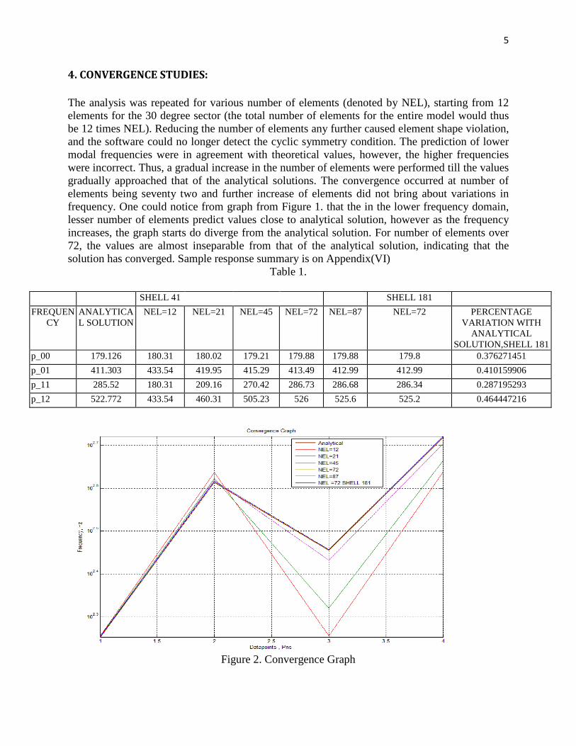
4. CONVERGENCE STUDIES:

The analysis was repeated for various number of elements (denoted by NEL), starting from 12 elements for the 30 degree sector (the total number of elements for the entire model would thus be 12 times NEL). Reducing the number of elements any further caused element shape violation, and the software could no longer detect the cyclic symmetry condition. The prediction of lower modal frequencies were in agreement with theoretical values, however, the higher frequencies were incorrect. Thus, a gradual increase in the number of elements were performed till the values gradually approached that of the analytical solutions. The convergence occurred at number of elements being seventy two and further increase of elements did not bring about variations in frequency. One could notice from graph from Figure 1. that the in the lower frequency domain, lesser number of elements predict values close to analytical solution, however as the frequency increases, the graph starts do diverge from the analytical solution. For number of elements over 72, the values are almost inseparable from that of the analytical solution, indicating that the solution has converged. Sample response summary is on Appendix(VI)

Table 1.

SHELL 41 SHELL 181

FREQUENCY

ANALYTICAL SOLUTION

NEL=12 NEL=21 NEL=45 NEL=72 NEL=87 NEL=72 PERCENTAGE VARIATION WITH

ANALYTICAL SOLUTION,SHELL 181

p_00 179.126 180.31 180.02 179.21 179.88 179.88 179.8 0.376271451

p_01 411.303 433.54 419.95 415.29 413.49 412.99 412.99 0.410159906

p_11 285.52 180.31 209.16 270.42 286.73 286.68 286.34 0.287195293

p_12 522.772 433.54 460.31 505.23 526 525.6 525.2 0.464447216

Figure 2. Convergence Graph

6

5. THEORETICAL SOLUTIONS:

In accordance with the textbook, "Vibration Problems in Engineering" by S.Timoshenko, the frequency can be deduced by substituting a function of the form Z=a1cos(πr/2a)+a2cos(3πr/2a)..., in ritz approximation for deflection v=Zcos(pt-α), where r is the radial distance of the point in consideration. Substituting the deflections in potential and kinetic energy, the frequency was obtained as ( refer Appendix VIII for derivations)

c) ��� =��√ �

�

where S is the uniform tension per unit length of the boundary, w is the weight of the membrane per unit area and a is the radius of the membrane. The constant ��� is determined by the table shown in Appendix.

d) p�� =�.���

�√���.�����.�

�.������^��

=1.7914 Hz

Analytical solution calculations for other frequencies are shown in appendix. The values are tabulated in Table 1. and FEM solutions were found to be in a good agreement with the same, with a maximum variation of 0.4%.

The exact solution for displacements and frequency can be found out by solving the differential equation

e) where,

T = Tension / unit length

ρ = Density

The mathematical solution is of the form:

f) where, λnm = frequencies Jn = Bessel function of order one αnm and βnm = constants.

7

For t=0, the ratio of the frequencies λ01/λ02 =0. 43569*a ,is a constant , which gives the radius of first modal circle. This analytical solution gives the first modal circle to occur at 2.18 inches and the FEM Solution of 2.14 inches is in good agreement with the same.

6. RESULTS AND DISCUSSION:

As predicted by the mathematical solution for wave differential equation, the first harmonic of the 0th mode, corresponding to frequency p01 has the deflection plot in the shape of a standing wave, reaching its maximum at the centre and gradually dying out at the ends. This fundamental mode has no nodal diameters but one circular mode, called modal circle. The acoustic significance of the membrane exhibiting this mode of vibration is it transmits sound very effectively, acting like a monopole source. Since it dissipates its vibrational energy in the form of radiated acoustic energy, it comes to rest very soon. The second harmonic of the 0th mode, corresponding to frequency p02 has two nodal circles and no nodal diameters. One nodal circle occurs near the outer edge and the other at a value close to 0.436*a, according to the mathematical solution. The maximum stress is for p02 frequency and the value is 1767.7 psi (refer Appendix V). The first harmonic of the first mode, corresponding to frequency p11 has one nodal circle near the edge and one nodal diameter across the centre. The second harmonic of the first mode corresponding to frequency p12 has two nodal circles and one nodal diameter as predicted by the theoretical equations. A stress and the displacement plots of p12 for full view of the plate after cyclic expansion have been shown in Figures 2 & 3. The displacement plot of the plate in side view clearly shows the shape of a Bessel function of order one, Jn where n=1, corresponding to n in pns and stresses vary according to the direction of displacement. The stresses induced in the plate are symmetric and are of varying nature but of the same magnitude on opposite sides of the nodal diameter. The maximum stress in this mode is 1627.8 psi for prestress of 0.2 psi which is much lower than the yield stress of steel which is 36,000 psi. The typical prestress induced in membranes for industrial use are in the order of 10-100 N/m (0.057 lb/in to 0.57 lb/in). The natural frequencies for prestress values of 0.4 lb/in and 0.5 lb/in are studied with the same model and have been tabulated in Appendix(III). The variation of natural frequencies with increase in prestress are in accordance with theoretical predictions. It could be seen from table that the results produced for natural frequencies were comparable for Shell41 and Shell181 elements. Thus, the initial assumption of negligible bending stiffness in the case of in-plane transverse vibration is validated. As said earlier, Shell41 elements have no rotational degree of freedom, thus containing three degrees of freedom per node. The stiffness and mass matrix for a single shell element having three degrees of freedom per node have been shown in Appendix(VII)

8

Figure 3 and 4: Stress Distribution and Side view of deformed plate for p12

9

7. CONCLUSION:

Natural frequencies of the vibrating membrane in relation to various parameters were studied. Convergence analysis was carried out by varying the number of elements and optimum number of elements for an accurate solution was found to be 72. The choice of element was validated by repeating the analysis for different shell elements, Shell41 and Shell 181 with similar inputs, and comparable results were achieved. The displacement plots were obtained and were compared to the mathematical functions. The natural frequencies increased almost linearly as the prestress induced was increased.

8. REFERENCES:

1. "Vibration Problems in Engineering" ,by S.Timoshenko.

2."Introduction to Finite Element Vibration Analysis", by Petyt.

3."Mechanical Vibrations", by S.S. Rao.

4. "FEM for Shells and Plates", presentation by Dr.Vikas Tomar.

10

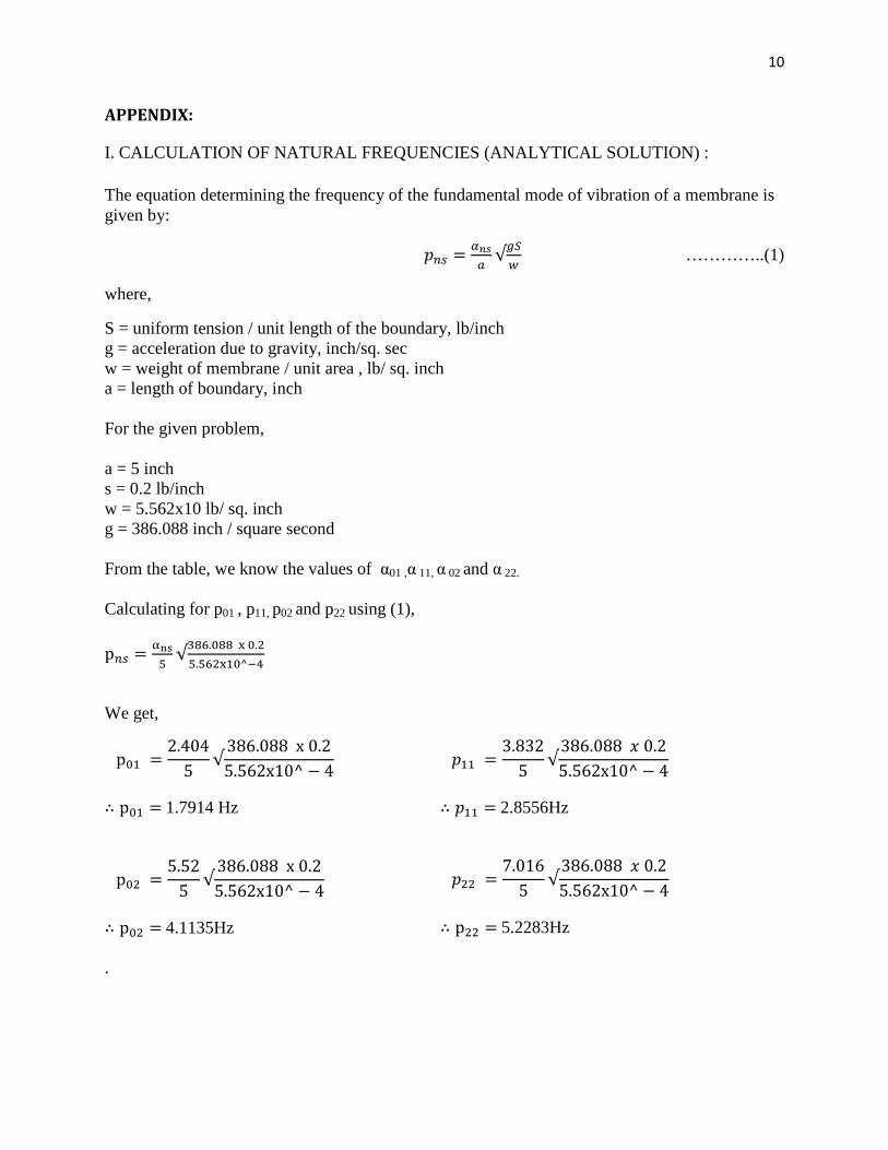
APPENDIX:

I. CALCULATION OF NATURAL FREQUENCIES (ANALYTICAL SOLUTION) :

The equation determining the frequency of the fundamental mode of vibration of a membrane is given by:

��� =��√ �

� …………..(1)

where,

S = uniform tension / unit length of the boundary, lb/inch g = acceleration due to gravity, inch/sq. sec w = weight of membrane / unit area , lb/ sq. inch a = length of boundary, inch For the given problem, a = 5 inch s = 0.2 lb/inch w = 5.562x10 lb/ sq. inch g = 386.088 inch / square second From the table, we know the values of α01 ,α 11, α 02 and α 22. Calculating for p01 , p11, p02 and p22 using (1),

p�� =�� �√���.�����.�

�.������^��

We get,

p�� =2.404

5√386.088x0.2

5.562x10^ − 4

∴ p�� =1.7914 Hz

��� =3.832

5√386.088,0.2

5.562x10^ − 4

∴ ��� =2.8556Hz

p�� =5.52

5√386.088x0.2

5.562x10^ − 4

∴ p�� =4.1135Hz

��� =7.016

5√386.088,0.2

5.562x10^ − 4

∴ p�� =5.2283Hz

.

11

II. TABLE A) VALUES OF CONSTANTS ��� FOR DIFFERENT VALUES OF n AND s s n=0 n=1 n=2 n=3 n=4 n=5

1 2.404 3.832 5.135 6.379 7.586 8.78

2 5.52 7.016 8.417 9.76 11.064 12.339

3 8.654 10.173 11.62 13.017 14.373 15.7

4 11.792 13.323 14.796 16.224 17.616 18.982

5 14.931 16.47 17.96 19.41 20.827 22.22

6 18.071 19.616 21.117 22.583 24.018 25.431

7 21.212 22.76 24.27 25.749 27.2 28.628

8 24.353 25.903 27.421 28.909 30.371 31.813

III. TABLE B): VALUES OF NATURAL FREQUENCIES FOR DIFFERENT TENSION VALUES

PRESTRESS .4 lb/in .5 lb/in

p_01 254.27 284.41 p_02 584.48 653.76 p_11 405.29 453.33 p_12 743.51 831.2

IV. MODELS FOR VARYING NUMBER OF ELEMENTS 12,21,45 AND 87 : Zoom percentage varies

NEL=12 NEL=21

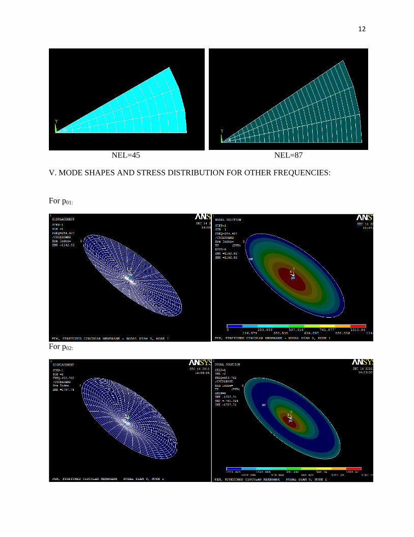
12

NEL=45 NEL=87

V. MODE SHAPES AND STRESS DISTRIBUTION FOR OTHER FREQUENCIES:

For p01:

For p02:

13

For p11

VI. FREQUENCY RESULT SUMMARY FOR SHELL 181: Repeated frequencies are to be ignored and only first two frequencies of load step one are considered. Additional frequencies are obtained due to the frequency range mentioned in anaysis being 1000.

14

VII. STIFFNESS , MASS AND LOAD MATRICES CALCULATED FOR ONE ELEMENT ALONG RADIUS:

15

16

VII. DERIVATION OF ANALYTICAL SOLUTION: