
VI. Determining the analysis of variance table
150
Statistical Modelling Chapter VI 1 VI. Determining the analysis of variance table VI.A The procedure VI.B The Latin square example VI.C Usage of the procedure VI.D Rules for determining the analysis of variance table — summary VI.E Determining the analysis of variance table — further examples
-
Upload
mckenzie-keller -
Category
Documents
-
view
16 -
download
0
description
VI. Determining the analysis of variance table. VI.AThe procedure VI.B The Latin square example VI.CUsage of the procedure VI.D Rules for determining the analysis of variance table — summary VI.E Determining the analysis of variance table — further examples. VI.AThe procedure. - PowerPoint PPT Presentation
Transcript of VI. Determining the analysis of variance table

Statistical Modelling Chapter VI 1
VI. Determining the analysis of variance table
VI.A The procedure
VI.B The Latin square example
VI.C Usage of the procedure
VI.D Rules for determining the analysis of variance table — summary
VI.E Determining the analysis of variance table — further examples

Statistical Modelling Chapter VI 2
VI.A The procedure
The 7 stepsa) Description of pertinent features of the studyb) The experimental structurec) Sources derived from the structure formulaed) Degrees of freedom and sums of squarese) The analysis of variance tablef) Maximal expectation and variation modelsg) The expected mean squares.• Should be done when designing an experiment
as it allows you to work out the properties of the experiment:
– in particular, what effects will occur in the experiment and how they will affect each other.

Statistical Modelling Chapter VI 3• Works for the vast majority of experimental designs used in practice.

Statistical Modelling Chapter VI 4
a) Description of pertinent features of the study
• The first stage in determining the analysis of variance table is to identify the following features:
1. observational unit
2. response variable
3. unrandomized factors
4. randomized factors
5. type of study

Statistical Modelling Chapter VI 5
Definitions of pertinent features• Definition VI.1: The observational unit is the native
physical entity which is individually measured.– For example, a person in a survey or a run in an experiment.
• Definition VI.2: The response variable is the measured variable that the investigator wants to see if the factors affect its response.– For example, the experimenter may want to determine whether or
not there are differences in yield, height, and so on for the different treatments — this is the response variable; that is, the variable of interest or for which differences might exist.
• Definition VI.3: The unrandomized factors are those factors that would index the observational units if no randomization had been performed.
• Definition VI.4: The randomized factors are those factors associated with the observational unit as a result of randomization.
• Definition VI.5: The type of study is the name of the experimental design or sampling method; for example, CRD, RCBD, LS, SRS, factorial, and so on.

Statistical Modelling Chapter VI 6
Unrandomized vs randomized factors
• To decide whether a factor is unrandomized or randomized, consider what information about the factors would be available if no randomization had been performed. – Unrandomized factors are innate to the observational units, so no
need to have performed the randomization to know which of their levels are associated with the different observational units.
– Levels of the randomized factors associated with the different observational units can only be known after the randomization has been performed.
• Rule VI.1: To determine whether a factor is unrandomized or randomized, ask the following question:– For an observational unit, can I identify the levels of that factor
associated with the unit if randomization has not been performed?
– If yes then the factor is unrandomized, if no then it is randomized.

Statistical Modelling Chapter VI 7
Features of experimentsExample VI.1 Calf diets• In an experiment to investigate differences between two calf diets the
progeny of five dams who had twins were taken.• For the two calves of each dam, one was chosen at random to
receive diet A and the other diet B. • The weight gained by each calf in the first 6 months was measured.• The observations for the experiment might be:
Observation
Dam
Calf
Diet
Weight Gain
1 1 1 A 125 2 1 2 B . 3 2 1 B . 4 2 2 A . 5 3 1 B . 6 3 2 A . 7 4 1 A . 8 4 2 B . 9 5 1 A . 10 5 2 B .

Statistical Modelling Chapter VI 9
Summary of the features of the study
1. Observational unit– A calf (10)
2. Response variable– Weight gain
3. Unrandomized factors– Dam, Calf
4. Randomized factors– Diet
5. Type of study– RCBD

Statistical Modelling Chapter VI 10
Unrandomized factors unique• Dam and Calf uniquely identify the observations
as no 2 observational units with the same combination of these two factors – (for example 2,1).
Observation
Dam
Calf
Diet
Weight Gain
1 1 1 A 125 2 1 2 B . 3 2 1 B . 4 2 2 A . 5 3 1 B . 6 3 2 A . 7 4 1 A . 8 4 2 B . 9 5 1 A . 10 5 2 B .

Statistical Modelling Chapter VI 11
Example VI.2 Plant yield
• Consider a CRD experiment consisting of 5 observations, each observation being the yield of a single plot which had one of three varieties applied to it.
• The results of the experiment are as follows:
• What are the features of the study?
Plot Variety Yield 1 A 213 2 C 256 3 A 225 4 B 183 5 B 201

Statistical Modelling Chapter VI 12
Features of plant experiment
1. Observational unit– a plotVariables (including factors) are?– Yield, Variety, Plot
2. Response variable– Yield
3. Unrandomized factors– Plot
4. Randomized factors– Variety
5. Type of study– CRD
• Note that two of the levels of the factor Variety are replicated twice and the third only once.

Statistical Modelling Chapter VI 13
Additional points
• Feature reflected in ANOVA table, particularly the unrandomized and randomized factors.
Source unrandomized Plots randomized Variety Residual
• The number of unrandomized factors is a characteristic of each design.

Statistical Modelling Chapter VI 14
Example VI.3 Pollution effects of petrol additives
• Consider the experiment to investigate the reduction in the emission of nitrous oxides resulting from the use of four different petrol additives.
• Four cars and four drivers are employed in this study with additives being assigned to a particular driver-car combination according to a Latin square.
Results for the 44 Latin square experiment
Car 1 2 3 4
I B 20
D 20
C 17
A 15
II A 20
B 27
D 23
C 26
Driver III D 20
C 25
A 21
B 26
IV C 16
A 16
B 15
D 13
(Additives: A, B, C, D)

Statistical Modelling Chapter VI 15
Features of pollution experiment
1. Observational unit– a car with a driver Variables (including factors) are?– Reduction, Driver, Car, Additive
2. Response variable– Reduction
3. Unrandomized factors– Driver, Car
4. Randomized factors– Additive
5. Type of study– Latin square

Statistical Modelling Chapter VI 16
Features of surveysExample VI.4 Vineyard sampling • A vineyard of 125 vines is sampled at random with 15
vines being selected at random and the yields measured.
• What are the features of the study?1. Observational unit
– a vine Variables (including factors) are?– Yield, Vines
2. Response variable– Yield
3. Unrandomized factors– Vines
4. Randomized factors– Not applicable
5. Type of study– Simple random sample

Statistical Modelling Chapter VI 17
Example VI.5 Smoking effect on blood cholesterol• Consider an observational study to investigate the effect
of smoking on blood cholesterol by observing 30 patients and recording whether they smoke tobacco and measuring their blood cholesterol. Suppose it happens that 11 patients smoke and 19 patients do not smoke.
• What are the features of the study? 1. Observational unit
– a patient Variables (including factors) are?– Blood cholesterol, Smoking, Patients
2. Response variable– Blood cholesterol
3. Unrandomized factors– Smoking, Patients
4. Randomized factors– Not applicable
5. Type of study– Survey

Statistical Modelling Chapter VI 18
Unrandomized vs randomized factors revisited• In determining the unrandomized and
randomized factors it is most important to distinguish between – randomization: random selection to assign – random sampling: random selection to observe a
fraction of a wholly observable population• It is not surprising that surveys do not contain
randomized factors, since they do not involve randomization.
• Remember the crucial question is: – If I take an observational unit, can I tell which level of
this factor is associated with that unit without doing the randomization?
– If yes then unrandomized, otherwise randomized.

Statistical Modelling Chapter VI 19
b) The experimental structure• Having determined the unrandomized and randomized
factors, one next determines the experimental structure.• Rule VI.2: Determine the experimental structure by
– describing the nesting and crossing relationships between the unrandomized factors in the experiment,
– describing the crossing and nesting relationships betweeni. the randomized factors, andii. (the randomized and the unrandomized factors, if any.)
• Nos of levels of factors placed in front of names of factors.
• Often step ii) not be required.– assume that the effects of the randomized factors are
approximately the same for each observational unit– so unrandomized and randomized factors can be treated as
independent.

Statistical Modelling Chapter VI 20
Crossing vs nesting• Definition VI.6: Two factors are
intrinsically nested if units with the same level of the nested factor, but different levels of the nesting factor, have no apparent characteristic in common.
• Definition VI.7: Two factors are intrinsically crossed if units with the same level of one factor, but different levels of the second factor, have a common characteristic associated with the first factor.

Statistical Modelling Chapter VI 21
ExamplesExample VI.6 Student height — unknown age
Student 1 2 3
Sex M y1 y2 y3
F y4 y5 y6 • Student (3 levels) is intrinsically nested within Sex (2 levels).
– Two Student 1s, have different Sex– However, apparently nothing in common, save inconsequentially
labelled with same no.
Example VI.7 Student height — known age Age 18 19 20
Sex M y1 y2 y3
F y4 y5 y6 • Two factors are intrinsically crossed because two 18 year-old
students, even though different sex, have in common that they are both 18.
• Suppose I have 6 heights for 3 students of each sex.
• Suppose I have 6 students indexed by – Sex, with 2 levels, and– Age, with 3 levels.

Statistical Modelling Chapter VI 22
Notation for factor relationships• Between two factors:
– a slash (‘/’) indicates that they are nested (nested factor on right).
– an asterisk (‘*’) indicates that they are crossed – a wedge (‘’) signifies all combinations of the two
factors – a plus (+) indicates they are to be considered
independently.
• Order (high to low) of precedence of operators in a structure formula is ‘’, ‘/’, ‘*’ and ‘+’.
• For example, the structure formula A * B / C is the same as A * ( B / C ).

Statistical Modelling Chapter VI 23
Example VI.1 Calf diets (continued) • The factors were designated:
3. Unrandomized factors – Dam, Calf4. Randomized factors – Diet
• So are the unrandomized factors nested?– Well, 'Do we have information that connects a calf from one
dam with any of the calves from another dam?'
Observation
Dam
Calf
Diet
Weight Gain
1 1 1 A 125 2 1 2 B . 3 2 1 B . 4 2 2 A . 5 3 1 B . 6 3 2 A . 7 4 1 A . 8 4 2 B . 9 5 1 A . 10 5 2 B .
• No. So they are nested.

Statistical Modelling Chapter VI 24
Example VI.1 Calf diets (continued)
• In fact, Calf is nested within Dam. • This is written symbolically as Dam/Calf.• Thus the experimental structure for this
experiment is:
Structure Formula unrandomized 5 Dam/2 Calf randomized 2 Diet

Statistical Modelling Chapter VI 25
Example VI.3 Pollution effects of petrol additives (continued)• The factors were designated:
3. Unrandomized factors – Driver, Car4. Randomized factors – Additive
• So are the unrandomized factors nested?– Well, 'Do we have information that connects one of the drivers
of a car with a driver from another car?'
• Yes, one of the 4 from each of the other cars is the same driver.
Results for the 44 Latin square experiment
Car 1 2 3 4
I B 20
D 20
C 17
A 15
II A 20
B 27
D 23
C 26
Driver III D 20
C 25
A 21
B 26
IV C 16
A 16
B 15
D 13
(Additives: A, B, C, D)

Statistical Modelling Chapter VI 26
Example VI.3 Pollution effects of petrol additives (continued)
• They are crossed.• This is written symbolically as Driver*Car. • Thus the experimental structure for this
experiment is:
Structure Formula unrandomized 4 Driver*4 Car randomized 4 Additive

Statistical Modelling Chapter VI 27
Respecting intrinsic crossing• In pollution experiment Drivers & Cars intrinsically crossed.• Consider following two designs for the experiment:
Car 1 2 3 4
I B A A B II A D C A Driver III D C D D IV C B B C
(Additives: A, B, C, D) • LS on left — each Additive once in each row and column
• RCBD, with Cars (columns) as blocks, on right. – Each additive is used in a car once and only once.– Same cannot be said of drivers.– Appropriate structure for this design would be Car/Driver.– Use if thought no driver differences – more Residual df
• Only LS respects intrinsic crossing by restricting randomization in both directions
Car 1 2 3 4
I B D C A II A B D C Driver III D C A B IV C A B D
(Additives: A, B, C, D)

Statistical Modelling Chapter VI 28
Crossing & nesting not just intrinsic• A factor will be nested within another either
because:– they are intrinsically nested
or– because the randomization employed requires that they
be so regarded.
• Hence, for two factors to be crossed requires that:– they are intrinsically crossed
and– that the randomization employed respects this
relationship.
• A Latin square respects the crossing of its two unrandomized factors, the RCBD does not.
Statistical Modelling Chapter VI 29
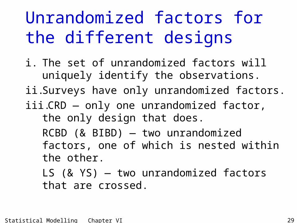
Unrandomized factors for the different designs
i. The set of unrandomized factors will uniquely identify the observations.
ii. Surveys have only unrandomized factors.
iii. CRD — only one unrandomized factor, the only design that does.
RCBD (& BIBD) — two unrandomized factors, one of which is nested within the other.
LS (& YS) — two unrandomized factors that are crossed.

Statistical Modelling Chapter VI 30
c) Sources derived from the structure formulae
• Having determined the experimental structure, the next step is to expand the formulae to obtain the sources that are to be included in the analysis of variance table.
• Rule VI.3: The rules for expanding structure formulae involving two factors A and B are:– A*B = A + B + A#B
where A#B represents the interaction of A and B– A/B = A + B[A]`where B[A] represents the nested effects of B within A
• More generally, if L and M are two formulae– L*M = L + M + L#M
where L#M is the sum of all pairwise combinations of a source in L with a source in M
– L/M = L + M[gf(L)]where gf(L) is the generalized factor (see definition VI.8 in section D, Degrees of freedom) formed from the combination of all factors in L.

Statistical Modelling Chapter VI 31
Examples
Example VI.1 Calf diets (continued)• Dam/Calf = Dam + Calf[Dam]
– where Calf[Dam] measures the difference between calves with the same Dam.
Example VI.3 Pollution effects of petrol additives (continued)
• Driver*Car = Car + Driver + Driver#Car– where Driver#Car measures extent to which Driver
differences change from Car to Car.
(More about interaction later.)

Statistical Modelling Chapter VI 32
d) Degrees of freedom and sums of squares
• The DFs for an ANOVA can be calculated with the aid of Hasse diagrams for Generalized-Factor Marginalities for each structure formula.
• Definition VI.8: A generalized factor is the factor formed from several (original) factors and whose levels are the combinations that occur in the experiment of the levels of the constituent factors.
• The generalized factor is the "meet" of the constituent factors and it is written as the list of constituent factors separated by "wedges" or "meets" ("").
• For convenience we include ordinary factors amongst the set of generalized factors for an experiment.
• Generalized factor corresponding to each source obtained from structure formulae —consists of the factors in source.

Statistical Modelling Chapter VI 33
Example VI.3 Pollution effects of petrol additives (continued)
• Consider sources Car and Driver#Car from Latin square example.
• The two generalized factors corresponding to these sources are Car and DriverCar
• DriverCar is a factor with 4 4 16 levels, one for each combination of Driver and Car.

Statistical Modelling Chapter VI 34
Marginality of generalized factors• Hasse diagram for Generalized-Factor Marginalities
displays marginality relationships between the generalized factors corresponding to the sources from a structure formula.
• Have previously discussed marginality for models.• Basically same here, except applies to generalized factors
that are potentially single indicator-variable terms in a model.
• Definition VI.9: One generalized factor, V say, is marginal to another, Z say, if the factors in the marginal generalized factor are a subset of those in the other and this will occur irrespective of the replication of the levels of the generalized factors.
• We write V Z.• Of course, a generalized factor is marginal to itself (V V).Example VI.3 Pollution effects of petrol additives
(continued)• Car is marginal to DriverCar (Car < DriverCar) as the
factor in Car is a subset of those in DriverCar.

Statistical Modelling Chapter VI 35
Constructing Hasse diagram• Rule VI.4: The Hasse diagrams for Generalized-Factor
Marginalities for a structure formula is formed by – placing generalized factors above those to which they are marginal – connecting them by an upwards arrow– adding each source alongside its generalized factor (to save
space use only 1st letter for each factor).
• In constructing a Hasse diagram,– The Universe factor (no named factor), connecting all units that
occurred in the experiment, is included at the top of the diagram.– Next consider generalized factors consisting of 1 factor, then 2
factors, and so on. Works because must be less factors in a marginal generalized factor.
• Under a generalized factor write its no. of levels. • Under a source write the DF for the corresponding source.
– Calculate as difference between the entry for its generalized factor and the sum of the DFs of all sources whose generalized factors are marginal to the current generalized factor.
Construct Hasse diagram for Dam/Calf and Driver*Car on board.

Statistical Modelling Chapter VI 37
DF when all factors in formula are crossed• Rule VI.5: When all the factors are crossed, the
degrees of freedom of any source can be calculated directly. The rule for doing this is:– For each factor in the source, calculate the number of
levels minus one and multiply these together.Example VI.3 Pollution effects of petrol
additives (continued)• Both Car and Driver in Latin square example
have 4 levels.• The degrees of freedom of Driver#Car,
corresponding to DriverCar, is (41)(41) 32 9.

Statistical Modelling Chapter VI 38
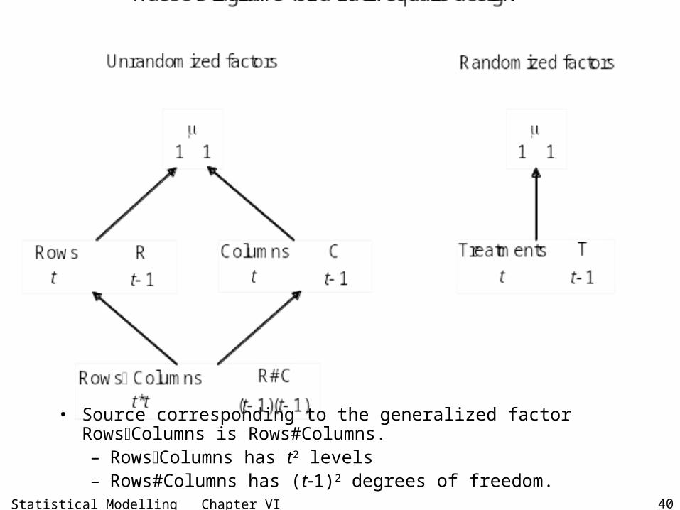
Hasse diagrams for some of the experiments

Statistical Modelling Chapter VI 39
• Source corresponding to generalized factor BlocksUnits is Units[Blocks]. – BlocksUnits has bt levels – Units[Blocks] has b(t1) degrees of freedom
Statistical Modelling Chapter VI 40
• Source corresponding to the generalized factor RowsColumns is Rows#Columns. – RowsColumns has t2 levels – Rows#Columns has (t1)2 degrees of freedom.

Statistical Modelling Chapter VI 41
Expression for Qs in terms of Ms• Clear can write SSq as Y'QY — but how to compute SSq• Need expression for Q in terms of Ms• Rule VI.6: There is a mean operator (M) and a quadratic-
form (Q) matrix for each generalized factor and source, respectively, obtained from the structure formulae.
• To obtain expressions for them, take the Hasse diagram of generalized factors for the formula: – for each generalized factor, replace its number of levels
combinations with its M matrix. – for each source, work out the expression for its Q matrix by
• taking the M matrix for its generalized factor; • subtract all expressions for Q matrices of sources whose
generalized factors are marginal to the generalized factor for the source whose expression you are deriving;
• replace the degrees of freedom under the source in the Hasse diagram with the expression.

Statistical Modelling Chapter VI 43
Example VI.3 Pollution effects of petrol additives (continued)

Statistical Modelling Chapter VI 44
Estimators of the quadratic forms or SSqs on which ANOVA based• YQDY, YQCY , YQDCY and YQAY• where
– QD MD MG
– QC MC MG
– QDC MDC MD MC + MG
– QA MA MG
• Note no YQGY• From this can say what vector to calculate for
forming SSq– e.g. YQDCY is the SSq of QDCY where
DC DC D C G Q Y M M M M Y Y D C G
• so element is? hence summation form of SSq is?

Statistical Modelling Chapter VI 45
Example VI.1 Calf diets (continued)
• Note use of "d" for Diet in contrast to "D" for Dam.• Thus estimators for SSqs are YQDY, YQDCY and YQdY• where QD MD MG, QDC MDC MD and Qd Md MG.

Statistical Modelling Chapter VI 46
e) The analysis of variance table
• At this step an analysis of variance table with the sources, their df and the quadratic-form estimators is formulated.
• Use following rule, although it only specifies the quadratic-form estimators for orthogonal experiments.
• Rule VI.7: The analysis of variance table is formed by: 1. Listing down all the unrandomized sources in the Source
column, and their degrees of freedom in the df column and the quadratic forms in the SSq column.
2. Then the randomized sources are placed indented under the unrandomized sources with which they are confounded, along with their df and, if the design is orthogonal, their quadratic forms.
3. Residual sources are added to account for the left-over portions of unrandomized sources and their dfs and quadratic forms are computed by difference.For orthogonal experiments, matrix of Residual quadratic form is the difference of the matrices of the quadratic forms from which it is computed.

Statistical Modelling Chapter VI 47
Example VI.1 Calf diets (continued)
and it can be proven that this matrix is symmetric and idempotent.
Source df SSq
unrandomized Dam 4
Calf[Dam] 5
DY Q Y
DCY Q Y
randomized Diet 1 dY Q Y
Residual 4 ResDCY Q Y
ResDC DC d DC dNow Y Q Y Y Q Y Y Q Y Y Q Q Y
ResDC DC dThat is Q Q Q

Statistical Modelling Chapter VI 48
Example VI.3 Pollution effects of petrol additives (continued)
and it can be proven that this matrix is symmetric and idempotent.
Source df SSq
unrandomized
Driver 3
Car 3
Driver#Car 9
CY Q Y
DY Q Y
DCY Q Y
randomized Additive 3 AY Q Y
Residual 6 ResDCY Q Y
ResDC DC AThat is Q Q Q
ResDC DC A DC ANow Y Q Y Y Q Y Y Q Y Y Q Q Y

Statistical Modelling Chapter VI 49
f) Maximal expectation and variation models
• Have been writing down expectation and variation models as the sum of a set of indicator-variable terms, these terms being derived from the generalized factors.
• Rule VI.8: To obtain the terms in the expectation and variation model:1. Designate each factor in the experiment as either fixed or
random.2. Determine whether a generalized factor is a potential expectation
or variation term as follows:– generalized factors that involve only fixed (original) factors are
potential expectation terms– generalized factors that contain at least one random (original) factor
will become variation terms.– If there is no unrandomized factor that has been classified as
random, the term consisting of all unrandomized factors will be designated as random.
3. The maximal expectation model is then the sum of all the expectation terms except those that are marginal to a term in the model; if there are no expectation terms, the model consists of a single term for the grand mean.
4. The maximal variation model is the sum of all the variation terms.

Statistical Modelling Chapter VI 50
Fixed versus random factors• So first step in determining model is to classify all the
factors in the experiment as fixed or random.• Definition VI.10: A factor will be designated as random if
it is anticipated that the distribution of effects associated with the population set of levels for the factor can be described using a probability distribution function.
• Definition VI.11: A factor will be designated as fixed if it is anticipated that a probability distribution function will not provide a satisfactory description the set of effects associated with the population set of levels for the factor.
• In practice– Random if
i. large number of population levels and ii. random behaviour
– Fixed if i. small or large number of population levels and ii. systematic or other non-random behaviour

Statistical Modelling Chapter VI 51
Fixed versus random (continued)
• Remember, must always model terms to which other terms have been randomized as random effects. – For example, because Treatments are randomized to
Units (within Blocks) in an RCBD, Units must be a random factor.
• It often happens, but not always, that:– unrandomized factors random factors so all terms
from unrandomized structure in variation modeland – randomized factors fixed factors so all terms from
randomized structure, minus marginal terms, in expectation model.

Statistical Modelling Chapter VI 55
• For Diet: random or fixed?– it is most unlikely that the 2 observed levels will be thought of as
being representative of a very large group of Diets and we anticipate that there will be arbitrary differences between the different Diets
and so it is a fixed factor.• For Dam: random or fixed?
– we can envisage a very large population of dams of which the 5 are representative and random dam differences so the set of population effects may well be described by a probability distribution
and so it is a random factor.• For Calf: random or fixed?
– similarly, a large population of calves and random calf differences so population effects described by probability distribution.
– anyway Diets randomized to Calf• Thus, appropriate to designate Dam and Calf as random
factors.• (diagnostic checking will try to support this assumption).
Example VI.1 Calf diets (continued)

Statistical Modelling Chapter VI 56
Formulating the model• The generalized factors in the experiment are:
– Dam, DamCalf and Diet.
• As the first two generalized factors contain at least one random factor, they are variation terms.
• The generalized factor Diet consists of only a fixed factor and so it is a potential expectation term.
• Hence, the maximal model to be used for this experiment is:– = E[Y] = Diet– V[Y] = Dam + DamCalf. – fixed = randomized and random = unrandomized

Statistical Modelling Chapter VI 57
g) The expected mean squares
Rule VI.9: The steps for constructing the E[MSQ]s for an orthogonal experiment are:
1. For each structure formula, take the Hasse diagram of generalized factors for the formula and, for each generalized factor F,
Under the corresponding source form the source's contribution to the E[MSQ]s by including
a) the expression on the left for every variation generalized factor V to which F is marginal (F < V), starting with the bottommost V and working up to F — that is the left hand expression for every V directly or indirectly connected to F from below — and
b) the expression under F.
Replace its no. of levels combinations, f, with a) if F is a term in the variation model, or
b) qF() if F is a potential expectation model term.
2Fn f

Statistical Modelling Chapter VI 58
Rule VI.9 (continued)2. Add contributions of unrandomized factors to E[MSq]s,
computed in the Hasse diagram, to the ANOVA table by putting each contribution against its source in the table, unless the source has been partitioned, in which case put the contribution against the sources into which it has been partitioned.
• When all the randomized factors are fixed, – unnecessary to use the Hasse diagram to work out the
contributions of their generalized factors to the E[MSq]s. – for each generalized factor, F, the contribution will be simply
qF() as no variation factors in diagrams. – just do the unrandomized factors using a Hasse diagram.
3. Repeat rule 2 for the other structure formula(e), adding the contributions to those already in the table. However, if a generalized factor occurs in more than one Hasse diagram, its or qF() is added only once.
2Fn f

Statistical Modelling Chapter VI 59
Example VI.1 Calf diets (continued)• So far
S o u r c e d f S S q D a m 4
C a l f [ D a m ] 5 DY Q Y
D CY Q Y
D ie t 1 dY Q Y
R e s id u a l 4 R e sD CY Q Y
• y = E[Y] = Diet• V[Y] = Dam + DamCalf.
• Work out E[MSq]

Statistical Modelling Chapter VI 60
VI.BThe Latin square exampleExample VI.3 Pollution effects of petrol additives
(continued)• We shall determine the E[MSq]s for Latin square
example.• Firstly, summarize what we have done so far.
Results for the 44 Latin square experiment
Car 1 2 3 4
I B 20
D 20
C 17
A 15
II A 20
B 27
D 23
C 26
Driver III D 20
C 25
A 21
B 26
IV C 16
A 16
B 15
D 13
(Additives: A, B, C, D)

Statistical Modelling Chapter VI 61
Summary of pollution experimenta) Description of pertinent features of the study
1. Observational unit — a car with a driver 2. Response variable
– Reduction
3. Unrandomized factors– Driver, Car
4. Randomized factors– Additive
5. Type of study– Latin square
b) The experimental structure
Structure Formula unrandomized 4 Driver*4 Car randomized 4 Additive

Statistical Modelling Chapter VI 62
Summary (continued)c) Sources derived from the structure formulae• Driver*Car = Driver + Car + Driver#Car• Additive = Additived) Degrees of freedom and sums of squares
Additives
MA Driver
MD Car MC
Driver Car
Unrandomized factors Randomized factors
MD MG
MDC MD MC+MG
MC MG MA MG
MG MG
MG MG
MDC
Hasse Diagrams for a petrol additive experiment
D C A
D#C
Additives
4 Driver
4 Car
4
Driver Car
Unrandomized factors Randomized factors
3
9
3 3
1 1
1 1
16
Hasse Diagrams for a petrol additive experiment
D C A
D#C

Statistical Modelling Chapter VI 63
Summary (continued)e) The analysis of variance table
Source df SSq Drivers 3 CY Q Y Cars 3
DY Q Y Drivers#Cars 9
DCY Q Y Additive 3
AY Q Y Residual 6
ResDCY Q Y
f) Maximal expectation and variation models • Take Cars and Drivers to be random and Additive to be
fixed — reasonable?• Then, referring to the Hasse diagram, the maximal
expectation and variation models are– = E[Y] = Additive and – var[Y] = Driver + Car + DriverCar

Statistical Modelling Chapter VI 64
Finishing upg)The expected mean squares• The expectation term is Additive.• The variation terms are:
– Driver, Car, and DriverCar.
• Hence, the variation components will be 2 2 2D C DC, and , respectively.
• In this experiment there are 16 observations and the values of f for Driver, Car, and DriverCar are 4, 4, and 16, respectively — see Hasse diagram.
• The multipliers of the components are:– 164 4, 164 4 and 1616 1, respectively.

Statistical Modelling Chapter VI 65
Hasse diagrams, with contributions to E[MSq]s
Source df SSq E[MSq] Car 3 CY Q Y Driver 3 DY Q Y
Driver#Car 9 DCY Q Y
Additive 3 AY Q Y
Residual 6 ResDCY Q Y
Total 15
DC D2 24
DC C2 24
2DC Aq ψ
DC2

Statistical Modelling Chapter VI 66
VI.C Usage of the procedure• Procedure should be carried at the design stage. • Can check the properties of the design that you propose
to use. – good idea to obtain a layout for the design in R and carry out an
analysis on randomly-generated data.
• Experimental structure central to this as it contains all the factors to be generated and the model formula will be of the form: Y ~ randomized structure
+ fixed unrandomized sources+ Error(unrandomized structure)
where Y is some randomly generated data.• Advantage is will provide a check
– are the sources, and where they occur in the analysis, what you expected?
– Are the degrees of freedom what you have calculated? – Are the correct F-tests being performed?

Statistical Modelling Chapter VI 67
VI.D Rules for determining the analysis of variance table
• A summary of the rules given in the notes

Statistical Modelling Chapter VI 68
VI.F Exercises
• Ex. VI.1-4 ask you to determine the ANOVA for experiments
• Ex. VI.5 asks you to obtain a randomized layout for Ex. VI.4 and a dummy analysis for it.

Statistical Modelling Chapter VI 69
VI.E Determining the analysis of variance table — further examples
• For each of the following studies determine the analysis of variance table (Source, df, SSq and E[MSq]) using the following seven steps:
a) Description of pertinent features of the study
b) The experimental structure
c) Sources derived from the structure formulae
d) Degrees of freedom and sums of squares
e) The analysis of variance table
f) Maximal expectation and variation models
g) The expected mean squares.

Statistical Modelling Chapter VI 70
Example VI.8 Mathematics teaching methods
• An educational psychologist wants to determine the effect of three different methods of teaching mathematics to year 10 students.
• Five metropolitan schools with three mathematics classes in year 10 are selected and the methods of teaching randomized to the classes in each school.
• After being taught by one of the methods for a semester, the average score of the students in a class is obtained.

Statistical Modelling Chapter VI 71
a) Description of pertinent features of the study
1. Observational unit – a class
2. Response variable– Test score
3. Unrandomized factors– Schools, Classes
4. Randomized factors– Methods
5. Type of study– An RCBD
b) The experimental structurec) Sources derived from the structure formulae

Statistical Modelling Chapter VI 72
d) Degrees of freedom and sums of squares
• Hasse diagrams for this study with – degrees of freedom– M and Q matrices

Statistical Modelling Chapter VI 73
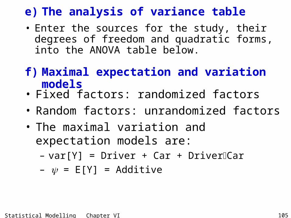
e) The analysis of variance table
• Enter the sources for the study, their degrees of freedom and quadratic forms, into the ANOVA table below.
• Fixed factors: randomized factor• Random factors: unrandomized factors• The maximal variation and expectation models
are:– Var[Y] – E[Y]
f) Maximal expectation and variation models

Statistical Modelling Chapter VI 74
g) The expected mean squares • The Hasse diagrams, with contributions to expected mean
squares, for this study are:

Statistical Modelling Chapter VI 75
ANOVA table with E[MSq]
Source df SSq E[MSq]
Schools 4 SYQY 2 2SC S3
Classes[Schools] 10 SCYQY
Methods 2 MYQY 2SC Mq
Residual 8 ResSCYQ Y 2
SC

Statistical Modelling Chapter VI 76
Example VI.9 Smoke emission from combustion engines
• A manufacturer of combustion engines is concerned about the percentage of smoke emitted by engines of a particular design in order to meet air pollution standards.
• An experiment was conducted involving engines with three timing levels, three throat diameters, two volume ratios in the combustion chamber, and two injection systems.
• Thirty-six engines designed to represent all combinations of these 4 factors — the engines were then operated in a completely random order so each engine was tested twice.
• The percent smoke emitted was recorded at each test.

Statistical Modelling Chapter VI 77
a) Description of pertinent features of the study
1. Observational unit – a test
2. Response variable– Percent Smoke Emitted
3. Unrandomized factors– Tests
4. Randomized factors– Timing, Diameter, Ratios, Systems
5. Type of study– Complete Four-factor CRD
Structure Formula unrandomized 72 Tests randomized 3 Timing*3 Diameter*2 Ratios*2 Systems
b) The experimental structure

Statistical Modelling Chapter VI 78
c) Sources derived from the structure formulae
Tests = Tests
Timing*Diameter*Ratios*Systems
= Timing + Diameter + Ratios + Systems
+ Timing#Diameter + Timing#Ratios
+ Timing#Systems + Diameter#Ratios
+ Diameter#Systems + Ratios#Systems
+ Timing#Diameter#Ratios
+ Timing#Diameter#Systems
+ Timing#Ratios#Systems
+ Diameter#Ratios#Systems
+ Timing#Diameter#Ratios#Systems

Statistical Modelling Chapter VI 79
d) Degrees of freedom and sums of squares
• To get degrees of freedom use rule for completely crossed structure.
• The degrees of freedom of a source is obtained by computing the number of levels minus one for each factor in the source and forming their product.
• Enter the sources for the study, their degrees of freedom and quadratic forms, into the ANOVA table below.
e) The analysis of variance table

Statistical Modelling Chapter VI 80
f) Maximal expectation and variation models
• Fixed factors: randomized factors • Random factors: unrandomized factors• The maximal variation and expectation models
are:– Var[Y] = Tests– = E[Y] = TimingDiameterRatiosSystems
• Expectation model consists of just generalized factor corresponding to source Timing#Diameter#Ratios#Systems; all other expectation generalized factors are marginal to this generalized factor.

Statistical Modelling Chapter VI 81
g) The expected mean squares
• In this case, using the Hasse diagrams to compute the E[MSq]s would be overkill.
• Since Tests is partitioned into the other sources in the table, this component occurs against all lines except Tests.
• All the randomized generalized factors are potential contributors to the expectation model and so their contributions to the E[MSq]s for the corresponding sources are of the form qF().
• There is one variation component 2 2t t
7272

Statistical Modelling Chapter VI 82
ANOVA table with E[MSq]
Source df SSq E[MSq]
Tests 71 tY Q Y
Timing 2 TY Q Y 2t Tq ψ
Diameter 2 DY Q Y 2t Dq ψ
Ratios 1 RY Q Y 2t Rq ψ
Systems 1 SY Q Y 2t Sq ψ
Timing#Diameter 4 TDY Q Y 2t TDq ψ
Timing#Ratios 2 TRY Q Y 2t TRq ψ
Timing#Systems 2 TSY Q Y 2t TSq ψ
Diameter#Ratios 2 DRY Q Y 2t DRq ψ
Diameter#Systems 2 DSY Q Y 2t DSq ψ
Ratios#Systems 1 RSY Q Y 2t RSq ψ
Timing#Diameter#Ratios 4 TDRY Q Y 2t TDRq ψ
Timing#Diameter#Systems 4 TDSY Q Y 2t TDSq ψ
Timing#Ratios#Systems 2 TRSY Q Y 2t TRSq ψ
Diameter#Ratios#Systems 2 DRSY Q Y 2t DRSq ψ
Timing#Diam#Ratios#System 4 TDRSY Q Y 2t TDRSq ψ
Residual 36 RestY Q Y 2
t

Statistical Modelling Chapter VI 83
Example VI.10 Lead concentration in hair
• An investigation was performed to discover trace metal concentrations in humans in the five major cities in Australia.
• The concentration of lead in the hair of fourth grade school boys was determined.
• In each city, 10 primary schools were randomly selected and from each school ten students selected. Hair samples were taken from the selected boys and the concentration of lead in the hair determined.

Statistical Modelling Chapter VI 84
a) Description of pertinent features of the study1. Observational unit
– hair of a boy
2. Response variable– Lead concentration
3. Unrandomized factors– Cities, Schools, Boys
4. Randomized factors– Not applicable
5. Type of study– A multistage survey
b) The experimental structurec) Sources derived from the structure formulae• Cities/Schools/Boys = (Cities + Schools[Cities])/Boys
= Cities + Schools[Cities]
+ Boys[gf(Cities + Schools[Cities])]
= Cities + Schools[Cities] + Boys[CitiesSchools]

Statistical Modelling Chapter VI 85
d) Degrees of freedom and sums of squares
• Hasse diagrams for this study with – degrees of freedom– M and Q matrices

Statistical Modelling Chapter VI 86
e) The analysis of variance table
• Enter the sources for the study, their degrees of freedom and quadratic forms, into the ANOVA table below.
• Fixed factors:• Random factors:• The maximal variation and expectation models
are:– Var[Y] – E[Y]
f) Maximal expectation and variation models

Statistical Modelling Chapter VI 87
g) The expected mean squares • The Hasse diagrams, with contributions to expected mean
squares, for this study are:

Statistical Modelling Chapter VI 88
ANOVA table with E[MSq]
Source df SSq E[MSq]
Cities 4 CY Q Y 2 2CSB CS C10 q
Schools[Cities] 45 CSY Q Y 2 2CSB CS10
Boys[Cities Schools] 450 CSBY Q Y 2CSB

Statistical Modelling Chapter VI 89
Example VI.11 Penicillin pain
• An experiment to investigate degree of pain experienced by patients when injected with penicillin of different potencies.
• There were 10 groups of three patients, all three patients being simultaneously injected with the same dose.
• Altogether 6 different potencies administered over 6 consecutive times; order randomized for each group.
• The total of the degree of pain experienced by the three patients was obtained, the pain for each patient having been measured on a five-point scale 0–4.

Statistical Modelling Chapter VI 90
a) Description of pertinent features of the study
1. Observational unit – A group of patients at a time
2. Response variable– Total pain score
3. Unrandomized factors– Group, Time
4. Randomized factors– Potency
5. Type of study– An RCBD
b) The experimental structurec) Sources derived from the structure formulae

Statistical Modelling Chapter VI 91
d) Degrees of freedom and sums of squares
• Hasse diagrams for this study with – degrees of freedom– M and Q matrices
(use g for Group to distinguish from G for Grand Mean)
Statistical Modelling Chapter VI 92
e) The analysis of variance table
• Enter the sources for the study, their degrees of freedom and quadratic forms, into the ANOVA table below.
• Fixed factors:• Random factors:• The maximal variation and expectation models
are:– Var[Y] – E[Y]
f) Maximal expectation and variation models

Statistical Modelling Chapter VI 93
g) The expected mean squares • The Hasse diagrams, with contributions to expected mean
squares, for this study are:

Statistical Modelling Chapter VI 94
ANOVA table with E[MSq]
Source df SSq E[MSq]
Groups 9 gY Q Y 2 2gT g6
Time[Groups] 50 gTY Q Y
Potencies 5 PY Q Y 2gT Pq ψ
Residual 45 ResgTY Q Y 2
gT
Total 59

Statistical Modelling Chapter VI 95
Example VI.12 Plant rehabilitation study
• In a plant rehabilitation study, the increase in height of plants of a certain species during a 12-month period was to be determined at three sites differing in soil salinity.
• Each site was divided into five parcels of land containing 4 plots and four different management regimes randomly assigned to the plots within a parcel.
• In each plot, six plants of the species were selected and marked and the total increase in height of all six plants measured.
• Note that the researcher is interested in seeing if any regime differences vary from site to site.

Statistical Modelling Chapter VI 96
a) Description of pertinent features of the study
1. Observational unit – a plot of plants
2. Response variable– Plant height increase
3. Unrandomized factors– Sites, Parcels, Plots
4. Randomized factors– Regimes
5. Type of study– A type of RCBD
b) The experimental structure
Structure Formula unrandomized 3 Sites/5 Parcels/4 Plots randomized 4 Regimes*Sites

Statistical Modelling Chapter VI 97
c) Sources derived from the structure formulae
• Sites/Parcels/Plots = Sites + Parcels[Sites]+ Plots[SitesParcels]
• Regimes*Sites = Regimes + Sites+ Regimes#Sites

Statistical Modelling Chapter VI 98
d) Degrees of freedom and sums of squares
• Hasse diagrams for this study with – degrees of freedom– M and Q matrices
(use L for Plots to distinguish from P for Parcels)

Statistical Modelling Chapter VI 99
e) The analysis of variance table
• Enter the sources for the study, their degrees of freedom and quadratic forms, into the ANOVA table below.
• Fixed factors:• Random factors:• The maximal variation and expectation models
are:– Var[Y] – E[Y]
f) Maximal expectation and variation models

Statistical Modelling Chapter VI 100
g) The expected mean squares • The Hasse diagrams, with contributions to
expected mean squares, for the unrandomized factors in this study are:
• Note that all the contributions of the randomized generalized factors will be of the form qF() as all the randomized factors are fixed.
Statistical Modelling Chapter VI 101
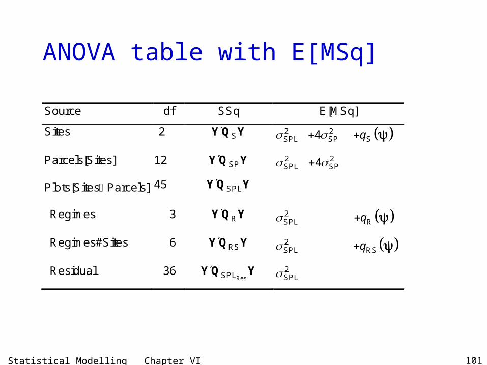
ANOVA table with E[MSq]
Source df SSq E[MSq]
Sites 2 SY Q Y 2 2SPL SP S4 q
Parcels[Sites] 12 SPY Q Y 2 2SPL SP4
Plots[Sites Parcels] 45 SPLY Q Y
Regimes 3 RY Q Y 2SPL Rq
Regimes#Sites 6 RSY Q Y 2SPL RSq
Residual 36 ResSPLY Q Y 2
SPL

Statistical Modelling Chapter VI 102
Example VI.13 Pollution effects of petrol additives
• Suppose a study is to be conducted to investigate whether four petrol additives differ in the amount by which they reduce the emission of oxides of nitrogen.
• Four cars and four drivers are to be employed in the study and the following Latin square arrangement is to be used to assign the additives to the driver-car combinations:
Car 1 2 3 4
I B D C A II A B D C Drivers III D C A B IV C A B D
(Additives A, B, C, D)

Statistical Modelling Chapter VI 103
a) Description of pertinent features of the study
1. Observational unit – a car with a driver
2. Response variable– Reduction
3. Unrandomized factors– Driver, Car
4. Randomized factors– Additive
5. Type of study– Latin square
b) The experimental structure
Structure Formula unrandomized 4 Driver*4 Car randomized 4 Additive

Statistical Modelling Chapter VI 104
c) Sources derived from the structure formulae
• Driver*Car = Driver + Car + Driver#Car• Additive = Additive
d) Degrees of freedom and sums of squares
Additives
MA Driver
MD Car MC
Driver Car
Unrandomized factors Randomized factors
MD MG
MDC MD MC+MG
MC MG MA MG
MG MG
MG MG
MDC
Hasse Diagrams for a petrol additive experiment
D C A
D#C
Additives
4 Driver
4 Car
4
Driver Car
Unrandomized factors Randomized factors
3
9
3 3
1 1
1 1
16
Hasse Diagrams for a petrol additive experiment
D C A
D#C
Statistical Modelling Chapter VI 105
e) The analysis of variance table
• Enter the sources for the study, their degrees of freedom and quadratic forms, into the ANOVA table below.
• Fixed factors: randomized factors• Random factors: unrandomized factors• The maximal variation and expectation models
are:– var[Y] = Driver + Car + DriverCar– = E[Y] = Additive
f) Maximal expectation and variation models

Statistical Modelling Chapter VI 106
g) The expected mean squares
• The Hasse diagrams, with contributions to expected mean squares, for this study are:

Statistical Modelling Chapter VI 107
ANOVA table with E[MSq]
Source df SSq E[MSq] Cars 3 CY Q Y DC D
2 24 Drivers 3 DY Q Y DC C
2 24
Drivers#Cars 9 DCY Q Y
Additives 3 AY Q Y 2DC Aq ψ
Residual 6 ResDCY Q Y DC
2
Total 15
Statistical Modelling Chapter VI 108
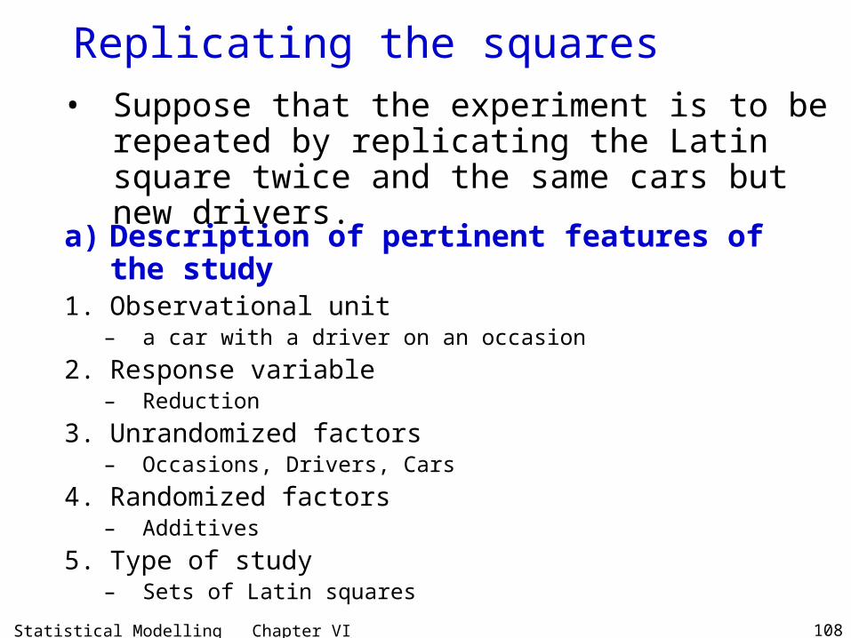
Replicating the squares
a) Description of pertinent features of the study1. Observational unit
– a car with a driver on an occasion
2. Response variable– Reduction
3. Unrandomized factors– Occasions, Drivers, Cars
4. Randomized factors– Additives
5. Type of study– Sets of Latin squares
• Suppose that the experiment is to be repeated by replicating the Latin square twice and the same cars but new drivers.

Statistical Modelling Chapter VI 109
b) The experimental structure
Structure Formula unrandomized (2 Occasions/4 Drivers)*4 Cars randomized 4 Additives
c) Sources derived from the structure formulae
(Occasions/Drivers)*Cars
= (Occasions + Drivers[Occasions])*Cars= Occasions + Drivers[Occasions] + Cars
+ Occasions#Cars + Drivers[Occasions]#Cars
Additives = Additives

Statistical Modelling Chapter VI 110
d) Degrees of freedom and sums of squares
• Hasse diagrams for this study with – degrees of freedom– M and Q matrices

Statistical Modelling Chapter VI 111
e) The analysis of variance table
• Enter the sources for the study, their degrees of freedom and quadratic forms, into the ANOVA table below.
• Fixed factors: randomized factors• Random factors: unrandomized factors• The maximal variation and expectation models
are:– var[Y] =– = E[Y] =
f) Maximal expectation and variation models

Statistical Modelling Chapter VI 112
g) The expected mean squares
• The Hasse diagrams, with contributions to expected mean squares, for the unrandomized factors in this study are:

Statistical Modelling Chapter VI 113
ANOVA table with E[MSq]
Source df SSq E[MSq]
Occasions 1 OY Q Y 2 2 2 2ODC OC OD O4 4 16
Dr[Occ] 6 ODY Q Y 2 2ODC OD4
Cars 3 CY Q Y 2 2 2ODC OC C4 8
Occ#Cars 3 OCY Q Y 2 2ODC OC4
Dr#Cars[Occ] 18 ODCY Q Y
Additives 3 AY Q Y 2ODC Aq ψ
Residual 15 ResODCY Q Y 2
ODC
Total 31

Statistical Modelling Chapter VI 114
Example VI.14 Controlled burning
• Suppose an environmental scientist wants to investigate the effect on the biomass of burning Areas of natural vegetation.
• There are available two Areas separated by several kilometres for use in the investigation.
• It is only possible to either burn or not burn an entire Area. The investigator randomly selects to burn one Area and the other Area is left unburnt as a control.
• She randomly samples 30 locations in each Area and measures the biomass at each location.

Statistical Modelling Chapter VI 115
a) Description of pertinent features of the study
1. Observational unit – a location
2. Response variable– Biomass
3. Unrandomized factors– Areas, Locations
4. Randomized factors– Burning
5. Type of study– a CRD with subsampling
b) The experimental structure
Structure Formula unrandomized 2 Areas/30 Locations randomized 2 Burning

Statistical Modelling Chapter VI 116
c) Sources derived from the structure formulae
• Areas/Locations = Areas + Locations[Areas]• Burning = Burning
d) Degrees of freedom and sums of squares

Statistical Modelling Chapter VI 117
e) The analysis of variance table
• Enter the sources for the study, their degrees of freedom and quadratic forms, into the ANOVA table below.
• Fixed factors: randomized factors• Random factors: unrandomized factors• The maximal variation and expectation models
are:– var[Y] = Areas + AreasLocations– = E[Y] = Burning
f) Maximal expectation and variation models

Statistical Modelling Chapter VI 118
g) The expected mean squares
• The Hasse diagrams, with contributions to expected mean squares, for this study are:

Statistical Modelling Chapter VI 119
ANOVA table with E[MSq]
Source df SSq E[MSq]
Areas 1 AY Q Y
Burning 1 BY Q Y 2 2AL A B30 q
Locations[Areas] 58 ALY Q Y 2AL
• We see that we cannot test for Burning differences because there is no source with expected mean square 2 2
AL A30
• The problem is that Burning and Area differences are totally confounded and cannot be separated.
• Shows in the ANOVA table derived using our approach.

Statistical Modelling Chapter VI 120
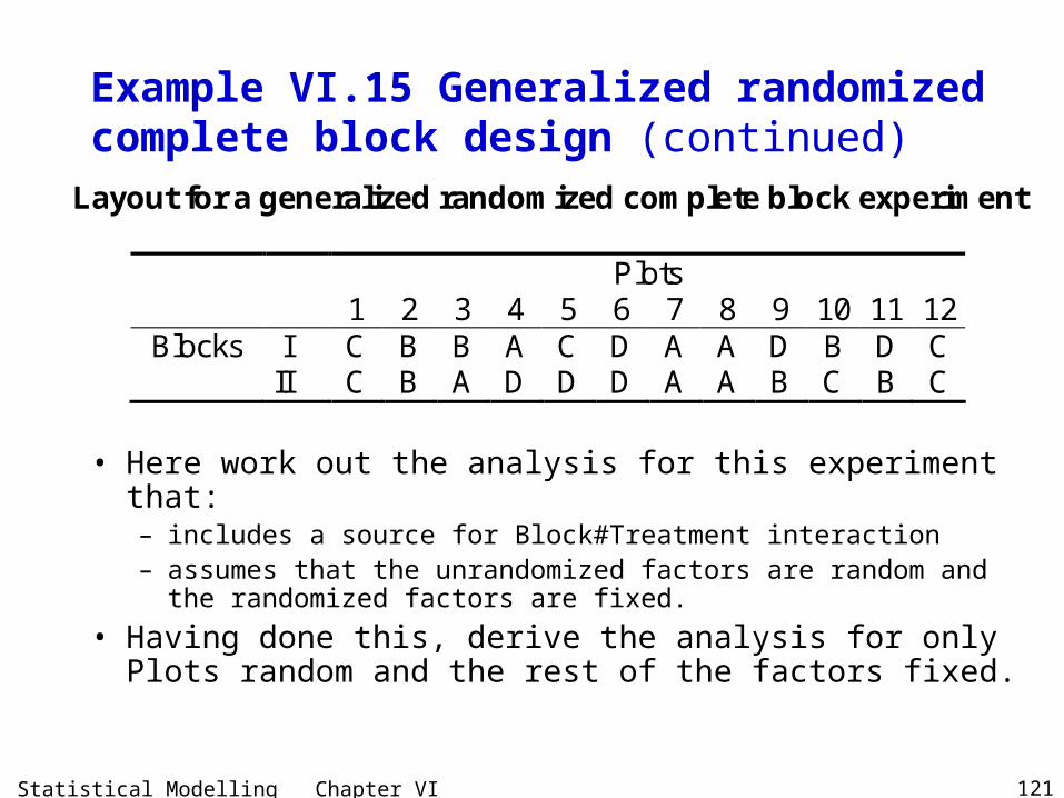
Example VI.15 Generalized randomized complete block design
• A generalized RCBD is the same as the ordinary RCBD, except that each treatment occurs more than once in a block — see section IV.G, Generalized randomized complete block design.
• For example, suppose four treatments are to be compared when applied to a new variety of wheat.
• I employed a generalized randomized complete block design with 12 plots in each of 2 blocks so that each treatment is replicated 3 times in each block.
• The yield of wheat from each plot was measured.
Statistical Modelling Chapter VI 121
Example VI.15 Generalized randomized complete block design (continued)
• Here work out the analysis for this experiment that:– includes a source for Block#Treatment interaction – assumes that the unrandomized factors are random and the
randomized factors are fixed.
• Having done this, derive the analysis for only Plots random and the rest of the factors fixed.
Layout for a generalized randomized complete block experiment
Plots 1 2 3 4 5 6 7 8 9 10 11 12
Blocks I C B B A C D A A D B D C II C B A D D D A A B C B C

Statistical Modelling Chapter VI 122
a) Description of pertinent features of the study
1. Observational unit – a plot
2. Response variable– Yield
3. Unrandomized factors– Blocks, Plots
4. Randomized factors– Treatments
5. Type of study– a Generalized Randomized Complete Block Design
b) The experimental structure
Structure Formula unrandomized 2 Blocks/12 Plots randomized 4 Treatments*Blocks

Statistical Modelling Chapter VI 123
c) Sources derived from the structure formulae
• Blocks/Plots = Blocks + Plots[Blocks]• Treatments*Blocks = Treatments + Blocks
+ Treatments#Blocks

Statistical Modelling Chapter VI 124
d) Degrees of freedom and sums of squares

Statistical Modelling Chapter VI 125
e) The analysis of variance table
• Enter the sources for the study, their degrees of freedom and quadratic forms, into the ANOVA table below.
• Fixed factors: randomized factors• Random factors: unrandomized factors• The maximal variation and expectation models
are:– var[Y] = BlocksPlots + TreatmentsBlocks – = E[Y] = Treatments
f) Maximal expectation and variation models

Statistical Modelling Chapter VI 126
g) The expected mean squares
• The Hasse diagrams, with contributions to expected mean squares, for this study are:

Statistical Modelling Chapter VI 127
ANOVA table with E[MSq]
Source df SSq E[MSq]
Blocks 1 BY Q Y 2 2 2BP BT B3 12
Plots[Blocks] 22 BPY Q Y
Treatments 3 TY Q Y 2 2BP BT T3 q
Treatments#Blocks 3 TBY Q Y 2 2BP BT3
Residual 16 ResBPY Q Y 2
BP
Total 23
• The denominator of the test for Treatments is Treatments#Blocks

Statistical Modelling Chapter VI 128
Only Plots random
• The maximal variation and expectation models are:– var[Y] = BlocksPlots– = E[Y] = TreatmentsBlocks
f) Maximal expectation and variation models

Statistical Modelling Chapter VI 129
ANOVA table with E[MSq]
Source df SSq E[MSq]
Blocks 1 BY Q Y 2BP Bq
Plots[Blocks] 22 BPY Q Y
Treatments 3 TY Q Y 2BP Tq
Treatments#Blocks 3 TBY Q Y 2BP BTq
Residual 16 ResBPY Q Y 2
BP
Total 23
• The denominator of the test for Treatments is the Residual, not the Treatments#Blocks.
• In this case there will be the one variation component,
• The remaining contributions will be of the form qF().
2BP

Statistical Modelling Chapter VI 130
Blocks fixed or random?
• Which analysis is correct depends on the nature of the Block-Treatment interaction.
• If– the Blocks are very different, as in the case where
they are quite different sites, and – it is anticipated that the treatments will respond quite
differently in the different blocks,
then it is probable that the Blocks should be regarded as fixed so that the term Treatments#Blocks is also fixed (see Steel and Torrie, sec. 9.8).

Statistical Modelling Chapter VI 131
Example VI.16 Salt tolerance of lizards
• To examine the salt tolerance of the lizard Tiliqua rugosa, eighteen lizards of this species were obtained.
• Each lizard was randomly selected to receive one of three salt treatments (injection with sodium, injection with potassium, no injection) so that 6 lizards received each treatment.
• Blood samples were then taken from each lizard on five occasions after injection and the concentration of Na in the sample determined.

Statistical Modelling Chapter VI 132
a) Description of pertinent features of the study
1. Observational unit – a lizard on an occasion
2. Response variable– Na concentration
3. Unrandomized factors– Lizards, Occasions
4. Randomized factors– Treatments
5. Type of study– a repeated measures CRD
b) The experimental structure
Structure Formula unrandomized 18 Lizards*5 Occasions randomized 3 Treatments*Occasions

Statistical Modelling Chapter VI 133
c) Sources derived from the structure formulae
d) Degrees of freedom and sums of squares• The degrees of freedom for this study can be worked
out using the rule for completely crossed structures.

Statistical Modelling Chapter VI 134
e) The analysis of variance table
• Enter the sources for the study, their degrees of freedom and quadratic forms, into the ANOVA table below.
• Fixed factors: Treatments and Occasions• Random factors: Lizards• The maximal variation and expectation models
are:– var[Y] =– = E[Y] =
f) Maximal expectation and variation models

Statistical Modelling Chapter VI 135
g) The expected mean squares
• The Hasse diagrams, with contributions to expected mean squares, for this study are:

Statistical Modelling Chapter VI 136
ANOVA table with E[MSq]
Source df SSq E[MSq]
Occasions 4 OY Q Y 2LO Oq
Lizards 17 LY Q Y
Treatments 2 TY Q Y 2 2LO L T5 q
Residual 15 ResLY Q Y 2 2
LO L5
Lizards#Occasions 68 LOY Q Y
Treatments#Occasions 8 TOY Q Y 2LO TOq
Residual 60 ResLOY Q Y 2
LO

Statistical Modelling Chapter VI 137
Example VI.17 Eucalyptus growth
• An experiment was planted in a forest in Queensland to study the effects of irrigation and fertilizer on 4 seedlots of a species of gum tree.
• There were:– 2 levels of irrigation (no and yes), – 2 levels of fertilizer (no and yes) – 4 seedlots (Bulahdelah, Coffs Harbour, Pomona and Atherton).
• Because of the difficulties of irrigating and applying fertilizers to individual trees, these needed to be applied to groups of trees.
• So the experimental area was divided into 2 blocks each with 4 stands of 20 trees. – 4 combinations of irrigation and fertilizer randomized to 4 stands
in a block. – Trees in a stand arranged in 4 rows by 5 columns – 4 seedlots were randomized to the 4 rows.
• The mean height of the five trees in a row was measured.

Statistical Modelling Chapter VI 138
a) Description of pertinent features of the study
1. Observational unit – a row of trees
2. Response variable– Mean height
3. Unrandomized factors– Blocks, Stands, Rows
4. Randomized factors– Irrigation, Fertilizer, Seedlots
5. Type of study– a split-plot design with main plots in a RCBD and
subplots completely randomizedb) The experimental structure
Structure Formula unrandomized 2 Blocks/4 Stands/4 Rows randomized 2 Irrigation*2 Fertilizer*4 Seedlots

Statistical Modelling Chapter VI 139
c) Sources derived from the structure formulae
d) Degrees of freedom and sums of squares• The dfs for the randomized terms in this study can be
worked out using the rule for completely crossed structures.
Note "L" for Seedlot.

Statistical Modelling Chapter VI 140
e) The analysis of variance table
• Enter the sources for the study, their degrees of freedom and quadratic forms, into the ANOVA table below.
• Fixed factors: Blocks, Irrigation, Fertilizer, Seedlots
• Random factors: Stands and Rows• The maximal variation and expectation models
are:– var[Y] =– = E[Y] =
f) Maximal expectation and variation models

Statistical Modelling Chapter VI 141
g) The expected mean squares • The Hasse diagrams, with contributions to expected
mean squares, for the unrandomized factors in this study are:
• Note that all the contributions of the randomized generalized factors will be of the form qF() as all the randomized factors are fixed.

Statistical Modelling Chapter VI 142
ANOVA table with E[MSq]
Source df SSq E[MSq] Blocks 1 BY Q Y 2 2
BSR BS B4 q
Stands[Blocks] 6 BSY Q Y
Irrigation 1 IY Q Y 2 2BSR BS I4 q
Fertilizer 1 FY Q Y 2 2BSR BS F4 q
Irrigation#Fertilizer 1 IFY Q Y 2 2BSR BS IF4 q
Residual 3 ResBSY Q Y 2 2
BSR BS4
Rows[Blocks Stands] 24 BSRY Q Y
Seedlots 3 LY Q Y 2BSR Lq
Irrigation#Seedlots 3 ILY Q Y 2BSR ILq
Fertilizer#Seedlots 3 FLY Q Y 2BSR FLq
Irrigation#Fertilizer#Seedlots 3 IFLY Q Y 2BSR IFLq
Residual 12 ResBSRY Q Y 2
BSR

Statistical Modelling Chapter VI 143
Example VI.18 Eelworm experiment
• Cochran and Cox (1957, section 3.2) present the results of an experiment examining the effects of soil fumigants on the number of eelworms.
• There were 4 different fumigants each applied in both single and double dose rates as well as a control treatment in which no fumigant was applied.
• The experiment was laid out in 4 blocks each containing 12 plots; in each block, the 8 treatment combinations were each applied once and the control treatment four times and the 12 treatments randomly allocated to plots.
• The number of eelworm cysts in 400g samples of soil from each plot was determined.

Statistical Modelling Chapter VI 144
a) Description of pertinent features of the study
1. Observational unit – a plot
2. Response variable– Yield
3. Unrandomized factors– Blocks, Plots
4. Randomized factors– Control, Fumigant, Dose
5. Type of study– a Randomized Complete Block Design
b) The experimental structure
Structure Formula unrandomized 4 Blocks/12 Plots randomized 2 Control/(4 Fumigant*2 Dose)
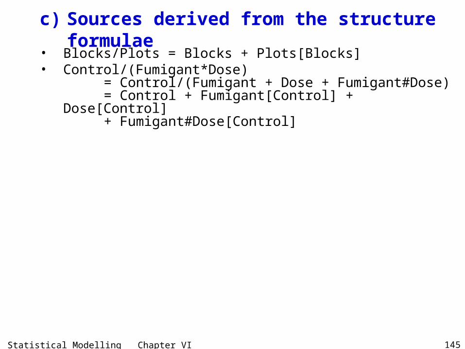
Statistical Modelling Chapter VI 145
c) Sources derived from the structure formulae• Blocks/Plots = Blocks + Plots[Blocks]• Control/(Fumigant*Dose)
= Control/(Fumigant + Dose + Fumigant#Dose)= Control + Fumigant[Control] + Dose[Control]
+ Fumigant#Dose[Control]

Statistical Modelling Chapter VI 146
d) Degrees of freedom and sums of squares

Statistical Modelling Chapter VI 147
e) The analysis of variance table
• Enter the sources for the study, their degrees of freedom and quadratic forms, into the ANOVA table below.
• Fixed factors: randomized factors• Random factors: unrandomized factors• The maximal variation and expectation models
are:– var[Y] = BlocksPlots + TreatmentsBlocks – = E[Y] = ControlDoseFumigant
f) Maximal expectation and variation models

Statistical Modelling Chapter VI 148
g) The expected mean squares
• The Hasse diagrams, with contributions to expected mean squares, for the unrandomized factors in this study are:
• Note that all the contributions of the randomized generalized factors will be of the form qF() as all the randomized factors are fixed.

Statistical Modelling Chapter VI 149
ANOVA table with E[MSq]
Source df SSq E[MSq]
Blocks 3 BY Q Y 2 2BP B12
Plots[Blocks] 44 BPY Q Y
Control 1 CY Q Y 2BP Cq
Dose[Control] 1 CDY Q Y 2BP CDq
Fumigant[Control] 3 CFY Q Y 2BP CFq
Dose#Fumigant[Control] 3 CDFY Q Y 2BP CDFq
Residual 36 ResBPY Q Y 2
BP
Total 47

Statistical Modelling Chapter VI 150
Example VI.19 A factorial experiment
• An experiment is to be conducted on sugar cane to investigate 6 factor (A, B, C, D, E, F) each at two levels.
• This experiment is to involve 16 blocks each of eight plots.
• The 64 treatment combinations are divided into 8 sets of 8 so that the ABCD, ABEF and ACE interactions are associated with set differences.
• The 8 sets are randomized to the 16 blocks so that each set occurs on two blocks and the 8 combinations in a set are randomized to the plots within a block.
• The sugar content of the cane is to be measured.

Statistical Modelling Chapter VI 151
a) Description of pertinent features of the study
1. Observational unit – a plot
2. Response variable– Sugar content
3. Unrandomized factors– Blocks, Plots
4. Randomized factors– A, B, C, D, E, F
5. Type of study– two replicates of a confounded 2k factorial
b) The experimental structure
Structure Formula unrandomized randomized

Statistical Modelling Chapter VI 152
c) Sources derived from the structure formulae
• How many main effects, two factor interactions, three-factor interactions and interactions of more than 3 factors are there?
– There are 6 main effects, 15 two-factor interactions, 20 three-factor interactions and 64 – 1 – 6 – 15 – 20 = 22 other interactions.
• What are the interactions confounded with blocks?
– The interactions confounded with blocks are ABCD, ABEF and ACE and all the products of these.
– That is ABCD, ABEF and ACE and CDEF, BDE, BCF, ADF

Statistical Modelling Chapter VI 153
d) Degrees of freedom and sums of squares• For the randomized sources, by the crossed structure
formula rule, all degrees of freedom will be 1 as all factors have 2 levels.

Statistical Modelling Chapter VI 154
e) The analysis of variance table
• Enter the sources for the study, their degrees of freedom and quadratic forms, into the ANOVA table below.
• Fixed factors:• Random factors:• The maximal variation and expectation models
are:– var[Y] =– = E[Y] =
f) Maximal expectation and variation models

Statistical Modelling Chapter VI 155
g) The expected mean squares • The Hasse diagrams, with contributions to expected
mean squares, for the unrandomized factors in this study are:
• Note that all the contributions of the randomized generalized factors will be of the form qF() as all the randomized factors are fixed.

Statistical Modelling Chapter VI 156
ANOVA table with E[MSq]Source df E[MSq]
Blocks 15
ACE 1 2 2BP B8 q ACE
ADF 1 2 2BP B8 q ADF
BCF 1 2 2BP B8 q BCF
BDE 1 2 2BP B8 q BDE
ABCD 1 2 2BP B8 q ABCD
ABEF 1 2 2BP B8 q ABEF
CDEF 1 2 2BP B8 q CDEF
Residual 8 2 2BP B8
Plots[Blocks] 112
main effects 6 2BP q i
2-factor interactions 15 2BP q i.j
3-factor interactions 17 2BP q i.j.k
other interactions 19 2BP q i.j.k.l+
Residual 55 2BP
• (just give the interactions confounded with blocks and the numbers of main effects, two-factor, three-factor and other interactions)