VHF/UHF/Microwave Radio Propagation: A Primer for DigitalExperimenters

Barry McLarnon, VE3JF2696 Regina St.

Ottawa, ON K2B 6Y1ve3jf@tapr.org

Abstract

This paper attempts to provide some insight into the nature of radio propagation in that part of thespectrum (upper VHF to microwave) used by experimenters for high-speed digital transmission. It beginswith the basics of free space path loss calculations, and then considers the effects of refraction, diffractionand reflections on the path loss of Line of Sight (LOS) links. The nature of non-LOS radio links is thenexamined, and propagation effects other than path loss which are important in digital transmission arealso described.

Introduction

The nature of packet radio is changing. As access to the Internet becomes cheaper and faster, and theapplications offered on the “net” more and more enticing, interest in the amateur packet radio networkwhich grew up in the 1980s steadily wanes. To be sure, there are still pockets of interest in some places,particularly where some infrastructure to support speeds of 9600 bps or more has been built up, but thishas not reversed the trend of declining interest and participation. Nevertheless, there is still lots ofinterest in packet radio out there - it is simply becoming re-focused in different areas. Some applicationswhich do not require high speed, and can take advantage of the mobility that packet radio can provide,have found a secure niche - APRS is a good example. Interest is also high in high-speed wirelesstransmission which can match, or preferably exceed, landline modem rates. With a wireless link, you canhave a 24-hour network connection without the need for a dedicated line, and you may also have thepossibility of portable or mobile operation. Until recently, most people have considered it to be just toodifficult to do high-speed digital. For example, the WA4DSY 56 Kbps RF modem has been available forten years now, and yet only a few hundred people at most have put one on the air. With the new versionof the modem introduced last year, 56 Kbps packet radio has edged closer to plug ‘n play, but in themeantime, landline modem data rates have moved into the same territory. What has really sparkedinterest in high-speed packet radio lately is not the amateur packet equipment, but the boom in spreadspectrum (SS) wireless LAN (WLAN) hardware which can be used without a licence in some of the ISMbands. The new WLAN units are typically integrated radio/modem/computer interfaces which mimiceither ethernet interfaces or landline modems, and are just as easy to set up. Many of them offer speedswhich landline modem users can only dream of. TAPR and others are working on bringing this type ofSS technology into the amateur service, where it can be used on different bands, and without theEffective Radiated Power (ERP) restrictions which exist for the unlicenced service. This technology willbe the ticket to developing high-speed wireless LANs and MANs which, using the Internet as abackbone, could finally realize the dream of a high-performance wide-area AMPRnet which can support

the applications (WWW, audio and video conferencing, etc.) that get people excited about computernetworking these days.

Although the dream as stated above is somewhat controversial, the author believes it represents the besthope of attracting new people to the hobby, providing a basis for experimentation and training in state-of-the-art wireless techniques and networking, and, ultimately, retaining spectrum for the amateur radioservice. One problem is that most of the people attracted to using digital wireless techniques have littleor no background in RF. When it comes to setting up wireless links which will work over some distance,they tend to lack the necessary knowledge about antennas, transmission lines and, especially, thesubtleties of radio propagation. This paper deals with the latter area, in the hopes of providing this newcrop of digital experimenters with some tools to help them build wireless links which work.

The main emphasis of this paper is on predicting the path loss of a link, so that one can approach theinstallation of the antennas and other RF equipment with some degree of confidence that the link willwork. The focus is on acquiring a feel for radio propagation, and pointing the way towards recognizingthe alternatives that may exist and the instances in which experimentation may be fruitful. We’ll also lookat some propagation aspects which are of particular relevance to digital signaling.

Estimating Path Loss

The fundamental aim of a radio link is to deliver sufficient signal power to the receiver at the far end ofthe link to achieve some performance objective. For a data transmission system, this objective is usuallyspecified as a minimum bit error rate (BER). In the receiver demodulator, the BER is a function of thesignal to noise ratio (SNR). At the frequencies under consideration here, the noise power is oftendominated by the internal receiver noise; however, this is not always the case, especially at the lower(VHF) end of the range. In addition, the “noise” may also include significant power from interferingsignals, necessitating the delivery of higher signal power to the receiver than would be the case undermore ideal circumstances (i.e., back-to-back through an attenuator). If the channel contains multipath,this may also have a major impact on the BER. We will consider multipath in more detail later - for now,we will focus on predicting the signal power which will be available to the receiver.

Free Space Propagation

The benchmark by which we measure the loss in a transmission link is the loss that would be expected infree space - in other words, the loss that would occur in a region which is free of all objects that mightabsorb or reflect radio energy. This represents the ideal case which we hope to approach in our realworld radio link (in fact, it is possible to have path loss which is less than the “free space” case, as weshall see later, but it is far more common to fall short of this goal).

Calculating free space transmission loss is quite simple. Consider a transmitter with power Pt coupled toan antenna which radiates equally in all directions (everyone’s favorite mythical antenna, the isotropicantenna). At a distance d from the transmitter, the radiated power is distributed uniformly over an area of4πd2 (i.e. the surface area of a sphere of radius d), so that the power flux density is:

sP

dt=

4 2π(1)

The transmission loss then depends on how much of this power is captured by the receiving antenna. Ifthe capture area, or effective aperture of this antenna is Ar, then the power which can be delivered to thereceiver (assuming no mismatch or feedline losses) is simply

P sAr r= (2)

For the hypothetical isotropic receiving antenna, we have

Ar =λπ

2

4(3)

Combining equations (1) and (3) into (2), we have

P Pdr t=

λπ4

2

(4)

The free space path loss between isotropic antennas is Pt / Pr. Since we usually are dealing withfrequency rather than wavelength, we can make the substitution λ = c/f to get

Lc

f dp =

42

2 2π(5)

This shows the classic square-law dependence of signal level versus distance. What troubles some peoplewhen they see this equation is that the path loss also increases as the square of the frequency. Does thismean that the transmission medium is inherently more lossy at higher frequencies? While it is true thatabsorption of RF by various materials (buildings, trees, water vapor, etc.) tends to increase withfrequency, remember we are talking about “free space” here. The frequency dependence in this case issolely due to the decreasing effective aperture of the receiving antenna as the frequency increases. This isintuitively reasonable, since the physical size of a given antenna type is inversely proportional tofrequency. If we double the frequency, the linear dimensions of the antenna decrease by a factor of one-half, and the capture area by a factor of one-quarter. The antenna therefore captures only one-quarter ofthe power flux density at the higher frequency versus the lower one, and delivers 6 dB less signal to thereceiver. However, in most cases we can easily get this 6 dB back by increasing the effective aperture,and hence the gain, of the receiving antenna. For example, suppose we are using a parabolic dish antennaat the lower frequency. When we double the frequency, instead of allowing the dish to be scaled down insize so as to produce the same gain as before, we can maintain the same reflector size. This gives us thesame effective aperture as before (assuming that the feed is properly redesigned for the new frequency,etc.), and 6 dB more gain (remembering that the gain is with respect to an isotropic or dipole referenceantenna at the same frequency). Thus the free space path loss is now the same at both frequencies;moreover, if we maintained the same physical aperture at both ends of the link, we would actually have 6dB less path loss at the higher frequency. You can picture this in terms of being able to focus the energymore tightly at the frequency with the shorter wavelength. It has the added benefit of providing greaterdiscrimination against multipath - more about this later.

The free space path loss equation is more usefully expressed logarithmically:

L f d dBp = + +32 4 20 20. log log (f in MHz, d in km) (6a)

or

L f d dBp = + +36 6 20 20. log log (f in MHz, d in miles) (6b)

This shows more clearly the relationship between path loss and distance: path loss increases by 20dB/decade or 6 dB/octave, so each time you double the distance, you lose another 6 dB of signal underfree space conditions.

Of course, in looking at a real system, we must consider the actual antenna gains and cable losses incalculating the signal power Pr which is available at the receiver input:

P P L G G L Lr t p t r t r= − + + − − (7)

where Pt = transmitter power output (dBm or dBW, same units as Pr)Lp = free space path loss between isotropic antennas (dB)Gt = transmit antenna gain (dBi)Gr = receive antenna gain (dBi)Lt = transmission line loss between transmitter and transmit antenna (dB)Lr = transmission line loss between receive antenna and receiver input (dB)

A table of transmission line losses for various bands and popular cable types can be found in theAppendix.

Example 1. Suppose you have a pair of 915 MHz WaveLAN cards, and want to use them on a 10 kmlink on which you believe free space path loss conditions will apply. The transmitter power is 0.25 W, or+24 dBm. You also have a pair of yagi antennas with 10 dBi gain, and at each end of the link, you needabout 50 ft (15 m) of transmission line to the antenna. Let’s say you’re using LMR-400 coaxial cable,which will give you about 2 dB loss at 915 MHz for each run. Finally, the path loss from equation (6a) iscalculated, and this gives 111.6 dB, which we’ll round off to 112 dB. The expected signal power at thereceiver is then, from (7):

P dBmr = − + + − − = −24 112 10 10 2 2 72

According to the WaveLAN specifications, the receivers require -78 dBm signal level in order to deliver alow bit error rate (BER). So, we should be in good shape, as we have 6 dB of margin over the minimumrequirement. However, this will only be true if the path really is equivalent to the free space case, andthis is a big if! We’ll look at means of predicting whether the free space assumption holds in the nextsection.

Path Loss on Line of Sight Links

The term Line of Sight (LOS) as applied to radio links has a pretty obvious meaning: the antennas at theends of the link can “see” each other, at least in a radio sense. In many cases, radio LOS equates tooptical LOS: you’re at the location of the antenna at one end of the link, and with the unaided eye orbinoculars, you can see the antenna (or its future site) at the other end of the link. In other cases, we maystill have an LOS path even though we can’t see the other end visually. This is because the radio horizonextends beyond the optical horizon. Radio waves follow slightly curved paths in the atmosphere, but ifthere is a direct path between the antennas which doesn’t pass through any obstacles, then we still haveradio LOS. Does having LOS mean that the path loss will be equal to the free space case which we havejust considered? In some cases, the answer is yes, but it is definitely not a sure thing. There are threemechanisms which may cause the path loss to differ from the free space case:

• refraction in the earth’s atmosphere, which alters the trajectory of radio waves, and which can changewith time.

• diffraction effects resulting from objects near the direct path. • reflections from objects, which may be either near or far from the direct path.

We examine these mechanisms in the next three sections.

Atmospheric Refraction

As mentioned previously, radio waves near the earth’s surface do not usually propagate in preciselystraight lines, but follow slightly curved paths. The reason is well-known to VHF/UHF DXers: refractionin the earth’s atmosphere. Under normal circumstances, the index of refraction decreases monotonicallywith increasing height, which causes the radio waves emanating from the transmitter to bend slightlydownwards towards the earth’s surface instead of following a straight line. The effect is morepronounced at radio frequencies than at the wavelength of visible light, and the result is that the radiowaves can propagate beyond the optical horizon, with no additional loss other than the free spacedistance loss. There is a convenient artifice which is used to account for this phenomenon: when the pathprofile is plotted, we reduce the curvature of the earth’s surface. If we choose the curvature properly, thepaths of the radio waves can be plotted as straight lines. Under normal conditions, the gradient inrefractivity index is such that real world propagation is equivalent to straight-line propagation over anearth whose radius is greater than the real one by a factor of 4/3 - thus the often-heard term “4/3 earthradius” in discussions of terrestrial propagation. However, this is just an approximation that appliesunder typical conditions - as VHF/UHF experimenters well know, unusual weather conditions can changethe refractivity profile dramatically. This can lead to several different conditions. In superrefraction, therays bend more than normal and the radio horizon is extended; in extreme cases, it leads to thephenomenon known as ducting, where the signal can propagate over enormous distances beyond thenormal horizon. This is exciting for DXers, but of little practical use for people who want to run datalinks. The main consequence for digital experimenters is that they may occasionally experienceinterference from unexpected sources. A more serious concern is subrefraction, in which the bending ofthe rays is less than normal, thus shortening the radio horizon and reducing the clearance over obstaclesalong the path. This may lead to increased path loss, and possibly even an outage. In commercial radiolink planning, the statistical probability of these events is calculated and allowed for in the link design

(distance, path clearance, fading margin, etc.). We won’t get into all of the details here; suffice it to saythat reliability of your link will tend to be higher if you back off the distance from the maximum which isdictated by the normal radio horizon. Not that you shouldn’t try and stretch the limits when the needarises, but a link which has optical clearance is preferable to one which doesn’t. It’s also a good idea tobuild in some margin to allow for fading due to unusual propagation situations, and to allow as muchclearance from obstacles along the path as possible. For short-range links, the effects of refraction canusually be ignored.

Diffraction and Fresnel Zones

Refraction and reflection of radio waves are mechanisms which are fairly easy to picture, but diffraction ismuch less intuitive. To understand diffraction, and radio propagation in general, it is very helpful to havesome feeling for how radio waves behave in an environment which is not strictly “free space”. ConsiderFig. 1, in which a wavefront is traveling from left to right, and encountering an obstacle which absorbs orreflects all of the incident radio energy. Assume that the incident wavefront is uniform; i.e., if wemeasure the field strength along the line A-A’, it is the same at all points. Now, what will be the fieldstrength along a line B-B’ on the other side of the obstacle? To quantify this, we provide an axis in whichzero coincides with the top of the obstacle, and negative and positive numbers denote positions aboveand below this, respectively (we’ll define the parameter ν used on this axis a bit later).

Figure 1 Shadowing of Radio Waves by an Object

Intuition may lead one to expect the field strength along B-B’ to look like the dashed line in Fig. 2, withcomplete shadowing and zero signal below the top of the obstacle, and no effect at all above it. The solidline shows the reality: not only does energy “leak” into the shadowed area, but the field strength abovethe top of the obstacle is also disturbed. At a position which is level with the top of the obstacle, thesignal power density is down by some 6 dB, despite the fact that this point is in “line of sight” of thesource. This effect is less surprising when one considers other familiar instances of wave motion.Picture, for example, tossing a rock in a pond and watching the ripples propagate outward. When theyencounter an object such as a boat or a pier, you will see that the water behind the object is alsodisturbed, and that the waves traveling past, but close to, the object are also affected somewhat.Similarly, consider a distant source of sound waves: if the sound level is well above the ambient level,then moving behind an object which absorbs the incident sound energy completely does not result in thesound disappearing completely - it is still audible at a lower level, due to diffraction (as an aside, it isinteresting to note that the wavelength of a 1 KHz sound wave is nearly the same as a 1 GHz radiowave). So much for analogies - let’s get back to radio waves.

The explanation for the non-intuitive behavior of radio waves in the presence of obstacles which appear intheir path is found in something called Huygens’ Principle. Huygens showed that propagation occurs asfollows: each point on a wavefront acts as a source of a secondary wavefront known as a wavelet, and anew wavefront is then built up from the combination of the contributions from all of the wavelets on thepreceding wavefront. The secondary wavelets do not radiate equally in all directions - their amplitude in

Figure 2 Signal Levels on the Far Side of the Shadowing Object

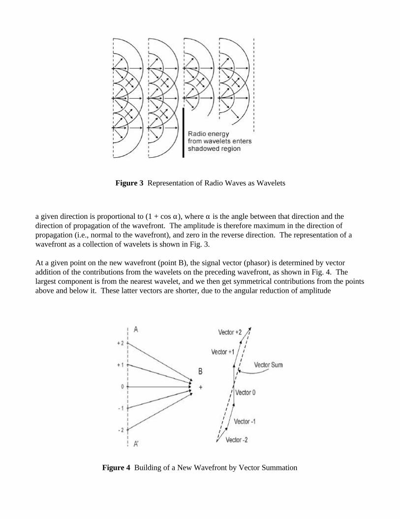
a given direction is proportional to (1 + cos α), where α is the angle between that direction and thedirection of propagation of the wavefront. The amplitude is therefore maximum in the direction ofpropagation (i.e., normal to the wavefront), and zero in the reverse direction. The representation of awavefront as a collection of wavelets is shown in Fig. 3.

At a given point on the new wavefront (point B), the signal vector (phasor) is determined by vectoraddition of the contributions from the wavelets on the preceding wavefront, as shown in Fig. 4. Thelargest component is from the nearest wavelet, and we then get symmetrical contributions from the pointsabove and below it. These latter vectors are shorter, due to the angular reduction of amplitude

Figure 3 Representation of Radio Waves as Wavelets

Figure 4 Building of a New Wavefront by Vector Summation

mentioned above, and also the greater distance traveled. The greater distance also introduces more timedelay, and hence the rotation of the vectors as shown in the figure. As we include contributions frompoints farther and farther away, the corresponding vectors continue to rotate and diminish in length, andthey trace out a double-sided spiral path, known as the Cornu spiral.

The Cornu spiral, shown in Fig. 5, provides the tool we need to visualize what happens when radio wavesencounter an obstacle. In free space, at every point on a new wavefront, all contributions from thewavelets on the preceding wavefront are present and unattenuated, so the resultant vector corresponds tothe complete spiral (i.e., the endpoints of the vector are X and Y). Now, consider again the situationshown in Fig. 1, and for each location on the wavefront B-B’, visualize the makeup of the Cornu spiral(note that the top of the obstacle is assumed to be sufficiently narrow that no significant reflections canoccur from it). At position 0, level with the top of the obstacle, we will have only contributions from thepositive half of the preceding wavefront at A-A’, since all of the others are blocked by the obstacle.Therefore, the received components form only the upper half of the spiral, and the resultant vector isexactly half the length of the free space case, corresponding to a 6 dB reduction in amplitude. As we golower on the line B-B’, we start to get blockage of components from the positive side of the A-A’wavefront, removing more and more of the vectors as we go, and leaving only the tight upper spiral. Theresulting amplitude diminishes monotonically towards zero as we move down the new wavefront, butthere is still signal present at all points behind the obstacle, as shown in the graph in Fig. 2. How aboutthe points along line B-B’ above the obstacle, where the graph shows those mysterious ripples? Again,look at the Cornu spiral: as we move up the line, we begin to add contributions from the negative side ofthe A-A’ wavefront (vectors -1, -2, etc.). Note what happens to the resultant vector - as we make thefirst turn around the bottom of the spiral, it reaches its maximum length, corresponding to the highest

Figure 5 The Cornu Spiral

peak in the graph of Fig. 2. As we continue to move up B-B’ and add more components, we swingaround the spiral and reach the minimum length for the resultant vector (minimum distance from pointY). Further progression up B-B’ results in further motion around the spiral, and the amplitude of theresultant oscillates back and forth, with the amplitude of the oscillation steadily decreasing as theresultant converges on the free space value, given by the complete Cornu spiral (vector X-Y).

So, in a nutshell, to visualize what happens to radio waves when they encounter an obstacle, we have todevelop a picture of the wavefront after the obstacle as a function of the wavefront just before it (asopposed to simply tracing rays from the distant source). Now we’re in a position to talk about Fresnelzones. A Fresnel zone is a simpler concept once you have some understanding of diffraction: it is thevolume of space enclosed by an ellipsoid which has the two antennas at the ends of a radio link at its foci.The two-dimensional representation of a Fresnel zone is shown in Fig. 6. The surface of the ellipsoid isdefined by the path ACB, which exceeds the length of the direct path AB by some fixed amount. Thisamount is nλ/2, where n is a positive integer. For the first Fresnel zone, n = 1 and the path length differsby λ/2 (i.e., a 180° phase reversal with respect to the direct path). For most practical purposes, only thefirst Fresnel zone need be considered. A radio path has first Fresnel zone clearance if, as shown in Fig.6, no objects capable of causing significant diffraction penetrate the corresponding ellipsoid. What doesthis mean in terms of path loss? Recall how we constructed the wavefront behind an object by vectoraddition of the wavelets comprising the wavefront in front of the object, and apply this to the case wherewe have exactly first Fresnel zone clearance. We wish to find the strength of the direct path signal after itpasses the object. Assuming there is only one such object near the Fresnel zone, we can look at theresultant wavefront at the destination point B. In terms of the Cornu spiral, the upper half of the spiral isintact, but part of the lower half is absent, due to blockage by the object. Since we have exactly firstFresnel clearance, the final vector which we add to the bottom of the spiral is 180° out of phase with thedirect-path vector - i.e., it is pointing downwards. This means that we have passed the bottom of thespiral and are on the way back up, and the resultant vector is near the free space magnitude (a linebetween X and Y in Fig. 5). In fact, it is sufficient to have 60% of the first Fresnel clearance, since thiswill still give a resultant which is very close to the free space value.

In order to quantify diffraction losses, they are usually expressed in terms of a dimensionless parameter ν,given by:

vd

= 2∆λ

(8)

Figure 6 Fresnel Zone for a Radio Link

where ∆d is the difference in lengths of the straight-line path between the endpoints of the link and thepath which just touches the tip of the diffracting object (see Fig. 7, where ∆d = d1 + d2 - d). Byconvention, ν is positive when the direct path is blocked (i.e., the obstacle has positive height), andnegative when the direct path has some clearance (“negative height”). When the direct path just grazesthe object, ν = 0. This is the parameter shown in Figures 1 and 2. Since in this section we areconsidering LOS paths, this corresponds to specifying that ν ó 0. For first Fresnel zone clearance, wehave ∆d = λ/2, so from equation (8), ν = -1.4. From Fig. 2, we can see that this is more clearance thannecessary - in fact, we get slightly higher signal level (and path loss less than the free space value) if wereduce the clearance to ν = -1, which corresponds to ∆d = λ/4. The ν = -1 point is also shown on theCornu spiral in Fig. 5. Since ∆d= λ/4, the last vector added to the summation is rotated 90° from thedirect-path vector, which brings us to the lowest point on the spiral. The resultant vector then runs fromthis point to the upper end of the spiral at point Y. It’s easy to see that this vector is a bit longer than thedistance from X to Y, so we have a slight gain (about 1.2 dB) over the free space case. We can also seehow we can back off to 60% of first Fresnel zone clearance (ν ≈ -0.85) without suffering significant loss.

But how do we calculate whether we have the required clearance? The geometry for Fresnel zonecalculations is shown in Fig. 7. Keep in mind that this is only a two-dimensional representation, butFresnel zones are three-dimensional. The same considerations apply when the objects limiting pathclearance are to the side or even above the radio path. Since we are considering LOS paths in thissection, we are dealing only with the “negative height” case, shown in the lower part of the figure. Wewill look at the case where h is positive later, when we consider non-LOS paths.

For first Fresnel zone clearance, the distance h from the nearest point of the obstacle to the direct pathmust be at least

hd d

d d=

+2 1 2

1 2

λ(9)

where d1 and d2 are the distances from the tip of the obstacle to the two ends of the radio circuit. Thisformula is an approximation which is not valid very close to the endpoints of the circuit. Forconvenience, the clearance can be expressed in terms of frequency:

hd d

f d d=

+17 3 1 2

1 2

.( )

(10a)

where f is the frequency in GHz, d1 and d2 are in km, and h is in meters. Or:

hd d

f d d=

+721 1 2

1 2

.( )

(10b)

where f is in GHz, d1 and d2 in statute miles, and h is in feet.

Example 2. We have a 10 km LOS path over which we wish to establish a link in the 915 MHz band.The path profile indicates that the high point on the path is 3 km from one end, and the direct path clearsit by about 18 meters (60 ft.) - do we have adequate Fresnel zone clearance? From equation (10a), withd1 = 3 km, d2 = 7 km, and f = 0.915 GHz, we have h = 26.2 m for first Fresnel zone clearance (strictlyspeaking, h = -26.2 m). A clearance of 18 m is about 70% of this, so it is sufficient to allow negligiblediffraction loss.

Fresnel zone clearance may not seem all that important - after all, we said previously that for the zeroclearance (grazing) case, we have 6 dB of additional path loss. If necessary, this could be overcome with,for example, an additional 3 dB of antenna gain at each end of the circuit. Now it’s time to confess thatthe situation depicted in Figures 1 and 2 is a special case, known as “knife edge” diffraction. Basically,this means that the top of the obstacle is small in terms of wavelengths. This is sometimes a reasonableapproximation of an object in the real world, but more often than not, the obstacle will be rounded (suchas a hilltop) or have a large flat surface (like the top of a building), or otherwise depart from the knifeedge assumption. In such cases, the path loss for the grazing case can be considerably more than 6 dB -in fact, 20 dB would be a better estimate in many cases. So, Fresnel zone clearance can be prettyimportant on real-world paths. And, again, keep in mind that the Fresnel zone is three-dimensional, soclearance must also be maintained from the sides of buildings, etc. if path loss is to be minimized.Another point to consider is the effect on Fresnel zone clearance of changes in atmospheric refraction, asdiscussed in the last section. We may have adequate clearance on a longer path under normal conditions(i.e., 4/3 earth radius), but lose the clearance when unusual refraction conditions prevail. On longerpaths, therefore, it is common in commercial radio links to do the Fresnel zone analysis on something

Figure 7 Fresnel Zone Geometry

close to “worst case” rather than typical refraction conditions, but this may be less of a concern inamateur applications.

Most of the material in this section was based on Ref. [2], which is highly recommended for furtherreading.

Ground Reflections

An LOS path may have adequate Fresnel zone clearance, and yet still have a path loss which differssignificantly from free space under normal refraction conditions. If this is the case, the cause is probablymultipath propagation resulting from reflections (multipath also poses particular problems for digitaltransmission systems - we’ll look at this a bit later, but here we are only considering path loss).

One common source of reflections is the ground. It tends to be more of a factor on paths in rural areas;in urban settings, the ground reflection path will often be blocked by the clutter of buildings, trees, etc. Inpaths over relatively smooth ground or bodies of water, however, ground reflections can be a majordeterminant of path loss. For any radio link, it is worthwhile to look at the path profile and see if theground reflection has the potential to be significant. It should also be kept in mind that the reflectionpoint is not at the midpoint of the path unless the antennas are at the same height and the ground is notsloped in the reflection region - just the remember the old maxim from optics that the angle of incidenceequals the angle of reflection.

Ground reflections can be good news or bad news, but are more often the latter. In a radio pathconsisting of a direct path plus a ground-reflected path, the path loss depends on the relative amplitudeand phase relationship of the signals propagated by the two paths. In extreme cases, where the ground-reflected path has Fresnel clearance and suffers little loss from the reflection itself (or attenuation fromtrees, etc.), then its amplitude may approach that of the direct path. Then, depending on the relativephase shift of the two paths, we may have an enhancement of up to 6 dB over the direct path alone, orcancellation resulting in additional path loss of 20 dB or more. If you are acquainted with Mr. Murphy,you know which to expect! The difference in path lengths can be estimated from the path profile, andthen translated into wavelengths to give the phase relationship. Then we have to account for thereflection itself, and this is where things get interesting. The amplitude and phase of the reflected wavedepend on a number of variables, including conductivity and permittivity of the reflecting surface,frequency, angle of incidence, and polarization.

It is difficult to summarize the effects of all of the variables which affect ground reflections, but a typicalcase is shown in Fig. 8 [2]. This particular figure is for typical ground conditions at 100 MHz, but thesame behavior is seen over a wide range of ground constants and frequencies. Notice that there is a largedifference in reflection amplitudes between horizontal and vertical polarization (denoted on the curveswith “h” and “v”, respectively), and that vertical polarization in general gives rise to a much smallerreflected wave. However, the difference is large only for angles of incidence greater than a few degrees(note that, unlike in optics, in radio transmission the angle of incidence is normally measured with respectto a tangent to the reflecting surface rather than a normal to it); in practice, these angles will only occuron very short paths, or paths with extraordinarily high antennas. For typical paths, the angle of incidencetends to be of the order of one degree or less - for example, for a 10 km path over smooth earth with 10m antenna heights, the angle of incidence of the ground reflection would only be about 0.11 degrees. Insuch a case, both polarizations will give reflection amplitudes near unity (i.e., no reflection loss). Perhaps

more surprisingly, there will also be a phase reversal in both cases. Horizontally-polarized waves alwaysundergo a phase reversal upon reflection, but for vertically-polarized waves, the phase change is afunction of the angle of incidence and the ground characteristics.

The upshot of all this is that for most paths in which the ground reflection is significant (and no otherreflections are present), there will be very little difference in performance between horizontal and verticalpolarization. For very short paths, horizontal polarization will generally give rise to a stronger reflection.If it turns out that this causes cancellation rather than enhancement, switching to vertical polarization mayprovide a solution. In other words, for shorter paths, it is usually worthwhile to try both polarizations tosee which works better (of course, other factors such as mounting constraints and rejection of othersources of multipath and interference also enter into the choice of polarization).

As stated above, for either polarization, as the path gets longer we approach the case where the groundreflection produces a phase reversal and very little attenuation. At the same time, the direct and reflectedpaths are becoming more nearly equal. The path loss ripples up and down as we increase the distance,until we reach the point where the path lengths differ by just one-half wavelength. Combined with the180° phase shift caused by the ground reflection, this brings the direct and reflected signals into phase,resulting in an enhancement over the free space path loss (theoretically 6 dB, but this will seldom berealized in practice). Thereafter, it’s all downhill as the distance is further increased, since phasedifference between the two paths approaches in the limit the 180° phase shift of the ground reflection. Itcan be shown that, in this region, the received power follows an inverse fourth-power law as a function of

Figure 8 Typical Ground Reflection Parameters

distance instead of the usual square law (i.e., 12 dB more attenuation when you double the distance,instead of 6 dB). The distance at which the path loss starts to increase at the fourth-power rate isreached when the ellipsoid corresponding to the first Fresnel zone just touches the ground. A reasonablygoodestimate of this distance can be calculated from the equation

dh h

=4 1 2

λ(11)

where h1 and h2 are the antenna heights above the ground reflection point. For example, for antennaheights of 10 m, at 915 MHz (λ = 33 cm) we will be into the fourth-law loss region for links longer thanabout 1.2 km.

So, for longer-range paths, ground reflections are always bad news. Serious problems with groundreflections are most commonly encountered with radio links across bodies of water. Spread spectrumtechniques and diversity antenna arrangements usually can’t overcome the problems - the solution lies insiting the antennas (e.g., away from the shore of the body of water) such that the reflected path is cut offby natural obstacles, while the direct path is unimpaired. In other cases, it may be possible to adjust theantenna locations so as to move the reflection point to a rough area of land which scatters the signalrather than creating a strong specular reflection.

Other Sources of Reflections

Much of what has been said about ground reflections applies to reflections from other objects as well.The “ground reflection” on a particular path may be from a building rooftop rather than the ground itself,but the effect is much the same. On long links, reflections from objects near the line of the direct pathwill almost always cause increased path loss - in essence, you have a permanent “flat fade” over a verywide bandwidth. Reflections from objects which are well off to the side of the direct path are a differentstory, however. This is a frequent occurrence in urban areas, where the sides of buildings can causestrong reflections. In such cases, the angle of incidence may be much larger than zero, unlike the groundreflection case. This means that horizontal and vertical polarization may behave quite differently - as wesaw in Fig. 8, vertically polarized signals tend to produce lower-amplitude reflections than horizontallypolarized signals when the angle of incidence exceeds a few degrees. When the reflecting surface isvertical, like the side of a building, a signal which is transmitted with horizontal polarization effectivelyhas vertical polarization as far as the reflection is concerned. Therefore, horizontal polarization willgenerally result in weaker reflections and less multipath than vertical polarization in these cases.

Effects of Rain, Snow and Fog

The loss of LOS paths may sometimes be affected by weather conditions (other than the refraction effectswhich have already been mentioned). Rain and fog (clouds) become a significant source of attenuationonly when we get well into the microwave region. Attenuation from fog only becomes noticeable (i.e.,attenuation of the order of 1 dB or more) above about 30 GHz. Snow is in this category as well. Rainattenuation becomes significant at around 10 GHz, where a heavy rainfall may cause additional path lossof the order of 1 dB/km.

Path Loss on Non-Line of Sight Paths

We have spent quite a bit of time looking at LOS paths, and described the mechanisms which often causethem to have path loss which differs from the “free space” assumption. We’ve seen that the path lossisn’t always easy to predict. When we have a path which is not LOS, it becomes even more difficult topredict how well signals will propagate over it. Unfortunately, non-LOS situations are sometimesunavoidable, particularly in urban areas. The following sections deal with some of the major factorswhich must be considered.

Diffraction Losses

In some special cases, such as diffraction over a single obstacle which can be modeled as a knife edge, theloss of a non-LOS path can be predicted fairly readily. In fact, this is the same situation that we saw inFigures 1 and 2, with the diffraction parameter ν > 0. This parameter, from equation (8), is

vd

= 2∆λ

To get ∆d, measure the straight-line distance between the endpoints of the link. Then measure the lengthof the actual path, which includes the two endpoints and the tip of the knife edge, and take the differencebetween the two. The geometry is shown in Fig. 7(a), the “positive h” case. A good approximation tothe knife-edge diffraction loss in dB can then be calculated from

( ) [ ]L v v v= + + +69 20 12. log (12)

Example 3. We want to run a 915 MHz link between two points which are a straight-line distance of 25km apart. However, 5 km from one end of the link, there is a ridge which is 100 meters higher than thetwo endpoints. Assuming that the ridge can be modeled as a knife edge, and that the paths from theendpoints to the top of ridge are LOS with adequate Fresnel zone clearance, what is the expected pathloss? From simple geometry, we find that length of the path over the ridge is 25,001.25 meters, so that∆d = 1.25 m. Since λ = 0.33 m, the parameter ν, from (8), is 3.89. Substituting this into (12), we findthat the expected diffraction loss is 24.9 dB. The free space path loss for a 25 km path at 915 MHz is,from equation (6a), 119.6 dB, so the total predicted path loss for this path is 144.5 dB. This is too lossya path for many WLAN devices. For example, suppose we are using WaveLAN cards with 13 dBi gainantennas, which (disregarding feedline losses) brings them up to the maximum allowable EIRP of +36dBm. This will produce, at the antenna terminals at the other end of the link, a received power of (36 -144.5 + 13) = -95.5 dBm. This falls well short of the -78 dBm requirement of the WaveLAN cards. Onthe other hand, a lower-speed system may be quite usable over this path. For instance, the FreeWave 115Kbps modems require only about -108 dBm for reliable operation, which is a comfortable margin belowour predicted signal levels.

To see the effect of operating frequency on diffraction losses, we can repeat the calculation, this timeusing 144 MHz, and find the predicted diffraction loss to be 17.5 dB, or 7.4 dB less than at 915 MHz. At2.4 GHz, the predicted loss is 29.0 dB, an increase of 4.1 dB over the 915 MHz case (these differencesare for the diffraction losses only, not the only total path loss).

Unfortunately, the paths which digital experimenters are faced with are seldom this simple. They willfrequently involve diffraction over multiple rooftops or other obstacles, many of which don’t resembleknife edges. The path losses will generally be substantially greater in these cases than predicted by thesingle knife edge model. The paths will also often pass through objects such as trees and wood-framebuildings which are semi-transparent at radio frequencies. Many models have been developed to try andpredict path losses in these more complex cases. The most successful are those which deal with restrictedscenarios rather than trying to cover all of the possibilities. One common scenario is diffraction over asingle obstacle which is too rounded to be considered a knife edge. There are different ways of treatingthis problem; the one described here is from Ref. [3]. The top of the object is modeled as a cylinder ofradius r, as shown in Fig. 9. To calculate the loss, you need to plot the profile of the actual object, andthen draw straight lines from the link endpoints such that they just graze the highest part of the object asseen from their individual perspectives. Then the parameters Ds, d1, d2 and α are estimated, and anestimate of the radius r can then be calculated from

rD d d

d ds=+

2 1 2

12

22α ( )

(13)

Note that the angle α is measured in radians. The procedure then is to calculate the knife edge diffractionloss for this path as outlined above, and then add to it an excess loss factor Lex, calculated from

Lr

dBex = 117. απλ

(14)

Figure 9 Diffraction by a Rounded Obstacle

There is also a correction factor for roughness: if the object is, for example, a hill which is tree-coveredrather than smooth at the top, the excess diffraction loss is said to be about 65% of that predicted in (14).In general, smoother objects produce greater diffraction losses.

Example 4. We revisit the scenario in Example 3, but let’s suppose that we’ve now decided that theridge blocking our path doesn’t cut it as a knife edge (ouch!). From a plot of the profile, we estimate thatDs = 10 meters. As before, d1 = 20 km, d2 = 5 km and the height of the ridge is 100 meters. Dusting offour high school trigonometry, we can work out that α = 1.43°, or 0.025 radians. Now, plugging thesenumbers into (13), we get r = 188 meters. Then, with λ = 0.33 m, we can calculate the excess loss from(14):

L dBex = × ××

=117 0 025188

0 3312 4. .

..

π

So, summed with the knife edge loss calculated previously, we have an estimated total diffraction loss of37.3 dB (assuming the ridge is “smooth” rather than “rough”). This is a lot, but you can easily imaginescenarios where the losses are much greater: just look at the direct dependence on the angle α in (14) andpicture from Fig. 9 what happens when the obstacle is closer to one of the link endpoints. Amateursdoing weak signal work are accustomed to dealing with large path losses in non-LOS propagation, butsuch losses are usually intolerable in high-speed digital links.

Attenuation from Trees and Forests

Trees can be a significant source of path loss, and there are a number of variables involved, such as thespecific type of tree, whether it is wet or dry, and in the case of deciduous trees, whether the leaves arepresent or not. Isolated trees are not usually a major problem, but a dense forest is another story. Theattenuation depends on the distance the signal must penetrate through the forest, and it increases withfrequency. According to a CCIR report [10], the attenuation is of the order of 0.05 dB/m at 200 MHz,0.1 dB/m at 500 MHz, 0.2 dB/m at 1 GHz, 0.3 dB/m at 2 GHz and 0.4 dB/m at 3 GHz. At lowerfrequencies, the attenuation is somewhat lower for horizontal polarization than for vertical, but thedifference disappears above about 1 GHz. This adds up to a lot of excess path loss if your signal mustpenetrate several hundred meters of forest! Fortunately, there is also significant propagation bydiffraction over the treetops, especially if you can get your antennas up near treetop level or keep them agood distance from the edge of the forest, so all is not lost if you live near a forest.

General Non-LOS Propagation Models

There are many more general models and empirical techniques for predicting non-LOS path losses, butthe details are beyond the scope of this paper. Most of them are aimed at prediction of the pathsbetween elevated base stations and mobile or portable stations near ground level, and they typically haverestrictions on the frequency range and distances for which they are valid; thus they may be of limitedusefulness in the planning of amateur high-speed digital links. Nevertheless, they are well worth studyingto gain further insight into the nature of non-LOS propagation. The details are available in many texts -Ref. [3] has a particularly good treatment. One crude, but useful, approximation will be mentioned here:the loss on many non-LOS paths in urban areas can be modeled quite well by a fourth-power distancelaw. In other words, we substitute d4 for d2 in equation (5). In equation (6), we can substitute 40log(d)for the 20log(d) term, which would correspond to the assumption of square-law distance loss for

distances up to 1 km (or 1 mile, for the non-metric version of the equation), and fourth-law lossthereafter. This is probably an overly optimistic assumption for heavily built-up areas, but is at least auseful starting point.

The propagation losses on non-LOS paths can be discouragingly high, particularly in urban areas.Antenna height becomes a critical factor, and getting your antennas up above rooftop heights will oftenspell the difference between success and failure. Due to the great variability of propagation in clutteredurban environments, accurate path loss predictions can be difficult. If a preliminary analysis of the pathindicates that you are at least in the ballpark (say within 10 or 15 dB) of having a usable link, then it willgenerally be worthwhile to give it a try and hope to be pleasantly surprised (but be prepared to bedisappointed!).

Software Tools for Propagation Prediction

Although there is no substitute for experience and acquiring a “feel” for radio propagation, computerprograms can make the job of predicting radio link performance a lot easier. They are particularly handyfor exploring “what if” scenarios with different paths, antenna heights, etc. Unfortunately, they also tendto cost money! If you’re lucky, you may have access to one of the sophisticated prediction programswhich includes the most complex propagation models, terrain databases, etc. If not, you can still findsome free software utilities that will make it easier to do some of the calculations discussed above, suchas knife edge diffraction losses. One very useful freeware program which was developed specifically forshort-range VHF/UHF applications is RFProp, by Colin Seymour, G4NNA. Check Colin’s Web page athttp://www.users.dircon.co.uk/~netking/freesw.htm for more information and downloading instructions.This is a Windows (3.1, 95 or NT) program which can calculate path loss in free space and simplediffraction scenarios. In addition to calculating knife edge diffraction loss, it provides some correctionfactors for estimating the loss caused by more rounded objects, such as hills. It also allows changing thedistance loss exponent from square-law to fourth-law (or anything else, for that matter) to simulate longpaths with ground reflections or obstructed urban paths. There is also some provision for estimating theloss caused when the signals must penetrate buildings. The program has a graphical user interface inwhich the major path parameters can be entered and the result (in terms of receiver SNR margin) seenimmediately. There is also a tabular output which lists the detailed results along with all of the assumedparameters.

Special Considerations for Digital Systems

We have previously looked at the effect of multipath on path loss. When reflections occur from objectswhich are very close to the direct path, then paths have very similar lengths and nearly the same timedelay. Depending on the relative phase shifts of the paths, the signals traversing them at a givenfrequency can add constructively to provide a gain with respect to a single path, or destructively toprovide a loss. On longer paths in particular, the effect is usually a loss. Since the path lengths are nearlyequal, the loss occurs over a wide frequency range, producing a “flat” fade.

In many cases, however, reflections from objects well away from the direct path can give rise tosignificant multipath. The most common reflectors are buildings and other manmade structures, but manynatural features can also be good reflectors. In such cases, the propagation delays of the paths from oneend of the link to the other can differ considerably. The extent of this time spreading of the signal is

commonly measured by a parameter known as the delay spread of the path. One consequence of havinga larger delay spread is that the reinforcement and cancellation effects will now vary more rapidly withfrequency. For example, suppose we have two paths with equal attenuation and which differ in length by300 meters, corresponding to a delay difference of 1 µsec. In the frequency domain, this link will havedeep nulls at intervals of 1 MHz, with maxima in between. With a narrowband system, you may be luckyand be operating at a frequency near a maximum, or you may be unlucky and be near a null, in which caseyou lose most of your signal (techniques such as space diversity reception may help, though). The pathloss in this case is highly frequency-dependent. On the other hand, a wideband signal which is, say,several MHz wide, would be subject to only partial cancellation or selective fading. Depending on thenature of the signal and how information is encoded into it, it may be quite tolerant of having part of itsenergy notched out by the multipath channel. Tolerance of multipath-induced signal cancellation is oneof the major benefits of spread spectrum transmission techniques.

Longer multipath delay spreads have another consequence where digital signals are concerned, however:overlap of received data symbols with adjacent symbols, known as intersymbol interference or ISI.Suppose we try to transmit a 1 Mbps data stream over the two-path multipath channel mentioned above.Assuming a modulation scheme with 1 µsec symbol length is used, then the signals arriving over the twopaths will be offset by exactly one symbol period. Each received symbol arriving over the shorter pathwill be overlaid by a copy of the previous symbol from the longer path, making it impossible to decodewith standard demodulation techniques. This problem can be solved by using an adaptive equalizer in thereceiver, but this level of sophistication is not commonly found in amateur or WLAN modems (but it willcertainly become more common as speeds continue to increase). Another way to attack this problem isto increase the symbol length while maintaining a high bit rate by using a multicarrier modulation schemesuch as OFDM (Orthogonal Frequency Division Multiplex), but again, such techniques are seldom foundin the wireless modem equipment available to hobbyists. For unequalized multipath channels, the delayspread must be much less than the symbol length, or the link performance will suffer greatly. The effectof multipath-induced ISI is to establish an irreducible error rate - beyond a certain point, increasingtransmitter power will cause no improvement in BER, since the BER vs Eb/N0 curve has gone flat. Acommon rule of thumb prescribes that the multipath delay spread should be no more than about 10% ofthe symbol length. This will generally keep the irreducible error rate down to the order of 10-3 or less.Thus, in our two-path example above, a system running at 100K symbols/s or less may worksatisfactorily. The actual raw BER requirements for a particular system will of course depend on theerror-control coding technique used.

Delay spreads of several microseconds are not uncommon, especially in urban areas. Mountainous areascan produce much longer delay spreads, sometimes tens of microseconds. This spells big trouble fordoing high-speed data transmission in these areas. The best way to mitigate multipath in these situationsis to use highly directional antennas, preferably at both ends of the link. The higher the data rate, themore critical it becomes to use high-gain antennas. This is one advantage to going higher in frequency.The delay spread for a given link will usually not exhibit much frequency dependence - for example, therewill be similar amounts of multipath whether you operate at 450 MHz or 2.4 GHz, if you use the sameantenna gain and type. However, you can get more directivity at the higher frequencies, which often willresult in significantly reduced multipath delay spread and hence lower BER. It may seem strange thathigh-speed WLAN products are often supplied with omnidirectional antennas which do nothing tocombat multipath, but this is because the antennas are intended for indoor use. The attenuation providedby the building structure will usually cause a drastic reduction in the amplitude of reflections from outside

the building, as well as from distant areas inside the building. Delay spreads therefore tend to be muchsmaller inside buildings - typically of the order of 0.1 µsec or less. However, as WLAN products withdata rates of 10 Mbps and beyond are now appearing, even delay spreads of this magnitude areproblematic and must be dealt with by such measures as equalizers, high-level modulation schemes andsectorized antennas.

Conclusions

Radio propagation is a vast topic, and we’ve only scratched the surface here. We haven’t considered, forexample, the interesting area of data transmission involving mobile stations - maybe next year! Hopefully,this paper has provided some insight into the problems and solutions associated with setting up digitallinks in the VHF to microwave spectrum. To sum up, here are a few guidelines and principles:

• Always strive for LOS conditions. Even with LOS, you must pay attention to details regardingvariability of refractivity, Fresnel zone clearance and avoiding reflections from the ground and othersurfaces. Non-LOS paths will often lead to disappointment unless they are very short, especially withthe high-speed unlicenced WLAN devices. Their low ERP limits and high receive signal powerrequirements (due to large noise bandwidths, high noise figures and sometimes, significant modemimplementation losses) leave little margin for higher-than-LOS path losses. Hams are notencumbered by the low ERP limits, but it can be very expensive to overcome excessive path losseswith higher transmitter powers.

• Use as much antenna gain as is practical. It is always worthwhile to try both polarizations, but

horizontal polarization will often be superior to vertical. It will generally provide less multipath inurban areas, and may provide lower path loss in some non-LOS situations (e.g., attenuation fromtrees at VHF and lower UHF). Also, interfering signals from pagers and the like tend to be verticallypolarized, so using the opposite polarization can often provide some protection from them.

• There are advantages to going higher in frequency, into the microwave bands, due to the higher

antenna gains which can be achieved. The tighter focusing of energy which can be achieved mayresult in lower overall path loss on LOS paths (providing that you can keep the feedline losses undercontrol), and less multipath. Higher frequencies also have smaller Fresnel zones, and thus require lessclearance over obstacles to avoid diffraction losses. And, of course, the higher bands have morebandwidth available for high-speed data, and less probability of interference. However, the advantagemay be lost in non-LOS situations, since diffraction losses, and attenuation from natural objects suchas trees, increase with frequency.

Radio propagation is seldom 100% predictable, and one should never hesitate to experiment. It’s veryuseful, though, to be equipped with enough knowledge to know what techniques to try, and when there islittle probability of success. This paper was intended to help fill some gaps in that knowledge. Goodluck with your radio links!

Acknowledgements

The author gratefully acknowledges the work of his daughter Kelly (http://hydra.carleton.ca/~klm) inproducing the figures for this paper. WaveLAN is a registered trademark of Lucent Technologies, Inc.

References

[1] ARRL UHF/Microwave Experimenter’s Manual (American Radio Relay League, 1990).[2] Hall, M.P.M., Barclay, L.W. and Hewitt, M.T. (Eds.), Propagation of Radiowaves (Institution of

Electrical Engineers, 1996).[3] Parsons, J.D., The Mobile Radio Propagation Channel (Wiley & Sons, 1992).[4] Doble, J., Introduction to Radio Propagation for Fixed and Mobile Communications (Artech

House, 1996).[5] Bertoni, H.L., Honcharenko, W., Maciel, L.R. and Xia, H.H., “UHF Propagation Prediction for

Wireless Personal Communications”, Proceedings of the IEEE, Vol. 82, No. 9, September 1994,pp. 1333-1359.

[6] Andersen, J.B., Rappaport, T.S. and Yoshida, S., “Propagation Measurements and Models forWireless Communications Channels”, IEEE Communications Magazine, January 1995, pp. 42-49.

[7] Freeman, R.L., Radio System Design for Telecommunications (Wiley & Sons, 1987).[8] Lee, W.C.Y., Mobile Communications Design Fundamentals, Second Edition (Wiley & Sons,

1993).[9] CCIR (now ITU-R) Report 567-4, “Propagation data and prediction methods for the terrestrial

land mobile service using the frequency range 30 MHz to 3 GHz” (InternationalTelecommunication Union, Geneva, 1990).

[10] CCIR Report 1145, “Propagation over irregular terrain with and without vegetation”(International Telecommunication Union, Geneva, 1990).

Appendix

Cable Type 144MHz

220MHz

450MHz

915MHz

1.2GHz

2.4GHz

5.8GHz

RG-58 6.2(20.3)

7.4(24.3)

10.6(34.8)

16.5(54.1)

21.1(69.2)

32.2(105.6)

51.6(169.2)

RG-8X 4.7(15.4)

6.0(19.7)

8.6(28.2)

12.8(42.0)

15.9(52.8)

23.1(75.8)

40.9(134.2)

LMR-240 3.0(9.8)

3.7(12.1)

5.3(17.4)

7.6(24.9)

9.2(30.2)

12.9(42.3)

20.4(66.9)

RG-213/214 2.8(9.2)

3.5(11.5)

5.2(17.1)

8.0(26.2)

10.1(33.1)

15.2(49.9)

28.6(93.8)

9913 1.6(5.2)

1.9(6.2)

2.8(9.2)

4.2(13.8)

5.2(17.1)

7.7(25.3)

13.8(45.3)

LMR-400 1.5(4.9)

1.8(5.9)

2.7(8.9)

3.9(12.8)

4.8(15.7)

6.8(22.3)

10.8(35.4)

3/8” LDF 1.3(4.3)

1.6(5.2)

2.3(7.5)

3.4(11.2)

4.2(13.8)

5.9(19.4)

8.1(26.6)

LMR-600 0.96(3.1)

1.2(3.9)

1.7(5.6)

2.5(8.2)

3.1(10.2)

4.4(14.4)

7.3(23.9)

1/2” LDF 0.85(2.8)

1.1(3.6)

1.5(4.9)

2.2(7.2)

2.7(8.9)

3.9(12.8)

6.6(21.6)

7/8” LDF 0.46(1.5)

0.56(2.1)

0.83(2.7)

1.2(3.9)

1.5(4.9)

2.3(7.5)

3.8(12.5)

1 1/4” LDF 0.34(1.1)

0.42(1.4)

0.62(2.0)

0.91(3.0)

1.1(3.6)

1.7(5.6)

2.8(9.2)

1 5/8” LDF 0.28(0.92)

0.35(1.1)

0.52(1.7)

0.77(2.5)

0.96(3.1)

1.4(4.6)

2.5(8.2)

Table 1 Attenuation of Various Transmission Lines in Amateur and ISM Bands in dB/ 100 ft(dB/ 100 m)

Notes

Attenuation data based on figures from the “Communications Coax Selection Guide” from Times Microwave Systems(http://www.timesmicrowave.com/products/commercial/selectguide/atten/) and other sources.

The LMR series is manufactured by Times Microwave. 9913 is manufactured by Belden Corp. RG-series cables aremanufactured by Belden and many others. The LDF series are foam dielectric, solid corrugated outer conductor cables, bestknown by the brand name HELIAX (Andrew Corp.).