VETTED AND REAL-TIME PAPERS 16 APRIL 2020...Covid Economics Vetted and Real-Time Papers Issue 5, 16...
163
COVID ECONOMICS VETTED AND REAL-TIME PAPERS SEARCH AND MATCHING Pietro Garibaldi, Espen R. Moen and Christopher A. Pissarides A THEORY OF THE “SWEDISH SOLUTION” Dirk Krueger, Harald Uhlig and Taojun Xie GLOBAL FINANCIAL EFFECTS Chang Ma, John Rogers and Sili Zhou WHEN IS THE PEAK? Albrecht Ritschl RISK AVERSION Di Bu, Tobin Hanspal, Yin Lao and Yong Liu UNIVERSAL CLOTH MASK ADOPTION Jason Abaluck, Judith Chevalier, Nicholas A. Christakis, Howard Forman, Edward H. Kaplan, Albert Ko and Sten H. Vermund ISSUE 5 16 APRIL 2020
Transcript of VETTED AND REAL-TIME PAPERS 16 APRIL 2020...Covid Economics Vetted and Real-Time Papers Issue 5, 16...

COVID ECONOMICS VETTED AND REAL-TIME PAPERS
SEARCH AND MATCHINGPietro Garibaldi, Espen R. Moen and Christopher A. Pissarides
A THEORY OF THE “SWEDISH SOLUTION”Dirk Krueger, Harald Uhlig and Taojun Xie
GLOBAL FINANCIAL EFFECTSChang Ma, John Rogers and Sili Zhou
WHEN IS THE PEAK?Albrecht Ritschl
RISK AVERSIONDi Bu, Tobin Hanspal, Yin Lao and Yong Liu
UNIVERSAL CLOTH MASK ADOPTIONJason Abaluck, Judith Chevalier, Nicholas A. Christakis, Howard Forman, Edward H. Kaplan, Albert Ko and Sten H. Vermund
ISSUE 5 16 APRIL 2020

Covid Economics Vetted and Real-Time PapersCovid Economics, Vetted and Real-Time Papers, from CEPR, brings together formal investigations on the economic issues emanating from the Covid outbreak, based on explicit theory and/or empirical evidence, to improve the knowledge base.
Founder: Beatrice Weder di Mauro, President of CEPREditor: Charles Wyplosz, Graduate Institute Geneva and CEPR
Contact: Submissions should be made at https://portal.cepr.org/call-papers-covid-economics-real-time-journal-cej. Other queries should be sent to [email protected].
© CEPR Press, 2020
The Centre for Economic Policy Research (CEPR)
The Centre for Economic Policy Research (CEPR) is a network of over 1,500 research economists based mostly in European universities. The Centre’s goal is twofold: to promote world-class research, and to get the policy-relevant results into the hands of key decision-makers. CEPR’s guiding principle is ‘Research excellence with policy relevance’. A registered charity since it was founded in 1983, CEPR is independent of all public and private interest groups. It takes no institutional stand on economic policy matters and its core funding comes from its Institutional Members and sales of publications. Because it draws on such a large network of researchers, its output reflects a broad spectrum of individual viewpoints as well as perspectives drawn from civil society. CEPR research may include views on policy, but the Trustees of the Centre do not give prior review to its publications. The opinions expressed in this report are those of the authors and not those of CEPR.
Chair of the Board Sir Charlie BeanFounder and Honorary President Richard PortesPresident Beatrice Weder di MauroVice Presidents Maristella Botticini Ugo Panizza Philippe Martin Hélène ReyChief Executive Officer Tessa Ogden
Editorial BoardBeatrice Weder di Mauro, CEPRCharles Wyplosz, Graduate Institute Geneva and CEPRViral V. Acharya, Stern School of Business, NYU and CEPRGuido Alfani, Bocconi University and CEPRFranklin Allen, Imperial College Business School and CEPROriana Bandiera, London School of Economics and CEPRDavid Bloom, Harvard T.H. Chan School of Public HealthTito Boeri, Bocconi University and CEPRMarkus K Brunnermeier, Princeton University and CEPRMichael C Burda, Humboldt Universitaet zu Berlin and CEPRPaola Conconi, ECARES, Universite Libre de Bruxelles and CEPRGiancarlo Corsetti, University of Cambridge and CEPRMathias Dewatripont, ECARES, Universite Libre de Bruxelles and CEPRBarry Eichengreen, University of California, Berkeley and CEPRSimon J Evenett, University of St Gallen and CEPRAntonio Fatás, INSEAD Singapore and CEPRFrancesco Giavazzi, Bocconi University and CEPRChristian Gollier, Toulouse School of Economics and CEPRRachel Griffith, IFS, University of Manchester and CEPREthan Ilzetzki, London School of Economics and CEPRBeata Javorcik, EBRD and CEPR
Tom Kompas, University of Melbourne and CEBRAPer Krusell, Stockholm University and CEPRPhilippe Martin, Sciences Po and CEPRWarwick McKibbin, ANU College of Asia and the PacificKevin Hjortshøj O’Rourke, NYU Abu Dhabi and CEPREvi Pappa, European University Institute and CEPRBarbara Petrongolo, Queen Mary University, London, LSE and CEPRRichard Portes, London Business School and CEPRCarol Propper, Imperial College London and CEPRLucrezia Reichlin, London Business School and CEPRRicardo Reis, London School of Economics and CEPRHélène Rey, London Business School and CEPRDominic Rohner, University of Lausanne and CEPRMoritz Schularick, University of Bonn and CEPRPaul Seabright, Toulouse School of Economics and CEPRChristoph Trebesch, Christian-Albrechts-Universitaet zu Kiel and CEPRThierry Verdier, Paris School of Economics and CEPRJan C. van Ours, Erasmus University Rotterdam and CEPRKaren-Helene Ulltveit-Moe, University of Oslo and CEPR
EthicsCovid Economics will publish high quality analyses of economic aspects of the health crisis. However, the pandemic also raises a number of complex ethical issues. Economists tend to think about trade-offs, in this case lives vs. costs, patient selection at a time of scarcity, and more. In the spirit of academic freedom, neither the Editors of Covid Economics nor CEPR take a stand on these issues and therefore do not bear any responsibility for views expressed in the journal’s articles.

Covid Economics Vetted and Real-Time Papers
Issue 5, 16 April 2020
Contents
Modelling contacts and transitions in the SIR epidemics model 1Pietro Garibaldi, Espen R. Moen and Christopher A. Pissarides
Macroeconomic dynamics and reallocation in an epidemic 21Dirk Krueger, Harald Uhlig and Taojun Xie
Global economic and financial effects of 21st century pandemics and epidemics 56Chang Ma, John Rogers and Sili Zhou
Visualising and forecasting Covid-19 79Albrecht Ritschl
Risk taking during a global crisis: Evidence from Wuhan 106Di Bu, Tobin Hanspal, Yin Lao and Yong Liu
The case for universal cloth mask adoption and policies to increase the supply of medical masks for health workers 147Jason Abaluck, Judith Chevalier, Nicholas A. Christakis, Howard Forman, Edward H. Kaplan, Albert Ko and Sten H. Vermund

COVID ECONOMICS VETTED AND REAL-TIME PAPERS
Covid Economics Issue 5, 16 April 2020
Modelling contacts and transitions in the SIR epidemics model1
Pietro Garibaldi,2 Espen R. Moen3 and Christopher A Pissarides4
Date submitted: 14 April 2020; Date accepted: 15 April 2020
Since the outbreak of the Covid-19 pandemic economists have turned to the SIR model and its subsequent variants for the study of the pandemic's economic impact. But the SIR model is lacking the optimising behaviour of economic models, in which agents can inuence future transitions with their present actions. We borrow ideas and modelling techniques from the Mortensen-Pissarides (1994) search and matching model and show that there is a well-defined solution in line with the original claims of Kermack and McKendrick (1927) but in which incentives play a role in determining the transitions. There are also externalities that justify government intervention in the form of imposing more restrictions on actions outside the home than a decentralised equilibrium would yield.
1 Research support from Collegio Carlo Alberto is gratefully acknowledged. We thank Per August Moen for excellent research assistance.
2 Director, Allievi Program, Collegio Carlo Alberto; Professor of Economics, University of Torino; and CEPR Research Fellow.
3 Research Professor, Norwegian Business School and CEPR Research Fellow.4 Professor of Economics, LSE and CEPR Research Fellow.
1C
ovid
Eco
nom
ics 5
, 16
Apr
il 20
20: 1
-20

COVID ECONOMICS VETTED AND REAL-TIME PAPERS
1 Introduction
The disruption to the global economy caused by the covid-19 pandemic has led manyeconomists to turn to Kermack’s and McKendrick’s (1927) SIR model and its sub-sequent variants for the study of its economic impact.1 The SIR model is one inwhich agents inhabit different states and transition according to some process, so it iseminently suitable for economic analysis, being similar to models already in use, forexample in the study of labour market dynamics.2 But it is lacking the optimizing be-haviour of economic models, in which agents can influence future transitions with theirpresent actions. Transitions in the SIR model are determined by aggregates withouta foundation in individual decision-making, in contrast to economic models, in whichtransitions are influenced by optimizing behaviour that evaluates the costs and returnsof doing something now against the expected future payoffs. In this paper we introduceindividual decision making in the SIR model, following established techniques from theeconomics literature.
To give an example of a process that plays a critical role in our paper, considerthe “social distancing” decision of a “susceptible” agent, one that belongs to the stateS of the SIR model and who is healthy but could catch the disease by coming intocontact with an infected individual. In normal circumstances, without the disease, thisperson takes various actions that bring her into contact with others, such as workingin an office environment, shopping in person or spending her leisure time socializingor attending sports events. When there is a possibility of an infection as a result ofsuch actions, the agent may decide to restrict her social interactions by foregoing someof these actions, e.g., by buying groceries online for home delivery. Such restrictionsreduce the payoffs of the agent but they also reduce the probability that the agent willtransition to a state of infection (the I in the SIR model). The decision of how muchto restrict present action (social distancing) is an optimizing one and it influences thelater transitions. Policy makers talk regularly about the need to restrict social contactbut individual responses to the covid-19 pandemic and why there is need for policy-makers to impose more social distancing than that chosen by agents are absent fromthe SIR model or any of its variants.
Our approach is to use the simple three-state model SIR, with state S consistingof individuals who are susceptible to the disease, state I consisting of individuals whoare infected and state R consisting of the recovered individuals who have immunity.
1See for example Atkeson (2020), Stock (2020), Toda (2020) and Berger et al. (2020). All thesepapers offer extensions of the SIR model to account for the economic cost of the disease. Eichenbaumet al (2020) also extend the SIR model by endogenizing the infection rate but through working hoursand consumption, not contact technologies.
2A introduction to the mathematics of the SIR model is in Weiss (2013) Useful sum-maries of the history of the SIR model and the basic mathematical formulation can be foundin https : //en.wikipedia.org/wiki/Mathematical modelling of infectious disease and https ://en.wikipedia.org/wiki/Compartmental models in epidemiology
2C
ovid
Eco
nom
ics 5
, 16
Apr
il 20
20: 1
-20

COVID ECONOMICS VETTED AND REAL-TIME PAPERS
We assume that there are no natural births or deaths because of the difference in thetime dimension of demographics and covid-19 transitions.
We borrow ideas and modelling techniques from the Mortensen-Pissarides (1994)search and matching model (Pissarides, 2000) and show that there is a well-definedsolution in line with the original claims of Kermack and McKendrick (1927) but inwhich incentives play a role in determining the transitions. There are also externalitiesthat justify government intervention in the form of imposing more restrictions on ac-tions outside the home than a decentralized equilibrium will yield. We show that in anepidemic free agents will restrict their social contacts in order to reduce the probabilityof a future infection but they will not restrict them enough for two reasons. First, theywill ignore the costs they cause when they transmit the disease to others and secondthey ignore any possible congestion externalities on health services.3 These external-ities justify government action that imposes more social distancing than people willchoose.
But in a forward-looking economy restricting social action may delay reaching herdimmunity, when the disease is no longer active, and this dynamic externality worksagainst the planner’s social distancing policy.4 We show with simulations that whenthe transition rates are determined by the optimizing decisions of our model herdimmunity is indeed delayed, sometimes substantially, but interestingly the number ofpeople who get infected before it is reached is much lower than the number reached inthe standard SIR model. To be more specific, in all our simulations we find that thefraction of susceptible people in the economy converges to the highest possible numberconsistent with herd immunity. We conjecture that this important finding will hold fora wide set of parameter values.
Section 2 describes the model in more detail and derives the individual maximizingchoices. Section 3 shows the divergencies between the decentralized solutions and thechoices of a central planner. Section 4 shows with simulations the impact of individualchoices on the aggregate flows between states.
3These externalities are the two main reasons that the British government is giving for imposingstrict social distancing. The slogan is “stay at home, protect the NHS and save lives.”
4Once again the British context is revealing here. At the onset of the disease the governmentwas emphasizing more the need to keep in good health to withstand the disease but warned aboutthe prospect of many deaths as necessary to get rid of the disease and return to normal. But veryquickly once the first deaths appeared the policy was changed to strict social distancing, never againmentioning herd immunity. It seems that faced with the imminent prospect of disease and deathpeople (and their representatives) emphasize much more the short term need for survival than long-term social outcomes (act with a much higher rate of time preference).
3C
ovid
Eco
nom
ics 5
, 16
Apr
il 20
20: 1
-20
COVID ECONOMICS VETTED AND REAL-TIME PAPERS
2 A Simple Covid-19 model: Decentralized equilib-
rium
In this section we develop a model of transitions with individual decision making thatrestricts functional forms to approximate the features of covid-19 as we know themtoday. In particular, transitions of susceptible individuals from state S to I dependon contacts, which arise in a variety of situations, such as work, shopping and leisureactivities. Transitions for individuals in the infected group I to recovery R dependonly on medical conditions related to the disease that the individual cannot influence.
We work in discrete time and define the period to be short; for simplicity we assumethat infected individuals spend one period in that state. In terms of covid-19 the periodis therefore a minimum of two weeks and a maximum of about five. We ignore deaths,as is usually done in the SIR model, being a small fraction of the infected population,in order to make use of the convenient assumption that population is constant.
Before we move on to describe the transitions in the susceptible state we write thesimple value functions implied by these assumptions for individuals in states R and I,working in that order.
We assume that individuals who recover from an infection become immune to fur-ther infections. Given infinite horizons we can then write a constant V R for the valueof recovery. In the infected state individuals receive medical care. Although the totalmedical facilities available to covid-19 patients are not a constant, as even new hospi-tals have been put in place in some countries, our assumption is that they change muchmore slowly than the total number of infections. It follows that as total infections risethe facilities available to a patient fall, creating a medical congestion externality. Inthis state the individual receives care without making her own choices. We assume thatthe utility from being in this state is vt, which could be either positive or negative. Weassume that it is an increasing function of the per-capita medical facilities available,as in that case the patient is getting better quality care. To simplify the notation wemake explicit only the dependence on the number of patients under treatment, It, themembers of set I in period t, and assume, vt = v(It) with v′(It) ≤ 0. The value ofbeing in state I in period t is therefore,
V It =
v(It)
1 + r+
V R
1 + r, (1)
where r is the rate of discount (making use of end of period discounting). If in turnwe make the plausible assumption that the cost of being sick (e.g., hospitalization)depends on the value attached by the individual to the state of recovery (for example,earning capacity is a determinant of V R and it is lost when the person is sick), (1)further simplifies to
V Rt =
1− δ(It)1 + r
V R, (2)
4C
ovid
Eco
nom
ics 5
, 16
Apr
il 20
20: 1
-20

COVID ECONOMICS VETTED AND REAL-TIME PAPERS
where δ is the fraction of V R that corresponds to the cost of the disease to the indi-vidual, i.e., δ(It) ≡ −v(It)/V
R and so δ′(It) ≥ 0.Susceptible individuals enjoy utility from their activities during the period. There
are two types of activities in which the person can engage, activities in the home, suchas work at home, home production, online shopping and home leisure activities, suchas watching TV, and activities in society and the marketplace, such as going to theoffice, visiting shops and spending leisure time with friends. Social contact results onlyfrom the second set of activities. We denote the first set of activities by xh and thesecond by xs and write the per-period utility function as,
ut = u(xht, xst). (3)
This function is assumed to satisfy the standard restrictions of a two-good utilityfunction, with the additional assumption that u(xht, 0) ≥ 0, i.e., survival does notrequire a person to leave the home. The choice of xht and xst is constrained by a costfunction which we assume for simplicity that it is a convex utility cost c(xht, xst). Wedefine net utility from all activities by,
φt = φ(xht, xst) = u(xht, xst)− c(xht, xst), (4)
assumed to be single peaked with φ(xht, 0) ≥ 0. The latter defines the value of netutility in the state of complete social distancing.
In state S individuals enjoy net utility as in (4) but run also the risk of infectionthrough social contacts. Social contacts increase in xst, in a way that we specify below,and depend also on the number of people in each of the three states. We assume inaddition that not all social contacts lead to infection and let k ∈ [0, 1] denote theprobability that a contact leads to infection.5 If k = 0 the disease is not infectiouswhereas k = 1 makes it extremely infectious, with every single contact between aperson in state S and one in state I leading to infection. In general, we write thetransition probability of a single agent from S to I as,
pt = p(xst, xst, k, St, It, Rt), (5)
where xst are the choices of social activities of other agents and St, It and Rt arethe numbers of people in states S, I and R respectively and satisfy the normalizationSt + It +Rt = 1 ∀t. We assume,
∂p(xst, .)
∂xst≥ 0,
p(0, .) = 0, (6)
5Weiss (2013) defines a parameter τ as the fraction of her contacts that an infected individualactually infects and refers to it as the “transmissibility” of the disease. Our k is related to thisparameter.
5C
ovid
Eco
nom
ics 5
, 16
Apr
il 20
20: 1
-20

COVID ECONOMICS VETTED AND REAL-TIME PAPERS
where p(0, .) is the transition to infection in the state of complete social distancing.We will make explicit the dependence of individual transitions on the social actions ofother agents and the number of agents in each state later in this section.
The value function of a single individual in state S is,
V St = max
xht,xst
{φ(xht, xst)
1 + r+ pt
V It+1
1 + r+ (1− pt)
V St+1
1 + r
}, (7)
with the transition probability pt given by the function in (5)-(6). The maximizationconditions with respect to xht and xst are
∂φ(xht, xst)
∂xht= 0 (8)
∂φ(xht, xst)
∂xst+∂p(xst, .)
∂xst
(V It+1 − V S
t+1
)= 0. (9)
We impose the restriction(V It+1 − V S
t+1
)< 0, which is intuitive as it represents the
difference in values from being infected and not being infected. It is clear from the firstorder conditions that in the case of an infectious disease healthy agents restrict theiractivities outside the home to avoid infection. Without an infectious disease the firstorder condition for activities outside the home would be ∂φ(xht, xst)/∂xst = 0, yieldinga higher xst than the solution in (8)-(9).
We now specify the contact technology that yields the infection probability p(xst, .).This parallels the matching function of labour economics (Petrongolo and Pissarides,2001) but with some important differences. In the matching function of the labour lit-erature, more workers looking for jobs reduces the success probability of a single workerbecause of congestion externalities in the application process. Here more individualscoming out in the marketplace increases the chances of infection because a single ex-posed individual can infect many people; the infectious disease is “non-exhaustible,”in the sense that many people could acquire it from a single person at the same time.
To provide an intuitive derivation of our contact function suppose xs stands for thenumber of trips outside the house (omitting time subscripts for convenience). In eachtrip the person comes into contact with some individuals. How many these contacts aredepends on how many times on average other people circulate outside their home. Letxs be the number of times that people on average come out each period and assumethat each person experiences, again on average, m contacts per period, defined bym = m(xs), with m′(xs) ≥ 0. The function m(.) is similar to the matching functionof labour economics in the sense that it depends on the structure of the marketplace,including density of population, transportation facilities, types of establishments etc.For example, consider two cities that are identical in all respects, except that one hasmore coffee bars than the other. If a resident goes out for a coffee, she will come acrossmore people in the city with the fewer coffee bars, because each one in that city willbe selling more coffee. So if xs is the same in the two cities, m(xs) will be larger in
6C
ovid
Eco
nom
ics 5
, 16
Apr
il 20
20: 1
-20

COVID ECONOMICS VETTED AND REAL-TIME PAPERS
the city with the fewer coffee bars. In this paper we assume that the function m(.) isfixed, at least in the short to medium run, although it is likely to be different acrosslocations like cities or countries.6
Consider now the choices made by the individual who does not influence marketoutcomes, where as before xs without the bar is the chosen activity level of the person.Here we follow the method used in search theory to choose the optimal search intensity(Pissarides, 2000, chapter 5). With m(xs) representing the total number of contacts forxs outings, each outing on average generates m(xs)/xs contacts. So if the individualchooses to go out of the home xs times, her contacts are on average xsm(xs)/xs. Theseare total contacts. We are interested in the contacts that can potentially lead toan infection, and these are contacts that involve a person from set I. Here we makea simplifying assumption that is common in the SIR literature, that the susceptibleperson cannot distinguish a priori who is in which state. We assume that on averagethe fraction of contacts that are infected is equal to the fraction of persons in set Iin the population. With the normalization of the population size to unity, we obtainthat the probability that a contact in period t is with an infected person is simply It.Given that the probability that a contact with an infected person leads to an infectionis the constant k, we write as an approximation the transition from the susceptible tothe infected state for the person who chooses xst outside activities as,7
pt = kxstm(xst)
xstIt. (10)
This expression satisfies the extreme properties that for a non-infectious disease (k = 0)or complete social isolation (xst = 0), pt = 0.
It follows from (10) that pt now depends on a smaller set of variables than in thegeneral expression (5) and its partial derivative satisfies,
∂pt∂xst
= km(xst)
xstIt =
ptxst
. (11)
In moving from individual transitions to the average for a market where all agentsoptimize we assume a symmetric Nash equilibrium in which all agents choose the samepolicy, so xst = xst. For notational simplicity we drop the bar from xst and write theequilibrium pt as,
pt = km(xst)It, (12)
6For example, reports in the media warn that it would be very difficult to reduce social contacts invery dense cities like Mumbai, whereas there has been success in such reductions in less dense citieslike London.
7Another derivation of the probability of meeting at least one infected individual is to reasonas follows. Since for each contact there is a probability (1 − It) that the person does not meet aninfected person, there is a probability (1 − It)xsm(xs)/xs that the person does not meet any infectedpersons in her xs outings. If I is a small fraction of the population, this is approximately equalto exp{Ixsm (xs) /xs}, so the probability of meeting an infected person is 1 − exp{.} and for smalltransition probability this is approximately equal to the expression in the text.
7C
ovid
Eco
nom
ics 5
, 16
Apr
il 20
20: 1
-20

COVID ECONOMICS VETTED AND REAL-TIME PAPERS
with xst obtained as the solution to (8), (9) and (11), under the restriction xst = xstand given all the value equations previously derived.
This completes our specification and derivation of the solution equations for theagents in the model. It is noteworthy that when comparing with the epidemiologi-cal SIR model, our innovation is the insertion of xst in the transition probability pt,which picks up the disincentives that the susceptible individuals have when they goout of their homes. Some obvious properties of this choice, given our strong functionalassumptions, can easily be derived. There is social distancing (lower xst), for higherk and higher It (more infectiousness of the disease or more infected people) and forhigher unpleasantness from treatment (higher difference between the value of avoidinginfection V S
t and getting infected, V It ).
We now complete the description of the decentralized equilibrium by deriving thetransitions implied by our individual models. With transition probability from stateS to state I given by (12), the number of people in the S state falls each period bythe fraction in (12). This is also the number of people who join the I state, whereas aperiod later every infected individual joins the recovery state R. The implied transitionsare,
∆St+1 = −km(xst)ItSt (13)
It+1 = km(xst)ItSt (14)
∆Rt+1 = It, (15)
with ∆ denoting the first difference operator. We note that in the standard SIR modelthe parameter β that gives the transition from S to I plays a critical role and is usuallyassumed to be a constant; here β ban be expressed as,
β = β(xst) = km(xst). (16)
In addition, since we assume that infected people recover in one period, our modelimplies that R0 = β(xst), where R0 is the key parameter referred to as the “basicreproductive number” of the disease and it is critical in determining the future path ofthe disease. It has also featured prominently in the policy debate around Covid-19.
We are now in a position to define our decentralized equilibrium.
Definition 1 A decentralized epidemic equilibrium is a set of sequences of state vari-ables {St, It, Rt}∞t=0, a set of value functions {V S
t , VIt , V
Rt }∞t=0, and a set of sequence of
probabilities and social contacts {pt, xht, xst, }∞t=0 such that, for given initial conditionsS(0) = 1− ε, I(0) = ε, R(0) = 0
1. St, It, Rt solve equations (13-15)
2. V St , V
It , V
Rt solve equations (7), (1) and (2)
3. xht and xst solve the first order conditions (8) and 9)
8C
ovid
Eco
nom
ics 5
, 16
Apr
il 20
20: 1
-20

COVID ECONOMICS VETTED AND REAL-TIME PAPERS
4. pt solves equation (12)
The next step is to ask whether the social distancing obtained from this equilibriumis the optimal one in a decentralized society or whether stricter government restrictionsare needed.
3 Externalities and deviations from social efficiency
As in other models of pairwise interaction, we would expect the decision strategiesderived in the preceding section to be subject to externalities and inefficient outcomes.We address this question in the following simple manner. Take equation (7), whichdescribes the value of being in the initial state S and is forward-looking with an infinitehorizon. If a social planner was making the choices that the individual was making,would she choose the same level of xht and xst as the individual? The social planner isaware that the equilibrium is a symmetric Nash equilibrium and that contacts involve atleast two people, so when one person meets another the other person is also involvedin a meeting. The social planner is also aware that there is a medical congestionexternality due to limited medical resources and welfare depends on the quality ofmedical services, and also has foresight and is aware that with her actions she caninfluence the size of the states S and I in future periods.
With these assumptions the relevant transition probability for the social planner is(12), in which xst = xst, and the choice variable is the average for all persons in S, xst.We do not allow the planner to use “mixed strategies” and allow different individualsto choose different activity levels in the same period. The social planner takes thestocks in period t as predetermined and solves the problem,
V St (St, It) = max
xht,xst
{φ(xht, xst)
1 + r+ pt
V It+1
1 + r+ (1− pt)
V St+1(St+1, It+1)
1 + r
}, (17)
with V It+1 given by (14). The first-order conditions are,
∂φ(xht, xst)
∂xht= 0 (18)
∂φ(xht, xst)
∂xst+∂p(xst, .)
∂xst
(V It+1 − V S
t+1
)+pt
∂V It+1
∂xst+ (1− pt)(
∂V St+1
∂It+1
∂It+1
∂xst+∂V S
t+1
∂St+1
∂St+1
∂xst)
= 0 (19)
The first choice in equation (18) corresponds exactly to the one in decentralized equi-librium, (8), so conditional on the choice of xst, the choice of xht in the decentralizedequilibrium is efficient.
9C
ovid
Eco
nom
ics 5
, 16
Apr
il 20
20: 1
-20

COVID ECONOMICS VETTED AND REAL-TIME PAPERS
The two first terms in equation (19) in the first line of the equation capture theutility gain from the social activity and the transition cost of the activity associatedwith more people being infected, respectively. Analogous terms can be found in thefirst order conditions for the decentralized maximization problem (9). We refer tothese as the static welfare effects of increasing xst. The choice of the efficient numberof social contacts depends in addition on two terms that are not in (9). The first ofthese captures the medical congestion externalities, in that decisions made today aboutcontacts influence the number of sick people tomorrow and hence the cost of treatingthem. Recall the definition of V I
t in (1) and the transition (14), which clearly show thisdependence. Finally, the activity level in period t determines the stocks of susceptibleand infected people in period t + 1, and hence the continuation value of V S. This iscaptured by the term in (19) in the second line of the equation, and we refer to it asthe immunity externality. We refer to these as the dynamic aspects of the planner’smaximization problem.
The inefficiencies of the static maximization problem
Suppose for the moment that we zero the dynamic effects, so the efficient outcome forxst is given by
∂φ(xht, xst)
∂xst+∂p(xst, .)
∂xst
(V It+1 − V S
t+1
)= 0. (20)
The solution from this equation for xst coincides with the solution from (9) if the partialderivative ∂p(xst, .)/∂xst coincides with the solution for the partial in the decentralizedproblem. The latter is given in (11) whereas the former can easily be calculated from(12), and it is
∂p(xst, .)
∂xst= km′(xst)It =
ptm′(xst)
m(xst). (21)
Comparison with (11) immediately gives that in the absence of the medical externalityefficiency of the decentralized decision requires,
xstm′(xst)
m(xst)= 1. (22)
This requirement parallels the familiar elasticity condition from matching theory, oftenreferred to as the Hosios (1990) condition, which applies to situations of pairwisematching (see Pissarides, 2000, chapter 8). What does it mean in our context?
Unit elasticity in matching, or linear matching technology, is a restriction that canbe justified when the agent has full control over the number of people she meets whengoing out. For example, suppose an agent decides beforehand to go out to meet exactlyx′ people and does not come into contact with any other. If she goes a second timewith the same plan then she meets 2x′ people - constant returns. If she goes out toget a coffee and no one crosses her in the street or comes close to her in the coffee bar,
10C
ovid
Eco
nom
ics 5
, 16
Apr
il 20
20: 1
-20

COVID ECONOMICS VETTED AND REAL-TIME PAPERS
she meets exactly one person, the barrista. If she goes out a second time for a coffee,the same happens, has a second meeting with a barrista. If one believes that this is anaccurate description of a meeting process then private social distancing is the same asa benevolent social planner would choose.
But in practice we come into contact with many people who are going about theirbusiness in social space. These contacts are unintended and on average they will bemore the more people choose social activities. It is more likely that the contact processwill be exhibiting increasing returns to scale, because as circulation increases in givenspace the number of random contacts increases by more than in proportion. Consideragain the coffee example. Suppose that on the way to getting a coffee the personcrosses at random two other people and everyone in this economy goes out of the hometwice a day. Then each time she goes out she comes into contact with three people, thebarrista and the two street contacts, and so the total meetings of this person during theday are 6. But now if everyone doubles their activity, instead of two random meetingsshe will have four, so each time she goes out she will meet five people. With doubleher social activity she will go out four times, so the total meetings during the day are5 ∗ 4 = 20. Doubling xst from 2 to 4 led to an increase in contacts from 6 to 20.
The justification for increasing returns is similar to the one used by Peter Diamondin his famous “coconut” paper (Diamond, 1982). In that paper islanders posses acoconut which they acquire by climbing a tree but they cannot consume their owncoconut. They have to find another islander with a coconut and swap nuts. Diamond’sclaim was that if the number of islanders climbing trees doubled, a passive islanderwas more likely to come out and climb a tree because the probability of finding atrade would be higher. Subsequent work did not find support for this claim because asboth buyers and sellers double in number they create congestion for each other and somany swaps are crowded out (Petrongolo and Pissarides, 2001). In the context of anepidemic it is precisely this congestion that justifies the increasing returns, because ofthe non-exhaustive nature of the disease. I can pass a disease to a very large number ofpeople but I can only give my coconut to one person. Diamond’s intuition for increasingreturns applies to this model much more than in a model of exchange.
Suppose then for the sake of illustration of the impact of the externality thatm(xst) = xαst, with α ≥ 1. Then (21) implies
∂p(xst, .)
∂xst= km′(xst)It = α
ptxst
, (23)
and so comparison of (9) with (20) immediately yields that the social planner willchoose a higher marginal effect ∂φ(xht, xst)/∂xst, or lower social activity. If individualschoose their own social activity they will go out too much because they ignore theinfectious impact that their social activities have on others.
11C
ovid
Eco
nom
ics 5
, 16
Apr
il 20
20: 1
-20

COVID ECONOMICS VETTED AND REAL-TIME PAPERS
The inefficiencies of the dynamic maximization problem
In order to examine the role of dynamic externalities we turn off the static externalityby working with a linear contact technology. Suppose also for now that the cost ofillness is independent of the number of people infected, so that there are no medi-cal externalities. Dynamic externalities still imply that the equilibrium allocation isgenerically inefficient.
Combining equations (14) and (19) gives that
∂V St+1
∂It+1
∂It+1
∂xst+∂V S
t+1
∂St+1
∂St+1
∂xst=
(∂V S
t+1
∂It+1
−∂V S
t+1
∂St+1
)km′(xst)StIt (24)
Consider first the derivative ∂V St+1/∂It+1. This is a contagion externality: if more
people are infected in this period, more people are around to infect susceptible peoplein the next period. As long as the planner wants to keep the number of infectedindividuals down, this effect is negative.
Consider then the derivative ∂V St+1/∂St+1. This is the effect of having fewer sus-
ceptible people around, or, since Rt = 1− St − It, the effect (for a given It) of havingmore recovered people around. This is a positive effect, as it moves the society closerto herd immunity. We refer to this as the immunity externality.
From an a priori perspective, it is not clear if the planner would like to implementa higher or a lower activity level than the level realized in the decentralized solution.Clearly, the internalization of the contagion externality may easily lead the planner toreduce the activity level, but the immunity externality may give a strong push-back.Each individual has an incentive to reduce her activity level in order to avoid beingamong those who get ill before herd immunity is obtained. However, this is similar toa rat race, and introduces a positive externality from activity (a negative externalityfrom passivity) that the planner internalizes.
Consider finally the impact of medical congestion. In a static perspective, this leadsto a negative externality associated with activity that the planner might internalize byimposing more social distancing. To show this we note, from (19) and (1), that,
pt∂V I
t+1
∂xst= pt
v′[km′(xst)It+1]
1 + r< 0, (25)
and so again the social planner will choose lower social activity than the decentralizedequilibrium. This effect works through the number of people in the infected statenext period, and so the intuition behind it is that by lowering the transition rate, theplanner reduces the medical congestion externalities and improves the medical facilitiesavailable to patients. However, in a dynamic equilibrium this is less clear. If the medicalexternalities are expected to be bigger in the more distant future, the planner on themargin may prefer more people being ill early on (when there is spare capacity in thehealth sector) rather than later on (when the capacity constraint binds).
12C
ovid
Eco
nom
ics 5
, 16
Apr
il 20
20: 1
-20

COVID ECONOMICS VETTED AND REAL-TIME PAPERS
Clearly, the planner will aim at reaching herd immunity with the highest possibleshare of people remaining susceptible. As will be clear below, the decentralized so-lution reaches herd immunity with the highest possible number remaining susceptibleconsistent with herd immunity, given that x is privately optimal in the new steadystate. We conjecture that the optimal path will converge to the same steady statelevel of S, with x converging to its pre-infection level, albeit at a slower speed than thedecentralized equilibrium.
We close this section by briefly considering the impact of vaccination, had onebeing made available. The probability that the vaccine arrives between two consecutiveperiods is denoted λ. If a vaccine arrives, a susceptible individual obtains the samelifetime value as a recovered individual, V R, without having to go through a costlyperiod of illness. It follows that the Bellman equation of a susceptible individualadjusts to
V St = max
xht,xst
{φ(xht, xst)
1 + r+ (1− λ)
(ptV It+1
1 + r+ (1− pt)
V St+1
1 + r
)+ λ
V R
1 + r
}(26)
People become more cautious to avoid the disease in the hope that a new vaccine will bediscovered. We know that V R is greater than V S and V I . Therefore, V S is increasingin λ while V I stays constant. It follows that an increase in λ will increase the utilityloss associated with getting the disease, and hence reduce the privately optimal xst.
In addition, the possibility of obtaining a vaccine in the future reduces the valueof obtaining herd immunity from infections, and hence reduces the positive externalityassociated with a higher number of recovered individuals. As a result, we conjecturethat the possibility of a discovery of a vaccine will reduce the planner’s optimal activitylevel more than the activity level in the decentralized equilibrium.
4 Simulations
Parameterization
We make the following parameterization assumptions: The (indirect) utility functioncan be written as a function of the control xst only. We suppress the subscript s, andwrite φ(xt) = xt − x2t/(2c), c ≤ 2. In the simulations below we set c = 1. The contactfunction is m(x) = kxα, k ≤ 4, α ≥ 1. In the simulation below α = 1 and k = 2.2.8
The interest rate is r = 1/0.998− 1 = 0.002 (if a period is two weeks this gives a r of0.05 on annual basis.
After recovery, the agents set xt so as to maximize per period utility φ(xt). Hencethe agent sets x = c, and obtains per period utility c/2. The latter implies that V R =
8Here k comprises of the product of the contamination probability per contact and the constantin the meeting function, and hence can be greater than 1. The value of k = 2.2 is in the range of theparameter R0 in the SIR model used for simulating the diffusion of Covid-19 (Wu et al., 2020).
13C
ovid
Eco
nom
ics 5
, 16
Apr
il 20
20: 1
-20

COVID ECONOMICS VETTED AND REAL-TIME PAPERS
c(1+r)2r
. For the cost of hospitalization, we assume an exponential function such thatδ(I) = geg1I . For assigning values to this function, we simply suppose that the cost ofbeing ill is doubled if 1 percent of the population is infected. Then g1 = ln 2/0.01 ≈ 70.The other parameter in the function is g = .6
The key 4 difference equations in the simulation thus read (we now use beginningof period discounting)
St+1 = St − kxαt ItSt (27)
It+1 = kxαt ItSt (28)
V St = xt − x2t/(2c)
+1
1 + r
(xαt kIt(1− geg1It+1)VR
)+
1
1 + r
(1− xαt kEt)V S
t+1
)(29)
xt = c(1− kxαt It(V S
t+1 − (1− geg1It+1)V R))
(30)
The model features 3 terminal conditions for the sequences xt, It and V St , so that
I∞ = 0; x∞ = c; V S∞ = V R (31)
The model’s solution is obtained with shooting algorithm- a standard solution algo-rithm for system of difference equations that are highly non linear and feature bothinitial and terminal conditions (Sargent and Stuchurski, 2020) .
Dynamic Path
We perform two simple quantitative exercises. The first simulation plots the dynamicsof the states St and It along a decentralized epidemic equilibrium (Figure 1). The toppanel in the figure refers to the dynamics of the susceptible individuals. As patient 0 isexogenously imposed to the system, more and more people are infected as time goes by.The stock of susceptible people, initially normalized to 1, converges to a steady statesize of .45, suggesting that approximately 55 percent of the population gets infectedbefore the virus dies out and I(∞) = 0. If one period of time corresponds to two weeks,Figure (1) implies that full herd immunity is reached in more than 10 years. Whilethe full convergence appears very slow, one should also note that after 5 years sincethe outbreak of the 0-patient, more than 35 percent of the population are infected.This pattern is entirely driven by the optimal fall in activity x, that clearly follows au-shaped behaviour. Interesting enough, the fall in activity reaches the minimum inthe 6th period, or 4 months after the spread of the disease. Thereafter activity risesuntil the steady state. In percentage terms, the maximum fall in activity correspondsto 55 percent of its steady state value.
The second simulation compares the forward looking epidemic equilibrium withthat of a traditional SIR model (Figure 2). The latter simulation applies a constant xthroughout the epidemic. As a benchmark case, the level of x is set so as to match the
14C
ovid
Eco
nom
ics 5
, 16
Apr
il 20
20: 1
-20

COVID ECONOMICS VETTED AND REAL-TIME PAPERS
transversality condition in the optimizing SIR. The rest of the parameters are identical.The differences between the two paths are striking. In Figure (2), the traditional SIRsimulation is the dotted line, while the continuous line refers to the optimizing SIR.The steady state level of susceptible individuals in the standard SIR model is .08,suggesting that 92 percent of the population gets infected.
Clearly, herd immunity is reached much faster in the traditional SIR. After ap-proximately 4 months, 80 percent of the people get the disease, and herd immunityis largely on its way. Nevertheless, the longer time to reach herd immunity with en-dogenous behaviour comes with a large gain. The precautions of the forward lookingindividuals save 35 percent of the population from the illness.
Herd Immunity
As discussed in the numerical simulation, an important variable is S∞, the numberof susceptible individuals in the new steady state equilibrium after herd immunity isobtained. Since in steady state I = 0, we have that R∞ = N − S∞, where N is thetotal population.9
Let x denote the activity level in a steady state. It follows that x is the activity levelin the new steady state, and is obtained by plugging in I = 0 in the behavioural equa-tions above. Hence x maximizes the current period utility φ(xh, xs) (for the optimalvalue of xh). As suggested in the previous section, this is the activity level in period 0of our model, and is the activity level in the reference model with fixed activity level.
Define R0 = km(x). This is the (basic) reproduction number in our model. Insteady state, the effective reproduction number S∞R0/N has to be less than or equalto 1. Hence a lower bound for S∞, Smin, is given by
Smin = R−10 N (32)
In the standard SIR model, which is similar to our model with constant x, the maximumnumber of infected individuals is obtained when It = It+1. Plugging It = It+1 into (14),gives that S = NR−10 (= Smin). At that point, the disease is on retreat, as the effectivereproduction number falls below 1. However, it takes time before the disease “burnsout”, and along the path many people get infected. It can be shown (Weiss 2013) thatthe equilibrium value of S in the continuous time SIR model, denoted SSIR, is givenby the solution to the equation lnSSIR/N = R0(S
SIR/N − 1). This equation can besolved numerically, and for R0 > 1 it gives that SSIR is substantially lower than Smin.
When x is set by forward-looking individuals, this is no longer the case. At thepoint at which I reaches its maximum level, the probability of obtaining the illnessis at its highest, and the agents reduce their activity level relative to the steady-statelevel. If we denote by xI the equilibrium value of x at the point at which I reachesits maximum level, it follows that the stock of infected people at this point is given by
9In Section 2 total population is normalized to 1.
15C
ovid
Eco
nom
ics 5
, 16
Apr
il 20
20: 1
-20

COVID ECONOMICS VETTED AND REAL-TIME PAPERS
SminxI/x < Smin. From that point S still increases (as does x) until the disease burnsout, but from a lower level.
In our simulations, S∞ = Smin, meaning that the stock of susceptible people con-verges to the highest level consistent with herd immunity. Hence, when the model isextended to allow for forward-looking agents, our simulations illustrate that herd im-munity may be obtained with the lowest possible number of people becoming infected.
5 Conclusions
With the outbreak of Covid-19, the SIR epidemics model has entered mainstreameconomics. The dynamic properties of the SIR models (Kermack and McKendrick,1927) naturally feature a herd immunity at the end of the epidemic. Yet, the coefficientsthat describe the transitions across the three main states of the model are independentof private decision-making. This paper has borrowed concepts from the search andmatching model (Pissarides, 2000) to endogenize the key transition from the susceptiblestate to the infected one. Forward looking agents now choose the intensity of theircontacts to maximize utility, but are fully aware that higher social contacts lead to ahigher probability of infection. A first contribution of this paper is the introduction ofthe contact function and the forward looking decisions of the susceptible agents to thesimple SIR model, in a way that will be familiar to economists and easily extendableto other more complex situations.
Our theoretical perspective has also welfare implications. The decentralized epi-demic equilibrium is likely to be suboptimal. The paper uncovered four types of ex-ternalities, referring to static or dynamic situations. The externalities in a static,short-horizon context refer to the transition probability from the susceptible to theinfected state and how it relates to the social distance between agents and the hospi-talization congestion effect when large numbers become infected. In a dynamic contextthe externalities arise from changes in the stocks of susceptible and infected persons asthey affect contagion and herd immunity. We argue that when comparing the privateand social equilibrium, only the herd immunity externality provides incentives to thecentral planner to speed up the spread of the epidemic. We believe that the lattertwo externalities would survive to a broader class of model, and are not specific to thesearch and matching approach.
Much remains to be done. The model certainly needs to be taken to the data. Weargue that the contact function features increasing returns to scale, but the actual sizeof the parameters is an empirical question.
16C
ovid
Eco
nom
ics 5
, 16
Apr
il 20
20: 1
-20

COVID ECONOMICS VETTED AND REAL-TIME PAPERS
Figure 1: Dynamics of the Epidemic in Optimizing SIR
0 100 200 300 400 500 600 700Periods
0.5
0.6
0.7
0.8
0.9
1.0
S t
SusceptibleSusceptible, S_t
0 100 200 300 400 500 600 700Periods
0.000
0.001
0.002
0.003
0.004
I t
Infected per PeriodInfected, I_t
0 100 200 300 400 500 600 700Periods
0.5
0.6
0.7
0.8
0.9
1.0
x t
x, optimal activity
Optimal Contacts, x_t
0 100 200 300 400 500 600 700Periods
0.0
0.1
0.2
0.3
0.4
0.5
I t
Total Cases Since the Beginning of the Epidemic
Total Cases , \sum S_t
17C
ovid
Eco
nom
ics 5
, 16
Apr
il 20
20: 1
-20

COVID ECONOMICS VETTED AND REAL-TIME PAPERS
Figure 2: Epidemic in Optimizing SIR and Standard SIR
0 100 200 300 400 500 600 700Periods
0.0
0.2
0.4
0.6
0.8
1.0
S t
Susceptible in Standard Sir and Optimizing SIRStandard SIR Optimising SIR
0 20 40 60 80 100 120Periods
0.0
0.2
0.4
0.6
0.8
1.0
S t
Susceptible in Standard Sir and Optimizing SIR (t [0 120])Standard SIR Optimising SIR
0 100 200 300 400 500 600 700Periods
0.0
0.2
0.4
0.6
0.8
1.0
I t
Total number of infected persons since the beginning of the epidemic
Standard SIR Optimising SIR
0 20 40 60 80 100 120Periods
0.0
0.2
0.4
0.6
0.8
1.0
I t
Total number of infected persons since the beginning of the epidemic (t [0 120])
Standard SIR Optimising SIR
18C
ovid
Eco
nom
ics 5
, 16
Apr
il 20
20: 1
-20

COVID ECONOMICS VETTED AND REAL-TIME PAPERS
References
[1] Atkeson, Andrew, (2020) “What Will Be the Economic Impact of Covid-19 in theUS? Rough Estimates of Disease Scenarios ”, NBER Working Paper 26867
[2] Berger, David, Kerkenhoff, Kyle and Mongey, Simon (2020) “An SEIR InfectiousDisease Model with Testing and Conditional Quarantine”Becker Friedman Insti-tute, Working paper Number 2020-25
[3] Diamond, Peter A. (1982) “Aggregate Demand Management in Search Equilib-rium ” Journal of Political Economy Vol. 90, No. 5, pp. 881-894
[4] Eichenbaum, Martin S., Rebelo, Sergio and Trabandt, Mathias (2020) “TheMacroeconomics of Epidemics”NBER Working Paper No. 26882. March.
[5] Kermack , William Ogilvy and McKendrick, A. G. (1927) “A contribution to themathematical theory of epidemics ”Proceeding of the Royal Society of London,Serie A Containing Papers of Mathematics and Physical Character, Volume 115,Issue. 700-721
[6] Mortensen, D. and Pissarides, Christopher A. (1994) “Job Creation and Job De-struction in the Theory of Unemployment ” The Review of Economic Studies, Vol.61, No. 3 (Jul., 1994), pp. 397-415.
[7] Petrongolo, Barbara and Pissarides, Christopher A. (2001) “Looking into theBlack Box: A Survey of the Matching Function ” Journal of Economic Litera-ture Vol. 39, No. 2, JUNE 2001 (pp. 390-431)
[8] Pissarides, Christopher A. . (2000), Equilibrium Unemployment Theory. MITPress, Cambridge, Mass., USA.
[9] Sargent, Thomas J. and Stachurski John (2020) Advanced Quantiative Economicswith Python, available on line at https://python.quantecon.org/
[10] Stock, James (2020) “Data gaps and the policy response to the novel coronavirus”Covid Economics Issue 3,
[11] Toda, Alexis Akira, (2020) “Susceptible-infected-recovered (SIR) dynamics ofCovid-19 and economic impact”, Covid Economics Issue 1, April 2020.43-64
[12] Weiss, H. H. (2013). “The SIR model and the foundations of public health”.Materials Matematics, 0001-17 Volum 2013, treball no. 3, 17 pp. ISSN: 1887-1097
[13] Wu, Joseph, Leung, Kathy and Leung, Gabriel M (2020) “Nowcasting and fore-casting the potential domestic and international spread of the 2019-nCoV out-break originating in Wuhan, China: a modelling study”, Lancet ; 395: 689?97https://doi.org/10.1016/ S0140-6736(20)30260-9
19C
ovid
Eco
nom
ics 5
, 16
Apr
il 20
20: 1
-20

COVID ECONOMICS VETTED AND REAL-TIME PAPERS
Annex: Shooting Algorithm for the Simulation
1. Chose initial values I0 = ε, S0 = 1− ε.
2. Choose a number of periods, t = 0, ..., T .
3. Choose a vector of activity levels x0, ...xT , with xT given by the transversalitycondition.
4. Set xt = xt∀t.
5. Calculate I0, ...IT and S0, ...ST using (27) and (28)
6. Calculate V ST using the transversality (endpoint) conditions
7. Calculate backward V ST−1, V
ST−2, ..., V
S0 using (29)
8. Calculate the optimal xo0, xo1, ...x
0T using (30)
9. Update choosing x′t = λxt + (1− λ)xot for t = 0, ..., T − 1, λ ∈ (0, 1)
10. Repeat the procedure from step 5 until |x′t − xt| ≈ 0
20C
ovid
Eco
nom
ics 5
, 16
Apr
il 20
20: 1
-20

COVID ECONOMICS VETTED AND REAL-TIME PAPERS
Covid Economics Issue 5, 16 April 2020
Macroeconomic dynamics and reallocation in an epidemic1
Dirk Krueger,2 Harald Uhlig3 and Taojun Xie4
Date submitted: 10 April 2020; Date accepted: 13 April 2020
In this paper we argue that endogenous shifts in private consumption behaviour across sectors of the economy can act as a potent mitigation mechanism during an epidemic or when the economy is re-opened after a temporary lockdown. Extending the theoretical framework proposed by Eichenbaum-Rebelo-Trabandt (2020), we distinguish goods by the degree to which they can be consumed at home rather than in a social (and thus possibly contagious) context. We demonstrate that, within the model the "Swedish solution" of letting the epidemic play out without government intervention and allowing agents to shift their sectoral behavior on their own can lead to a substantial mitigation of the economic and human costs of the Covid-19 crisis, avoiding more than 80% of the decline in output and of number of deaths within one year, compared to a model in which sectors are assumed to be homogeneous. For different parameter configurations that capture the additional social distancing and hygiene activities individuals might engage in voluntarily, we show that infections may decline entirely on their own, simply due to the individually rational reallocation of economic activity: the curve not only just flattens, it gets reversed.
1 Krueger and Uhlig thank the National Science Foundation for support under grant SES-175708.2 Walter H. and Leonore C. Annenberg Professor in the Social Sciences and Professor of Economics, University
of Pennsylvania and CEPR Research Fellow.3 Bruce Allen and Barbara Ritzenthaler Professor of Economics, University of Chicago and CEPR Research
Fellow.4 Senior Research Fellow, Asia Competitiveness Institute, Lee Kuan Yew School of Public Policy, National
University of Singapore.
21C
ovid
Eco
nom
ics 5
, 16
Apr
il 20
20: 2
1-55

COVID ECONOMICS VETTED AND REAL-TIME PAPERS
1 Introduction
The COVID-19 pandemic of 2020 has the world in its grip. Policy makers must
wrestle with a serious trade-off: how much economic activity should one allow,
possibly risking hundreds of thousands additional deaths as a result? Our paper
contributes to the quickly growing literature of understanding this trade-off. Our
specific focus is on the question how people can deal with that trade-off on their
own already: how much will each individual seek to mitigate economic interactions
that carry the risk of infection, given the potentially disastrous consequences for
their health?
Our starting point is a simple macroeconomic model, where agents consume and
work, combined with a SIR (“Susceptible-Infected-Recovered”) model standard in
the epidemiology literature. Our analysis is inspired by and shares many features
with the model of Eichenbaum et al. (2020), ERT for short from now on. As in
their model infections can occur in the market place by consuming together or
working together. We also share with these authors, that participating agents
are aware of the resulting infection- and death-risks, and thus may alter their
consumption and work patterns as the epidemic unfolds, but do not take into
account the externality of their behavior on the infection risks of others. Like
them, we view the endogenous response in behaviour of people, motivated by their
own interest in preserving their health and avoiding the possibility of dying, as key
in understanding the spread of a pandemic and, ultimately, its economic costs, a
significant advance from the purely epidemiological models beautifully summarized
in Atkeson (2020).
We depart from ERT in one crucial dimension, however. In contrast to them
we assume the economy is composed of several heterogeneous sectors that differ
technologically in their infection probabilities. There are two interpretations of this
assumption. One is, that very similar goods can be consumed in privacy at home
( Pizza delivery ) rather than in the market place (Pizza restaurant). Likewise,
very similar work may be performed remotely rather than in an office, e.g. writing
a report online at home rather than in the community of co-workers. Leibovici
et al. (2020) provide evidence for very substantial heterogeneity across sectors of
the U.S. in the degree of social interaction to facilitate the production of goods
and services, and Dingel and Neimann (2020) as well as Mongey and Weinberg
(2020) assess what share of jobs can be performed at home.
The elasticity of substitution across goods (or work activities), denoted by η
22C
ovid
Eco
nom
ics 5
, 16
Apr
il 20
20: 2
1-55

COVID ECONOMICS VETTED AND REAL-TIME PAPERS
in our paper, can reasonably assumed to be fairly high: we choose η = 10 as our
benchmark, following Fernandez-Villaverde (2010). An alternative interpretation
is that these are rather distinct goods and distinct lines or work, and that sub-
stitutability may be lower: for that interpretation, we choose η = 3, following
Adhmad and Riker (2019). Furthermore, in our benchmark parameterization, the
infection probability in the most infectious sector (for the same consumption or
work intensity) is six times as high as in the least infectious sector.
We interpret the term “consumption” in this paper broadly and applicable to
non-market social activities as well. The substitution discussion above is relevant
just as much for partying together with friends as opposed to talking online, for
congregating in parks as opposed to staying at home, to demonstrating against
some cause together in the streets rather than sending petitions per e-mail. Viewed
from that perspective, infection is inexorably linked to consumption or work place
interaction, and we shall assume as much in our analysis.
We show that the resulting economic and health outcomes differ dramatically
as a result. In the economy with homogeneous sectors, we obtain a deep decline
of economic activity of ten percent, precisely as in ERT (in a calibration chosen
to make our analysis exactly comparable to theirs). In contrast, more than eighty
percent of that decline is mitigated in our benchmark economy with heterogeneous
sectors. Likewise 80 percent of the deaths are avoided after the first year, compared
to the homogeneous sector version. Despite the lack of any government interven-
tion, the “curve” is flattened substantially. For different parameter configurations
that capture the additional social distancing and hygiene activities which individ-
uals might engage in voluntarily, we show that infections may decline entirely on
their own, simply due to the re-allocation of economic activity: the curve does not
just flattens, it gets reversed.
One may view our results as the prediction for the “Swedish” solution: Sweden
has largely avoided government restrictions on economic activity, allowing people
to make their own choices. The outcomes in terms of the disease spread nonetheless
are largely in line with other European countries, which have imposed far more
Draconian measures, while the output decline is considerably mitigated. One may
also view our results as telling a cautiously optimistic tale about the potential
for re-opening economies after a temporary lock down. Put differently, private
incentives and well-functioning labor markets as well as social insurance policies
or markets (that serve to insure those for which transition into different sectors
in the economy takes time or is costly) may solve the COVID-19 spread rather
23C
ovid
Eco
nom
ics 5
, 16
Apr
il 20
20: 2
1-55

COVID ECONOMICS VETTED AND REAL-TIME PAPERS
effectively on their own, mitigating the decline in economic activity and in human
costs.
Our results are stark, partially because our analysis assumes smoothly func-
tioning labor markets where workers can quickly reallocate to the sectors now in
demand: waiters at restaurants deliver food instead, for example. It is easy to
argue that the world is not as frictionless as assumed here and that the message
of our paper is perhaps a bit too Panglossian. We do not wish to argue that
the substantial mitigation happens as easily on its own. The analysis here does
show, however, that recognition of substitution possibilities and recognition of pri-
vate incentives of agents to become infected is potentially an important aspect in
thinking about the current pandemic, both its onset but also its evolution as the
economy is again opened to activity following the lock-down implemented in many
countries.
Our analysis relates to other recent work that has emphasized the need to think
about a multisector economy for the purpose of analyzing the economic effect of
the recent epidemic, such as Alvarez et al. (2020), Glover et al. (2020), Guerrieri
et al. (2020) or Kaplan et al. (2020). However, these authors do not feature the
feedback from the differential infection probabilities across sectors into the private
reallocation decision making of agents. A second very active literature evaluates
the impact of publicly enforced mobility restrictions and social distancing measures
on the dynamics of an epidemic, see e.g. Correia et al. (2020), Fang et al. (2020)
or Greenstone and Nigam (2020). Complementary to this work we emphasize
that private incentives to redirect consumption behavior might go a long way
towards mitigating or even averting the epidemic, even in the absence of mobility
restrictions or publicly enforced social distancing measures.
This paper is meant to clarify the key forces, rather than painting a nuanced
and detailed picture of the quantities. We therefore focus first, in the model devel-
oped in section 2, on the infection risk in the consumption sector only. In section
3 we provide theoretical results that demonstrate the importance of the elasticity
of substitution across sectors, and also argue that the same mechanism is at work
if the risk of infections is located in the labor market rather than the consump-
tion goods market, though one may wish to argue that the relevant elasticity of
substitution is lower in that case. In section 4 we examine the optimal choices
of a social planner who can observe which agents are infected and which are not,
akin to the planning problem studied by Alvarez et al. (2020) One may think of
24C
ovid
Eco
nom
ics 5
, 16
Apr
il 20
20: 2
1-55
COVID ECONOMICS VETTED AND REAL-TIME PAPERS
this as a strong government with wide testing capabilities1 of individuals, or a
sufficiently powerful appeal to in particular the infected agents to do what is good
for the country. Section 5 contains the quantitative results, showing how individu-
ally rational reallocation of economic activity across sectors is a strong mitigating
force of the crisis even in the absence of explicit government intervention. It also
shows that the social planner can stop the pandemic in its tracks early and quickly.
This should not be all that surprising: the social planner simply prevents infected
agents from co-mingling with the susceptible part of the population (by separating
consumption of both groups across sectors), even if this imposes considerable, ad-
ditional pain on the infected agents, which the social planner of course takes into
account. What is more surprising, though, is that the decentralized solution with
its substitution possibilities can get us there already 80 percent of the way on its
own.
2 Model
2.1 The macroeconomic environment
Our framework builds on Eichenbaum-Rebelo-Trabandt (2020) or ERT for short,
and shares some key model components. Time is discrete, t = 0, 1, 2, . . ., measuring
weeks. There is a continuum j ∈ [0, 1] of individuals, maximizing the objective
function
U =∞∑t=0
βtu(cjt , njt )
where β denotes the discount factor, cjt denotes consumption of agent j and njt
denotes hours worked. Like ERT, we assume that preferences are given by
u(c, n) = ln c− θn2
2
1In this sense our social planner analysis is akin in spirit to the focus on testing in Bergeret al. (2020).
25C
ovid
Eco
nom
ics 5
, 16
Apr
il 20
20: 2
1-55

COVID ECONOMICS VETTED AND REAL-TIME PAPERS
In contrast to ERT, we assume that consumption cjt takes the form of a bundle
across a continuum of sectors k ∈ [0, 1],
cjt =
(∫(cjtk)1−1/ηdk
)η/(η−1)
(1)
where η ≥ 0 denotes the elasticity of substitution across goods and cjtk is the
consumption of individual j at date t of sector k goods. Workers can split their
work across all sectors and earn a wage Wt in units of a numeraire good2 for
a unit of labor, regardless where they work. As the choice of the numeraire is
arbitrary, we let a unit of labor denote that numeraire: thus, wages are equal to
unity, Wt = 1.
Goods of sector k are priced at Ptk in terms of the numeraire, i.e. in units
of labor. We suppose that production of goods in sector k is linear in labor, i.e.
total output of goods in sector k equals the total number of hours worked there
times some aggregate productivity factor A, and that pricing in each sector is
competitive. Thus, prices equal marginal costs and are the same across all sectors,
Ptk = Pt = 1/A
The date-t budget constraint of the household is therefore3
∫cjtkdk = Anjt (2)
2.2 The epidemic
As in ERT, we assume that the population will be divided into four groups: the
“susceptible” people of mass St, who are not immune and may still contract the
disease but are not currently infected, the “infected” people of mass It, the “re-
covered” people of mass Rt and the dead of mass Dt. We assume that the risk of
becoming infected, and the rate of death or recovery do not depend on the sector
of work, but exclusively depend on consumption interactions. Our focus here is
on the sectoral shift in consumption: for simplicity and in contrast to ERT, we
assume that infected individuals continue to work at full productivity, but that
2The presentation of the model is easier assuming a numeraire rather than payment in abundle of consumption goods. We will not examine sticky prices or sticky wages in this model.
3Different from ERT, we do not feature a tax-like general consumption discouragement andthus no government transfers. We also abstract from capital and thus from intertemporal savingsdecisions, at they do.
26C
ovid
Eco
nom
ics 5
, 16
Apr
il 20
20: 2
1-55

COVID ECONOMICS VETTED AND REAL-TIME PAPERS
the disease can only spread due to interacting consumers. We show in subsec-
tion 3.2, that this is similar to a model, where the infection can only spread via
the workplace. In our robustness analysis, we also allow for the additional, purely
mechanical possibility of autonomous transmissions from infected to susceptible
individuals, regardless of their choices.
Different goods or, perhaps better, different ways of consuming rather simi-
lar goods differ in the contagiousness. To that end, we assume that there is an
increasing function φ : [0, 1] → [0, 1], where φ(k) measures the degree of social
interaction or relative contagiousness of consumption in sector k (or variety k of a
consumption good). We normalize this function to integrate to unity,∫φ(k)dk = 1 (3)
Consider an agent j, who is still “susceptible”: we denote this agent therefore
with “s” rather than j. This agent is consuming the bundle (cstk)k∈[0,1] at date t.
Symmetrically, let (citk)k∈[0,1] denote the consumption bundle of infected people.
Extending ERT, we assume that the probability τst for an agent of type s to become
infected depends on his own consumption bundle, on the total mass of infected
people and their consumption choices, and the degree φ(k) to which infection can
be spread per unit of consumption in sector k,
τt = πsIt
∫φ(k)cstkc
itkdk + πaIt, (4)
where πs is a parameter for the social-interaction infection risk. For the robustness
exercise later on, we have also included the autonomous infection risk parameter
πa. With (4), the total number of newly infected people is given by
Tt = τtSt (5)
The dynamics of the four groups now evolves as in a standard SIR epidemiological
27C
ovid
Eco
nom
ics 5
, 16
Apr
il 20
20: 2
1-55

COVID ECONOMICS VETTED AND REAL-TIME PAPERS
model,
St+1 = St − Tt (6)
It+1 = It + Tt − (πr + πd)It (7)
Rt+1 = Rt + πrIt (8)
Dt+1 = Dt + πdIt (9)
Popt+1 = Popt −Dt (10)
where πr is the recovery rate and πd is the death rate, and where Popt denotes the
mass of the total population at date t. As in ERT, we assume that the epidemic
starts from initial conditions I0 = ε and S0 = 1− ε, as well as R0 = D0 = 0.
2.3 Choices
We proceed to analyze the choices of the individuals.
Susceptible people: Denote as Ust (U it ) the lifetime utility, from period t on, of
a currently susceptible (infected) individual. As in ERT, the lifetime utility Ust
follows the recursion
Ust = u(cst , nst ) + β[(1− τt)Ust+1 + τtU
it+1] (11)
where the probability τt is given in equation (4) and depends on the choice of the
consumption bundle (cstk)k∈[0,1]. An s-person maximizes the right hand side of
(11) subject to the budget constraint (2) and the infection probability constraint
(4), by choosing labor nst , the consumption bundle (cstk)k∈[0,1] and the infection
probability τt.
The first-order condition for consumption of cstk is
u1(cst , nst ) ·(cstcstk
)1/η
= λsbt + λτtπsItφ(k)citk (12)
where λsbt and λτt are the Lagrange multipliers associated with the constraints (2)
and (4). This equation can be rewritten as
u1(cst , nst ) ·(cstcstk
)1/η
= λsbt + νtφ(k)citk (13)
28C
ovid
Eco
nom
ics 5
, 16
Apr
il 20
20: 2
1-55

COVID ECONOMICS VETTED AND REAL-TIME PAPERS
where
νt = πsItλτt (14)
Equation (13) reveals, that the risk of becoming infected induces an additional
goods-specific component, scaled with the aggregate multiplicator νt, compared
to the usual first order conditions for Dixit-Stiglitz consumption aggregators (at
constant prices across goods). In the absence of the impact of consumption on
infection λrt = νt = 0 and there is no consumption heterogeneity across sectors,
cstk = cst for all k, as in the standard model. In the presence of this effect, then
susceptible households shift their consumption to sectors with low risk of infection
(i.e. those with a low φ(k)citk).
Taking the consumption profile of infected households (citk) as given, by choos-
ing her consumption portfolio a susceptible individual effectively chooses her in-
fection probability τt. As in ERT, the first-order condition for τt reads as
β(Ust+1 − U it+1) = λτt (15)
The first-order condition with respect to labor is completely standard and reads
as
u2(cst , nst ) +Aλsbt = 0 (16)
Note that we have excluded the workplace infection, in contrast to ERT. We ex-
amine this possibility in subsection 3.2 below. With the chosen utility function,
this first order condition simplifies to:
θnst = Aλsbt (17)
Infected people and recovered people: As in ERT, the lifetime utility of an
infected person is
U it = u(cit, nit) + β[(1− πr − πd)U it+1 + πrU
rt+1 + πd × 0] (18)
29C
ovid
Eco
nom
ics 5
, 16
Apr
il 20
20: 2
1-55

COVID ECONOMICS VETTED AND REAL-TIME PAPERS
Taking first order conditions with respect to the consumption choices and labor
results in
u1(cst , nst ) ·(citcitk
)1/η
= λibt, (19)
where λibt is the Lagrange multiplier on (2) for an infected person. This is the
usual Dixit-Stiglitz CES first order condition at constant prices, with solution
citk ≡ cit (20)
That is, as long as η ∈ (0,∞), infected individuals find it optimal to spread their
consumption evenly across sectors, given that all sector goods have the same price,
are imperfect substitutes, and differential infection probabilities across sectors are
irrelevant for already infected individuals. Exploiting this result and the specific
form of the period utility function (which implies u1(c, n) = 1/c) in equation (19)
yields 1/cit = λibt. For labor, we obtain the standard first order condition
θnit = Aλibt =A
cit(21)
Finally, exploiting the budget constraint (2), we arrive at the equilibrium alloca-
tions for infected people given by
nit =1√θ, cit =
A√θ
Likewise, the lifetime utility for a recovered person is
Urt = u(crt , nrt ) + βUrt+1 (22)
Given our assumptions, the optimal decision for both the i group and r group is
the same4: we will therefore use cit, cit,k, nit and λibt to also denote the choices of
4Note here that we implicitly assume that infected people will be fully at work. One mightalternatively wish to assume that only a fraction of them are at work instead. Given our assump-tions about excluding infections in the work place, this does not affect the infection rate via thatchannel. However, lowering the amount of income of infected people lowers their consumptionand thus lowers their ability to infect others in the consumption market. We do not wish toemphasize this channel, though: in a somewhat richer model, people will have a buffer stockof savings, and an infected person would then draw on these savings to finance consumptionrather than respond to the temporary decline in labor income. Alternatively, income may fallconsiderably less in practice than the model would otherwise imply here, due to various social
30C
ovid
Eco
nom
ics 5
, 16
Apr
il 20
20: 2
1-55

COVID ECONOMICS VETTED AND REAL-TIME PAPERS
recovered individuals.
2.4 Equilibrium Characterization
In equilibrium, each individual solves her or his maximization problem, and the
labor and goods market has to clear in every period. Let ntk be total labor
employed in sector k. The market clearing conditions then read as:
Stcstk + (It +Rt)c
itk = Antk (23)∫
ntkdk = Stnst + (It +Rt)n
it (24)
Given the solution to the problem of infected and recovered people, this can be
simplified to
Stcstk + (It +Rt)
A√θ
= Antk∫ntkdk = Stn
st + (It +Rt)
1√θ
The equations can be simplified further to a set of aggregate variables as well as
an equation determining the sectoral allocation, see appendix section B.
3 Theoretical Results
3.1 Two extremes
It is instructive to consider extreme values for the elasticity of substitution η. The
first extreme is an elasticity of substitution of zero such that the consumption
aggregator is of the Leontieff form.
Proposition 1. Suppose that η = 0, i.e. that the consumption aggregation in (1)
is Leontieff. In that case, the multisector economy is equivalent to a multisector
economy with a φ-function, which is constant and equal to 1,
Proof. With Leontieff consumption aggregation, consumption is sector indepen-
dent, cjtk ≡ cjt . Equations (4) and (5) now become
τt = πsIt
∫φ(k)cstc
itdk = πsItc
stcit
∫φ(k)dk = πsItc
stcit (25)
insurance policies.
31C
ovid
Eco
nom
ics 5
, 16
Apr
il 20
20: 2
1-55

COVID ECONOMICS VETTED AND REAL-TIME PAPERS
and
Tt = πsStIt
∫φ(k)cstkc
itkdk = πsStItc
stcit (26)
Equations (25) and (26) furthermore show, that the Leontieff version is equiv-
alent to the one-sector economy in ERT.
The other extreme is the case where goods are perfect substitutes.
Proposition 2. Suppose that η →∞, i.e. that the sector-level consumption goods
in (1) are perfect substitutes in the limit, Let k = supk{k | φ(k) = φ(0)}. Assume
that k > 0, i.e. that there is a nonzero mass of sectors with the lowest level of
infection interaction. Suppose that I0 > 0. Then there is a limit consumption cjtkfor j ∈ {s, i, r} as η →∞, satisfying
cstk =
{cst/k for k < k
0 for k > k(27)
and
cjtk ≡ cjt for j ∈ {i, r} (28)
Equations (4) and (5) are replaced by
τt = πsφ(0)Itcstcit (29)
and
Tt = πsφ(0)StItcstcit (30)
That is, susceptible individuals only consume in the lowest infection-prone
sectors with φ(k) = φ(0), and infected (as well as recovered) individuals consume
uniformly across all sectors.
Proof. Equation (28) is just equation (20), which also holds for recovered agents:
it will therefore also hold, when taking5 the limit η → ∞. Equation (27) follows
5Note that it does not necessarily hold at the limit, as infected and recovered agents thereare indifferent as to which goods to consume
32C
ovid
Eco
nom
ics 5
, 16
Apr
il 20
20: 2
1-55

COVID ECONOMICS VETTED AND REAL-TIME PAPERS
from (14) together with (1), taking η → ∞. Define the consumption distribution
of type j ∈ {s, i, r} as κjt (k) = cjtk/cjt and note that∫
κjt (k)dk = 1 (31)
and that
κjt (k) ≥ 0, all k (32)
Rewrite (4) and (5) as
τt = πsItcstcit
∫φ(k)κst (k)κit(k)dk (33)
Therefore and analogously to ERT, the total number of newly infected people is
given by
Tt = πsStIt
∫φ(k)κst (k)κit(k)dk (34)
Equations (29) and (30) now follow from observing that κit(k) ≡ 1 and κst (k) = 1/k
for k ∈ [0, k] and zero elsewhere as well as noting that φ(k) = φ(0) for k ∈ [0, k].
Equations (29) and (30) also show, that the limit is equivalent to the one-sector
economy in ERT, with πs replaced by πsφ(0). Infection only takes place in the
sector with lowest infection hazard, thus introducing the extra factor φ(0). The
size of the sector, however, does not enter. With a smaller size of that sector and
with equal distribution of infected agents across all sectors, susceptible agents meet
a smaller fraction of infected agents in that sector on the one hand, a mitigating
force. On the other hand, the consumption activity of susceptible agents in these
sectors rises, an enhancing force. These two exactly cancel. Given that the size of
the sector with lowest infection hazard does not matter at both extreme ends given
in propositions 1 and 2, one might conjecture that it is never relevant. However,
numerical simulations indicate, that larger rates of infection occur if that sector is
smaller, for substitution elasticies 0 < η <∞.
Proposition 2 above exploits the fact that infected agents wish to spread their
consumption equally across all sectors for any finite value of η. At the limit η =∞,
infected agents are entirely indifferent, though. At the one extreme, they might
consume rather large portions of the low-k goods. At the other extreme, they stick
33C
ovid
Eco
nom
ics 5
, 16
Apr
il 20
20: 2
1-55

COVID ECONOMICS VETTED AND REAL-TIME PAPERS
to each other in the high-infection-risk segments, and not consume the low-k-goods
at all. In that latter case, the infection probabilities become zero and the spread
of the disease is stopped entirely. The following proposition provides the resulting
range for the infection probabilities.
Proposition 3. Suppose that η =∞, i.e. that the sector-level consumption goods
in (1) are perfect substitutes. Let µt be any function of time satisfying
0 ≤ µt ≤ µ
where µ is defined as
µ =1∫1
φ(k)dk(35)
and note that it satisfies
φ(0) ≤ µ ≤ 1 (36)
Then there is an equilibrium with equations (4) and (5) replaced by
τt = πsµtItcstcit (37)
and
Tt = πsµtStItcstcit (38)
Proof. We first show (36). For the lower bound, note that∫1
φ(k)≤∫
1
φ(0)=
1
φ(0)
The upper bound follows from Jensen’s inequality and (3). We next shall show,
that there is an equilibrium, when µt equals one of the two bounds. Given the con-
sumption distribution function κit, note that the problem of the susceptible agents
is to choose their own consumption distribution function κst so as to minimize (33),
subject to the constraints (31) and (32). The Kuhn-Tucker first order condition
imply that κst (k) = 0, unless
k ∈ {k | φ(k)κit(k) = minφ(k)κit(k)}
34C
ovid
Eco
nom
ics 5
, 16
Apr
il 20
20: 2
1-55

COVID ECONOMICS VETTED AND REAL-TIME PAPERS
For µt = 0, let infected agents consume zero, κit(k) = 0 for all k in some subset
K of [0, 1]. In that case and per the argument just provided, susceptible people
choose κst (k) > 0 only if k ∈ K. Conversely, the worst case scenario in terms of
infection arises, if φ(k)κit(k) is constant. Given (31), this yields
κit(k) =µ
φ(k)(39)
Given this κit function, susceptible agents are now indifferent in their consumption
choice. Any κst function satisfying (31) and (32) then results in∫κstφ(k)κit(k)dk = µ
and thus (37) and (38) at µt = µ, i.e. the upper bound. Finally, let 0 < µt < µ and
let λ = µt/µ. Let K be a measurable subset of [0, 1] with mass strictly between 0
and 1. Set
κit(k) =
{λ µφ(k) , for k ∈ K
λ µφ(k) , for k ∈ [0, 1]\K
where λ is chosen such that (31) holds. Then, susceptible agents will choose
κst (k) = 0 for all k ∈ [0, 1]\K, are indifferent between k ∈ K, and (37) and (38)
hold true for the chosen µt.
The proposition shows, that the perfect substitutability might be nearly as bad
as the Leontieff case, if infected people behave particularly badly and distribute
their consumption according to (39). Equations (37) and (38) are then the same
equations as in the ERT model with πs replaced by πsµ. On the other hand,
perfect substitutability can also result in the most benign scenario of a zero spread
of consumption, if infected and susceptible people simply consume different goods.
There are fascinating policy lessons in here. Given that infected people will
end up seeking services and consumption, it might be best to encourage them to
seek out those types, where the degree of interaction is high, rather than forcing all
agents, including the infected agents, into the low infection transmission segments.
The model here shows that this can have dramatic consequences for the spread of
the disease.
35C
ovid
Eco
nom
ics 5
, 16
Apr
il 20
20: 2
1-55

COVID ECONOMICS VETTED AND REAL-TIME PAPERS
3.2 Infections in the Labor Market
Thus far we have assumed that infections can take place when acquiring consump-
tion goods. We could have similarly assumed that it is at work in the labor market
where individuals face the risk of contracting the virus. We explore this possibility
in this section, and shall show that the formal analysis is conceptually similar,
though not formally equivalent. In economic terms and interpretation, the key
distinction is arguably less in the formal differences between both versions of the
model, but rather in the empirically plausible choice and more in the appropriate
choice of the elasticity of substitution η. While it may be possible to easily substi-
tute between different types of similar consumption goods (“Pizza at home” versus
“Pizza in a restaurant”), the same may not be true for work (restaurants will still
have to produce the to-be-delivered pizza in the restaurant kitchen, rather than
having their workers stay at home and produce in their own kitchens). Our results
for the lower elasticity of substitution η = 3 may thus be more appropriate for
the analysis of infection-at-the-work-place. In the extreme without substitution
possibilities, we are back at the homogeneous sector case.
As for the formal analysis, maintain the assumption that the period utility
function is given by
u(c, n) = log(c)− θn2
2(40)
but now assume that there is a single consumption good that is produced with
differentiated labor services ntk. Specifically, a competitive labor staffing company
hires differentiated labor ntk and combines it to produce a composite labor input
nt according to the technology
nt =
(∫(nkt)
1− 1η dk
) 1
1− 1η
(41)
and then uses the labor composite to produce output6 according to a linear tech-
nology with productivity A, that is, c = An. Normalizing the price of the homoge-
neous consumption good to 1, in equilibrium the staffing company uses the same
amount of each differentiated labor service and needs to pay the competitive wage
wtk = wt = A. The budget constraint of each type of households j ∈ {s, i, r} reads
6Alternatively, one could assume that each differentiated labor k produces a differentiatedconsumption good according to a linear productivity with productivity A that the householdbuys and then combines to final consumption according to 1.
36C
ovid
Eco
nom
ics 5
, 16
Apr
il 20
20: 2
1-55

COVID ECONOMICS VETTED AND REAL-TIME PAPERS
as
cjt = Anjt = A
∫njtkdk (42)
Now infections occur in the labor market. As before, the probability of a suscep-
tible individual to become infected is given by
τt = πsIt
∫φ(k)nitkn
stkdk + πaIt (43)
and
Tt = τtSt (44)
This economy with labor market frictions shares the the same basic forces as the
heterogeneous consumption sector economy, although its analysis it is not exactly
equivalent. In Appendix C we demonstrate this more formally. The analysis there
is simply meant to show that the mechanisms in both models are rather similar
indeed. We therefore skip a full quantitative analysis and do not to integrate this
feature into the ensuing analysis.
4 Social Planning Problem
It is instructive to compare our results to that of a social planner with the ability
to test individuals, i.e. with full knowledge of who is susceptible, infected or
recovered. However, in the same way the agents in our model the planner cannot
separate the infected from the susceptible (and recovered), when they consume
(that is, the planner cannot change the consumption technology). Therefore, as in
the decentralized economy, the spread of the disease while consuming can at best
be mitigated by allocating consumers to low-infectious sectors. The social planner
maximizes date-0 aggregate social welfare W0, where
W0 =
∞∑t=0
βt[Stu (cst , n
st ) + Itu
(cit, n
it
)+Rtu (crt , n
rt )]
subject to the following constraints, and with the respective Lagrangian multi-
pliers, after substituting out the infection risk for susceptible people, τt, and the
37C
ovid
Eco
nom
ics 5
, 16
Apr
il 20
20: 2
1-55

COVID ECONOMICS VETTED AND REAL-TIME PAPERS
number of newly infected people, Tt:
µf,t :∫Stc
stk + Itc
itk +Rtc
rtkdk = A
(Stn
st + Itn
it +Rtn
rt
)(45)
µS,t : St = St−1 − It + (1− πr − πd) It−1 (46)
µI,t : It = πsSt−1It−1
∫φ(k)cst−1,kc
it−1,kdk + (1− πr − πd) It−1 (47)
µR,t : Rt = Rt−1 + πrIt−1 (48)
The social planner takes S0, I0 and R0 as given. It chooses the time paths of
consumptions for susceptible, infected and recovered people cxkt for x ∈ {s, i, r},the path for labor supply nxt , x ∈ {s, i, r}, and the paths for the mass of agents in
the four groups St, It, and Rt. The first order conditions of the social planner’s
problem are presented in Appendix D.
5 Quantitative results
5.1 Computational Strategy
The unknowns to be carried around (aside from the sector-specific consumption):
Ust , cst , n
st , λ
sbt, νt, τt. The equations determining these variables are the Bellman
equation (11), the budget constraint (2), the infection constraint (B.8), the share
constraint (B.5) replacing the original first order condition with respect to con-
sumption, the first order condition with respect to labor (16) and the first order
condition with respect to τ (15) combined with (14). One can easily eliminate
λbt and nst , using (2) and (16), as well as eliminate νt with (14) and (15): what
remains then is a system in three unknowns Ust , cst , τt and three equations, two of
which are nonlinear integral equations, that would need to be solved. The way to
proceed is from a distant horizon, and working backwards. Knowing Ust+1 allows
one to compute νt with (14) and (15). Using the two integral equations (having
substituted out λsbt and nst ) allows one to compute cst and τt. From there compute
nt with (2) and Ust . We use Dynare to perform these calculations.
5.2 Parameterization
We choose parameters much in line with Eichenbaum et al. (2020) and summarize
them in Table 1. Given that our infection interaction only takes place in the
consumption sector, we choose πs so that we obtain their 10-percent decline in
38C
ovid
Eco
nom
ics 5
, 16
Apr
il 20
20: 2
1-55

COVID ECONOMICS VETTED AND REAL-TIME PAPERS
Table 1: Parameter Values
Parameter π = 0 π 6= 0 Description
πs 4.05× 10⁻⁷ 1.77× 10⁻⁷ Probability of becoming infectedπr 0.387 0.387 Probability of recoveryπd 1.944× 10⁻³ 1.944× 10⁻³ Probability of deathπa 0.000 0.340 Probability of autonomous infectionη 10.000 10.000 Elasticity of substitutionθ 1.275× 10⁻³ 1.275× 10⁻³ Labor supply parameterA 39.835 39.835 Productivityβ 0.961/52 0.961/52 Discount factorφ1 0.200 0.200 Intensity of interaction in the low-interaction sectorυ1 0.500 0.500 Size of the low-interaction sectorφ2 1.800 1.800 Intensity of interaction in the high-interaction sectorυ2 0.500 0.500 Size of the high-interaction sector
consumption in a homogeneous-sector economy, see Fig. 1. We mostly investigate a
two-sector economy, where both sectors are of equal size, and sector 1 has infection
intensity φ1 satisfying 0 < φ(k) = φ1 < 1 for k ∈ [0, 0.5]. Given the maintained
assumption that the average φ(k) is equal to one, this implies that φ2 = 2−φ1 for
k ∈ (0.5, 1]. We pick φ1 = 0.2 for our benchmark calibration, implying φ2 = 1.8.
We set η = 10 as well as, alternatively, η = 3. We also investigate higher values
for η, in order to compare to the limit case discussed in Proposition 2.
In contrast to ERT, we shut down the autonomous infection possibility πa for
our benchmark calculations, resulting in a considerably lower number of ultimately
recovered agents and a lower peak of infected agents, compared to their results.
For comparison and robustness, we also provide a version of our main results, when
allowing for autonomous infection possibility πa, with parameters set so that the
consumption decline in the homogeneous sector case remains at 10 percent at its
bottom, but targeting a ratio of around 50 percent for the share of recovered people
in the long run, as in their results.
6 Results
We now present our results, starting in Section 6.1 with the findings for our bench-
mark economy with two sectors and contrasting them to the representative sector
economy of ERT. We then explore, in Section 6.2 the sensitivity of the results to
the inclusion of more than two sectors, as well as the possibility that some infec-
tions occur through non-economic interactions. Finally, we contrast the findings
from the decentralized economy with the allocations chosen by a social planner in
39C
ovid
Eco
nom
ics 5
, 16
Apr
il 20
20: 2
1-55

COVID ECONOMICS VETTED AND REAL-TIME PAPERS
Figure 1: Comparison of our baseline model with a homogeneous-sector economy.
Section 6.3.
6.1 Results for the Benchmark Economy
Our simulations show that a heterogeneous-sector economy delivers a lower in-
fection rate, as compared to a homogeneous-sector economy. Fig. 1 contains a
comparison of the homogeneous-sector case φ ≡ 1 as in ERT (the doted black
line) with our heterogeneous-sector case for our baseline elasticity of substitution
η = 10 (solid blue line) as well as the alternative value η = 3 (dashed green line).
In the event of a virus outbreak, susceptible households are able to substitute con-
sumption goods from the high-infection sector with goods from the low-infection
sector, while maintaining a relatively stable consumption path. Such a behaviour
lowers the risk of being infected from participating in high-infection activities. As
a result, the infection rate is only a fraction of that in a homogeneous-sector econ-
omy. Both the consumption decline and the number of deaths are considerably
mitigated. For our baseline parameterization of η = 10, consumption declines by
no more than 2 percent, and even for η = 3, the consumption decline is a more
modest 4 percent rather than 10 percent, at its steepest point. The results are
40C
ovid
Eco
nom
ics 5
, 16
Apr
il 20
20: 2
1-55

COVID ECONOMICS VETTED AND REAL-TIME PAPERS
actually stronger in terms of measured consumption rather than the consumption
composite shown in the second panel at the bottom. From the resource constraint,
measured consumption is equal to measured labor and thus, given the production
technology, equal to measured output. The decline in labor for η = 10 is just
1.3% rather than 10%, i.e. 87% of the measured output loss is avoided due to the
substitution of consumption across sectors. The infection curve is considerably
flattened as well, compared to the homogeneous-sector case.
For the deceased, the left panel of Fig. 7 shows the ratio of the heterogeneous
sector scenario to that of the homogeneous sector case. Around week 50, i.e.
around a year after the outbreak, the ratio declines to less than 20 percent for the
η = 10 heterogeneous-sector scenario, compared to the homogeneous case. The
ratio then starts climbing again and gradually. While we show these results, one
probably wants to take into account that proper testing, vaccination and cures will
likely be available two years from now, if needed. Therefore, the first 100 weeks is
probably the truly relevant range of the simulations.
The comparison of η = 3 to η = 10 in Fig. 1 shows the importance of the
substitution mechanism between goods: with a higher elasticity of substitution,
households are more willing to substitute into the low-infection-risk sectors. Fig. 2
contains a greater in-depth analysis of the role of η. In cases where the elasticity of
substitution is approaching infinity, i.e. η = 100 and η = 1000, the infection curve
is not just flattened, it is reversed: the number of infected people decays on its
own. This is consistent with Proposition 2. When goods from the two sectors are
nearly perfectly substitutable, susceptible households consume exclusively from
the low-infection sector, as depicted in Fig. 3.
Fig. 1 already shows that the heterogeneous sector scenario with η = 10 pre-
dicts a considerable flattening of the infection curve. It does not take much of a
parameter change to obtain a reversal of the infection curve. Fig. 2 has shown this
already for higher values of η, but a similar effect holds with a slightly lower value
for the infection parameter πs. In Fig. 4, we decrease the value of πs in the scale
of 10−9 until the number of infected people is lower in period 1 than in period 0.
This exercise results in a πs value of 3.51× 10⁻⁷, or 87% of the calibrated value in
Table 1. One can see how the number of infected agents declines on their own at
the lower πs value, shown in green dashed lines. Such a lower value for πs might
either reflect our still considerable uncertainty regarding the replication rate of
the Coronavirus infection, or may reflect a modest success of non-economic policy
measures, such as social distancing and enhanced personal hygiene.
41C
ovid
Eco
nom
ics 5
, 16
Apr
il 20
20: 2
1-55

COVID ECONOMICS VETTED AND REAL-TIME PAPERS
Figure 2: Heterogeneous-sector economy: variations in η.
Figure 3: Heterogeneous-sector economy: consumption dynamics.
42C
ovid
Eco
nom
ics 5
, 16
Apr
il 20
20: 2
1-55

COVID ECONOMICS VETTED AND REAL-TIME PAPERS
Figure 4: Reversal of the curve, when φ1 = 0.2 and πs at 87% of the calibratedvalue.
6.2 Sensitivity Analysis
6.2.1 More than Two Sectors
The model with two sectors is admittedly a stark (albeit transparent) represen-
tation of the U.S. economy. It is therefore of interest to examine the robustness
of our findings in an economy with multiple sectors. Fig. 5 shows the outcome
in an economy with nine sectors rather than just two, and the resulting shifts of
economic activities across sectors. Sectors with lower infection, in general, experi-
ence an expansion as susceptible households substitute high-infection goods with
low-infection ones. The effect appears to be fairly linear rather than “heaping” all
of the consumption on the lowest-infection sector. It is not quite linear, though:
note that the distance of the lines increases with decreasing φ. Put differently,
some modest “heaping” does take place. Notably, the dynamics of aggregate con-
sumption traces that of the two-sector economy rather closely.
43C
ovid
Eco
nom
ics 5
, 16
Apr
il 20
20: 2
1-55

COVID ECONOMICS VETTED AND REAL-TIME PAPERS
Figure 5: Consumption dynamics in a 9-sector economy.
6.2.2 Autonomous Infection Probability
For Fig. 6, we allow for the possibility of autonomous infections, outside the social
consumption or labor activity, i.e. we allow for πa 6= 0. For comparison with
the results in ERT and the homogeneous sector case, we keep the target of a 10
percent consumption decline for the ERT economy, but now also impose the target
of 50 percent recovered or deceased agents in the long run, see the black dotted
line. Imposing η = 10 now results in a consumption decline of 4 percent rather
than the 2 percent calculated above. This is due to the infection dynamics, which
keeps on going: given the autonomously large number of infected people in the
economy, susceptible agents will choose to reduce their consumption more now.
Likewise, the decline in the number of deaths is no longer quite as dramatic. The
right panel of Fig. 7 shows the result: still, slightly more than 50 percent of the
deaths (rather than 80 percent in the left panel) are avoided in the heterogeneous
sector economy, compared to the homogeneous sector case, around 1 year after
the outbreak. Given the considerable autonomous nature of the pandemic in this
version of the model, we still view this as a remarkably large number. In any case
and as argued in the introduction, it is hard to think of a source of infection not
related to social activity, and it is hard to think of social activity as not being some
44C
ovid
Eco
nom
ics 5
, 16
Apr
il 20
20: 2
1-55

COVID ECONOMICS VETTED AND REAL-TIME PAPERS
Figure 6: Dynamics with autonomous infection (πa 6= 0).
form of consumption or work, even if these activities are not accounted for in the
National Income and Product Accounts. For these reasons, we view our results in
Fig. 1 as ultimately more relevant.
6.3 Socially Optimal Allocations
Lastly, we explore the solution to the social planner’s problem described in sec-
tion 4. Fig. 8 shows the outcome of the social planner solution (green line) in
comparison to our baseline decentralized economy with η = 10 (blue line) as well
as the homogeneous-sector case (black-dotted line).7 The social planner essen-
tially stops the outbreak dead in its tracks: the number of infected agents declines
quickly, and is barely noticeable within a few weeks after the start of the outbreak.
The social planner achieves this outcome by restricting consumption of infected
agents in a Draconian manner, thereby hugely mitigating the infection risk and
stopping the infection at the onset. Compared to the competitive equilibrium
7The social planner solution for the homogeneous sector case (not plotted) is practicallyindistinguishable from the planner solution for the heterogeneous sector economy: as far asaggregates chosen by a social planner are concerned, sector heterogeneity plays practically norole.
45C
ovid
Eco
nom
ics 5
, 16
Apr
il 20
20: 2
1-55
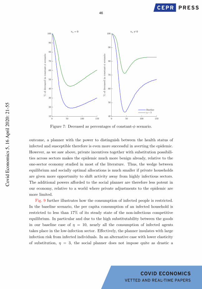
COVID ECONOMICS VETTED AND REAL-TIME PAPERS
Figure 7: Deceased as percentages of constant-φ scenario.
outcome, a planner with the power to distinguish between the health status of
infected and susceptible therefore is even more successful in averting the epidemic.
However, as we saw above, private incentives together with substitution possibili-
ties across sectors makes the epidemic much more benign already, relative to the
one-sector economy studied in most of the literature. Thus, the wedge between
equilibrium and socially optimal allocations is much smaller if private households
are given more opportunity to shift activity away from highly infectious sectors.
The additional powers afforded to the social planner are therefore less potent in
our economy, relative to a world where private adjustments to the epidemic are
more limited.
Fig. 9 further illustrates how the consumption of infected people is restricted.
In the baseline scenario, the per capita consumption of an infected household is
restricted to less than 17% of its steady state of the non-infectious competitive
equilibrium. In particular and due to the high substitutability between the goods
in our baseline case of η = 10, nearly all the consumption of infected agents
takes place in the low-infection sector. Effectively, the planner insulates with large
infection risk from infected individuals. In an alternative case with lower elasticity
of substitution, η = 3, the social planner does not impose quite as drastic a
46C
ovid
Eco
nom
ics 5
, 16
Apr
il 20
20: 2
1-55

COVID ECONOMICS VETTED AND REAL-TIME PAPERS
Figure 8: Heterogeneous-sector economy: social planning solution.
difference across the sectors (since this would be very costly in terms of lifetime
utility of the infected individuals, which the planner values), and rather lowers
the total consumption of the infected agent to around 20% of the non-infectious
steady state. In the homogeneous sector case, alternatively, the case for η = 0,
consumption in both sectors is the same, as the dotted-black line shows: now,
consumption for the infected is reduced to only 8 percent of the non-infectious
steady state. It is in this treatment of the infected, where the sectoral substitution
possibilities matter considerably.
One should take the social planner solution with a grain of salt, of course.
Presumably, a really powerful social planner would entirely separate the infected
and recovered people from the susceptible people. If this is technologically fea-
sible, the disease cannot spread any further, and no consumption decline for the
infected is needed. The formulation of our social planner problem precludes this
possibility. In summary, our calculations and this remark shows that the possi-
bility for containing the pandemic depends crucially on the tools available to the
government, and they may involve imposing considerable hardship on a few (the
initially infected) in order to rescue the many.
47C
ovid
Eco
nom
ics 5
, 16
Apr
il 20
20: 2
1-55

COVID ECONOMICS VETTED AND REAL-TIME PAPERS
Figure 9: Per capita consumption of infected people.
7 Conclusion
Our paper is inspired by the macroeconomics-cum-SIR model of Eichenbaum et al.
(2020). We depart from their analysis in that we permit substitution of consump-
tion across sectors with different degrees of infection probabilities. We show that
the resulting economic outcome differ dramatically as a result. With homogeneous
sectors, we obtain a steep decline of economic activity, fully in line with ERT. If the
substitution mechanism is activated, eighty percent of that decline is mitigated in
our benchmark calibration and in the decentralized economy: the “curve” is flat-
tened substantially, without much prolongation. Pushing the parameters a bit
more and thus capturing that people practice additional social distancing and hy-
giene, we show that infections may decline entirely on their own, simply due to
the re-allocation of economic activity: the curve does not just get flattened, it
gets reversed. One may view our results as the “Swedish” outcome: Sweden has
largely avoided government restrictions on economic activity, allowing people to
make their own choices. These private incentives and well-functioning labor-and-
social-insurance markets, we submit, may solve the COVID19-spread on their own,
mitigating the decline in economic activity.
48C
ovid
Eco
nom
ics 5
, 16
Apr
il 20
20: 2
1-55

COVID ECONOMICS VETTED AND REAL-TIME PAPERS
References
Adhmad, S. and D. Riker (2019, May). A method for estimating the elasticity
of substitution and import sensitivity by industry. Economics WOrking Paper
Series 2019-05-B, U.S. International Trade Commission.
Alvarez, F., D. Argente, and F. Lippi (2020, April). A simple planning problem
for covid-19 lockdown. Draft, University of Chicago.
Atkeson, A. (2020, March). What will be the economic impact of covid-19 in the
us? rough estimates of disease scenarios. NBER WP No. 26867.
Berger, D., K. Herkenhoff, and S. Mongey (2020). An seir infectious disease model
with testing and conditional quarantine. BFI Working Paper NO. 2020-25.
Correia, S., S. Luck, and E. Verner (2020, March). Pandemics depress the economy,
public health interventions do not: Evidence from the 1918 flu. Draft.
Dingel, J. and B. Neimann (2020). How many jobs can be done at home? Covid
Economics: Vetted and Real-Time Papers.
Eichenbaum, M., S. Rebelo, and M. Trabandt (2020, March). The macroeonomics
of epidemics. Draft, Northwestern University.
Fang, H., L. Wang, and Y. Yang (2020, March). Human mobility restrictions and
the spread of the novel coronavirus (2019-ncov) in china. Working Paper 26906,
National Bureau of Economic Research.
Fernandez-Villaverde, J. (2010). The econometrics of DSGE models. SERIEs 1,
3–49.
Glover, A., J. Heathcote, D. Kruger, and J.-V. Rios-Rull (2020, April). Health
versus wealth: On the distributional effects of controlling a pandemic. Draft.
Greenstone, M. and V. Nigam (2020). Does social distancing matter? (March 30,
2020). University of Chicago, Becker Friedman Institute for Economics Working
Paper No. 2020-26. Available at SSRN: https://ssrn.com/abstract=3561244 or
http://dx.doi.org/10.2139/ssrn.3561244.
Guerrieri, V., G. Lorenzoni, L. Straub, and I. Werning (2020, March). Macroe-
conomic implications of covid-19: Can negative supply shocks cause demand
shortages? Draft, MIT.
49C
ovid
Eco
nom
ics 5
, 16
Apr
il 20
20: 2
1-55

COVID ECONOMICS VETTED AND REAL-TIME PAPERS
Kaplan, G., B. Moll, and G. Violante (2020, March). Pandemics according to
HANK. Draft, University of Chicago.
Leibovici, F., A. M. Santacreu, and M. Famiglietti (2020). Social distancing and
contact-intensive occupations. On the economy, St. Louis FED .
Mongey, S. and A. Weinberg (2020, March). Characteristics of workers in low
work-from-home and high personal-proximity occupations. Draft, University of
Chicago.
50C
ovid
Eco
nom
ics 5
, 16
Apr
il 20
20: 2
1-55

COVID ECONOMICS VETTED AND REAL-TIME PAPERS
A Two-sector simulations
The consumer interaction indicator φ(k) is defined piece-wisely as
φ(k) =
φ1 k ∈ [0, υ)
φ2 k ∈ [υ, 1]
where υ is the size of the sector with lower consumer interactions. For each sector
j ∈ {1, 2}, there is a first-order condition with respect to cxjt, where x ∈ {s, i, r}.The equations for infected and recovered people are substituted out, because their
consumption and labor are constant. The following equations consist the system
delivering the paths of key variables.
υ1/η1
1cst
(cstcs1t
)1/η
=θ
Anst + πsItλτ,tφ1
A√θ
(A.1)
υ1/η2
1cst
(cstcs2t
)1/η
=θ
Anst + πsItλτ,tφ2
A√θ
(A.2)
cs1t + cs2t = Anst (A.3)
cst =[υ
1/η1 cs1t
1−1/η + υ1/η2 cs2t
1−1/η] ηη−1
(A.4)
λτ,t = −β(U it+1 − Ust+1
)(A.5)
Ust = u (cst , nst ) + β
[(1− τt)Ust+1 + τtU
it+1
](A.6)
U it = u(ci, ni
)+ β (1− πd)U it+1 (A.7)
τt =A√θπsIt (φ1c
s1t + φ2c
s2t) (A.8)
Tt = τtSt (A.9)
St = 1− It −Rt −Dt (A.10)
Rt = Rt−1 + πrIt−1 (A.11)
Dt = Dt−1 + πdIt−1 (A.12)
It = Tt−1 + (1− πd − πr) It−1 + 1t=1ε (A.13)
Note that the time convention of disease dynamics is modified for implementation
in Dynare. An MIT shock of size 0.001 is added to (A.13) in period 1. The paths
51C
ovid
Eco
nom
ics 5
, 16
Apr
il 20
20: 2
1-55
COVID ECONOMICS VETTED AND REAL-TIME PAPERS
of aggregate consumption and labor are given by
Ct = Stcst + (It +Rt)
A√θ
(A.14)
Nt = Stnst + (It +Rt)
1√θ
(A.15)
B Eliminating cstk
Note that citk = A/√θ. Let us reexamine (13) and write it as
(cstcstk
)1/η
= xtk (B.1)
where we define
xtk = cst
(λsbt + νtφ(k)A/
√θ)
(B.2)
Rewrite (B.1) as
cstk = x−ηtk cst (B.3)
Thus
(cstk)1−1/η = x1−ηtk (cst )
1−1/η (B.4)
and integrate∫(cstk)1−1/ηdk =
∫x1−ηtk dk × (cst )
1−1/η
Taking this to the power η/(η − 1) finally yields
cst =
(∫x1−ηtk dk
)η/(η−1)
cst
52C
ovid
Eco
nom
ics 5
, 16
Apr
il 20
20: 2
1-55

COVID ECONOMICS VETTED AND REAL-TIME PAPERS
or the constraint
1 =
(∫x1−ηtk dk
)η/(η−1)
This can be simplified to
1 =
∫x1−ηtk dk (B.5)
or
cst =
(∫ (λsbt + νtφ(k)A/
√θ)1−η
dk
)1/(1−η)
(B.6)
Thus, (4) and (5) can be rewritten as
τt = πsIt
∫φ(k)xηtkc
stA/√θdk (B.7)
= πsIt
∫φ(k)
(λsbt + νtφ(k)A/
√θ)−η
(cst )1−ηA/
√θdk (B.8)
and
Tt = πsStIt
∫φ(k)xηtkc
stA/√θdk (B.9)
= πsStIt
∫φ(k)
(λsbt + νtφ(k)A/
√θ)−η
(cst )1−ηA/
√θdk (B.10)
C Details of the Heterogeneous Labor Economy
To see the similarities and differences between the heterogeneous consumption-
and heterogeneous labor economy more formally, observe that the first order con-
ditions for infected and recovered agents are unchanged. In particular, we obtain
cit = citk ≡ A/√θ and nit = nitk = 1/
√θ, regardless as to whether consumption or
labor is heterogeneous. It therefore suffices to examine the first order conditions
for susceptible agents. Define relative consumption rtk = cstk/cst for the case of
heterogeneous consumption economy and qtk = nstk/nt for the case of the hetero-
geneous labor economy. Substituting out the Lagrange multiplier on the budget
constraint, one obtains a set of three equations for both economies: the combined
first-order conditions for consumption and labor, the aggregation constraint across
the sectors and the budget constraint. In the case of heterogeneous consumption
53C
ovid
Eco
nom
ics 5
, 16
Apr
il 20
20: 2
1-55
COVID ECONOMICS VETTED AND REAL-TIME PAPERS
and exploiting our knowledge regarding citk, these are
1
cstr−1/ηtk − θ
Anst = λτtIt
A√θπsφ(k)
1 =
∫r
1−(1/η)tk dk∫
rtkdk =Anstct
Multiply the first equation with rtk and integrate across k to find
1− θ(nst )2
cst= λτtIt
A√θπs
∫φ(k)rtkdk (C.1)
In the case of heterogeneous labor, denoting the infection parameter with πs
and again, exploiting our knowledge regarding nitk, we obtain
A
cst− θnstq
−1/ηtk = λτtIt
1√θπsφ(k)
1 =
∫q
1−(1/η)tk dk∫
qtkdk =ctAnst
Multiply the first equation with qtk and integrate across k to find
1− θ(nst )2
nst= λτtIt
1√θπs
∫φ(k)qtkdk (C.2)
Note that πs multiplies a term in units of squared labor rather than squared
consumption goods: it should naturally take a different value. One would get the
same solution for all aggregates in the heterogeneous labor case, given a solution
the heterogeneous consumption case, if it were the case that
πs = Acstnst
∫φ(k)rtkdk∫φ(k)qtkdk
Given that the right hand side depends on t and, additionally, given that qtk
depends on πs, one could seek an appropriate time-dependent sequence of πs to
make both models deliver the same aggregates.8.
8As an additional complication, Additionally, Jensens inequality implies that ct <∫ctkdk
and nt <∫ntkdk, provided ctk and ntk are not constant, creating an additional hurdle in the
appropriate adjustments and comparisons.
54C
ovid
Eco
nom
ics 5
, 16
Apr
il 20
20: 2
1-55

COVID ECONOMICS VETTED AND REAL-TIME PAPERS
D First Order Conditions of the Social Planner
Problem
The social planner’s problem in the main text yields the following first-order con-
ditions:(∂
∂cst:
)us1,t
(cstcstk
)1/η
+ µf,t = βπsφµI,t+1Itcitk(
∂
∂cit:
)ui1,t
(citcitk
)1/η
+ µf,t = βπsφµI,t+1Stcstk(
∂
∂crt:
)ur1,t
(crtcrtk
)1/η
+ µf,t = 0(∂
∂nst:
)us2,t = µf,tA(
∂
∂nit:
)ui2,t = µf,tA(
∂
∂nrt:
)ur2,t = µf,tA(
∂
∂St:
)u (cst , n
st ) + µf,t
∫cstkdk + µS,t = µf,tAn
st
+β
[µS,t+1 + µI,t+1πsIt
∫φ(k)cstkc
itkdk
](∂
∂It:
)u(cit, n
it
)+ µf,t
∫citkdk + µI,t = µf,tAn
it − µS,t
+β [(µS,t+1 + µI,t+1) (1− πr − πd)
+πrµR,t+1 + µI,t+1πsSt
∫φ(k)cstkc
itkdk
](
∂
∂Rt:
)u (crt , n
rt ) + µf,t
∫crtkdk + µR,t = µf,tAn
rt + βµR,t+1
55C
ovid
Eco
nom
ics 5
, 16
Apr
il 20
20: 2
1-55

COVID ECONOMICS VETTED AND REAL-TIME PAPERS
Covid Economics Issue 5, 16 April 2020
Global economic and financial effects of 21st century pandemics and epidemics1
Chang Ma,2 John Rogers3 and Sili Zhou4
Date submitted: 4 April 2020; Date accepted: 6 April 2020
We provide perspective on the possible global economic and financial effects from COVID-19 by examining the handful of similar major health crises in the 21st century. We estimate the effects of these disease shock episodes on GDP growth, fiscal policy, expectations, financial markets, and corporate activity. Simple time-series models of GDP growth indicate that real GDP is 2.6% lower on average across 210 countries in the year of the official declaration of the outbreak and is still 3% below its pre-shock level five years later. The negative effect on GDP is felt less in countries with more aggressive first-year responses in government spending. Consensus forecast data suggests a pessimistic view on real GDP initially that lasts for two months, an effect that is larger for emerging market economies. Stock market responses indicate an immediate negative reaction. Finally, using firm-level data, we find a fall in corporate profitability and employment, and an increase in debt, the last of which is further reflected in higher sovereign CDS spreads.
1 We are grateful for excellent research assistance provided by Caitlin Dutta and Jiqiao Gao. The views in this paper are solely the responsibility of the authors and should not be interpreted as reflecting the views of the Board of Governors of the Federal Reserve System or of any other person associated with the Federal Reserve System.
2 Assistant Professor of Finance, Fanhai International School of Finance, Fudan University.3 Senior Adviser, International Finance Division, Federal Reserve Board.4 Assistant Professor of Finance, Fanhai International School of Finance and School of Economics, Fudan
University.
56C
ovid
Eco
nom
ics 5
, 16
Apr
il 20
20: 5
6-78

COVID ECONOMICS VETTED AND REAL-TIME PAPERS
1 Introduction
As worldwide deaths attributed to the COVID-19 pandemic approach 100,000, while the virus contin-ues to spread, prospects for real economic activity and financial markets are equally funereal. Amidlock downs and shelter in place commands in the United States and abroad, Altig et al. (2020) reportthat the Atlanta Fed/Chicago Booth/Stanford Survey of Business Uncertainty (SBU) for March (con-ducted from March 9-20) signals a rapidly deteriorating outlook in which firms are bracing for a hugedeterioration in business activity. It is feared by the authors that even the very large negative effecton expected sales in the March survey might be too optimistic. Federal Reserve Bank of St. LouisPresident Bullard has urged the creation of a “National Pandemic Adjustment Period” (NPAP) whoseobjective is to reduce the level of real economic activity by roughly one-half, at least through 2020Q2,while making large fiscal transfers to households and firms. The St. Louis Fed has produced a rangeestimates for 2020Q2 U.S. unemployment whose mid-point is above 30%.1 Gourinchas (2020) sim-ilarly calls for massive fiscal interventions, which our results provide strong empirical support for,and outlines baseline scenarios that produce GDP growth rates in the United States of between -6.5%and -10% for 2020.2 Financial market volatility has been extraordinary, with days of double-digitpercentage declines in equity markets, the VIX above 80, and mny spreads reaching levels not seensince 2008.3
In response to the expanding crisis, President Trump signed into law on March 27 an historic $2trillion stimulus package to assist efforts to thwart the spread of COVID-19. Additional fiscal stimulusis being actively considered. The Federal Reserve announced on March 23, amid severe stress inseveral funding markets, that it is “Using its full range of authorities to provide powerful support forthe flow of credit to American families and businesses.”4 Outside the United States, fiscal policies haveexpanded nearly everywhere and central banks have enacted policies like those of the Fed. In addition,bountiful U.S. dollar swap lines have been created and tapped, and pledges of copious support havecome from the International Monetary Fund.5
1See https://www.bloomberg.com/news/articles/2020-03-22/fed-s-bullard-says-u-s-jobless-rate-may-soar-to-30-in-2qand https://www.stlouisfed.org/on-the-economy/2020/march/back-envelope-estimates-next-quarters-unemployment-rate.
2See also https://promarket.org/this-is-not-the-time-to-be-cautious-we-need-to-contain-the-economic-contagion-of-the-coronavirus/
3An impressive collection of outlook scenarios for several key measures of activity in the macroeconomy, corporatesector, and financial markets for the U.S. and abroad have been produced by scholars at the Becker-Friedman Institute. Seehttps://bfi.uchicago.edu/insight/blog/key-economic-facts-about-covid-19/.
4The initiatives include a dazzling array of credit facilities: Primary Market Corporate Credit Facility (PMCCF),Secondary Market Corporate Credit Facility (SMCCF), Commercial Paper Funding Facility (CPFF), Term Asset-BackedSecurities Loan Facility (TALF) and Main Street Business Lending Program, which support the flow of credit to consumersand small business, and the Money Market Mutual Fund Liquidity Facility (MMLF).
5See https://www.imf.org/en/Topics/imf-and-covid19.
57C
ovid
Eco
nom
ics 5
, 16
Apr
il 20
20: 5
6-78
COVID ECONOMICS VETTED AND REAL-TIME PAPERS
Related Conceptual Literature
Much of the uncertainty concerning estimates of the ultimate economic and financial effects fromthe COVID-19 pandemic stems from the unknown timing and severity of the virus.6 Atkeson (2020)analyzes disease scenarios that are designed to provide input into calculations of economic costs.He works with a Markov model of epidemic spread in which the population is divided into threecategories: being susceptible, actively infected, and no longer contagious. How an epidemic plays outover time is determined by the transition rates between these three states. Eichenbaum et al. (2020)emphasize that the severity of the recession will be exacerbated by people’s decisions to cut backon economic activity in order to reduce the severity of the epidemic and save lives. As the authorsemphasize, the optimal government containment policy saves thousands of lives but increases theseverity of the recession because infected people do not fully internalize the effect of their decisions onthe spread of the virus. Berger et al. (2020) focus on the role of testing and case-dependent quarantineduring a period of asymptomatic infection, and find that testing can result in a pandemic with smallereconomic losses while keeping the human cost constant, a result that they label “common sense”.
A Peek at Past Disease Episodes
To shed lights on current COVID-19 crisis event, we focus on five global pandemic and epidemicevents in the 21st century identified by Jamison et al. (2017): SARS in 2003, H1N1 in 2009, MERS in2012, Ebola in 2014 and Zika in 2016. Figure 1 plots monthly stock market returns for 81,000 firmsworldwide and sovereign credit default swap spreads for more than 30 countries, in event windowsaround the official declaration of a health crisis (see Table A.2). For each disease episode, we assignthe event month declared by WHO to be month zero. For each event, we divide all countries intotwo groups according to their ratio of disease cases to national population. We take the differencebetween the average value of the “more affected” country group and the “less affected” country group.We average the difference across our five disease episodes. In panel A, we plot the mean differencefor stock returns and in panel B the mean difference for sovereign CDS (in bps). The dashed linesrepresent one standard error relative to the average value. Stock return differences decline rapidly,going from (slightly) significantly positive to significantly negative within 5 months. For sovereignCDS spreads, the mean difference between groups rises and becomes significantly positive beginningone month before the official declaration.
Figure 2 plots the distribution of annual real GDP growth rates (%) for two separate country-yeargroups in the 210 countries in our sample (Table A.1). Group one is the growth rate in disease onsetyears of all affected countries, while group 2 is all other country-years (all countries in non-diseaseyears and unaffected countries in disease episode years). Average GDP growth in non-disease country-years (group 2) is 3.96%, but in health crisis episode years growth slows to an average of 0.77%. The
6Witness the gaping confidence bands around the detailed projections for U.S. states athttps://covid19.healthdata.org/projections. Leduc and Liu (2020) analyze how more general uncertainty surround-ing COVID-19 is transmitted, and estimate a persistent one percentage point rise in U.S. unemployment.
58C
ovid
Eco
nom
ics 5
, 16
Apr
il 20
20: 5
6-78

COVID ECONOMICS VETTED AND REAL-TIME PAPERS
Figure 1 Disease Episodes and Financial Markets
Panel A: Stock Market Panel B: Sovereign CDS Spreads
-5 -4 -3 -2 -1 0 1 2 3 4 5-0.03
-0.02
-0.01
0
0.01
0.02
-5 -4 -3 -2 -1 0 1 2 3 4 5-40
-20
0
20
40
60
80
NOTE: The figure plots stock market returns and credit spread of sovereign CDS around the event window. We denotewith 0 the month in which WHO officially declares pandemic or epidemic, In panel A, we take the difference between theaverage stock market return for most affected countries and the average stock market return for least affected countries, bydisease episode. We display the average difference across our five episodes. In panel B, we take the difference between theaverage credit spread (in bps) for most affected countries and average credit spread (in bps) for least affected countries, byepisode. We display the average difference across our five episodes. The mean difference is plotted in the solid line whilethe dashed lines are one standard error relative to the average value.
distribution of GDP growth during non-disease country-years is right-skewed, reflecting steady long-run global growth trends after World War II. However, during disease periods the GDP growth ratedistribution is left-skewed.
Contribution of Our Paper
With this background, we provide perspective on the possible global economic and financial effectsfrom COVID-19 by examining previous pandemics and epidemics in the 21st century. Our paper thuscomplements and broadens contemporaneous work by Barro et al. (2020) and Correia et al. (2020),who examine the impact of the Spanish flu of 1918-19. Using simple time-series models of GDPgrowth (Jorda (2005) and Cerra and Saxena (2008)), we find that real GDP is 2.6% lower on averageacross 210 countries in the year the outbreak is officially declared and remains 3% below pre-shocklevel five years later.7 We also document the effects on country groups based on geography and levelof development.
7Results from estimating an AR(4) process as in Cerra and Saxena (2008) are similar to the local projections and soare made available on request only.
59C
ovid
Eco
nom
ics 5
, 16
Apr
il 20
20: 5
6-78

COVID ECONOMICS VETTED AND REAL-TIME PAPERS
Figure 2 Real GDP Growth Distributions in Disease and Non-Disease Periods
0.0
5.1
.15
-10 0 10 20 -10 0 10 20
Normal Period Onset Years
Dens
ity
GDP growth (annual %)
NOTE: The distribution of real GDP growth rate (%) for onset years of the disease episodes (including all the affectedcountries) and normal periods (including all countries in other years and non-affected countries during the onset years ofthe disease episodes). The mean for the non-disease (disease) period is 3.96 (0.77). Standard deviations for the non-disease(disease) period is 5.81 (5.33); skewness is 4.24 (-0.26) and kurtosis 90.73 (4.23).
Importantly from the perspective of policy, we show that fiscal policy responds aggressively todisease outbreaks, with initial year declines of 2% of GDP in the primary surplus on average. Fur-thermore, we show that countries that respond more aggressively through higher government expendi-tures suffer smaller declines in output growth compared to countries with less of a fiscal expendituresresponse. The relative degree of tax policy response makes no difference, however. We also use con-sensus forecast data on real GDP growth and find that forecasts are overly optimistic concerning thenegative effect of the disease shock. On the other hand, stock market responses indicate that there is ashort-run over-reaction of the negative impact. Finally, using firm-level data, we find a prolonged con-traction from disease episodes, with a fall in corporate profitability and employment, and an increasein debt, which are consistent with the higher sovereign CDS spreads.
2 Methodology and Data
2.1 Estimation Method
To estimate the effect of major disease events on output, we follow Jorda (2005) and Cerra and Sax-ena (2008) to estimate impulse response functions to the health crisis shock. Given our large set ofcountries, we use panel data methods and partition the country samples in various ways to estimate
60C
ovid
Eco
nom
ics 5
, 16
Apr
il 20
20: 5
6-78

COVID ECONOMICS VETTED AND REAL-TIME PAPERS
differential effects on countries according to, e.g., their fiscal policy responses. Our baseline impulseresponse functions are estimated using the following equations as in Jorda (2005).8
H
∑h=0
git+h = αHi +
2
∑j=1
βHj git− j +
2
∑s=0
δHs Dit−s +Xit + εit ,with H = 0,1, · · · ,5. (1)
where git is the percentage change of real GDP for country i in year t, Dit is a dummy variable indicat-ing a pandemic/epidemic disease hitting country i in year t and Xit includes country-level controls forTrade/GDP, Domestic Credit/GDP, population and log GDP per capita. We also control for countryfixed effects. Standard errors are clustered at the country level. We display one standard error bandsaround the estimates.
We focus on the impulse response functions of cumulative growth rates from an unexpected shockto Dit at time t. Specifically, we plot the dynamics of {δH
0 }5H=0 for horizons up to five years after the
shock. Our results should thus be interpreted as the effect of a health crisis on the difference betweenoutput H years after the shock and output in the onset year of the shock.9
2.2 Data
We combine data from several sources. For the country-level analyses, we rely mainly on the WorldDevelopment Indicators (WDI) from the World Bank. We obtain forecasts of GDP growth from Con-sensus Economics Inc. and firm-level financial data from Thomson Reuters Worldscope. To identifythe pandemic and epidemic events, we manually collect data from the WHO and other public re-sources.
Epidemic and Pandemic Events
As noted above, we focus on five global pandemic and epidemic events in the 21st century identifiedby Jamison et al. (2017): SARS in 2003, H1N1 in 2009, MERS in 2012, Ebola in 2014 and Zika in2016. In each event, different sets of countries are affected differently. We collect data on total casesand deaths from the official websites of the World Health Organization (WHO), European Centre forDisease Prevention and Control (ECDC), Centers for Disease Control and Prevention (CDC) and frompublic news articles.
We identify a country as hit by the pandemic/epidemic event using the announcement date fromthe WHO. In most cases, there are significant time lags between the initial appearance of a pandemicoutbreak and official declaration. This likely explains why stock market returns and CDS spreads
8We are aware of the bias in impulse responses estimated by local projections with small sample sizes, especially inthe time dimension (Herbst and Johannsen (2020)).
9We use the STATA code on Jorda’s website. He estimates the effect of an interest rate shock onthe difference between output H periods after the shock and output in the onset period of the shock. Seehttps://sites.google.com/site/oscarjorda/home/local-projections. Cerra and Saxena (2008) looks at the effect of a finan-cial crisis on the difference between output H years after the shock and output in the onset year.
61C
ovid
Eco
nom
ics 5
, 16
Apr
il 20
20: 5
6-78

COVID ECONOMICS VETTED AND REAL-TIME PAPERS
seemingly react before the announcement of the event in Figure 1.10 For each event, we identify theset of affected countries and collect information on the number of deaths and cases reported for eachcountry. Among the five events, the most widespread and deadly one is H1N1 (Swine Flu Influenza).It affected more than 200 counties, with more than 284,000 recognized deaths reported by the USCDC, an amount that is 15 times larger than the number reported by WHO.11 In our analysis, we usethe number of deaths reported by the ECDC because it is the only one containing detailed informationfor all affected countries. Nevertheless, the reporting discrepancy between the CDC and the WHOdoes not affect our key identification variable — a dummy variable (i.e. the health crisis shock) thatequals one when WHO declares a pandemic/epidemic for the country, and zero otherwise. In oursample, we have have 290 country-year observations for the identified shocks. Detailed informationis in Table A.2.
Country-level Variables
We use real GDP growth rates from the World Bank’s World Development Indicators (WDI), whichcontains the 210 countries in Table A.1. The country-level data consists of unbalanced panels ofannual observations from 1960 to 2018. The key controls at the country level include trade to GDPratio, domestic credit to GDP, the natural log of national population, and the natural log of GDP percapita. Summary statistics are in Table A.4. All continuous variables are winsorized at the top andbottom 1% to remove outliers.
Forecasts of GDP growth in the current year and next year are obtained from Consensus EconomicsInc. The data are monthly, from a survey of expectations of analysts from large banks and financialfirms. We have data coverage over 32 countries from January 1990 to February 2020. We take theaverage of GDP growth expectations in the current year for each country-year and then merge it withthe actual GDP growth rates from the WDI database. The annual GDP surprise is calculated as takingthe difference between the actual GDP growth rates and the consensus forecasts.
Firm-level Variables
We collect firm-level data from Thomson Reuters Worldscope, which provides all the financial reportsfor over 81,000 listed companies in more than 120 countries.12 The database also provides historicaldata back to 1981, but includes listed firms in emerging countries only after 1990. Therefore, our
10For example, Hoffman and Silverberg (2018) find that the H1N1 outbreak initially began on March 15, 2009, wasdetected by officials on March 18, 2009, but was declared as a Public Health Emergency of International Concern (PHEIC)only on April 25, 2009. Similarly, the West African Ebola outbreak began December 26, 2013, was detected on March 22,2014, but was declared a PHEIC only on August 8, 2014. For Zika, the main concern was about identification betweenmicrocephaly and the true Zika virus infections. Hence, we consider this outbreak to have begun on October 22, 2015,when the rise in microcephaly cases was first identified. Later, on November 28, 2015, there was strong evidence for a linkbetween the virus and the microcephaly. Nevertheless, the Zika outbreak was declared a PHEIC only on February 1, 2016.
11Detailed information is provided here. http://www.cidrap.umn.edu/news-perspective/2012/06/cdc-estimate-global-h1n1-pandemic-deaths-284000
12Detailed information can be found at https://www.refinitiv.com/content/dam/marketing/en_us/documents/fact-sheets/fundamentals-worldscope-fact-sheet.pdf
62C
ovid
Eco
nom
ics 5
, 16
Apr
il 20
20: 5
6-78

COVID ECONOMICS VETTED AND REAL-TIME PAPERS
sample runs from 1990 to 2018. We exclude financial firms (SIC code: 6000 - 6999) because theyhave different disclosure regulations and their leverage positions are special compared to firms in othersectors. Our main firm-level measures include size (log of total assets in dollars), sales, investment(capital expenditures divided by assets), leverage (total debt divided by assets), tangibility (net prop-erty, plant and equipment divided by assets), cash (cash holdings divided by assets), ROA/ROE (netincome divided by assets/shareholder equity), Tobin’s Q (assets plus market value of equity and mi-nus book value of equity and divided by total assets), and labor to assets (employees divided by totalassets). Details construction are reported in Table A.3. All continuous variables are winsorized at thetop and bottom 1% to remove outliers.
3 Effect on Actual and Expected Real GDP
3.1 Real GDP: Impulse Response Functions
As seen in panel A of Figure 3, the global effect of a pandemic/epidemic event on output is negativeand highly persistent. The average loss in output is about 2.6 percent for the entire panel of countriesin the year of official declaration of the outbreak. Output is still 3 percent below the pre-shock levelfive years later. The global effect from H1N1 is slightly larger (panel B), with output loss of 4 percentin the first year and still 4.43 percent five years later. The output loss varies geographically, averaging3.15 percent for advanced economies (about one-third that amount for the Unites States), and 2.24percent for emerging market economies. Five years later, the output loss is 3.5 percent for advancedeconomies and 2.12 for emerging economies (see panels C and D). Output loss among the countriesof East Asia and South Asia is small and short-lived: 1.22 percent in the first year and recovered inthe second year. In contrast, output loss in Europe and Central Asia is large and persistent, around 5percent in the first year and beyond (panels E and F).
3.2 Real GDP: Panel Regressions
We estimate panel regressions for real GDP growth in Table 1. Column 1 displays results for the fullsample period 1960-2018, while the remaining columns are for 1990-2018 due to our use of consen-sus forecasts of current year GDP growth, which are available for 32 countries beginning in 1990.Specifications with the forecasts control for expectations, which essentially entirely account for theeffects of the economic control measures. Panel A includes all pandemic/epidemic events in the shockdummy while Panel B utilizes separate shock dummies for each episode. In Panel A, the coefficientson the shock dummy ranges from 2.65% to 3.52%, statistically significant and economically large. InPanel B, with five separate shock dummies, H1N1 has the largest effect, consistent with the impulseresponse functions. This is unsurprising because H1N1 affected the most countries and had the largestnumber of deaths and cases. Still, the effect of the other disease episodes is not negligible. In Table
63C
ovid
Eco
nom
ics 5
, 16
Apr
il 20
20: 5
6-78

COVID ECONOMICS VETTED AND REAL-TIME PAPERS
2, we replace our shock dummy by the ex-post mortality rate or affected rate for each country. Thecoefficients on both mortality rate and cases-to-population are negative and significant: countries thatsuffer either greater mortality or case infections suffer larger output losses.
3.3 Expectations of GDP Growth
We now consider how GDP growth expectations were affected by the onset of the disease episodes.We use the event month declared by WHO in Table A.2 as the onset year-month t for affected countryi for each disease event.13 Given the data availability, our panel regressions using consensus forecastsinclude only 32 countries, which are both advanced and emerging. In Table 3, we regress the change inthe monthly consensus forecast (Fg
ikt - Fgik−1t) on the disease shock dummy and its four lags, where Fg
ikt
denotes the consensus forecast of growth rate for country i at month k, year t. In addition to the countryfixed effects, we include month fixed effects to alleviate the potential seasonality of GDP growthforecasts (greater accuracy toward the end of the year). We find that disease episodes significantlylowers forecasts of GDP growth in the onset month. Furthermore, there is a persistent effect onexpectations lasting two months. We also find a larger and more pessimistic effects from diseases onforecasts of emerging market GDP growth rates.
4 Fiscal Policy
How does fiscal policy respond?
We explore the response of fiscal policy to the global pandemic/epidemic event in Figure 4. Followingthe disease shock, the primary surplus to GDP ratio falls by 1.91%, government revenues to GDP fallby 0.61%, and government expenditures rise by 1.25 % of GDP in the onset year. All responses areinsignificant by the third year after the shock.
Do tax cuts [no] or spending increases [yes] help?
Figure 5 displays the impulse responses of GDP growth, conditional on the fiscal response in the onset
year. We group countries into high and low government expenditures (or tax revenues) according toits change as percent of GDP in the onset year. We do this for each disease event, then average acrossthe five events. In countries with large responses of government expenditures, real GDP initially fallsby 2.68% but the effect dies out in the second year. For the low government expenditure responsecountries, real GDP initially falls by 2.84%, an effect that is very persistent. Meanwhile, responses ingovernment tax revenues do not make much of a difference.
13The WHO declarations are conservative on the late side, presumably due to concerns that Type I errors would lead toa loss of credibility such that the public would ignore future exhortations to caution.
64C
ovid
Eco
nom
ics 5
, 16
Apr
il 20
20: 5
6-78

COVID ECONOMICS VETTED AND REAL-TIME PAPERS
Figure 3 Effect on GDP: Impulse Response Functions
Panel A: Full Sample Panel B: H1N1
-6-5
-4-3
-2-1
01
2Percent
0 1 2 3 4 5Years
-6-5
-4-3
-2-1
01
2Percent
0 1 2 3 4 5Years
Panel C: Advanced Economies Panel D: Emerging Market Economies
-4.2
5-3
-2-1
01
2Pe
rcen
t
0 1 2 3 4 5Years
Advanced EconomiesUS
-4.25
-3-2
-10
12
Percent
0 1 2 3 4 5Years
Panel E: East Asia and South Asia Panel F: Europe and Central Asia
-6-5
-4-3
-2-1
01
23
4Percent
0 1 2 3 4 5Years
-6-5
-4-3
-2-1
01
23
4Percent
0 1 2 3 4 5Years
NOTE: Impulse response functions (IRF) are estimated based on the local projection method as in Jorda (2005) ∑Hh=0 git+h = αH
i +∑2j=1 βH
j git− j +
∑2s=0 δH
s Dit−s +Xit + εit ,with H = 0,1, · · · ,5, where git is the percentage change of real GDP for country i at year t, Dit is a dummy variable indicatinga disease event hitting country i in year t, with Xit including country-level controls such as Trade/GDP, Domestic Credit/GDP, population and log GDPper capita. We also control for country fixed effects. Standard errors are clustered at the country level. One standard error bands are shown. Panel A(B) presents full sample (for H1N1 only). Panel C (D) presents IRFs for the sample of advanced economies and the United States (emerging marketeconomies). Panel E (F) is for East Asia and South Asia (Europe and Central Asia).
65C
ovid
Eco
nom
ics 5
, 16
Apr
il 20
20: 5
6-78

COVID ECONOMICS VETTED AND REAL-TIME PAPERS
Table 1 The Effect of Pandemic Disease on Real GDP Growth: I
GDP growth rate %
Panel A
(1) (2) (3) (4)
Sample Period: 1960-2018 1990-2018
All Events All Events All Events Without H1N1
Shock -2.78*** -2.65*** -3.52*** -1.30**(0.28) (0.27) (0.58) (0.61)
Consensus Forecast 0.56*** 0.69***(0.16) (0.16)
Trade/GDP 0.00 0.01** -0.00 -0.00(0.00) (0.00) (0.01) (0.01)
Domestic Credit/GDP -0.02*** -0.03*** -0.02* -0.01(0.00) (0.01) (0.01) (0.01)
Log(Population) 0.14*** 0.06 0.08 0.07(0.04) (0.04) (0.13) (0.13)
Log(GDP per capita) -0.22** -0.02 -0.04 -0.03(0.09) (0.11) (0.26) (0.28)
Recession -0.29* -0.40** 0.05 0.52(0.16) (0.18) (0.48) (0.41)
Constant 4.86*** 4.74*** 2.48*** 2.04**(0.39) (0.44) (0.85) (0.79)
Observations 6647 4384 533 504Adjusted R-squared 0.055 0.064 0.207 0.166Decade FE Yes Yes Yes YesCountry FE Yes Yes Yes Yes
Panel B
(1) (2) (3) (4)
Sample Period: 1960-2018 1990-2018
All Events All Events All Events Without H1N1
EBOLA 0.90 0.58 -0.28 -0.34(0.62) (0.56) (0.37) (0.39)
H1N1 -4.41*** -4.27*** -5.32*** N.A.(0.39) (0.38) (0.72) N.A.
MERS -1.16* -0.94 -1.34 -1.23(0.69) (0.67) (1.50) (1.45)
SARS 0.15 0.01 -0.90** -0.94**(0.60) (0.58) (0.40) (0.41)
Zika -0.49 -0.51 -2.11*** -2.12**(0.41) (0.40) (0.76) (0.85)
Consensus Forecast 0.59*** 0.68***(0.16) (0.16)
Observations 6647 4384 533 504Adjusted R-squared 0.063 0.076 0.238 0.163Country Controls Yes Yes Yes YesDecade FE Yes Yes Yes YesCountry FE Yes Yes Yes Yes
NOTE: The dependent variable in column (1)-(4) is real GDP growth rate while the dependent variable. The sample periodfor column (1) is 1960-2018 while the sample period for column (2)-(4) is 1990-2018. Panel A reports Shock Dummy (allfive events), which equals to one for country i at onset year t, and zero otherwise. While Panel B replace Shock Dummywith five pandemics dummies. Each pandemic dummy is equal to one for country i at onset year t for outbreak of eachpandemic respectively. Country fixed effect is included. All standard errors are clustered at country level and reported inparentheses. ∗, ∗∗ and ∗∗∗ indicate statistical significance at the 10%, 5%, and 1% level, respectively.
66C
ovid
Eco
nom
ics 5
, 16
Apr
il 20
20: 5
6-78

COVID ECONOMICS VETTED AND REAL-TIME PAPERS
Table 2 The Effect of Pandemic Disease on Real GDP Growth: II
GDP growth rate %
(1) (2) (3) (4) (5) (6)
Sample Period: 1960-2018 1990-2018 1960-2018 1990-2018
Mortality Rate% -0.04*** -0.03*** -0.06**(0.01) (0.01) (0.02)
Cases/Pop(10 thousand) -3.40*** -3.22*** -5.64*(0.77) (0.75) (3.27)
Consensus Forecast 0.56*** 0.60***(0.16) (0.17)
Trade/GDP 0.00 0.01** 0.00 0.00 0.01** 0.00(0.00) (0.00) (0.01) (0.00) (0.00) (0.01)
Domestic Credit/GDP -0.02*** -0.04*** -0.02* -0.02*** -0.03*** -0.02*(0.00) (0.01) (0.01) (0.00) (0.01) (0.01)
Log(Population) 0.14*** 0.05 0.07 0.14*** 0.05 0.06(0.04) (0.04) (0.13) (0.04) (0.04) (0.14)
Log(GDP per capita) -0.23** -0.04 -0.05 -0.22** -0.03 -0.03(0.09) (0.11) (0.27) (0.09) (0.11) (0.28)
Recession -0.45*** -0.69*** -0.32 -0.42** -0.64*** -0.11(0.17) (0.18) (0.46) (0.16) (0.18) (0.45)
Constant 4.86*** 4.84*** 2.31** 4.85*** 4.80*** 2.13**(0.40) (0.45) (0.94) (0.40) (0.45) (0.92)
Observations 6638 4375 532 6641 4378 532Adjusted R-squared 0.041 0.043 0.111 0.044 0.047 0.135Decade FE Yes Yes Yes Yes Yes YesCountry FE Yes Yes Yes Yes Yes Yes
NOTE: The dependent variable in column (1)-(6) is real GDP growth rate while the dependent variable. The sample periodfor column (1) and (4) is 1960-2018 while the sample period for column (2)-(3) and (5)-(6) is 1990-2018. Country fixedeffect is included. All standard errors are clustered at country level and reported in parentheses. ∗, ∗∗ and ∗∗∗ indicatestatistical significance at the 10%, 5%, and 1% level, respectively.
67C
ovid
Eco
nom
ics 5
, 16
Apr
il 20
20: 5
6-78

COVID ECONOMICS VETTED AND REAL-TIME PAPERS
Figure 4 Response of Fiscal Policy
Panel A: Primary Surplus (% of GDP)-2
-1.5
-1-.5
0Percent
0 1 2 3 4 5Years
Panel B: Revenues (% of GDP) Panel C: Expenditures (% of GDP)
-1-.5
0.5
Percent
0 1 2 3 4 5Years
0.5
11.5
Percent
0 1 2 3 4 5Years
NOTE: Impulse response functions (IRF) are based on the local projection method of Jorda (2005): Yit+H −Yit−1 =αH
i +∑4j=1 βH
j Yit− j +∑4s=0 δH
s Dit−s +Xit−1 + εit , with H = 0,1, · · · ,5, where Yit is the primary surplus (or revenues orexpenditures) to GDP ratio for country i in year t, Dit is a dummy variable indicating a disease hitting country i in year tand Xit−1 includes country-level controls such as real GDP growth rate, population and log GDP per capita. The impulseresponse functions are shown with one standard error bands.
68C
ovid
Eco
nom
ics 5
, 16
Apr
il 20
20: 5
6-78

COVID ECONOMICS VETTED AND REAL-TIME PAPERS
Figure 5 Effect on GDP Growth Conditional on Immediate Fiscal Response
Panel A: Low Expenditure Response Panel B: High Expenditure Response
-5-4
-3-2
-10
1Percent
0 1 2 3 4 5Years
-5-4
-3-2
-10
1Percent
0 1 2 3 4 5Years
Panel C: Low Tax Response Panel D: High Tax Response
-5-4
-3-2
-10
1Percent
0 1 2 3 4 5Years
-5-4
-3-2
-10
1Percent
0 1 2 3 4 5Years
NOTE: Impulse response functions (IRF) are estimated based on the local projection method as in Jorda (2005):∑
Hh=0 git+h = αH
i +∑2j=1 βH
j git− j +∑2s=0 δH
s Dit−s +Xit + εit , with H = 0,1, · · · ,5, where git is the percentage change ofreal GDP for country i at year t, Dit is a dummy variable indicating a pandemic disease hitting country i in year t and Xitincludes country-level controls such as Trade/GDP, Domestic Credit/GDP, population and log GDP per capita. We alsocontrol for country fixed effects. Standard errors are clustered at the country level. We divide countries into two groupsbased on the average change of government expenditures (or tax revenues) normalized by GDP in the onset year of eachdisease event. One error bands are displayed. The shock is a one-time unexpected disease shock.
69C
ovid
Eco
nom
ics 5
, 16
Apr
il 20
20: 5
6-78
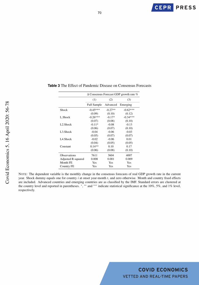
COVID ECONOMICS VETTED AND REAL-TIME PAPERS
Table 3 The Effect of Pandemic Disease on Consensus Forecasts
∆ Consensus Forecast GDP growth rate %
(1) (2) (3)
Full Sample Advanced Emerging
Shock -0.45*** -0.27** -0.62***(0.09) (0.10) (0.12)
L.Shock -0.26*** -0.17* -0.34***(0.07) (0.08) (0.10)
L2.Shock -0.11* -0.08 -0.13(0.06) (0.07) (0.10)
L3.Shock -0.04 -0.06 -0.03(0.05) (0.07) (0.07)
L4.Shock -0.02 -0.06 0.01(0.04) (0.05) (0.05)
Constant 0.14** 0.10 0.17(0.06) (0.08) (0.10)
Observations 7611 3604 4007Adjusted R-squared 0.008 0.001 0.009Month FE Yes Yes YesCountry FE Yes Yes Yes
NOTE: The dependent variable is the monthly change in the consensus forecasts of real GDP growth rate in the currentyear. Shock dummy equals one for country i at onset year-month t, and zero otherwise. Month and country fixed effectsare included. Advanced countries and emerging countries are as classified by the IMF. Standard errors are clustered atthe country level and reported in parentheses. ∗, ∗∗ and ∗∗∗ indicate statistical significance at the 10%, 5%, and 1% level,respectively.
70C
ovid
Eco
nom
ics 5
, 16
Apr
il 20
20: 5
6-78

COVID ECONOMICS VETTED AND REAL-TIME PAPERS
Table 4 The Effect of Pandemics on Firm-Level outcomes
ROA % Leverage % Labor/Assets % CAPX/Assets % TFP
(1) (2) (3) (4) (5) (6) (7) (8) (9) (10)
Shock -11.44*** -5.02*** 1.46*** 1.08*** -0.82*** -0.42*** 0.22 0.15 -0.34** -0.30(2.71) (1.74) (0.30) (0.27) (0.19) (0.15) (0.21) (0.15) (0.14) (0.19)
Log Assets 11.62*** 1.17*** -0.82*** 0.09*** -1.15***(3.00) (0.18) (0.18) (0.03) (0.07)
Cash 23.64*** -13.88*** -5.40*** 3.26*** -0.04(6.33) (2.05) (1.18) (0.56) (0.27)
Tobin’s Q -5.85*** 0.24*** 0.18*** 0.04*** -0.04***(0.75) (0.02) (0.03) (0.01) (0.01)
Sales Growth -1.40 0.26*** -0.15 0.36*** 0.15***(0.85) (0.08) (0.10) (0.03) (0.05)
Tangibility -2.36 11.61*** 0.98** 9.35*** -1.13***(2.23) (1.58) (0.49) (0.50) (0.20)
Constant 7.26 -233.47*** 14.02*** -15.18*** 11.19*** 27.44*** 8.00*** -0.86 -6.66*** 15.36***(12.12) (57.82) (1.25) (4.21) (2.88) (5.31) (0.60) (0.55) (1.17) (1.39)
Observations 833104 583912 812560 572794 580738 437714 786131 561511 565426 435269Adjusted R-squared 0.081 0.312 0.114 0.204 0.296 0.403 0.121 0.213 0.395 0.533Country FE Yes Yes Yes Yes Yes Yes Yes Yes Yes YesIndustry FE Yes Yes Yes Yes Yes Yes Yes Yes Yes YesYear FE Yes Yes Yes Yes Yes Yes Yes Yes Yes Yes
NOTE: This table reports estimated effects of disease episodes on firm-level outcomes between 1990 and 2018. Shock dummy equals one for firms headquartered at countryi with an outbreak year t, and zero otherwise. The firm characteristics are defined in Table A.3. We include industry fixed effects (by SIC 2digit code), country fixed effects,and year fixed effects. Standard errors are clustered at the country level and reported in parentheses. ∗, ∗∗ and ∗∗∗ indicate statistical significance at the 10%, 5%, and 1% level,respectively.
71C
ovid
Eco
nom
ics 5
, 16
Apr
il 20
20: 5
6-78

COVID ECONOMICS VETTED AND REAL-TIME PAPERS
5 Effects on Firms
Finally, we exam the effect of the disease episodes on firms. Our outcome variables are ROA (returnon assets), leverage (total debt to assets), labor to assets (number of employee to assets), investment(CAPEX expenditure to assets), and total factor productivity (TFP). In addition to standard firm-levelcontrols in our panel regression, we include industry fixed effect (SIC 2 digit code), country fixedeffects and year fixed effects. The variable of interest is the disease shock dummy, which equals onefor a firm when it is headquartered in country i at onset year t, and zero otherwise. Table 4 reports theresults. As seen in columns 1 and 2, ROA is significantly lower for firms located in affected countriesduring the disease year compared to those remained out during the normal period. The leverage ratiois also significantly higher. Moreover, we also find a significantly lower employment for firms affectedby the disease. But we do not find significant evidence for those firms to lower investment and thusTFP.
6 Conclusion
We estimate the effects of major global disease outbreaks in the 21st century on GDP growth, fiscalpolicy, expectations, financial markets, and corporate activity for a large cross-section of countries andfirms. We find that real GDP growth falls persistently, an effect that is felt more in countries with a lessaggressive first-year response in government spending. Consensus forecast data on real GDP growthindicates that private sector forecasts are underly pessimistic initially. On the other hand, stock marketresponses indicate a short-run over-reaction of the negative impact. Using firm-level data, we find afall in corporate profitability and employment, and an increase in debt. These financial developmentsare consistent with the documented higher sovereign CDS spreads.
It is difficult to translate these estimated historical effects to forecast the economic and financialeffects of COVID-19. Although there are many parallels between these 21st century disease episodesand COVID-19, there is a lot to suggest that this pandemic will have a much larger toll on humanlives. The unprecedented scale of lock downs in several countries will hamper economic activity evenfor countries that have lower case loads and deaths and/or who thwart the virus more quickly. Inthe disease episodes documented in this paper, U.S. GDP does not fall a lot by historical standards,but there are reasons to think that COVID-19 will be considerably more recessionary. For one, U.S.fiscal space is relatively limited now. If fiscal policy does not move enough, or with the right mix,COVID-19 will have a very persistent effect on output. We have shown that past disease episodeshave significant effects on firms (and surely households, something we do not directly address): loweremployment, lower profits, and higher leverage in the aftermath of health crises do not give optimismfor a steep and rapid recovery. Thus, we consider our estimates to be a lower bound for the case ofCOVID-19.
72C
ovid
Eco
nom
ics 5
, 16
Apr
il 20
20: 5
6-78

COVID ECONOMICS VETTED AND REAL-TIME PAPERS
References
ALTIG, D., J. M. BARRERO, N. BLOOM, S. J. DAVIS, B. MEYER, E. MIHAYLOV, AND N. PARKER
(2020): “American Firms Foresee a Huge Negative Impact of the Coronavirus,” Tech. rep., FederalReserve Bank of Atlanta, https://www.frbatlanta.org/blogs/macroblog/2020/03/23/american-firms-foresee-a-huge-negative-impact-of-the-coronavirus.
ATKESON, A. (2020): “What Will Be the Economic Impact of COVID-19 in the US? Rough Estimatesof Disease Scenarios,” Tech. rep., National Bureau of Economic Research, 26867.
BARRO, R. J., J. F. URSUA, AND J. WENG (2020): “The Coronavirus and the Great InfluenzaPandemic: Lessons from the “Spanish Flu” for the Coronavirus’s Potential Effects on Mortality andEconomic Activity,” Tech. rep., National Bureau of Economic Research, 26866.
BERGER, D. W., K. F. HERKENHOFF, AND S. MONGEY (2020): “An SEIR Infectious DiseaseModel with Testing and Conditional Quarantine,” Tech. rep., National Bureau of Economic Re-search, 26901.
CERRA, V. AND S. C. SAXENA (2008): “Growth dynamics: the myth of economic recovery,” Ameri-
can Economic Review, 98, 439–57.
CORREIA, S., S. LUCK, AND E. VERNER (2020): “Pandemics Depress the Economy,Public Health Interventions Do Not: Evidence from the 1918 Flu,” Tech. rep., SSRN-http://dx.doi.org/10.2139/ssrn.3561560.
EICHENBAUM, M. S., S. REBELO, AND M. TRABANDT (2020): “The Macroeconomics of Epi-demics,” Tech. rep., National Bureau of Economic Research, 26882.
GOURINCHAS, P. O. (2020): “Flattening the pandemic and recession curves,” Tech.rep., https://drive.google.com/file/d/1mwMDiPQK88x27JznMkWzEQpUVm8Vb4WI/view?usp=sharing.
HERBST, E. P. AND B. K. JOHANNSEN (2020): “Bias in Local Projections,” Tech. rep., Finance andEconomics Discussion Series 2020-010. Washington: Board of Governors of the Federal ReserveSystem, https://doi.org/10.17016/FEDS.2020.010.
HOFFMAN, S. J. AND S. L. SILVERBERG (2018): “Delays in global disease outbreak responses:lessons from H1N1, Ebola, and Zika,” American journal of public health, 108, 329–333.
JAMISON, D., H. GELBAND, S. HORTON, P. JHA, R. LAXMINARAYAN, C. MOCK, AND R. NU-GENT (2017): “Disease Control Priorities: Improving Health and Reducing Poverty,” .
JORDA, O. (2005): “Estimation and inference of impulse responses by local projections,” American
Economic Review, 95, 161–182.
73C
ovid
Eco
nom
ics 5
, 16
Apr
il 20
20: 5
6-78

COVID ECONOMICS VETTED AND REAL-TIME PAPERS
LEDUC, S. AND Z. LIU (2020): “The Uncertainty Channel of the Coronavirus,” Tech. rep., FederalReserve Bank of San Francisco Economic Letter, 2020-07.
74C
ovid
Eco
nom
ics 5
, 16
Apr
il 20
20: 5
6-78

COVID ECONOMICS VETTED AND REAL-TIME PAPERS
Table A.1 List of Countries from WDI (Total Number: 210)
Aruba Bolivia Dominica Grenada Kiribati Malta Papua New Gu Slovak Repub Venezuela, RAfghanistan Brazil Denmark Greenland St. Kitts an Myanmar Poland Slovenia British VirgAngola Barbados Dominican Re Guatemala Korea, Rep. Montenegro Puerto Rico Sweden Virgin IslanAlbania Brunei Darus Algeria Guam Kuwait Mongolia Korea, Dem. Eswatini VietnamAndorra Bhutan Ecuador Guyana Lao PDR Mozambique Portugal Seychelles VanuatuUnited Arab Botswana Egypt, Arab Hong Kong SA Lebanon Mauritania Paraguay Syrian Arab SamoaArgentina Central Afri Eritrea Honduras Liberia Mauritius West Bank an Turks and Ca Yemen, Rep.Armenia Canada Spain Croatia Libya Malawi French Polyn Chad South AfricaAmerican Sam Switzerland Estonia Haiti St. Lucia Malaysia Qatar Togo ZambiaAntigua and Chile Ethiopia Hungary Liechtenstei Namibia Romania Thailand ZimbabweAustralia China Finland Indonesia Sri Lanka New Caledoni Russian Fede TajikistanAustria Cote d’Ivoir Fiji India Lesotho Niger Rwanda TurkmenistanAzerbaijan Cameroon France Ireland Lithuania Nigeria Saudi Arabia Timor-LesteBurundi Congo, Dem. Faroe Island Iran, Islami Luxembourg Nicaragua Sudan TongaBelgium Congo, Rep. Micronesia, Iraq Latvia Netherlands Senegal Trinidad andBenin Colombia Gabon Iceland Macao SAR, C Norway Singapore TunisiaBurkina Faso Comoros United Kingd Israel Morocco Nepal Solomon Isla TurkeyBangladesh Cabo Verde Georgia Italy Monaco Nauru Sierra Leone TuvaluBulgaria Costa Rica Ghana Jamaica Moldova New Zealand El Salvador TanzaniaBahrain Cuba Gibraltar Jordan Madagascar Oman San Marino UgandaBahamas, The Cayman Islan Guinea Japan Maldives Pakistan Somalia UkraineBosnia and H Cyprus Gambia, The Kazakhstan Mexico Panama Serbia UruguayBelarus Czech Republ Guinea-Bissa Kenya Marshall Isl Peru South Sudan United StateBelize Germany Equatorial G Kyrgyz Repub North Macedo Philippines Sao Tome and UzbekistanBermuda Djibouti Greece Cambodia Mali Palau Suriname St. Vincent
75C
ovid
Eco
nom
ics 5
, 16
Apr
il 20
20: 5
6-78

COVID ECONOMICS VETTED AND REAL-TIME PAPERS
Table A.2 List of Global Pandemic and Epidemic Events
Starting Year Announced Month Event Name Affected Countries (Cities) Number of Countries Total Deaths Total Cases Mortality Rate2003 2 SARS AUS, CAN, CHE, CHN, DEU, ESP, FRA, GBR, HKG, IDN,
IND, IRL, ITA, KOR, KWT, MAC, MNG, MYS, NZL, PHL,ROU, RUS, SGP, SWE, THA, TWN, USA, VNM, ZAF
29 774 8096 9.56%
2009 4 H1N1 ABW, AFG, AGO, AIA, ALB, AND, ANT, ARE, ARG, ARM,ASM, ATG, AUS, AUT, AZE, BDI, BEL, BES, BGD, BGR,BHR, BHS, BIH, BLR, BLZ, BMU, BOL, BRA, BRB, BRN,BTN, BWA, CAN, CHE, CHL, CHN, CIV, CMR, COD, COG,COK, COL, CPV, CRI, CUB, CYM, CYP, CZE, DEU, DJI,DMA, DNK, DOM, DZA, ECU, EGY, ESP, EST, ETH, FIN,FJI, FLK, FRA, FSM, GAB, GBR, GEO, GGY, GHA, GIB,GLP, GRC, GRD, GTM, GUF, GUM, GUY, HND, HRV, HTI,HUN, IDN, IMN, IND, IRL, IRN, IRQ, ISL, ISR, ITA, JAM,JEY, JOR, JPN, KAZ, KEN, KHM, KIR, KNA, KOR, KWT,LAO, LBN, LBY, LCA, LIE, LKA, LSO, LTU, LUX, LVA,MAF, MAR, MCO, MDA, MDG, MDV, MEX, MHL, MKD,MLI, MLT, MMR, MNE, MNG, MOZ, MSR, MTQ, MUS,MWI, MYS, MYT, NAM, NCL, NGA, NIC, NLD, NOR,NPL, NRU, NZL, OMN, PAK, PAN, PER, PHL, PLW, PNG,POL, PRI, PRK, PRT, PRY, PSE, PYF, QAT, RKS, ROU, RUS,RWA, SAU, SDN, SGP, SLB, SLV, SOM, SRB, STP, SUR,SVK, SVN, SWE, SWZ, SYC, SYR, TCA, TCD, THA, TJK,TLS, TON, TTO, TUN, TUR, TUV, TZA, UGA, UKR, URY,USA, VCT, VEN, VGB, VNM, VUT, WLF, WSM, YEM,ZAF, ZMB, ZWE
201 14633a 529622 2.76%
2012 3 MERS ARE, AUT, CHN, DEU, DZA, EGY, FRA, GBR, GRC, IRN,ITA, JOR, KOR, KWT, LBN, MYS, NLD, OMN, PHL, QAT,SAU, THA, TUN, TUR, USA, YEM
26 498 1289 38.63%
2014b 8 Ebola ESP, GBR, GIN, ITA, LBR, MLI, NGA, SEN, SLE, USA 10 11323 28646 39.53%2016c 2 Zika ABW, AIA, ARG, ATG, BES, BHS, BLM, BLZ, BMU, BOL,
BRA, BRB, CAN, CHL, COL, CRI, CUB, CYM, DMA,DOM, ECU, GLP, GRD, GTM, GUF, GUY, HND, HTI, JAM,KNA, LCA, MAF, MSR, MTQ, NIC, PAN, PER, PRI, PRY,SLV, SUR, SXM, TCA, TTO, URY, USA, VCT, VEN, VGB,VIR
50 20 203094 0.01%
aThis estimates are from European Center for Disease Prevention and Controls (ECDC). We use their estimates since they provides detailed coverage and mortalityrate for each country. Detailed information can be found here: https://en.wikipedia.org/wiki/2009_flu_pandemic_by_country. However, the estimate from USCenters for Disease Control and Prevention (CDC) for global death troll is 284,000, about 15 times more than the number of laboratory-confirmed cases. See details inhttp://www.cidrap.umn.edu/news-perspective/2012/06/cdc-estimate-global-h1n1-pandemic-deaths-284000.
bThe West African Ebola outbreak began December 26, 2013 and was declared a PHEIC August 8, 2014.cThe Zika virus outbreak occurred at October, 2015 but was declared a PHEIC February 1, 2016
76C
ovid
Eco
nom
ics 5
, 16
Apr
il 20
20: 5
6-78

COVID ECONOMICS VETTED AND REAL-TIME PAPERS
Table A.3 Firm-level Variables
Variable Description Source
Size Logarithmic value of total assets(Worldscope item02999) WorldscopeSales Sales in thousands of dollars (Worldscope item 01001). WorldscopeInvestment Capital expenditures (Worldscope item 04601) divided by as-
sets (Worldscope item 02999).Worldscope
Leverage Total debt (Worldscope item 03255) divided by assets (World-scope item 02999).
Worldscope
Tangibility Net property, plant, and equipment (Worldscope item 02501)divided by assets (Worldscope item 02999).
Worldscope
Cash Cash holdings (Worldscope item 02001) divided by assets(Worldscope item 02999).
Worldscope
ROA Net income (Worldscope item 01751) scaled by total assets(Worldscope item 02999)
Worldscope
ROE Net income (Worldscope item 01751) scaled by shareholderequity (Worldscope item 03451+Worldscope item 03501).
Worldscope
Tobin’s Q Assets (Worldscope item 02999) plus market value of equity(Worldscope item 08001) minus book value of equity (World-scope item 03501) divided by total assets.
Worldscope
Capital/Labor Net property, plant, and equipment (Worldscope item 02501)divided by the number of employees (Worldscope item 07011).
Worldscope
Labor/Assets Number of employees (Worldscope item 07011) divided by as-sets.
Worldscope
TFP Calculated by log(Sales)-log(Assets)-log(Number ofEmployee)-log(Materials)
Authors’ own calculation
77C
ovid
Eco
nom
ics 5
, 16
Apr
il 20
20: 5
6-78

COVID ECONOMICS VETTED AND REAL-TIME PAPERS
Table A.4 Country-level Data: Summary Statistics
N Mean P50 S.D. P75 P25
GDP growth rate % 9,201 3.79 3.80 4.54 6.00 1.00Trade/GDP % 8,288 66.59 59.00 43.55 88.00 37.00Domestic Credit/GDP % 7,627 33.26 23.00 31.28 45.00 12.00Log(Population) 12,320 8.26 4.28 5.95 15.05 3.37Log(GDP per capita) 9,202 5.98 5.67 2.82 8.47 3.40
78C
ovid
Eco
nom
ics 5
, 16
Apr
il 20
20: 5
6-78

COVID ECONOMICS VETTED AND REAL-TIME PAPERS
Covid Economics Issue 5, 16 April 2020
Visualising and forecasting Covid-191
Albrecht Ritschl2
Date submitted: 6 April 2020; Date accepted: 8 April 2020
As an alternative to structural estimates of the SIR model, this note presents reduced-form time series forecasts of the growth in Covid-19 cases s and fatalities d for several countries where a slowdown has set in. Once a daily threshold of d >100 was crossed, daily growth in the initial unchecked phase was around Δln(d) ∈ [0.2,0.3]. For several countries, growth in fatalities as well as registered cases now shows a sustained decline; Italy and Spain report Δln(d) ≈ 0.03. I present updated ETS forecasts of the endpoint to the current epidemic for the countries in the sample, along with predicted fatalities. As a robustness check, forecasts from 31 March alongside later realizations are included. Results are preliminary and subject to daily revision as the situation is still evolving rapidly. The relative success of the method suggests univariate forecasts as a quick way of assessing resource needs and timelines where the epidemic is still ongoing.
1 Original version submitted April 7. Thanks are due to Alexander Ludwig and Harald Uhlig for comments on the first draft of March 30.
2 Professor of Economic History, LSE and CEPR Research Fellow.
79C
ovid
Eco
nom
ics 5
, 16
Apr
il 20
20: 7
9-10
5

COVID ECONOMICS VETTED AND REAL-TIME PAPERS
I. Introduction
Epidemiologists have a long tradition of modeling the spread of epidemics empirically. Their standard workhorse model SIR is well established, and widely accepted calibrations exist. However, adjustment and fine tuning to individual case studies poses problems of parameter calibration or estimation that can act as a short term obstacle to forecasting from the model whilst the situation is evolving, see the discussion in [1], [2], [3]. Publication of a study by Ferguson et al. [4] in March 2020 led to policy reversals towards the nascent Sars-Cov-2 epidemic in several countries on the basis of parameter revisions suggested in that study. Whilst attempts have been made in several countries to improve the collection and reporting of hospital micro data, see e.g. [5] for Britain or [6] for Germany, parameter uncertainty still appears to be rampant, especially in a cross-country perspective. Structural estimation of the SIR model in the presence of policy intervention is also susceptible to the Lucas critique. Substantial efforts are being directed towards influencing the behaviour of the public towards the spread of the infection. Medical resources are diverted from other uses to cope with an increased demand for intensive care services. All this is designed to affect both the infection and recovery rate, and would distort the Country and regional data collected and published daily [7] include reported fatalities, cases, and recoveries, often collected under widely different and often changing national or indeed local standards. Indicators that are often critically missing from this panel are capacity of and admissions to intensive care units, the length of stay at these units, and the survival probabilities of patients. It is this area where hospital micro data are often being employed in an attempt to complete the picture. However, these are snapshots, often still based on very limited case numbers.
Economists have acted quickly to close the gap between epidemiological and macroeconomic modeling, see e.g. Romer [8], Eichenbaum, Rebelo and Trabandt [9], Donsimoni et al. [10], Gros, Valenti, Valenti, and Gros [11] and Stock [12]. These approaches are primarily concerned with understanding and quantifying the transmission mechanisms between the epidemic and macroeconomic activity, aiming to model optimal policy responses. In a sense, these models are taking the epidemiologic part off the shelf, as their focus is on the implications.
The current note aims to contribute towards closing the gap, tackling the epidemiological forecasting issue with the toolbox of the economists, reduced-form time series forecasts. Absent reliable estimates of the underlying structural epidemiological parameters, the best a forecaster can hope for in the short run is to rely on univariate time series dynamics.
As epidemics are understood to follow logistic functions, there are obvious univariate time series characteristics to be exploited. After initial exponential growth, indicators of interest such as the growth rates in case and fatality numbers would enter into a slowdown, converging back to zero. As the number of observations grows during the slowdown period, estimates of the speed of convergence, endpoint times, as well as levels can be obtained. This is what the following note does.
80C
ovid
Eco
nom
ics 5
, 16
Apr
il 20
20: 7
9-10
5

COVID ECONOMICS VETTED AND REAL-TIME PAPERS
Focusing on univariate time series characteristics implies discarding the information that is potentially included in the dynamic relationships between the variables of interest. Noticeably, recorded cases should lead fatalities. In an ideal world where cases are identified upon infection, the lag should cover both the incubation period and of manifest illness itself. In practice, however, substantial recognition lags may exist, and testing practices may bias the lag. Whilst in some countries, tests are typically only carried out upon arrival to a hospital’s intensive care unit, in other countries more widespread testing is adopted, in the hope of covering a wider range of the population and of isolating identified cases. These national policies give rise to strong country effects in case reporting, which may or may not be fixed.
The discussions below are structured as follows. The next section provides an overview of recorded growth in fatalities in our sample. Reporting has been restricted to countries where both reported cases and reported fatalities have exceeded a minimum threshold of 100 cases. It is only beyond this threshold that reporting practices appear to be standardized and volatility in the reported figures is reduced to more plausible levels. The aim of the section is to provide stylized facts and identify those countries that have crossed the minimum threshold already. Section III turns to doubling times in fatalities, a metric that appears to have been more widely reported in the media than fatality growth, except for the very recent days. Section IV examines the relationship between fatalities and total cases. This turns out to be a non-linear relationship in most countries, and we obtain a rather clear representation of lower and upper bounds. Section V then presents forecasts for the end of the epidemic, as well as predicted levels of cumulative cases and fatalities. For most countries in our sample, the endpoint of the epidemic is predicted for the current month, although in many estimates there is considerable probability mass towards end of that timeline. We also identify countries where evidence of a slowdown is still shaky as of the time this note is completed. Section VI finally takes a brief look at hindcasts, i.e. forecasts as of March 31 compared with later realizations. The relative stability of these forecasts suggests the suitability of this simple tool for other cases where the epidemic is still ongoing. All results should nevertheless be received with caution, as the situation continues to evolve fast.
II. Fatalities: growth
Overall fatalities from Covid-19 are per se not the most pressing concern of politics, as total mortality when averaged out over a year might well be within the normal variations. What makes fatalities relevant is their close relationship to the burden of Covid-19 on hospitals’ intensive care units (ICUs). Small-sample clinical data from England and Wales [5] suggest that of Covid-related admissions (N=165) to ICUs, 58% require heavy respiration, and that among those under heavy respiration the survival rate is only 33%. Among patients aged 70 and over (N=56) the overall survival rate is only 26%.
Fatalities related to Covid-19 are available in levels [7] and widely reported in logs. Figure 1 instead provides a representation in log differences, an approximation to daily percentage growth in fatalities. The initial observations up to 𝑑𝑑 = 100 are omitted, as reporting habits and
81C
ovid
Eco
nom
ics 5
, 16
Apr
il 20
20: 7
9-10
5

COVID ECONOMICS VETTED AND REAL-TIME PAPERS
regulations have only typically stabilized at (sometimes much) higher levels. The evidence is grouped into three panels. Panel (a) includes Italy and Spain, the two Mediterranean countries strongly affected by Covid-19. Panel (b) includes Western European countries from Switzerland to the UK. Panel (c) provides data Germany, the State of New York including New York City, and also on the Hubei province of China, which includes the city of Wuhan where the virus was first identified.
Figure 1 (a) Southern Europe
Both countries present a combination of high pressure on their ICU capacities – more on this later – and a sustained slowdown in the growth of fatalities during the past weeks from ∆ ln(𝑑𝑑) ≈ 0.3 to ∆ ln(𝑑𝑑) ≈ 0.03 . There is noticeable volatility in the data during the early periods, which is a general pattern for almost all the countries studied here.
Italy has been under progressively tighter lockdowns since February. On February 21, a set of towns in the Northern region of Lombardy was quarantined. On March 8, the quarantine was extended to the whole of Lombardy and later to all of Italy. Spain imposed school closures and progressively strict lockdowns beginning March 12. These measures could only have a visible effect after 14 days or more. While they seem to have consolidated the slowdown, some evidence is already visible earlier.
00.10.20.30.40.50.60.70.80.9
1
21-F
eb
28-F
eb
6-M
ar
13-M
ar
20-M
ar
27-M
ar
3-Ap
r
10-A
pr
Covid- 19 fatalities Italylog diffs
00.10.20.30.40.50.60.70.80.9
1
4-M
ar
11-M
ar
18-M
ar
25-M
ar
1-Ap
r
8-Ap
r
Covid-19 fatalities Spainlog diffs
82C
ovid
Eco
nom
ics 5
, 16
Apr
il 20
20: 7
9-10
5

COVID ECONOMICS VETTED AND REAL-TIME PAPERS
Figure 1 (b) Western Europe
All countries in Figure 1 (b) were relative latecomers to the crisis, the Netherlands more so than the others. Reporting seems unreliable at times, with spurious-looking zero-fatality days occurring up until mid-March. The French figures include deaths in old age homes from April [13], shown separately in the Figure, whereas the UK data appear to leave out fatalities in care homes. In all countries, a downward trend in fatality growth has emerged, including now in the UK. Policies towards Covid-19 have varied considerably across Western Europe, which makes the evidence remarkable. France embarked on strict lockdowns earlier than the other countries in the figure. The UK and to some extent Switzerland changed course from an initial laissez-faire approach (“herd immunity”) to stricter measures. The elephant in the Western European room is the Netherlands, though, which has stuck to the herd immunity approach, apparently without having suffered worse outcomes. Unobserved heterogeneity and the implicit protection of the Netherlands through stricter measures elsewhere may play a role, although an argument
00.10.20.30.40.50.60.70.80.9
1
3-M
ar
10-M
ar
17-M
ar
24-M
ar
31-M
ar
7-Ap
r
14-A
pr
Covid-19 fatalities Switzerlandlog diffs
00.10.20.30.40.50.60.70.80.9
1
3-M
ar
10-M
ar
17-M
ar
24-M
ar
31-M
ar
7-Ap
r
14-A
pr
Covid-19 fatalities Francelog diffs
00.10.20.30.40.50.60.70.80.9
1
20-M
ar22
-Mar
24-M
ar26
-Mar
28-M
ar30
-Mar
1-Ap
r3-
Apr
5-Ap
r7-
Apr
9-Ap
r11
-Apr
13-A
pr
Covid-19 fatalities Netherlandslog diffs
00.10.20.30.40.50.60.70.80.9
1
3-M
ar
10-M
ar
17-M
ar
24-M
ar
31-M
ar
7-Ap
r
14-A
pr
Covid- 19 fatalities UKlog diffs
83C
ovid
Eco
nom
ics 5
, 16
Apr
il 20
20: 7
9-10
5

COVID ECONOMICS VETTED AND REAL-TIME PAPERS
for structural similarities between the Netherlands and Switzerland could be made. Yet outcomes across the two countries seem markedly different.
Figure 1 (c) Others
00.10.20.30.40.50.60.70.80.9
1
24-Ja
n
31-Ja
n
7-Fe
b
14-F
eb
21-F
eb
28-F
eb
6-M
ar
13-M
ar
20-M
ar
27-M
ar
3-Ap
r
Covid- 19 fatalities Hubei (China)log diffs
00.10.20.30.40.50.60.70.80.9
1
9-M
ar
16-M
ar
23-M
ar
30-M
ar
6-Ap
r
13-A
pr
Covid-19 fatalities Germanylog diffs
00.10.20.30.40.50.60.70.80.9
1
15-M
ar
22-M
ar
29-M
ar
5-Ap
r
12-A
pr
Covid-19 fatalities NY State (US)log diffs
00.10.20.30.40.50.60.70.80.9
1
15-M
ar
22-M
ar
29-M
ar
5-Ap
r
12-A
pr
Covid-19 fatalities Rest of USlog diffs
84C
ovid
Eco
nom
ics 5
, 16
Apr
il 20
20: 7
9-10
5

COVID ECONOMICS VETTED AND REAL-TIME PAPERS
Figure 1 (c ) combines three odd cases that do not seem to fit neatly into either (a) or (b). The German case has received attention for the low level of fatalities. What stands out from the figure is that Germany has initially not done equally well in terms of growth rates.
The data from New York state reveal the now familiar volatility during the initial phase when fatality levels are still low and procedures not fully in place. These problems seem to have been resolved since March 23. After that date, growth in fatalities stabilized at ∆ ln(𝑑𝑑) = 0.3 and have now begun to slow down. With the public health response to Covid-19 setting in only towards the end of the observation period, the NY State data until about March 28 are likely a good observation of unchecked growth of the epidemic.
Last in this section, comparative evidence from Hubei province in China is presented. As the data suggest, the growth rate in fatalities fell from ∆ ln(𝑑𝑑) ∈ [.35, .5] in late January to a sustained ∆ ln(𝑑𝑑) < 0.1 in a matter of roughly three weeks. This seems a week or so shorter than in the case of Italy, whereas Spain comes relatively close. No direct comparisons seem possible with the Western European cases due to the high volatility of some the early data. However, these countries exhibit declines in fatality growth rates that are broadly consistent with the Hubei experience.
III. Fatalities: doubling times
Another way of visualizing Covid-19 growth is to look at doubling times. These are implicit in semi-logarithmic diagrams and are occasionally provided as lines from the origin of the graphs in web-based dashboards. The advantage of graphing the doubling times themselves lies in is emphasis on marginal vs average effects: while doubling times since the outbreak of the epidemic are mainly of historical interest, the marginal doubling times implicit in the most recent observations can be used for short term forecasts. Figures 2 (a) and (b) group the evidence for all countries in the sample and Hubei separately.
00.10.20.30.40.50.60.70.80.9
1
20-M
ar
22-M
ar
24-M
ar
26-M
ar
28-M
ar
30-M
ar
1-Ap
r
3-Ap
r
5-Ap
r
Covid- 19 fatalities Swedenlog diffs
00.10.20.30.40.50.60.70.80.9
1
20-M
ar22
-Mar
24-M
ar26
-Mar
28-M
ar30
-Mar
1-Ap
r3-
Apr
5-Ap
r7-
Apr
9-Ap
r11
-Apr
13-A
pr
Covid- 19 fatalities Austrialog diffs
85C
ovid
Eco
nom
ics 5
, 16
Apr
il 20
20: 7
9-10
5

COVID ECONOMICS VETTED AND REAL-TIME PAPERS
Figure 2 (a) All except Hubei
Figure 2 (a) provides evidence for Europe along with NY State. There is a broad tendency towards increased doubling times, however the effect is generally weak and disturbed by considerable volatility. The upper envelope is provided by Italy, which is ahead of the rest by some distance. Doubling times for Italy have strongly trended upwards since around March 21. It is tempting to attribute this to the lockdown measures adopted two weeks earlier, although more granular evidence would be required to fully substantiate this. Spain, Switzerland, and the Netherlands have started their own breakout towards longer doubling times. The Swedish data show remarkable periodicity around weekends, perhaps due to reporting procedures.
The lower envelope of doubling times is for the most part provided by NY. In the earlier stages this this piece of evidence was a case of unchecked epidemic growth. Close to the lower envelope is Germany. What the German data gives in terms of levels, it takes in terms of growth rates and doubling times. Even the Netherlands with its hands-off approach exhibits higher doubling times than Germany. Also noticeable is a setback in France at the end of the observation period. This is true both of French hospital fatalities (dark blue line in Figure a
0
10
20
30
40
50
60
16-M
ar
18-M
ar
20-M
ar
22-M
ar
24-M
ar
26-M
ar
28-M
ar
30-M
ar
1-Ap
r
3-Ap
r
5-Ap
r
7-Ap
r
9-Ap
r
11-A
pr
13-A
pr
Covid-19 fatality doubling times- days -
ITALY GERMANY SPAIN UK NY State
NETHERLDS SWITZERLAND Fr incl ret SWEDEN Austria
86C
ovid
Eco
nom
ics 5
, 16
Apr
il 20
20: 7
9-10
5

COVID ECONOMICS VETTED AND REAL-TIME PAPERS
(a)), and all fatalities including retirement homes, which have been available only since the beginning of April.
Figure 2 (b) Hubei
Figure 2 (b) appears twice. The LHS panel shows the evolution of fatality doubling times during the month from January 29. By February 11, doubling times had risen from 2.6 to 7.5. After a brief dip and some zigzagging at levels between 7 and 12 days, reported doubling times went through the roof from February 24. The first increase in early February is broadly in line with the improvement in Italian doubling times in the second half of March shown in Figure 2 (a).
The epidemic effectively came to a halt with the breakout in late February, something Europe still has to get to. The second panel of Figure 2(b) shows the further developments in Hubei during the second half of March. As can be seen, relapses are still occurring, however with minimal variations in reported cases, reflected by the very high values of the doubling time. A second wave has so far not occurred in the data.
IV. Reported cases and observed mortality
The number of cases worldwide or per country 𝑐𝑐 is a popular metric, widely reported in the press or represented in charts and on dashboards. Quality and reporting issues abound, however. One reason is that health officials’ attitudes towards testing (which is a main though not the only producer of case reports) vary across countries; another is the supply of and access to test kits. Where testing is intense and pushed by the authorities, such as in Southeast Asia and in Germany, health officials credit themselves with aggressive testing having been a major contributor to reigning in the epidemic early. By contrast, in countries where reliance on herd
0
5
10
15
20
25
30
35
40
30-Ja
n
6-Fe
b
13-F
eb
20-F
eb
27-F
eb
Covid-19 fatality doubling times, Hubei (China)
- days -
0
100
200
300
400
500
600
700
800
12-M
ar
14-M
ar
16-M
ar
18-M
ar
20-M
ar
22-M
ar
24-M
ar
26-M
ar
28-M
ar
30-M
ar
1-Ap
r
3-Ap
r
Covid-19 fatality doubling times, Hubei (China)
- days -
87C
ovid
Eco
nom
ics 5
, 16
Apr
il 20
20: 7
9-10
5
COVID ECONOMICS VETTED AND REAL-TIME PAPERS
immunity as a self-regulating mechanism is (or has been) stronger, testing has been less aggressive and the reported number of cases appears to be lower. In the extreme, testing is limited to identifying Covid-19 at the hospital gate. The number of cases then is an input measure of the burden on hospitals, and comes close to reflecting the characteristics of those actually taken in for treatment. On the other extreme, if large scale testing is carried out randomly in the wider population, one should expect sample results to reflect population characteristics.
Discussion in this section will focus on these characteristics, in particular the observed relationship 𝑚𝑚� = 𝑑𝑑/𝑐𝑐, between recorded fatalities and case numbers. Under wide random sampling from the general population, the ratio should be an unbiased estimator of the theoretical mortality from the disease, 𝑚𝑚. By contrast, under narrow testing, 𝑚𝑚� would converge to a proxy of the much higher mortality of those actually admitted to hospitals. Figures 3 presents evidence on the 𝑚𝑚� = 𝑑𝑑/𝑐𝑐 relationship by countries, not in calendar time but measured from a threshold 𝑁𝑁 ≥ 100.
88C
ovid
Eco
nom
ics 5
, 16
Apr
il 20
20: 7
9-10
5
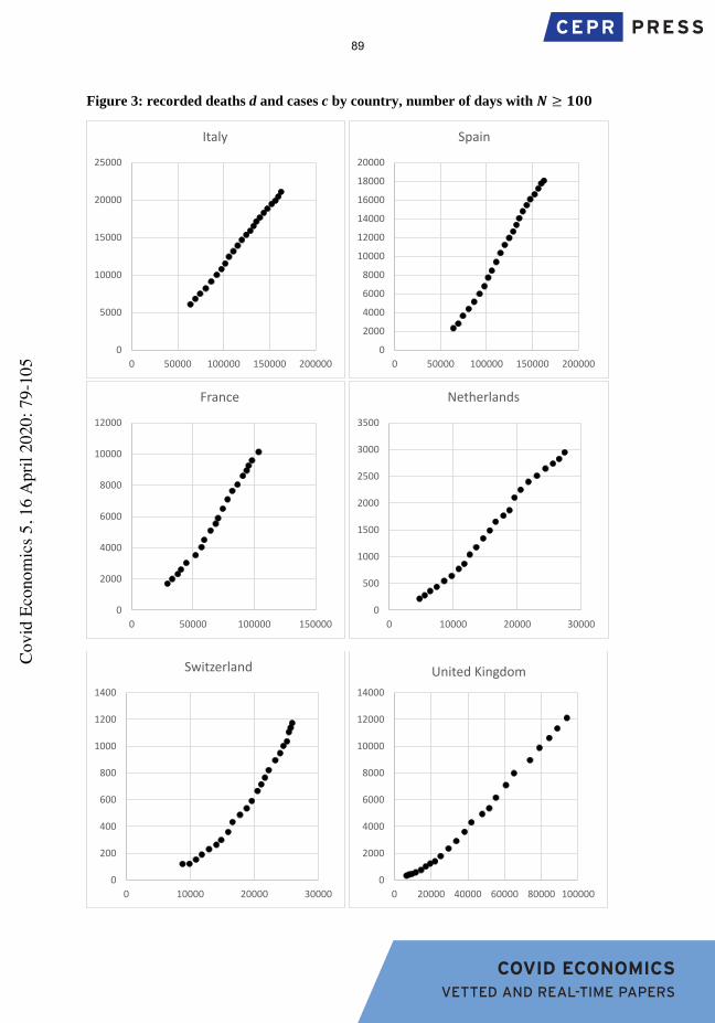
COVID ECONOMICS VETTED AND REAL-TIME PAPERS
Figure 3: recorded deaths d and cases c by country, number of days with 𝑵𝑵 ≥ 𝟏𝟏𝟏𝟏𝟏𝟏
0
5000
10000
15000
20000
25000
0 50000 100000 150000 200000
Italy
0
2000
4000
6000
8000
10000
12000
14000
16000
18000
20000
0 50000 100000 150000 200000
Spain
0
2000
4000
6000
8000
10000
12000
0 50000 100000 150000
France
0
500
1000
1500
2000
2500
3000
3500
0 10000 20000 30000
Netherlands
0
200
400
600
800
1000
1200
1400
0 10000 20000 30000
Switzerland
0
2000
4000
6000
8000
10000
12000
14000
0 20000 40000 60000 80000 100000
United Kingdom
89C
ovid
Eco
nom
ics 5
, 16
Apr
il 20
20: 7
9-10
5

COVID ECONOMICS VETTED AND REAL-TIME PAPERS
Figure 3 reveals what appears to be an emerging S-shaped relationship between cases 𝑐𝑐 on the x-axis and fatalities 𝑑𝑑 on the y-axis. Country effects are largely borne out by differences in levels, less so by the shape of the graph itself. In Germany where the approach to testing has been aggressive and where authorities doubled down on testing as the epidemic developed, the shape appears more irregular than elsewhere. This may be attributed to policy interventions, but more research is needed to identify possible causes.
To highlight the role of country specifics, the evidence is combined in Figure 4, now on a double logarithmic scale.
0
500
1000
1500
2000
2500
3000
3500
0 50000 100000 150000
Germany
0
50
100
150
200
250
300
350
400
450
0 5000 10000 15000
Austria
0
2000
4000
6000
8000
10000
12000
0 50000 100000 150000 200000 250000
State of N.Y.
0
2000
4000
6000
8000
10000
12000
14000
16000
0 100000 200000 300000 400000 500000
Rest of USA
90C
ovid
Eco
nom
ics 5
, 16
Apr
il 20
20: 7
9-10
5
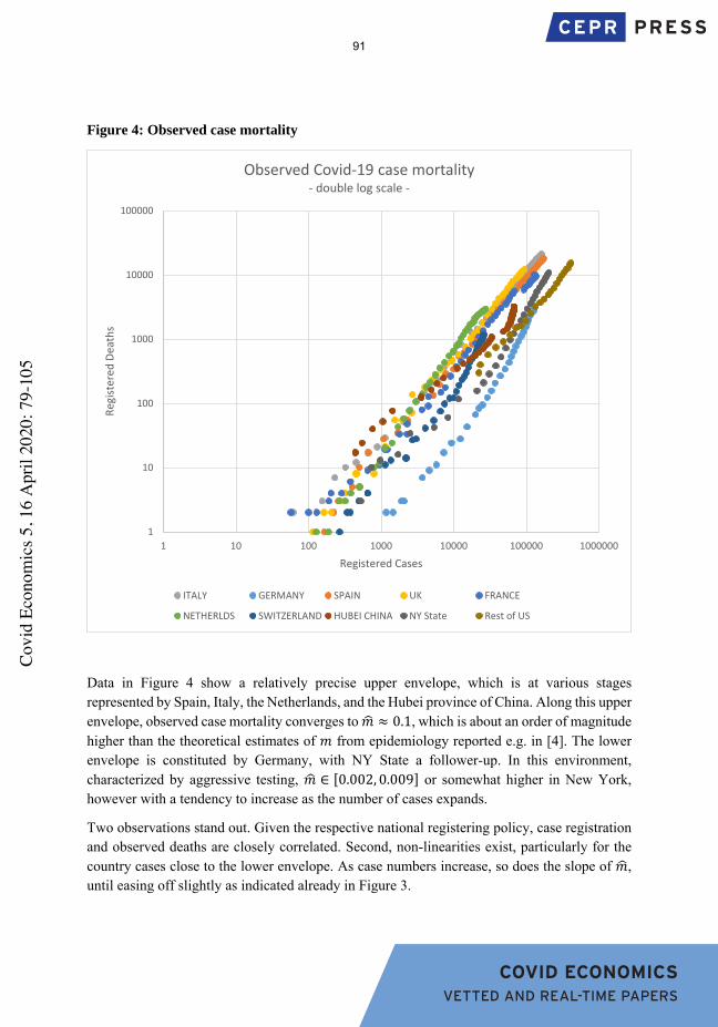
COVID ECONOMICS VETTED AND REAL-TIME PAPERS
Figure 4: Observed case mortality
Data in Figure 4 show a relatively precise upper envelope, which is at various stages represented by Spain, Italy, the Netherlands, and the Hubei province of China. Along this upper envelope, observed case mortality converges to 𝑚𝑚� ≈ 0.1, which is about an order of magnitude higher than the theoretical estimates of 𝑚𝑚 from epidemiology reported e.g. in [4]. The lower envelope is constituted by Germany, with NY State a follower-up. In this environment, characterized by aggressive testing, 𝑚𝑚� ∈ [0.002, 0.009] or somewhat higher in New York, however with a tendency to increase as the number of cases expands.
Two observations stand out. Given the respective national registering policy, case registration and observed deaths are closely correlated. Second, non-linearities exist, particularly for the country cases close to the lower envelope. As case numbers increase, so does the slope of 𝑚𝑚� , until easing off slightly as indicated already in Figure 3.
1
10
100
1000
10000
100000
1 10 100 1000 10000 100000 1000000
Regi
ster
ed D
eath
s
Registered Cases
Observed Covid-19 case mortality- double log scale -
ITALY GERMANY SPAIN UK FRANCE
NETHERLDS SWITZERLAND HUBEI CHINA NY State Rest of US
91C
ovid
Eco
nom
ics 5
, 16
Apr
il 20
20: 7
9-10
5

COVID ECONOMICS VETTED AND REAL-TIME PAPERS
Taken together, both figures confirm the evidence on strong country effects, although these do not appear to be linear or fixed. They also reveal an upper bound that is perhaps defined by overall Covid-19 mortality of hospital patients, and a lower bound that at times comes close to estimates of Covid-19 mortality among the general population.
V. Forecasting the end of the epidemic
Covid-19 related series are unreliable and short. Under normal circumstances this would warrant abstaining from forecasting exercises. Given current conditions, an exception to usual professional standards may be taken. Figures 6 provides ETS forecasts of the timing of Covid-19 for the counties in the sample, both for fatalities 𝑑𝑑 and total cases 𝑐𝑐. The nonlinearities in 𝑑𝑑/𝑐𝑐 suggest univariate rather than bivariate forecasts.
Absent errors in variables, predicted growth in registered cases should converge to zero 𝑠𝑠 calendar days before predicted fatality growth rates do, where 𝑠𝑠 is the average lag from recorded infection to death. Figure 6 presents country by country forecasts from the logarithmic differences in fatalities shown in Figure 1, as well as from the logarithmic differences in case numbers underlying Figures 3 and 4.i
Figure 6: ETS forecasts of the Covid-19 epidemic by country (log differences)
(a) Italy aa) deaths (s=0) ab) cases (s=0)
0
0.005
0.01
0.015
0.02
0.025
0.03
0.035
0.04
0.045
5-Ap
r
12-A
pr
19-A
pr
26-A
pr
3-M
ay
0
0.005
0.01
0.015
0.02
0.025
0.03
0.035
0.04
5-Ap
r
12-A
pr
19-A
pr
26-A
pr
3-M
ay
92C
ovid
Eco
nom
ics 5
, 16
Apr
il 20
20: 7
9-10
5

COVID ECONOMICS VETTED AND REAL-TIME PAPERS
(b) Spain
ba) deaths (s=0) bb) cases (s=0)
c) France
ca) deaths(s=3) cb) cases (s=0)
0
0.01
0.02
0.03
0.04
0.05
0.06
6-Ap
r
8-Ap
r
10-A
pr
12-A
pr
14-A
pr
16-A
pr
18-A
pr
20-A
pr
22-A
pr
24-A
pr
0
0.005
0.01
0.015
0.02
0.025
0.03
0.035
0.04
0.045
0.05
6-Ap
r8-
Apr
10-A
pr12
-Apr
14-A
pr16
-Apr
18-A
pr20
-Apr
22-A
pr24
-Apr
26-A
pr28
-Apr
0
0.02
0.04
0.06
0.08
0.1
0.12
0.14
0.16
6-Ap
r
8-Ap
r
10-A
pr
12-A
pr
14-A
pr
16-A
pr
18-A
pr
20-A
pr
22-A
pr
24-A
pr
26-A
pr
28-A
pr
0
0.01
0.02
0.03
0.04
0.05
0.06
6-Ap
r
8-Ap
r
10-A
pr
12-A
pr
14-A
pr
16-A
pr
18-A
pr
20-A
pr
22-A
pr
24-A
pr
26-A
pr
28-A
pr
Cov
id E
cono
mic
s 5, 1
6 A
pril
2020
: 79-
105
93

COVID ECONOMICS VETTED AND REAL-TIME PAPERS
d) Netherlands
da) deaths (s=0) db) cases (s=0)
e) New York State
ea) deaths (s=2) eb) cases (s=2)
0
0.02
0.04
0.06
0.08
0.1
0.12
0.14
6-Ap
r
8-Ap
r
10-A
pr
12-A
pr
14-A
pr
16-A
pr
18-A
pr
20-A
pr
22-A
pr
24-A
pr
26-A
pr
28-A
pr
0
0.01
0.02
0.03
0.04
0.05
0.06
0.07
6-Ap
r
8-Ap
r
10-A
pr
12-A
pr
14-A
pr
16-A
pr
18-A
pr
20-A
pr
22-A
pr
24-A
pr
26-A
pr
28-A
pr
0
0.02
0.04
0.06
0.08
0.1
0.12
0.14
0.16
0.18
6-Ap
r
8-Ap
r
10-A
pr
12-A
pr
14-A
pr
16-A
pr
18-A
pr
20-A
pr
22-A
pr
24-A
pr
26-A
pr
28-A
pr
0
0.02
0.04
0.06
0.08
0.1
0.12
0.14
0.16
0.18
6-Ap
r
8-Ap
r
10-A
pr
12-A
pr
14-A
pr
16-A
pr
18-A
pr
20-A
pr
22-A
pr
24-A
pr
26-A
pr
28-A
pr
Cov
id E
cono
mic
s 5, 1
6 A
pril
2020
: 79-
105
94

COVID ECONOMICS VETTED AND REAL-TIME PAPERS
f) United Kingdom
fa) deaths (s=0) fb) cases (s=0)
g) Switzerland
ga) deaths (s=0) gb) cases (s=0)
0
0.02
0.04
0.06
0.08
0.1
0.12
0.14
0.16
6-Ap
r
8-Ap
r
10-A
pr
12-A
pr
14-A
pr
16-A
pr
18-A
pr
20-A
pr
22-A
pr
24-A
pr
26-A
pr
28-A
pr
0
0.02
0.04
0.06
0.08
0.1
0.12
0.14
6-Ap
r
13-A
pr
20-A
pr
27-A
pr
4-M
ay
0
0.01
0.02
0.03
0.04
0.05
0.06
0.07
0.08
0.09
0.1
6-Ap
r
8-Ap
r
10-A
pr
12-A
pr
14-A
pr
16-A
pr
18-A
pr
20-A
pr
22-A
pr
24-A
pr
26-A
pr
28-A
pr
0
0.005
0.01
0.015
0.02
0.025
0.03
0.035
0.04
0.045
0.05
6-Ap
r8-
Apr
10-A
pr12
-Apr
14-A
pr16
-Apr
18-A
pr20
-Apr
22-A
pr24
-Apr
26-A
pr28
-Apr
Cov
id E
cono
mic
s 5, 1
6 A
pril
2020
: 79-
105
95

COVID ECONOMICS VETTED AND REAL-TIME PAPERS
h) Germany
ha) deaths (s=0) hb) cases (s=0)
i) Sweden
ia) deaths (s=0) ib) cases (s=0)
0
0.02
0.04
0.06
0.08
0.1
0.12
0.14
0.16
0.18
6-Ap
r
8-Ap
r
10-A
pr
12-A
pr
14-A
pr
16-A
pr
18-A
pr
20-A
pr
22-A
pr
24-A
pr
26-A
pr
28-A
pr
0
0.01
0.02
0.03
0.04
0.05
0.06
6-Ap
r8-
Apr
10-A
pr12
-Apr
14-A
pr16
-Apr
18-A
pr20
-Apr
22-A
pr24
-Apr
26-A
pr28
-Apr
30-A
pr
0
0.05
0.1
0.15
0.2
0.25
6-Ap
r
8-Ap
r
10-A
pr
12-A
pr
14-A
pr
16-A
pr
18-A
pr
20-A
pr
22-A
pr
24-A
pr
26-A
pr
28-A
pr
0
0.01
0.02
0.03
0.04
0.05
0.06
0.07
0.08
0.09
0.1
6-Ap
r
8-Ap
r
10-A
pr
12-A
pr
14-A
pr
16-A
pr
18-A
pr
20-A
pr
22-A
pr
24-A
pr
26-A
pr
28-A
pr
96C
ovid
Eco
nom
ics 5
, 16
Apr
il 20
20: 7
9-10
5

COVID ECONOMICS VETTED AND REAL-TIME PAPERS
j) Rest of the US
ja) deaths (s=0) jb) cases (s=0)
k) Austria
ka) deaths (s=0) kb) cases (s=0)
For all countries in Figure 6, the central forecast of at least one of the two indictors falls to zero within the coming weeks, which if it comes to pass means the end of the current epidemic wave is imminent. However, the precision of the forecasts varies strongly. Table 2 provides the projected end dates by country and indicator in approximate rank order.
0
0.02
0.04
0.06
0.08
0.1
0.12
0.14
0.16
0.18
0.2
6-Ap
r
8-Ap
r
10-A
pr
12-A
pr
14-A
pr
16-A
pr
18-A
pr
20-A
pr
22-A
pr
24-A
pr
26-A
pr
28-A
pr
0
0.02
0.04
0.06
0.08
0.1
0.12
6-Ap
r
8-Ap
r
10-A
pr
12-A
pr
14-A
pr
16-A
pr
18-A
pr
20-A
pr
22-A
pr
24-A
pr
26-A
pr
28-A
pr
0
0.02
0.04
0.06
0.08
0.1
0.12
0.14
6-Ap
r
8-Ap
r
10-A
pr
12-A
pr
14-A
pr
16-A
pr
18-A
pr
20-A
pr
22-A
pr
24-A
pr
26-A
pr
28-A
pr
0
0.005
0.01
0.015
0.02
0.025
0.03
6-Ap
r8-
Apr
10-A
pr12
-Apr
14-A
pr16
-Apr
18-A
pr20
-Apr
22-A
pr24
-Apr
26-A
pr28
-Apr
97C
ovid
Eco
nom
ics 5
, 16
Apr
il 20
20: 7
9-10
5
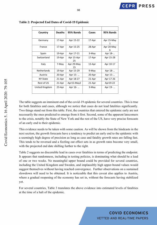
COVID ECONOMICS VETTED AND REAL-TIME PAPERS
Table 2: Projected End Dates of Covid-19 Epidemic
Country Deaths 95% Bands Cases 95% Bands
Germany 17-Apr Apr 15-22 17-Apr Apr 15-May 1
France 17-Apr Apr 15-25 28-Apr Apr 20-May 6
Spain 19-Apr Apr 17-21 3-May Apr 18-… Switzerland 19-Apr Apr 15-Apr
25 17-Apr Apr 15-28
Italy 7-May Apr 29-May 15
13-Apr Apr 10-17
Netherlands 19-Apr Apr 15-29 9-May Apr 18-… Austria 20-Apr Apr 15- … 20-Apr Apr 15-…
NY State 21-Apr Apr 18-27 21-Apr Apr 17-26 Rest of US 21-Apr Apr15-May2 21-Apr Apr19-22
United Kingdom 23-Apr Apr 16- … 3-May Apr 19- …
The table suggests an imminent end of the covid-19 epidemic for several countries. This is true for both fatalities and cases, although we notice that cases do not lead fatalities significantly. Two things stand out from this table. First, the countries that entered the epidemic early are not necessarily the ones predicted to emerge from it first. Second, some of the apparent latecomers to the crisis, notably the State of New York and the rest of the US, have very precise forecasts of an early end to their epidemic.
This evidence needs to be taken with some caution. As will be shown from the hindcasts in the next section, the growth forecasts have a tendency to predict an early end to the epidemic with a seemingly high degree of precision as long as case and fatality growth rates are falling fast. This tends to be reversed and a fizzling out effect sets in as growth rates become very small, with the projected end date shifting further to the right.
Table 2 suggests no discernible lead in cases over fatalities in terms of predicting the endpoint. It appears that randomness, including in testing policies, is dominating what should be a lead of one or two weeks. No meaningful upper bound could be provided for several countries, including the United Kingdom and Sweden, and implausibly high upper-bound values would suggest themselves without having reached convergence. Further observations on a sustained slowdown will need to be obtained. It is noticeable that this caveat also applies to Austria, where a gradual reopening of the economy has set in, without the forecasts having stabilized yet.
For several countries, Table 3 translates the above evidence into estimated levels of fatalities at the time of a halt of the epidemic.
98C
ovid
Eco
nom
ics 5
, 16
Apr
il 20
20: 7
9-10
5

COVID ECONOMICS VETTED AND REAL-TIME PAPERS
Table 3: Projected Maximum Fatalities by Country
Country Central Forecast
95% Upper Bound
95% Lower Bound
Spain 19239 20135 18673 France 16877 24233 16299 Italy 27263 31649 24046 Germany 3511 4565 3396 Netherlands 3255 4780 3070 NY State 14395 20008 12264 Switzerland 1291 1599 1211
Again, these projected numbers are contingent on the stability of the forecasts in Figure 6 above. Any shocks to fatality rates, reporting etc. will translate into revisions of these data. Yet they represent the information set at the time the forecast was taken, i.e. what can be projected with some degree of confidence as of that date. Experimenting with bivariate forecasts from fatalities and reported cases generally led to a loss in precision. This is in spite of the apparently tight relationship between both indicators at the national level suggested by Figure 4.
VI. Hindcasts: Forecasts from March 31 and later realisations To check the robustness of the forecasts, this section presents results from forecasting fatalities and case growth rates as of March 31, and compares the predictions with later outcomes. This procedure is sometimes called ‘hindcasting’, it allows a simple visual check of whether the forecasts at the time had sufficiently stabilized. Figure 7 has the results.
Figure 7: ‘Hindcasting’ Covid-19, 31 March to 14 April
Italy a) deaths b) cases
0
0.02
0.04
0.06
0.08
0.1
0.12
0.14
23-M
ar26
-Mar
29-M
ar1-
Apr
4-Ap
r7-
Apr
10-A
pr13
-Apr
16-A
pr19
-Apr
22-A
pr25
-Apr
28-A
pr
0
0.01
0.02
0.03
0.04
0.05
0.06
0.07
0.08
0.09
23-M
ar26
-Mar
29-M
ar1-
Apr
4-Ap
r7-
Apr
10-A
pr13
-Apr
16-A
pr19
-Apr
22-A
pr25
-Apr
28-A
pr
99C
ovid
Eco
nom
ics 5
, 16
Apr
il 20
20: 7
9-10
5
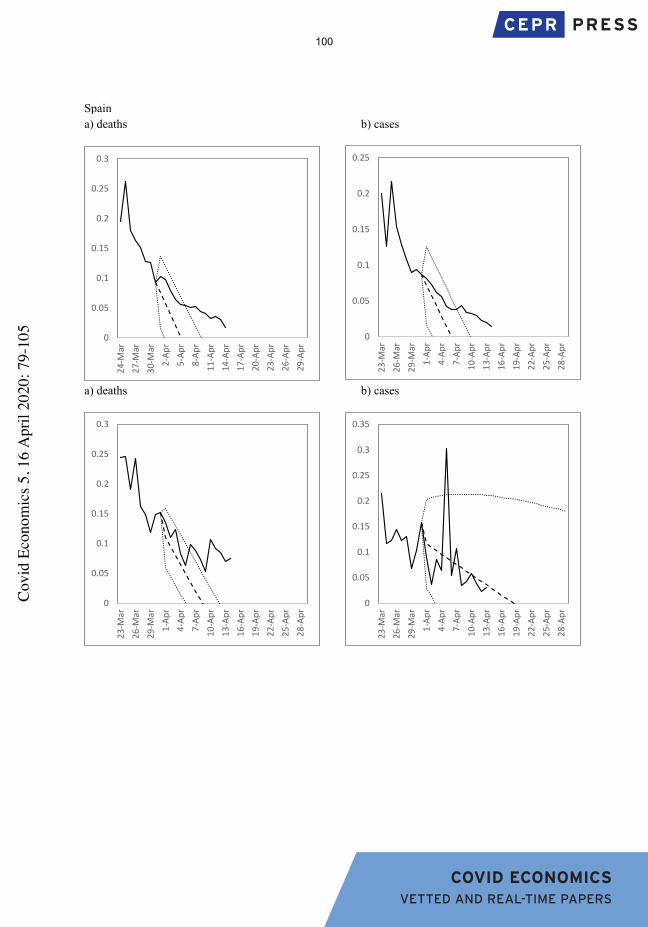
COVID ECONOMICS VETTED AND REAL-TIME PAPERS
Spain a) deaths b) cases
France a) deaths b) cases
0
0.05
0.1
0.15
0.2
0.25
0.3
24-M
ar27
-Mar
30-M
ar2-
Apr
5-Ap
r8-
Apr
11-A
pr14
-Apr
17-A
pr20
-Apr
23-A
pr26
-Apr
29-A
pr
0
0.05
0.1
0.15
0.2
0.25
0.3
23-M
ar26
-Mar
29-M
ar1-
Apr
4-Ap
r7-
Apr
10-A
pr13
-Apr
16-A
pr19
-Apr
22-A
pr25
-Apr
28-A
pr
0
0.05
0.1
0.15
0.2
0.25
23-M
ar26
-Mar
29-M
ar1-
Apr
4-Ap
r7-
Apr
10-A
pr13
-Apr
16-A
pr19
-Apr
22-A
pr25
-Apr
28-A
pr
0
0.05
0.1
0.15
0.2
0.25
0.3
0.35
23-M
ar26
-Mar
29-M
ar1-
Apr
4-Ap
r7-
Apr
10-A
pr13
-Apr
16-A
pr19
-Apr
22-A
pr25
-Apr
28-A
pr
100C
ovid
Eco
nom
ics 5
, 16
Apr
il 20
20: 7
9-10
5

COVID ECONOMICS VETTED AND REAL-TIME PAPERS
Netherlands a) deaths b) cases
Germany a) deaths b) cases
0
0.05
0.1
0.15
0.2
0.25
0.3
23-M
ar26
-Mar
29-M
ar1-
Apr
4-Ap
r7-
Apr
10-A
pr13
-Apr
16-A
pr19
-Apr
22-A
pr25
-Apr
28-A
pr
0
0.05
0.1
0.15
0.2
0.25
0.3
23-M
ar
30-M
ar
6-Ap
r
13-A
pr
20-A
pr
27-A
pr
0
0.02
0.04
0.06
0.08
0.1
0.12
0.14
0.16
0.18
23-M
ar26
-Mar
29-M
ar1-
Apr
4-Ap
r7-
Apr
10-A
pr13
-Apr
16-A
pr19
-Apr
22-A
pr25
-Apr
28-A
pr
0
0.02
0.04
0.06
0.08
0.1
0.12
0.14
0.16
0.18
23-M
ar
30-M
ar
6-Ap
r
13-A
pr
20-A
pr
27-A
pr
101C
ovid
Eco
nom
ics 5
, 16
Apr
il 20
20: 7
9-10
5

COVID ECONOMICS VETTED AND REAL-TIME PAPERS
United Kingdom a) deaths b) cases
Sweden a) deaths b) cases
0
0.05
0.1
0.15
0.2
0.25
23-M
ar26
-Mar
29-M
ar1-
Apr
4-Ap
r7-
Apr
10-A
pr13
-Apr
16-A
pr19
-Apr
22-A
pr25
-Apr
28-A
pr
0
0.05
0.1
0.15
0.2
0.25
0.3
0.35
0.4
0.45
0.5
23-M
ar26
-Mar
29-M
ar1-
Apr
4-Ap
r7-
Apr
10-A
pr13
-Apr
16-A
pr19
-Apr
22-A
pr25
-Apr
28-A
pr
0
0.1
0.2
0.3
0.4
0.5
0.6
23-M
ar
25-M
ar
27-M
ar
29-M
ar
31-M
ar
2-Ap
r
4-Ap
r
6-Ap
r
8-Ap
r
10-A
pr
12-A
pr
14-A
pr
0
0.05
0.1
0.15
0.2
0.25
0.3
23-M
ar26
-Mar
29-M
ar1-
Apr
4-Ap
r7-
Apr
10-A
pr13
-Apr
16-A
pr19
-Apr
22-A
pr25
-Apr
28-A
pr
102C
ovid
Eco
nom
ics 5
, 16
Apr
il 20
20: 7
9-10
5

COVID ECONOMICS VETTED AND REAL-TIME PAPERS
Austria a) deaths b) cases
State of New York a) deaths b) cases
0
0.05
0.1
0.15
0.2
0.25
0.3
0.35
23-M
ar
30-M
ar
6-Ap
r
13-A
pr
20-A
pr
27-A
pr
0
0.1
0.2
0.3
0.4
0.5
0.6
0.7
23-M
ar26
-Mar
29-M
ar1-
Apr
4-Ap
r7-
Apr
10-A
pr13
-Apr
16-A
pr19
-Apr
22-A
pr25
-Apr
28-A
pr
0
0.1
0.2
0.3
0.4
0.5
0.6
23-M
ar26
-Mar
29-M
ar1-
Apr
4-Ap
r7-
Apr
10-A
pr13
-Apr
16-A
pr19
-Apr
22-A
pr25
-Apr
28-A
pr
0
0.05
0.1
0.15
0.2
0.25
23-M
ar26
-Mar
29-M
ar1-
Apr
4-Ap
r7-
Apr
10-A
pr13
-Apr
16-A
pr19
-Apr
22-A
pr25
-Apr
28-A
pr
103C
ovid
Eco
nom
ics 5
, 16
Apr
il 20
20: 7
9-10
5

COVID ECONOMICS VETTED AND REAL-TIME PAPERS
Rest of the US a) deaths b) cases
The forecasts in Figure 7 bear out two things. First, in many cases the spread of the epidemic had slowed down sufficiently by the end of March to permit meaningful forecasts until very low rates of growth had been attained. During that period, forecasts from fatalities appear to perform better than forecasts from reported cases, as would be expected given the paramount reporting problems in the latter. Second, once daily growth rates of around 10% had been achieved, the process appears to fizzle out – a slowdown from the slowdown. In general, forecasting from the growth rates of fatalities appears to be warranted as a first check on the timing and orders of magnitude, requiring substantially less information than the attempt to estimate the SIR model itself.
VII. Conclusions
Univariate forecasts from the growth in fatalities and reported cases suggest that in some countries of Europe, the end of the epidemic is imminent. Growth in reported cases leads fatalities, however at lower lags than medical evidence would suggest. Nevertheless, predicted end dates for the epidemic are roughly consistent with each other. If confirmed, this would imply that in these countries, the peak burden on health services, especially on hospital ICUs, might be reached very soon. No such forecast can however be made at this time for countries where a slowdown in the rate of fatalities has not yet materialized or stabilized The evidence broadly suggests, however, that this is a matter of relatively short time. Utmost caution must be applied to these results, which are preliminary as they are based on very few observations. Better to err on the side of safety. Nevertheless, univariate forecasts especially from fatalities
0
0.05
0.1
0.15
0.2
0.25
0.3
0.35
0.4
23-M
ar26
-Mar
29-M
ar1-
Apr
4-Ap
r7-
Apr
10-A
pr13
-Apr
16-A
pr19
-Apr
22-A
pr25
-Apr
28-A
pr
0
0.05
0.1
0.15
0.2
0.25
0.3
24-M
ar27
-Mar
30-M
ar2-
Apr
5-Ap
r8-
Apr
11-A
pr14
-Apr
17-A
pr20
-Apr
23-A
pr26
-Apr
29-A
pr
104C
ovid
Eco
nom
ics 5
, 16
Apr
il 20
20: 7
9-10
5
COVID ECONOMICS VETTED AND REAL-TIME PAPERS
serve to give a meaningful idea of the timing and the magnitudes involved in the absence of reliable structural information on the parameters of the SIR model.
References
[1] Linton, Oliver, When will the Covid-19 pandemic peak? Mimeo, University of Cambridge, 2 April 2020.
[2] Fernandez-Villaverde, Jesus, and Chad Jones, Estimating and simulating a SIRD model of Covid-19, imeo, University of Pennsylvania, 13 April 2020.
[3] Homburg, Stefan, Effectiveness of Corona Lockdowns: Evidence for a Number of Countries, School of Economics and Uanagement, University of Hannover DP 671, 13 April 2020.
[4] Ferguson, Neil et al., Impact of non-pharmaceutical interventions (NPIs) to reduce COVID19 mortality and healthcare demand, Imperial College COVID-19 Response Team,[x] 16 March 2020, DOI
[5] ICNARC report on COVID-19 in critical care, 27 March 2020, doi
[6] Robert Koch Institut, Täglicher Lagebericht des RKI zur Coronavirus-Krankheit-2019 (COVID-19) , 03 March 2020.
[7] CSSE at Johns Hopkins University, https://github.com/CSSEGISandData
[8] Romer, Paul, Simulating Covid-19: Parts 1-3, 23-25 March, https://paulromer.net/archive/
[9] Eichenbaum, Martin, Sergio Rebelo, Mathias Trabandt, The Macroeconomics of Epidemics, NBER Working Paper 26882, April 2020.
[10] Donsimoni, Jean Roch , René Glawion, Bodo Plachter, Klaus Wälde, Projecting the Spread of
COVID19 for Germany, IZA WP 13094, March 2020. [11] Gros, Claudius, Roser Valenti, Kilian Valenti, Daniel Gros, Strategies for controlling the
medical and socio-economic costs of the Corona pandemic, https://arxiv.org/abs/2004.00493
[12] Stock, James, Dealing with data gaps, Covid Economics 3, CEPR, 14 April 2020.
[13] Data from https://www.gouvernement.fr/info-coronavirus/carte-et-donnees
i ETS forecasts of log fatality diffs, 95% confidence bands. ETS places successively smaller weights on more distant lags, roughly similar to the Litterman prior. Details and test statistics available upon request.
105C
ovid
Eco
nom
ics 5
, 16
Apr
il 20
20: 7
9-10
5

COVID ECONOMICS VETTED AND REAL-TIME PAPERS
Covid Economics Issue 5, 16 April 2020
Risk taking during a global crisis: Evidence from Wuhan1
Di Bu,2 Tobin Hanspal,3 Yin Lao4 and Yong Liu5
Date submitted: 5 April 2020; Date accepted: 7 April 2020
We conducted a repeated survey on risk taking behavior across a panel of subjects in Wuhan, China – ground zero of the Coronavirus pandemic – before and after the outbreak began. Our baseline survey was administered on October 16th, 2019 among graduate students in Wuhan prior to the COVID-19 outbreak. 47% of the students in our sample returned home to other provinces in China for semester break in early January before the province of Hubei and the city of Wuhan was locked down with strict quarantine orders on 23 January 2020. We administered a follow up survey to the same subjects, capturing their geolocation information on 28 February. We use variation in exposure across different Chinese cities and provinces to measure the impact of the Coronavirus pandemic on subjects’ willingness to take risk. We find that subjects’ allocations of wealth to hypothetical risky investments decrease monotonically based on the strength of their exposure to the pandemic. However, subjects uniformly report substantially lower general preferences for risk regardless of their exposure. Higher levels of exposure leads subjects to reduce beliefs in their own luck and sense of control and in turn, form more pessimistic beliefs on the economy and social conditions. We provide evidence that short-term changes in risk taking may stem more so from changes in beliefs and optimism than from general risk preferences. Our results suggest that more closely held formative experiences have large, negative, and acute effects on economic preferences during a crisis.
1 We are thankful to many for their suggestions, comments, and advice including Steffen Andersen, Claes Bäckman, Stefan Bogner, Martin Brown, Ray Fisman, Rawley Heimer, Matti Keloharju, Vesa Pursiainen, Michael Weber, and Christian Wagner. This project is supported by the Major Philosophy and Social Sciences Research Program of Hubei Province Higher Education Committee (Grant No.:19ZD016).
2 Senior Lecturer, Department of Applied Finance, Macquarie University.3 Assistant Professor of Finance, WU Vienna University of Economics and Business.4 Associate Professor, Department of Applied Finance, Macquarie University.5 Wuhan University of Science and Technology.
106C
ovid
Eco
nom
ics 5
, 16
Apr
il 20
20: 1
06-1
46
COVID ECONOMICS VETTED AND REAL-TIME PAPERS
1. Introduction
A number of studies have provided evidence that formative experiences stemming from large
shocks (e.g., financial crises, natural disasters, violence and trauma) may have long-term
effects on economic preferences and risk taking behavior (Malmendier and Nagel, 2011;
Kaustia and Knüpfer, 2008, 2012; Giannetti and Wang, 2016; Knüpfer, Rantapuska, and
Sarvimäki, 2017; Guiso, Sapienza, and Zingales, 2018; Andersen, Hanspal, and Nielsen, 2019;
and Brown, Cookson, Heimer, 2019). Most studies that investigate how these shocks affect
behavior use observational data on field outcomes and posit through which channels
behavior may have been affected. One missing aspect of these studies is how individual
preferences may acutely change, in the midst of the experience or crisis itself. To that end, we
know little about how the preferences and beliefs of individuals change during hard times.
Understanding how and why household risk taking and other preferences may
change during a crisis is crucial for determining appropriate policy responses, particularly
when the persistence of a downturn or crisis is unknown. If, for example, households’
tolerance for risk decreases through time-varying beliefs and expectations, it may imply that
observed changes in risk taking are temporary (e.g., financial market volatility and the
business cycle). At the same time, an expectations-driven shock to risk taking may impact
more strongly on consumption and consumer behavior. On the other hand, if changes in
observed risk taking come from a more general shift in preferences, policy responses may
need to be more structural in nature and may impact long term economic growth.
In this study, we examine how risk tolerance evolves from normal times, to the peak
of a worldwide health-crisis.1 We survey a large sample of subjects in Wuhan, China – ground
zero of the COVID-19 novel Coronavirus pandemic. Our first survey wave took place on
October 16th 2019, several weeks before initial reports of the virus in mainland China in
December 2019 (Holshue et al., 2020). By January 23rd, 2020 all incoming and outgoing public
transportation to and from the Hubei province (where Wuhan is the capital) was halted.
Gatherings and events inside Wuhan were banned, and quarantine and isolation were
established. By February 15th, 2020 Wuhan was in a state of complete and total quarantine
with more than 56,000 reported cases of COVID-19 infections and 1,600 deaths. On
February 28th 2020, we administered an online follow up survey to the same group of subjects
with an 88% retention rate (N = 225/257).
1 We plan to continue this study into the future, and further understand how risk taking and economic preferences continue to change or revert back to pre-crisis levels.
107C
ovid
Eco
nom
ics 5
, 16
Apr
il 20
20: 1
06-1
46

COVID ECONOMICS VETTED AND REAL-TIME PAPERS
Our main sample consists of graduate students from Wuhan University of Science
and Technology.2 Winter break for the semester started at WUST on January 11th 2020 and
most students from other provinces were able to return to their homes as planned for the
Chinese Lunar New Year celebrations. As the province of Hubei became quarantined and
effectively locked down shortly after, students from other provinces continued their study
programs via distance learning (alongside their Wuhan-based peers) and we administered
follow up online surveys on WeChat, capturing precise geolocation information from
subjects. This source of geographical variation across China allows us to measure the
intensity of exposure to the Coronavirus pandemic on our outcome measures of interest.
Wave one of our survey holds constant all subjects in the city of Wuhan, while in wave two,
47% of subjects (N = 106) are in provinces outside of Hubei, in parts of China with
substantially lower exposure to COVID-19. In fact, by the time our follow up study was
administered, February 28th, the province of Hubei had 66,300 infection cases, while all other
provinces across China had 12,600 in total. This variation allows us to explore if individuals
who are more closely impacted by the Coronavirus pandemic, as proxied by the province
and city of their quarantine location, differ in their preferences and beliefs as the crisis
evolves.
Our study examines if individuals’ tolerance for risk is affected due to their exposure
to the pandemic. We first document that subjects who become quarantined in Wuhan hold
subjective beliefs consistent with a higher level of exposure to the pandemic. These subjects
believe that they have a higher exposure risk to the Coronavirus than those elsewhere.
Subjects located in Wuhan during the quarantine state higher probabilities that they
themselves are likely to be infected, as well as higher exposure to infections and deaths within
their families and communities.3 Subjects across the province of Hubei also show higher
levels of fear in the pandemic in general.
We examine how varying exposure affects allocations to risk via a hypothetical
gamble elicited during the quarantine and peak of the Coronavirus pandemic in China during
the first week of March 2020. Subjects are asked to provide an allocation to a risky investment
(0-1000 RMB) invested with an equal probability of higher returns or a loss. Subjects
quarantined in Wuhan, with greater subjective (and arguably objective) exposure to the virus
2 As part of a separate project, we obtained additional survey data on perceptions of climate risk from both Wuhan and Guizhou, a province of China approximately 1,000 kilometers from Wuhan and one of the least affected areas from the Corona virus pandemic. This survey data was also collected in pre, and during-crisis waves similar to our main sample but is outside the scope of this particular paper. 3 We refer to these exposures to the virus as subjective perceptions about exposure because we can confirm that no individuals in our sample contracted the virus during our study period.
108C
ovid
Eco
nom
ics 5
, 16
Apr
il 20
20: 1
06-1
46

COVID ECONOMICS VETTED AND REAL-TIME PAPERS
allocate significantly less to the risky investment option relative to those in other cities within
the Hubei province (-67.0 RMB), and those in other provinces of China (-149.8 RMB). This
represents an economically significant difference given a mean investment of 287.6 RMB,
and constitutes a 45% smaller investment compared to subjects in other provinces.
We then attempt to disentangle the mechanism behind this observed difference in
risk taking by analyzing repeat-measures from our survey waves across a number of
outcomes. We find that on average all subjects surveyed first in Wuhan in October 2019, and
later at their place of quarantine show a large and significant decrease in general preferences
for risk. The decrease amounts to -0.63 on a 5 point scale and is highly significant at standard
levels (t-stat = -13.09). While the decrease in risk preferences for those in Wuhan, with higher
exposure to the pandemic, is slightly greater, the effect is economically and statistically small.
This suggests that the observed differences in risk taking from heterogeneous experiences
may not be entirely driven from the uniform decrease in general risk preferences.
We then examine several measures of optimism and beliefs in individuals’ own luck
and fortune prior to and during the Coronavirus pandemic and how they relate to risk taking.
Compared to other subjects, those in Wuhan, with higher exposure to the pandemic, show
a 10.2 percentage point decrease in Wuhan-based subjects in their belief about their own
personal luck. An index based on questions that ask about the percentage of investors which
would have better luck or higher returns in financial investments shows a similar pre-
pandemic value, while subjects quarantined in Wuhan submit a substantial increase in the
fraction of investors they believe are better than the subject him or herself (6.8 percentage
points). For subjects with higher exposure, measures about individuals’ sense of control are
similarly negatively affected. In general, we find that exposure strongly affects individuals’
optimism about their own outcomes.
The observed change in risk taking and in beliefs about self also affects broader
beliefs about the future economy and social conditions. We find that subjects with higher
exposure to the pandemic form more pessimistic beliefs on the economy in general, the stock
market, their own health, and on the environment, relative to subjects in further removed
provinces. A number of recent studies have focused on the importance of subjective beliefs
on economic outcomes (e.g., Kuhnen and Miu, 2017; Ameriks et al., 2018; Giglio et al., 2019;
Kuchler and Zafar, 2019; Das, Kuhnen, and Nagel, 2019; Andersen et al., 2020). Our findings
suggest that experiences may affect risk taking acutely through time-varying subjective
beliefs. What is not yet clear in our setting, is if the higher exposure led individuals to form
109C
ovid
Eco
nom
ics 5
, 16
Apr
il 20
20: 1
06-1
46

COVID ECONOMICS VETTED AND REAL-TIME PAPERS
more or less precise forecasts, although recent evidence suggests experience affects in the
opposite direction (Goldfayn-Frank and Wohlfart, 2019; Kuchler and Zafar, 2019).
Our paper contributes to the literature in economics and finance which examines
how events and experiences can shape behavior. In a seminal paper, Malmendier and Nagel
(2011) show that experiences with macroeconomic shocks affect financial risk taking well
into the future. A further literature has shown that personal experiences make individuals
refrain from opportunities to take risk (Knüpfer, Rantapuska, and Sarvimäki, 2017; Guiso,
Sapienza, and Zingales, 2018; Giannetti and Wang, 2016; Kaustia and Knüpfer, 2008, 2012;
Choi, Laibson, Madrian, and Metrick, 2009; Chiang, Hirshleifer, Qian, and Sherman, 2011;
Bucher-Koenen and Ziegelmeyer, 2014; Hoffmann and Post, 2017). Andersen, Hanspal, and
Nielsen (2019) highlight the importance of the degree to which individuals make experiences
and show that personal first-hand experiences can make individuals actively change their
attitudes toward risk. We contribute to this literature by providing evidence that closely
experienced shocks, in the midst of a crisis, can acutely affect risk taking at least partially
through a channel of beliefs and expectations. Relatedly, our findings contribute to a
literature on time-varying risk aversion (e.g., Campbell and Cochrane, 1999; Brandt and
Wang, 2003; Chetty and Szeidl, 2016; Brunnermeier and Nagel, 2008). We provide micro-
level evidence of changing attitudes towards risk. We document that general risk preferences
are uniformly negatively affected by the Coronavirus pandemic, while active risk taking
decisions may be more affected by individual level experiences through changing beliefs and
optimism.
We also contribute to a literature which uses survey or experimental data to measure
preferences and how heterogeneity in experiences affect these measures. For example, Callen
et al. (2013) find that risk aversion is exacerbated by violent wartime experiences, particularly
when these memories are made salient with priming. In contrast, Voors et al. (2012) and
Eckel et al. (2009) large shocks decrease risk aversion in their settings. Similarly, Fisman,
Jakiela, and Kariv (2015) find individuals exposed to the recession exhibit higher levels of
selfishness and in general that distributional preferences changed during the financial crisis
of 2007-09. We contribute to this literature by using repeated survey measures of economic
preferences and beliefs, and studying how risk taking is affected during times of crisis.
Finally, we contribute to a handful of recent studies which look at the effects of the
COVID-19 pandemic on households’ expectations.4 Binder (2020) surveys US households
4 Undoubtedly related to the Coronavirus pandemic is a number of studies which examine how beliefs about mortality affect economic decision making. The findings from this literature are mixed and use both individual surveys and life-cycle models (e.g., Hamermesh, 1985; Hurd and McGarry, 2002; Gan et al., 2015; Puri and
110C
ovid
Eco
nom
ics 5
, 16
Apr
il 20
20: 1
06-1
46
COVID ECONOMICS VETTED AND REAL-TIME PAPERS
relatively early during the course of the pandemic’s effects in the United States (March 3rd,
2020) and finds that subjects update their inflation and unemployment forecasts when
provided information about the Federal Reserve’s interest rates cuts. Fetzer et al., (2020) elicit
beliefs about mortality with two different information treatments and find that subjects
overestimate mortality and contagiousness of the virus. We contribute to this literature by
providing evidence of individuals’ updating of beliefs and preferences around the
Coronavirus pandemic, by using survey data on a repeat panel of subjects. Furthermore, our
subjects are under strict quarantine conditions and in the midst of the crisis.
Our study proceeds as follows: the second section provides additional background
on the Coronavirus setting in China. In Section 3 we detail our experimental setting,
discussing the baseline and follow-up survey along with information about participant
selection and the timing of events. In Section 4, we present our main findings along with
various other empirical results. We discuss the ramifications of our findings and conclude in
the final section.
2. Background
Our study focuses on how differences in exposure to the Coronavirus pandemic affect risk
taking and other economic outcomes. An implicit assumption about our empirical approach
and identification is that individuals located in different geolocations, i.e., the city of Wuhan,
the province of Hubei, and other provinces across China, differ in their exposure to the
Coronavirus pandemic. There are two, related, sources of variation by location which are
important to discuss. The first is spatial heterogeneity in rates of infection and death caused
by the COVID-19 Coronavirus. Figure 1 plots the cumulative infections (blue, left axis) and
deaths (red, right axis) in the Hubei province of China, where the city of Wuhan is located.
The dashed red and blue lines represent the cumulative sum of infections and deaths from
all other provinces in China and are plotted on the same axes. We note that other provinces
experienced significantly fewer infection cases and deaths compared to Hubei, and Wuhan,
the epicenter of the pandemic, over time. This variation implies that individuals in some
provinces of China will not have come into first-hand contact with the virus and are less
likely to know people who have been infected or died. On the other hand, individuals in the
city of Wuhan or the Hubei province are much more likely to experience the Coronavirus
either first-hand, or indirectly through family and friends.
Robinson, 2007; Cocco and Gomes, 2012; Elder, 2013; Post and Hanewald, 2013; Heimer, Myrseth, and Schoenle, 2019).
111C
ovid
Eco
nom
ics 5
, 16
Apr
il 20
20: 1
06-1
46

COVID ECONOMICS VETTED AND REAL-TIME PAPERS
Second, and related to the rates of infections and deaths, individuals across provinces
and cities in China experienced stark differences in regulations and quarantine conditions
during the Coronavirus pandemic. For example at the epicenter of the pandemic, in all cities
across the Hubei province, citizens were not permitted to go outside and leave their living
spaces under normal circumstances. Supermarkets, grocery stores, and pharmacies were not
open to serve individuals. Rather, the government organized special personnel to purchase
living materials for residents and distributed and delivered them throughout communities.
All public transportation was completely shut down. Furthermore, the local police patrolled
cities vigilantly and individuals found outside without permission were placed in government
assigned quarantine stations for 14 days.5
For individuals in other provinces across China, the quarantine conditions differed
substantially. In most areas, each household could assign a family member allowed to make
purchases for basic food and living materials every two days. Supermarkets, grocery stores,
and pharmacies remained open for individuals. Public transportation was only partially shut
down or disrupted for short periods of time in most cities. Finally, citizens were still
permitted to leave their communities for limited, necessary, activities. These differences in
quarantine conditions are directly related to the severity of the pandemic, however it is likely
that individuals experiencing the first-hand effects of the pandemic and the harshest
quarantine conditions will be significantly affected compared to those with lower exposure
to the virus itself as well as substantially more flexible living conditions.
3. Experimental design
a. Participant selection
In many universities across China students are grouped into cohorts in order to better
supervise and manage the large number of incoming students. The size of these cohorts
varies at different universities but are normally between 30 and 60 students. Once a cohort
is formed, the students generally remain within the same cohort for the entire study period
at their respective university. Cohorts differ from classes, and students from the same cohort
do not always attend the same lectures or study programs. Each cohort is managed by a
supervisor. This supervisor uses social networking apps and tools such as WeChat as a daily
communication and management platform for the students. Specifically, supervisors create
5 Firsthand accounts suggest that the quarantine measures in the city of Wuhan were a strong deterrent. Video clips circulating on social networking sites display police in Hubei arresting citizens and placing them into forced quarantine.
112C
ovid
Eco
nom
ics 5
, 16
Apr
il 20
20: 1
06-1
46

COVID ECONOMICS VETTED AND REAL-TIME PAPERS
a WeChat group for each class that they manage where students must join such that everyone
can be informed about announcements made by their supervisors. We use these cohorts and
WeChat groups to recruit and segment samples for participation in our study. To encourage
students to complete the survey, we offered students a small participation incentive (5 to 10
RMB).
b. Baseline surveys
From October 16, 2019 to October 18, 2019 we conducted a survey based experiment with
master students at Wuhan University of Science and Technology (WUST). The survey was
conducted primarily for a study on how beliefs about luck and superstition affect risk taking
and investment behavior.6 We administered the paper and pencil survey among 257 master’s
students in a classroom setting. Each postgraduate cohort at WUST typically comprises 30
to 40 postgraduate students. We randomly selected 8 postgraduate cohorts from a pool of
more than 90. We collaborated with the cohort supervisors who organized that their students
attend our survey sessions.
The survey consisted of several parts. First, students provided demographic
information such as age, gender, date of birth, and birth province. After this information
students were asked to answer a set of questions aimed to measure individual confidence (or
over-confidence). Specifically, subjects answered 10 trivia, fact-based questions and were
asked to provide a lower and upper bound for the 90 percent confidence interval of each
provided answer. Following these questions, subjects were asked to provide answers to five
standard and simple financial literacy questions on compounding interest, inflation, bond
and mortgage markets, and diversification.7
We then asked 13 questions on beliefs in good luck following Darke and Freedman
(1997). We then presented subjects a miscalibration exercise where we asked individuals to
provide probabilities over the last 12 months of Shenzhen Stock exchange index, the Chinese
top 300 stock index (CSI300), the S&P500 index, and GDP growth in China. We asked
individuals how confident they were of their answers. This was coupled with survey questions
asking how the subject would rank him or herself compared to others in their investment
performance. We then asked subjects about gambling and luck behavior with a 10 item
questionnaire (Wood and Clapham, 2005). Finally, we questioned subjects on their general
6 Work in progress by Bu et al., “Unlucky Beliefs: The Zodiac Birth Year Effect and Individual Investor Performance.” 7 Refer to Online Appendix A for an English translation of they survey questions.
113C
ovid
Eco
nom
ics 5
, 16
Apr
il 20
20: 1
06-1
46

COVID ECONOMICS VETTED AND REAL-TIME PAPERS
preferences for risk following (Dohmen et al., 2018). Photos of students taking the paper and
pencil survey are provided in Appendix Figure 1.8
From November 25, 2019 to December 3, 2019 we conducted a separate survey
among master students at WUST focused on beliefs and preferences related to climate
change. Similar to our main survey above, we administered this climate risk paper and pencil
survey among 12 randomly selected post graduate classes comprising 466 participants. The
sessions were administered with course counselors similar to described above. The focus of
this survey was on perceived climate change risk and pro-environmental behavior. This
sample is not included in our analysis and we plan to study this in a separate paper.
c. Follow up surveys
Shortly following the administration of our baseline survey, the city of Wuhan became the
epicenter for a worldwide health-crisis, the COVID-19 Coronavirus pandemic. Reports
suggest that the Coronavirus began in December 2019 in the Huanan seafood market in
downtown Wuhan (WHO, 2020). Winter break for the semester started at WUST on January
11th, 2020. Wuhan was locked down on January 23rd, 2020, and by then most students from
regions outside of Wuhan had left the city for holidays to celebrate China’s Lunar New Year.
From February 28, 2020 to March 3, 2020, we administered an online follow up
survey to the same subject pool as our first survey. The follow up was administered to 225
students from the original 257 student sample.9 All teaching activities were moved to online
distance learning initiatives. We were therefore able to create an online version of our initial
survey and students submitted their survey responses similar to their other course work.
Again, we collaborated with the managers of the student cohorts, this time to share the survey
link to the WeChat groups. The online survey tool allows us to capture precise information
about subjects’ location. We map the provided geolocation coordinates to cities and
provinces across China. A translated screenshot of the online survey is provided in Appendix
Figure 2.
8 In our experiment 130 students (51%) received a simple treatment while the other half acted as our control sample. The treated group of students were asked to read a short (approximately five-minute) excerpt from an article about the “Zodiac birth year” superstition, while the control group read a similar length article excerpt with content about the historical origin of Chinese New Year. This was for our original project on beliefs in luck and investment behavior. Controlling for, or studying sub-groups of within-sample have no economic or statistical effect on our results 9 At the same time, we randomly selected 25 new postgraduate cohorts from WUST for additional survey responses that we can follow into the future for related and follow up work. This sample is currently not part of our analysis. We also conducted follow up studies on our sample focused on beliefs and preferences related to climate change, however these subjects are not included in our main sample.
114C
ovid
Eco
nom
ics 5
, 16
Apr
il 20
20: 1
06-1
46

COVID ECONOMICS VETTED AND REAL-TIME PAPERS
In addition to the questions from our baseline survey, we also included questions on
generalized trust as found in the World Values Survey and Kosse et al. (2020) and Falk et al.
(2018). In addition to the miscalibration exercise from the first wave, we also asked
individuals to provide their probability assessment of future returns, i.e., their return
expectations, of the same indexes listed previously. We also included questions on general
uncertainty and subjects’ experiences with the Coronavirus.
Table 1 provides descriptive statistics on the subjects in our main sample. Panel B
shows the mean values of age, gender and financial literacy score for subjects from Wuhan
and those from other provinces in wave one of our survey. We note that the sample is highly
balanced along these variables.
4. Main results
a. Perceptions of exposure to the Coronavirus pandemic
The starting point of our study is to measure how individuals in our sample perceive their
exposure to COVID-19. In Figure 2, we plot the mean response to survey questions asking
subjects about exposure to infection cases. We compare the mean responses from students
who are quarantined in Wuhan with students who are quarantined in the province of Hubei,
outside of Wuhan, and with WUST students who returned to other provinces during
semester and are quarantined in other, less effected, provinces of China. We largely find that
students in Wuhan believe that they have a higher exposure to the Corona virus than students
located elsewhere. Figure 2 plots this result across panels for suspected cases in the
community where the subject is currently quarantined, confirmed cases in the community
where the subject is currently, confirmed cases among family and friends, and confirmed
deaths from Coronavirus in the community where the subject is currently. Table 2 presents
this results in a regression framework. We note that our main analyses uses OLS linear
regressions however our results are robust to nonlinear methods or ordered logit regressions
(as many of the survey questions are on ordinal scales).
The differences in subjective beliefs individuals have about their exposure to
Coronavirus are likely to be realistic. As noted, Figure 1 plots the cumulative infections (blue,
left axis) and deaths (red, right axis) in the Hubei province of China, where Wuhan is located.
The dashed red and blue lines represent the cumulative sum of infections and deaths from
all other provinces in China and are plotted on the same axes. The dashed gray line states the
timing of our follow up survey wave. We note that other provinces experienced a significantly
115C
ovid
Eco
nom
ics 5
, 16
Apr
il 20
20: 1
06-1
46

COVID ECONOMICS VETTED AND REAL-TIME PAPERS
fewer infection cases and deaths compared to Hubei, and Wuhan, the epicenter of the
pandemic, at the time of our follow up survey.
b. Fear of the Coronavirus pandemic
Given that subjects in our sample have varying levels of exposure to the pandemic, we expect
this to result in differences in perceived fear and risk of the virus itself. We test this in Table
3 and plot the results in Figure 3. Panel A displays the mean values of the question ‘do you
think you are likely to become infected with COVID-19?’ Responses are on a scale between
(1) and (5) for ‘very unlikely to ‘very likely.’ Panel B plots the mean values of a question
asking if the subject is afraid of the Coronavirus pandemic. Responses are on a scale between
(1) and (5) for ‘not afraid at all’ to ‘very afraid.’ We find that subjects located in Wuhan during
the quarantine state that they are more likely to be infected with COVID-19, and subjects in
the provinces of Hubei and Wuhan are equally more afraid of the virus in general compared
to those in other provinces.
c. Risk perceptions during the Coronavirus pandemic
Having established that individuals quarantined in Wuhan have higher exposure and more
fear of the pandemic, the natural next step is to examine how subjects perceive risk, and if
their tolerance to risk is affected due to varying exposure and experiences made during the
pandemic.
We first study how differences in exposure affects financial risk taking by eliciting
subjects’ allocation to a risky investment from a hypothetical gamble. This measure of
financial risk taking was elicited in our survey during the Coronavirus pandemic in March
2020. Subjects can chose an amount (0-1000 RMB) to be invested with 50% probability of
a higher return (3000 RMB if all invested) or 50% probability of a loss (0 RMB if all invested).
The alternative investment is a risk free payment (1000 RMB if all invested). We differentiate
between students who are quarantined in Wuhan, versus those who are quarantined at home
in Hubei, and those in different provinces in China. Panel A of Figure 4 shows that subjects
in Wuhan, with greater exposure to the pandemic, allocate significantly less to the risky
gamble. The mean (median) investment across the entire sample is 287.6 (200) RMB. Panel
A of Table 4 highlights cross-sectional differences in exposure in the amount invested. The
variables of interest are indicators for where the subjects are located during March 2020. In
Columns 1 and 3, Hubei is defined as individuals in Hubei and Wuhan (anyone in the
116C
ovid
Eco
nom
ics 5
, 16
Apr
il 20
20: 1
06-1
46

COVID ECONOMICS VETTED AND REAL-TIME PAPERS
province), while in Columns 2, 4, 5, 6 we code the variable as 1 for individuals in Hubei, but
outside of Wuhan. Therefore, Column 1 provides an estimate of the difference in the risky
allocation of subjects in Wuhan relative to those in Hubei. In Columns 2, 4, 5 and 6, we then
quantify the difference between individuals in Wuhan and those in other provinces.10 In
Columns 3-4 we add control variables (gender, age, financial literacy score), and in Column
5 (6) we analyze sub-samples of men (women). We note across the table, subjects in Wuhan
allocate a significant less wealth to the risky financial lottery option. The effect is
economically and statistically significant and represents a 45% decrease in investment relative
to subjects in other provinces. We note that women with greater exposure to the pandemic
in our sample allocate even less to the risky investment compared to those with further
removed experiences. The heterogeneity in risk taking by gender is in line with previous
findings (Croson and Gneezy, 2009; Charness and Gneezy, 2012; Andersen et al., 2020), and
complements recent findings about how gender norms and experiences affect economic
outcomes and forecasts (D’Acunto et al., 2019; D’Acunto, Malmendier and Weber, 2020).
One question which arises is through which mechanism do contemporaneous
experiences affect risk taking? A body of work has documented heterogeneity over the life-
cycle and stability in general preferences (Dohmen et al., 2017; Falk et al., 2018). Recent
literature has focused on potential explanations for changing observed measures of risk
taking. Time-varying risk aversion may be a function of changing emotions, e.g., fear
(Loewenstein et al., 2001; Goetzmann, Kim, and Shiller, 2016; Guiso, Sapienza, and Zingales,
2019), and potentially time-varying beliefs or expectations. The latter has been discussed
broadly, (e.g. Malmendier and Nagel, 2011), however are difficult to pinpoint empirically.
We therefore first investigate how general preferences for risk evolved through the
Coronavirus pandemic. In Panels B and C of Figure 4, we plot the risk preference index
score from two established survey questions on general attitudes to risk. The first question
is a direct translation of the general risk preference question validated by Falk et al., (2016,
2018), ‘In general, how willing are you to take risks?’ The second question is ‘Will you take
more risk this year compared to last year.’ Both questions ask subjects to respond on a scale
of 1 to 5. We combine the answers of both questions into an equally weighted scale which
ranges from 1 (low willingness to take risk) to 5 (high willingness to take risk). These risk
questions are elicited in October 2019, and repeated in March 2020 amongst our panel of
10 In Appendix Table 1, we present all regressions using our Column 1-definition of Hubei and note the relationship is statistically and economically significant. Across columns we also vary the definition of the risky allocation by dropping outliers and removing potential misinterpreted responses. The table shows that excluding these observations, and alternative specifications, have no quantitative effect on our results.
117C
ovid
Eco
nom
ics 5
, 16
Apr
il 20
20: 1
06-1
46

COVID ECONOMICS VETTED AND REAL-TIME PAPERS
subjects. Panel B shows that the total sample of subjects elicited first in Wuhan and later at
the place of the quarantine show a large and significant decrease in risk appetite (an increase
to risk aversion). The decrease amounts to -0.64 on the 5 point scale and is significant at
standard levels (t-stat = -13.09). Given a mean value in wave one of 2.54, this constitutes a
substantial 25.2% decrease. When we consider if subjects in Wuhan compared to those in
other regions further removed from the pandemic, reduce preferences for risk as measured
by our general risk index, we find that all groups seem to decrease equally in their preferences
of risk (Panel C). Our generalized measures of risk do not seem to vary more for subjects
with higher exposure to the pandemic compared to those outside of the most affected
province. This suggests that the observed differences in risk taking, as measured by allocation
decisions, may not be driven solely by changes in general risk preferences. In Panel B of
Table 4 we present these results in a traditional regression framework. Hubei subjects is an
indictor variable which takes the value of one if subjects are quarantined in the Hubei
province, while Wuhan subjects takes the value of one if subjects are quarantined within the
city of Wuhan. Wave two indicates the timing of March 2020 from our second survey wave
and the variables of interest are the interaction of the two location variables with the time
trend. In Columns 3 and 7 the interaction term of Wuhan and Wave two is relative to Hubei
subjects, while in Columns 4 and 8 it is relative to other provinces. We note that while the
coefficients on our variable of interest, Wuhan subjects x wave two, is negative it is not
statistically different from zero. As mentioned, the time trend indicator, wave two, is highly
negative and statistically significant across specifications.
Our results show a large increase in risk aversion from before the Coronavirus
pandemic to its peak in Wuhan. It is plausible that this effect is partially driven by an increase
in fear as attributed to risk taking following the financial crisis of 2007-2009 (Guiso, Sapienza,
and Zingales, 2018). However, as shown in Figures 2 and 3, higher fear and second-hand
experiences (exposure to COVID-19 via family and community) are concentrated among
individuals with higher levels of exposure.11 Two additional, and related channels which we
wish to examine are how optimism, beliefs about luck and fortune, and beliefs about the
economy can influence risk taking. We explore these two channels in the following sections.
11 We note that when we analyze changes in general risk taking by geolocation and second-hand experiences we find complementary evidence that all subjects reduce risk taking, regardless if they have experienced deaths or illnesses within their family and community, within Wuhan as well as in other provinces, however as the sample sizes are smaller the standard errors become large.
118C
ovid
Eco
nom
ics 5
, 16
Apr
il 20
20: 1
06-1
46

COVID ECONOMICS VETTED AND REAL-TIME PAPERS
d. Optimism and beliefs about luck and fortune
As our initial study was formulated to study optimism, beliefs in individuals’ own luck, and
investment decisions, we elicited several measures of these behavioral traits prior to and
during the Coronavirus pandemic. In Table 5 we explore how these measures evolved over
time, and how experience with the pandemic may affect them. Figure 5 presents the results
visually. In Panel A we plot the mean values of an index of optimism created based on
individuals’ belief in good luck from Darke and Freedman (1997),12 which ranges from 0 (low
belief in their own personal luck) to 1 (high belief in their own personal luck). The score was
elicited in October 2019, and repeated in March 2020. As previously, we plot the values for
both periods based on subjects’ exposure, proxied by location in March. We examine the
differences quantitatively in Table 5. As previous, the variables of interest are Hubei subjects,
an indictor variable which takes the value of one if subjects are quarantined in the Hubei
province, Wuhan subjects, which takes the value of one if subjects are quarantined in the city
of Wuhan, and the interaction of the two location variables with the time trend. Across
panels, in Column 3 the interaction term of Wuhan and wave two is relative to Hubei subjects,
while in Column 4 it is relative to other provinces. In Column 2, we note a large decrease for
subjects in Wuhan in their beliefs about how lucky they are personally (7.2 percentage points,
p-value 0.003), while prior to the pandemic their belief in luck was statistically equivalent to
subjects from other provinces. Note that this effect in Column 2 relates the difference to the
average individual across other provinces as well as Hubei. Column 3 relates the difference
to other subjects in Hubei outside of the city of Wuhan. The coefficient here is negative as
expected, but not significant. In Column 4 the coefficient relates the difference in Wuhan to
those in other provinces and outside of Hubei. The effect is -10.2 percentage points with a
p-value < 0.0001.
Panel B similarly plots an index based on questions that ask about the percentage of
investors who would have better luck or higher returns in financial investments. Again, we
note a similar pre-pandemic value for all subjects, for those quarantined in Wuhan we
observe a substantial increase from pre- to the midst of the pandemic, in the fraction of
investors better than the subject (6.8 percentage points, p-value < 0.0001).
Finally, in Panel C we plot the mean value of an index on beliefs about subjects’
control over their own outcomes and luck. The survey questions are based on the Drake
12 The index is created based on statements that subjects agree or disagree with such as ‘I consider myself to be a lucky person;’ ‘I believe in luck;’ and ‘I often feel like it’s my lucky day.’ Further information about the survey can be found in Online Appendix A.
119C
ovid
Eco
nom
ics 5
, 16
Apr
il 20
20: 1
06-1
46

COVID ECONOMICS VETTED AND REAL-TIME PAPERS
Beliefs about Chance (DRC) Inventory (Wood and Clapham, 2005) and contain a battery of
statements such as ‘If I concentrate hard enough I might be able to influence whether I win
when I play (game),’ and ‘If I am well prepared, I have very large likelihood to win a gamble.’
We note that subjects from Wuhan show lower beliefs in their individual sense of control as
measured by the DRC survey statements from pre-pandemic to its peak, relative to subjects
in other provinces. The economic magnitude of the mean effect is significant, -6.9 percentage
points, and is highly statistically significant, p-value = 0.003.
In general, our findings suggest that higher exposure to the Coronavirus pandemic,
and therefore more direct and acute experiences, have a strong negative effect on individuals’
beliefs, optimism, and sense of individual control. We argue that these beliefs are an
important component of risk taking.13 In the following section we examine how exposure to
the pandemic may affect broader beliefs about future economic activity and social
conditions.
e. Beliefs and expectations on economic indicators
Our findings thus far suggest that experiences may affect risk taking acutely through
pessimistic subjective beliefs. A number of recent studies have focused on the importance
of subjective beliefs on economic outcomes (Kuhnen and Miu, 2017; Ameriks et al., 2018;
Giglio et al., 2019; Kuchler and Zafar, 2019; Das, Kuhnen, and Nagel, 2019; Andersen et al.,
2020). In Table 6, we study how subjects in our setting vary in their future expectations on
economic indicators based on their exposure to the Coronavirus pandemic.
We study expectations in two ways: first we measure scale-based survey questions on
future economic outcomes, i.e., ‘compared to last year, China’s economy (your health;
China’s natural environment) will become better in the next 12 months.’ The scale ranges
from (1) to (5) for ‘strongly disagree’ to ‘strongly agree.’ Secondly we ask subjects to assign
probabilities to market returns from 6 scenarios and form a probability distribution. We
create a measure of expected returns using the midpoints of these probability bins for the
Shanghai Stock Exchange index (SSE). All measures were elicited in our March 2020 survey
wave.
13 In Appendix Table 2 we examine to what extent changes in general risk taking and changes in beliefs explain lower risk allocations. Across the table the coefficient on decreases in optimism (and reduced general risk taking) largely correlate with lower risk allocations, however the standard errors are large and the coefficients are not precisely estimated. We do note that the coefficients on our exposure measures, subjects from Hubei and Wuhan, remain economically and statistically significant and absorb the variation from the more pessimistic belief variables confirming that those who reduce their optimism are indeed those with higher exposure.
120C
ovid
Eco
nom
ics 5
, 16
Apr
il 20
20: 1
06-1
46

COVID ECONOMICS VETTED AND REAL-TIME PAPERS
In Figure 7 we plot the mean values of these two types of expectation measures for
subjects quarantined in Wuhan, subjects in Hubei outside of the city of Wuhan, and for
subjects in other provinces of China. We note that subjects currently in Wuhan and therefore
arguably more closely experiencing the Coronavirus pandemic largely form more pessimistic
beliefs in the general economy, social conditions, and financial market indices, relative to
subjects in provinces further removed from the pandemic. Table 7 presents these results. As
these expectations are forward looking, we cannot ascertain if individuals with more acute
experiences provide more accurate responses, perhaps because they have more local and
relevant information, or if they are more likely to provide biased forecasts. In the first wave
of our survey we elicited miscalibration estimates of financial indices rather than forecasts
and found that individuals from different geolocations (prior to their exposure and
experience to the pandemic) did not differ statistically in their responses. Recent evidence
suggests experience may cause subjects to provide more imprecise forecasts (Goldfayn-Frank
and Wohlfart, 2019; Kuchler and Zafar, 2019). However, it is a research area which is
understudied and we hope to revisit this question in future survey waves. In general, our
results show that subjects with higher exposure to the pandemic form more pessimistic
beliefs on the economy, the stock market, their own health, and on the environment, relative
to subjects in further removed provinces.
5. Conclusion
In this paper, we study how risk taking and economic preferences evolve from normal times
to the peak of a worldwide health-crisis. We use repeated survey data from a panel of subjects
based in Wuhan, China. Our identification strategy exploits the fact that winter break for the
semester started on January 11th 2020 and students from other provinces were able to return
to their homes as planned for the Chinese Lunar New Year celebrations, providing quasi-
random variation in the exposure to the pandemic and quarantine conditions individuals
experience across China.
We find that subjects in Wuhan, with objectively higher exposure to the Coronavirus
pandemic, also believe that they have a higher exposure risk to the virus than those elsewhere.
They state higher probabilities that they are likely to be infected, and show higher levels of
fear in the pandemic in general. We then show that subjects more closely experiencing the
pandemic in Wuhan, reduce risk taking in an investment allocation task. At the same time,
experience does not differentially affect general preferences for risk – instead, on average, all
subjects surveyed first in Wuhan and later at their place of quarantine show a large and
121C
ovid
Eco
nom
ics 5
, 16
Apr
il 20
20: 1
06-1
46

COVID ECONOMICS VETTED AND REAL-TIME PAPERS
significant decrease in general risk appetite. We argue that this can be partially explained by
changes in optimism and beliefs about their own luck and sense of control. Furthermore,
higher exposure leads individuals to form more pessimistic beliefs on the economy, their
health, and the environment in general.
Our results present an important contribution to a large literature on risk taking
behavior after large shocks and formative experiences. While we provide confirmatory
evidence that risk taking behavior is indeed an artifact of experiences, we also show that
changes in risk taking seem to be more linked to time-varying beliefs and optimism than
general preferences for risk. In general our results help explain why individual level
experiences have a more pronounced effect on behavior than further removed experiences.
At the same time, our findings provide important supporting evidence for policy decision
making. If observed risk taking of households changes via time-varying beliefs and
expectations, the effects may only be temporary. On the other hand, changes in household
risk taking from more of a general shift in preferences may require policy that are larger, and
more structural, and may reflect a larger impact on long term economic growth.
Our work is an early study on the large consequences we expect to occur from the
global Coronavirus pandemic. Future work in our field and within our own research agenda
will study how these beliefs and preferences further evolve over time, link these measures to
field behavior, and exploit further heterogeneity in personal experiences.
122C
ovid
Eco
nom
ics 5
, 16
Apr
il 20
20: 1
06-1
46

COVID ECONOMICS VETTED AND REAL-TIME PAPERS
References:
Andersen, Steffen, Tobin Hanspal, and Kasper Meisner Nielsen. "Once bitten, twice shy:
The power of personal experiences in risk taking." Journal of Financial Economics 132.3 (2019): 97-117.
Andersen, S., Hanspal, T., Martinez-Correa, J. and Nielsen, K.M., 2020. Beliefs and Behavioral Biases. Working Paper.
Ameriks, J., G. Kézdi, M. Lee, and M.D. Shapiro. 2018. Heterogeneity in expectations, risk tolerance, and household stock shares: The attenuation puzzle. NBER Working Paper, 25269
Binder, C., 2020. Coronavirus Fears and Macroeconomic Expectations. Available at SSRN 3550858.
Bucher-Koenen, T., Ziegelmeyer, M., 2014. Once burned, twice shy? Financial literacy and wealth losses during the financial crisis. Review of Finance 18 (6), 2215-2246.
Brandt, M.W. and Wang, K.Q., 2003. Time-varying risk aversion and unexpected inflation. Journal of Monetary Economics, 50(7), pp.1457-1498.
Brown, J.R., Cookson, J.A. and Heimer, R.Z., 2019. Growing up without finance. Journal of Financial Economics, 134(3), pp.591-616.
Brunnermeier, M.K. and Nagel, S., 2008. Do wealth fluctuations generate time-varying risk aversion? Micro-evidence on individuals. American Economic Review, 98(3), pp.713-36.
Campbell, J.Y. and Cochrane, J.H., 1999. By force of habit: A consumption-based explanation of aggregate stock market behavior. Journal of Political Economy, 107(2), pp.205-251.
Chetty, R. and Szeidl, A., 2016. Consumption commitments and habit formation. Econometrica, 84(2), pp.855-890.
Choi, J. J., Laibson, D., Madrian, B. C., Metrick, A., 2009. Reinforcement learning and savings behavior. Journal of Finance 64 (6), 2515-2534.
Cocco, J.F. and Gomes, F.J., 2012. Longevity risk, retirement savings, and financial innovation. Journal of Financial Economics, 103(3), pp.507-529.
D’Acunto, F., Malmendier, U., Ospina, J. and Weber, M., 2019. Exposure to daily price changes and inflation expectations (No. w26237). National Bureau of Economic Research.
D’Acunto, F., Malmendier, U. and Weber, M., 2020. Gender Roles and the Gender Expectations Gap (No. w26837). National Bureau of Economic Research.
Darke, P.R. and Freedman, J.L., 1997. The belief in good luck scale. Journal of research in personality, 31(4), pp.486-511.
Das, S., C.M. Kuhnen, and S. Nagel. 2019. Socioeconomic status and macroeconomic expectations. The Review of Financial Studies 32 (3), 1148-1187.
Dohmen, T., Falk, A., Golsteyn, B.H., Huffman, D. and Sunde, U., 2017. Risk attitudes across the life course. The Economic Journal.
Elder, T.E., 2013. The predictive validity of subjective mortality expectations: Evidence from the health and retirement study. Demography, 50(2), pp.569-589.
Falk, A., Becker, A., Dohmen, T.J., Huffman, D. and Sunde, U., 2016. The preference survey module: A validated instrument for measuring risk, time, and social preferences. Working Paper
Falk, A., Becker, A., Dohmen, T., Enke, B., Huffman, D. and Sunde, U., 2018. Global evidence on economic preferences. The Quarterly Journal of Economics, 133(4), pp.1645-1692.
Fetzer, T., Hensel, L., Hermle, J. and Roth, C., 2020. Perceptions of Coronavirus Mortality and Contagiousness Weaken Economic Sentiment. arXiv preprint arXiv:2003.03848.
123C
ovid
Eco
nom
ics 5
, 16
Apr
il 20
20: 1
06-1
46

COVID ECONOMICS VETTED AND REAL-TIME PAPERS
Gan, L., Gong, G., Hurd, M. and McFadden, D., 2015. Subjective mortality risk and bequests. Journal of Econometrics, 188(2), pp.514-525.
Giannetti, M., Wang, T. Y., 2016. Corporate scandals and household stock market participation. Journal of Finance 71 (6), 2591-2636.
Giglio, S., M. Maggiori, J. Stroebel, and S. Utkus. 2019. Five facts about beliefs and portfolios. NBER Working Paper, 25744.
Goetzmann, W.N., Kim, D. and Shiller, R.J., 2016. Crash beliefs from investor surveys (No. w22143). National Bureau of Economic Research.
Goldfayn-Frank, O. and Wohlfart, J., 2019. Expectation formation in a new environment: Evidence from the German reunification. Journal of Monetary Economics.
Guiso, L., Sapienza, P., Zingales, L., 2008. Trusting the stock market. Journal of Finance 63 (6), 2557-2600.
Guiso, L., Sapienza, P., Zingales, L., 2018. Time-varying risk aversion. Journal of Financial Economics 128 (3), 403-421.
Hamermesh, D.S., 1985. Expectations, life expectancy, and economic behavior. The Quarterly Journal of Economics, 100(2), pp.389-408.
Heimer, R.Z., Myrseth, K.O.R. and Schoenle, R.S., 2019. YOLO: Mortality beliefs and household finance puzzles. The Journal of Finance, 74(6), pp.2957-2996
Hurd, M.D. and McGarry, K., 2002. The predictive validity of subjective probabilities of survival. The Economic Journal, 112(482), pp.966-985.
Holshue, M.L., DeBolt, C., Lindquist, S., Lofy, K.H., Wiesman, J., Bruce, H., Spitters, C., Ericson, K., Wilkerson, S., Tural, A. and Diaz, G., 2020. First case of 2019 novel coronavirus in the United States. New England Journal of Medicine.
Hoffmann, A., Post, T., 2017. How return and risk experiences shape investor beliefs and preferences. Accounting and Finance 57 (3), 759-788.
Kuchler, T., and B. Zafar. 2019. Personal experiences and expectations about aggregate outcomes. The Journal of Finance 74 (5), 2491-2542.
Kaustia, M., Knüpfer, S., 2008. Do investors overweight personal experience? Evidence from IPO subscriptions. Journal of Finance 63 (6), 2679-2702.
Knüpfer, S., Rantapuska, E. H., Sarvimäki, M., 2017. Formative experiences and portfolio choice: evidence from the Finnish Great Depression. Journal of Finance 72 (1), 133-166.
Kosse, F., Deckers, T., Pinger, P., Schildberg-Hörisch, H. and Falk, A., 2020. The formation of prosociality: causal evidence on the role of social environment. Journal of Political Economy, 128(2), pp.000-000.
Kuhnen, C. M. 2015. Asymmetric learning from financial information. The Journal of Finance 70(5), 2029–2062.
Kuhnen, C. M., and A.C. Miu. 2017. Socioeconomic status and learning from financial information. Journal of Financial Economics 124(2), 349–372.
Kuhnen, C.M., Sarah Rudorf, and Bernd Weber. 2017. The effect of prior choices on expectations and subsequent portfolio decisions. NBER Working Paper, 23438.
Loewenstein, G.F., Weber, E.U., Hsee, C.K. and Welch, N., 2001. Risk as feelings. Psychological bulletin, 127(2), p.267.
Malmendier, U., Nagel, S., 2011. Depression babies: do macroeconomic experiences affect risk taking? Quarterly Journal of Economics 126 (1), 373-416.
Post, T. and Hanewald, K., 2013. Longevity risk, subjective survival expectations, and individual saving behavior. Journal of Economic Behavior & Organization, 86, pp.200-220.
Puri, M. and Robinson, D.T., 2007. Optimism and economic choice. Journal of Financial Economics, 86(1), pp.71-99.
“Novel Coronavirus – China.” World Health Organization, World Health Organization, 13
124C
ovid
Eco
nom
ics 5
, 16
Apr
il 20
20: 1
06-1
46

COVID ECONOMICS VETTED AND REAL-TIME PAPERS
Jan. 2020, www.who.int/csr/don/12-january-2020-novel-coronavirus-china/en/. Wood, W.S. and Clapham, M.M., 2005. Development of the drake beliefs about chance
inventory. Journal of Gambling Studies, 21(4), pp.411-430.
125C
ovid
Eco
nom
ics 5
, 16
Apr
il 20
20: 1
06-1
46

COVID ECONOMICS VETTED AND REAL-TIME PAPERS
Figure 1: Coronavirus infection cases and deaths in the Hubei province and across China
In the following figure we plot the cumulative infections (blue, left axis) and deaths (red, right axis) in the Hubei province of China, where Wuhan is located. The dashed red and blue lines represent the cumulative sum of infections and deaths from all other provinces in China and are plotted on the same axes. The dashed gray line states the timing of our follow up survey wave.
126C
ovid
Eco
nom
ics 5
, 16
Apr
il 20
20: 1
06-1
46

COVID ECONOMICS VETTED AND REAL-TIME PAPERS
Figure 2: Subjects’ perceptions of exposure to Coronavirus In the following figures we plot the mean response to survey questions asking subjects about exposure to Coronavirus cases. We plot responses by subjects who are quarantined in Wuhan, subjects who are quarantined in the province of Hubei (but outside of Wuhan), and subjects in different provinces in China. In Panel A (top left) we plot the mean value to a question if there are suspected cases in the community where the subject is currently quarantined (yes/no). In Panel B (top right), if there are confirmed cases in the community where the subject is currently (yes/no), Panel C asks if there are confirmed cases among family and friends, and Panel D asks if there are confirmed deaths from Coronavirus in the community where the subject is currently. The survey was taken in March 2020. 95% confidence intervals are displayed.
Panel A:
Panel B:
Panel C:
Panel D:
127C
ovid
Eco
nom
ics 5
, 16
Apr
il 20
20: 1
06-1
46

COVID ECONOMICS VETTED AND REAL-TIME PAPERS
Figure 3: Subjects’ self-perceived fear of the Coronavirus pandemic In the following figure we plot subjects’ self-perceived fear of Coronavirus. We plot responses by subjects who are quarantined in Wuhan, subjects who are quarantined in the province of Hubei (but outside of Wuhan), and subjects in different provinces in China In Panel A we plot the mean values of the question ‘do you think you are likely to be infected with COVID-19?’ Responses are on a scale between (1) and (5) for ‘very unlikely to ‘very likely.’ Panel B plots the mean values of a question asking if the subject is afraid of the Coronavirus pandemic. Responses are on a scale between (1) and (5) for ‘not afraid at all’ to ‘very afraid.’ 95% confidence intervals are displayed.
Panel A:
Panel B:
128C
ovid
Eco
nom
ics 5
, 16
Apr
il 20
20: 1
06-1
46

COVID ECONOMICS VETTED AND REAL-TIME PAPERS
Figure 4: Risk taking during the Coronavirus pandemic In the following figures we plot survey measures of risk tolerance. We plot responses by subjects who are quarantined in Wuhan, subjects who are quarantined in the province of Hubei (but outside of Wuhan), and subjects in different provinces in China. In Panel A, we plot the allocation to a risky investment from a hypothetical gamble (0-1000 RMB) elicited in March 2020. In Panel B we plot the mean general risk preferences index score from two survey questions on risk preferences based on survey questions on risk motivated by Falk et al. (2018). The score ranges from 1 (low willingness to take risk) to 5 (high willingness to take risk) and were elicited in October 2019, and repeated in March 2020 amongst a panel of subjects. Panel C plots the mean index of general risk score for all subjects in October 2019, and March 2020, by their exposure to the pandemic proxied by location. 95% confidence intervals are displayed.
Panel A:
Panel B:
129C
ovid
Eco
nom
ics 5
, 16
Apr
il 20
20: 1
06-1
46

COVID ECONOMICS VETTED AND REAL-TIME PAPERS
Panel C:
130C
ovid
Eco
nom
ics 5
, 16
Apr
il 20
20: 1
06-1
46

COVID ECONOMICS VETTED AND REAL-TIME PAPERS
Figure 5: Subjects’ beliefs in optimism during the Coronavirus pandemic
In the following figure we plot subjects’ beliefs about their own luck and relative fortune. We plot responses by subjects who are quarantined in Wuhan, subjects who are quarantined in the province of Hubei (but outside of Wuhan), and subjects in different provinces in China. In Panel A we plot the mean values of an index of belief in individual good luck based on Darke and Freedman (1997), which ranges from 0 (low belief in individual luck) to 1 (high belief in individual luck). The score was elicited in October 2019, and repeated in March 2020 amongst a panel of subjects. Panel B plots an index based on questions that ask about the percentage of investors which have better luck or higher returns than you. Panel C plots mean values of an index on beliefs about subjects’ sense of control based on the Drake Beliefs about Chance Inventory (Wood and Clapham, 2005). 95% confidence intervals are displayed.
Panel A:
Panel B:
131C
ovid
Eco
nom
ics 5
, 16
Apr
il 20
20: 1
06-1
46
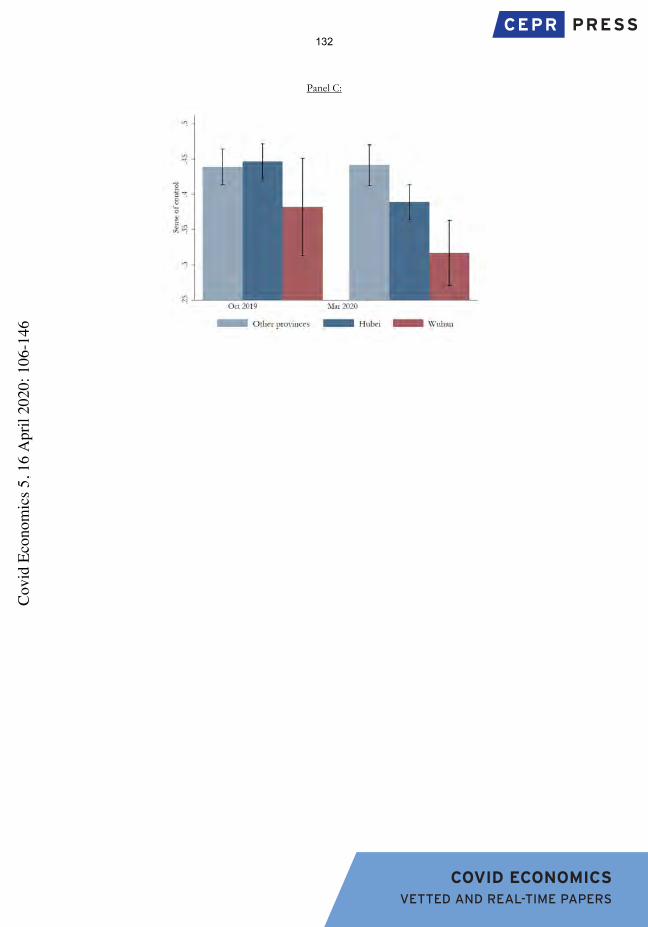
COVID ECONOMICS VETTED AND REAL-TIME PAPERS
Panel C:
132C
ovid
Eco
nom
ics 5
, 16
Apr
il 20
20: 1
06-1
46

COVID ECONOMICS VETTED AND REAL-TIME PAPERS
Figure 6: Expectations and beliefs during the Coronavirus pandemic In the following figures we plot survey measures of beliefs and expectations on financial and economic indicators. We plot responses by subjects who are quarantined in Wuhan, subjects who are quarantined in the province of Hubei (but outside of Wuhan), and subjects in different provinces in China. Expectations were elicited in March 2020 amongst a panel of student participants. We measure Panels A, B, and C with scale based survey questions, i.e., ‘compared to last year, China’s economy (your health; China’s natural environment) will become better in the next 12 months.’ The scale ranges from (1) to (5) for ‘strongly disagree’ to ‘strongly agree.’ In Panel D we ask subjects to assign probabilities to market returns from 6 scenarios and form a probability distribution. We create a measure of expected returns using the midpoints of these probability bins and plot the mean values for the Shanghai Stock Exchange index (SSE) (S&P500 and China’s GDP growth are unreported). Expected returns are for November 2019 to November 2020.
Panel A:
Panel B:
Panel C:
Panel D:
133C
ovid
Eco
nom
ics 5
, 16
Apr
il 20
20: 1
06-1
46

COVID ECONOMICS VETTED AND REAL-TIME PAPERS
Table 1: Summary statistics In Panel A, we report descriptive statistics: mean, median, min, and max for all subjects in wave one of the survey questionnaire and who also participate in wave two of the survey (225/257 subjects.). For each individual, we observe demographic characteristics detailed below from October 2019. Panel B reports characteristics by subjects who are quarantined in Wuhan (4), subjects who are quarantined in the province of Hubei (but outside of Wuhan) (3), subjects in different provinces in China (2), and a t-test of differences between subjects in Wuhan and other provinces in China (5). Panel A:
Mean Median Min Max (1) (2) (3) (4) Age 23.24 23.0 22.0 25.0 Male 0.64 1.0 0.0 1.0 Financial literacy score 2.89 3.0 0.0 5.0 Hubei Subjects 0.53 1.0 0.0 1.0 Wuhan subjects 0.09 0.0 0.0 1.0 Subjects 225
Panel B:
Full sample Other provinces Hubei Wuhan t-test (1) (2) (3) (4) (4)-(1) Age 23.24 23.19 23.30 23.24 0.00 (0.93) (0.94) (0.92) (0.94) [0.01] Male 0.64 0.63 0.64 0.71 -0.08 (0.48) (0.48) (0.48) (0.46) [-0.70] Financial literacy score 2.89 2.94 2.83 2.95 -0.07 (1.21) (1.23) (1.19) (1.24) [-0.23] Hubei subjects 0.53 0.00 1.00 1.00 - (0.50) (0.00) (0.00) (0.00) - Wuhan subjects 0.09 0.00 0.00 1.00 - (0.29) (0.00) (0.00) (0.00) - Subjects 225 106 98 21 225
134C
ovid
Eco
nom
ics 5
, 16
Apr
il 20
20: 1
06-1
46

COVID ECONOMICS VETTED AND REAL-TIME PAPERS
Table 2: Subjects’ perceptions of exposure to Coronavirus The following table reports regression results analyzing how subjects’ perceptions of exposure to Coronavirus differ by experience. Hubei subjects is an indictor variable which takes the value of one if subjects are quarantined in the Hubei province, outside of the city of Wuhan. Wuhan subjects takes the value of one if subjects are quarantined in Wuhan. The dependent variable in Column 1 an indicator variable for a survey question if there are suspected cases in the community where the subject is currently quarantined (yes/no). In Column 2 it indicates if there are confirmed cases in the community where the subject is currently (yes/no), Column 3, if there are confirmed cases among family and friends, and Column 4, if there are confirmed deaths from Coronavirus in the community where the subject is currently. The survey was taken in March 2020. Standard errors are clustered at the individual level. * p < .1, ** p < .05, *** p < .01
Dependent variable: Suspected Confirmed Family Deaths (1) (2) (3) (4) Hubei subjects 0.08** 0.14*** 0.20*** 0.02 (0.04) (0.05) (0.06) (0.03) Wuhan subjects 0.11 0.24** 0.28** 0.14 (0.08) (0.11) (0.11) (0.09) R2 0.03 0.05 0.07 0.02 Observations 225 225 225 225
Table 3: Subjects’ self-perceived fear of the Coronavirus pandemic The following table reports regression results analyzing how subjects’ perceptions of exposure to Coronavirus differ by experience. Hubei subjects is an indictor variable which takes the value of one if subjects are quarantined in the Hubei province, outside of the city of Wuhan. Wuhan subjects takes the value of one if subjects are quarantined in Wuhan. The dependent variable in Column 1 an ordinal variable for the survey question ‘do you think you are likely to be infected with COVID-19?’ Responses are on a scale between (1) and (5) for ‘very unlikely to ‘very likely.’ In Column 2 it is a question asking if the subject is afraid of the Coronavirus pandemic. Responses are on a scale between (1) and (5) for ‘not afraid at all’ to ‘very afraid.’ The survey was taken in March 2020. Standard errors are clustered at the individual level. * p < .1, ** p < .05, *** p < .01
Dependent variable: Infected Fear (1) (2) Hubei subjects 0.27 0.30* (0.17) (0.17) Wuhan subjects 0.60** 0.23 (0.28) (0.24) R2 0.02 0.01 Observations 225 225
135C
ovid
Eco
nom
ics 5
, 16
Apr
il 20
20: 1
06-1
46

COVID ECONOMICS VETTED AND REAL-TIME PAPERS
Table 4: Risk taking during the Coronavirus pandemic The following table reports regression results analyzing how risk tolerance is affected by experiencing the Coronavirus pandemic in Wuhan. In Panel A, the dependent variable is the allocation to a risky investment from a hypothetical gamble (0-1000 RMB). In Columns 1 and 3, Hubei is defined as individuals in Hubei and Wuhan (anyone in the province). In Columns 2, 4, 5, 6 it takes the value of 1 for individuals in Hubei, but outside of Wuhan. Column 1 therefore provides an estimate of the difference in the risky allocation between subjects in Wuhan and those in Hubei, whereas in Columns 2, 4, 5, 6 it is the difference between individuals in Wuhan and those in other provinces. Columns 3-4 include controls for gender, age, and financial literacy score. Column 5 (6) focuses on sub-samples of men (women). In Panel B, the explanatory variables are Hubei subjects, an indictor variable which takes the value of one if subjects are quarantined in the Hubei province. Wuhan subjects takes the value of one if subjects are quarantined in the city of Wuhan. Wave two indicates the timing of March 2020 from our second survey wave and the variables of interest are the interaction of the two location variables with the time trend. The dependent variable is a general preferences for risk index score from two survey questions on risk preferences motivated by Falk et al., (2018). The score ranges from 1 (low willingness to take risk) to 5 (high willingness to take risk) and were elicited in October 2019, and repeated in March 2020 amongst a panel of subjects in Wuhan. In Columns 3 and 7 the interaction term of Wuhan and Wave two is relative to Hubei subjects, while in Columns 4 and 8 it is relative to Other provinces. Columns 5-8 include control variables. Standard errors are clustered at the individual level. * p < .1, ** p < .05, *** p < .01
Panel A: Dependent variable: Risky allocation: March 2020 All subjects Men Women (1) (2) (3) (4) (5) (6) Hubei subjects -67.03* -67.03* -64.85 -64.85 -50.40 -88.75 (39.10) (39.10) (39.39) (39.39) (50.84) (65.61) Wuhan subjects -82.74* -149.77*** -84.99* -149.83*** -128.56** -212.24** (42.40) (45.67) (43.40) (46.34) (49.93) (102.22) Financial literacy score 7.76 7.76 13.19 -7.35 (14.85) (14.85) (20.63) (21.32) Male 7.54 7.54 - - (38.13) (38.13) Age -12.63 -12.63 -28.95 20.33 (18.91) (18.91) (22.49) (33.48) R2 0.03 0.03 0.03 0.03 0.04 0.05 Observations 225 225 225 225 145 80
Panel B:
Dependent variable: General risk preferences (1) (2) (3) (4) (5) (6) (7) (8) Wave two -0.64*** -0.59*** -0.59*** -0.59*** -0.64*** -0.60*** -0.60*** -0.60*** (0.05) (0.07) (0.07) (0.07) (0.05) (0.07) (0.07) (0.07) Hubei subjects 0.07 0.13 0.13 0.07 0.13 0.13 (0.11) (0.11) (0.11) (0.11) (0.11) (0.11) Hubei subjects x Wave two -0.09 -0.08 -0.08 -0.09 -0.08 -0.08 (0.10) (0.10) (0.10) (0.10) (0.10) (0.10) Wuhan subjects -0.35* -0.22 -0.35* -0.22 (0.19) (0.19) (0.19) (0.19) Wuhan subjects x Wave two -0.05 -0.12 -0.04 -0.12 (0.20) (0.19) (0.20) (0.19) Controls No No No No Yes Yes Yes Yes R2 0.16 0.16 0.18 0.18 0.17 0.17 0.18 0.18 Observations 450 450 450 450 450 450 450 450
136C
ovid
Eco
nom
ics 5
, 16
Apr
il 20
20: 1
06-1
46

COVID ECONOMICS VETTED AND REAL-TIME PAPERS
Table 5: Beliefs in optimism and sense of control during the Coronavirus pandemic The following table reports regression results analyzing how beliefs in individual luck are affected by experiencing the Coronavirus pandemic in Wuhan. The explanatory variables are Hubei subjects, an indictor variable which takes the value of one if subjects are quarantined in the Hubei province. Wuhan subjects takes the value of one if subjects are quarantined in the city of Wuhan. Wave two indicates the timing of March 2020 from our second survey wave and the variables of interest are the interaction of the two location variables with the time trend. The dependent variable in Panel A is an index of belief in good luck based on Darke and Freedman (1997), which ranges from 0 (low belief in personal luck) to 1 (high belief in luck). In Panel B it is an index based on questions that ask about the percentage of investors which have better luck or higher returns than you, and in Panel C an index on beliefs about subjects’ sense of control based on the Drake Beliefs about Chance Inventory (Wood and Clapham, 2005). Scores was elicited in October 2019, and repeated in March 2020 amongst a panel of student participants in Wuhan. Across panels, in Column 3 the interaction term of Wuhan and Wave two is relative to Hubei subjects, while in Column 4 it is relative to Other provinces.
Standard errors are clustered at the individual level. * p < .1, ** p < .05, *** p < .01
Panel A:
Dependent variable: Good luck (1) (2) (3) (4) Wave two -0.02*** -0.05*** -0.02*** -0.02*** (0.01) (0.01) (0.01) (0.01) Hubei subjects 0.00 -0.00 -0.00 (0.02) (0.02) (0.02) Hubei subjects x Wave two -0.07*** -0.06*** -0.06*** (0.01) (0.01) (0.01) Wuhan subjects 0.01 0.02 0.01 (0.03) (0.03) (0.03) Wuhan subjects x Wave two -0.07*** -0.04 -0.10*** (0.02) (0.03) (0.02) Controls Yes Yes Yes Yes R2 0.09 0.06 0.09 0.09 Observations 450 450 450 450
Panel B: Dependent variable: Worse luck (1) (2) (3) (4) Wave two 0.02*** 0.05*** 0.02*** 0.02*** (0.01) (0.01) (0.01) (0.01) Hubei subjects 0.01 0.01 0.01 (0.02) (0.02) (0.02) Hubei subjects x Wave two 0.06*** 0.06*** 0.06*** (0.01) (0.01) (0.01) Wuhan subjects 0.03 0.03 0.04 (0.04) (0.05) (0.04) Wuhan subjects x Wave two 0.04** 0.00 0.07*** (0.02) (0.02) (0.02) Controls Yes Yes Yes Yes R2 0.07 0.06 0.07 0.07 Observations 450 450 450 450
137C
ovid
Eco
nom
ics 5
, 16
Apr
il 20
20: 1
06-1
46
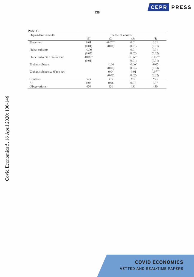
COVID ECONOMICS VETTED AND REAL-TIME PAPERS
Panel C:
Dependent variable: Sense of control (1) (2) (3) (4) Wave two 0.01 -0.02*** 0.01 0.01 (0.01) (0.01) (0.01) (0.01) Hubei subjects -0.00 0.01 0.01 (0.02) (0.02) (0.02) Hubei subjects x Wave two -0.06*** -0.06*** -0.06*** (0.01) (0.01) (0.01) Wuhan subjects -0.06 -0.06* -0.05 (0.04) (0.04) (0.04) Wuhan subjects x Wave two -0.04* -0.01 -0.07*** (0.02) (0.02) (0.02) Controls Yes Yes Yes Yes R2 0.06 0.06 0.07 0.07 Observations 450 450 450 450
138C
ovid
Eco
nom
ics 5
, 16
Apr
il 20
20: 1
06-1
46

COVID ECONOMICS VETTED AND REAL-TIME PAPERS
Table 6: Expectations and beliefs during the Coronavirus pandemic The following table reports regression results analyzing how expectations and beliefs on aggregate outcomes differ by experience. Hubei subjects is an indictor variable which takes the value of one if subjects are quarantined in the Hubei province, outside of the city of Wuhan. Wuhan subjects takes the value of one if subjects are quarantined in Wuhan. Expectations were elicited in March 2020 amongst a panel of student participants in Wuhan. The dependent variable in Column 1 (2) (3) are scale-based survey questions, i.e., ‘compared to last year, China’s economy (your health; China’s natural environment) will become better in the next 12 months.’ The scale ranges from (1) to (5) for ‘strongly disagree’ to ‘strongly agree.’ Column 4 asks subjects to assign probabilities to market returns from 6 scenarios and form a probability distribution. We create a measure of expected returns using the midpoints of these probability bins and plot the mean values for the Shanghai Stock Exchange index (SSE). Expected returns are for November 2019 to November 2020. Standard errors are clustered at the individual level. * p < .1, ** p < .05, *** p < .01
Dependent variable: Economy Health Environment SSE (1) (2) (3) (4) Hubei subjects -0.30* -0.48*** -0.43*** -0.02 (0.16) (0.17) (0.16) (0.02) Wuhan subjects -0.47** -0.62** -0.84*** -0.03 (0.22) (0.28) (0.23) (0.02) Controls Yes Yes Yes Yes R2 0.03 0.06 0.07 0.02 Observations 225 225 225 225
139C
ovid
Eco
nom
ics 5
, 16
Apr
il 20
20: 1
06-1
46

COVID ECONOMICS VETTED AND REAL-TIME PAPERS
Appendix for
“Risk Taking during a Global Crisis: Evidence from Wuhan”
Appendix Figure 1: October 2019 survey sessions in Wuhan, China The figures below show pencil and paper survey wave one sessions at WUST in October 2019.
140C
ovid
Eco
nom
ics 5
, 16
Apr
il 20
20: 1
06-1
46

COVID ECONOMICS VETTED AND REAL-TIME PAPERS
141C
ovid
Eco
nom
ics 5
, 16
Apr
il 20
20: 1
06-1
46

COVID ECONOMICS VETTED AND REAL-TIME PAPERS
Appendix Figure 2: Online survey conducted in March 2020 The figures below shows an example screen from the online wave two survey (translated into English) while subjects are in quarantined.
142C
ovid
Eco
nom
ics 5
, 16
Apr
il 20
20: 1
06-1
46

COVID ECONOMICS VETTED AND REAL-TIME PAPERS
Appendix Table 1: Risk allocation during the Coronavirus pandemic The following table reports regression results analyzing how risk tolerance is affected by experiencing the Coronavirus pandemic in Wuhan. The dependent variable is the allocation to a risky investment from a hypothetical gamble (0-1000 RMB). In Columns 1, 3, 5, and 7 Hubei is defined as individuals in Hubei and Wuhan (anyone in the province). In Columns 2, 4, 6, and 8 the variable Hubei takes the value of 1 for individuals in Hubei, but outside of Wuhan. In Columns 1-2 the risky allocation variable is our baseline measure where we recode 13 observations with missing values in the risky lottery, but 1000 allocated to the safe lottery as zero. In Columns 3-4 we omit 4 observations where the risky allocation was stated as greater than 1000 (these are top coded to 1000 in Columns 1-2). In Columns 5-6 we omit these top coded observations. In Columns 7-8 we omit all of the previous mentioned observations. Standard errors are clustered at the individual level. * p < .1, ** p < .05, *** p < .01
Dependent variable: Risky allocation: March 2020 (1) (2) (3) (4) (5) (6) (7) (8) Hubei subjects -64.85 -64.85 -55.37 -55.37 -66.37* -66.37* -62.52 -62.52 (39.39) (39.39) (35.58) (35.58) (37.38) (37.38) (39.99) (39.99) Wuhan subjects -84.99* -149.83*** -69.99* -125.36*** -79.28* -145.65*** -89.11* -151.63*** (43.40) (46.34) (41.58) (45.11) (42.07) (45.81) (45.80) (48.07) Controls Yes Yes Yes Yes Yes Yes Yes Yes R2 0.03 0.03 0.03 0.03 0.03 0.03 0.03 0.03 Observations 225 225 221 221 225 225 212 212
143C
ovid
Eco
nom
ics 5
, 16
Apr
il 20
20: 1
06-1
46

COVID ECONOMICS VETTED AND REAL-TIME PAPERS
Appendix Table 2: Risk allocation during the Coronavirus pandemic The following table reports regression results analyzing how risk tolerance is affected by experiencing the Coronavirus pandemic in Wuhan. The dependent variable is the allocation to a risky investment from a hypothetical gamble (0-1000 RMB). We control for the October 2019 to March 2020 change in general risk preference score as well as changes in optimism and beliefs in luck. In Columns 4-6 the variable Hubei takes the value of 1 for individuals in Hubei, but outside of Wuhan. Standard errors are clustered at the individual level. * p < .1, ** p < .05, *** p < .01
Dependent variable: Risky allocation: March 2020 (1) (2) (3) (4) (5) (6) Decrease in risk tolerance score -61.49 -66.24 -66.22 -61.09 -63.58 -64.83 (45.96) (44.34) (44.04) (45.16) (43.54) (43.57) Decrease in beliefs in good luck -33.41 -4.06 (40.27) (40.20) Increase in beliefs of worse luck -7.19 41.42 (38.14) (40.50) Decrease in control over luck -4.07 29.65 (36.77) (39.28) Hubei subjects -62.02 -82.01** -73.64* (39.15) (41.50) (42.37) Wuhan subjects -142.84*** -166.97*** -156.32*** (48.17) (50.01) (48.17) Control variables Yes Yes Yes Yes Yes Yes R2 0.02 0.02 0.02 0.04 0.05 0.05 Observations 225 225 225 225 225 225
144C
ovid
Eco
nom
ics 5
, 16
Apr
il 20
20: 1
06-1
46

COVID ECONOMICS VETTED AND REAL-TIME PAPERS
Online Appendix A: Sample survey questions translated into English
Belief on good luck Darke and Freedman (1997)
Likert-scale which ranges from strongly disagree (1) … strongly agree (5).
Some people are consistently lucky, and others are unlucky. I consider myself to be a lucky person. I believe in luck. I often feel like it’s my lucky day. Nobody can win at games of chance in the long-run. I consistently have good luck. It’s a mistake to base any decisions on how lucky you feel. Luck works in my favour, especially this year. I don’t mind leaving things to chance because I’m a lucky person. Even the things in life I can’t control tend to go my way because I’m lucky. In general I am lucky. There is such a thing as luck that favours some people, but not others. Luck is nothing more than random chance.
Beliefs about luck
If you make investment on stocks this year, what percentage of other investors have better luck than you at investing stocks with above average performance? (Please give a number between 0% and 100%)
If you make investment on stocks this year, what percentage of other investors had higher returns than you? (Please give a number between 0% and 100%)
Control over luck Drake Beliefs about Chance Inventory; Wood and Clapham (2005)
Participants indicate the extent of their agreement using Likert-scale which ranges from strongly disagree (1) … strongly agree (5).
If I well prepared, I would have very large likelihood to win a gamble. Some gamblers are just born lucky. The longer I’ve been losing, the more likely I am to win. The chances of winning a substantial amount of money at the Casino are quite high I think I’ll win a good prize in sport lottery (over $10,000) one day One day I’m going to strike it lucky at gambling If I concentrated hard enough I might be able to influence whether I win when I play the pokies I can/could stick to a budget when/if I gamble
Risk taking Falk et al., (2018)
Risk measures were elicited through two qualitative questions and one quantitative question:
In general, how willing are you to take risks? On a scale of 1(not willing at all) - 5(very willing to)
Will you take more risk this year compared to last year? On a scale of 1(less risk) - 5 (more risk)
Imagine you have an extra 1,000 yuan in your pocket, and you have to options with how to use it:
145C
ovid
Eco
nom
ics 5
, 16
Apr
il 20
20: 1
06-1
46
COVID ECONOMICS VETTED AND REAL-TIME PAPERS
a. Use an amount of the money to invest in a lottery (with a 50% chance that you can win up to 2,000 yuan (including the principal of 1,000 yuan), and a 50% chance of zero additional winnings)
b. Don’t make any investment.
Please fill in the following boxes how you will allocate the 1,000 yuan in these two options:
_____Yuan in lottery investments _____ Yuan in keep in cash
Economy expectations
All questions on scale of strongly disagree (1) … strongly agree (5). Compared to last year, China’s economy will become better in the next 12 months Compared with last year, my health will be better in the next 12 months Compared with last year, China’s natural environment will become better in the next 12 months
Stock market expectations
Stock market expectations: in the following we present you with 6 scenarios of how the annual percentage change of stock indices could be during this year (between Nov 2020-Nov 2021). Please indicate how likely you think the individual scenarios are. Assign a probability to each of the scenarios, and make sure the sum of the probability to be 100%. Shanghai Stock exchange index
-20% -10-20% 0-10% 0 +10 % 10-20% +20%
Questions on trust WVS; Kosse et al., (2020) All questions on scale of strongly disagree (1) … strongly agree (5).
In general, the vast majority of people in the society can be trusted In general, no one else can be trusted, I can only rely on myself We’d better stay vigilant when dealing with strangers Others treat me with good intentions Additional questions Are there confirmed COVID-19 cases among your family member and friends? Yes/no Are there any confirmed COVID-19 cases in the community where you currently live? Yes/no Are there any suspected cases in the community where you currently live? Yes/no Has anyone in your community died from the COVID-19? Yes/no Are you afraid of this epidemic?
1)Not afraid at all …… 5)Very afraid Do you think you are likely to be infected with COVID-19?
1)Very unlikely …… 5)Very likely
146C
ovid
Eco
nom
ics 5
, 16
Apr
il 20
20: 1
06-1
46

COVID ECONOMICS VETTED AND REAL-TIME PAPERS
Covid Economics Issue 5, 16 April 2020
The case for universal cloth mask adoption and policies to increase the supply of medical masks for health workers
Jason Abaluck,1 Judith Chevalier,2 Nicholas A. Christakis,3 Howard Forman,4 Edward H. Kaplan,5 Albert Ko6 and Sten H. Vermun7
Date submitted: 7 April 2020; Date accepted: 8 April 2020
We recommend the immediate universal adoption of cloth facemasks, including homemade masks, and accompanying policies to increase the supply of medical masks for health workers. Universal adoption will likely slow the spread of the Covid-19 virus by reducing transmission from asymptomatic individuals. We provide strongly suggestive evidence from cross-country data that facemask use slows the growth rate of cases and deaths. This complements extant scientific data on mask usage. Our analysis suggests each cloth facemask generates thousands of dollars in value from reduced mortality risk. Each medical mask, when used by a healthcare worker, may generate millions of dollars in value, and policies to encourage greater production prioritised for health workers are urgently needed.
1 Associate Professor of Economics, Yale School of Management.2 William S Beinecke Professor of Economics and Finance, Yale School of Management.3 Sterling Professor of Social and Natural Science, Yale University.4 Professor of Radiology and Biomedical Imaging, Economics, and Public Health (Health Policy); Professor in
the Practice of Management, Yale School of Management.5 William N. and Marie A. Beach Professor of Operations Research, Yale School of Management; Professor of
Public Health, Yale School of Public Health; Professor of Engineering, Yale University.6 Professor of Epidemiology and Medicine and Department Chair, Epidemiology of Microbial Diseases, Yale
School of Public Health.7 Dean and Anna M.R. Lauder Professor of Public Health, Yale School of Public Health; Professor of Pediatrics,
Yale School of Medicine.
147C
ovid
Eco
nom
ics 5
, 16
Apr
il 20
20: 1
47-1
59

COVID ECONOMICS VETTED AND REAL-TIME PAPERS
Introduction
The urgent need to stop the spread of COVID-19 is among the most important health policy challenges of our lifetimes. Millions of lives are at stake globally, and the economic security of tens of millions of Americans is threatened. In this paper, we review briefly the scientific literature on mask evidence, undertake an empirical analysis of mask efficacy, and estimate the economic value of universal cloth mask-wearing. We find, using fairly conservative estimates of mask efficacy, that this policy could have very large benefits. However, given the enormous importance of hospital-grade mask access for healthcare workers, our findings about universal mask-wearing must be coupled with policies to increase the supply of such protective equipment for healthcare workers. We estimate that the benefits of universal cloth facemask adoption in the US is conservatively in the $3,000-$6,000 range per household due to the impact of masks in slowing the spread of the virus. The benefits of each medical mask for healthcare personnel may be hundreds of times larger, and there is an ethical imperative to safeguard frontline healthcare workers. Thus, public policy ideally would both encourage universal mask adoption and deal with the urgent policy priority that front-line healthcare workers face shortages of personal protective equipment, such as N95 respirators and surgical masks. Until very recently, the United States Centers for Disease Control and the US Surgeon General’s Office discouraged mask-wearing. As of this writing, the World Health Organization (WHO) discourages mask-wearing by the general public. This is due in part to the shortage of protective equipment for healthcare workers as well as the limited evidence that non-medical masks protect the wearer from infection.1 Thus, masks are currently only recommended by WHO (and formerly by the CDC) for healthcare workers, and in some circumstances, for symptomatic individuals while receiving care.
However, there is broad agreement about two crucial points:
1 For example, Dr. Jerome Adams, the Surgeon General, tweeted on February 29, “They are NOT effective in preventing general public from catching #Coronavirus, but if healthcare providers can’t get them to care for sick patients, it puts them and our communities at risk!” (https://twitter.com/surgeon_general/status/1233725785283932160) . The Surgeon General confirmed in an interview on April 1 that the Surgeon General’s office has asked the CDC to reevaluate this advice. On April 3, the CDC recommended cloth face coverings and on April 4, the Surgeon General posted a video demonstrating how to make a cloth face covering.
148C
ovid
Eco
nom
ics 5
, 16
Apr
il 20
20: 1
47-1
59
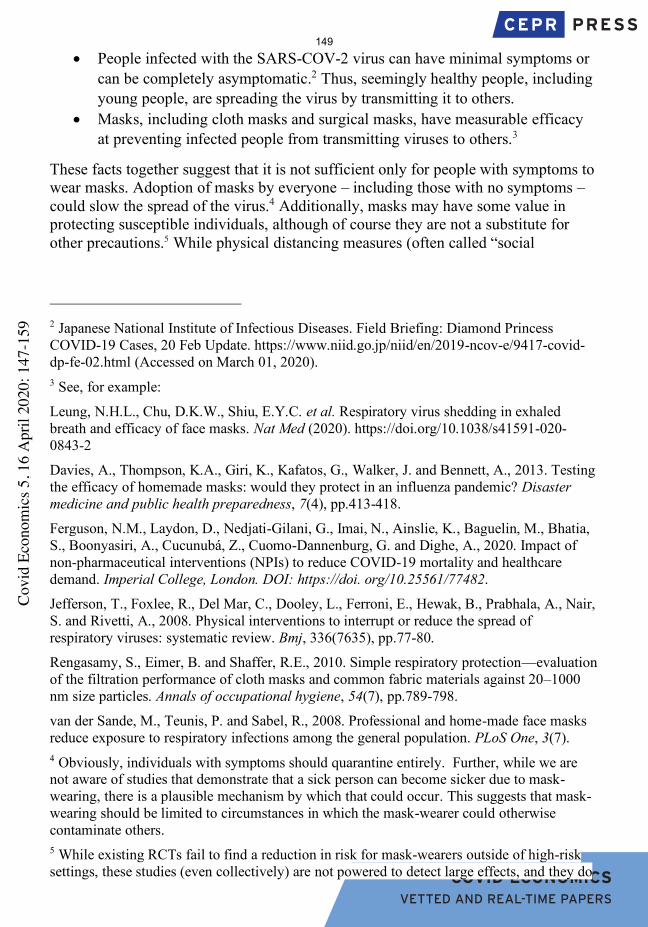
COVID ECONOMICS VETTED AND REAL-TIME PAPERS
• People infected with the SARS-COV-2 virus can have minimal symptoms or can be completely asymptomatic.2 Thus, seemingly healthy people, including young people, are spreading the virus by transmitting it to others.
• Masks, including cloth masks and surgical masks, have measurable efficacy at preventing infected people from transmitting viruses to others.3
These facts together suggest that it is not sufficient only for people with symptoms to wear masks. Adoption of masks by everyone – including those with no symptoms – could slow the spread of the virus.4 Additionally, masks may have some value in protecting susceptible individuals, although of course they are not a substitute for other precautions.5 While physical distancing measures (often called “social
2 Japanese National Institute of Infectious Diseases. Field Briefing: Diamond Princess COVID-19 Cases, 20 Feb Update. https://www.niid.go.jp/niid/en/2019-ncov-e/9417-covid-dp-fe-02.html (Accessed on March 01, 2020). 3 See, for example:
Leung, N.H.L., Chu, D.K.W., Shiu, E.Y.C. et al. Respiratory virus shedding in exhaled breath and efficacy of face masks. Nat Med (2020). https://doi.org/10.1038/s41591-020-0843-2
Davies, A., Thompson, K.A., Giri, K., Kafatos, G., Walker, J. and Bennett, A., 2013. Testing the efficacy of homemade masks: would they protect in an influenza pandemic? Disaster medicine and public health preparedness, 7(4), pp.413-418.
Ferguson, N.M., Laydon, D., Nedjati-Gilani, G., Imai, N., Ainslie, K., Baguelin, M., Bhatia, S., Boonyasiri, A., Cucunubá, Z., Cuomo-Dannenburg, G. and Dighe, A., 2020. Impact of non-pharmaceutical interventions (NPIs) to reduce COVID-19 mortality and healthcare demand. Imperial College, London. DOI: https://doi. org/10.25561/77482.
Jefferson, T., Foxlee, R., Del Mar, C., Dooley, L., Ferroni, E., Hewak, B., Prabhala, A., Nair, S. and Rivetti, A., 2008. Physical interventions to interrupt or reduce the spread of respiratory viruses: systematic review. Bmj, 336(7635), pp.77-80.
Rengasamy, S., Eimer, B. and Shaffer, R.E., 2010. Simple respiratory protection—evaluation of the filtration performance of cloth masks and common fabric materials against 20–1000 nm size particles. Annals of occupational hygiene, 54(7), pp.789-798.
van der Sande, M., Teunis, P. and Sabel, R., 2008. Professional and home-made face masks reduce exposure to respiratory infections among the general population. PLoS One, 3(7). 4 Obviously, individuals with symptoms should quarantine entirely. Further, while we are not aware of studies that demonstrate that a sick person can become sicker due to mask-wearing, there is a plausible mechanism by which that could occur. This suggests that mask-wearing should be limited to circumstances in which the mask-wearer could otherwise contaminate others. 5 While existing RCTs fail to find a reduction in risk for mask-wearers outside of high-risk settings, these studies (even collectively) are not powered to detect large effects, and they do
149C
ovid
Eco
nom
ics 5
, 16
Apr
il 20
20: 1
47-1
59

COVID ECONOMICS VETTED AND REAL-TIME PAPERS
distancing”) are of paramount importance in preventing the spread of the virus, they cannot be fully enforced. People interact at close quarters when they perform essential activities such as buying food or seeking healthcare, and cashiers or delivery workers may interact with hundreds of people a day. Preventing the transmission of the virus from asymptomatic individuals in such cases is likely the principal benefit of broader mask adoption. For example, in settings in which a worker interacts with the public, both the worker and the public are safer if the other party is wearing a mask. An important concern is the hoarding of medical masks before there is adequate supply for front-line medical workers. Non-medical alternatives should therefore be considered. For example, there is scientific evidence that homemade cloth masks can lessen viral transmission.6 Encouraging production of cloth masks may help counteract and discourage medical mask hoarding; this can include homemade production and perhaps industrial production, but only to the extent that supply chains do not interfere with those for critically important medical masks. People equipped with cloth masks may feel more comfortable donating existing respirators and surgical masks to medical personnel and first responders. Thus, encouraging the production of cloth masks, including homemade masks, could help protect healthcare workers. Due to the serious concern that any mask recommendation will lead the public to demand more surgical and N95 respirators, any recommendation for broader mask use should be coupled with policies designed to improve their availability to healthcare workers, including subsidies, invoking the Defense Production Act (DPA) in the United States and similar policies elsewhere, and mandating that orders of medical masks from healthcare workers must be given absolute priority.
The Economic Value of Masks The extant literature examines mask efficacy largely in laboratory and clinical settings. Measures of the potential reduction in the overall transmission of COVID-19 in the field are lacking. To supplement the existing laboratory and medical evidence and find measures to compute the overall value of masks, we need to know by how much masks impede the transmission of the SARS-COV-2 virus and the value of reductions in transmission. To analyze the impact of masks on viral transmission, we consider the relationship between norms of mask-use and viral spread at the country level, controlling for other policy factors.
not address at all the critical question of whether masks prevent transmission of the virus from infected individuals (Cowling et. al. 2009, MacIntyre and Chunghtai 2015). 6 See van der Sande et. al. 2008, Rengasamy et. al. 2010, Davies et. al. 2013.
150C
ovid
Eco
nom
ics 5
, 16
Apr
il 20
20: 1
47-1
59

COVID ECONOMICS VETTED AND REAL-TIME PAPERS
Figure 1 shows confirmed positive tests for COVID-19 in all countries with at least 5 million people for which at least 8 days of data are available after the first day with 100 reported cases (select countries are labeled).7 Time 0 is the first day with 100 cases, and the figure shows the progress of the epidemic thereafter. Countries with pre-existing norms that all sick people wear masks are shown with a solid black line, countries which do not, but later required masks for infected individuals or the whole population are shown with a dotted line, and countries with no mask norm and no official recommendation as of March 29, 2020 are shown in light grey.
Figure 1: Confirmed Positive Tests Since 100 Cases
The pattern in the figure is quite stark: countries with pre-existing norms that sick people should wear masks – including South Korea, Japan, Hong Kong and Taiwan – have been among the most effective at containing the spread of the epidemic. The average daily growth rate of confirmed positives is 18% in countries with no pre-existing mask norms and 10% in countries with such norms.8 This evidence is far from definitive: norms do not perfectly predict actual mask availability and use, these countries may have instituted other policies which
7 The data used in Figure 1 are taken from the COVID-19-Israel Data Repository, https://github.com/COVID-19-Israel/Covid-19-data (Accessed on April 1st, 2020). Jason Abaluck undertook the regression analysis and we are grateful for the research assistance of Emily Crawford. 8 The “dotted-line” countries which imposed stronger requirements on mask use typically did not do so until the epidemic was well-developed, so we would not expect to see an effect in the graph.
Belgium
China
Egypt
France
Germany
Greece
Hong Kong
India
Iran
Ireland
Israel
Japan
Malaysia
Singapore
S. Korea
Spain
Sweden
Taiwan
Thailand
USA
UK
Austria
Czechia Australia
Italy
Bulgaria
Romania
Switzerland
100
1,000
10,000
100,000
0 2 4 6 8 10 12 14 16 18 20 22 24 26 28 30
Nu
mb
er
of
Ca
ses
Number of Days
151C
ovid
Eco
nom
ics 5
, 16
Apr
il 20
20: 1
47-1
59

COVID ECONOMICS VETTED AND REAL-TIME PAPERS
contained the spread of the epidemic (such as widespread testing in South Korea), and infection rates are imperfectly measured and may appear higher in countries with more testing among other factors.
Table 1
To aid in interpreting the graph, we conduct several regression analyses, shown in Table 1. The goal of this analysis is to examine whether mask norms have a relationship to case growth, controlling for other factors. Column (1) shows the measured relationship between the growth rate of cases and an indicator variable for countries with pre-existing mask norms. In Column (2), we control for the timing of school closings, workplace closings, the cancellation of public events and the closing of public transport as “Baseline Policy Controls”. Specifically, specifications with “Baseline Policy Controls” control for policies in place at time 0 (100 cases or 10 deaths). Column 3 undertakes a more dynamic view of policy variables. In this specification, “Average Policy over 8 Days” adds controls for these same policy variables, but averaged over the first 8 days after time 0. When adding these controls we find that the estimated effect of masks is unchanged or grows slightly larger.9 In column (4), we control for an “Asia” fixed effect since growth rates may differ due to cultural differences common to Asian countries; the estimated effect on cases is slightly larger with this control.
9 These policy variables come from the Oxford COVID-19 Government Response Tracker, https://www.bsg.ox.ac.uk/research/research-projects/oxford-covid-19-government-response-tracker (Accessed on March 30th, 2020).
152C
ovid
Eco
nom
ics 5
, 16
Apr
il 20
20: 1
47-1
59

COVID ECONOMICS VETTED AND REAL-TIME PAPERS
One measurement concern is that cases are measured with error and rates of testing and measurement vary across countries. Thus, deaths from COVID-19 may be better measured than cases. We repeat the analyses above using deaths as the outcome variable in the right panel of Table 1. We find that the growth rate of deaths is 21% in countries with no mask norms and 11% in countries with such norms. Even with the small number of observations, the impact of masks in all reported analyses is statistically significant at the 5% level, and usually at the 1% level. While we control for major policy variables, there are many factors that cannot be controlled for in an ecological study of this type.10 These results are far from the final word, but they do complement and provide a measure of external validity the epidemiological studies of masks cited above. While our analysis principally concerns the impact of norms that sick people wear masks, it has direct implications for universal mask adoption. If the causal interpretation of the above results is correct, the impact of mask norms (which increase the likelihood of mask wearing relative to no norm countries) should understate the impact of universal mask adoption for both visibly sick and healthy individuals (who are potentially asymptomatically infected). Our economic analysis suggests that that even if masks are far less effective than the evidence above suggests, the potential benefits are substantial. If masks reduce the transmission rate of the virus by only 10%, epidemiological models suggest that hundreds of thousands of deaths could be prevented globally,11 creating trillions of dollars in economic value. According to one commonly used epidemiological model, a 10% reduction in transmission probabilities would generate $3,000-6,000 in value per household from reduced mortality risk in the US alone.12 This estimate is conservative with respect to the benefits, as it does not include the economic benefits from a quicker resumption of normal activity. And our estimates above suggest that the effect of masks could be 5-6 times as large. Of course, all such estimates are only as reliable as the underlying epidemiological models. But even if these models overstated risk by a factor of ten, the benefits of cloth masks, would conservatively be $300 per household.
10 For example, in addition to norms of mask wearing, handshakes are rare in Japan which may slow the spread of the virus. However, one comment that is often made is that a variety of factors may distinguish the Asian countries from the non-Asian countries. Including an indicator for “Asian” actually increases our estimates of the case reduction from mask norms. 11 Ferguson et. al. suggests that a 10% reduction in viral transmission probabilities (and thus R) would reduce by about 10% total deaths from COVID-19 through October. 12 Greenstone and Nigam (2020) estimate that the total mortality risk from the virus is $60,000 per household. From Ferguson et. al., a 10% reduction in transmission probability would lead to 10% lower mortality risk, giving $6,000 per household. With social distancing measures in place, the reduction in mortality risk would be $3,000 per household (based on the estimate in Greenstone and Nigam that social distancing reduces mortality risk by ½).
153C
ovid
Eco
nom
ics 5
, 16
Apr
il 20
20: 1
47-1
59
COVID ECONOMICS VETTED AND REAL-TIME PAPERS
Our analysis considers the adoption of masks in addition to social distancing. However, masks may also play a role in the eventual transition from the current extreme social distancing. In a report whose coauthors include former FDA Commission Scott Gottlieb, former FDA Commissioner and former administrator for the Centers for Medicare and Medicaid Services Mark McClellan, former FDA Chief of Staff Lauren Silvis, and Johns Hopkins Center for Health Security Faculty Caitlin Rivers and Crystal Watson, the authors argue that the eventual transition from the current extreme social distancing should involve universal wearing of cloth masks. Dr. Gottlieb argues in a recent interview, "if you mandated that the entire population had to wear a mask when they went out, all those asymptomatic carriers that are now transmitting it through respiratory droplets… it would be much harder for them to transmit it."13 Note that all of our arguments for the value of masks for the average person are magnified many times when we consider the current value of medical masks such as N95 respirators for healthcare workers.14 First, healthcare workers are especially exposed to the virus if they lack protection: they cannot socially distance from their patients, they interact with a large number of patients, and those patients are especially likely to be exposed. Second, if infected, healthcare workers without adequate protection are especially likely to expose others for similar reasons. Third, the people healthcare workers interact with are especially likely to have pre-existing medical conditions and thus high mortality rates from the virus. Fourth, there is substantial evidence that N95 respirators and surgical masks protect healthy individuals, and that N95 respirators are most effective since medical procedures can lead to the aerosolization of droplets which makes medical masks essential.15 Fifth, as discussed previously, medical masks are extremely effective at preventing infected healthcare workers from transmitting the virus. Sixth, keeping healthcare workers healthy during a pandemic is especially critical to prevent healthcare facilities from being overwhelmed, increasing mortality.16 Multiplying these factors together, the social value of each N95 mask for a healthcare worker could easily be more than a
13 See Gottlieb, Scott, et. al. (2019) for the report. The interview can be found at Moreno, E., “Former FDA Commissioner Mulls Mask Requirements for Some Age Groups in Public”, The Hill, March 18, 2020. 14 Yan, J., Guha, S., Hariharan, P. and Myers, M., 2019. Modeling the Effectiveness of Respiratory Protective Devices in Reducing Influenza Outbreak. Risk Analysis, 39(3), pp.647-661. 15 Long, Y., Hu, T., Liu, L., Chen, R., Guo, Q., Yang, L., Cheng, Y., Huang, J. and Du, L., 2020. Effectiveness of N95 respirators versus surgical masks against influenza: A systematic review and meta‐analysis. Journal of Evidence‐Based Medicine. 16 Fong, M.W., Gao, H., Wong, J.Y., Xiao, J., Shiu, E.Y., Ryu, S. and Cowling, B.J., 2020. Nonpharmaceutical Measures for Pandemic Influenza in Nonhealthcare Settings-Social Distancing Measures. Emerging infectious diseases, 26(5).
154C
ovid
Eco
nom
ics 5
, 16
Apr
il 20
20: 1
47-1
59

COVID ECONOMICS VETTED AND REAL-TIME PAPERS
million dollars per mask on the margin.17 This calculation illustrates the tremendous value of subsidizing the production of medical masks. This calculation, clearly, is in addition to the moral imperative to protect healthcare workers during this crisis.
Homemade Masks as an Antidote to Hoarding
Our read of the disparity between the scientific evidence for masks and the (now changing) public discourse on masks is that policymakers were and are rightly concerned that an emphasis on the private benefits of wearing masks will lead to hoarding of commercially-produced masks reducing availability in the healthcare system. However, we believe that an emphasis on the social benefits of mask-wearing and an emphasis on the wearing of homemade masks by the public could lead to a substantial fraction of the health benefits without the negative impacts of mask hoarding. An example of a socially influenced mask movement is the Czech Republic. In the Czech Republic, homemade mask-making was led by celebrity influencers, and the country went from masks being unusual to being nearly universal in 10 days.18 We are also concerned that some recent media and other reports have emphasized the private benefits of mask-wearing (that is, infection protection to the wearer) without discussing the efficacy of non-medical fabric face masks in lowering transmission.19 This could exacerbate existing supply shortages for hospital-quality masks. Healthcare leaders can responsibly respond to this information by emphasizing the relative efficacy of cloth masks in preventing transmission and the need to increase home production or production by textile companies not previously engaged in making health products.
17 The value of the above parameters is difficult to know, as in normal times, healthcare workers would not operate without protective equipment. To take one back of the envelope calculation, if healthcare workers are 10 times as likely to become infected without adequate protection, three times as likely to infect others, encounter patients with a 6x higher mortality rate than the average person, our $6,000 value above would translate to more than $1 million per mask. 18 See https://www.youtube.com/watch?v=HhNo_IOPOtU&feature=youtu.be. 19 See, for example, the recent New York Times Op Eds, Tupekci,, Zeynep, “Why Telling People they don’t need masks Backfired”, New York Times, March 17, 2020 or Sheikh, Knvul, “More Americans Should Probably Wear Masks for Protection”, March 27, 2020.
155C
ovid
Eco
nom
ics 5
, 16
Apr
il 20
20: 1
47-1
59

COVID ECONOMICS VETTED AND REAL-TIME PAPERS
Policy Recommendations
Given the evidence of the benefits of universal mask-wearing and the urgent need for medical masks for health workers, we have two principal recommendations. Political officials should:
Additionally, political officials can and should lead by:
• Themselves wearing cloth masks in public at all times. If these masks are obviously homemade, this will emphasize the pro-social benefits of protecting both healthcare workers (who need commercial masks) and the public at large.
1) Promote every market and policy lever to increase the production of medical grade masks and guarantee adequate supply for healthcare workers.
o Suppliers who produce and sell medical masks should be heavily rewarded. State and federal governments should authorize large subsidies for medical masks. This will expand manufacturing capacity while increasing the affordability of medical masks for healthcare providers. Subsidies many times greater than the usual price of masks are called for to properly incentivize production.
o Priority for all mask orders should be given to medical personnel, using fines or other penalties for manufacturers who fail to prioritize such orders.
o The Defense Production Act should be invoked to increase production of medical grade masks. However, care must be taken to heavily reward private firms who efficiently produce medical masks or the concurrent supply from the private market will be undermined.
o Technologies and strategies for mask sterilization or reprocessing should be developed and deployed as a stopgap until sufficient N95 masks are available for all health workers.
2) Emphasize that everyone should make and wear cloth masks in public at all times, not just those with symptoms. Once surgical masks are no longer in short supply, encourage the universal adoption of these higher-quality protective devices.
156C
ovid
Eco
nom
ics 5
, 16
Apr
il 20
20: 1
47-1
59
COVID ECONOMICS VETTED AND REAL-TIME PAPERS
• Emphasizing that mask wearing is a complement to other social distancing measures, not a substitute. 20 Mask wearers who violate social distancing recommendations continue to place themselves and others at high risk.
• Supporting or requiring mask-wearing in essential services such as grocery stores where employees have many contacts in a day.
• Emphasizing that one of the main goals of mask wearing is to protect others (As we have seen from the recent spate of COVID-19 cases among public officials, it is reasonable for asymptomatic public officials to behave as if they are at constant risk of infecting the public and to take precautions in their interactions with others).
• Reaching out to visible persons such as media members and strongly encouraging them to do the same.
• Encouraging and demonstrating the correct production and use of homemade masks.
• Providing public health messages with mask-making instructions and instructions on fit. For example, one of the limitations of homemade masks identified by Davies et. al. (2013) is the poor fit achieved by amateur mask-makers. For example, public health instructions would inform individuals with beards to trim the beard to achieve the best fit. Mask users should also be instructed to wash hands after removing masks and wash or dispose of masks after repeated use.
• Partnering with non-medical mask industry to provide free or reduced-price cloth masks to everyone.
Conclusion
The economic case for universal mask wearing is convincing and urgent, but the moral need to provide adequate equipment to frontline healthcare workers is an even higher imperative. Enacting policies to increase medical mask production, and concurrently encouraging the widespread production and use of cloth masks can achieve both objectives. Public officials should encourage and support universal cloth mask adoption immediately. These masks should be dust-prevention quality (as sold in hardware stores) or home-made fabric masks that are worn snugly) until which time as surgical or N95 masks are no longer in short supply. Outside of crises, policies do not exist where a few dollars of expenditure per person can produce thousands of dollars in benefit. We are in a rare moment when such benefits are achievable--this is an urgent crisis and action is necessary.
20 See, Pourbohloul, B., et.al. 2005 for a discussion of the relative efficacy of various control strategies.
157C
ovid
Eco
nom
ics 5
, 16
Apr
il 20
20: 1
47-1
59

COVID ECONOMICS VETTED AND REAL-TIME PAPERS
References to Academic Articles
Cowling, B.J., Chan, K.H., Fang, V.J., Cheng, C.K., Fung, R.O., Wai, W., Sin, J., Seto, W.H., Yung, R., Chu, D.W. and Chiu, B.C., 2009. Facemasks and hand hygiene to prevent influenza transmission in households: a cluster randomized trial. Annals of internal medicine, 151(7), pp.437-446. Davies, A., Thompson, K.A., Giri, K., Kafatos, G., Walker, J. and Bennett, A., 2013. Testing the efficacy of homemade masks: would they protect in an influenza pandemic? Disaster medicine and public health preparedness, 7(4), pp.413-418. Ferguson, N.M., Laydon, D., Nedjati-Gilani, G., Imai, N., Ainslie, K., Baguelin, M., Bhatia, S., Boonyasiri, A., Cucunubá, Z., Cuomo-Dannenburg, G. and Dighe, A., 2020. Impact of non-pharmaceutical interventions (NPIs) to reduce COVID-19 mortality and healthcare demand. Imperial College, London. DOI: https://doi. org/10.25561/77482.
Fong, M.W., Gao, H., Wong, J.Y., Xiao, J., Shiu, E.Y., Ryu, S. and Cowling, B.J., 2020. Nonpharmaceutical Measures for Pandemic Influenza in Nonhealthcare Settings-Social Distancing Measures. Emerging infectious diseases, 26(5). Gottlieb, S., Rivers, C., McClellan, M.B., Silvis, L., and Watson, C., “National Coronavirus Response: A Road Map to Reopening,” American Enterprise Institute, March 28, 2020. Greenstone, M. and Nigam, V. 2020. Does Social Distancing Matter? BFI Working Paper, No 2020-26. Jefferson, T., Foxlee, R., Del Mar, C., Dooley, L., Ferroni, E., Hewak, B., Prabhala, A., Nair, S. and Rivetti, A., 2008. Physical interventions to interrupt or reduce the spread of respiratory viruses: systematic review. Bmj, 336(7635), pp.77-80. Long, Y., Hu, T., Liu, L., Chen, R., Guo, Q., Yang, L., Cheng, Y., Huang, J. and Du, L., 2020. Effectiveness of N95 respirators versus surgical masks against influenza: A systematic review and meta‐analysis. Journal of Evidence‐Based Medicine.
MacIntyre, C.R. and Chughtai, A.A., 2015. Facemasks for the prevention of infection in healthcare and community settings. BMJ, 350, p.h694. Pourbohloul, B., Meyers, L. A., Skowronski, D. M., Krajden, M., Patrick, D. M., & Brunham, R. C. (2005). Modeling control strategies of respiratory pathogens. Emerging infectious diseases, 11(8), 1249. Rengasamy, S., Eimer, B. and Shaffer, R.E., 2010. Simple respiratory protection—evaluation of the filtration performance of cloth masks and common fabric materials against 20–1000 nm size particles. Annals of occupational hygiene, 54(7), pp.789-798. van der Sande, M., Teunis, P. and Sabel, R., 2008. Professional and home-made face masks reduce exposure to respiratory infections among the general population. PLoS One, 3(7).
158C
ovid
Eco
nom
ics 5
, 16
Apr
il 20
20: 1
47-1
59

COVID ECONOMICS VETTED AND REAL-TIME PAPERS
Yan, J., Guha, S., Hariharan, P. and Myers, M., 2019. Modeling the Effectiveness of Respiratory Protective Devices in Reducing Influenza Outbreak. Risk Analysis, 39(3), pp.647-661.
159C
ovid
Eco
nom
ics 5
, 16
Apr
il 20
20: 1
47-1
59