Very Simple Classification Rules Perform Well on Most ...

Machine Learning, 11, 63-91 (1993)© 1993 Kluwer Academic Publishers, Boston. Manufactured in The Netherlands.

Very Simple Classification Rules Perform Well onMost Commonly Used Datasets

ROBERT C. HOLTE [email protected] Science Department, University of Ottawa, Ottawa, Canada KIN 6N5

Editor: Bruce Porter

Abstract. This article reports an empirical investigation of the accuracy of rules that classify examples on thebasis of a single attribute. On most datasets studied, the best of these very simple rules is as accurate as therules induced by the majority of machine learning systems. The article explores the implications of this findingfor machine learning research and applications.

Keywords: empirical learning, accuracy-complexity tradeoff, pruning, ID3

1. Introduction

The classification rules induced by machine learning systems are judged by two criteria:their classification accuracy on an independent test set (henceforth "accuracy"), and theircomplexity. The relationship between these two criteria is, of course, of keen interest tothe machine learning community.

There are in the literature some indications that very simple rules may achieve surpris-ingly high accuracy on many datasets. For example, Rendell occasionally remarks that manyreal-world datasets have "few peaks (often just one)" and so are "easy to learn" (Rendell& Seshu, 1990, p. 256). Similarly, Shavlik et al. (1991) report that, with certain qualifica-tions, "the accuracy of the perceptron is hardly distinguishable from the more complicatedlearning algorithms" (p. 134). Further evidence is provided by studies of pruning methods(e.g., Buntine & Niblett, 1992; Clark & Niblett, 1989; Mingers, 1989), where accuracyis rarely seen to decrease as pruning becomes more severe (for example, see table I).1 Thisis so even when rules are pruned to the extreme, as happened with the "Err-comp" prun-ing method in Mingers (1989). This method produced the most accurate decision trees,and in 4 of the 5 domains studied these trees had only 2 or 3 leaves (Mingers, 1989, pp.238-239). Such small trees cannot test more than one or two attributes. The most com-pelling initial indication that very simple rules often perform well occurs in (Weiss et al.,1990). In 4 of the 5 datasets studied, classification rules involving two or fewer attributesoutperformed more complex rules.

This article reports the results of experiments measuring the performance of very simplerules on the datasets commonly used in machine learning research. The specific kind ofrules examined in this article, called "1-rules," are rules that classify an object on the basisof a single attribute (i.e., they are 1-level decision trees). Section 2 describes a system,called 1R, whose input is a set of training examples and whose output is a 1-rule. In anexperimental comparison involving 16 commonly used datasets, IR's rules are only a few

64 R.C. HOLTE

Table 1. Results of a typical experimental study (Buntine & Niblett, 1992)— for each dataset, the error rates offour systems are sorted in increasing order.

Dataset

BCGLHYIRLYMUVOVIled

poletumorxd6

27.239.60.954.9

24.01.444.5

12.832.915.060.922.06

Error rates Corresponding leaf counts

28.540.5

1.015.0

24.31.444.6

13.033 .215.461.622.14

28.750.6

1.275.5

24.47.31

11.815.133.815.562.722.17

29.753 .27.44

14.232.3

8.7715.615.638.226.467.931.86

6.08.14.83.57.5

12.45.18.9

13.05.4

19.614.8

9.38.55.03.57.7

12.45.29.4

13.15.7

17.6*14.9

10.28.95.83.4*8.2

23.312.413.013.35.8

2 2 . 514.8*

25.421 .834.012.115.548.722.922.919.422.832 .820.1

*Entries that violate the rule that error rate increases as complexity (leaf count) increases.

percentage points less accurate, on most of the datasets, than the decision trees producedby C4 (Quinlan, 1986). Section 3 examines possible improvements of IR's criterion forselecting rules. It defines an upper bound, called IR* on the accuracy that such improvementscan produce. IR* turns out to be very similar to the accuracy of C4's decision trees. Thisresult has two implications. First, it indicates that simple modifications to IR might pro-duce a system competitive with C4, although more fundamental modifications are requiredin order to outperform C4. Second, this result suggests that it may be possible to use theperformance of 1-rules to predict the performance of the more complex hypotheses pro-duced by standard learning systems. Section 4 defines a practical prediction system basedon 1-rule accuracy, compares its predictions to the accuracies of all learning systems reportedin the literature, and discusses its uses. Section 5 considers the practical significance ofthese results, and sections 6 and 7 discuss the implications of the results for machine learn-ing applications and research.

2. IR—a program that learns 1-rules from examples

Program IR is ordinary in most respects. It ranks attributes according to error rate (onthe training set), as opposed to the entropy-based measures used in C4. It treats all numeric-ally valued attributes as continuous and uses a straightforward method to divide the rangeof values into several disjoint intervals. It handles missing values by treating "missing"as a legitimate value. Appendix A gives pseudocode for IR.

In datasets with continuously valued attributes, there is a risk of overfitting. In dividingthe continuous range of values into a finite number of intervals, it is tempting to makeeach interval "pure," i.e., containing examples that are all of the same class. But just asoverfitting may result from deepening a decision tree until all the leaves are pure, so toooverfitting may result from subdividing an interval until all the subintervals are pure. Toavoid this, IR requires all intervals (except the rightmost) to contain more than a predefined

SIMPLE RULES PERFORM WELL 65

number of examples in the same class. Based on the results in Holte et al. (1989), thethreshold was set at six for all datasets except for the datasets with fewest examples (LA,SO) where the threshold was set at three.

A similar difficulty sometimes arises with nominal attributes. For example, considera dataset in which there is a nominal attribute that uniquely identifies each example, suchas the name of a patient in a medical dataset. Using this attribute, one can build a 1-rulethat classifies a given training set 100% correctly: needless to say, the rule will not per-form well on an independent test set. Although this problem is uncommon, it did arisein two of the datasets in this study (GL, HO); the problematic attributes have been manu-ally deleted from the datasets.

2.1. The datasets used for experimental comparison

Sixteen datasets were used to compare 1R with C4, a state-of-the-art learning algorithm.Fourteen of the datasets were selected from the collection of data sets distributed by themachine learning group at the University of California at Irvine (see appendix B). Theselection includes many of the datasets most commonly used in machine learning research.In addition to these 14 datasets, the study includes a two-class version of GL (G2), and,following (Buntine & Niblett, 1992), a version of VO in which the "best" attribute hasbeen deleted (V1).

Table 2 gives a brief description of the datasets: note that they exhibit a wide varietyof characteristics. "Dataset" gives the two-letter name used to refer to the dataset. If there

Table 2. Datasets used in the experiments (blank entries represent Os).

Dataset

BCCH

GL(6)G2HDHEHOHY

IR(3)LA

LY(4)MUSE

SO (4)VOVI

Size

2863196214163303155368

316315057

14181243163

47435435

Baselineaccuracy

70.352.235.553.454.579.463.095.233.364.956.751.890.736.261.461.4

Missingvalues

yesnononoyesyesyesyesnoyesnoyesyesnoyesyes

Attributes . . . number of distinct values

cont

995677482

7

2

335

3132

18

395

18131615

3

21

3

5

521

3

4

2

5

55

4

5

1

2

1

6

1

1

2

>6

2

7

1

Total

93699

131922254

16182225351615

66 R.C. HOLTE

are more than two classes in a dataset, the number of classes is indicated in parenthesesafter the name. "Size" gives the total number of examples in the dataset. "Baseline ac-curacy" gives the percentage of examples in the most frequently occurring class in thedataset. "Missing values" indicates whether there are any examples in the dataset for whichthe value of some attribute is unknown. The remaining columns indicate the number ofattributes having a given number of values. To be counted, in table 2, as continuous (col-umn entitled "cont") an attribute must have more than six numerical values. The total numberof attributes in a dataset is given in the rightmost column. The total is the sum of the other"Attributes" columns plus the number of attributes in the dataset for which all exampleshave the same value. For example, in the SO dataset there are 13 attributes having 2 values,3 attributes having 3 values, 4 attributes having values 4 values, and 1 attribute havingmore than 6 (non-numeric) values. This accounts for 21 of the 35 attributes in the dataset:the other 14 attributes have the same value in every example.

2.2. Experiment #1: Comparison of 1R and C4

The version of C4 used in these experiments is C4.5 as distributed in May 1990. The defaultsettings of all parameters were used, except that windowing was turned off. The accuraciesof C4 and 1R on a dataset are computed in the usual way, namely:

1. randomly split the data set into two parts, a training set (2/3 of the dataset) and atest set;

2. using the training set alone, generate a rule;3. measure the accuracy of the rule on the test set; and4. repeat steps 1-3 25 times and average the results.

The results of this experiment are given in table 3.

Table 3. Results of experiment #1 — Classification accuracy.

Dataset

1RC4

BC

68.772.0

CH

67.699.2

GL

53.863.2

G2

72.974.3

HD

73.473.6

HE

76.381.2

HO

81.083.6

HY

97.299.1

Dataset

1RC4

IR

93.593.8

LA

71.577.2

LY

70.777.5

MU

98.4100.0

SE

95.097.7

SO

81.097.5

VO

95.295.6

VI

86.889.4

Note: 1R — average accuracy on the test set of the 1-rule produced by 1R.C4— average accuracy on the test set of the pruned tree produced by C4.


2.3. Discussion of experiment #1

On average, IR's accuracy is 5.7 percentage points lower than C4's. However, this averageis quite misleading: on 12 of the 16 data sets, the difference between IR's accuracy andC4's is less than the average. This skewness is caused by the two datasets (CH, SO) onwhich IR's accuracy is extremely poor compared to C4's. On the other 14 datasets, IR'saccuracy is an average of 3.1 percentage points lower than C4's. On half the datasets, IR'saccuracy is within 2.6 percentage points of C4's. To summarize these results in generalterms, one would say that on most of the datasets studied, IR's accuracy is about 3 percent-age points lower than C4's.

These results raise two related questions:

1. Why was C4's accuracy not much greater than IR's on most of the datasets?2. Is there anything special about the CH and SO datasets that caused 1R to perform so

poorly?

Considering question 1, there is no evidence that C4 missed opportunities to exploit ad-ditional complexity in order to improve its accuracy: C4's pruned trees were the same ac-curacy as its unpruned ones (not shown). It is possible that C4 is overfitting, i.e., that slightlyless complex decision trees might have been more accurate, but this possibility has beenexplored only partially. Experiments were run in which C4 was forced to build 1-rules.These 1-rules were never more accurate than the pruned trees C4 would normally haveproduced: C4 is therefore correct in not pruning to the extreme. In fact, a survey of theliterature reveals that C4's performance on these datasets is better than most learning systems(see appendix C for details and section 4 for a discussion of this survey).

If the answer to question 1 lies not in the C4 algorithm, it must lie in the datasetsthemselves. It may simply be a fact that on these particular datasets 1-rules are almost asaccurate as more complex rules. For example, on two datasets (BC, HE), few learningsystems have succeeded in finding rules of any kind whose accuracy exceeds the baselineaccuracy by more than 2 percentage points (see appendix C).2 On a few datasets (IR, forexample), C4 prunes its decision tree almost to a 1-rule, a clear indication that, on thesedatasets, additional complexity does not improve accuracy. Section 6 examines in detailthe complexity of C4's rules.

Turning to question 2, there is a characteristic of the CH and SO datasets that is a poten-tial source of difficulty for a 1-rule learner. In these datasets there is only one attributehaving more values than there are classes. In CH there are two classes, and there is oneattribute having 3 values, and 35 attributes having 2 values. In SO there are four classes,and there is one attribute having 7 values, 4 attributes having 4 values, and 30 attributeshaving fewer than 4 values. By contrast, in almost all the other datasets there are con-tinuous attributes (which can be divided into as many intervals as necessary) or severalattributes having more values than there are classes.

To see why this characteristic can cause 1-rules to have unusually low accuracies, con-sider an extreme example—the soybean dataset used in Michalski and Chilausky (1980).

68 R.C. HOLTE

In this data set there are 15 classes, and there is one attribute having 10 values,3 one at-tribute having 7 values, and 33 other attributes having 5 or fewer values. Assuming theattribute with 10 values perfectly separates the examples in the 10 largest classes, a 1-rulebased on this attribute would achieve 86% accuracy. This is 11 percentage points lowerthan the accuracy of the complex rules reported in Michaelski and Chilausky (1980). Ifthis attribute turns out to be a poor classifier, the next best accuracy possible by a 1-ruleis 76%, which happens only if the 7-valued attribute perfectly separates the samples ofthe 7 largest classes. The accuracy of 1-rules based on 5-valued attributes is 66% or lesson this dataset. Of course, more complex rules can separate the examples in all of the classes,and one would expect them to clearly outperform 1-rules on datasets such as this.

This characteristic is thus an indication that 1-rules might perform poorly. However, onemust not conclude that 1-rules will always perform poorly on datasets having this character-istic: VO and V1 provide examples to the contrary. In fact, on half the datasets, the numberof leaves in IR's rules is within 1 of the number of classes, as the following table shows.

# leaves# classes

BC72

CH22

GL46

G242

HD42

HE32

HO32

HY52

IR33

LA42

LY34

MU92

SE52

SO44

VO32

V132

The numbers in this table include the leaf for "missing," providing it is non-empty. Thisis the reason that there are three leaves for the VO dataset, even though all the attributeshave two values. In the LY dataset, 2 of the 4 classes have very few examples, so relativelyhigh accuracy can be achieved with fewer leaves than classes.

If the poor performance of IR on CH and SO is to be explained as a consequence ofthe datasets having only one attribute with more values than there are classes, it is thennecessary to address the question, "Why did IR perform well on several datasets also hav-ing this property?" The answer to this question, like the answer to question 1, may bethat it is simply a fact about these particular datasets that classes and the values of someattributes are almost in 1-1 correspondence.

3. An upper bound on improvements to IR's selection criterion

Given a dataset, IR generates its output, a 1-rule, in two steps. First it constructs a rela-tively small set of candidate rules (one for each attribute), and then it selects one of theserules. This two-step pattern is typical of many learning systems. For example, C4 consistsof two similar steps: first it constructs a large decision tree, and then, in the pruning step,it selects one of the subtrees of the tree constructed in the first step.

In any such two-step system it is straightforward to compute an upper bound on the ac-curacy that can be achieved by optimizing the selection step. This is done by simply bypassingthe selection step altogether and measuring the accuracy (on the test set) of all the rulesavailable for selection. The maximum of these accuracies is the accuracy that would beachieved by the optimal selection method. Of course, in practice one is constrained to useselection methods that do not have access to the final test set, so it may not be possibleto achieve the optimal accuracy. Thus, the optimal accuracy is an upper bound on the ac-curacy that could be achieved by improving the selection step of the system being studied.


There are at least two important uses of an upperbound computed in this way. First,if the system's current performance is close to the upper bound on all available datasets,then it will be impossible to experimentally detect improvements to the selection step. Forexample, before doing a large-scale study of various pruning methods, such as those ofMingers (1989), it would have been useful to compute the upper bound on accuracyachievable by any pruning method. Such a study may have indicated that there was littleroom for variation among all possible pruning methods on the datasets being considered.

The second important use of this upper bound is in comparing two systems. If the upperbound on accuracy of one system, SI, is less than the actual accuracy of another system,S2, then the only variations of SI that can possibly outperform S2 are ones whose firststep is different than S1's. This is the use made of the upper bound in this section: thefollowing experiment was undertaken to determine if modifications to IR's selection stepcould possibly result in 1R equalling or exceeding C4's performance.

3.1. Experiment #2

An upper bound on the accuracy achievable by optimizing IR's selection step is computedas follows:

1. randomly split the dataset into two parts, a training set and a test set;2. using the training set alone, generate a set of rules;3. measure the highest accuracy of all the generated rules on the test set; and4. repeat 1-3 25 times and average the results.

The same training/testing sets were used as in experiment #1. The results of this experi-ment are given in table 4. For ease of reference, the upper bound is given the name 1R*.

Table 4. Results of experiment #2— Classification accuracy.

1R1R*C4

1R1R*C4

Dataset

BC

68.772.572.0

CH

67.669.299.2

GL

53.856.463.2

G2

72.977.074.3

HD

73.478.073.6

HE

76.385.181.2

HO

81.081.283.6

HY

97.297.299.1

Dataset

IR

93.595.993.8

LA

71.587.477.2

LY

70.777.377.5

MU

98.498.4

100.0

SE

95.095.097.7

SO

81.087.097.5

VO

95.295.295.6

V1

86.887.989.4

Note: 1R, C4— as in table 3.1R*— the highest accuracy on the test set of all the rules constructed by 1R with greater thanbaseline accuracy of the training set. This is an upper bound on the accuracy achievable by optimiz-ing IR's selection step.

70 R.C. HOLTE

3,2. Discussion of experiment #2

IR's accuracy cannot exceed 1R* because the rule selected by 1R is in the set of rules whoseaccuracies are used to compute 1R*. On average, IR's accuracy is 3.6 percentage pointslower than 1R*. On five datasets the difference in accuracies is negligible, and on a furtherfive datasets the difference is not large (3.8 percentage points or less). Bearing in mindthat 1R* is a rather optimistic upper bound, one may conclude that changes to IR's selec-tion criterion will produce only modest improvement in accuracy on most of the datasetsin this study.

The difference between C4's accuracy and 1R* is not particularly large on most of thedatasets in this study. On two thirds (10) of the data set, the difference is 2.7 percentagepoints or less. On average, 1R* is 2.1 percentage points less than C4's accuracy, and only0.28 less if the CH dataset is ignored. On half of the datasets, 1R* is higher than or negligiblylower than C4's accuracy. For these reasons, one may conclude that the most accurate 1-ruleconstructed by 1R has, on almost all the datasets studied, about the same accuracy as C4'sdecision tree.

This result has two main consequences. First, it shows that the accuracy of 1-rules canbe used to predict the accuracy of C4's decision trees. Section 4 develops a fast predictor,based on 1-rule accuracy, and discusses several different uses of such a predictor. Second-ly, this result shows that 1R is failing to select the most accurate of the 1-rules it is con-structing. With an improved selection criterion, 1R might be competitive, as a learningsystem, with C4 (except on datasets such as CH). On the other hand, it is certain that howeverthe selection criterion is improved, 1R will never significantly outperform C4. If C4 isto be surpassed on most datasets by a 1-rule learning system, changes of a more fundamen-tal nature are required.

4. Using 1-rules to predict the accuracy of complex rules

An ideal predictor would be a system that made a single, rapid pass over the given datasetand produced an accuracy comparable to C4's on the dataset. A natural candidate is 1Ritself, using the whole dataset for both training and testing. IRw is defined to be the ac-curacy computed in this way:

1. run program 1R with the whole dataset as a training set to generate a rule (called theW-rule); and

2. IRw is the accuracy of the W-rule on the whole dataset.

Table 5 shows the value of IRw for the datasets in this study.A careful comparison of IRw with C4's accuracy involves two steps. The first step is

to use a statistical test (a two-tailed t-test) to evaluate the difference in accuracy on eachindividual dataset. Theis test computes the probability that the observed difference between1Rw and C4's accuracy is due to sampling: "confidence" is 1 minus this probability. Unlessconfidence is very high, one may conclude that there is no significant difference be-tween IRw and C4's accuracy on the dataset. If confidence is very high, one proceeds


Table 5. IRw measured on the datasets.

C4IRw

C41Rw

Dataset

BC

72.072.7

CH

99.268.3

GL

63.262.2

G2

74.378.5

HD

73.676.6

HE

81.284.5

HO

83.681.5

HY

99.198.0

Dataset

IR

93.896.0

LA

77.284.2

LY

77.575.7

MU

100.098.5

SE

97.795.0

SO

97.587.2

VO

95.695.6

V1

89.498.4

Note: C4— as in table 4.1Rw— highest accuracy of the 1 -rules produced when the whole dataset is used by 1R for both train-ing and testing.

with the second step of the comparison in which the magnitude of the differences is con-sidered. This step is necessary because significance tests are not directly concerned withmagnitudes: very small differences can be highly significant. For example, the differencebetween C4's accuracy and IRw on the MU dataset, although it is one of the smallest inmagnitude, is much more significant than the difference on any other dataset.

The results of the t-tests are as follows (see appendix D for details). The differencesbetween C4's accuracy and IRw on the BC, GL, and VO datasets are not significant. Thedifference on the LY dataset is significant with 95 % confidence. The differences on allother datasets are significant with greater than 99% confidence, i.e., the probability ofobserving differences of these magnitudes, if C4's accuracy is in fact equal to 1Rw, is lessthan .01.

The difference between C4's accuracy and 1Rw, although statistically significant, is notparticularly large on most of the datasets in this study. On three quarters of the datasets,the absolute difference is 3.3 percentage points or less. On average, 1Rw is 1.9 percentagepoints less than C4's accuracy, and only 0.007 less if the CH dataset is ignored. For thesereasons, one may conclude that 1Rw is a good predictor of C4's accuracy on almost allthe datasets studied.

4.1. IRw as a predictor of accuracy of other machine learning systems

In order to evaluate 1Rw as a predictor of the accuracy of machine learning syterns in general,the machine learning literature was scanned for results on the datasets used in this study.4

Appendix C lists the results that were found in this survey. The G2, HO, and SO datasetsdo not appear in appendix C because there are no reported results concerning them. Adetailed comparison of the results for each dataset is impossible, because the results wereobtained under different experimental conditions. Nevertheless, a general assessment of1Rw as a predictor of accuracy can be made by comparing it on each dataset to the medianof the accuracies for that dataset reported in the literature. 1Rw is very highly correlatedwith the medians, having a correlation coefficient (r) of 99% if CH is ignored (77% if CH

72 R.C. HOLTE

is included). By fitting a line to this median-vs-1Rw data, one obtains a simple means ofpredicting medians given 1Rw. If this is done, the predicted value differs from the actualvalue by only 1.3 percentage points on average (if CH is ignored).

4.2. Uses of 1Rw

Predictors of accuracy, such as 1Rw, or of relative accuracy, such as Fisher's measure of"attribute dependence" (Fisher, 1987; Fisher & Schlimmer, 1988) are informative measure-ments to make on a dataset: they can be used in a variety of ways.

The most obvious use of 1Rw is as a benchmark accuracy for learning systems, i.e., as astandard against which to compare new results. The current benchmark is baseline accuracy,the percentage of examples in a dataset in the most frequently occurring class. For mostdatasets, baseline accuracy is relatively low and therefore is not a useful benchmark. 1Rwis only slightly more expensive to compute and is often a very challenging benchmark.

Alternatively, one can measure 1Rw before applying a learning algorithm to a dataset, inorder to obtain a quick estimate of the accuracy that learned rules will have. This estimatecould be compared to the accuracy required in the given circumstances. An estimated accur-acy that is lower than the required accuracy is an indication that learning might not producea rule of the required accuracy. In this case, the dataset should be "improved" by collect-ing or creating additional attributes for each example (e.g., compare V1 and VO), or reducingthe number of classes (e.g., compare GL and G2), or in some other way changing therepresentation. In constructive induction systems (Rendell & Seshu, 1990), 1Rw is a naturalmethod for evaluating new attributes, or even whole new representations (Saxena, 1989).

5. The practical significance of the experimental results

The preceding experiments show that most of the examples in most of the datasets studiedcan be classified correctly by very simple rules. The practical significance of this observa-tion hinges on whether or not the procedures and datasets that have been used in theexperiments—which are the standard procedures and datasets in machine learning—faithfullyreflect the conditions that arise in practice. Of particular concern are the datasets. Onedoes not intuitively expect "real" classification problems to be solved by very simple rules.Consequently, one may doubt if the datasets used in this study are "representative" of thedatasets that actually arise in practice.

It is true that many of the classification problems that arise in practice do not have simplesolutions. Rendell and Seshu (1990) call such problems "hard." The best-known hardclassification problem is protein structure prediction, in which the secondary structure ofa protein must be predicted given a description of the protein as an amino acid sequence.Another well-known hard problem is the classification of a chess position as won or lost,given a description of the position in terms of "low-level" features. The machine learningtechniques developed for "easy" classification problems are, by definition, of limited usefor hard classification problems: the development of techniques appropriate to hard prob-lems is a challenging and relatively new branch of machine learning.


However, the fact that some real problems are hard does not imply that all real problemsare hard. A dataset faithfully represents a real problem, providing it satisfies two condi-tions. First, the dataset must have been drawn from a real-life domain, as opposed to hav-ing been constructed artificially. All the datasets in this study satisfy this requirement. Se-cond, the particular examples in the dataset and the attributes used to describe them mustbe typical of the examples and attributes that naturally arise in the domain. That is, thedatasets must not have been specially "engineered" by the machine learning communityto make them "easy." The CH dataset does not satisfy this condition: its attributes wereengineered explicitly for ID3 by a chess expert working with a version of ID3 built speciallyfor this purpose (Shapiro, 1987, pp. 71-73). Indeed, the development of CH was a casestudy of one particular technique ("structured induction") for transforming a hard classifica-tion problem into an easy one.

Thus, the practical significance of the present study, and other studies based on thesedatasets, reduces to this question: Are the examples and attributes in these datasets natural,or have they been specially engineered by the machine community learning (as in CH)in order to make induction easy? The evidence pertaining to this question varies from datasetto dataset.

For six datasets (HY, LA, MU, SE, VO, V1), the process by which the dataset was createdfrom the raw data is sufficiently well documented5 that it can confidently be asserted thatthese datasets faithfully represent real problems. The only instance of data adaption thatis mentioned is in connection with the congressional voting data (VO, V1). In the originalform, there were nine possible positions a congressman could take towards a given bill.In the dataset, some of these possibilities are combined so that there are only three pos-sible values for each attribute. The grouping is a natural one, and not one specially con-trived to improve the results of learning.

For three datasets (BC, HO, LY), the creation of the dataset involved some "cleaning"of the raw data. The nature of this "cleaning" is not described in detail, but there is nosuggestion that it involves anything other than the normal activities involved in renderinga heterogeneous collection of records into a uniform structure suitable for machine learn-ing experiments.6 Thus there is no reason to doubt that these datasets faithfully representreal classification problems.

The preceding datasets are adaptations, involving minimal changes, of data that had alreadybeen collected for a purpose other than machine learning. The SO dataset is different, inthat it was created for the purpose of machine learning. The account given of the creationof this dataset (Michalski & Chilausky, 1980, pp. 134-136) mentions two criteria for select-ing attributes: 1) each attribute must be measurable by a layman, and 2) the dataset mustinclude the attributes used in the expert system that was developed for comparison withthe induced classification rules. The account suggests that the development of the expertsystem involved iterative refinement. Although this account does not explicitly commenton the extent to which the attributes evolved during the expert system development, it isnot unreasonable to suppose that the attributes in this dataset have been engineered, orat least selected, to ensure that accurate classification is possible with relatively simple rules.

On the creation of the remaining datasets (GL, G2, HD, HE, IR), there is no publishedinformation.

74 R.C. HOLTE

In summary, only two of the datasets in this study may reasonably be judged to have beenspecially engineered by the machine learning community to be "easy." Ironically, it is thesetwo datasets on which 1R performs most poorly. Nine of the datasets are known to be, orare very likely to be, representative of problems that naturally arise in practice. Althoughthese datasets do not represent the entire range of "real" problems (e.g., they do not represent"hard" problems), the number and diversity of the datasets indicates that they represent aclass of problems that often arises. The next two sections examine the role of very simple clas-sification rules in machine learning applications and research within this class of problems.

6. Accuracy versus complexity in 1R and C4

The preceding sections have established that there are a significant number of realisticdatasets on which 1-rules are only slightly less accurate (3.1 percentage points) than thecomplex rules created by C4 and other machine learning systems. In order to get insightinto the tradeoff between accuracy and complexity, the complexity of C4's trees was measuredin experiment #1. The results are given in the following table:

mxdc% > 2

BC4

0.92

CH13

4.559

GL12

5.187

G29

3.780

HD7

2.758

HE7

2.226

HO4

1.618

HY7

1.26

IR4

1.924

LA3

1.45

LY5

2.236

MU6

1.68

SE9

1.513

SO3

2.018

VO5

1.46

VI7

2.230

The "mx" row gives the maximum depth of the pruned trees built by C4 on each dataset.Maximum depth corresponds to the number of attributes measured to classify an examplein the worst case. On average, the maximum depth of C4's trees is 6.6, compared to 1for 1-rules. Maximum depth is usually regarded as an underestimate of the true complexityof a decision tree because it does not take into account the complexity due to the tree'sshape. For this reason, researchers normally define complexity as the number of leavesor nodes in a tree. By this measure, C4's trees are much more complex than 1-rules.

Maximum depth, or number of leaves, are measures of the "static complexity" of a deci-sion tree. However, considerations such as the speed of classification, or the cost of measur-ing the attributes used during classification (Tan & Schlimmer, 1990), are dynamic prop-erties of a tree that are not accurately reflected by static complexity. The dynamic complex-ity of a rule can be defined as the average number of attributes measured in classifyingan example. The dynamic complexity of C4's pruned trees is given in the "dc" row ofthe table.7 On datasets where C4's trees involve continuous attributes (GL, G2, and IR,for example), dynamic complexity is artificially high because C4 transforms these into binaryattributes instead of N-ary attributes (N > 2). C4's dynamic complexity, averaged overthe 16 datasets, is 2.3, compared to 1 for 1-rules. Furthermore, there is considerable variancein the number of attributes measured by C4's decision trees: on some datasets C4's dynamiccomplexity is considerably greater than 2.3, and in most datasets there are some examples,sometimes many, for which C4's decision trees measure more than 2.3 attributes. To illus-trate the latter kind of variation, the third row in the table ("% >2") indicates the percent-age of examples in each dataset for which classification by C4's decision trees involvesmeasuring three or more attributes.


Thus in 1R and C4 there is a perfect symmetry in the relationship between accuracyand dynamic complexity. 1R's rules are always very simple, usually a little less accurate,and occasionally much less accurate. C4's rules are more accurate, a little less simple onaverage, and occasionally much less simple.

These differences between 1R and C4 have practical implications. In practice, differentapplications have different demands in terms of accuracy and static and dynamic complex-ity. Depending on these demands, either 1R or C4 will be the more appropriate learningsystem for the application. For example, C4 is appropriate for applications that demandthe highest possible accuracy, regardless of complexity.8 And 1R is appropriate for applica-tions in which static complexity is of paramount importance: for example, applicationsin which the classification process is required to be comprehensible to the user. In applica-tions where simplicity and accuracy are equally important, the symmetry between 1R andC4 means that the two systems are equally appropriate.

7. The "simplicity first" research methodology

One goal of machine learning research is to improve both the simplicity and accuracy ofthe rules produced by machine learning systems. In pursuit of this goal, the research com-munity has historically followed a research methodology whose main premise is that alearning system should search in very large hypothesis spaces containing, among other things,very complex hypotheses. According to this "traditional" methodology, progress in machinelearning occurs as researchers invent better heuristics for navigating in these spaces towardssimple, accurate hypotheses.

The results of preceding sections do not lend support to the premise of the traditionalmethodology. Complex hypotheses need not be considered for datasets in which most ex-amples can be classified correctly on the basis of 1 or 2 attributes. An alternative, "simplicityfirst" methodology begins with the opposite premise: a learning system should search ina relatively small space containing only simple hypotheses. Because the space is small,navigating in it is not a major problem. In this methodology, progress occurs as research-ers invent ways to expand the search space to include slightly more complex hypothesesthat rectify specific deficiencies.

The experiment with 1R* nicely illustrates how a researcher proceeds according to the"simplicity first" methodology. That experiment analyzed the potential for improving 1Rby optimizing its selection criterion. The results showed that modifications to IR's selec-tion criterion would produce at best modest increases in accuracy. To achieve greater in-creases it is necessary to change the set of rules that 1R "searches" during its "construc-tion" step. For example, 1R's method for partitioning the values of continuous attributesinto a set of intervals does not consider all possible partitions. A method of partitioningthat considered different partitions might construct 1-rules that are more accurate than anyof the 1-rules constructed by the current version of 1R.9 More fundamental changes mightextend 1R's search space to include slightly more complex rules, such as rules that measuretwo attributes or linear trees.

The two methodologies have as their aim the same goal: improving both the accuracyand the simplicity of the rules produced by machine learning systems. But they provide

76 R.C. HOLTE

different starting points, emphases, and styles of research towards this goal. The main prac-tical differences in the methodologies are the following.

1. Systems designed using the "simplicity first'' methodology are guaranteed to producerules that are near-optimal with respect to simplicity. If the accuracy of the rule isunsatisfactory, then there does not exist a satisfactory simple rule, so to improve ac-curacy one must increase the complexity of the rules being considered. By contrast,systems designed using the traditional methodology may produce rules that are signifi-cantly sub-optimal with respect to both simplicity and accuracy. For example, on theVO dataset Buntine and Niblett (1992) report a learning system that produces a deci-sion tree having 12 leaves and an accuracy of 88.2%. This rule is neither accurate norsimple.10 If this accuracy is unsatisfactory, there may exist a simpler rule that is moreaccurate. Or there may not. In the traditional methodology one must simply guess whereto search for more accurate rules if an unsatisfactory rule is initially produced.

2. Analysis, such as formal learnability analysis, of simple hypothesis spaces and theassociated simple learning algorithms is easier than the corresponding analysis for com-plex hypothesis spaces. Iba and Langley (1992) give an initial analysis of 1-rule learn-ing behavior. In this regard, the "simplicity first" methodology for studying and designinglearning systems parallels the normal methodology in mathematics of proceeding fromsimple, easily understood problems through progressively more difficult ones, with thesolutions to later problems building upon the results, or using the methods, of the earlierones. Because the methodologies are parallel, the theory and practice of machine learn-ing may progress together.

3. Simple hypothesis spaces are so much smaller that algorithms can be used that wouldbe impractical in a larger space. For example, in an acceptably short amount of time,PVM (Weiss et al., 1990) can search thoroughly (although not exhaustively) throughits relatively small hypothesis space. As a result, PVM is able to find rules of maximalaccuracy, at least for their length.11

4. Finally, many of the same issues arise when using a simple hypothesis space as whenusing a complex one. For example, Weiss et al. (1990) address the issues of accuracy-estimation and partitioning continuous attributes into intervals. Other issues that ariseequally with simple and complex hypothesis spaces are overfilling, tie-breaking (choosingbetween rules that score equally well on the training data), and the handling of smalldisjuncts and missing values. Such issues are more easily studied in the smaller, simplercontext, and the knowledge derived in this way is, for the most part, transferable tothe larger context.

As these differences illustrate, the "simplicity first" methodology is a promising altern-ative to the existing methodology.

8. Conclusion

This article presented the results of an investigation into the classification accuracy ofvery simple rules ("1-rules," or 1-level decision trees)—ones that classify examples on the


basis of a single attribute. A program, called 1R, that learns 1-rules from examples wascompared to C4 on 16 datasets commonly used in machine learning research.

The main result of comparing 1R and C4 is insight into the tradeoff between simplicityand accuracy. IR's rules are only a little less accurate (3.1 percentage points) than C4'spruned decision trees on almost all of the datasets. C4's trees are considerably larger insize ("static complexity") than 1-rules, but not much larger in terms of the number of attri-butes measured to classify the average example ("dynamic complexity").

The fact that, on many datasets, 1-rules are almost as accurate as more complex ruleshas numerous implications for machine learning research and applications. The first im-plication is that 1R can be used to predict the accuracy of the rules produced by moresophisticated machine learning systems. In research, this prediction can be used as a bench-mark accuracy, giving a reasonable estimate of how one learning system would comparewith others. In applications, it can be used to determine if learning is likely to achievethe required accuracy.

A more important implication is that simple-rule learning systems are often a viable altern-ative to systems that learn more complex rules. If a complex rule is induced, its additionalcomplexity must be justified by its being correspondingly more accurate than a simple rule.In research, this observation leads to a new research methodology that differs from thetraditional methodology in significant ways. In applications, the accuracy and complexitydemands of each particular application dictate the choice between the two kinds of system.

The practical significance of this research was assessed by examining whether or notthe datasets used in this study are representative of datasets that arise in practice. It wasfound that most of these datasets are typical of the data available in a commonly occurringclass of "real" classification problems. Very simple rules can be expected to perform wellon most datasets in this class.

APPENDIX A. A brief description of the program 1R

1R and 1R* are implemented in one program: they are identical except for about two linesof code, which, if executed, produces lR*output in addition to 1R-output (see step 5 below).The user sets a flag to select 1R or 1R*. The user also sets SMALL, the "small disjunct"threshold (Holte et al., 1989).

Top-level pseudocode

1. In the training set, count the number of examples in class C having value V for attributeA: store this information in a 3-D array, COUNT[C,V,A].

2. The default class is the one having the most examples in the training set. The accuracyof the default class is the number of training examples in the default class divided bythe total number of training examples.

3. FOR EACH NUMERICAL ATTRIBUTE, A, create a nominal version of A by defin-ing a finite number of intervals of values. These intervals become the "values" of thenominal version of A. For example, if A's numerical values are partitioned into threeintervals, the nominal version of A will have three values: "interval 1," "interval 2,"

78 R.C. HOLTE

and "interval 3." COUNT[C,V,A] reflects this transformation: COUNT[C,"interval I",A]is the sum of COUNT[C,V,A] for all V in interval I.Definitions:

Class C is optimal for attribute A, value V, if it maximizes COUNT[C,V,A].Class C is optimal for attribute A, ipnterval I, if it maximizes COUNT[C,"interval I",A].

Values are partitioned into intervals so that every interval satisfies the followingconstraints:(a) there is at least one class that is "optimal" for more than SMALL of the values

in the interval (this constraint does not apply to the rightmost interval); and(b) if V[I] is the smallest value for attribute A in the training set that is larger than

the values in interval I, then there is no class C that is optimal both for V[I] andfor interval I.

4. FOR EACH ATTRIBUTE, A, (use the nominal version of numerical attributes):(a) construct a hyposthesis involving attribute A by selecting, for each value V of A

(and also for "missing"), an optimal class for V (if several classes are optimal fora value, choose among them randomly); and

(b) add the constructed hypothesis to a set called HYPOTHESES, which will ultimatelycontain one hypothesis for each attribute.

5. 1R: choose the rule from the set HYPOTHESES having the highest accuracy on thetraining set (if there are several "best" rules, choose among them at random).1R*: choose all the rules from HYPOTHESES having an accuracy on the training setgreater than the accuracy of the default class.

APPENDIX B. Source of the datasets used in this study

All datasets are from the collection distributed by the University of California at Irvine(current contact person: Pay Murphy ([email protected])). Except as noted below, Iused the datasets exactly as they are found in the April 1990 distribution.

Datasets BC and LY were originally collected at the University Medical Center, Instituteof Oncology, Ljubljana, Slovenia, by M. Soklic and M. Zwitter, and converted into easy-to-use experimental material by Igor Kononenko, Faculty of Electrical Engineering, LjubljanaUniversity.

BC: breast-cancer/breast-cancer.dataCH: chess-end-games/king-rook-vs-king-pawn/kr-vs-kp.dataGL: glass/glass.data. First attribute deleted. This dataset is sometimes described as hav-

ing seven classes, but there are no examples of class 4.G2: GL with classes 1 and 3 combined and classes 4 through 7 deleted.HD: heart-disease/cleve.mod. Last attribute deleted to give a two-class problem.HE: hepatitis/hepatitis.dataHO: undocumented/taylor/horse-colic.data + horse-colic.test

Attribute V24 is used as the class. Attributes V3, V25, V26, V27, V28 deleted.HY: thyroid-disease/hypothyroid .dataIR: iris/iris.data


LA: labor-negotiations. The dataset in the April-1990 distribution was in an unusableformat. I obtained a usable version—which I believe is now in the UCI collection—from the original source: Stan Matwin, University of Ottawa.

LY: lymphography/lymphography.dataMU: mushroom/agaricus-lepiota.dataSE: thyroid-disease/sick-euthyroid.dataSO: soybean/soybean-small.dataVO: voting-records/house-votes-84.dataVI: VO with the "physician-fee freeze" attribute deleted.

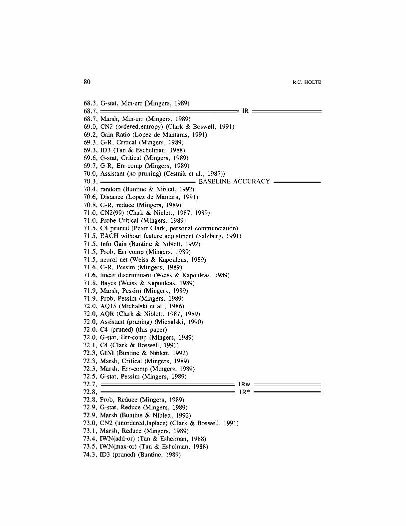
APPENDIX C. Survey of results for each dataset

The results included in this survey were produced under a very wide variety of experimen-tal conditions, and therefore it is impossible to compare them in any detailed manner. Mostof the results are averages over a number of runs, where each run involves splitting thedataset into disjoint training and test sets and using the test set to estimate the accuracyof the rule produced given the training set. But the number of runs varies considerably,as does the ratio of the sizes of the training and test set, and different methods of "ran-domly" splitting have sometimes been used (e.g., cross-validation, stratified sampling, andunstratified sampling). Furthermore, it is virtually certain that some papers reporting resultson a dataset have used slightly different versions of the dataset than others, it being com-mon practice to make "small" changes to a dataset for the purposes of a particularexperiment.

Dataset BC62.0, "B" (Schoenauer & Sebag, 1990)62.0, Assistant (no pruning) (Clark & Niblett, 1987, 1989)65.0, Bayes (Clark & Niblett, 1987, 1989)65.1, CN2 (ordered.laplace) (Clark & Boswell, 1991)65.3, nearest neighbor (Weiss & Kapouleas, 1989)65.6, Bayes(second order) (Weiss & Kapouleas, 1989)65.6, quadratic discriminant (Weiss & Kapouleas, 1989)66.0, AQTT15 (Michalski, 1990)66.3, ID unpruned (Peter Clark, personal communication)66.8, CN2 ordered (Peter Clark, personal communication)66.8, G-R, Min-err (Mingers, 1989)66.9, C4 unpruned (Peter Clark, personal communciation)67.0, Assistant (no pruning) (Michalski, 1990)67.4, Prob, Min-err (Mingers, 1989)68.0, AQ11/15 (Tan & Eshelman, 1988)68.0, AQ15 (Salzberg, 1991)68.0, AQTT15 (biggest disjuncts) (Michalski, 1990)68.0, AQTT15 (unique > 1) (Michalski, 1990)68.0, Assistant (pruning) (Clark & Niblett, 1987, 1989)

80 R.C. HOLTE

68.3, G-stat, Min-err [Mingers, 1989)68.7, IR68.7, Marsh, Min-err (Mingers, 1989)69.0, CN2 (ordered.entropy) (Clark & Boswell, 1991)69.2, Gain Ratio (Lopez de Mantaras, 1991)69.3, G-R, Critical (Mingers, 1989)69.3, ID3 (Tan & Eschelman, 1988)69.6, G-stat, Critical (Mingers, 1989)69.7, G-R, Err-comp (Mingers, 1989)70.0, Assistant (no pruning) (Cestnik et al., 1987))70.3, BASELINE ACCURACY70.4, random (Buntine & Niblett, 1992)70.6, Distance (Lopez de Mantara, 1991)70.8, G-R, reduce (Mingers, 1989)71.0, CN2(99) (Clark & Niblett, 1987, 1989)71.0, Probe Critical (Mingers, 1989)71.5, C4 pruned (Peter Clark, personal communciation)71.5, EACH without feature adjustment (Salzberg, 1991)71.5, Info Gain (Buntine & Niblett, 1992)71.5, Prob, Err-comp (Mingers, 1989)71.5, neural net (Weiss & Kapouleas, 1989)71.6, G-R, Pessim (Mingers, 1989)71.6, linear discriminant (Weiss & Kapouleas, 1989)71.8, Bayes (Weiss & Kapouleas, 1989)71.9, Marsh, Pessim (Mingers, 1989)71.9, Prob, Pessim (Mingers, 1989)72.0, AQ15 (Michalski et al., 1986)72.0, AQR (Clark & Niblett, 1987, 1989)72.0, Assistant (pruning) (Michalski, 1990)72.0, C4 (pruned) (this paper)72.0, G-stat, Err-comp (Mingers, 1989)72.1, C4 (Clark & Boswell, 1991)72.3, GINI (Buntine & Niblett, 1992)72.3, Marsh, Critical (Mingers, 1989)72.3, Marsh, Err-comp (Mingers, 1989)72.5, G-stat, Pessim (Mingers, 1989)72.7, IRw72.8, IR*72.8, Prob, Reduce (Mingers, 1989)72.9, G-stat, Reduce (Mingers, 1989)72.9, Marsh (Buntine & Niblett, 1992)73.0, CN2 (unordered,laplace) (Clark & Boswell, 1991)73.1, Marsh, Reduce (Mingers, 1989)73.4, IWN(add-or) (Tan & Eshelman, 1988)73.5, IWN(max-or) (Tan & Eshelman, 1988)74.3, ID3 (pruned) (Buntine, 1989)


75.0, "C2" (Schoenauer & Sebag, 1990)75.6, Bayes/N (Buntine, 1989)76.1, Bayes (Buntine, 1989)76.2, ID3 (averaged) (Buntine, 1989)77.0, Assistant (pre-pruning) (Cestnik et al., 1987)77.1, CART (Weiss & Kapouleas, 1989)77.1, PVM (Weiss & Kapouleas, 1989)77.6, EACH with feature adjustment (Salzberg, 1991)78.0, "D3" (Schoenauer & Sebag, 1990)78.0, Assistant (post-pruning) (Cestnik et al., 1987)78.0, Bayes (Cestnik et al., 1987)

Dataset CH67.6, 1R68.3, IRw69.2, 1R*85.4, Bayes (Buntine, 1989)91.0, CN2 (Holte et al., 1989)93.9, perceptron (Shavlik et al., 1991)96.3, back propagation (Shavlik et al., 1991)96.4, ID3 (pruned) (Buntine, 1989)96.9, ID3 (unpruned) (Buntine, 1989)97.0, ID3 (Shavlik et al., 1991)99.2, C4 (pruned) (this paper)

Dataset GL45.5, NTgrowth (de la Maza, 1991)46.8, random (Buntine & Niblett, 1992)48.0, Proto-TO (de la Maza, 1991)49.4, Info Gain (Buntine & Niblett, 1992)53.8, 1R56.3, 1R*59.5, Marsh (Buntine & Niblett, 1992)60.0. GINI (Buntine & Niblett. 1992)62.2, IRw63.2, C4 (pruned) (this paper)65.5, C4 (de la Maza, 1991)

Dataset HD60.5, perceptron (Shavlik et al., 1991)70.5, growth (Aha & Kibler, 1989)71.1, K-nearest neighbor growth (K=3) (Aha & Kibler, 1989)71.2, IDS (Savliketal., 1991)71.3, disjunctive spanning (Aha & Kibler, 1989)71.4, growth (Kibler & Aha, 1988)73.4, 1R

82 R.C. HOLTE

73.6, C4 (pruned) (this paper)74.8, C4 (Kibler & Aha, 1988)75.4, C4 (Aha & Kibler, 1989)76.2, proximity (Aha & Kibler, 1989)76.4, IRT (Jensen, 1992)76.6. IRw77.0, NTgrowth (Kibler & Aha, 1988)77.9, NTgrowth (Aha & Kibler, 1989)78.0, 1R*78.7, NT disjunctive spanning (Aha & Kibler, 1989)79.2, K-nearest neighbor (K=3) (Aha & Kibler, 1989)79.4, NT K-nearest neighbor growth (K=3) (Aha & Kibler, 1989)80.6, back propagation (Shavlik et al., 1991)

Dataset HE38.7, NTgrowth (de la Maza, 1991)71.3, CN2 (ordered.entropy) (Clark & Boswell, 1991)76.3, 1R77.6, CN2 (ordered.laplace) (Clark & Boswell, 1991)77.8, ID unpruned (Peter Clark, personal communication)78.6, Gain Ratio (Lopez de Mantaras, 1991)79.3, C4 (Clark & Boswell, 1991)79.3. Distance fLooez de Mantaras. 1991)79.4, BASELINE ACCURACY79.8, C4 (de la Maza, 1991)79.8, m=0.0 (Cestnik & Bratko, 1991)79.8, m=0.01 (Cestnik & Bratko, 1991)79.9, Proto-TO (de la Maza, 1991)80.0, (cited in the UCI files) (Diaconis & Efron, 1983)80.0, Assistant (no pruning) (Cestnik et al., 1987)80.1, CN2 (unordered.laplace) (Clark & Boswell, 1991)81.1, m=l (Cestnik & Bratko, 1991)81.2, C4 (pruned) (this paper)81.5, m=0.5 (Cestnik & Bratko, 1991)82.0, Assistant (post-pruning) (Cestnik et al., 1987)82.1, laplace (Cestnik & Bratko, 1991)83.0, Assistant (pre-pruning) (Cestnik et al., 1987)83.6, m=3 (Cestnik & Bratko, 1991)83.8, m=128 (Cestnik & Bratko, 1991)83.8, m=32 (Cestnik & Bratko, 1991)83.8, m=64 (Cestnik & Bratko, 1991)83.8, m=999 (Cestnik & Bratko, 1991)84.0, Bayes (Cestnik et al., 1987)84.0, m=8 (Cestnik & Bratko, 1991)84.5, IRw


84.5, m=4 (Cestnik & Bratko, 1991)85.5, m=12 (Cestnik & Bratko, 1991)85.5, m=16 (Cestnik & Bratko, 1991)85.8, 1R*

Dataset HY88.4, quadratic discriminant (Weiss & Kapouleas, 1989)92.4, Bayes(second order) (Weiss & Kapouleas, 1989)92.6, random (Buntine & Niblett, 1992)93.9, linear discriminant (Weiss & Kapouleas, 1989)95.3, nearest neighbor (Weiss & Kapouleas, 1989)96.1, Bayes (Weiss & Kapouleas, 1989)97.1, growth (Kibler & Aha, 1988)97.2, 1R97.4, 1R*97.7, NTgrowth (Kibler & Aha, 1988)98.0, IRw98.2, C4 (Kibler & Aha, 1988)98.5, neural net (Weiss & Kapouleas, 1989)98.7, Marsh (Buntine & Niblett, 1992)99.0, GINI (Buntine & Niblett, 1992)99.1, C4 (pruned) (this paper)99.1, Info Gain (Buntine & Niblett, 1992)99.1, PT2 (Utgoff & Brodley, 1990)99.3, C4-rules (Quinlan, 1987)99.3, PVM (Weiss & Kapouleas, 1989)99.4, C4 (Quinlan, 1987)99.4, CART (Weiss & Kapouleas, 1989)99.7, C4 (Quinlan et al., 1986)

Dataset IR84.0, Bayes(second order), (cross-validation) (Weiss & Kapouleas, 1989)85.8, random (Buntine & Niblett, 1992)89.3, Prob, Reduce (Mingers, 1989)90.5, Prob, Err-comp (Mingers, 1989)91.1, Marsh, Critical (Mingers, 1989)91.2, Marsh, Pessim (Mingers, 1989)91.3, Prob, Critical (Mingers, 1989)92.2, Marsh, Min-err (Mingers, 1989)92.3, NTgrowth (de la Maza, 1991)92.4, Marsh, Err-comp (Mingers, 1989)92.4, Marsh, Reduce (Mingers, 1989)92.4, Prob, Pessim (Mingers, 1989)92.4, growth (Kibler & Aha, 1988)92.5, G-R, Critical (Mingers, 1989)92.5, G-R, Err-comp (Mingers, 1989)

84 R.C. HOLTE

92.5, G-R, Pessim (Mingers, 1989)92.5, G-R, reduce (Mingers, 1989)92.6, EACH without feature adjustment (Salzberg, 1991)92.8, G-stat, Critical (Mingers, 1989)92.8, G-stat, Err-comp (Mingers, 1989)92.8, G-stat, Min-err (Mingers, 1989)92.8, G-stat, Pessim (Mingers, 1989)92.8, G-stat, Reduce (Mingers, 1989)93.0, CART (Salzberg, 1991)93.2, G-R, Min-err (Mingers, 1989)93.3, Bayes, (cross-validation) (Weiss & Kapouleas, 1989)93.3, Prob. Min-err (Mingers, 1989)93.5, 1R93.8, C4 (pruned) (this paper)94.0, ID3 (pruned (Buntine, 1989)94.2, C4 (de la Maza, 1991)94.2, ID3 (Catlett, 199la)94.2, ID3 (new version (Catlett, 1991a)94.4, C4 (Kibler &Aha, 1988)94.4, ID3 (averaged) (Buntine, 1989)94.5, Marsh (Buntine & Niblett, 1992)94.7, Dasarathy (Hirsh, 1990)95.0, GINI (Buntine & Niblett, 1992)95.1, Info Gain (Buntine & Niblett, 1992)95.3, CART, (cross-validation) (Weiss & Kapouleas, 1989)95.3, EACH with feature adjustment (Salzberg, 1991)95.4, NTgrowth (Kibler & Aha, 1988)95.5, Bayes (Buntine, 1989)95.5, Bayes/N (Buntine, 1989)95.9, 1R*96.0, IRw96.0, PVM, (cross-validation) (Weiss & Kapouleas, 1989)96.0, Proto-TO (de la Maza, 1991)96.0, nearest neighbor, (cross-validation) (Weiss & Kapouleas, 1989)96.7, IVSM, (Hirsh, 1990)96.7, neural net, (cross-validation) (Weiss & Kapouleas, 1989)97.3, quadratic discriminant, (cross-validation) (Weiss & Kapouleas, 1989)98.0, linear discriminant, (cross-validation) (Weiss & Kapouleas, 1989)

Dataset LA71.5, 1R77.0, 1-nearest neighbor (Bergadano et al., 1992)77.3, C4 (pruned) (this paper)80.0, 5-nearest neighbor (Bergadano et al., 1992)80.0, AQ15 (strict of flexible matching) (Bergadano et al., 1992)


83.0, 3-nearest neighbor (Bergadano et al., 1992)83.0, AQ15 ("top rule" truncation) (Bergadano et al., 1992)83.0, AQ15 (TRUNC-SG,flexible matching) (Bergadano et al., 1992)84.2, IRw86.0, Assistant (with pruning) (Bergadano et al., 1992)87.4, 1R*90.0, AQ15 (TRUNC-SG,deductive matching) (Bergadano et al., 1992)

Dataset LY56.1, m=999 (Cestnik & Bratko, 1991)67.7, random (Buntine & Niblett, 1992)69.1, m=128 (Cestnik & Bratko, 1991)70.7, 1R71.5, CN2 (ordered.entropy) (Clark & Boswell, 1991)74.8, m=64 (Cestnik & Bratko, 1991)75.0, m=16 (Cestnik & Bratko, 1991)75.6, GINI (Buntine & Niblett, 1992)75.7, IRw75.7, Marsh (Buntine & Niblett, 1992)75.9, m=12 (Cestnik & Bratko, 1991)75.9, m=32 (Cestnik & Bratko, 1991)76.0, AQR (Clark & Niblett, 1987, 1989)76.0, Assistant (no pruning) (Cestnik et al., 1987)76.0, Assistant (no pruning) (Michalski, 1990)76.0, Assistant (post-pruning) (Cestnik et al., 1987)76.0, Assistant (pre-pruning) (Cestnik et al., 1987)76.0, Info Gain (Buntine & Niblett, 1992)76.4, C4 (Clark & Boswell, 1991)76.8, m=8 (Cestnik & Bratko, 1991)77.0, Assistant (pruning) (Michalski, 1990)77.1, laplace (Cestnik & Bratko, 1991)77.1, m=4 (Cestnik & Bratko, 1991)77.3, 1R*77.3, m=0.01 (Cestnik & Bratko, 1991)77.3, m=0.5 (Cestnik & Bratko, 1991)77.3, m=l (Cestnik & Bratko, 1991)77.3, m=2 (Cestnik & Bratko, 1991)77.3, m=3 (Cestnik & Bratko, 1991)77.5, C4 (pruned) (this paper)77.5, m=0.0 (Cestnik & Bratko, 1991)78.0, Assistant (pruning) (Clark & Niblett, 1987, 1989)78.4, ID3 (averaged) (Buntine, 1989)79.0, Assistant (no pruning) (Clark & Niblett, 1987, 1989)79.0, Bayes (Cestnik et al., 1987)79.6, CN2 (ordered.laplace) (Clark & Boswell, 1991)

86 R.C. HOLTE

80.0, AQTT15 (unique> 1) (Michalski, 1990)81.0, AQTT15 (Michalski, 1990)81.7, CN2 (unordered.laplace) (Clark & Boswell, 1991)82.0, AQ15 (Michalski et al., 1986)82.0, AQTT15 (biggest disjuncts) (Michalski, 1990)82.0, Bayes/N (Buntine, 1989)82.0, CN2(99) (Clark & Niblett, 1987, 1989)83.0, Bayes (Clark & Niblett, 1987, 1989)85.1, Bayes (Buntine, 1989)

Dataset MU91.2, random (Buntine & Niblett, 1992)92.7, Marsh (Buntine & Niblett, 1992)95.0, HILLARY (Iba et al., 1988)95.0, STAGGER (Schlimmer, 1987)98.4, 1R98.4, 1R*98.5, IRw98.6, GINI (Buntine & Niblett, 1992)98.6, Info Gain (Buntine & Niblett, 1992)99.1, neural net (Yeung, 1991)99.9, ID3, C4 (Wirth & Catlett, 1988)

100.0, C4 (pruned) (this paper)

Dataset SE91.8, growth (Kibbler & Aha, 1988)95.0, 1R95.0, 1R*95.0, IRw95.0, RAF (Quinlan, 1989)95.2, RUU (Quinlan, 1989)95.4, RSS (Quinlan, 1989)95.9, NTgrowth (Kibler & Aha, 1988)96.1, RPF (Quinlan, 1989)96.2, RFF (Quinlan, 1989)96.3, RIF (Quinlan, 1989)96.8, RCF (Quinlan, 1989)97.3, C4 (Kibler & Aha, 1988)97.7, C4 (pruned) (this paper)99.2, C4 (Quinlan et al., 1986)

Dataset VO84.0, 3-nearest neighbor (Bergadano et al., 1992)84.0, 5-nearest neighbor (Bergadano et al., 1992)84.6, random (Buntine & Niblett, 1992)


85.0, AQ15 ("top rule" truncation) (Bergadano et al., 1992)85.2, NT K-nearest neighbor growth (K=3) (Aha & Kibler, 1989)86.0, 1-nearest neighbor (Bergadano et al., 1992)86.0, AQ15 (strict or flexible matching) (Bergadano et al., 1992)86.0, Assistant (with pruning) (Bergadano et al., 1992)86.2, K-nearest neighbor (K=3) (Aha & Kibler, 1989)86.4, K-nearest neighbor growth (K=3) (Aha & Kibler, 1989)88.2, Marsh (Buntine & Niblett, 1992)90.4, Proto-TO (de la Maza, 1991)90.6, NTgrowth (de la Maza, 1991)90.7, growth (Aha & Kibler, 1989)90.8, IWN(add-or) (Tan & Eshelman, 1988)91.7, proximity. (Aha & Kibler, 1989)91.9, NTgrowth (Aha & Kibler, 1989)92.0, AQ15 (TRUNC-SG,deductive matching) (Bergadano et al., 1992)92.0, AQ15 (TRUNC-SG,flexible matching) (Bergadano et al., 1992)92.9, NT disjunctive spanning (Aha & Kibler, 1989)93.6, CN2 (ordered,entropy) (Clark & Boswell, 1991)93.9, IWN(max-or) (Tan & Eshelman, 1988)94.0, ID3 (Fisher & McKusick, 1989)94.3, IWN(add-or) (Tan & Eshelman, 1988)94.5, C4 (Aha & Kibler, 1989)94.8, CN2 (ordered,laplace) (Clark & Boswell, 1991)94.8, CN2 (unordered,laplace) (Clark & Boswell, 1991)95.0, IRT (Jensen, 1991)95.0, STAGGER (Schlimmer, 1987)95.2, 1R95.2, 1R*95.3, C4 (de la Maza, 1991)95.3, neural net (Yeung, 1991)95.4, Info Gain (Buntine & Niblett, 1992)95.5, GINI (Buntine & Niblett, 1992)95.6, IRw95.6, C4 (Clark & Boswell, 1991)95.6, C4 (pruned) (this paper)

Oataset V184.4, random (Buntine & Niblett, 1992)84.9, Marsh (Buntine & Niblett, 1992)86.8, 1R87.0, Info Gain (Buntine & Niblett, 1992)87.2, GINI (Buntine & Niblett, 1992)87.4, IRw87.9, 1R*89.4, C4 (pruned) (this paper)

88 R.C. HOLTE

APPENDIX D. Data from the 25 runs on each dataset.

IR*

Dataset

BCCHGL02HDHEHOHYIRLALYMUSESOvoV1

mean

72.4669.2456.4477.0278.0085.1481.1897.2095.9287.3777.2898.4495.0087.0095.1887.93

std. dev.

4.230.955.063.882.686.231.950.671.554.483.750.200.546.621.522.22

C4

mean

71.9699.1963.1674.2673.6281.2383.6199.1393.7677.2577.52

100.097.6997.5195.5789.36

std. dev.

4.360.275.716.614.445.123.410.272.965.894.460.00.403.941.312.45

IRw

72.7'68.3

62.278.576.5784.581.598.096.084.275.798.595.087.295.687.4

C4-1R*

-0.82134.7

4.98-1.93-5.18-2.69

4.0513.44

-3.61-7.11

0.2137.4730.36.551.593.93

t-values

!R*-lRw

-0.274.85

-5.53-1.90

2.620.51

-0.86-5.88-0.25

3.472.07

-1.440.04

-0.15-1.34

1.17

C4-lRw

-0.83571

0.86-3.17-3.26-3.13

3.0120.59-3.71-5.78

2.0000

32.812.81

-0.123.92

Acknowledgments

This work was supported in part by an operating grant from the Natural Sciences andEngineering Research Council of Canada. I thank Ross Quinlan for providing the sourcefor C4.5 and David Aha for his work in creating and managing the UCI dataset collection.I am greatly indebted to Doug Fisher, Peter Clark, Bruce Porter, and the "explanation"group at the University of Texas at Austin (Ray Mooney, Rich Mallory, Ken Murray, JamesLester, and Liane Acker) for the extensive comments they provided on drafts of this article.Helpful feedback was also given by Wray Buntine and Larry Watanabe.

Notes

1. Conditions under which pruning leads to a decrease in accuracy have been investigated by Schaffer (1992;in press) and Fisher and Schlimmer (1988).

2. Clark and Boswell (1991) offer some discussion of this phenomenon.3. In the version of this dataset in the Irvine collection, this attribute has only 4 values.4. It is not always possible to be certain that a dataset described in the literature is identical to the dataset with

the same name on which 1Rw was measured. The survey includes all results for which there is no evidencethat the datasets differ.

5. HY, SE: Quinlan et al. (1986). LA: Bergadano et al. (1992). MU, VO (V1): Schlimmer (1987).6. HO: McLeish and Cecile (1990). BC, LY: Cestnik et al. (1987). For LY, some grouping of values was done,

as in VO.7. The dynamic complexity of the BC dataset is less than 1 because C4 occasionally produces a decision tree

that consists of nothing but a leaf (all examples are classified the same without testing a single attribute).8. For example, the space shuttle application described in Catlett (1991a).9. A recursive partitioning algorithm similar to Catlett's (1991b) creates partitions that are different than IR's,

and no less accurate.10. 1R produces a rule having three leaves and an accuracy of 95.2%.11. On two datasets Weiss et al. (1990), searched exhaustively through all rules up to a certain length (2 in one

case, 3 in the other). If longer, more accurate rules exist, no one has yet found them.


References

Aha, D.W., & Kibler, D. (1989). Noise-tolerant instance-based learning algorithms. Proceedings of the EleventhInternational Joint Conference on Artificial Intelligence (pp. 794-799). San Mateo, CA: Morgan Kaufmann.

Bergandano, F., Matwin, S., Michalski, R.S., & Zhang, J. (1992). Learning two-tiered descriptions of flexibleconcepts: The Poseidon system. Machine Learning, 8, 5-44.

Buntine, W. (1989). Learning classification rules using Bayes. in A Segre (Ed.), Proceedings of the 6th Inter-national Workshop on Machine Learning (pp. 94-98). San Mateo, CA: Morgan Kaufmann.

Buntine, W., & Niblett, T. (1992). A further comparison of splitting rules for decision-tree induction. MachineLearning, 8, 75-86.

Catlett, J. (1991a). Megainduction: A test flight. In L.A. Birnbaum & G.C. Collins (Eds.), Proceedings of theEighth International Conference on Machine Learning (pp. 596-599). San Mateo, CA: Morgan Kaufmann.

Catlett, J. (1991b). On changing continuous attributes into ordered discrete attributes. In Y. Kodratoff (Ed.),Machine Learning—EWSL-91 (pp: 164-178). Springer-Verlag.

Cestnik, B., & Bratko, I. (1991). On estimating probabilities in tree pruning. In Y. Kodratoff (Ed.) MachineLearning—EWSL-91 (pp. 138-150). Springer-Verlag.

Cestnik, G., Konenenko, I., & Bratko, I. (1987). Assistant-86: A knowledge-elicitation tool for sophisticatedusers. In I. Bratko & N. Lavrac (Eds.), Progress in Machine Learning (pp. 31-45). Wilmslow, England: SigmaPress.

Clark, P., & Boswell, R. (1991). Rule induction with CN2: Some recent improvements. In Y. Kodratoff (Ed.),Machine Learning—EWSL-91 (pp. 151-163). Springer-Verlag.

Clark, P., & Niblett, T. (1989). The CN2 induction algorithm. Machine Learning, 3, 261-283.Clark, P., & Niblett, T. (1987). Induction in noisy domains. In I. Bratko & N. Lavrac (Eds.), Progress in machine

learning (pp. 11-30). Wilmslow, England: Sigma Press,de la Maza, M. (1991). A prototype based symbolic concept learning system. In L.A. Birnbaum & G.C. Collins

(Eds.), Proceedings of the Eighth International Conference on Machine Learning (pp. 41-45). San Mateo,CA: Morgan Kaufmann.

Diaconis, P., & Efron, B. (1983). Computer-intensive methods in statistics. Scientific American, 248.Fisher, D.H. (1987). Knowledge acquisition via incremental conceptual clustering. Machine Learning, 2, 139-172.Fisher, D.H. & McKusick, K.B. (1989). An empirical comparison of ID3 and back-propagation. Proceedings

of the Eleventh International Joint Conference on Artificial Intelligence (pp. 788-793). San Mateo, CA: MorganKaufmann.

Fisher, D.H., & Schlimmer, J.C. (1988). Concept simplification and prediction accuracy. In J. Laird (Ed.), Pro-ceedings of the Fifth International Conference on Machine Learning (pp. 22-28). San Mateo, CA: MorganKaufmann.

Hirsh, H. (1990). Learning from data with bounded inconsistency. In B.W. Porter & R.J. Mooney (Eds.), Pro-ceedings of the Seventh International Conference on Machine Learning (pp. 32-39). San Mateo, CA: MorganKaufmann.

Holder, L.B., Jr., (1991). Maintaining the utility of learned knowledge using model-based adaptive control. Ph.D.thesis, Computer Science Department, University of Illinois at Urbana-Champaign.

Holte, R.C., Acker, L., & Porter, B.W. (1989). Concept learning and the problem of small disjuncts. Proceedingsof the Eleventh International Joint Conference on Artificial Intelligence (pp. 813-818). San Mateo, CA: MorganKaufmann.

Iba, W.F., & Langley, P. (1992). Induction of one-level decision trees. In D. Sleeman & P. Edwards (Eds.) Pro-ceedings of the Ninth International Conference on Machine Learning (pp. 233-240). San Mateo, CA: MorganKaufmann.

Iba, W., Wogulis, J., & Langley, P. (1988). Trading off simplicity and coverage in incremental concept learning.In J. Laird (Ed.), Proceedings of the Fifth International Conference on Machine Learning (pp. 73-79). SanMateo, CA: Morgan Kaufmann.

Jensen, D. (1992). Induction with randomization testing: Decision-oriented analysis of large data sets. Ph.D.thesis, Washington University, St. Louis, Missouri.

Kibler, D., & Aha, D.W. (1988). Comparing instance-averaging with instance-filtering learning algorithms. InD. Sleeman (Ed.), EWSL88: Proceedings of the 3rd European Working Session on Learning (pp. 63-69). Pitman.

Lopez de Mantaras, R. (1991). A Distance-based attribute selection measure for decision tree induction. MachineLearning, 6, 81-92.

90 R.C. HOLTE

McLeish, M., & Cecile, M. (1990). Enhancing medical expert systems with knowledge obtained from statisticaldata. Annals of Mathematics and Artificial Intelligence, 2, 261-276.

Michalski, R.S. (1990). Learning flexible concepts: fundamental ideas and a method based on two-tiered represen-tation. In Y. Kodratoff & R.S. Michalski (Eds.), Machine Learning: An Artificial Intelligence Approach (Vol. 3).San Mateo, CA: Morgan Kaufmann.

Michalski, R.S., & Chilausky, R.L. (1980). Learning by being told and learning from examples: An experimen-tal comparison of the two methods of knowledge acquisition in the context of developing an expert system forsoybean disease diagnosis. International Journal of Policy Analysis and Information Systems, 4(2), 125-161.

Michalski, R.S., Mozetic, I., Hong, J., & Lavrac, N. (1986). The multi-purpose incremental learning systemAQ15 and its testing application to three medical domains. Proceedings of the Fifth National Conference onArtificial Intelligence (pp. 1041-1045). San Mateo, CA: Morgan Kaufmann.

Mingers, J. (1989). An empirical comparison of pruning methods for decision tree induction. Machine Learning,4(2), 227-243.

Quinlan, J.R. (1989). Unknown attribute values in induction. In A. Segre (Ed.), Proceedings of the 6th Inter-national Workshop on Machine Learning (pp. 164-168). San Mateo, CA: Morgan Kaufmann.

Quinlan, J.R. (1987). Generating production rules from decision trees. Proceedings of the Tenth InternationalJoint Conference on Artificial Intelligence (pp. 304-307). San Mateo, CA: Morgan Kaufmann.

Quinlan, J.R. (1986). Induction of decision trees, Machine Learning, 1, 81-106.Quinlan, J.R., Compton, P.J., Horn, K.A., & Lazurus, L. (1986). Inductive knowledge acquisition: a case study.

Proceedings of the Second Australian Conference on Applications of Expert Systems. Sydney, Australia.Rendell, L., & Seshu, R. (1990). Learning hard concepts through constructive induction. Computational In-

telligence, 6, 247-270.Salzberg, S. (1991). A nearest hyperrectangle learning method. Machine Learning, 6, 251-276.Saxena, S. (1989). Evaluating alternative instance representations. In A. Segre (Ed.), Proceedings of the Sixth

International Conference on Machine Learning (pp. 465-468). San Mateo, CA: Morgan Kaufmann.Schaffer, C. (in press). Overfitting avoidance as bias. Machine Learning.Schaffer, C. (1992). Sparse data and the effect of overfitting avoidance in decision tree induction. Proceedings

ofAAAI-92, the Tenth National Conference on Artificial Intelligence.Schlimmer, J.S. (1987). Concept acquisition through representational adjustment (Technical Report 87-19). Ph.D.

thesis, Department of Information and Computer Science, University of California, Irvine.Schoenauer, M., & Sebag, M. (1990). Incremental learning of rules and meta-rules. In B.W. Porter & R.J. Mooney

(Eds.), Proceedings of the Seventh International Conference on Machine Learning (pp. 49-57). San Mateo,CA: Morgan Kaufmann.

Shapiro, A.D. (1987). Structured induction of expert systems. Reading, MA: Addison-Wesley.Shavlik, J., Mooney, R.J., & Towell, G. (1991). Symbolic and neural learning algorithms: An experimental com-

parison. Machine Learning, 6, 111-143.Tan, M., & Eshelman, L. (1988). Using weighted networks to represent classification knowledge in noisy do-

mains. In J. Laird (Ed.), Proceedings of the Fifth International Conference on Machine Learning (pp. 121-134).San Mateo, CA: Morgan Kaufmann.

Tan, M., & Schlimmer, J. (1990). Two case studies in cost-sensitive concept acquisition. Proceedings of AAAI-90,the Eighth National Conference on Artificial Intelligence (pp. 854-860). Cambridge, MA: MIT Press.

Utgoff, P.E., & Bradley, C.E. (1990). An incremental method for finding multivariate splits for decision trees.In B.W. Porter & R.J. Mooney (Eds.), Proceedings of the Seventh International Conference on Machine Learn-ing (pp. 58-65). San Mateo, CA: Morgan Kaufmann.

Weiss, S.M., Galen, R.S., & Tadepalli, P.V. (1990). Maximizing the predictive value of production rules. Arti-ficial Intelligence, 45, 47-71.

Weiss, S.M., & Kapouleas, I. (1990). An empirical comparison of pattern recognition, neural nets, and machinelearning classification methods. Proceedings of the Eleventh International Joint Conference on Artificial Intel-ligence (pp. 781-787). San Mateo, CA: Morgan Kaufmann.

Wirth, J., & Catlett, J. (1988). Experiments on the costs and benefits of windowing in IDS. In J. Laird (Ed.),Proceedings of the Fifth International Conference on Machine Learning (pp. 87-99). San Mateo, CA: MorganKaufmann.

Yeung, D.-Y. (1991). A neural network approach to constructive induction. In L.A. Birnbaum & G.C. Collins(Eds.), Proceedings of the Eighth International Conference on Machine Learning (pp. 228-232). San Mateo,CA: Morgan Kaufmann.

Received April 22, 1991Accepted July 17, 1992Final Manuscript September 10, 1992

Very Simple Classification Rules Perform Well on Most ...

Documents

Transcript of Very Simple Classification Rules Perform Well on Most ...