NASA Contractor Report 3096

Vertical Motions in the Equatorial Middle Atmosphere

M. L. Weisman

CONTRACT NASG-2726 APRIL 1979

TECH LIBRARY KAFB, NM

llillllllllllldlRMlIll~ 00bLB78

NASA Contractor Report 3096

Vertical Motions in the Equatorial Middle Atmosphere

M. L. Weisman The Pennsylvania State University University Park, Pennsylvania

Prepared for Wallops Flight Center under Contract NASG-2726

National Aeronautics and Space Administration

Scientific and Technical Information Office

1979

TABLE OF CONTENTS

ABSTRACT ..........................

LIST OF FIGURES ......................

LIST OF TABLES .......................

LIST OF SYMBOLS ......................

ACKNOWLEDGEMENTS ......................

1.0

2.0

3.0

4.0

5.0

INTRODUCTION 1.1 Importance of Vertical Motions ........ 1.2 Vertical Velocities and the Equations of

Motion .................... 1.3 Vertical Motion Studies in the Middle

Atmosphere .................. 1.4 The Diurnal Experiment and Equatorial Vertical

Motions ....................

1 2

5

12

16

DERIVATION OF THE VERTICAL VELOCITY EQUATION .... 2.1 A Generalized Thermodynamic Vertical Velocity

Equation ................... 2.2 Diabatic Processes .............. 2.3 Scale Analysis and the Final Equation .....

23

23 27 32

VERTICAL VELOCITY ANALYSIS ............. 39 3.1 Calculation Scheme .............. 39 3.2 Verification Scheme .............. 47

RESULTS AND DISCUSSION ............... 53 4.1 Time Series Cross Sectional Analysis ..... 53 4.2 Internal Consistency ............. 68 4.3 Comparison with Atmospheric Wave Theory .... 76

SUMMARY, CONCLUSIONS, AND RECOMMENDATIONS FOR FUTUREWORK.. ................... 92

96

98

101

104

106

110

APPENDIX A: APPROXIMATION OF & (- $ VHp) TERM ......

APPENDIX B: SCALING ....................

APPENDIX C: ERROR ESTIMATES ................

APPENDIX D: 312 CURVE ..................

APPENDIX E: FOURIER ANALYSIS ...............

REFERENCES.. .......................

Page

iii

vi

viii

ix

xi

iii

LIST OF FIGURES

Page Figure

1

2A

2B

2c

3A

3B

4A

4B

7A

7B

8A

SB

9A

9B

Diurnal experiment stations, Xarch 19-20. 1974. . . 17

Perturbations in zonal winds at Kourou. March 19-20, 1974 . . . . . . . . . . . . . . . . . 19

Perturbations in meridional winds at Kourou. March 19-20. 1974 . . . . . . . . . . . . . . . . . 20

Perturbations in temperatures at Kourou, March 19-20. 1974 . . . . . . . . . . . . . . . . . 21

Net radiative heating over diurnal period for equatorial regions (solstice) . . . . . . . . . . . 30

Temperature change caused by solar radiation over a diurnal period for equatorial regions . . . 30

Time dependence of proposed diabatic function . . . 31

Height dependence of proposed diabatic function . . 31

Finite differencing errors for derivative approximation . . . . . . . . . . . . . . . . . . . 42

Finite difference schemes: Dots represent data points, >i represents assigned position of calculated quantities, \ represents assigned position of calculated quantities on the boundary. . . . . . . . . . . . . . . . . . . . . . 45

Vertical velocities and error estimates for Kourou, scheme A (cm/set) . . . . . . . . . . . . . 57

Vertical velocities and error estimates for Kourou, scheme B (cm/set) . . . . . . . . . . . . . 58

Vertical velocities and error estimates for Ascension Island. scheme A (cm/set> . . . . . . . . 59

Vertical velocities and error estimates for Ascension Island. scheme B (cm/set) . . . . . . . . 60

Vertical velocities and error estimates for Ft. Sherman, scheme A (cm/set). . . . . . . . . . . . . 61

Vertical velocities and error estimates for Ft. Sherman, scheme i? (cm/set). . . . . . . . . . . . . 62

iv

LIST OF FIGURES (Continued)

Figure

10A

10B

11A

11B

12A

12B

13A

13B

14

15

16

17

18

19

Page

Vertical velocities and error estimates for Antigua, scheme A (cm/set) . . . . . . . . . . . . . . . . . 63

Vertical velocities and error estimates for Antigua, scheme B (cm/set) . . . . . . . . . . . . . . . 1 . 64

Vertical velocities and error estimates for Natal, scheme A (cm/set) . . . . . . . . . . . . . . . . .

Vertical velocities and error estimates for Natal, scheme B (cm/set) . . . . . . . . . . . . . . . . .

Vertical velocities and error estimates for Kourou, OOOOZ data left out, scheme A (cm/set) . .

Vertical velocities and error estimates for Kourou. OOOOZ data left out, scheme B (cm/set) . .

Vertical velocities for Kourou as calculated with only local temperature change term, scheme A (cm/set). . . . . . . . . . . . . . . . . . . . . .

Vertical velocities for Kourou as calculated with only local temperature change term, scheme B (cm/set). . . . . . . . . . . . . . . . . . . . . .

Maximum magnitude of vertical velocity at Kourou, Ft. Sherman, and Ascension . . . . . . . . . . . .

Maximum magnitude of vertical velocity at Natal and Antigua . . . . . . . . . . . . . . . . . . . .

Amplitude of diurnal component of vertical velocity at Kourou and Ft. Sherman . . . . . . . .

Amplitude of semidiurnal component of vertical velocity at Kourou and Ft. Sherman . . . . . . . .

Spectral estimates per vertical wavelength . . . .

Phase (hour of maximum) of the diurnal component of vertical velocity at Kourou, Ft. Sherman, and Ascension . . . . . . . . . . . . . . . . . . . . .

65

66

69

70

77

78

80

81

85

86

88

90

V

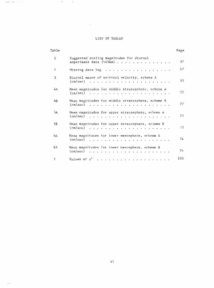
LIST OF TABLES

Table Page

Suggested scaling magnitudes for diurnal experiment data (x45km) . . . . . . . . . . . . . .

2

3

4A

4B

5A

5B

6~

6B

7

Missing data log . . . . . . . . . . . . . . . . .

Diurnal means of vertical velocity. scheme A (cm/set) . . . . . . . . . . . . . . . . . . . . .

Mean magnitudes for middle stratosphere, scheme A (cm/set) . . . . . . . . . . . . . . . . . . . . .

Mean magnitudes for middle stratosphere, scheme B (cm/set) . . . . . . . . . . . . . . . . . . . . .

Mean magnitudes for upper stratosphere, scheme A (cm/set) . . . . . . . . . . . . . . . . . . . . .

Mean magnitudes for upper stratosphere, scheme B (cm/set) . . . . . . . . . . . . . . . . . . . . .

Mean magnitudes for lower mesosphere, scileme A (cm/set> . . . . . . . . . . . . . . . . . . . . .

Mean magnitudes for lower mesosphere, scheme B (cm/set) . . . . . . . . . . . . . . . . . . . . .

Valuesofp' . . . . . . . . . . . . . . . . . . .

37

47

55

72

72

73

73

74

74

103

vi

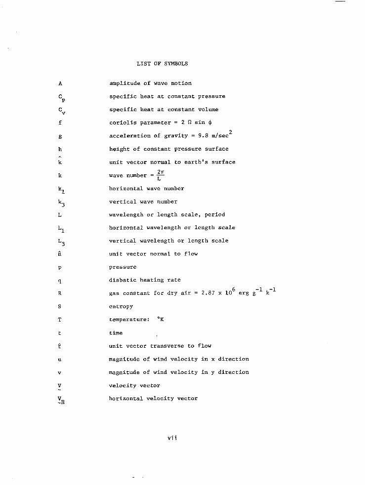
LIST OF SYMBOLS

A

C P

cv

f

g

h A k

k

kl k3 L

P

4

R

S

T

t

t

u

V

V

YH

amplitude of wave motion

specific heat at constant pressure

specific heat at constant volume

coriolis parameter = 2 R sin 4

acceleration of gravity = 9.8 m/set 2

height of constant pressure surface

unit vector normal to earth's surface

wave number = z L horizontal wave number

vertical wave number

wavelength or length scale, period

horizontal wavelength or length scale

vertical wavelength or length scale

unit vector normal to flow

pressure

diabatic heating rate

gas constant for dry air = 2.87 x lo6 erg g -1 k-l

entropy

temperature: "K

time ,

unit vector transverse to flow

magnitude of wind velocity in x direction

magnitude of wind velocity in y direction

velocity vector

horizontal velocity vector

vii

LIST OF SYMBOLS (Continued)

vH W

"P X

Y

2

Y

'Ad

A( 1

6( 1

vH V

P Tr

P

T

w

w g

<P J( >

(‘)

magnitude of horizontal velocity vector

magnitude of vertical velocity vector

a! ' dt

position coordinate in east-west direction

position coordinate in north-south direction

position coordinate normal to earth's surface

1 specific volume - - P

lapse rate f - g

ii adiabatic lapse rate E C P

finite differencing interval; scaling amplitude for derivatives

magnitude of error estimate

gradient, divergence operator on constant height surface

gradient, divergence operator on constant pressure surface

= 3.14159...

density

wave period or time scale

latitude

angular velocity of earth's rotation = 7.292 x 10-5/sec

frequency = $

Brunt V;iisal'a. frequency

relative vorticity in isobaric coordinates

Jacobian Operator

=$o

viii

ACKNOWLEDGKENTS

The author would like to extend his sincere appreciation to

Dr. John J. Oliver0 for the inspiration, guidance, and constructive

criticism that he was always willing to provide. Thanks are also due

to Dr. John H. E. Clark and Dr. John D. Lee for the many helpful dis-

cussions throughout the progress of this work. Additional thanks are

due to Dr. John H. E. Clark for reviewing this manuscript.

Financial support and rocket data has been provided by NASA -

Wallops Flight Center, Virginia under NASA Contract NAS6-2726.

ix

1.0 INTRODUCTION

Throughout the history of meteorology, the atmosphere has been

subdivided into various regions depending on the thought and obser-

vations of the times. These subdivisions have been based both on

actual scientific properties (as in the troposphere, stratosphere, and

mesosphere classifications) or merely on the proximity to man's

influence or direct experience (such as the lower atmosphere, includ-

ing the troposphere, and the upper atmosphere, including everything

above the troposphere). The present is no exception for in the wake

of new public and scientific concern over man's possible impact on

the upper atmosphere, a new subdivision, the "middle atmosphere",

has come into existence. This region includes the stratosphere and

mesosphere (15-85 km in altitude) and is where ozone forms an impor-

tant link between solar radiation and atmospheric dynamics. At the

same time, it is a region relatively void of observations either of

the ground based or satellite type, making all forms of analysis

quite difficult.

The current study is concerned with an important but often times

neglected part of the dynamics in the middle atmosphere, namely,

vertical motions. Observational studies of vertical motions in this

region are virtually non-existent yet observational studies of other

parameters show many discrepencies with theory which point increas-

ingly towards vertical motions as the chief culprit. Unfortunately,

vertical motions cannot be measured directly and while they can be

derived indirectly from other observed quantities, such techniques

are subject to many restrictions which are especially evident in the

L-

middle atmosphere. The goal of the present study is to d.evise a

vertical velocity calculation and analysis scheme consistent with the

middle atmospheric restrictions and apply this technique to an actual

data set. The data to be used for this purpose was obtained from the

Diurnal Experiment of March 19, 20, 1974 and covers equatorial

regions. Before getting into the particulars of this experiment,

however, it will be useful to review the concept of vertical motions

in general and their relationship to current research efforts in the

middle atmosphere.

1.1 IMPORTANCE OF VERTICAL MOTIONS

When one is first introduced to vertical motions in the atmo-

sphere, it is usually in reference to tropospheric weather. Here, it

is found that upward motion produces clouds and precipitation while

downward motion produces clearer, drier weather. Researchers think

of this in terms of vertical transports of moisture, heat. and momen-

tum or as conversion processes in energetic studies, but however it

is viewed, knowledge of the vertical component of the wind is essential

to the understanding of tropospheric circulation. For this reason,

tropospheric vertical motions have been the subject of many research

efforts.

This important role of vertical motions does not stop at the

tropopause, but until recently, studies of the vertical component of

the wind above this level have been virtually nonexistent. To a

large degree, this can be attributed to the lack of observational

data from which such studies could be made, but to some degree, this

2

must also be attributed to the lack of understanding and concern of

processes occurring above the tropopause. As an example, one inform-

ally accepted axiom of the recent past stated that the stratosphere

was too stable to support significant vertical velocities and any-

thing which occurred above the stratosphere was unimportant anyways.

Over the past decade, however, scientific interest in the middle

atmosphere has increased dramatically, this in the wake of greatly

improved observational networks as well as new understanding into

the possible interactions between this region of the atmosphere and

the more familiar troposphere. Indeed, one finds many of the same

large and small scale features previously studied in the troposphere

and along with these features come the same important questions con-

cerning the vertical motions. In addition, many other interesting

processes and phenomena are being isolated and studied which either

are not found in the troposphere or only become significant above the

troposphere. Some of these include sudden stratospheric warmings,

quasibiennial oscillations, atmospheric tides and other forms of

internal gravity waves, ozone and other minor constituent transport,

and radiative transfer. While vertical motions are important in all

of the above processes, particular attention will now be drawn towards

the transport and radiative transfer problems.

Much of the new found interest in the middle atmosphere has been

related in one form or another to the well publicized ozone problem.

While only a minor atmospheric constituent, ozone essentially controls

the dynamics of much of the stratosphere and mesosphere. Its absorp-

tion of ultraviolet radiation supplies much of the forcing for the

atmospheric tides and at the same time shields the surface from

3

these potentially damaging rays. Recent concern has been that man is

in the process of or, in fact, already has adversely affected the

fragile balance which exists between ozone and the various other

atmospheric constituents. Unfortunately, due to the lack of compre-

hensive observations covering many years, significant conclusions can-

not yet be drawn as to the existence of such effects.

One of the major stumbling blocks to the type of scientific

research which could solve this problem has been the lack of knowledge

concerning the transport properties affecting the various trace.con-

stituents which make up the middle atmosphere. Although man's direct

impact on the atmosphere occurs mainly in the troposphere, much of

the attention has been on how the various chemical species are trans-

ported up to or down from the middle atmosphere. Without knowledge

of the vertical motion field, the vertical transport must be approxi-

mated using parameterization schemes and so far, this approach has

produced unsatisfactory and inconsistent results. Being able to

characterize the vertical motion field in the middle atmosphere would

be a vital step towards improving the above schemes and eventually

solving the vertical transport problem.

Another aspect of middle atmospheric research which has received

much attention recently has been the attempt to understand the in-

herent temperature structure of this region and its variations in

space and time. To date, many results have been obtained by assuming

that the observed temperature structure was a direct consequence of

radiative transfer processes or even a state of radiative equilibrium.

Under such an assumption, the observed temperatures could be used to

calculate diabatic heating and cooling rates which would account for

4

the observed temperatures. This, in turn, would help determine the

quantities of the various constituents taking part in the radiative

process. The major drawback is that such an approach ignores horizon-

tal advection of temperature or the adiabatic heating or cooling which

accompanies vertical motions. Indeed, it has been noted over the past

decade or so that vertical profiles and time cross sections of temper-

ature for the middle atmosphere are full of "wiggles" which cannot be

explained via radiative transfer or horizontal advection arguments.

Another possibility is that the observed temperature structure is

being significantly affected by vertical motions. Thus, knowledge

of the vertical motion field would also be an important step towards

understanding the radiative processes of the middle atmosphere.

Unfortunately, the determination of vertical motions is at best

a difficult task. The problem is that their magnitude, usually only

a few cm/set, is too small to be measured directly. They must there-

fore be determined indirectly via the equations of motion. Several

techniques are available for this purpose, but the limited data

availability in the middle atmosphere puts restrictions even on the

use of these methods. The role of vertical motions in the equations

of motion, vertical velocity equations, and these restrictions will

all be discussed in the next section.

1.2 VERTICAL VELOCITIES AND THE EQUATIONS OF MOTION

The most logical starting point for a discussion of vertical

motions in the atmosphere is the complete set of meteorological

equations given below (following Dutton, 1976).

5

?!H at + v l VVH = - + vHp + 2R x YH

dw z=

13? -paZsg

(j dTsaAPzq P dt dt

p = oRT .

(1.1)

(1.2)

(1.3)

(1.4)

(1.5)

These represent the horizontal equation of motion, vertical equation

of motion, first law of thermodynamics, equation of continuity, and

the equation of state respectively. For most research applications,

however, one finds that the acceleration term in equation (1.2) is

much smaller than the remaining terms. Thus, equation (1.2) is

usually replaced by the hydrostatic approximation:

ap -=- a2 Pg * (1.6)

This has the effect of eliminating a prognostic statement for w from

the above system of equations. The vertical velocity must therefore

be determined'diagnostically through the remaining equations. Several

standard techniques have been developed for this purpose, each one

stressing different aspects of the link between vertical motions and

the general circulation. These are briefly described below.

P

6

I. m . ,a . . ._.. . _..__ -_-.-.

The link between the vertical motion field and the horizontal

components of the wind can be expressed via the equation of mass con-

tinuity, equation (1.4). For this purpose, it is more convenient to

use the isobaric form as in Dutton (1976).

V .v+awp=o P - ap

where w 42 = dt is related to w as follows:

P

wP - - pgw .

(l-7)

(1.8)

Upon solving equation (1.7) for w P'

one obtains:

(1.9)

where w

PO

represents the surface value, usually taken to be 0. The

above relation suggests that net horizontal divergence in a column

will lead to negative vertical velocities at the top of the column

while net horizontal convergence will lead to positive vertical

velocities. Equation (1.9) is cormnonly referred to as the kinematic

vertical velocity equation and produces vertical motions which will

ensure that mass is being conserved in the atmosphere.

A second diagnostic equation can be derived from the first law of

thermodynamics, equation 1.3. Upon expanding the time derivatives

and making a few more approximations appropriate to atmospheric con-

ditions, one obtains the following expression (see Chapter 2):

7

-.. ..--_ - -.-_.--.._.._. .- .._.. .,. -... -...._.. ,m .._.. ..- m-,-m. ~-..--....-1.,...11,, I.,, ,,,,,,,,, I ,,,,.,., I I I...,.. ,111 L!Lll, I I II 111.11

I

~+V=V,T+ w= P

(Y - YAd' * (1.10)

The equation demonstrates how the vertical motion field is linked to

the temperature and heating fields. Since the stability term,

(Y - YAd), is usually negative under normal atmospheric conditions,

one can see that local cooling, warm advection, and a positive

diabatic heating rate all contribute positively to the vertical

velocity as estimated by the above expression. Likewise, local

heating, cold advection, and diabatic cooling contribute negatively in

the above expression. If one neglects the diabatic heating term, then

the above expression becomes the standard adiabatic vertical velocity

equation.

Thus, vertical motions in the atmosphere are restricted by both

the conditions of mass continuity and energy conservation. Both of

these conditions along with the hydrostatic approximation can be in-

cluded in one equation first derived by L. F. Richardson (Dutton,

1976):

w=

- !!H

8

(1.11)

One will note, however, that this

difficult to evaluate numerically

Another expression for w can

vorticity equation along with the

1976).

l- W

expression would be much more

then the 'two previous techniques.

be derived using the isobaric

equation of continuity (Dutton,

1 PO

wP = (5, + f) (5, + flP 0

I P

+ 1

(5, + f> 2(&+v= VP') (E,, + f) dp' 1 (1.12)

ll =0 -I

Even though many terms had to be neglected to obtain the above form,

it does portray one of the more useful properties of atmospheric

motion, namely, that fields of vorticity can be directly related to

fields of vertical motion. For forecasters, the above relation

translates into the well known saying that an increase in vorticity

advection with height leads to positive vertical velocities and vice

versa. One could likewise make the statement that vertical motions

tend to develop rotation in an otherwise smooth flow leading to the

cyclones and anticyclones, troughs and ridges found on all synoptic

maps.

Finally, using the complete set of meteorological equations along

with the geostrophic approximation, one can derive the well known

Omega Equation (Dutton, 1976).

VP2 (wpd + 5 (Vp2h + 6) - wpvp2 3 aP2

- $ (Vpwp - VP g > = 2 vp2Jh e)

+ a J(h, ap f VP;;'+ f) - y& VP2 (9, fh) .

P (1.13)

In principle, one could solve this expression for the vertical motion

field, but this would imply using many approximate numerical schemes

which could potentially induce much error into the results. For this

reason, the omega equation is not commonly used in observational

studies of vertical motions but rather is used along with the tendency

equation for numerical weather prediction studies.

The critical factor in determining which if any of equations

(1.9) through (1.l3) can be used to study vertical motions for a

particular case is obviously the data availability. In tropospheric

studies, data is abundant enough to specify horizontal grids of data

points, appropriate boundary conditions, and even local time deriva-

tives so that any of the above techniques can be used. In high

latitude regions of the lower stratosphere, this is still somewhat

the case but for the mid-stratosphere and higher, one usually has only

a handful of stations per hemisphere taking the required observations.

This makes the formation of a horizontal grid of data points a diffi-

cult if not impossible task. For middle and high latitude regions

this problem is alleviated somewhat by the 5, 2, 1, and 0.4 mb synop-

tic charts prepared weekly by the Upper Air branch of the National

Weather Service, but such information is not regularly available for

10

time periods less than a week and even if available, gives virtually

no information concerning features in low latitude or equatorial

regions. With the utility of the above techniques depending on the

availability of horizontal grids of data, it initially appears unfea-

sible to calculate vertical velocities for short time scales and/or

low latitudes in the middle atmosphere.

There is a way around this restriction, however, for through the

use of the geostrophic approximation, one can derive a thermal wind

relation which relates the horizontal advection of temperature to the

vertical shear of the geostrophic wind. This relation can he used in

equation (1.10) to create a single station technique for calculating

vertical velocities.

av g+pxg-F

w= P (Y - YAd> -

(1.14)

Assuming one has a series of observations so that the local change of

temperature term could be evaluated, equation (1.14) can be used with

a single station supplied data set. Considering the potential data

sparsity in the middle atmosphere, the above equation becomes a

prime candidate for use in studying vertical motions in this region.

One important question which must be considered in using any of

the above techniques is how one goes about verifying the results.

The most obvious approach would be to compare the calculations to

actually measured vertical velocities, but as has been previously

suggested, vertical motions cannot be measured directly. One can get

around this difficulty in the troposphere as vertical motions can be

11

correlated quite well with cloud and precipitation patterns. Through

such studies, it has been determined that all of the above techniques

can estimate the sign and order of magnitude of the vertical motions

quite well. Unfortunately, no such correlation procedure exists for

middle atmospheric regions. Thus when working in the middle atmo-

sphere, one must either rely on the results obtained in the troposphere

and assume the same for higher altitudes or one must rely on more

indirect verification procedures. Such procedures will be discussed

in Chapter 3.

By reviewing the equations of motion, we have seen how vertical

motions link the many atmospheric variables together and have seen

that several techniques are available for the actual calculation and

study of vertical motions. In the next section, the focus will

shift specifically to the middle atmosphere, considering in more detail

the data limitations of this region as well as the results of vertical

motion studies in this region to date.

1.3 VERTICAL MOTION STUDIES IN THE MIDDLE ATMOSPHERE

Over the years, observational studies of the stratosphere and

mesosphere have been limited greatly by both the difficulty and

expense of obtaining data from these regions. The relatively inex-

pensive balloon techniques used in the troposphere will supply data

only as high as 25 or 30 km. To obtain observations higher than this,

one must employ meteorological rockets. The Meteorological Rocket

Network (MRN) encompasses only a handful of stations over the entire

northern hemisphere, many of which are in middle and high latitude

12

regions. Except for special experiments, observations of wind and

temperature are usually taken no more frequently than once a week,

and sometimes even less. Once the observations have been taken, they

must be subjected to correction and reduction procedures before the

data can be used. Many times, these procedures differ from station

to station producing very incoherent data sets.

In recent years, the data base has been enhanced somewhat by

satellite derived thickness fields. With the help of this additional

information, weekly northern hemispheric synoptic analysis are now

produced for the 5, 2, 1, and 0.4 mb pressure levels by the Upper Air

Branch of the National Weather Service. These maps depict features

up to about wave number 10 for high latitude regions but still give

virtually no information concerning features in the equatorial

regions. Because of these restrictions, observational studies in the

middle atmosphere have generally been limited to the middle and high

latitudes and to large time and space scales. Thus, the majority of

the research has been on middle and high latitude planetary waves.

One particular feature which has gained much attention recently

has been the sudden stratospheric warmings which characterize many

high latitude winters. These, along with the regular planetary waves,

were the subject of several vertical motion studies during the mid

60's and early 70's. Because of the data limitations, all of these

studies made use of the thermodynamic vertical velocity equation,

either in the form of equation (1.10) or equation (1.14).

Kays and Craig (1965) used equation (1.14) to estimate the

vertical motion field between 26 and 42 km for many of the middle and

high latitude stations of the MRN. As far as is known, this was the

13

first attempt at applying the thermodynamic method above the 10 mb

level (roughly, 31 km). Their results suggested large scale vertical

motions ranging from a few mmjsec during the summer to a few cm/set

during the winter. Both the sign and magnitude of these results were

found to rely on the horizontal advection of temperature term.

Equation (1.14) was used in another study by Quiroz (1969), this

time to study the vertical motion field associated with a major

stratospheric warming event. These calculations ranged between 20

and 44 km in height and again were limited to middle and high latitude

regions. The magnitudes suggested, however, were much larger than the

previous study, ranging up to 60 cmlsec.

Miller (1970) calculated vertical velocities using equation (1.10)

directly. In order to form the necessary horizontal grid of data

points, he made use of the stratospheric height fields described

above. The calculations ran in latitude from 25"N to 65ON in the

western hemisphere and suggested vertical motions on the order of 3-9

cm/set. As with Kays and Craig, Miller found that the sign and order

of magnitude of the derived vertical motions was essentially deter-

mined by the horizontal advection of temperature term.

The important observation which was drawn from these studies,

however, was that the results were consistent with our knowledge of

large scale synoptics and dynamics in this region. This implied that

the thermodynamic technique could be used in middle and high latitudes

to determine at least the sign and order of magnitude of large scale

vertical motions for the middle atmosphere. This result can now be

used as a stepping stone from which to attack the problem of concern

14

in this thesis, namely, the study of vertical motions in the equato-

rial middle atmosphere.

Observational studies in the equatorial middle atmosphere have

been even more limited than for the higher latitudes. Due to the

scarcity of data sets from which proper analysis could be made,

theoretical results seem to be more abundant than observational

results. Much attention has been devoted to studying large time and

space scale features such as Kelvin waves, Rossby-gravity waves, and

the quasibiennial oscillation. Theoretical results, however, suggest

that small time scale features become quite significant in this

region, taking the form of tidal motions and internal gravity waves.

Several special data sets have been obtained for the purpose of

studying these features, especially the tidal motions, but to date,

no results have been presented for vertical motions. One reason for

this has been the lack of sufficient data from which such calculations

could be made, but perhaps just as importantly, working in the vicinity

of the equator puts an additional restriction on the use of equation

(1.14). With the loss of geostrophy near the equator, one apparently

loses the single station technique for calculating the vertical

motions.

A special Diurnal Experiment has solved at least the data aspects

of the above problem. This data set and the additional restriction

of the use of equation (1.14) will be the topic of discussion in the

next section.

15

1.4 THE DIURNAL EXPERIMENT AND EQUATORIAL VERTICAL MOTIONS

In 1974, NASA attempted to obtain a more comprehensive equatorial

data set by organizing and running the Diurnal Experiment. This ex-

periment covered the equinoctial period of March 19, 20 and consisted

of a series of measurements of both horizontal winds and temperatures

taken roughly every three hours for an entire diurnal period. The

observations were taken through the use of meteorological sounding

rockets and reduced values were obtained at 1 km intervals within the

altitude range of 25 to 65 km. In all, eight stations were involved

in the experiment, five of which were located in the vicinity of the

equator (see figure 1). The stations of interest in this particular

study are Kourou (French Guiana), Fort Sherman (Panama Canal Zone),

Ascension Island, Antigua (British West Indies), and Natal (Brazil).

Besides being the most extensive data set ever compiled for

studying short time scale motions in this region, the Diurnal Ex-

periment was unique in many other ways. Not only did each station

use the same measuring device, the Datasonde, but all the data was

subjected to the same correction and reduction procedure. This led

to an unusually coherent data set for studying the middle atmosphere.

The size of the present data set limits the range of time scales

which can be studied from several hours to one day. But fortunately,

theory suggests that these are the scales which should dominate the

motion in this region, taking the form of tidal and other internal

gravity waves. One would thus expect evidence of these waves in the

observed temperature and wind fields. To see that this is the case,

time series cross sections of zonal and meridional winds and

16

0" 1

Fort Church

O0 (9.3N, 8O.OW)

3o"

FIGURE 1. Diurnal Experiment Stations, March 19, 20, 1974.

17

temperature for Kourou are presented in figures 2A, 2B, and 2C.

Perturbations about the diurnal mean are used here to properly depict

the possible wave type features. Regions of positive perturbations

have been shaded in. One will note that continuous features of

diurnal period and less are evident in both the wind and temperature

cross sections with even a tendency to-wards a downward phase progres-

sion. It also appears as if the amplitudes of the variations increases

steadily with height.

All of the above mentioned features are characteristics of tidal

type motions and the results for Kourou are quite representative of

the other stations as well. Schmidlin (1976) and Kao and Lordi

(1977) analyzed the horizontal winds and temperatures for this data

set in an attempt to discern the amplitudes and phases of the various

tidal components. Their results suggested that tidal motions were in-

deed the major contributor to the features evident in the above cross

sections.

The question which is now posed in this thesis is whether the

above data set can be used to calculate and analyse vertical motions

in the equatorial middle atmosphere. We have already seen that several

techniques are available for this purpose but we have also noted that

the data limitations of this region restrict one to using a single

station calculation scheme. One such scheme is available as in

equation (1.14) but this relies on the use of the geostrophic approxi-

mation which does not necessarily hold in equatorial regions. The

first task of this study will thus be to derive a single station verti-

cal velocity calculation scheme which can be used with an equatorial

data set. Perhaps fortuitously, it will be shown in Chapter 2 that

18

I I I I I I I I I I 1 -3.8 -2.3 -9.0 -3.0 60 t

55 -

50 -

s45 - 5

k 2 i_ w I I-

40 '-

35 -

30 -

-I.”

-7.8 -2.3 -0. tll -8.8 -3.3

n I n I) -2.3 E>

-6.0 -

-“.” .L.Y -.- -n L -n h -1.6 -3.1 -0.9

-2.1 -3.1 -1.6 -1.9 -1.9 -2.9 -1.8 -1.3 -4.1

n '1 -7 7 -L 7

25 t I I I I I I I I I

1500 1800 2100 0000 0300 0600 0900 1200 1500

TIME (GMT)

-

FIGURE 2A. perturbations in zonal winds at Kourou, March 19-20, 1974.

60 -

55 -

50 -

345 - l- G Y

40 -

35 -

30 -

-3.3 -3.6 -4.8

LO.6 -12.6 -5.6 ' -10.2 -14.4 -5.9 F

A -6.9 -12.7 -7.1 &l -10.9 -9.4 -5.9 't

-6.8 -10.0 -10.0 -i -7.1 -11.8 -c

-2.4 -1.6 F

25 I I I I I I I I I 1500 1800 2100 0000 0300 0600 0900 1200 1500

TIME (GMT)

FIGURE 2B. Perturbations in meridional winds at Kourou, March 19-20, 1974.

ho -

55 -

50 -

2 x45 -

!E !2 Y

40 -

35 -

30 -

25 -

-4.3 -4.2 -3.2 -2.4 -2.3 -1.6 -1.0 -0.9 -0.8

-7.1 Y-4.6

-6.7 -2.4 -6.5 -4.3 -6.1 -4.3

-1.7 -0.2 -1.0 -2.7 -4.2

-1.6 -2.0 -2.1 -3.0 -4.2 -4.5

m -0.6 -4.3 u

1500 1800 2100 0000 0300 0600 0900 1200 1500 TIME (GRIT)

FIGURE 2C. Perturbations in temperatures at Kourou, March 19-20, 1974.

such a scheme can be derived for the scales of motion depicted in the

Diurnal Experiment data set.

The second task of the study will be to devise an analysis scheme

by which the results can properly be judged. As will be discussed in

Chapter 3, this entails considering the potential numerical error and

numerical stability of the results as well as comparing the results

to the predictions of atmospheric wave theory. In particular, refer-

ence will be made to the theoretical calculations for atmospheric tides

presented by Lindzen (1967), Chapman and Lindzen (1970), and Lindzen

and Hong (1974). The fact that atmospheric tides played a major

contributory role in the horizontal winds and temperatures fields

suggests that this role should also be evident in the derived

vertical motion field.

Finally, the results will be presented and discussed in Chapter

4 and summarized in Chapter 5. Also included in Chapter 5 will be a

discussion of implications of the current findings for middle

atmospheric research along with suggestions for further research.

22

2.0 DERIVATION OF THE VERTICAL VELOCITY EQUATION

Several techniques for calculating vertical velocities have been

reviewed in the Introduction and it is found that their utility

depends highly on the characteristics of the available data. In

particular, for the Diurnal Experiment, it is suggested that a single

station technique is necessary to derive vertical motions. One such

technique has been discussed and consists of the thermodynamic

equation along with a geostrophic thermal wind relation. Since the

present data set covers equatorial regions, however, the geostrophic

thermal wind relation may not hold and one is forced to use a more

generalized form. Such a form will be derived in section 2.1. Since

the data set covers a relatively short time period and an altitude

range where radiative effects are quite important, one must also

account for possible contributions to the resultant vertical motions

via diabatic heating or cooling. This topic is discussed in section

2.2. Finally, consideration of scaling arguments in section 2.3

suggest that this more general vertical velocity equation can be

reduced for the purposes of this study to a single station tech-

nique. This technique is then used in the subsequent chapters to

analyze the vertical motions for the Diurnal Experiment data set.

2.1 A GENERALIZED THERMODYNAMIC VERTICAL VELOCITY EQUATION

The expression for calculating vertical velocities will be

derived using the first law of thermodynamics:

23

c dT=&+q P dt dt , (2.1)

where the explicit form of the diabatic terms will be discussed

later. Upon expanding the total derivatives, one obtains

C z+V aT P at 43

l VHT + w z I [

=CX ++v at -H l v HP +w i!F! a2 1

(2.2)

The first two terms on the right are generally much smaller than the

third term and will be neglected at this point. With one use of the

hydrostatic approximation, equation (2.2) can be solved for w,

revealing the following:

aT -at-!$j ' vHT + +

w= aT 22

. -0 a2 C

P

Upon defining y : - E and yAd E F , equation (2.3) becomes: P

g+v --H l VHT - + w= P

(Y - YAd> *

(2.3)

(2.4)

If one neglects the diabatic terms, equation (2.4) becomes the

standard adiabatic vertical velocity equation.

Assuming that the proper data is available, equation (2.4) can

now be used to calculate vertical velocities. The observing stations

24

for the Diurnal Experiment, however, are too sparse to allow a

direct calculation of the horizontal advection of temperature term.

For middle and high latitudes, this problem is easily solved by

applying the geostrophic thermal wind relations, but again, since

the current data set covers equatorial regions, geostrophy may not

hold and a generalized thermal wind relation must be used. In that

this expression is not commonly seen in the literature, its deriva-

tion will be outlined below following Forsythe (1945).

First, consider the horizontal equation of motion in the absence

of friction:

d!H Tg-= - - 2R x yH - $ VDHp . (2.5)

Rewritten in terms of natural coordinates, the Coriolis term becomes

A

- 20 x yH 5 2Q sin $VHn = fVi (2.6)

and the acceleration term becomes

.

After taking a cross product with the unit vector, i, equation

(2.5) may be rewritten as

V - 'rH;; + (f + +D = -; vHp x ii .

(2.7)

(2.8)

25

Now, taking the partial derivative with respect to height, one

obtains

It is shown in Appendix A that for the present data set, the following

approximation can be made:

k (-+vHp)I -;gvHT . (2.10)

h

Finally, using equation (2.10), another cross product with k, a dot

product with vH, and some vector identities, equation (2.9) becomes

vH av A

- :H l VHT = 5 (f + R) (vH x 2) l k

a;, _ +$ (vH xTs!n) . k . (2.11)

In the stratosphere and mesosphere, the term involving the radius

of curvature is usually considered small and will be neglected at

this point with little hesitation. The above equation can now be used

to replace the advection term in equation (2.4), yielding

av _ g+qyHX+

air . k-TVH$-+.

w= g P (Y - YAd)

(2.12)

26

The only term in this equation which cannot be calculated from data av

collected at a single station is - r V H for expansion of the g Ha2

time derivative reveals another advection term:

. avH VH q at + x l VVH (2.13)

Fortunately, scaling arguments will show this term to be small enough

to neglect. Considering this, all the terms in equation (2.12) can

be calculated from data available at a single station, assuming that

one specifies the appropriate diabatic contributions. The specifi-

cation of the diabatic term will be the subject of the next section.

2.2 DIABATIC PROCESSES

When formulating a diabatic term for use in middle atmospheric

studies, many of the common forms of diabatic heating such as latent

heat release, friction, and molecular viscosity can be considered

negligible. The heating and cooling rates associated with radiative

processes, however, can become significant depending on which time

scales are being studied. For very long time scales (> 100 days),

the circulation features and temperature structure in middle and low

latitudes is almost entirely a function of radiative effects and the

atmosphere is said to be in a state of radiative equilibrium. For

medium time scales (1 day - several weeks), temperature changes due

to radiative processes can be overwhelmed by the changes caused by

large scale dynamical features such as planetary waves. For this

reason, radiative processes are often neglected in studying systems

27

.-- . _

of these time scales. For short time scales (< 1 day), however,

radiative processes can again become significant. Diabatic heating

due to absorption of ultraviolet radiation ranges from relatively

large positive values during the daylight hours to zero at night

while infrared cooling rates remain fairly constant the entire day.

If dynamical effects are small, relatively large heating rates can

be realized during the day followed by relatively large cooling rates

at night, both interacting significantly with the short term circu-

lations. This, in fact, describes the main driving mechanism for

atmospheric thermal tides.

The time scales of interest in this study range from several

hours to one day. With evidence suggesting that medium time scale

dynamical features have an insignificant effect on the hourly tem-

perature structure at low latitudes, it appears conceivable that

diabatic processes could become significant. For this region, however,

dynamical heating as a result of tidal motions can also become sig-

nificant. The magnitudes of the diabatic heating rates and these

dynamical heating rates must therefore be compared to properly judge

the possible significance of the diabatic term in the present cal-

culations. This will be accomplished in the next section but first,

one must assign an appropriate magnitude and form to the diabatic

term. For this purpose, one must look to theoretical results.

The theory of diabatic heating and cooling in the upper atmo-

sphere has been fairly well developed for many years. In order to

put the theory into practice, however, one must accurately know the

horizontal and vertical profiles of the various constituents which

contribute to the radiative exchanges. The most important of these

28

include O3 and H20. Unfortunately, measurements of these constituents

are unavailable for the present data set so that one must rely on

results obtained from averaged data.

Murgatroyd and Goody (1958) presented such results as obtained

from a fairly detailed calculation of the various heating and cooling

rates and their latitudinal variation. Some of the more pertinent

features of their analysis for equatorial regions is suggested in

figures 3A and 3B. First from figure 3A, one will note that the net

heating over a period of a day differs from a condition of radiative

balance by at most + l%/day over the latitude range for the present

study (30-60 km). This implies that the ultraviolet heating comes

close to cancelling the infrared cooling for the diurnal period.

Figure 3B represents the contributions to the diabatic term over the

diurnal period by absorption of solar radiation and suggests that the

maximum heating rate (and subsequently, the maximum cooling rate to

ensure radiative balance) occurs at about 50 km, corresponding

closely to the stratopause. Since 1958, much work has been done to

refine many of the particular features of Murgatroyd and Goody's

analysis, but to date, the general features and magnitudes suggested

above have still remained intact. These results will thus be used

as guidance in choosing an appropriate diabatic term for this study.

The following scheme has been adopted assuming a condition of

radiative balance over the diurnal period and a height dependence of

the heating - cooling rates as suggested above. The variation of the

heating rate over the diurnal period has been approximated by a square

wave (see figure 4A) and the variation of heating rate with height

has been approximated by a sine wave (see figure 4B). Thus, this

29

70

60

30 I I

I I I I -I 0 +I

Heating (” K/Day)

Figure 3A. Net Radiative Heating Over Diurnal Pez'iod for Equatorial Regions (Solstice).

70

60

5 - 50 i 0 'iii 40 I

30

Heating Rate (” K/Day)

Figure 3B. Temperature Change Caused by Solar Radiation Over a Diurnal Period for Equatorial Regions.

30

12’00 IE

LOCAL TIME

I 10 0000

Figure 4A. Time Dependence of Proposed Diabatic Function.

90

00

70

z 60 Y i 50 m

g 40

30

20

.-- ----------- MAXIMUM

I I x io-4

Net Diabatic Heating (Cooling) Rate to K /Sec)

Figure 4R. Height Dependence of Proposed Diabatic Function.

31

scheme assumes zero net heating over the diurnal period and a maximum

instantaneous heating or cooling rate at 50 km. This maximum magni-

tude has been taken to be 1 x 10 -4 OK/set, which corresponds to

8.6OK/day. This value decays to zero at 25 km and 75 km.

4 The diabatic term, c , can be expressed analytically as follows: P

F = DAMP x sin ($ (z - 25)), P

(2.14A)

where

DAMP = i -1 1 x x 10 10-40K/sec -4 'K/set 1800 0600 < < Local Local time time < < 1800 0600

(2.14B)

The above form of the diabatic term is considered to be only a

first approximation to the results suggested by Murgatroyd and Goody.

It is felt, however, that these magnitudes are accurate at least to

within + 20% and that a more accurate formulation could be obtained only

from a direct calculation of the diabatic heating rates.

2.3 SCALE ANALYSIS AND THE FINAL EQUATION

With all the terms in equation (2.12) now assigned, the next

step is to compare the magnitudes of the various contributing terms.

Through this procedure, one will be able to determine whether any

additional terms in the equation can be neglected in subsequent

calculations. For the Diurnal Experiment data, it is hoped that the

advection of velocity term can be neglected, yielding a single station

32

technique for calculating the vertical velocities. For this purpose,

use will be made of the techniques of scale analysis.

Scale analysis can be approached in many ways. In theoretical

studies, the assigned scales are those which correspond to the par-

ticular problem being studied. In practical studies, however, the

scales which can be used are limited to a great degree by the

characteris'tics of the available data. This is largely the case for

the Diurnal Experiment data, with only one exception. The current

data set cannot produce an appropriate horizontal length scale, much

in the same way that it can't produce horizontal advection terms

directly. But, as it turns out, this scale can be assigned by refer-

ring to theoretical results.

It will be assumed that the motions which are being studied can

be represented as some type of wave form. The potential for this has

already been noted in the Introduction. Approximate time and vertical

length scales are now easily assigned by considering the time and

vertical space coverage of the Diurnal Experiment data.

First, considering a time scale, one will note that the data

covers one diurnal period. Thus, one cannot expect to properly

observe time scales much greater than a day. Likewise, observations

are reported every three hours implying that time scales less than

three hours also cannot be properly observed. In fact, one really

needs two consecutive observations, corresponding to six hours in this

case, to begin to observe possible wave forms. A mean observable

time scale for this data will fall somewhere between 6 hours and 24

hours and will be taken at 12 hours, or roughly 4 x lo4 sec.

33

For the vertical length scale, observations cover roughly 30 km

of altitude and are reported at every km. Again, assuming a wave

nature to the data, one cannot expect to properly observe vertical

scales of motion greater than 30 km or less than 2 km. A mean

observable vertical scale will be taken to be about 15 km.

As previously suggested, assigning an appropriate horizontal

length scale for the present data set is not as straightforward.

Normally, one would be tempted to follow the same reasoning used above

and consider the total number of reporting stations along with the

horizontal distances between them. This would be the proper approach

if the data were sufficiently dense, i.e., dense enough to calculate

horizontal advection terms, but this possibility has already been

discounted. A more viable approach for this case is to assign a

horizontal length scale which is consistent through theoretical results

with the time and vertical length scales already derived. For

example, the above time scale would suggest that Kelvin waves with a

period of 12-24 days and Rossby gravity waves with a period of 4-5

days need not be considered. On the other hand, thermally forced

solar tides and other forms of internal gravity waves which have time

scales of a day or less will be considered.

An appropriate horizontal length scale for internal gravity waves

can easily be derived from the well known dispersion relation

(Dutton, 1976):

lo2 =W (2.15)

34

where w represents the frequency of the wave, w g

represents the Brunt

VZisala frequency, and kl and k3 represent the horizontal and vertical

wave numbers respectively. Expressed in terms of horizontal wave-

length (Ll), vertical wavelength (L3), and wave period (T), this

becomes

T2 w 2

L1=L3 +-1 I 1 l/2

. (2.16) 4lT

By setting T = 4 x lo4 set, L -2 3 = 15 km, and w = 2 x 10

g /set, one

obtains an estimate for L 1 of 2, 1800 km.

Now considering thermal tides, the dominant modes include the

diurnal and semidiumal waves, both of which are acceptable within

the time scale requirement. One, however, must also take into account

the vertical scale requirements. The dominant diurnal component

has a theoretical vertical wavelength of about 28 km, which is within

the observing range, but the dominant semidiurnal component has a

theoretical vertical wavelength on the order of 100 km, which is out-

side the proposed observing range. Thus, if a significant semidiurnal

tidal component exists in the current data, it should appear as a

wave with semidiumal period but little or no vertical structure.

The diurnal and semidiurnal tidal modes have horizontal wave-

lengths of roughly 40,000 and 20,000 km respectively. Along with the

1800 km wavelength estimate for an internal gravity wave, this

represents quite a spread of possible scales from which to choose.

Since tides are usually considered to dominate the short time period

motions in equatorial regions, the horizontal length scale will be

35

chosen to be about lo4 km. The implications of choosing a

scale more appropriate to internal gravity waves, however,

smaller

will still

be considered qualitatively in the discussion which follows.

Using standard techniques, equation (2.12) may be rewritten in

terms of scaling quantities (see Appendix B):

ITlVHb3116

+-lcq-

' - YAd'

ITIvH2tAvlb6 + IFI

+ g LlL3 P I' - 'AdI

(2.17)

Appropriate values for T, Ll, and L 3 were derived above and the

magnitude of ?- was assigned in the previous section. Magnitudes P

for the other quantities in the above equation were determined from

the Diurnal Experiment data set and represent characteristic values

at an altitude of about 45 km. A complete list of the actual values

used is given in Table 1. Substituting these values into equation

(2.17) and dividing through by (y - y,,), one obtains for the various

terms:

A B C D E

W : 10 + 10-l +1+5x10 -2+1:: 10 cm/set (2.17A)

where term A represents the local temperature change, term B repre-

sents the geostrophic contribution to the horizontal temperature

advection, term C and D represent the ageostrophic contribution to

the horizontal temperature advection, and term E represents the

36

. . -..... ~

TABLE 1. Scaling Magnitudes at 45 km for the Diurnal Experiment.

Variable

T

Scaling Magnitude

4 x lo4 set

Ll lo4 km

L3 15 IaIl

PI C P

-4 1 x 10 OK/set

If I

Id

ITI

10B5/sec

lo-2 km/ set

2.5 x lo2 '=K

vH

1 AT

IAV

3 x 10m2 km/set

I lOoK

3

bVl

Iv -

5 x 10s3 km/set

3 x 10e3 km/set

'AdI lO"K/km

37

diabatic contributions. From this analysis, one would expect to

calculate vertical velocities on the order of 10 cm/set at 45 km

assuming that\aPl‘the terms contributed‘ positively. The major con- \. \\ '

> , tributions would come from term A and the least from term D. One will

recall that term D is the only term which could not be calculated from

a single station supplied data set. Here, one notes that this term is

scaled about 2 orders of magnitude smaller than the other major con-

tributing terms, and thus it would appear quite safe to neglect it

entirely. Now, if a shorter horizontal wavelength had been used in-

stead, say 103k.m, corresponding more closely to the scale suggested

for internal gravity waves, then term D would increase in magnitude by

a factor of ten. It would still, however, be an order of magnitude

smaller than the major contributing terms and could still be neglected

with little hesitation.

Equation (2.12) can now be written in the final form used in

this study:

a av . R-Tv .-H-L g H az at

~--2.F!- tv - YAd)

(2.18)

where F is defined as in equation (2.14). The important point is P

that this equation represents a single station technique for calcu-

lating vertical velocities in equatorial regions where both data is

sparse and geostrophy does not necessarily hold.

38

3.0 VERTICAL VELOCITY ANALYSIS

In the previous chapter, an expression for calculating vertical

velocities was derived which could be used with equatorial'data sets

in general and the Diurnal Experiment data set in particular. The

goal of this chapter is to develop the practical framework by which

the vertical velocity analysis will be made. This will be achieved

in two steps. First, a finite difference scheme will be constructed

by considering the practical limitations of the data set along with

the scaling arguments of the previous chapter. This will include a

discussion of time and space smoothing and the ever present problem

of missing data. Secondly, a scheme will be developed by which the

validity of the results can properly be judged. This will include a

discussion of inherent calculation errors as well as physical inter-

pretation techniques. This approach will then be applied to the

actual data set, the results of which will be presented and discussed

in Chapter 4.

3.1 CALCULATION SCHEME

In order to apply equation (2.18) to an actual data set, a

scheme must be developed by which the time and height derivatives can

be approximated. The standard technique is to use finite differences

but in choosing such a scheme, two conditions must be met to ensure

that significant errors do not propagate into the calculations.

First, the finite difference interval chosen must be consistent with

the actual interval between the data points. (One should not choose

a finite difference interval of one hour if data points are separated

39

by several hours.) Secondly, the finite difference interval chosen

must be consistent with the scales of motion which one desires to see.

(One cannot choose a finite difference interval of several hours and

hope to see scales of motion on the order of one hour.)

Both of these conditions can be accounted for quantitatively by

considering the finite difference form for a function of an arbitrary

variable, x.

f,(x) = f(x + Ax> - f(x - Ax> .- 2Ax (3.1)

Assuming the motion to be wavelike, f(x) can be approximated as

f(x) = A sin$x (3.2)

where A represents the amplitude of the wave motion and L represents

the wavelength (or period). By substituting equation (3.2) into

equation (3.1) and using some trigonometric identities, one obtains

sin z Ax f' 64 ~-$OS&( L

L L F Ax 1 ,

while simply taking the derivative of equation (3.2) reveals

f'(x) = A z cos * x L L -

(3.3A)

(3.3B)

The degree of approximation in the finite difference scheme is thus

suggested by the factor in parentheses in equation (3.3A). Clearly,

40

II

the approximation improves as this factor approaches a value of 1.

This implies that F should be very small. A graph of the various

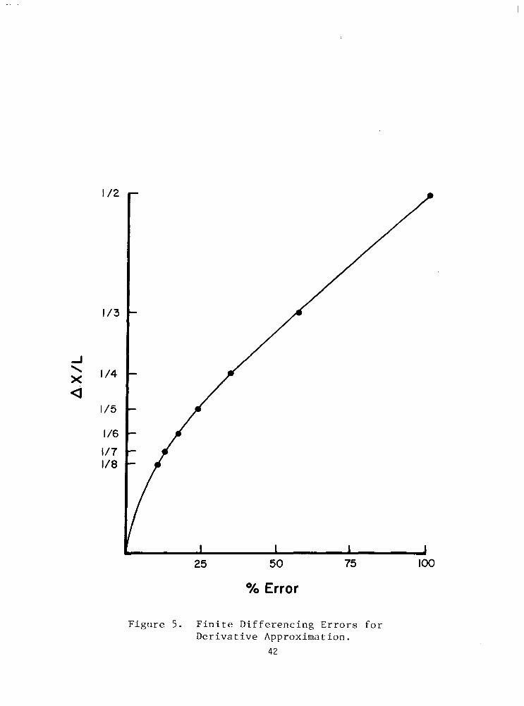
Ax values of c and the resulting error is shown in figure 5. It is Ax obvious that any value of i;- greater than _l. would portray the wave 4

motion very poorly. Thus, one would not want the finite differencing

interval, Ax, to be any larger than t the wavelength or period of the

motion, L, and should preferably be much smaller. This criteria can

now be used as an aid in assigning proper differencing intervals for

the Diurnal Experiment data.

First consider the vertical derivatives. Horizontal winds and

temperature are reported at every km roughly between 30 and 60 km.

From the scaling arguments of the previous chapter, a mean observable

vertical wavelength was chosen at 15 km. Considering the above

criteria, the largest advisable vertical differencing interval would

be 4 km, but preferably much smaller. However, the possibility also

exists for seeing features of smaller vertical scale in the data, for

example, 8 lan features. This would then suggest a differencing

interval of 2 km or smaller. From the point of view of scaling and

potential induced errors, it would not be unreasonable to choose a

vertical differencing interval of 1 km.

For the time derivative, the data covers a 24 hour period and is

reported approximately every 3 hours. From the scaling arguments, a

time period of 12 hours was chosen as the mean observable feature.

Reference to the,above criteria, however, immediately suggests that

the time period suggested by scaling is perhaps too ambitious for this

particular data set with only 4 observations comprising any given 12

hour period. At best, this data set must be considered minimal for

41

l/3

l/6

l/7 l/8

25 50 75 loo

% Error

Figure 5. Finite Differencing Errors for Derivative Approximation.

42

accurately observing a semidiurnal period wave. On the other hand,

theory suggests that the semidiurnal tidal component should be a

significant part of the motion in the region of the atmosphere being

studied. One has little choice under these circumstances but to

choose 3 hours as the time differencing interval if one has any

intentions of depicting the 12 hour time period waves.

At this point, one must take into account another aspect of the

calculation problem. Measurement techniques for atmospheric variables

such as wind and temperature are subject to many random errors, espe-

cially for the middle atmosphere. These errors show up in the data

as high frequency noise which can contaminate any subsequent results.

Since 1 km in the vertical and 3 hours in time represent the highest

frequencies available from the present data set, one might suggest

that the magnitudes of derivatives calculated over such intervals

could be contaminated with noise. This, indeed, is a possibility but

the potential problem can be alleviated somewhat by either smoothing

the data before it is used in the calculations or by increasing the

size of the finite differencing interval. Both of these operations

could have serious drawbacks, though, when the number of data points

is small. While smoothing or differencing over a few lams in the

vertical would affect only a small proportion of the observable wave-

lengths for the present data set, any smoothing or differencing over

more than a 3 hour interval in time could seriously affect all the

possibly observable wave periods. Thus, for this particular data set,

any such operation in the time domain must be used very sparingly or

not at all.

43

Considering the above discussion, the following two calculation

schemes have been adopted for use with the Diurnal Experiment data.

The first, referred to as scheme A, attempts to get as much information

concerning the smaller time and space scale features as possible. For

this purpose, vertical derivatives have been approximated over a 1 km

interval (2Az = 1 km; see equation (3.1))and time derivatives have

been approximated over a 3 hour interval (2At = 3 hours). All calcu-

lated quantities are assigned to the center point of the given time or

space interval (see figure 6). Also, in an attempt to filter out

some,of the potential high frequency noise, the input data has been

smoothed over 3 points (2 km) in the vertical using a l-2-1 filter.

The second scheme, referred to as scheme B, approximates the

vertical derivatives over a 2 km interval (2Az = 2 km) and the time

derivatives over a 6 hour interval (2At = 6 hours), the only exception

being the end intervals in both the time and space domain where the

1 km and 3 hour intervals are again used. This is necessary, espe-

cially in the time domain, to ensure sufficient results to analyze.

Again, all calculated quantities are assigned to the center of the

space or time interval (see figure 6). The input data is smoothed

in the vertical as above. Besides filtering out more of the potential

noise, scheme B should filter out some of the higher frequency infor-

mation leaving larger time period motions and larger vertical wave-

lengths more prevalent in the results. By comparing the results from

the two schemes,one should obtain information concerning the sensitiv-

ity of the results to changes in finite differencing intervals as well

as information as to which scales of motion are dominant. As

44

0 0 0 0

X X X

0 0 0 0 E m .- X X X SCHEME A

I” -- 0 0 0 l

3 X X X

-- l 0 l l

6 ’ I 3 Hrs. I

Time

I 3 Hrs. ’

Time

Figure 6. Finite Difference Schemes: Dots Represent Data Points, X Represents Assigned Position of Calculated Quantities, X Represents Assigned Position of Calculated Quantities on the Boundaries.

45

discussed in the next section, this will aid in the process of judging

how good the results actually are.

One additional consideration in the application of these calcu-

lation schemes is the handling of missing data. While observations

of wind and temperature were to be taken about every three hours for

an entire diurnal period at each station, the usual problems such

as bad weather or payload failure deemed this goal unrealizable. The

result was that all stations except for Kourou missed at least one

temperature measurement and a few stations missed both temperatures

and wind measurements for the given observation period. In such

cases, the following rules were adhered to. If only a temperature

observation was found missing, values were linearly interpolated from

the neighboring values in time and calculations proceeded as normal.

If both temperatures and winds were missing for the same observation

period, no interpolated values were assigned but the finite difference

interval in time was increased over the affected time periods. This,

in essence, served as a linear interpolation of the time derivatives.

It was felt that these rules would subject the data set to the least

amount of manipulation while still ensuring a reasonable amount of

continuity in the calculations over the affected time periods. A

list of those time periods affected at each station is given in Table 2.

46

TABLE 2. Missing Data Log

Station ~------

Kourou

Fort Sherman

Ascension

Antigua

Natal

Time Period of Interpolated Time

------+

Periods of Missing Temperatures (GMT)_ Temperatures and Wind (GMT)

2100 0000

0400 -

3.2 VERIFICATION SCHEME

Up to this point, much of the emphasis has been placed upon de-

riving a single station technique for calculating vertical velocities.

While this has been achieved, an equally important aspect of the

problem has been neglected, namely, how does one determine whether

the results are valid? One obvious approach would be to compare the

derived vertical velocities to actually observed values, but this

possibility has already been discounted. Another approach would be to

compare the results to those derived via an alternate vertical velocity

equation, but the characteristics of the present data set preclude

this possibility.

One method which can be used for this study is to compare the

derived vertical velocities to results suggested by theory. Along

this line, two questions must be considered:

47

1) Are the results physically reasonable?

2) Do the results match current models?

The first question can be approached in several ways. For example,

it is generally accepted that real atmospheric features should show

some continuity in time and space. If the derived vertical motion

fields do not show this continuity, the validity of the results might

be questioned. Another approach deals with the assumption that the

results resemble some form of internal gravity wave motion. It is

generally accepted that the magnitude of upward propagating wave type

motion should increase with height as p -l/2 where p is the density.

Thus, one would expect the derived vertical motions to verify this

relation.

To answer the second question, one must have a model to which the

results can be compared. Such a model is available in the theory of

atmospheric tides but the limitations of the present data set subject

this type of analysis to much uncertainty. In order to directly

compare the derived vertical motions to the tidal predictions, the

vertical motion fields must be decomposed into their diurnal and semi-

diurnal components, a procedure which can create much error with only

eight data points covering the entire diurnal period. Still, this

analysis will enable one to draw many general conclusions concerning

the derived vs. predicted vertical motions.

The scaling arguments of the previous chapter afford an indirect

means of comparing the derived vertical velocities to tidal predic-

tions. Since the time and length scales chosen for the analysis were

those suggested by tidal theory, one could compare the calculated mag-

nitudes of the various terms in equation (2.18) to those suggested by

48

the scaling arguments. A necessary condition for the observed

motions to be tidal would then be that the various terms agree at

least in order of magnitude. If they do not, then one must question

either whether tidal type motions are being observed or whether the

vertical velocity equation is in the proper form for this particular

study. This internal consistency check, however, can only serve as

a necessary and not a sufficient condition for the observed motions to

be classified as tidal, etc., since the time and length scales used

could represent other types of motion as well.

The next step in the verification process is to consider the

numerical aspects of the calculations. Two more questions arise:

3) Are the results numerically stable?

4) Are the results significant with respect to the errors of

measurement?

In reference to the third question, one would expect good

results to be relatively insensitive to changes in the calculation

scheme. For example, change in the data smoothing procedure or finite

differencing interval should not greatly affect the overall results.

For the present study, this criteria will be checked by comparing the

results obtained via the scheme A and scheme B calculationprocedures

discussed earlier in this chapter.

In many ways, the fourth question serves as the final judge of

the validity of any results, for if the magnitudes of the results

are smaller than the magnitudes of the numerical errors, then the

results must be invalidated despite any previous conclusions. The

next step in the methodology is thus to derive a scheme by which these

numerical errors can be accounted for.

49

Numerical errors can come from three distinct sources:

1) Errors inherent in the data set, usually referred to as noise.

2) Errors introduced by neglecting terms in the generalized

equation.

3) Errors inherent in the finite differencing scheme used.

The first type of error can be accounted for by considering the

characteristics of the measuring devices and procedures. In this case,

the measured winds and temperatures are considered repeatable to with-

in 2 3 m/set and + 1°K respectively. Errors derived from neglecting

terms in an equation are accountable by referring to scaling argu-

ments. Both of these forms can be included in a single expression

which will be derived below. Errors inherent in using a given finite

difference scheme must be considered subjectively, however, as one

is never quite sure what scales of motion are being observed.

The expression for estimating the error can be derived by taking

the vertical velocity, w, to be a function of four independent vari-

ables; the local time derivative of temperature (DTDT), the horizontal

derivative of temperature (ADVT), diabatic heating (DIAB), and stability

(STAB):

w = DTDT + ADVT + DIAB STAB . (3.4)

By forming the total differential of w, 6w, the error expression

becomes:

6w = & [~(DTDT + G(ADVT) + ~(DIAB)]

_ (DTDT + mv~ + DIAB) &STAB

(STAB)~ (3.5)

50

One is usually interested in the maximum error obtainable. Thus, each

term in the above expression should contribute positively to the whole.

To ensure that this happens, the expression is usually squared. Then,

assuming that the errors are random, cross terms drop out, leaving:

fjw =

I

(~DTDT)~ + (~ADVT)~ + (~DIAB)~ ___-- (STAB)2

+ (~STAB)~ (DTDT + mvT + DIAB): 1 112

(sTAB)~ J - (3.6)

Equation (3.6) is the expression for the absolute error. Relative

error may be calculated by dividing the above expression by w. A

more representative value to use, however, is the root mean square of

the error:

6W ST =

N c 6w.2

i=l ’ N

l/2

, (3.7)

where N represents the number of points being summed over.

Using the + 1°k and 2 3 m/set accuracy estimates previously

stated, one can now assign specific values to each error term in

equation (3.6). The details of this procedure are reviewed in

Appendix C, the results of which are suggested below.

G(DTDT) = 1%/3 hours

A(ADVT) = 0.3 (ADVT)

6(DIAB) = 0.2 (DUB)

15 (STAB) = 0.5°K/km

(3.8)

51

Substitution of these values in equation (3.6)-yields the final form

of the error equation used for this study:

6w = lo-8"

[

k/set + 0.09 (mvT12 + 0.04 (IIIAB)~

STAB2

0.25(w) 2

+ STAB4

1 112 . (3.9)

At each altitude, the above calculated values are summed over time as

in equation (3.7). This yields a vertical profile of error estimates

to which the actual vertical velocities can be compared.

Since direct measurements of vertical velocities are unavailable

for comparison with the derived values, the verification procedure

developed over the last several pages cannot be expected to give the

final judgment over the results. It is felt, however, that if the

above four questions are considered carefully and all the evidence is

collectively weighed, some fairly definite conclusions can be drawn

concerning the vertical motion fields for the Diurnal Experiment.

52

4.0 RESULTS AND DISCUSSION

Over the past two chapters, a scheme has been developed to both

calculate and analyze vertical motions in the equatorial middle at-

mosphere. This scheme has been used along with the Diurnal Experiment

data set to calculate vertical motions at Kourou (French Guiana), Ft.

Sherman (PCZ), Natal (Brazil), Antigua (BWI), and Ascension Island.

The purpose of this chapter is to present and discuss these results.

This will be accomplished in three steps. First, time series cross

sections will be presented and discussed with respect to the numerical

stability and error criteria of the previous chapter as well as to the

identification of prominent features continuous in space and/or time.

The next step will be to check the internal consistency between the

calculated magnitudes of terms and those suggested by the scaling

arguments of Chapter 2. Finally, the results will be compared to the

predictions of atmospheric wave theory, specific reference being made

to the predictions of atmospheric tides.

4.1 TIME SERIES CROSS SECTIONAL ANALYSIS

Time series cross sectional analysis is perhaps the most straight-

forward means of depicting continuous features in a given data set.

If the data is made up of various wave forms, however, one must be

sure that it is properly presented on the cross sections to depict

these features. The following considerations are especially important.

First, wave motion almost always appears as perturbations on a mean

flow. Thus, in cases where the mean varies over the study range,

perturbation values of the derived field quantity should be used.

53

Secondly, if waves with periods larger than can be depicted by the

data set form a significant part of the motion, they can appear as

linear trends in the data. If one is interested only in those par-

ticular waves which can be completely depicted by the data, then these

linear trends must also be removed.

The diurnal means of the derived vertical motions at each altitude

are presented for scheme A in Table 3. One will note that the magni-

tudes vary irregularly over the altitude range but do show a tendency

to increase with height. The magnitudes as calculated for scheme B

are slightly smaller but the tendencies are roughly.the same. Since

wave forms are expected in the data it therefore does appear advisable

to use perturbation values in the cross sections. These will be

defined relative to the diurnal mean as follows:

W’ =w-w (4.1)

where w' represents the perturbation quantity and w represents the

diurnal mean.

At this point in the analysis, interest will not be limited only

to wave features which can be completely depicted by the data set, for

evidence of wave periods greater than 24 hours would be as significant

a result as the depiction of the tidal fields. Therefore, linear

trends are not removed from the cross sectional data. This subject

will again be brought up later in the chapter when an attempt is made

to decompose the results into the various tidal components.

The time series cross sections of the perturbation vertical

motions for Kourou, Ascension Island, Ft. Sherman, Antigua and Natal

54

TABLE 3. Diurnal Means of Vertical Velocity, Scheme A (cm/set).

Height (km) Kourou pt. Sherman lscension Antigua Natal 63 62 61 60 59 58 57 56 55 54 53 52 51 50 49 48 47 46 45 44 43 42 41 40 39 38 37 36 35 34 33 32 31 30 29 28 27 26 25

2.5 2.4 1.1 0.3 0.1

-1.1 -1.4 -1.0 -0.3 -0.1 -0.1

0.4 0.4 0.6 0.4 0.4 0.4 0.4 0.1 0.5 0.5 0.1

-0.1 -0.1

0.0 -0.5 -0.0

0.0 -0.1

0.3 0.1 0.2 0.3

-0.2 -0.9 -1.4 -1.5 -0.9 -0.3

0.4 0.4 0.4 0.4 0.3 0.4 0.3

-0.1 -0.8 -0.8 -0.1 -0.2 -0.1

0.2 0.2

-0.7 -0.9

0.4 1.7 0.8 0.1 0.1 0.2

0.3 1.0 2.4 2.2 0.2

-0.3 -0.9 -0.2

0.3 0.5 1.6 1.6 1.0 0.3

-1.0 -1.2 -1.0 -0.5

0.4 -0.1 -0.1

0.3 0.8 1.3 1.3 0.7 0.1 0.1 0.2 0.6 0.5

-0.0 -0.2 -0.0

1.3 2.8 3.0 1.8 1.7 1.4 0.4

-0.4 -1.0 -0.3

0.5 0.8 0.1

-0.5 -0.1 -0.3 -0.2 -0.2 -0.1

0.1 -0.1 -0.1

0.0 -0.2

0.2 0.4 0.2

-0.5 -0.3 -0.1 -0.0 -0.3 -0.2

1.0 -1.5 -0.6 -0.3

0.1 1.0 0.8 0.4 0.1 0.2 0.6 0.9 0.9 0.5 0.1

-0.1 0.4 0.3 0.6 0.8 0.7 0.7 0.1 0.1 0.7 0.3 0.5 0.7

-0.0 -0.1 -0.1

0.0

55

are presented in figures 7 through 11. In each of these figures, the

A part corresponds to the results for scheme A and the B part corre-

sponds to the results for scheme A and the B part corresponds to the

results for scheme B. The cross sections have been analyzed to depict

the positive (shaded) and negative (unshaded) areas of vertical motion.

An inspection of the cross sections suggests that some sort of

gravity wave type motion is being depicted. In general, the waves

seem to have diurnal, semidiurnal, and even shorter time periods with

amplitudes increasing from 1 or 2 cm/set at 30 km to as large as 15

cm/set near 60 km. In addition, it appears as if the cross sections

can be classified into two distinct groups. In group I, including

Kourou, Ft. Sherman, and Ascension, the dominant wave features are

characterized by relatively short vertical wavelengths (15-20 km)

and an evident downward phase progression (20-50 km/day). In group II,

including Natal and Antigua, the dominant wave features are charac-

terized by relatively long vertical wavelengths (> 20 km), a mainly

diurnal period, and little or no evident phase progression. These

group designations prove to be an unexpected but interesting feature

in the results and will be discussed further below.

The fact that features as suggested above can clearly be seen in

the cross sections gives some initial credence to the results. These

features must be compared to atmospheric wave theory in a more quan-

titative fashion, though, before one classifies the results as

physically acceptable. This will be done later in the chapter, but

first it is advisable to check the numerical stability and error

criteria suggested in section 3.2.

56

-

60 -

55 -

50 -

s45 Y

-

5 - (3 Y 5

40 -

35 -

30 -

25 -

-0.4 ' -5.5 : -4.2 ,'

2.4 ~-7.2 -6.3 !

-12.5 1 -5.8,il

-1.5 - -1.8 -0.j -2;3

I- 1 1.9

A 1.7 1.3 1.4 2.0 2.0 1.6

- 1.4 1.4

i 1.3 1.2 1.2 1.2 1.1 1.1 1.1 1.2 1.2 1.2 1.0 0.7 0.7 0.7 0.8 0.8 0.8 0.8 0.8 0.8 0.9 1.0 0.9

1500 1800 2100 0000 0300 0600 0900 1200 1500 Errors TIME (GMT)

FIGURE 7A. Vertical velocities and error estimates for Kourou, scheme A (cm/set).

60 -

55 -

50 -

s445 - Y -

!G '3 Id I

40 -

35 -

30 -

-1.4 -7.3 -2.5

-2.4 -1.77 -2.7 -0.7 -3.8 -1.1 F -4.3 -2.4 -3.1 I- --3-7 I -2.6 \ -5.i\, -1.

-0.6 -1.9 -0.5 -2.0 -0.6 0.0 -0.3

25 I I I I I I I I I

1500 1800 2100 0000 0300 0600 0900 1200 1500 TIME (GMT)

1.8 1.7 1.4 1.3 1.5 1.9 1.7 1.4 1.3 1.3 1.2 1.2 1.2 1.1 1.0 1.1 1.1 1.2 1.2 1.1 0.8 0.7 0.1 0.7 0.7 0.1 0.8 0.8 0.8 0.9 0.9 0.9 a.9

Errors

FIGURE 7B. Vertical velocities and error estimates for Kourou, scheme B (cm/set).

l- I I I I I I I I I

55

50

35

30

25 -1.0

1 I I I

1.6 1.8 1.8 1.7 1.5 1.5 1.5 1.4 1.3 1.5 1.4 1.3 1.1 1.1 1.2 1.0 0.9 0.9 0.9 0.9 0.9 0.8 0.8 0.9 1.0 0.9 0.9 0.9 0.9 1.0 0.9 0.9 0.9

1500 1800 2100 0000 0300 0600 0900 1200 1500 Errors TIME (GMT)

FIGURE 8A. Vertical velocities and error estimates for Ascension Island, scheme A (cm/set>.

60 60 _

5 x45 -

i-

2 al 0 iii

I

40 40 -

25 25 -

b-o.3 J -2-i

0.0 ,'-6.2 '\ f-8.6 , ' -8.5 '.-7 2 /' .1/

prd -3.2 -L-l ..-

f63-i &iiJ

-3.0

-0.3

\ -2.7

^- \ -0.1

3.7 ; 2.3 1.4 4.4 n-A 2.8

.3.u ---

.' 0.9 ' 2.4 Ll.8 -2.8 . 3.. a 1.2 1.6 0.6

-1.3 -0.7 118 a.2

\ I

-0.1 -2.3 -0.4 -1.3 -3.2 -1.2 0.1 -1.8

, /:5-y?\ . -2.2 0.0 -0.9 -..- _ ; -1.0

-0.5 -0.9

.I.6 ‘0.8 1.3. -1.9 n.n 1.0 -0.9

I I I I I

1.3, a 2.7 -2.3 -0.8 2 -1.3 -0.8

-2.6 -1.8 -1.1 -0.7 -1.7

-0.4 h -2.7 -0.9 -0.8 -0.9

1500 1800 2100 0000 0300 0600 0900 1200 1500 TIME (GMT)

1.3 1.3 1.5 1.6 1.5 1.4 1.5 1.3 1.2 1.3 1.3 1.2 1.1 1.1 1.1 1.0 0.9 0.8 0.8 0.8 0.8 0.8 0.8 0.8 0.9 0.9 0.9 0.9 0.6 0.9 0.9 0.9 0.9 0.9

Errors

FIGURE 8B. Vertical velocities and error estimates for Ascension Island, scheme B (cm/set).

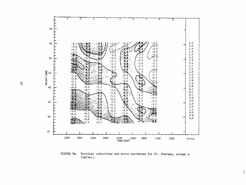
60

55

50

5 45 Y l- 3 $

40

35

30

25

1500 1800 2100 0000 0300 0600 0900 1200 1500 TIME (GMT)

1.3 1.4 1.5 1.4 1.3 1.2 1.0 1.1 1.1 1.1 1.0 1.0 1.0 1.0 1.0 0.8 0.7 0.7 0.7 0.8 0.9 1.0 0.9 1.2 0.9 0.8 0.9

Errors

FIGURE 9A. Vertical velocities and error estimates for Ft. Sherman, scheme A (cm/set).

60 -

55 -

50 -

f y 45 -

$

z I

40 -

35 -

30 -

J3y 1.5 m&S< 2.3 -1.8 -0.9 -2.4 -2.6

&nS 2.9 Q

-1.2 -1.0 -1.6 -3.0 -0.3 ‘is 3.1 -0.7 -1.1 -3.4 -2.4

-3.6 -3.0 -3.0 -4.1

25 I I I I I I I I I

1500 1800 2100 0000 0300 0600 0900 1200 1500 TIME (GMT)

1.3 1.4 1.5 1.4 1.3 1.2 1.1 1.1 1.1 1.1 1.1 1.0 1.0 1.0 0.9 0.9 0.8 0.7 0.7 0.7 0.8 1.0 0.0 1.1 0.9 0.8 0.8 i 0.9

I

FIGURE 9B. Vertical velocities and error estimates for Ft. Sherman, scheme B (cm/see).

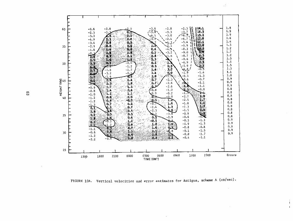
60 -

55 -

50 -

845 - Y - I- _ 3 _

i! - 40 -

35 -

30 -

25 - I I I I I I I I I 150,O 1800 2100 0000 0300 0600 0900 1200 1500

TIME (GMT)

1.8 1.9 1.9 1.6 1.4 1.3 1.2 1.7 1.2 1.3 1.5 1.5 1.3 1.1 1.0 0.9 0.9 0.9 0.8 0.8 0.8 0.8 0.8 0.8 0.8 0.8 0.8 0.9 0.9 0.9 0.9 0.9

Errors

FIGURE 10~. Vertical velocities and error estimates for Antigua, scheme A (cm/set>-

r I I I I I I I I I

60 - ;4AO -5.2- - -4:1\, -3.2, -2.9 \

55 -

-3.1 -3.5

-=q -5.2 -5.3 -5.9 -6.3 -6.0

-2.3 \ -1.9 \ -1.9 ’ -1.6

50 -

,2.4 1.0 b.8

5 x45 -

I- 3 ii I

40 -

0.9 1.3 CPA--o.3 2.i 2.; 0.9 1.1 0.8 0.6 c 0: 0.2 0.6 &

-0. -1.3

35 -

30 -

23:; .‘I 2.5‘ i:j

_. -0.

0.3 0.0 0.9 ---\oI; 0.6 '. 0.3 1

GO.2 -0.73 0.2 '0.3 .O*Q ,.o*!r t:

2:; ---xii / cicri-- ".>

-0.7 ----&J : 1.0 1.4 0.7 1.3 -1.9 -0.A I

25 - , I I I I I I I I I

-1.6 -2.0 -3.5 -4.2 -2.7

-

1.7 1.8 1.9 1.7 1.5 1.4 1.3 1.2 1.2 1.2 1.4 1.4 1.3 1.2 1.0 0.9 0.9 0.9 0.0 0.8 0.8 0.8 0.8 0.7 0.8 0.8 0.8 0.8 0.0 0.9 0.9 0.9 1 . 0

1500 1800 2100 0000 0300 0600 0900 1200 1500 Errors TIME (GMT)

FIGURE 10B. Vertical velocities and error estimates for Antigua, scheme B (cm/set).

60

55

50

40

35

30

25

I I I I I I I I I

U.1 3

.‘I \

-1.0 b . -0.0

- -0.4

~~

-2.3 -0.4 -0.7 -1.7 -0.0 . , \. $:F

1 I I I I I I I I I

1500 1800 2100 0000 0300 0600 0900 1200 1500 TIME (GMT)

2.0 1.8 1.7 1.6 1.5 1.3 11 1.2 1.2 1.2 1.3 1.3 1.2 1.0 0.9 0.8 0.7 0.7 0.8 0.9 0.8 0.8 0.8 0.9 0.9 0.9 0.9 1.0 0.9 0.8 0.8

Errors

FIGURE 11A. Vertical velocities and error estimates for Natal, scheme A (Cm/Sed.

60 -

55 -

50 -

z 45 - t- 5 w I

40 -

35 -

30 -

25 -

-1.7 -1.6 -1.2

-1.2 -1.8 -1.6 -1.9

-0.5 -1.0 -0.9 -1.6

I I I I I I I I I 1500 1800 2100 0000 0300 0600 0900 1200 1500

TM (GMT)

1.7 1.5 1.6 1.5 1.4 1.3 1.2 1.2 1.2 1.2 1.2 1.2 1.2 1.0 0.9 0.8 0.7 0.7 0.7 0.8 0.8 0.8 0.8 0.9 0.9 0.9 0.9 1.0 0.9 0.8 0.8 0.8

Errors

FIGURE 11B. Vertical velocities and error estimates for Natal, scheme B (cm/set).

As indicated in the previous chapter, none of the results can be

accepted unless they are first shown to be significant with respect to

the numerical error estimates. To check this, vertical profiles of the

root mean square as calculated from equations (3.9) and (3.7) have

been included to the right of each cross section in figures 7 through

11. One will note that the relative error is quite small in all but

perhaps the lower third of the altitude range (< 40 km). Even in this

lower range, though, the error estimates are small compared to the

maxima and minima of the vertical velocity patterns. Thus, upon con-

sideration of this one criteria, it is felt that the general magnitudes

and patterns of vertical velocities depicted in the cross sections can

be accepted with little hesitation.

It has also been suggested in the previous chapter that for the

results to be acceptable, they should be relatively insensitive to

changes in the calculation scheme. This criteria will now be checked

by comparing the results obtained using scheme A and scheme B. In-

spection of the cross sections shows that the magnitudes of the verti-

cal velocities calculated using scheme B are slightly smaller than

those of scheme A. Also, some of the smaller time and space scale

features appear slightly smoothed out in the scheme B cross sections.

This smoothing effect, however, is exactly what one would expect if

the observed motions were composed of semidiurnal or even smaller

period waves along with the diurnal waves, or if the data contained

significant amounts of high frequency noise. The increased finite

differencing interval used in scheme B decreases the magnitudes of

the derivatives for the smaller period motions. But since the

67

differences between the two schemes is generally small, it is felt

that the results can be accepted relative to the sensitivity criteria.

Another question which must be considered when comparing the

cross sections among the different stations is how the several cases of

missing data affect the calculations. While most of the calculations

have been done with a three hour interval between observation times,

Ascension, Antigua, and Natal each have one observation period missing.

For this particular time period, the calculations proceed as usual

around the missing data by adding the additional three hours onto the

time differencing interval. To see how this affects the results, a

test calculation has been made for Kourou with the OOOOZ data left out.

The results for scheme A and scheme Bare presented in figures 12A and

12B respectively. Comparing these with figures 7A and 7B, one notes

that the actual magnitudes of the vertical velocities have changed over

the affected time periods but the overall difference is a general

smoothing out of the smaller time scale features. Since smaller time

scale features cannot be depicted well by the present data set in any

case, this type of induced error will be considered acceptable for this

analysis.

4.2 INTERNAL CONSISTENCY

The next step in the analysis is to check the internal consistency

between the calculated magnitudes of the terms comprising equation

(2.18) and the estimated magnitudes suggested in equation (2.16A).

Since the scaling arguments used characteristic values from about

the 45 km level, the comparison should likewise be made with calculated

68

60 -

55 E

1

50 -

L 7

z45 L

I- - z ii I

40 -

35 -

30 -

25 -

1500 1800 2100 0000 0300 0600 TIME (GMT)

1.8 1.6 1.3 1.4 2.0 2.0 1.6 1.4 1.4 1.3 1.2 1.2 1.2 1.1 1.0 1.1 1.2 1.2 1.2 1.1 0.8 0.7 0.7 0.8 0.8 0.8 0.8 0.8 0.8 0.9 1.0 0.9

0900 1200 1500 Errors

FIGURE 12A. Vertical velocities and error estimates for Kourou, 00002 data left out, scheme A (cm/set).

60 -

55 -

50 -

$45 -

i= 5 _ P -

40 -

35 -

30 -

-1.7 0.7 1.4 0.8 1*9 LO 1.6 0.9

25 I I I I I I I I I

1500 1800 2100 0000 0300 0600 0900 1200 1500 TIME (GMT)

1.8 1.7 1.4 1.3 1.5 1.9 1.7 1.4 1.3 1.3 1.2 1.2 1.2 1.1 1.0 1.1 1.1 1.2 1.2 1.1 0.8 0.7 0.7 0.7 0.7 0.7 0.8 0.8 0.8 0.9 0.9 0.3 0.9

Errors

L.

FIGURE 12B. Vertical velocities and error estimates for Kourou, OOOOA data left out, scheme B (cm/set).

magnitudes from this altitude range; However. it would also be useful

to see how the calculated magnitudes vary with height. Considering

this, the following approach has been taken.

The range of height at each station has been divided into three

equal (s 10 km) sections. Since the calculations generally run

between 30 and 60 km, these divisions can be thought of as representing

the mid-stratosphere (30-40 km), upper stratosphere (40-50 km), and

lower mesosphere (50-60 km). To obtain a characteristic magnitude of the

various terms for each of the three divisions, the absolute value of the

terms were averaged over time and height for each 10 km layer. The re-

sults for scheme A and scheme B are presented in Tables 4 through 6. The

terms have been designated as in equation (3.4) with the exception that

the horizontal advection of temperature has been split into its

geostrophic and ageostrophic parts.

(ADVT)G E 2 (YH x 2) l ;t

(4.2)

For consistency and ease of analysis, the terms in the numerator

have been divided by the stability term. This puts all the terms

into units of cm/set as in equation (2.16A). In this procedure, the

characteristic magnitudes from the upper stratosphere division will be

the ones used for comparison with the scaling magnitudes.

First, it will be useful to check the scaling consistency crite-

ria. Referring to Table 5, it appears as if the heirarchy of contri-

buting terms is as suggested in the scaling arguments with DTDT being

71

TABLE 4A. Mean Magnitudes for Middle Stratosphere, Scheme A (cm/set>.

Kourou

Ft. Sherman

Ascension

Natal

Antigua

Average

DTDT

1.3

0.7

1.6

0.8

0.8

1.0

DIAB

0.4

0.5

0.5

0.5

0.4

0.5

(ADvT)~

0.3

0.7

0.7

0.4

0.5

0.5

(ADVT)

0.1

0.2

0.2

0.1

0.3

0.2

TABLE 4B. Mean Magnitudes for Middle Stratosphere, Scheme B (cm/set).

Kourou

Ft. Sherman

Ascension

Natal

Antigua

Average

DTDT

1.0

0.6

1.2

0.7

0.7

0.8

DIAB

0.5

0.5

0.5

0.5

0.5

0.5

(ADVT)*

0.2

0.6

0.4

0.3

0.3

0.4

(ADVT)

0.1

0.1

0.2

0.1

0.3

0.2

w

1.5

1.2

1.5

0.8

1.1

1.2

W --

0.9

0.7

1.0

0.6

0.8

0.8

72

TABLE 5A. Mean Magnitudes for Upper Stratosphere, Scheme A (cm/set).

Kourou

Ft. Sherman

Ascension

Natal

Antigua

Average

Scaling

DTDT ---

2.8

1.9

2.2

1.3

1.2

1.9

10.0

DIAB

0.8

0.7

0.7

0.7

0.8

0.7

1.0

(ADVT) ag (ADVT)g

0.4 0.1

0.3 0.1

0.7 0.2

0.4 0.1

0.4 0.2

0.4

1.0

0.1

0.1

TABLE 5B. Mean Magnitudes for Upper Stratosphere, Scheme B (cm/set).

DTDT DIAB

Kourou 1.6

Ft. Sherman 1.4

Ascension 1.8

Natal 1.0

Antigua 0.9

Average 1.3

Scaling 10.0

0.8

0.7

0.7

0.7

0.8

0.7

1.0

(ADVT)~

0.2

0.2

0.5

0.3

0.2

W

3.6

1.8

2.4

1.8

1.6

2.2

10.0

73

TABLE 6A. Mean Magnitudes for Lower Mesosphere, Scheme A (cm/set).

Kourou 5.0

Ft. Sherman 2.6

Ascension 3.7

Natal 2.9

Antigua 2.7

Average 3.4

DTDT DIAB

1.1

0.9

1.0

1.0

1.1

1.0

(BVT) ag (mVT) g

0.8 0.2

0.2 0.1

1.6 0.4

1.0 1.0

1.0 1.1

0.9 .O. 6

TABLE 6B. Mean Magnitudes for Lower Mesosphere, Scheme B (cm/set).

Kourou

Ft. Sherman

Ascension

Natal

Antigua

Average

DTDT -____

3.7

2.1

2.4

2.0

2.4

2.5

DIAB ..~-

1.0

0.9

1.0

1.0

1.1

1.0

:ADVT) ___ _ 32

0.7

0.1

1.0

0.6

0.7

0.4

(ADVT ‘g ----

0.2

0.1

0.4

0.2

0.5 ~-.

0.3 --._-__ _-

W -~- ----

5.7

3.6

5.1

4.2

3.9

4.5

W

4.5

2.8

2.9

2.5

3.9 ----

3.3 -.----

74

I

the major contributor, but the calculated mean magnitudes appear to

be smaller than those suggested by scaling. This can be explained

somewhat by accounting for negative contributions among the various

terms in the actual calculations, but not entirely. Another possibil-

ity is that the scaling values are wrong and upon reviewing the

scaling arguments, one particular value becomes chief suspect, namely,

the time scale. It was assumed in section 2.3 that a mean observable

time scale would be 12 hours. If a 24 hour period had been used

instead, the scaled magnitudes for DTDT, (ADVT) 4s'

and subsequently,

w, all would be decreased by a factor of 2. This would now bring the

scaled and calculated magnitudes all within the same range. This

would suggest that a diurnal period wave is being depicted in the

data as well as semidiurnal or shorter period waves. Indeed, this

is what the cross sections seem to suggest. Thus, by using the larger

time scale, the calculations and scaling arguments become internally

consistent with each other.

For the lower mesosphere region (Table 6), one finds the same

hierarchy of terms with DTDT clearly dominating the calculations. The

magnitudes of all the terms are larger than for the upper stratosphere,

but this is merely consistent with the theory of atmospheric waves

which suggests that amplitudes should increase with height as p -l/2 ,

p being the. density. In much the same way, the magnitudes of the

terms for the middle stratosphere (Table 4) are found to be smaller

than those for the upper stratosphere. Here again, the calculations

are dominated by the DTDT term, but not by as great a margin as in the

previous cases.

75

The apparent dominance of the calculations by the DTDT term

suggests a shortcut in the vertical velocity calculations by neglecting

all the terms in the numerator of equation (2.18) except for DTDT.

To see how such a scheme would work, a test calculation was made for

Kourou, the results of which are presented in figure 13A and 13B.

A comparison with figures 7A and 7B demonstrates that while the

magnitudes of the vertical velocities have changed slightly, the major

features have remained well intact. This technique may thus prove to

be quite useful in short time scale high altitude studies where wind

measurements are inaccurate or missing entirely.

4.3 COMPARISON WITH ATMOSPHERIC WAVE THEORY

So far, the results have been demonstrated to be acceptable with

respect to the numerical stability, error estimates, and internal

consistency criteria. This, along with the continuous periodic

features evident in the cross sections suggests that the derived

vertical motions are real and are of the tidal or other internal

gravity wave type. The goal of this section is to discuss these

results in the context of atmospheric wave theory.

An often stated postulate of atmospheric wave theory is that

the amplitude of an upward propagating gravity wave should increase

with height as p -l/2 , p being the ambient density. This condition is

necessary to ensure the conservation of kinetic energy. The first

step in this analysis will be to test this relationship for the

current results. For this purpose, a plot has been made of the maximum

amplitude of the vertical velocity for the diurnal period versus

height for each of the cross sections in figures 7A through 11A. The

76

60 -

55 -

50 -

35 -

30 -

25 -

1

I I I I I I I I I I

1500 1800 2100 0000 0300 0600 0900 1200 1500

TIME (GMT)

FIGURE 13A. Vertical velocities for Kourou as calculated with only local temperature change term, scheme A (cm/set>.

L I I I I 1 I I I I

60 -

55 -

50 -

545 - Y I- 6 Gi I

40 -

35 -

30 -

3 -~ x Ii3 \ -4.1 -1.8 -3.4 -1.5

7,, y*- -0.5 -1.4 -1.8 -1.0 -0.7

25 I I 1 I I I I I I

1500 1800 2100 0000 0300 0600 0900 1200 1500 TIME (GMT)

FIGURE 13B. Vertical velocities for Kourou as calculated with only local temperature change term, scheme B (cm/set).

results for the Group I and Group II stations are shown in figures 14

and 15 respectively. Only the calculations from scheme A have been

used to ensure that the maximum amount of information concerning the

shorter period'waves is included in the analysis. On each of the above

figures a scaled plot of p -l/2 has been included for easy reference

(see Appendix D for details).

First, for figure 14, one will note that the amplitude variation

with height of the derived vertical motions is similar for all three

stations. The variation follows the p -l/2 curve, but does so in a

sinusoidal fashion. In figure 15, however, both Natal and Antigua

display little amplitude variation below 45 km followed by a sharp

increase in amplitude above this altitude. The net tendency, though,

is to follow the p -l/2 curve quite closely.

It thus appears as if the p -l/2 condition is confirmed, at least

in general, for all five stations in the study. But as with the cross

sections, distinct differences appear between the Group I and Group II

stations. These distinctions could be indicating that other types of

motion are interacting significantly with what appear to be internal

gravity waves or tidal motions. Before this conjecture is discussed

further, it would prove useful to see to what extent the current results

can be explained via tidal theory.

Unfortunately, any attempt to compare real data to tidal theory

is at best a difficult task. One reason for this is the relatively

early stage of the theoretical calculations. In order to obtain

solutions to the tidal equations, many approximations must be made.

Some of the more important ones are listed below:

79

60

30 /- \

- - KOUROU

---- FT. SHERMAN

-------- ASCENSION

I I I I I I I I I I I I I I I I I I 1

5 I

IO 15 20

Vertical Velocity (Cm /Set)

Figure 14. Maximum Magnitude of Vertical Velocity at Kourou, Ft. Sherman, and Ascension.

. . . -,

60

55

50

45

40

35

30

/----- -L-_-m----

I -CL--

- - - NATAL -------ANTIGUA

5 IO

Vertical Velocity Km/Set) 15 20

Figure 15. Maximum Magnitude of Vertical Velocity at Natal and Antigua.

1)

2)

3)

4)

5)

The last

The earth's surface topography is ignored.

Dissipative processes are ignored.

Any longitudinal dependence on the distribution of absorbing

gases is ignored.

Tidal motions are considered to be linear perturbations on a

basic state.

Horizontal temperature gradients are considered to be zero,

implying that the mean flow is zero.

approximation has been relaxed recently for calculations of

the semidiurnal tidal component by Lindzen and kong (1974), but over-

all, the results from tidal theory apply to a highly idealized atmo-

spheric state. For a fairly complete review of the theory, one should

refer to the book, "Atmospheric Tides" by Chapman and Lindzen (1970).

Despite these Limitations, many of the general features of the

theory are found to match observations quite well. (See, for example,

Groves (1975), Schmidlin (1976), Kao and Lordi (1977)). Good agreement

is found with the amplitudes of the various components but a few

differences still exist between the predicted and observed phases of

some of the components.

To some extent, these differences can also be blamed on the

deficient amounts and quality of atmospheric data sets available for

studying tidal motions. Results from tidal theory are presented in

terms of the various diurnal, semidiurnal, terdiurnal, and even

smaller time period modes. Thus, in order to compare observations to

the theory, the data must be decomposed into its diurnal, semidiurnal,

etc., components. Through techniques of Fourier analysis, this can

82

be done with a good degree of acctiracy for sufficiently large data

sets. It is generally accepted that a sufficiently large data set

should have at least 8 data points representing the particular mode

being studied and should also include several complete periods of

that particular mode. Upper atmospheric data sets which satisfy this

criterion are virtually non-existent. Perhaps the best data set for

studying upper atmospheric tides to date is the Diurnal Experiment,

but even here, eight points make up the diurnal period, 4 points make

up a semidiurnal period, and only one diurnal period makes up the

entire sequence. One would therefore not normally consider even the

present data set suitable for tidal analysis. However, since the

Fourier analysis procedure is the best means at our disposal for

comparing the derived vertical motions to tidal theory, this is the

approach which will be taken. But considering the limitations of this

procedure, the results must be analyzed in the context that tidal

theory should be able to explain many but not necessarily all the

features in the derived vertical motion field.

An additional requirement for use of the standard Fourier analysis

routines is the necessity of having evenly spaced data points. For the

Diurnal Experiment data, this condition is met only at Kourou and Ft.

Sherman as the other three stations each have one calculation period

missing. One could conceivably interpolate the vertical velocities

for these time periods but it is felt that this would unduly add more

possible errors on to an already heavily strained analysis. Thus,

the procedure has been carried out only for Kourou and Ft. Sherman.

Also, in order to get an even 8 points for the analysis, scheme B data

83

had to be used for Ft. Sherman while scheme A data could be used

for Kourou.

The particular scheme used is described in Appendix E and includes

a fast Fourier transform with mean removal. At this point, one would

also want to remove any linear trends from the data but as shown in

Appendix E, the identification of proper linear trends with this limited

number of data points proves to #be a difficult if not impossible task.

Even though the results with and without linear trend removal were

quite similar, it is felt that those without linear trend removal are

the most believable. These are the results presented below.

First, referring to figure 16, one will note that the amplitude

of the calculated diurnal component oscillates about the theoretical

curve quite closely up to 50 km. Between 50 and 60 km, though, the

calculated amplitudes are almost an order of magnitude larger than the

theoretical values. Referring to figure 17, the calculated amplitudes

of the semidiurnal component are found to be larger than the theoretical

values by about an order of magnitude over the entire altitude range.

Also, while theory suggests that the terdiurnal component should be

smaller than the above two components, calculations for Kourou suggest

that in many cases the terdiurnal component is as large as the above

two components. These results are consistent with Kao and Lordi's

(1977) calculations of the semi- and terdiurnal components of the

horizontal winds and temperature. Thus, there seems to be some signi-

ficant differences between the present results and theoretical

predictions.

To shed some more light on this, the Fourier analysis technique

has been used to derive some information concerning the vertical

84

j-

LINDZEN (1967) --- KOUROU ------- FT. SHERMAN

I I I I I ,,I I I I l,,l,l I I I JIllI .5 I 5 IO 50 loo

Amplitude (Cm/Set)

Figure 16. Amplitude of Diurnal Component of Vertical Velocity at Kourou and Ft. Sherman.

60

55

3f

3c

- LINDZEN 81 HONG (1974) - - - KOUROU - - - - - FT. SHERMAN

I I I 1 I II I I I IIIII L I I I I II

.5 I 5 IO 50 IO0

Amplitude (Cm/Set)

Figure 17. Amplitude of Semidiurnal Component of Vertical Velocity at Kourou and Ft. Sherman.

wavelengths of the observed wave features. With an average of 32

evenly spaced data points in height for each of the five stations,

these results should be more numerically significant than the time

analysis. The details of the calculation are given in Appendix E. The

results, plotted as the spectral estimate vs. vertical wavelength are : :

preiented in figure ;IS. Again, the calculations have been made only -- ., for the scheme A results.

One will note that the majority of the spectral energy at each

station appears within the 20-30 km vertical wavelength.range. (The

lines have been dashed on this portion of the curve to stress that

only one spectral estimate covers the entire 16-32 km vertical wave-

length range). The only exception to this tendency is the generally

small magnitudes found at Ft. Sherman, but this is merely consistent

with the overall smaller magnitudes depicted at this station in the

cross sections. Theoretical results assign a vertical wavelength of

28 km to the dominant diurnal tidal component. The above results thus

suggest that the derived vertical motion fields could be predominantly

the result of the diurnal tide.

It is interesting to note that distinctions between the Group I

and Group II stations again arise. For Group I, Ascension and Kourou

both display relatively large spectral energies at the 16-32 km vertical

wavelengths followed by a secondary maximum at 8 or 9 km. Ft. Sherman

does not display as much energy at the higher vertical wavelengths but

does display a similar maximum as Ascension at about 6 km. For Group

II, not as much spectral energy is displayed at the higher vertical

wavelengths and the energy generally decreases with decreasing wave-

length without any apparent local maxima.

87

ASCENSION

NATAL ---- ----

I - *----- 30

20

IO

ANTIGUA c--v-_

FT. SHERMAN /) 0 0’

20 I5 IO 5 0

Wavelength (Km)

Figure 18. Spectral Estimates per Vertical Wavelengths.

One final form of analysis which could help delineate the types

of motion being observed is to compare the observed phases of the

dominant wave features to the phases predicted by tidal theory. This

type of information can also be obtained through Fourier analysis

techniques but would be quite unreliable with so few points with which

to work. Upon careful inspection of the cross sections, however, one

can subjectively pick out a dominant diurnal wave form and follow its

phase progression with time. (In this case, phase has been defined

to be the hour of maximum vertical velocity at a given height.) This

has been done for the Group I stations (recall that the Group II

stations were characterized by little or no phase progression with

height) and the results, plotted versus local time, are presented in

figure 19. Also included are the theoretical predictions of Lindzen

(1967).

The phases at Kourou follow Lindzen's predictions quite closely.

However, the phases for Ft. Sherman and Ascension, while similar to

each other, differ from the theoretical predictions by up to 12 hours.

Again,discrepancies arise between Lindzen's theoretical calculations

and the present results for the Diurnal Experiment.

There are many possible explanations for the aforementioned

discrepencies. One could attribute them to the induced errors involved

in using a Fourier analysis scheme with such few data points. The

expected effect of this type of error, however, would be a decrease

rather than the observed enhancement of amplitudes for the smallest

period motions. One could put the blame on the inadequacies of the

present theoretical tidal calculations which are overburdened by

approximations and similar shortcomings, but such an analysis is beyond

89

60

55

50

45

40

35

30

\ \

\

\ \

LINDZEN 0967) KOUROU - -

FT. SHERMAN ------ ASCENSION -- -

I

0000

I I I I I I I I I 0600 1200 1800 0000

Local Time

Figure 19. Phase (Hour of Maximum) of the Diurnal Component of Vertical Velocity at Kourou, Ft. Sherman, and Ascension.

the scope of this study. Another possibility would be that other

types of motion are interacting significantly with the tidal fields to

produce the apparent discrepencies. For example, internal gravity

waves of periods less than 4 hours could be aliasing their energy back

into the eight and twelve hour tidal components. Indeed, recent

evidence supports the existence of such features in the middle and

upper atmosphere. One must not forget the Group I - Group II desig-

nations which seemed to be present in almost every form of analysis.

These effects could easily be attributed to larger time scale, perhaps

synoptic scale motions.

At this point, it is felt that the evidence leans towards the

hypothesis that types of motion other than just tidal contribute

significantly to the day to day circulation of the equatorial middle

atmosphere. Complete justification and clarification of this hypothesis,

however, would require the analysis of a much more complete data set

than is presently available. The next and final step in the thesis

will thus be to review and summarize the progress which has been made

in the vertical motion study and suggest how this information can

be used in further studies of this region of the atmosphere.

91

5.0 SIJMMARY, CONCLUSIONS AND RECOMMENDATIONS FOR FUTURE WORE

A single station technique for calculating vertical velocities in

the equatorial middle atmosphere has been derived via the first law of

thermodynamics and a generalized thermal wind relation (see Chapter 2).

This equation has then been used to calculate vertical velocities using

data supplied by the Diurnal Experiment of March 19, 20, 1974. The

results have been analyzed to determine their numerical as well as

physical significance by checking the following criteria:

1)

2)

Are the results significant with respect to error estimates?

Are the results numerically stable with respect to the cal-

culation schemes used?

3)

4)

Are the results internally consistent with scaling arguments?

Does the derived vertical motion field show features which

are continuous in time?

5)

6)

Do the features resemble internal gravity waves or tidal

motions as suggested in the scaling arguments?

If so, do the wave forms confirm the p -l/2 amplitude-height

relationship?

7) How do the observed features compare to results from tidal

theory?

By answering the above questions, the following conclusions have

been drawn concerning the observed vertical motion field for the

Diurnal Experiment and for vertical velocity calculations in equatorial

regions in general:

1) Vertical velocities which are reasonable from both a numerical

and physical point of view can be calculated for the equatorial

middle atmosphere for time scales from 6 to 24 hours.

92

2)

3)

4)

5)

‘3)

These vertical motions range in magnitude from 1 or 2 cm/set

near 30 km to as much as 15 cm/set at 60 ion.

The vertical motion field is generally periodic with charac-

teristic periods including diurnal, semidiurnal, and even

shorter time modes.

The apparent wave forms are characterized by a downward phase

progression of 20-50 ha/day and a p -l/2 amplitude increase

with height, suggesting that the motion is of the internal

gravity wave type.

General features of the derived vertical motion field match

results from tidal theory but particular features suggest that

other internal gravity waves may be interacting significantly

with the tidal fields.

It was found that the results for the five stations in the

study could be classified into two distinct groups suggesting

that even larger time scale motions, perhaps synoptic scale,

could also be interacting significantly with the tidal fields.

These results suggest several implications for middle atmospheric

research. First of all, the fact that short time period vertical

motions can be derived from single station data sets suggests an

alternate, more direct approach to the vertical transport problem than

has previously been taken. Secondly, the relatively large magnitudes

of the vertical motions derived, especially above 45 km, suggest that

at least for time periods less than a day, they must be considered a

significant part of the overall motion. This could especially effect

radiative transfer type problems for now it appears as if short time

scale temperature structure, at least in the equatorial middle

93

-

atmosphere, is predominantly a function of the vertical motion field.

Finally, the discrepencies between the current results and tidal

theory suggest that more research is needed to clarify the importance

of other types of motion in this region such as internal gravity waves

or synoptic type waves.

The only major drawback to the above results is that they can only

be as good as the data from which they came. As has been pointed out

several times, the current data set has many limitations associated

with it, perhaps the biggest being its insufficient size. The lack of

data points in time limits the use of Fourier analysis techniques while

the lack of sufficient observing stations makes the identification of

possible synoptic scale features nearly impossible.

Even with these limitations, though, there seems to be sufficient

evidence to support the above conclusions, at least enough to \carrant

further study into all of these matters. A major recommendation of

this thesis, then, is that additional data sets for equatorial regions

preferably more extensive than the diurnal experiment be obtained so

that the above results can be both confirmed and extended. Considering

the limitations of Fourier analysis and other means of scale identifi-

cation, it is felt that the following minimum specifications should be

adhered to for such experiments. For the identification of diurnal and/

or synoptic scale motions, observations should be taken at least every

six hours (evenly spaced) for a period of eight days (32 observations).

For the identification of semidiurnal scale motions, observations should

be taken at least every three hours (evenly spaced) for a period of

four days (32 observations).

94

Finally, the versatility of the present vertical velocity cal-

culation and analysis technique offers a unique opportunity never before

considered feasible, namely, the identification of the vertical motion

field from equator to pole and from the surface to the thermosphere.

Whether in helping to identify the important scales of motion or even

vertical transport properties, such information would be an invaluable

asset towards our eventual understanding of the coupling between the

lower, middle, and upper atmosphere. Thus, an additional recommendation

of this thesis is that observations as suggested above be extended to

include as wide a range of latitudes and longitudes as possible.

95

APPENDIX A: APPROXIMATION OF & (- 1 p V,P> TEni

To derive the expression,

g (- + VHp' :: $g VHT ,

one must make use of the hydrostatic approximation,

2=-p, ,

(A. 1)

(A. 2)

and the equation of state in the following two differentiated forms:

$ VBp = $ VHHp + $ VHT

First, one expands the left side of Eq. (A.l)

.

NOW, using Eq. (A. 21, (A.3A), and (A.3B), Eq. (A.4) becomes

& ( 5 v,p) = F VHT - $ g VHp .

(A.3A)

(A.3B)

(A.41

(A.5)

The next step is to compare the magnitudes of the terms on the right.

For this purpose, the following values have been chosen as being char-

acteristic of the 30-40 km altitude range over the equatorial regions:

96

lgl SlO m/set 2

IPI s 8 m/m3

s 5O K/103m (range from O-10 "k/103m)

lVHT[ Q 3' W106m

lVHP\ Q .05 mb/106m = 5 x 1o-3 gm/m2 sec2 (This term could

be estimated even smaller).

By taking the ratio of the two terms on the right of Eq. (A.5), one

finds:

I'# 1 @ = bt[d IVHTI

z (5 x 10-3>(5 x lo-3> -

: 'HT (8) (10)(3 x 10 -6)

Thus, it seems reasonably safe to ignore the second term on the right

of Eq. (A.5) leaving the following desired expression as in Eq, (A.l)

a aZ (- + vHp) ", $g VHT . (A.7)

97

APPENDIX B: SCALING

In order to perform a scale analysis on a particular equation, one

must be able to assign characteristic magnitudes to the various terms

comprising the equation. For an arbitrary variable, $, this can simply

be done by choosing a characteristic magnitude from the given data

set. To approximate the derivative of a variable, however, another

approach is usually taken which considers the characteristic time and

space scales of the motion being studied.

If the motion being studied is considered to be wavelike, one

can expand the variable (I in the neighborhood of a point x* as a

function of wavelength, L:

@- B cos p (x - x*j ,

where B represents the amplitude of the given wave. Taking the

derivative of this expression, one obtains

a$ -= ax

(B.1)

6.2)

If this derivative is approximated at a point halfway between the

-27rB value of 0 and - L ' the magnitude of the above expression becomes

(B.3)

98

If the variable, x, represents a distance coordinate, then L represents

a characteristic wavelength of the motion. If x represents a time

coordinate, then L represents a characteristic time period of the

motion. Again, B represents a characteristic amplitude of the wave-

form.

The representation in equation (B.3) has been used to scale the

derivatives in equation (2.11). For the various derivatives, one

obtains the following:

and

(B.4A)

(B.4B)

(B.4C)

=, L1’ and L 3 represent respectively the time scales, horizontal

length scale and vertical length scale previously defined. IATt 3

IAV3/, and lAv,l represent the characteristic amplitudes of the

particular variable in the derivatives. For this case, these values

were assigned by taking characteristic values from time or space cross

sections of each particular variable. Multiple derivatives are

approximated by using the magnitude of one of the derivatives as the

characteristic amplitude for the second derivative.

a avH -- at a2

~ 421 :: bv,b3 at TL 3

(B.4D)

99

V/At' 116 LIL

‘I 9 (B.4E)

700

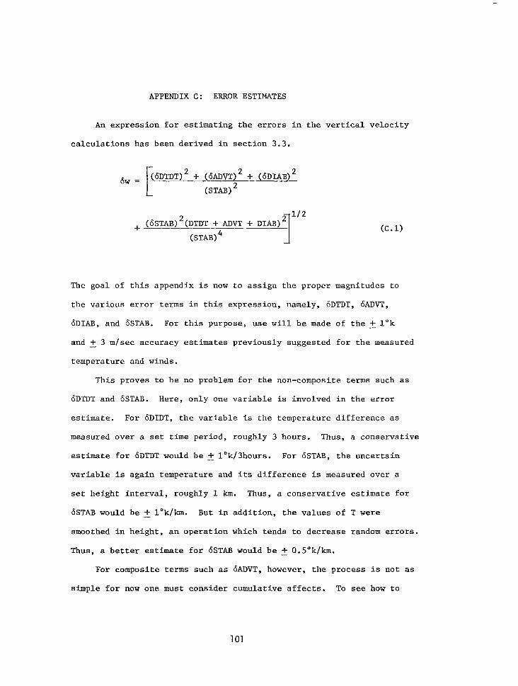
APPENDIX C: ERROR ESTIMATES

An expression for estimating the errors in the vertical velocity

calculations has been derived in section 3.3.

+ (GSTAB)~(DTDT + ADVT + DIAB)~ 1 l/2

(sTAB)~ (C.1)

The goal of this appendix is now to assign the proper magnitudes to

the various error terms in this expression, namely, 6DTDT, AADVT,

&DUB, and &TAB. For this purpose, use will be made of the +lOk

and + 3 m/set accuracy estimates previously suggested for the measured

temperature and winds.

This proves to be no problem for the non-composite terms such as

GDTDT and &TAB. Here, only one variable is involved in the error

estimate. For ADTDT, the variable is the temperature difference as

measured over a set time period, roughly 3 hours. Thus, a conservative

estimate for GDTDT would be + l"kj3hours. -- For &STAB, the uncertain

variable is again temperature and its difference is measured over a

set height interval, roughly 1 km. Thus, a conservative estimate for

&STAB would be + l'k/lon. But in addition, the values of T were

smoothed in height, an operation which tends to decrease random errors.

Thus, a better estimate for 6STAB would be rf: 0.5Ok/km.

For composite terms such as &NT, however, the process is not as

simple for now one must consider cumulative affects. To see how to

101

approach this problem, consider the complete advection term.

av ADVT = F (yH x 2) - l VVH> cc.21

The f -irst term on the right may be rewritten as follows:

Isin0) cc.31

where 0 is the angle between vH av

and -H . a, Expanding this into an

expression for relative error as in section 3.2, one obtains

6 (ADvT)~

(ADVT)l = cc.41

This form suggests the use of a percentage error for the various

terms. Physically, this would portray the situation where the mag-

nitude of the error increases as the magnitude of the various terms

increase. In fact, this is normally the case when calculating hori-

zontal advection terms. The percentage error approach will thus be

followed for the advection terms.

The accuracy estimate for wind measurements was given as + 3 m/set -

which is roughly 10% of the mean magnitude of the wind for this case.

Using this value, a conservative estimate for 6V, and &/$I would be

(0.1) yH a!H and (0.1) c respectively. One can again use + l'k for 6T, -

but with a mean magnitude for T of 250"k, the percentage error becomes

negligible. Finally, a 10% error estimate will be chosen for 6lsinOl.

102

Adding all of this up in equation (C.4), one obtains

6 (ADVT)~ : 0.3 (ADVT)l (C.5)

A similar estimate as above would be obtained for the second term on

the right of equation (C.2). The third term on the right was neglected

via scaling arguments as being an order of magnitude smaller than the

other terms. Its contribution to the error should thus not exceed

10%. Considering all of the above estimates along with the fact that

the individual errors may contribute negatively to each other, it is

felt that 30% represents a reasonable estimate of the percentage error

in the advection term.

Finally, one must assign a proper magnitude for 6DIAB. This term

has already been discussed in section 2.2 where it was suggested that

the diabatic term should be accurate within 20%. Therefore, the value

for 6DIAB will be taken as 0.2 (DUB).

All of the error terms in equation (C.l) have now been assigned.

These values will be used to continue the discussion in section 3.2.

103

APPENDIX D: p -l/2 CURVE

The goal of this Appendix is to construct a p -l/2 density profile

for inclusion in figures 14 and 15. Since such a curve is to be compared

to the calculated magnitudes of w, p' l/2 one in essence must draw a (o )

curve where p' represents a scaling factor. The value of p' is

assigned by using the magnitudes of w in figure 14 along with standard

atmospheric values of p to solve the following expression:

(Qy2 = w P (D.1)

Three values of p' were calculated in this manner representing the 30,

40, and 50 km altitudes. The results are given below in Table 7.

TABLE 7: Values of p'

Height (km)

30

40

50

P (i3dcm31

1.84 x 1O-5

4.00 x 10 -6

1.03 x 10 -6 :

W (cm/see)

3

5

6.5 i

p' (gm/cm sec2>

16.57 x lO-5

9.9 x 10 -5

4.34 x lo-5

A characteristic value of p' was obtained by taking an average of the

above three calculated values.

-' = 10.30 x lo-5 P CD.21

This value of p' is then used in equation (D.l) along with the standard

atmospheric values of o to draw the hypothetical profile of w in

104

figure 14. The same value of p' is also used in the construction of

the curve for figure 15.

105

I I III I II 11111 I

APPENDIX E: FOURIER ANALYSIS

The results from tidal theory are presented in terms of the

diurnal, semidiurnal, etc., components and associated vertical wave-

lengths which make up the tidal solutions. Thus, in order to compare

the current results to tidal predictions, the derived vertical motions

must also be decomposed into their diurnal, semidiurnal, etc., compo-

nents and associated vertical wavelengths. This will be accomplished

through the techniques of Fourier analysis as applied to discrete data

sets (see, for example, Panofsky and Brier, 1968).

Inessence, the discrete data points are assumed to represent a

continuous periodic function. Thus function is then approximated by a

least squares fit in terms of a series of sines and cosines. For a

function of an arbitrary variable, x, the series may be written as

N/2 27rix f(x) =T+Z (aisinr i=l

+ bi cos L;Z)

where f represents the mean value of the function, N represents the

size of the data set, L represents the wavelength or period of the data

set (depending on whether one is referring to a time or space series),

(E.1)

and i represents the number of the harmonic. The coefficients ai and

bi are given by the following relationships:

N 2lTix a. 1 = $ 1 [f(xjj sin ~1 j=l

bi = $. ! [f(x)j 2Trix

j=l cos 71 .

(E.2)

(E.3)

106

The amplitude of each harmonic, Ci, is then given as follows:

2 l/2 Ci = (ai + bi ) . (g.4)

The above information is also commonly represented in terms of the

spectral energy per unit frequency interval, Si (also referred to as

the spectral estimate).

si = $ (ai + bi2)

Y , (S.5)

where y represents the unit frequency interval.

The particular computer routine which has been used for this

analysis is the subroutine Fourt for the fast Fourier transform. The

only major restriction to using this routine is that the data points

must be evenly spaced. For the derived time series of vertical motions,

this requirement is met only for Kourou and Ft. Sherman. Thus, time

series analysis is limited to these two stations. For the derived

height series of vertical motions, this requirement is met at all five

stations comprising the study.

For the present case of 8 data points in time (N = 8), the above

technique produces a maximum of 4 harmonics representing the diurnal

(24 hour), semidiurnal (12 hour), terdiurnal (8 hour), and quadiurnal

(6 hour) contributions to the vertical motion field. The amplitudes of

the diurnal and semidiurnal components (Cl and C2) for Kourou and Ft.

Sherman have been plotted versus height in figures 16 and 17.

For the present case of 32 data points in height (N = 32), the

above technique produces 16 harmonics representing the variation of

107

vertical motion with height. The spectral energy per unit frequency

interval for each of the 16 harmonics, S i, is plotted versus vertical

wavelength in figure 18 for each of the five stations comprising the

present study. The spectral energies plotted represent averages over

time for each individual station.

In using the above technique, the assumption is informally made

that the discrete number of data points can be represented fully in

terms of the N/2 harmonics. Unfortunately, in real life, this is not

the case. Harmonics of number greater than N/2, whether noise or real

signal, could be aliasing their energy back into the lower harmonics

while harmonics too large to be defined by the data set could appear

as trends in the data. If one is interested specifically in the N/2

harmonics identified in the Fourier analysis (as is the case when

comparing the current results to tidal predictions), then both of these

possible effects should be accounted for.

First considering the aliasing, this potential problem can be

alleviated somewhat by smoothing the data. For the height series, the

data has been smoothed over 2 km with a l-2-1 filter. As discussed in

section 3.1, however, smoothing of the time series is not a feasible

option considering its small size. Thus, aliasing must be considered

to be a potential contaminant to the time series results.

The problem of having trends in the data can be alleviated by

removing the trends via regression techniques. For the height series

of vertical velocities, a trend is quite evident and in fact approaches

the expected p -l/2 amplitude increase with height relationship. As a

first approximation to removing this trend, a linear trend has been

108

removed from the vertical motions: The decomposition presented in

figure 18 represent those results with the linear trend removed.

For the time series of vertical velocities, one must again deal

with the small size of the data set. With only 8 points making up

the diurnal period, an error of only one or two hours in the positioning

of the end points of this series could produce significant apparent

trends which would not be there if the data series were without these

errors. Inspection of the derived vertical velocity series showed that

this was indeed the case, with linear trends appearing due to the in-

complete size of the series. Thus, it was felt advisable not to remove

trends from the time series data. This decision is enhanced also by

the fact that the larger time scale features for the equatorial middle

atmosphere which could possibly affect 24 hour or less time periods

(Kelvin waves, Rossby-gravity waves) have theoretical amplitudes at

least an order of magnitude smaller than the derived vertical motions

for the present study (see Holton, 1975). It is felt that such

amplitudes could not possibly influence the present analysis. As a

final check of this decision, a comparison was made between the results

with and without the linear trend removal. The only differences found

could be explained satisfactorily as being within the uncertainty of

the analysis. Thus, the entire question of removing the linear trend

from the vertical motion time series becomes merely one of academic

interest for the present study and of no practical consequence.

109

REFERENCES

Chapman, Sydney, and R. S. Lindzen, 1970: Atmospheric Tides, Thermal and Gravitational. D. Reidel Publishing Co., Dordrecht, Holland, 200 pp.

Craig, Richard A., and M. A. Lateef, 1962: Vertical motion during the 1957 stratospheric warming. J. Geophys. Res., 67, 1839-1854.

Dutton, J. A., 1976: The Ceaseless Wind, An Introduction to the Theory of Atmospheric Motion. McGraw-Hill, Inc., 579 pp.

Forsythe, G. E., 1945: A generalization of the thermal wind equation to arbitrary horizontal flow. Bull. Amer. Meteor. Sot., 26, 371-375.

Groves, G. V., 1975: Diurnal and semidiurnal oscillations of the upper atmosphere derived from grenade experiments at Natal, Brazil. J. Atmos. Terr. Phys., 37, 1133-1138.

Holton, James R., 1975: The dynamic meteorology of the stratosphere and mesosphere. Meteorological Monographs, American Meteorological Society, Boston, 15, 216 pp.

Kao, S. K., and N. J. Lordi, 1977: Characteristics of the Motions, Turbulence Intensity, Diffusivity, Flux of Momentum and Sensible Heat in the Upper Atmosphere. Contractor Report, NASA CR-2782, National Aeronautics and Space Administration, Washington, D.C., 56 PP-

Kays, Marvin D., and Richard A. Craig, 1965: On the order of magnitude of large-scale vertical motions in the upper stratosphere. J. Geophys. Res., 70, 4453-4461.

Lindzen, R. S., 1967: Thermally driven diurnal tide in the atmosphere. Quart. J. Roy. Meteor. Sot., 93, 18-42.

Lindzen, R. S., and Siu-Shung Hong, 1974: Effects of mean winds and horizontal temperature gradients on solar and lunar semidiurnal tides in the atmosphere. J. Atmos. Sci., 31, 1421-1446.

Miller, Alvin J., 1970: A note on vertical motion analysis for the upper stratosphere. Mon. Wea. Rev., 98, 616-620.

Murgatroyd, R. J., and R. M. Goody, 1958: Sources and sinks of radiative energy from 30 to 90 km. Quart. J. Roy. Meteor. Sot., 84, 225-234.

Panofsky, H. A., 1946: Methods of computing vertical motion in the atmosphere. J. Meteor., 3, 45-49.

110

REFERENCES (Continued)

Panofsky, Hans A., and Glen W. Brier, 1968: Some Applications of Statistics to Meteorology. Earth and Mineral Sciences Continuing Education, College of Earth and Mineral Sciences, The Pennsylvania State University, University Park, Pennsylvania, 224 pp.

Quiroz, Roderick S., 1969: The warming of the upper stratosphere in February 1966 and the associated structure of the mesosphere. Mon. Wea. Rev., 97, 541-552.

Schmidlin, F. J., 1976: Diurnal Tidal Analysis in the Equatorial Stratosphere and Mesosphere. Paper presented at nineteenth meeting of COSPAR, Philadelphia.

Schmidlin, F. J., Y. Yamasaki, A. Motta, and S. Brynsztein, 1975:Diurnal Experiment Data Report, March 19-20, 1974. NASA SP-3095, National Aeronautics and Space Administration, Washington, D.C., 150 pp.

Staff, Upper Air Branch, National Weather Service, 1976: Svnoptic Analysis. 5. 2, and 0.4 mb Surfaces for July 1973 Through June 1974. NASA SP-3102, Joint NASA-NOAA Publication, National Aeronautics and Space Administration, Washington, D.C., 140 pp.

The following references were also found to be quite useful, but were not specifically noted in the text.

Dopplick, T. G., 1971: The energetics of the lower stratosphere including radiative effects. Quart. J. Roy. Meteor. Sot., 97, 209-237.

Groves, G. V., 1976: Review lecture, rocket studies of atmospheric tides. Proc. R. Sot. Lond. A., 351, 437-469.

Kreitzberg, Carl W., 1964: The Structure of Occlusions as Determined From Serial Ascents and Vertically Directed Radar. AFCRL-64-26, Meteorology Laboratory Project 8641, Air Force Cambridge Research Laboratories, Office of Aerospace Research, U. S. Air Force, 121 pp.

Miller, Alvin J., 1967: Note on vertical motion in the lower strato- sphere. Beitrage Zur Physik der Atmosphare, 40, 29-48.

Nastrom, G. D., and A. D. Belmont, 1976: Diurnal stratospheric tide in meridional wind, 30 to 60 km, by season. J. Atmos. Sci., 33, 315-320.

111

1. Report No. .-

2. Government Accession No.

NASA CR-3096 -. ._ 4. Title and Subtitle

Vertical Motions in the Equatorial Middle Atmosphere

3. Recipient’s Catalog No.

5. Report Date April 1979

6. Performing Organization Code

--

7. Author(s)

Morris Larry Weisman

9. Performing Organization Name and Address

The Pennsylvania State University Department of Meteorology University Park, PA 16802

12. Sponsoring Agency Name and Address

National Aeronautics and Space Administration Wallops Flight Center Wallops Island, VA 23337

8. Performing Organization Report NO.

10. Work Unit No.

11. Contract or Grant No. NAS6-2726

13. Type of Report and Period Covered

Final Report

14. Sponsoring Agency Code

15. Supplementary Notes

16. Abstract

The stratospheric and mesospheric diurnal experiment of March 19, 20, 1974 offers a unique oppor- tunity to calculate and study small time scale vertical motions in the equatorial middle atmosphere. Since, however, the constraints of working in this region (data sparsity, lack of geostrophy, etc.) do not permit the use of standard vertical velocity calculation and analysis techniques, alternate techniques must be developed. As such, a single station vertical velocity equation which considers ageostrophic and diabatic effects is derived from the first law of thermodynamics and a generalized thermal wind relation. In addition, an analysis and verification procedure is developed which accounts for measurement and calculation errors as well as time and space continuity arguments and theoretical predictions.

This scheme is used to calculate vertical velocities at every kilometer between 25 and 60 km and for approximately every three hours for the above diurnal period at Kourou (French Guiana), Fort Sherman (Panama Canal Zone), Ascension Island, Antigua (British West Indies) and Natal (Brazil). The results, plotted as time series cross sections, suggest vertical motions ranging in magnitude from 1 or 2 cm/set at 30 km to as much as 15 cm/set at 60 km. The patterns depicted in the cross sections suggest the existence of internal gravity type waves in the motion field with diurnal, semidiurnal, and terdiurnal periods and vertical wavelengths between Ip,tnd 30 km. There is also evidence of a 20-50 km/day downward phase progression and a (density) amplitude increase with height relationship as is often suggested for such motions.

It is found that many of the general features of the results agree well with atmospheric tidal predictions (Lindzen, 1967, Lindzen and Hong, 1974) but many particular features suggest that both smaller time scale gravity waves (periods < 6 hours) and synoptic type waves (periods > 1 day) may be interacting significantly with the tidal fields. This suggests that more research is needed to help delineate the types and scales of motion which make up this region of the atmosphere.

Overall, the results suggest that vertical motions can be calculated for the equatorial middle atmosphere and must be considered a significant part of the motion for time scales from 8 to 24 hours.

17. Key Words (Suggested by Author(s))

Sounding Rockets Atmospheric Tides Meteorology Wind (Meteorology) Vertical Motion Stratosphere Tidal Oscillation

18. Distribution Statement

Unclassified - Unlimited

STAR Category 47

19. Security Classif. (of this report) 20. Security Classif. (of this page)

Unclassified Unclassified

21. No. of Pages

111

22. Rice’

$6.50

*For sale by the National Technical Information Service, Springfield, Virginia 22151