601.465/665 — Natural Language ProcessingHomework 3: Smoothed Language Modeling

Prof. Jason Eisner — Fall 2021Due date: Sunday 10 October, 11 pm

Probabilistic models are an indispensable part of modern NLP. This homework will try to convinceyou that even simplistic and linguistically stupid models like n-gram models can be useful, provided theirparameters are estimated carefully. See section A in the reading below.

You now know enough about probability to build and use some trigram language models. You will ex-periment with different types of smoothing, including using PyTorch to train a log-linear model. You willalso get some experience in running corpus experiments over training, development, and test sets. This isthe only homework in the course to focus on that.

Homework goals: After completing this homework, you should be comfortable with• estimating conditional probabilities from supervised data

– direct estimation of probabilities (with simple or backoff smoothing)– conditional log-linear modeling (including feature engineering using external information such

as lexicons)– subtleties of language modeling (tokenization, EOS, OOV, OOL)– subtleties of training (logarithms, autodiff, SGD, regularization)

• evaluating language models via sampling, perplexity, and multiple tasks, using a train/dev/test split• tuning hyperparameters by hand to improve a formal evaluation metric• implementing these methods cleanly in Python

– partitioning the work sensibly into different classes, files, and scripts that play nicely together– using basic facilities of PyTorch

Collaboration: You may work in teams of up to 2 on this homework. That is, if you choose, you maycollaborate with 1 partner from the class, handing in a single homework with multiple names on it. You areexpected to do the work together, not divide it up: if you didn’t work on a question, you don’t deserve creditfor it! Your solutions should emerge from collaborative real-time discussions with both of you present. Yourcollaborator may not be your discussion partner from HW2. Make new friends! :-)

Reading: Read the long handout attached to the end of this homework!

Materials: Python starter code and data are at http://cs.jhu.edu/˜jason/465/hw-lm/. You’vealready used some of the data (the lexicons) in the previous homework.1

1If you lack the bandwidth to download all of the data files to your own machine, just download a few. Once your code isworking, you can upload your code to the ugrad filesystem and run it on one of the ugrad machines, where the same files areavailable in the directory /usr/local/data/cs465/hw-lm/. Please don’t make additional copies of the data on the ugradfilesystem, as this would waste space; you can use symbolic links instead.

On getting programming help: Use Python, building on the provided starter code. Since this is an upper-level NLP class, not a programming class, I don’t want you wasting much time on low-level issues likesyntax, type annotations, and I/O. Also, I don’t want you to get stuck on understanding the starter code. Byall means seek help from someone who knows the language better! Your responsibility is the NLP stuff—you do have to design, write, and debug the interesting code and data structures on your own. But I don’tconsider it cheating if another hacker (or a CA) helps you with Python issues. Those aren’t InterestingTM.

How to hand in your written work: Via Gradescope as before. Besides the comments you embed inyour source code, put all other notes, documentation, and answers to questions in a PDF file.

The� symbol in the left margin of this handout marks items that should be answered in your PDF. Inyour PDF, you should refer to question numbers like 3(a). (Don’t refer to the blue� numbers; they are justfor your convenience and may change if this homework handout is updated.)

How to test and hand in your code and models:

• Your code and your trained models will need to be zipped and uploaded separately on Gradescope.�1

We will post more detailed instructions on Piazza.

• For the parts where we tell you exactly what to do, an autograder will check that you got it right.

• For the open-ended challenge (question 7(d)), an autograder will run your system and score its accu-racy on test and grading-test data.

– You should get a decent grade if you do at least as well as the “baseline” system provided by theTAs. Better systems will get higher grades.

– The test results are intended to help you develop your system. Grades will be based on thegrading-test data that you have never seen.

1 Perplexities and corpora

Your starting point is the sample programs build vocab.py build lm.py fileprob.py, inthe code directory. The INSTRUCTIONS file in the same directory explains how to get the programsrunning. Those instructions will let you automatically compute the log2-probability of three sample files(data/speech/{sample1,sample2,sample3}). Try it!

More precisely, for each file, fileprob will give you the total log2-probability of all token sequencesin the file. Each line of the file is considered to be a separate token sequence (sentence or document) that isimplicitly preceded by BOS and followed by EOS.

Next, you should spend a little while looking at those sample files yourself, and in general, browsingaround the data/ directory to see what’s there. See reading sections B and C for more information.

If a language model is built from the data/speech/switchboard-small corpus, using add-0.01�2

smoothing, what is the model’s perplexity per word on each of the three sample files? (You can computethis from the log2-probability that fileprob prints out, as discussed in class and in the recommendedtextbooks. Use the command wc -w on a file to find out how many word tokens it contains. But this willnot count the EOS at the end of each line, so also add the number of lines, which is computed by wc -l.)

What happens to the log2-probabilities and perplexities if you train instead on the larger switchboard�3

corpus? Why?

2

2 Implementing a generic text classifier

Modify fileprob to obtain a new program textcat that does text categorization via Bayes’ Theorem.The two programs both use the same probs module to get the language model probabilities. So when

you extend probs.pywith new smoothing methods in question 5 below, they will immediately be availablefrom both programs.

textcat should be run from the command line almost exactly like fileprob. However,

• it needs to take two language models, one for each category of text• it needs to specify the prior probability of the first category

Of course, you can imagine extending this to do n-way classification, with n language models eachtrained on a different corpus, and prior probabilities for each of the n categories. But in this homework, wewill stick with binary classification.

Again, consult INSTRUCTIONS for some tips on working with the starter code.You’ll train models of genuine emails (gen) and spam emails (spam). You (and the graders) should

then be able to use your program for classification like this:

./textcat.py gen.model spam.model 0.7 foo.txt bar.txt baz.txt

which uses the two trained models to classify the listed files. Its printed output should label each file with atraining corpus name (in this case gen or spam):

spam.model foo.txtspam.model bar.txtgen.model baz.txt1 files were more probably gen.model (33.33%)2 files were more probably spam.model (66.67%)

In other words, your program classifies each file by printing its maximum a posteriori class (the file nameof the model that more probably generated it). Then it prints a summary of all the files.

The number 0.7 on the above command line specifies your prior probability that a test file will be gen.Thus, 0.3 is your prior probability that it will be spam. See reading section C.2.

Please use the exact output formats above. If you would like to print any additional output lines for yourown use, please direct it to STDERR, using the logging facility as illustrated in the starter code.

As reading section D.3 explains, both language models that you provide to textcat should use thesame finite vocabulary. Specifically, please construct this vocabulary to consist of words that appeared ≥ 3times in the union of the gen and spam training corpora, plus OOV and EOS.2

3 Evaluating a text classifier

In this question, you will evaluate your textcat program on the problem of spam detection. The datasetsare under data/gen spam. Look at the README file there, and then examine the training data to get asense for how the genuine emails differ from the spam emails. (Don’t peek at the test data!)

2Of course, OOV and EOS may appear in the training corpora too—in fact, EOS must appear. But they might appear < 3 times.build vocab is careful to include them in the vocabulary anyway. This is important. If OOV weren’t in the vocabulary, wewouldn’t be able to handle OOV words. And if EOS weren’t in the vocabulary (and hence was treated as just part of the OOVcategory), then we couldn’t sample from the language model—we wouldn’t know when we had generated EOS and could end thesentence!

3

Using add-1 smoothing, run textcat on all the dev data for your chosen task. That is, train yourlanguage models on the gen and spam training sets, and then classify the files gen spam/dev/gen/*and gen spam/dev/spam/*. Use 0.7 as your prior probability of gen.

(a) From the results, you should be able to compute a total error rate for the technique. That is, what�4

percentage of the dev files were classified incorrectly?

(b) Extra credit: We will focus on the spam detection problem in this assignment. But lectures in class,5

focused on the language identification task, using a character-trigram model instead of a word-trigrammodel. Formally, these settings are very similar. If you’re curious, you can try out the language ID set-ting as well, using the data in data/english spanish. This should be quite fast since the corporaand vocabulary are small. Train your language models on the en.1K and sp.1K datasets, then clas-sify the files english spanish/dev/english/*/* and english spanish/dev/spanish/*/*.Use 0.7 as your prior probability of English. All of these files have been tokenized into characters foryou, so that you can use the same code as before.3

What percentage of the dev files were classified incorrectly?

(c) How small do you have to make the prior probability of gen before textcat classifies all the dev�6

files as spam?

(d) Now try add-λ smoothing for λ 6= 1. First, use fileprob to experiment by hand with differentvalues of λ > 0. (You’ll be asked to discuss in question 4(b) why λ = 0 probably won’t work well.)

What is the minimum cross-entropy per token that you can achieve on the gen development files�7

(when estimating a model from gen training files with add-λ smoothing)? How about for spam?

(e) In principle, you should apply different amounts of smoothing to the gen and spam models. Forexample, if gen’s dev set has a higher rate of novel words than spam’s dev set, then you’d want tosmooth gen more.

However, for simplicity in this homework, let’s smooth both models in exactly the same way. So what�8

is the minimum cross-entropy per token that you can achieve on all development files together, if bothmodels are smoothed with the same λ?

(As in the previous question, you should be evaluating the gen model on gen development files only,and the spam model on spam development files only, to make sure that they are good models oftheir intended categories. To measure the overall cross-entropy per token for a given λ, find the totalnumber of bits that it takes to predict all of the development files from their respective models. Thismeans running fileprob twice: once for the gen data and once for the spam data. Add the tworesults, and then divide by the total number of tokens in all of the development files.)

What value of λ gave you this minimum cross-entropy? Call this λ∗. (See reading section E for why�9

you are using cross-entropy to select λ∗.)

(f) Each of the dev files has a length. The length in words is embedded in the filename (as the firstnumber).

3Properly speaking, these sequences are not complete sentences. They are substrings plucked from the middle of documents, sothey don’t really have BOS or EOS. Ideally, you would change the iterator over trigrams to reflect that: if you observe the sequencew1w2w3w4w5, the only trigram probabilities that you can compute or train are p(w3 | w1w2), p(w4 | w2w3), and p(w5 | w3w4),because you don’t know what was before w1 (not necessarily BOS) or after w5 (not necessarily EOS).

4

Come up with some way to quantify or graph the relation (on dev data) between file length andthe classification accuracy of add-λ∗. Some tips about graphing are in http://cs.jhu.edu/

˜jason/465/hw-lm/graphing.html. You may also be interested in correlations.

Write up your results.�10

(g) Extra credit: If you are also experimenting with language ID, similarly report on the relation (on dev,11

data) between file length and classification accuracy. The length in words is again embedded in thefilename (as the first number), and also appears in the directory name.

(h) Now try increasing the amount of training data. (Keep using add-λ∗, for simplicity.) Compute theoverall error rate on dev data for training sets of different sizes: gen vs. spam; gen-times2 vs.spam-times2 (twice as much training data); and similarly for . . .-times4 and . . .-times8.

Graph the training size versus classification accuracy. This is sometimes called a “learning curve.”�12

Do you expect accuracy to approach 100% as training size→∞?

(i) Extra credit: If you’re also experimenting with language ID, you can do the same exercise there if,13

you’re still curious. We’ve provided training corpora of 6 sizes: en.1K vs. sp.1K (1000 characterseach); en.2K vs. sp.2K (2000 characters each); and similarly for 5K, 10K, 20K, and 50K.

4 Analysis

Reading section F gives an overview of several smoothing techniques beyond add-λ.

(a) At the end of question 2, V was carefully defined to include OOV. So if you saw 19,999 differentword types in training data, then V = 20, 000. What would go wrong with the UNIFORM estimate if�14

you mistakenly took V = 19, 999? What would go wrong with the add-λ estimate?

(b) What would go wrong with the add-λ estimate if we set λ = 0? (Remark: This gives an unsmoothed�15

“relative frequency estimate.” It is commonly called the maximum-likelihood estimate, because itmaximizes the probability of the training corpus.)

(c) Let’s see on paper how backoff behaves with novel trigrams. If c(xyz) = c(xyz′) = 0, then does�16

it follow that p(z | xy) = p(z′ | xy) when those probabilities are estimated by smoothing? In youranswer, work out and state the value of p(z | xy) in this case. How do these answers change ifc(xyz) = c(xyz′) = 1?

(d) In add-λ smoothing with backoff, how does increasing λ affect the probability estimates? (Think�17

about your answer to the previous question.)

5 Backoff smoothing

Implement add-λ smoothing with backoff, as described in reading section F.3. This should be just a fewlines of code. You will only need to understand how to look up counts in the hash tables. Just study how theexisting methods do it.

Hint: So p(z | xy) should back off to p(z | y), which should back off to p(z), which backs off to. . . what?? Figure it out! Think back to the Tablish language from recitation.

5

You will submit trained add-λ∗ models as in question 3(e). For simplicity, just use the same λ∗ as inthat question, even though some other λ might work better with backoff.

Note: To check that you are smoothing correctly, the autograder will run your code on small trainingand testing files.

6 Sampling from language models

So far, we have used our language models to compute the probability of given word sequences. Eachlanguage model represents a probability distribution over word sequences.

But because these are well-defined probabilistic models, we can also sample from the distributions theyrepresent. As we saw in class, we sample random text by rolling a sequence of weighted dice whose sidesare words. This is a good way to see what the language model does and doesn’t know about English.

This is just like Homework 1, where your PCFG allowed you both to sample a new sentence (randsent)and to compute the probability of a given sentence (parse). You can also do both of these things with ann-gram model, which is a different generative model of text.4

Implement a generic sampling method that will work with any of our trained language models. When�18

called, the function should condition on BOS and produce new tokens until it reaches EOS. These tokensare drawn from the smoothed model distribution according to their probabilities. This should remind you ofrandsent in Homework 1.

Write a separate script based on fileprob that will sample k sentences from a given language model,using the sampling method you described above. (Especially because of UNIFORM, impose a maximumlength limit M , as in the PCFG homework. Sequences longer than your configurable limit should be trun-cated with “...”.)

We should be able to call your script like this:

./trigram_randsent.py model_file 10 --max_length 20

Choose two trained models that seem to have noticeably different behavior. (They might use different�19

smoothing methods, or different hyperparameters.) Give a sample of 10 sentences from each of the models.Discuss the differences you see and why they arise.

7 Implementing a log-linear model and training it with backpropagation

(a) Add support for a log-linear trigram model. This is another smoothed trigram model, but the smooth-ing comes from several feature functions instead of modified or backed-off counts. As usual, seeINSTRUCTIONS for details about working with the starter code.

Your code will need to compute p(z | xy) using the specific features in reading section F.4.1. Theparameters ~θ will be stored in X and Y matrices. You can use random or zero parameters at first, justto get the code working.

Remember that you need to look up an embedding for each word, falling back to the OOL embeddingif that word is not in the lexicon. In particular, OOV will fall back to OOL.

You can use embeddings of your choice from the lexicons directory. (See the README file in thatdirectory. Make sure to use word embeddings for gen/spam, but character embeddings if you try

4Actually, not so different: an n-gram model turns out to be a special case of a PCFG. Can you show that this is true for n = 2?

6

english/spanish.) These word embeddings were derived from Wikipedia, a large diverse corpuswith lots of useful evidence about the usage of many English words.

(b) Implement a function that uses stochastic gradient descent to find the X and Y matrices that mini-mize −F (~θ), which is the L2-regularized objective function described in reading section H.1. (Thisis equivalent to maximizing F (~θ).)

You may prefer to try this out first on language ID (data/english spanish), since training alog-linear model takes significantly more time than add-λ smoothing. For example, here’s what youshould get if you train a log-linear language model on en.1K, with a vocabulary of size 30 derivedfrom en.1K with threshold 3, the features described in reading section F.4, the character embeddingsof dimension d = 10 (chars-10.txt), regularization strength C = 1, and the ConvergentSGDoptimization described in reading section I.8.1:

Training from corpus en.1Kepoch 1: F = -3.2339084148406982epoch 2: F = -3.109910249710083epoch 3: F = -3.0625805854797363

... [you should print these epochs too]epoch 10: F = -2.967740774154663Finished training on 1027 tokens

For the autograder’s sake, when log linear is specified on the command line, please train for E =10 epochs, use the exact hyperparameters suggested in reading section I.5, use ConvergentSGD,and print output in the format above (this is printing F (~θ) rather than Fi(~θ)). We won’t expect you tomatch the numbers exactly, but your numbers should be somewhat close.

(c) You should now be able to measure cross-entropies and text categorization error rates under yourfancy new language model! textcat should work as before. Just construct two log-linear modelsover a shared vocabulary, and then compare the probabilities of a new document (dev or test) underthese models.

Report cross-entropy and text categorization accuracy on gen spam withC = 1, but also experiment�20

with other values of C > 0, including a small value such as C = 0.05. Let C∗ be the best value youfind. Using C = C∗, play with different embedding dimensions and report the results. How andwhen did you use the training, development, and test data? What did you find? How do your resultscompare to add-λ backoff smoothing?

(d) Now you get to have some fun! Add some new features to the log-linear model and report the effect on�21

its performance. Some possible features are suggested in reading section J. You should make at leastone non-trivial improvement; you can do more for extra credit, including varying hyperparametersand training protocols (reading sections I.5 and I.8).

A good way to devise features is to try sampling sentences from the basic log-linear model (usingyour sample method from question 6). What’s wrong with these sentences? Specifically, what’swrong with the trigrams, since that’s all that you can fix within the limits of a trigram model? Arethere features that you think are too frequent, or not frequent enough? If so, try adding these features,and then the trained model should get them to occur at the right rate. (Remember from the log-linearvisualization that the predictions of a log-linear model, if it was trained without regularization, willhave the same features on average as actual words in the training corpus.)

7

Your improved method should be selected with the command-line argument log linear improved(in place of add lambda, log linear, etc.). You will submit your code and your trained modelto Gradescope for autograding.

You are free to submit many versions of your system—with different implementations of log linear improved.All will show up on the leaderboard, with comments, so that you and your classmates can see whatworks well. For final grading, the autograder will take the submitted version of your system thatworked best on the released test data, and then evaluate its performance on grading-test data.

8 Speech recognition

Finally, we turn briefly to speech recognition. In this task, instead of choosing the best model for a givenstring, you will choose the best string for a given model.

The data are in the speech subdirectory, drawn from the Switchboard corpus (see the README filethere). As usual, it is divided into training, development, and test sets. Here is a sample file (dev/easy/easy025):8 i found that to be %hesitation very helpful0.375 -3524.81656881726 8 i found that the uh it’s very helpful0.250 -3517.43670278477 9 i i found that to be a very helpful0.125 -3517.19721540798 8 i found that to be a very helpful0.375 -3524.07213817617 9 oh i found out to be a very helpful0.375 -3521.50317920669 9 i i’ve found out to be a very helpful0.375 -3525.89570470785 9 but i found out to be a very helpful0.250 -3515.75259677371 8 i’ve found that to be a very helpful0.125 -3517.19721540798 8 i found that to be a very helpful0.500 -3513.58278343221 7 i’ve found that’s be a very helpful

Each file has 10 lines and represents a single audio-recorded utterance U . The first line of the file is thecorrect transcription, preceded by its length in words. The remaining 9 lines are some of the possible tran-scriptions that were considered by a speech recognition system—including the one that the system actuallychose to output. Let’s reason about how to choose among the 9 candidates.

Consider the last line of the sample file. The line shows a 7-word transcription ~w surrounded by sentencedelimiters <s>. . .</s> and preceded by its length, namely 7. The number −3513.58 was the speechrecognizer’s estimate of log2 p(U | ~w): that is, if someone really were trying to say ~w, what is the log-probability that it would have come out of their mouth sounding like U?5 Finally, 0.500 = 4

8 is the worderror rate of this transcription, which had 4 errors against the 8-word true transcription on the first line ofthe file; this will be used in question 9 below.6

We won’t actually make you write any code here. But according to Bayes’ Theorem, how should you�22

choose among the 9 candidates? That is, what quantity are you trying to maximize, and how should youcompute it?

(Hint: You want to pick a candidate that both looks like English and looks like the audio utterance U .Your trigram model tells you about the former, and −3513.58 is an estimate of the latter.)

5Actually, the real estimate was 15 times as large. Noisy-channel speech recognizers are really rather bad at estimating log p(U |~w), so they all use a horrible hack of dividing this value by about 15 to prevent it from influencing the choice of transcription toomuch! But for the sake of this question, just pretend that no hack was necessary and−3513.58 was the actual value of log2 p(U | ~w)as stated above.

6The word error rate of each transcription was computed for you by a scoring program, or “scorer.” The correct transcriptionon the first line sometimes contains special notation that the scorer paid attention to. For example, %hesitation on the first linetold the scorer to count either uh or um as correct.

8

9 Extra credit: Language modeling for speech recognition

Actually implement the speech recognition selection method in question 8, using one of the language modelsyou’ve already built. Use the switchboard corpus for training. You may experiment on the developmentset before getting your final results from the test set. When experimenting, you may want to start out withtraining on switchboard-small, just for speed.

(a) Modify fileprob to obtain a new program speechrec that chooses this best candidate. As usual,see INSTRUCTIONS for details.

The program should look at each utterance file listed on the command line, choose one of the 9 tran-scriptions according to Bayes’ Theorem, and report the word error rate of that transcription (as givenin the first column). Finally, it should summarize the overall word error rate over all the utterances—the total number of errors divided by the total number of words in the correct transcriptions.

Of course, the program is not allowed to cheat: when choosing the transcription, it must ignore eachfile’s first row and first column!

Sample input (please allow this format):

./speechrec switchboard_whatever.model easy025 easy034

Sample output (please use this format—but you are not required to get the same numbers):

0.125 easy0250.037 easy0340.057 OVERALL

Notice that the overall error rate 0.057 is not an equal average of 0.125 and 0.037; this is becauseeasy034 is a longer utterance and counts more heavily.

Hints about how to read the file:

• For all lines but the first, you should read a few numbers, and then as many words as theinteger told you to read (plus 2 for <s> and </s>). Alternatively, you could read the wholeline at once and break it up into an array of whitespace-delimited strings.

• For the first line, you should read the initial integer, then read the rest of the line. The restof the line is only there for your interest, so you can throw it away. The scorer has alreadyconsidered the first line when computing the scores that start each remaining line.Warning: For the first line, the notational conventions are bizarre, so in this case the initialinteger does not necessarily tell you how many whitespace-delimited words are on the line.Thus, just throw away the rest of the line! (If necessary, read and discard characters up throughthe end-of-line symbol \n.)

(b) What is your program’s overall error rate on the carefully chosen utterances in test/easy? How,23

about on the random sample of utterances in test/unrestricted?

To get your answer, you need to choose a smoothing method, so pick one that seems to work well onthe development data dev/easy and dev/unrestricted. Be sure to tell us which method you,24

picked and why! What would be an unfair way to choose a smoothing method?

9

10 Extra credit: Open-vocabulary modeling

We have been assuming a finite vocabulary by replacing all unknown words with a special OOV symbol. Butan alternative is an open-vocabulary language model (reading section D.5).

Devise a sensible way to estimate the word trigram probability p(z | xy) by backing off to a lettern-gram model of z if z is an unknown word. Also describe how you would train the letter n-gram model.

Just giving the formulas for your estimator will get you some extra credit. Implementing and testing,25

them would be even better!Notes:

• x and/or y and/or z may be unknown; be sure you make sensible estimates of p(z | xy) in all thesecases

• be sure that∑

z p(z | xy) = 1

10

601.465/665 — Natural Language ProcessingReading for Homework 3: Smoothed Language Modeling

Prof. Jason Eisner — Fall 2021

We don’t have a required textbook for this course. Instead, handouts like this one are the main readings.This handout accompanies homework 3, which refers to it.

A Are n-gram models useful?

Why build n-gram models when we know they are a poor linguistic theory? Answer: A linguistic systemwithout statistics is often fragile, and may break when run on real data. It will also be unable to resolveambiguities. So our first priority is to get some numbers into the system somehow. An n-gram model is astarting point, and may get reasonable results even though it doesn’t have any real linguistics yet.

Speech recognition. Speech recognition systems made heavy use of trigram models for decades. Alter-native approaches that don’t look at the trigrams do worse. One can do better by building fancy languagemodels that combine trigrams with syntax, topic, and so on. But for a long time, you could only do a littlebetter—dramatic improvements over trigram models were hard to get. In the language modeling commu-nity, a rule of thumb was that you had enough for a Ph.D. dissertation if you had managed to reduce a goodtrigram model’s perplexity per word by 10% (equivalent to reducing the cross-entropy by just 0.152 bits perword).

Machine translation. Statistical machine translation (MT) systems were originally developed in the late1980’s and made use of trigram language models. After a quiet period, this paradigm was resurrected at theend of the century and started getting good practical results. Statistical MT systems often included 5-grammodels trained on massive amounts of data.

Why 5-grams? Because an MT system that translates into English has to generate a new fluent sentenceof English, and 5-grams do a better job than 3-grams of memorizing common phrases and local grammaticalphenomena.

An English speech recognition system can get away without 5-grams because it is not generating a newEnglish sentence. It observes the spoken version of an existing English sentence, and only has to guess whatwords the speaker actually said. A 3-gram model helps to choose between “flower,” “flour,” and “floor” byusing one word of context on either side. That already provides most of the value that we can get out of localcontext. Going to a 5-gram model wouldn’t help too much with this choice, because it still wouldn’t look atenough of the sentence to determine whether we’re talking about gardening (“flower”), baking (“flour”), orcleaning (“floor”).

R-1

Smoothing. Fancy smoothing techniques developed in the 1990’s, applied to trigram models, eventuallymanaged to achieve up to a total 50% reduction in perplexity per English word (equivalent to a cross-entropyreduction of 1 bit per word). A thorough review supported by careful comparative experiments can be foundin Goodman (2001).

As they noted, however, improving perplexity didn’t reliably improve the error rate of the speech recog-nizer. In some sense, the speech recognizer only needs the language model to break ties among utterancesthat sound similar. Many improvements to perplexity didn’t happen to help break these ties.

Neural language models. A line of work starting in 2000 used neural networks to produce smoothed prob-abilities for n-gram language models. These neural networks can be thought of as log-nonlinear models—ageneralization of the log-linear models considered in reading section F.4 below. The starting point for bothis the word embeddings that were introduced on the previous homework.

Next, recurrent neural networks (RNNs) became a popular way to get beyond n-gram models. We willtouch on these methods in this course. They are not limited to a fixed-length history. They can learn toexploit complex patterns in which the choice of next word is affected by the syntax, semantics, topic, style,and format of the left context.

RNN-based language models were originally proposed in 1991 by the inventor of RNNs, but there seemto be no published results on real data until 2010. In general, neural networks played little role in practicalNLP until about 2014. Around then, thanks to a series of small innovations over the preceding decade inneural network architectures and parameter optimization, together with larger datasets and faster hardware,neural methods in NLP started to show real gains over traditional non-neural probabilistic methods. Inparticular, neural language models started to show real gains over n-gram models. However, it was notedthat cleverly smoothed 7-gram models could still do about as well as an RNN model by looking at lots offeatures of the previous 6-gram (Pelemans et al. (2016)).

In the later half of the 2010s, a new neural architecture called the Transformer showed further empiricalgains in language modeling, halving perplexity (i.e., saving 1 bit of cross-entropy) over RNN models ofcomparable size.

More training data. Of course, training on larger corpora helps any method! As of 2020, the largestpublicly announced language model, GPT-3 (Brown et al., 2020), is an enormous Transformer with 175billion parameters, trained on 500 billion tokens1 of (mostly) English text obtained by crawling the web. Itachieves a perplexity of 20.5 on the Penn Treebank test set and is quite remarkably good at generating andextending text passages across a wide range of topics, styles, and formatting. Its creators showed that theseabilities can be used to help solve many other NLP tasks, because the language model has to know a lotabout language, meaning, and the real world in order to do such a good job of predicting what people aregoing to say next.

B Boundary symbols

Remember from the previous homework that a language model estimates the probability of any word se-quence ~w. In a trigram model, we use the chain rule and backoff to assume that

p(~w) =

N∏i=1

p(wi | wi−2, wi−1)

1These tokens are actually word fragments, rather than words: see reading section D.6.

R-2

with start and end boundary symbols handled as in the previous homework.In other words, wN = EOS (“end of sequence”), while for i < 1, wi = BOS (“beginning of sequence”).

Thus, ~w consists of N − 1 words plus an EOS symbol. Notice that we do not generate BOS but we docondition on it (it was always there).2 Conversely, we do generate EOS but never condition on it (nothingfollows it). The boundary symbols BOS, EOS are special symbols that do not appear among w1 . . . wN−1.

In the homework that accompanies this reading, we will consider every line in a file to implicitly bepreceded by BOS and followed by EOS. A file might be a sentence, or an email message, or a text fragment.

C Datasets for Homework 3

Homework 3 will mention corpora for three tasks: spam detection, language identification, and speechrecognition. They are all at http://cs.jhu.edu/˜jason/465/hw-lm/data/. Each corpus has aREADME file that you should look at.

C.1 The train/dev/test split

Each corpus has already been divided for you into training, development, and test sets, which are in separatedirectories. You will collect counts on train, tune the “hyperparameters” like λ to maximize performanceon dev, and then evaluate your performance on test.

In principle, you shouldn’t look at test until you’re ready to get the final results for a system, and thenyou must commit to reporting those results to avoid selective reporting. The danger of experimenting ontest to improve performance on test is that you might “overfit” to it—that is, you might find your wayto a method that seems really good, but is actually only good for that particular test set, not in general.

To be on the safe side, we will actually evaluate your system in a blind test, when we run it on new datayou’ve never seen. Your grade will therefore be determined based on a grading-test set that you don’thave access to. So overfitting to test might give you good results on test in your writeup, but it will hurtyou on grading-test. (Just as if you tell your boss that the system works great and is ready to ship, andthen it doesn’t work for real users.)

C.2 Class ratios

In the homework, you’ll have to specify a prior probability that a file will be genuine email (rather thanspam) or English (rather than Spanish). In other words, how often do you expect the real world to producegenuine email or English in your test data? We will ask you to guess 0.7.

Of course, your system won’t know the true fraction on test data, because it doesn’t know the trueclasses—it is trying to predict them.

We can try to estimate the fraction from training data, or perhaps more appropriately from dev data(which are supposed to be “like the test data”). It happens that in dev data, 2

3 of the documents are genuineemail, and 1

2 are English. In this case, the prior probability is a parameter or hyperparameter of the model,to be estimated from training or dev data as usual.

But if you think that test data might have a different rate of spam or Spanish than training data, then theprior probability is not necessarily something that you should represent within the model and estimate fromtraining data. Instead it can be used to represent your personal guess about what you think test data will belike.

2Just like the ROOT symbol in a PCFG.

R-3

Indeed, in the homework, you’ll use training data only to get the smoothed language models, whichdefine the likelihood of the different classes. This leaves you free to specify your prior probability of theclasses on the command line. This setup would let you apply the system to different test datasets aboutwhich you have different prior beliefs—the spam-infested email account that you abandoned, versus yournew private email account that only your family knows about.

Does it seem strange to you that a guess or assumption might have a role in statistics? That is actuallycentral to the Bayesian view of statistics—which says that you can’t get something for nothing. Just as youcan’t get theorems without assuming axioms, you can’t get posterior probabilities without assuming priorprobabilities.

D The vocabulary

D.1 Choosing a finite vocabulary

All the smoothing methods assume a finite vocabulary, so that they can easily allocate probability to all thewords. But is this assumption justified? Aren’t there infinitely many potential words of English that mightshow up in a test corpus (like xyzzy and JacrobinsteinIndustries and fruitylicious)?

Yes there are . . . so we will force the vocabulary to be finite by a standard trick. Choose some fixed,finite vocabulary at the start. Then add one special symbol OOV that represents all other words. You shouldregard these other words as nothing more than variant spellings of the OOV symbol.

Note that OOV stands for “out of vocabulary,” not for “out of corpus,” so OOV words may have tokencount > 0 and in-vocabulary words may have count 0.

D.2 Consequences for evaluating a model

For example, when you are considering the test sentence

i saw snuffleupagus on the tv

what you will actually compute is the probability of

i saw OOV on the tv

which is really the total probability of all sentences of the form

i saw [some out-of-vocabulary word] on the tv

Admittedly, this total probability is higher than the probability of the particular sentence involving snuffleupagus.But in most of this homework, we only wish to compare the probability of the snuffleupagus sentence underdifferent models. Replacing snuffleupagus with OOV raises the sentence’s probability under all themodels at once, so it need not invalidate the comparison.3

D.3 Comparing apples to apples

We do have to make sure that if snuffleupagus is regarded as OOV by one model, then it is regardedas OOV by all the other models, too. It’s not appropriate to compare pmodel1(i saw OOV on the tv)

3Problem 10 explores a more elegant approach that may also work better for text categorization.

R-4

with pmodel2(i saw snuffleupagus on the tv), since the former is actually the total probabilityof many sentences, and so will tend to be larger.

So all the models must have the same finite vocabulary, chosen up front. In principle, this sharedvocabulary could be any list of words that you pick by any means, perhaps using some external dictionary.

Even if the context “OOV on” never appeared in the training corpus, the smoothing method is requiredto give a reasonable value anyway to p(the | OOV,on), for example by backing off to p(the | on).

Similarly, the smoothing method must give a reasonable (non-zero) probability to p(OOV | i,saw).Because we’re merging all out-of-vocabulary words into a single word OOV, we avoid having to decide howto split this probability among them.

D.4 How to choose the vocabulary

How should you choose the vocabulary? For this homework, simply take it to be the set of word types thatappeared ≥ 3 times anywhere in training data. Then augment this set with a special OOV symbol. Let Vbe the size of the resulting set (including OOV). Whenever you read a training or test word, you shouldimmediately convert it to OOV if it’s not in the vocabulary. This is fast to check if you store the vocabularyin a hash set.

To help you understand/debug your programs, we have grafted brackets onto all out-of-vocabulary wordsin one of the datasets (the speech directory, where the training data is assumed to be train/switchboard).This lets you identify such words at a glance. In this dataset, for example, we convert uncertain to[uncertain]—this doesn’t change its count, but does indicate that this is one of the words that yourcode will convert to OOV (if your code is correct).

D.5 Open-vocabulary language modeling

In this homework, we assume a fixed finite vocabulary. However, an open-vocabulary language model doesnot limit in advance to a finite vocabulary. Question 10 (extra credit) explores this possibility.

An open-vocabulary model must be able to assign positive probability to any word—that is, to any stringof letters that might ever arise. If the alphabet is finite, you could do this with a character n-gram model!

Such a model is sensitive to the spelling and length of the unknown word. Longer words will generallyreceive lower probabilities, which is why it is possible for the probabilities of all unknown words to sum to1, even though there are infinitely many of them. (Just as 1

2 + 14 + 1

8 + · · · = 1.)

D.6 Alternative tokenizations

A language model is a probability distribution over sequences of tokens. But what are the tokens? We areworking with text that has been tokenized into words. That’s why our finite vocabulary is large and whyOOV tokens are nonetheless rather common in test data.

An alternative would be to tokenize into characters, as we did in the English/Spanish data. V is nowvery small, but we still expect excellent coverage. For instance, with just English letters, digits, whitespacecharacters, and punctuation marks, we can keep V < 100 and still handle almost all English text withoutOOVs. (At least, text from the pre-emoji era.)

Of course, we are now in the business of predicting individual characters. And now a trigram languagemodel only looks at the two previous characters, which is not very much context than the two previouswords. So in this case, we would want n in our n-gram model to be much larger than 3. (Or better yet, we’duse a neural language model.)

R-5

An intermediate option is to tokenize into subwords. For example, we could use a morphological to-kenizer that breaks the word flopping into two morphemes: the stem flop and the suffix -ing. Thelanguage model then predicts these tokens one at a time. It might assign positive probability to the sequenceflop -ed in test data even if the word flopped had never occurred in training data.

Of course, it’s a bit tricky to build a morphological tokenizer that can deal with arbitrary unknown words,especially since some of them (like person names, drug names, misspelled words, and numbers) might notbe composed of smaller morphemes. Thus, language modeling and MT in recent years have often used adata-driven method called “byte-pair encoding” (BPE). Uncommon words are automatically split up intocommon word fragments—i.e., substrings that are common in the training corpus. (See footnote 1.) Thus,the training and test data are preprocessed into sequences of “word pieces” rather than words. In this case,flopping might be tokenized into flop -ping (or perhaps flopp -ing), which approximates themorphological analysis above.

E Evaluation metrics (also called “evaluation loss functions”)

In this homework, you will measure your performance in two ways—which we discussed early on in class.To measure the predictive power of the model, you will use cross-entropy (per token). To measure how wellthe model does at a task, you will use error rate (per document). In both cases, smaller is better.

Error rate may be what you really care about! However, it doesn’t give a lot of information on asmall dev set. If your dev set has only 100 documents, then the error rate can only be one of the num-bers { 0

100 ,1

100 , . . . ,100100}. It can tell you if your changes helped by correcting a wrong answer. But it can’t

tell you that your changes were “moving in the right direction” by merely increasing the probability of rightanswers.

In particular, for some of the tasks we are considering here, the error rate is just not very sensitive to thesmoothing parameter λ: there are many λ values that will give the same integer number of errors on devdata. That is why you will use cross-entropy to select your smoothing parameter λ on dev data: it will giveyou clearer guidance.

E.1 Other possible metrics

As an alternative, could you devise a continuously varying version of the error rate? Yes, because our sys-tem4 doesn’t merely compute a single output class for each document. It constructs a probability distributionover those classes, using Bayes’ Theorem. So we can evaluate whether that distribution puts high probabilityon the correct answer.

• One option is the expected error rate. Suppose document #1 is gen. If the system thinks p(gen |document1) = 0.49, then sadly the system will output spam, which ordinary error rate would countas 1 error. But suppose you pretend—just for evaluation purposes—that the system chooses its outputrandomly from its posterior distribution (“stochastic decoding” rather than “MAP decoding”). Inthat case, it only has probability 0.51 of choosing spam, so the expected number of errors on thisdocument is only 0.51. Partial credit!

Notice that expected error rate gives us a lot of credit for increasing p(gen | document1) from 0.01to 0.49, and little additional credit for increasing it to 0.51. By contrast, the actual error rate only givesus credit for the increase from 0.49 to 0.51, since that’s where the actual system output would change.

4Unlike decision tree classifiers, or classifiers that choose the class with the highest score.

R-6

• Another continuous error metric is the log-loss, which is the system’s expected surprisal about the cor-rect answer. The system’s surprisal on document 1 is − log2 p(gen | document1) = − log2 0.49 =1.03 bits.

Both expected error rate and log-loss are averages over the documents that are used to evaluate. Sodocument 1 contributes 0.51 errors to the former average, and contributes 1.03 bits to the latter aver-age.

In general, a single document contributes a number in [0, 1] to the expected error rate, but a numberin [0,∞] to the log-loss. In particular, a system that thinks that p(gen | document1) = 0 is infinitelysurprised by the correct answer (namely − log2 0 = ∞). So optimizing for log-loss would dissuadeyou infinitely strongly from using this system . . . basically on the grounds that a system that is com-pletely confident in even one wrong answer can’t possibly have the correct probability distribution.To put it more precisely, if the dev set has size 100, then changing the system’s behavior on a singledocument can change the error rate or the expected error rate by at most 1

100—after all, it’s just onedocument!—whereas it can change the log-loss by an unbounded amount.

What is the relation between the log-loss and cross-entropy metrics? They are both average surprisals.5

However, they are very different:

metric what it evaluates probability used units long docs count more?

log-loss the whole classification system p(gen | document1) bits per document nocross-entropy the gen model within the system p(document1 | gen) bits per gen token yes

E.2 Generative vs. discriminative

There is an important difference in style between these metrics.Our cross-entropy (or perplexity) is a generative metric because it measures how likely the system would

to randomly generate the observed test data. In other words, it evaluates how well the system predicts thetest data.6

The error rate, expected error rate, and log-loss are all said to be discriminative metrics because theyonly measure how well the system discriminates between correct and incorrect classes. This is more focusedon the particular task, which is good; but it considers less information from the test data. In other words, themetric has less bias, in the sense that it is measuring what we actually care about, but it has higher variancefrom test set to test set, and thus is less reliable on a small test set.

In short, a discriminative setup focuses less on explaining the input data and more on solving a particulartask—less science, more engineering. The generative vs. discriminative terminology is widely used acrossNLP and ML:

evaluation (test data) We compared generative vs. discriminative evaluation methods above.5Technically, you could regard the log-loss as a conditional cross-entropy . . . to be precise, it’s the conditional cross-entropy

between empirical and system distributions over the output class. By contrast, the metric you’ll use on this homework is the cross-entropy between empirical and system distributions over the input text. The output and the input are different random variables, solog-loss is quite different from the cross-entropy we’ve been using to evaluate a language model!

6In fact, a fully generative metric would require the system to fully predict the test data—not only the documents but alsotheir classes. That metric would be the joint log-likelihood, namely, log2

∏i p(document i, classi) =

∑i log2 p(document i |

classi) · p(classi). The second factor here is the prior probability of the class (e.g., gen or spam), which would also have to bespecified as part of the model.

R-7

tuning (dev data) Methods for setting hyperparameters may optimize either a generative or discriminativemetric on the development data. (Normally they would use the evaluation metric, to match the actualevaluation condition.)

training (train data) Similarly, methods for setting parameters may optimize either a generative or dis-criminative metric on the development data. These are called generative or discriminative trainingmethods, respectively.

It is possible to use generative training (so that training gets to consider more information from thetraining data) but still use discriminative methods for tuning and evaluation (because ultimately wecare about the engineering task).

modeling A generative model includes a probability distribution p(input) that accounts for the input data.Thus, this homework uses generative models (namely language models).

A discriminative model only tries to predict output from input, possibly using p(output | input). Forexample, a conditional log-linear model for text classification would be discriminative. This kind ofmodel does not even define p(input), so it can’t be used for generative training or evaluation.

F Smoothing techniques

Here are the smoothing techniques we’ll consider, writing p for our smoothed estimate of p.

F.1 Uniform distribution

p(z | xy) is the same for every xyz; namely,

p(z | xy) = 1/V (1)

where V is the size of the vocabulary including OOV.

F.2 Add-λ

Add a constant λ ≥ 0 to every trigram count c(xyz):

p(z | xy) = c(xyz) + λ

c(xy) + λV(2)

where V is defined as above. (Observe that λ = 1 gives the add-one estimate. And λ = 0 gives the naivehistorical estimate c(xyz)/c(xy).)

F.3 Add-λ with backoff

Suppose both z and z′ have rarely been seen in context xy. These small trigram counts are unreliable, sowe’d like to rely largely on backed-off bigram estimates to distinguish z from z′:

p(z | xy) = c(xyz) + λV · p(z | y)c(xy) + λV

(3)

where p(z | y) is a backed-off bigram estimate, which is estimated recursively by a similar formula. (Ifp(z | y) were the uniform estimate 1/V instead, this scheme would be identical to add-λ.)

So the formula for p(z | xy) backs off to p(z | y), whose formula backs off to p(z), whose formulabacks off to . . . what?? Figure it out!

R-8

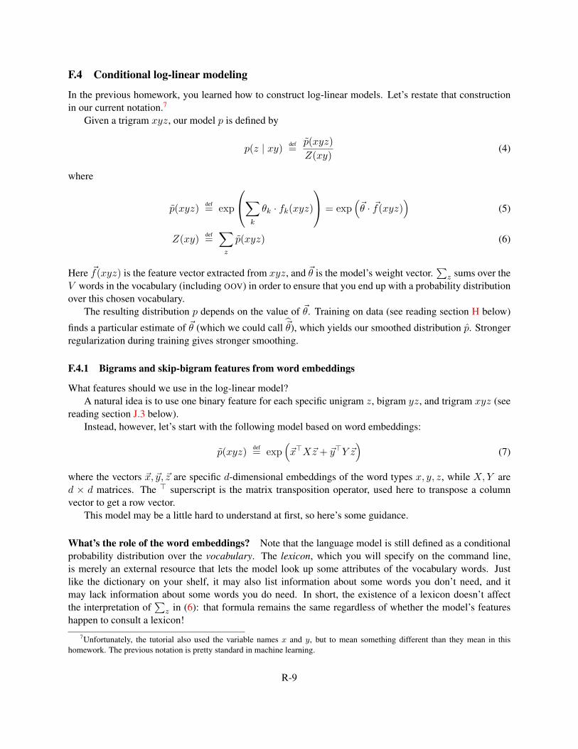
F.4 Conditional log-linear modeling

In the previous homework, you learned how to construct log-linear models. Let’s restate that constructionin our current notation.7

Given a trigram xyz, our model p is defined by

p(z | xy) def=

p(xyz)

Z(xy)(4)

where

p(xyz)def= exp

∑k

θk · fk(xyz)

= exp(~θ · ~f(xyz)

)(5)

Z(xy)def=∑z

p(xyz) (6)

Here ~f(xyz) is the feature vector extracted from xyz, and ~θ is the model’s weight vector.∑

z sums over theV words in the vocabulary (including OOV) in order to ensure that you end up with a probability distributionover this chosen vocabulary.

The resulting distribution p depends on the value of ~θ. Training on data (see reading section H below)

finds a particular estimate of ~θ (which we could call ~θ), which yields our smoothed distribution p. Strongerregularization during training gives stronger smoothing.

F.4.1 Bigrams and skip-bigram features from word embeddings

What features should we use in the log-linear model?A natural idea is to use one binary feature for each specific unigram z, bigram yz, and trigram xyz (see

reading section J.3 below).Instead, however, let’s start with the following model based on word embeddings:

p(xyz)def= exp

(~x>X~z + ~y>Y ~z

)(7)

where the vectors ~x, ~y, ~z are specific d-dimensional embeddings of the word types x, y, z, while X,Y ared × d matrices. The > superscript is the matrix transposition operator, used here to transpose a columnvector to get a row vector.

This model may be a little hard to understand at first, so here’s some guidance.

What’s the role of the word embeddings? Note that the language model is still defined as a conditionalprobability distribution over the vocabulary. The lexicon, which you will specify on the command line,is merely an external resource that lets the model look up some attributes of the vocabulary words. Justlike the dictionary on your shelf, it may also list information about some words you don’t need, and itmay lack information about some words you do need. In short, the existence of a lexicon doesn’t affectthe interpretation of

∑z in (6): that formula remains the same regardless of whether the model’s features

happen to consult a lexicon!7Unfortunately, the tutorial also used the variable names x and y, but to mean something different than they mean in this

homework. The previous notation is pretty standard in machine learning.

R-9

For OOV, or for any other type in your vocabulary that has no embedding listed in the lexicon, yourfeatures should back off to the embedding of OOL—a special “out of lexicon” symbol that stands for “allother words.” OOL is listed in the lexicon, just as OOV is included in the vocabulary.

Note that even if an specific out-of-vocabulary word is listed in the lexicon, you must not use that listing.8

For an out-of-vocabulary word, you are supposed to be computing probabilities like p(OOV | xy), whichis the probability of the whole OOV class—it doesn’t even mention the specific word that was replaced byOOV. (See reading section D.2.)

Is this really a log-linear model? Now, what’s up with (7)? It’s a valid formula: you can always geta probability distribution by defining p(z | xy) = 1

Z(xy) exp(any function of x, y, z that you like)! Butis (7) really a log-linear function? Yes it is! Let’s write out those d-dimensional vector-matrix-vectormultiplications more explicitly:

p(xyz) = exp

d∑j=1

d∑m=1

xjXjmzm +d∑j=1

d∑m=1

yjYjmzm

(8)

= exp

d∑j=1

d∑m=1

Xjm · (xjzm) +d∑j=1

d∑m=1

Yjm · (yjzm)

(9)

This does have the log-linear form of (5). Suppose d = 2. Then implicitly, we are using a weight vector ~θof length d2 + d2 = 8, defined by

〈 θ1, θ2, θ3, θ4, θ5, θ6, θ7, θ8 〉↓ ↓ ↓ ↓ ↓ ↓ ↓ ↓〈X11 , X12 , X21 , X22 , Y11 , Y12 , Y21 , Y22 〉

(10)

for a vector ~f(xyz) of 8 features

〈f1(xyz), f2(xyz), f3(xyz), f4(xyz), f5(xyz), f6(xyz), f7(xyz), f8(xyz) 〉↓ ↓ ↓ ↓ ↓ ↓ ↓ ↓

〈 x1z1, x1z2, x2z1, x2z2, y1z1, y1z2, y2z1, y2z2 〉(11)

Remember that the optimizer’s job is to automatically manipulate some control sliders. This particularmodel with d = 2 has a control panel with 8 sliders, arranged in two d×d grids (X and Y ). The point is thatwe can also refer to those same 8 sliders as θ1, . . . θ8 if we like. What features are these sliders (weights) beconnected to? The ones in (11): if we adopt those feature definitions, then our general log-linear formula(5) will yield up our specific model (9) (= (7)) as a special case.

What keeps (7) log-linear is that the feature functions are pre-specified functions of xyz as shown inequation (11). Specifically, they are determined by the word embeddings ~x, ~y, and ~z. We are not going tolearn the word embeddings or the feature functions fk—we only have to learn the weights θk.

As always, the learned weight vector ~θ is incredibly important: it determines all the probabilities in themodel.

8This issue would not arise if we simply defined the vocabulary to be the set of words that appear in the lexicon. This simplestrategy is certainly sensible, but it would slow down normalization because our lexicon is quite large.

R-10

Is this a sensible model? The feature definitions in (11) are pairwise products of embedding dimensions.Why on earth would such features be useful? First imagine that the embedding dimensions were bits (0or 1). Then x2z1 = 1 iff (x2 = 1 and z1 = 1), so you could think of multiplication as a kind of featureconjunction. Multiplication has a similar conjunctive effect even when the embedding dimensions are in R.For example, suppose z1 > 0 indicates the degree to which z is a human-like noun, while x2 > 0 indicatesthe degree to which x is a verb whose direct objects are usually human.9 Then the product x2z1 will be largerfor trigrams like kiss the baby and marry the policeman. So by learning a positive weightX21

(nicknamed θ3 above), the optimizer can drive p(baby | kiss the) higher, at the expense of probabilitieslike p(benzene | kiss the). p(bunny | kiss the) might be somewhere in the middle since bunniesare a bit human-like and thus bunny1 might be numerically somewhere between baby1 and benzene1.

Example. As an example, let’s calculate the letter trigram probability p(s | er). Suppose the relevantletter embeddings and the feature weights are given by

~e =

[−.51

], ~r =

[0.5

], ~s =

[.5.5

], X =

[1 00 .5

], Y =

[2 00 1

]First, we compute the unnormalized probability.

p(ers) = exp

[−.5 1]

[1 00 .5

][.5.5

]+ [0 .5]

[2 00 1

][.5.5

]= exp(−.5× 1× .5 + 1× .5× .5 + 0× 2× .5 + .5× 1× .5) = exp 0.25 = 1.284

We then normalize p(ers).

p(s | er) def=

p(ers)

Z(er)=

p(ers)

p(era) + p(erb) + · · ·+ p(erz)=

1.284

1.284 + · · ·(12)

Speedup. The example illustrates that the denominator

Z(xy) =∑z′

p(xyz′) =∑z′

exp(~x>X~z′ + ~y>Y ~z′

)(13)

is expensive to compute because of the summation over all z′ in the vocabulary. Fortunately, you can com-pute x>Xz′ ∈ R simultaneously for all z′.10 The results can be found as the elements of the row vectorx>XE, where E is a d × V matrix whose columns are the embeddings of the various words z′ in the vo-cabulary. This is easy to see, and computing this vector still requires just as many scalar multiplications andadditions as before . . . but we have now expressed the computation as a pair of vector-matrix mutiplications,(x>X)E, which you can perform using library calls in PyTorch (similarly to another matrix library, numpy).That can be considerably faster than looping over all z′. That is because the library call is highly optimizedand exploits hardware support for matrix operations (e.g., parallelism).

9You might wonder: What if the embedding dimensions don’t have such nice interpretations? What if z1 doesn’t represent asingle property like humanness, but rather a linear combination of such properties? That actually doesn’t make much difference.Suppose z can be regarded asMz where z is a more interpretable vector of properties. (Equivalently: each zj is a linear combinationof the properties in z.) Then x>Xz can be expressed as (Mx)>X(My) = x>(M>XM)y. So now it’s X = M>XM that canbe regarded as the matrix of weights on the interpretable products. If there exists a good X and M is invertible, then there exists agood X as well, namely X = (M>)−1XM−1.

10The same trick works for y>Y z′, of course.

R-11

F.5 Other smoothing schemes

Numerous other smoothing schemes exist. In past years, for example, our course homeworks have usedWitten-Bell backoff smoothing, or Katz backoff with Good–Turing discounting.

In practical settings, the most popular n-gram smoothing scheme is something called modified Kneser–Ney. One can also use a more principled Bayesian method based on the hierarchical Pitman–Yor process;the resulting formulas are very close to modified Kneser–Ney.

Remember: While these techniques are effective, a really good language model would do more than justsmooth n-gram probabilities well. To predict a word sequence as accurately as a human can finish anotherhuman’s sentence, it would go beyond the whole n-gram family to consider syntax, semantics, and topicthroughout a sentence or document. It would also use common sense and factual knowledge about the world.Thus, language modeling remains an active area of research that uses grammars, recurrent neural networks,and other techniques.

Indeed, it is reasonable to say that language modeling is AI-complete. That is, we can’t solve languagemodeling without solving pretty much all of AI. This was essentially the point of Alan Turing’s 1950 article“Computing Machinery and Intelligence,” in which he considered the possibility of a machine that couldsustain a deep, wide-ranging conversation. His “Turing Test” involves making you guess whether you’reconversing with a computer or a human. If you can’t tell, then maybe you should accept that the computeris intelligent in some sense.11

(It follows that progress in language modeling might inadvertently create progress in AI. The enormousGPT-3 model (reading section A) is already startlingly good at generating sentences that are appropriatein context. It has no explicit representation of grammar, knowledge, or reasoning—yet by learning how tomodel its training corpus, it has implicitly picked up a lot of whatever is needed to generate intelligent text.While it is still imperfect in many ways, its creators demonstrated that we can interrogate it to get answersto other AI problems that it was not specifically designed to solve.)

G Safe practices for working with log-probabilities

G.1 Use natural log for internal computations

In this homework, as in most of mathematics, log means loge (the log to base e, or natural log, sometimeswritten ln). This is also the standard behavior of the log function in most programming languages.

With natural log, the calculus comes out nicely, thanks to the fact that ddZ logZ = 1

Z . It’s only withnatural log that the gradient of the log-likelihood of a log-linear model can be directly expressed as observedfeatures minus expected features.

On the other hand, information theory conventionally talks about bits, and quantities like entropy andcross-entropy are conventionally measured in bits. Bits are the unit of − log2 probability. A probability of0.25 is reported “in negative-log space” as − log2 0.25 = 2 bits. Some people do report that value moresimply as− loge 0.25 = 1.386 nats. But it is more conventional to use bits as the unit of measurement. (Theterm “bits” was coined in 1948 by Claude Shannon to refer to “binary digits,” and “nats” was later definedby analogy to refer to the use of natural log instead of log base 2. The unit conversion factor is 1

log 2 ≈ 1.443bits/nat.)

11Perhaps the computer still can’t perceive and manipulate physical objects, so there are parts of AI (robotics and vision) thatit isn’t solving. But it still has to be able to talk about the physical world, and Turing’s proposal was that that being able to talksensibly about things should be enough to qualify as intelligent.

R-12

Even if you are planning to print bit values, it’s still wise to standardize on loge-probabilities for allof your formulas, variables, and internal computations. Why? They’re just easier! If you tried to usenegative log2-probabilities throughout your computation, then whenever you called the log function ortook a derivative, you’d have to remember to convert the result. It’s too easy to make a mistake by omittingthis step or by getting it wrong. So the best practice is to do this unit conversion only when you print: at thatpoint convert your loge-probability from negative nats to positive bits by dividing by − log 2 ≈ −0.693.

G.2 Avoid exponentiating big numbers (crucial for gen/spam!)

Log-linear models require calling the exp function. Unfortunately, exp(710) is already too large for a 64-bitfloating-point number to represent, and will generate a runtime error (“overflow”). Conversely, exp(−746)is too close to 0 to represent, and will simply return 0 (“underflow”).

That shouldn’t be a problem for this homework if you stick to the language ID task. If you are experi-encing an overflow issue there, then your parameters probably became too positive or too negative as youran stochastic gradient descent, or because of the way you randomly initialized your model’s parameters.

But to avoid these problems elsewhere—including with the spam detection task—the standard trick isto represent all values “in log-space.” In other words, simply store 710 and −746 rather than attempting toexponentiate them.

But how can you do arithmetic in log-space? Suppose you have two numbers p, q, which you arerepresenting in memory by their logs, lp and lq.

• Multiplication: You can represent pq by its log, log(pq) = log(p) + log(q) = lp + lq. That is,multiplication corresponds to log-space addition.

• Division: You can represent p/q by its log, log(p/q) = log(p) − log(q) = lp − lq. That is, divisioncorresponds to log-space subtraction.

• Addition: You can represent p+q by its log. log(p+q) = log(exp(lp)+exp(lq)) = logaddexp(lp, lq).See the discussion of logaddexp and logsumexp in the future Homework 6 handout. These areavailable in PyTorch.

For training a log-linear model, you can work almost entirely in log space, representing u and Z inmemory by their logs, log u and logZ. In order to compute the expected feature vector in (18) below,you will need to come out of log space and find p(z′ | xy) = u′/Z for each word z′. But computingu′ and Z separately is dangerous: they might be too large or too small. Instead, rewrite p(z′ | xy) asexp(log u′ − logZ). Since u′ ≤ Z, this is exp of a negative number, so it will never overflow. It mightunderflow to 0 for some words z′, but that’s ok: it just means that p(z′ | xy) really is extremely close to 0,and so ~f(xyz′) should make only a negligible contribution to the expected feature vector.

R-13

H Training a log-linear model

H.1 The training objective

To implement the conditional log-linear model, the main work is to train ~θ (given some training data and aregularization coefficient C). As usual, you’ll set ~θ to maximize

F (~θ)def=

1

N

N∑i=1

log p(wi | wi−2 wi−1)

︸ ︷︷ ︸

log likelihood

−

C ·∑k

θ2k

︸ ︷︷ ︸

L2 regularizer

(14)

which is the L2-regularized log-likelihood per word token. (There are N word tokens.)So we want ~θ to make our training corpus probable, or equivalently, to make the N events in the corpus

(including the final EOS) probable on average given their bigram contexts. At the same time, we also wantthe weights in ~θ to be close to 0, other things equal (regularization).12

The regularization coefficient C ≥ 0 can be selected based on dev data.

H.2 Stochastic gradient descent

Fortunately, concave functions like F (~θ) in (14) are “easy” to maximize. You can implement a simplestochastic gradient descent (SGD) method to do this optimization.

More properly, this should be called stochastic gradient ascent, since we are maximizing rather thanminimizing, but that’s just a simple change of sign. The pseudocode is given by Algorithm 1. We rewritethe objective F (~θ) given in (14) as an average of local objectives Fi(~θ) that each predict a single word, bymoving the regularization term into the summation.

F (~θ) =1

N

N∑i=1

log p(wi | wi−2 wi−1)−C

N·∑k

θ2k

︸ ︷︷ ︸

call this Fi(~θ)

(16)

=1

N

N∑i=1

Fi(~θ) (17)

The gradient of this average,∇F (~θ), is therefore the average value of∇Fi(~θ).12As explained on the previous homework, this can also be interpreted as maximizing p(~θ | ~w)—that is, choosing the most

probable ~θ given the training corpus. By Bayes’ Theorem, p(~θ | ~w) is proportional to

p(~w | ~θ)︸ ︷︷ ︸likelihood

· p(~θ)︸︷︷︸prior

(15)

Let’s assume an independent Gaussian prior over each θk, with variance σ2. Then if we take C = 1/2σ2, maximizing (14) is justmaximizing the log of (15). The reason we maximize the log is to avoid underflow, and because the derivatives of the log happento have a simple “observed− expected” form (since the log sort of cancels out the exp in the definition of p(xyz).)

R-14

Algorithm 1 Stochastic gradient ascent

Input: Initial stepsize γ0, initial parameter values ~θ(0), training corpus D = (w1, w2, · · · , wN ), regulariza-tion coefficient C, number of epochs E

1: procedure TRAIN

2: ~θ ← ~θ(0)

3: t← 0 . number of updates so far4: for e : 1→ E : . do E passes over the training data, or “epochs”5: for i : 1→ N : . loop over summands of (16)6: γ ← γ0

1 + γ0 · 2CN · t. current stepsize—decreases gradually

7: ~θ ← ~θ + γ · ∇Fi(~θ) . move ~θ slightly in a direction that increases Fi(~θ)8: t← t+ 1

9: return ~θ

Discussion. On each iteration, the algorithm picks some word i and pushes ~θ in the direction ∇Fi(~θ),which is the direction that gets the fastest increase in Fi(~θ). The updates from different i will partly cancelone another out,13 but their average direction is∇F (~θ), so their average effect will be to improve the overallobjective F (~θ). Since we are training a log-linear model, our F (~θ) is a concave function with a single globalmaximum; a theorem guarantees that the algorithm will converge to that maximum if allowed to run forever(E =∞).

How far the algorithm pushes ~θ is controlled by γ, known as the “step size” or “learning rate.” Thisstarts at γ0, but needs to decrease over time in order to guarantee convergence of the algorithm. The rule inline 6 for gradually decreasing γ works well with our specific L2-regularized objective (14).14

Note that t increases and the stepsize decreases on every pass through the inner loop. This is importantbecause N might be extremely large in general. Suppose you are training on the whole web—then thestochastic gradient ascent algorithm should have essentially converged even before you finish the first epoch!See reading section I.8 for some more thoughts about epochs.

H.3 The gradient vector

The gradient vector ∇Fi(~θ) is merely the vector of partial derivatives(∂Fi(~θ)∂θ1

, ∂Fi(~θ)∂θ2

, . . .

). where Fi(~θ)

was defined in (16). As you’ll recall from the previous homework, each partial derivative takes a simple and

13For example, in the training sentence eat your dinner but first eat your words, ∇F3(~θ) is trying to raisethe probability of dinner, while ∇F8(~θ) is trying to raise the probability of words (at the expense of dinner!) in the samecontext.

14It is based on the discussion in section 5.2 of Bottou (2012), “Stochastic gradient descent tricks,” who has this objective asequation (10). You should read that paper in full if you want to use SGD “for real” on your own problems.

R-15

beautiful form15

∂Fi(~θ)

∂θk= fk(xyz)︸ ︷︷ ︸

observed value of feature fk

−∑z′

p(z′ | xy)fk(xyz′)︸ ︷︷ ︸expected value of feature fk , according to current p

− 2C

Nθk︸ ︷︷ ︸

pulls θk towards 0

(18)

where x, y, z respectively denote wi−2, wi−1, wi, and the summation variable z′ in the second term rangesover all V words in the vocabulary, including OOV. This obtains the partial derivative by summing multiplesof three values: the observed feature count in the training data, the expected feature counts ccording to thecurrent p (which is based on the entire current ~θ, not just θk), and the current weight θk itself.

H.4 The gradient for the embedding-based model

When we use the specific model in (7), the feature weights are the entries of theX and Y matrices, as shownin (9). The partial derivatives with respect to these weights are

∂Fi(~θ)

∂Xjm= xjzm −

∑z′

p(z′ | xy)xjz′m −2C

NXjm (19)

∂Fi(~θ)

∂Yjm= yjzm −

∑z′

p(z′ | xy)yjz′m −2C

NYjm (20)

where as before, we use ~x, ~y, ~z, ~z ′ to denote the embeddings of the words x, y, z, z′. Thus, the update to ~θ(Algorithm 1, line 7) is

(∀j,m = 1, 2, . . . d) Xjm ← Xjm + γ · ∂Fi(~θ)

∂Xjm(21)

(∀j,m = 1, 2, . . . d) Yjm ← Yjm + γ · ∂Fi(~θ)

∂Yjm(22)

I Practical hints for stochastic gradient ascent

The magenta hyperlinks in this section may be particularly useful. Most of them link to PyTorch documen-tation.

I.1 Use automatic differentiation

You don’t actually have to implement the gradient computations in reading sections H.3 to H.4! You could,of course. But the backward method in PyTorch will automatically compute the vector of partial deriva-tives for you, using a technique known as automatic differentiation by back-propagation (or simply “back-

15This formula shows the partial derivative with respect to θk only. If you prefer to think of computing the whole gradient vector,for all k at once, you can equivalently write this using vector computations as

∇Fi(~θ) = ~f(xyz)−∑z′

p(z′ | xy)~f(xyz′)− 2C

N~θ

.

R-16

prop”). So, you only have to implement the “forward” computation Fi(~θ) for a given example i, and Py-Torch will be able to “work backward” and find∇Fi(~θ). This requires it to determine how small changes to~θ would have affected Fi(~θ). See reading section I.6 below for details.

If the forward computation is efficient and correct, then the backward computation as performed bybackward will also be efficient and correct. If instead you wrote your own code to compute the gradient,it would be easy to mess up and miss an algebraic optimization—you could end up takingO(V 2) time whenO(V ) is possible. You’d also have to put in checks to make sure that you were actually computing thegradient correctly (e.g., the “finite-difference check”). This is not necessary nowadays.

I.2 Don’t try to learn all of PyTorch

We won’t be learning the whole PyTorch framework in this class, although it’s very nicely designed. All weneed is the basics:

• rapidly manipulate tensors (multidimensional numeric arrays), just as in NumPy, Matlab, and otherscientific computing packages

• automatically compute gradients via backward

(If you’ve built neural nets in PyTorch before, for example in the Deep Learning class, then you mayhave written models by extending torch.nn.Module and instantiating the forwardmethod. However,we’re going to avoid using torch.nn. If you’re used to relying on it, check out Neural net from scratchto see how to train a network with the PyTorch basics only. That link is the starting point for an explanationof how torch.nn can optionally be used to streamline the code, but you don’t need that.)

I.3 Make the forward computation efficient

In general, use PyTorch’s tensor operations wherever possible. One such operation can do a lot of computa-tion, and is much faster than doing the same work with a Python loop. Avoid Python loops!

When the vocabulary is large, the slowest part of the forward computation Fi(~θ) is computing the de-nominatorZ(xy) for each xy that you find, because it involves computing p(xyz) for all z and then summingover all of them. You can use fast PyTorch operations for this.16

(Advanced remark: There are language models that eliminate the need to sum over the whole vocabularyby predicting each word one bit at a time (Mnih and Hinton (2009)). Then you only have to predict asequence of log2 V bits. Since each prediction is only over two options, the denominator in the probabilityonly has to sum over 2 choices instead of V choices. This is computationally faster, but predicting thosebits is a somewhat artificial task that’s hard to do accurately. Nowadays people seem to just do the V -wayprediction, ideally using a GPU to accelerate the PyTorch operations.)

I.4 Make the forward computation correct

Our probability model p(z | xy) predicts the next word z from the vocabulary. Thus, the denominator Z inequation (6) should sum over the vocabulary of possible next words (including EOS and OOV). It should notsum over the lexicon, which is quite different! There might be dozens of vocabulary words that are not in

16In principle, it could be helpful to “memoize” Z(xy) in a dictionary, so that if you see the same xy many times, you don’t haveto recompute Z(xy) again each time: you can just look it up. Unfortunately, you do still have to recompute Z(xy) if ~θ has changedsince the last time you computed it. Since ~θ changes often with SGD, this trick may not give a net win.

R-17

the lexicon: but we still have to add them into Z, using the OOL embedding for each of them. Conversely,there might be thousands of lexicon words that are not in the vocabulary: the model simply can’t generateany of them, although it can generate OOV.

To enable fast computation of Z, you can precompute a matrix of embeddings of the vocabulary wordsusing torch.stack:

torch.stack([embedding(word) for word in self.vocab])

where embedding(word) looks up the embedding of a word in the lexicon (returning the OOL embeddingif necessary). For this to be correct, self.vocab includes EOS and OOV.

For reasons discussed in reading section G.2, you won’t want to compute p(z | xy) directly using equa-tion (4). Instead, you’ll want to compute log p(z | xy) = log p(xyz) − logZ(xy), where you’d better uselogsumexp to help find logZ(xy). For example, torch.logsumexp(torch.Tensor([1,2,3]),0)or equivalently torch.Tensor([1,2,3]).logsumexp(0) is mathematically equivalent tolog(exp(1)+exp(2)+exp(3)), but is faster and more numerically stable.17

What is the reason for the 0 argument in these expressions? It specifies which dimension of the tensor tooperate on. In the example above, we are applying logsumexp to a 1D tensor (vector), so the only possibledimension is 0. But if A is a 2D tensor (matrix), then A.logsumexp(0) sums up each row separately,whereas A.logsumexp(1) sums up each column separately. This may actually be useful later in theassignment: if you try the mini-batching technique in reading section I.8.4 below, you might be computinglogZ(xy) for many different contexts at once.

I.5 Choose your hyperparameters carefully

The convergence speed of stochastic gradient ascent is sensitive to the initial learning rate γ0. We recom-mend trying γ0 = 0.1 for spam detection or γ0 = 0.01 for language ID.

The initial guess ~θ(0) also matters. The easiest choice is ~0 (i.e., initialize all entries of X and Y to 0),and that will work fine in this case, although it is not recommended in general.18

(Note that the homework asks you to use the hyperparameters recommended above when log linearis selected (question 7(b)). This will let you and us check that your implementation is correct. However,you may want to experiment with different settings, and you are free to use those other settings whenlog linear improved is selected, to get better performance.)

I.6 Compute and apply the gradient properly

To implement line 7 of Algorithm 1, you should do something like this:17When you’re adding up thousands of terms using log(exp(1)+exp(2)+exp(3)+· · ·), the resulting logZ may be nu-

merically imprecise—and its gradient will be so imprecise that trying to follow it actually won’t be able to find good parametersfor the model!

18To see what could go wrong, imagine that we were not given the word embeddings in a file, but were learning them along withX and Y . Such a model would be symmetric—different dimensions of the embeddings would be governed by the same equations.As a result, if we initialized all parameters to 0, then all parameters of the same kind would have to have identical updates, andtherefore, they would continue to have identical values throughout optimization!

The standard solution is to initialize the parameters not to 0, but to random values close to 0—for example, drawn from a normaldistribution with mean 0 and small standard deviation. This “breaks the symmetry” and allows the different dimensions of the wordembeddings to specialize and play different roles.

The performance of the model is then sensitive to the random initialization. A common technique is “random restarts”: trainseveral times, initializing randomly each time, and return the trained parameters that worked best on development data.

R-18

F_i = log_prob - regularizer # as defined in (16); depends on ~θ and on example i

F_i.backward() # increases ~θ.grad by the vector (∂Fi

∂θ1, ∂Fi

∂θ2, . . .)

The first line is the final step of the forward computation, and the second line is the backward computation.The parameters don’t actually have to be named ~θ. For example, the probability model given by equa-

tions (4) to (7) has parameter matrices X and Y . Suppose we represent those as 2D tensors X and Y, andthen use them to help compute F_i. Then X.grad and Y.grad will be magically defined to be 2D ten-sors of the same shapes as X and Y. The call to F_i.backward() serves to modify both of them: forexample, it will increase (X.grad)[5,2] by ∂Fi

∂X[5,2] . To make this happen, however, you need to specifybefore doing the forward computation that X and Y should track their gradients: either create them with therequires grad=True flag, or call their requires grad (true)method right after you create them.

After doing the backward computation, to complete line 7, you can update X and Y like this:

with torch.no_grad():F += F_i # keep a running total of F over the epoch, if you likeX += gamma * X.grad # update X in the direction that will increase FiY += gamma * Y.grad # update Y in the direction that will increase Fi

The no grad directive says not to track the computations in this block of code, because we don’t need thegradient of those computations. It would be very expensive if F , X , and Y had to remember all the stepsthat computed them! After all, F depends on all of the trigrams in this epoch, and the current values of Xand Y depend on all of the updates from all of the epochs so far. If you kept track of all these computationsat once, you would probably run out of memory during training. Fortunately, we only need to keep trackof the computations for the current F_i, not the total F. Once we call F_i.backward(), and take thestochastic gradient step, we are allowed to forget how F_i was computed. This happens automaticallybecause on the next iteration of the loop, F_i is assigned to a new value. The old value and its attachedcomputation are then no longer accessible (as long as we’re not tracking the computation of F), so Pythoncan garbage-collect them when it gets low on memory.

Finally, remember that the backward algorithm doesn’t set the grad tensors; it increases them, addingto whatever is already there. This is because of how the backprop algorithm works internally: it accumu-lates an answer into grad by successive addition. Thus, you must explicitly clean up by resetting theseaccumulators to 0 before the next call to backward.

X.grad.zero_()Y.grad.zero_()

The method name zero_ ends in _ because it modifies the tensor in place; this is a PyTorch convention.

I.7 Manage parameter updates using a PyTorch optimizer

One annoying thing about the approach of reading section I.6 is that you have to explicitly update both Xand Y, and you have to explictly reset both X.grad and Y.grad. The more complex your model, the morevariables there are to worry about. The torch.nn module can help with this, if you like:

• keep track of all of the model parameters via torch.nn.Parameter• update those parameters via SGD or another optimizer of your choice

This is illustrated in the starter code we provided you. EmbeddingLogLinearLanguageModel inher-its from torch.nn.Module for this reason. When an instance of this model is created, it registers thetensors X and Y as parameters of the model. Now all of the code in reading section I.6 can be simplified to

R-19

F_i = log_prob - regularizer # as before(-F_i).backward() # note change of signoptimizer.step() # adjusts the parameters (X and Y)optimizer.zero_grad() # resets the gradient tensors (X.grad and Y.grad)

The optimizer object manages the state of an optimization algorithm such as SGD. The starter codeshows how to create a basic SGD optimizer via torch.optim.SGD. By convention, PyTorch optimizersminimize an objective function by taking a step in the direction that will decrease the function. That is,optimizer insists on doing stochastic gradient descent rather than ascent. So instead of maximizingF =

∑i Fi, we will use it to minimize −F =

∑i(−Fi). That is why we find the gradient of -F_i above.

I.8 Improve the SGD training loop

The following improvements are not required for the homework, but they might help you run faster or getbetter results. You should read this section in any case.

I.8.1 Convergent SGD

torch.optim.SGD won’t decrease the learning rate on every step. But decreasing the stepsize in anappropriate way (as in Algorithm 1) is necessary to guarantee that the SGD optimizer eventually convergesto a local minimum.

In the special case of log-linear models, our objective function (the negative of equation (14)) happensto be convex, so it has a unique local minimum—namely the global minimum. You might as well useAlgorithm 1 to be sure that that you converge to that. Any initial stepsize γ0 > 0 and decrease rate λ > 0will suffice (the choice λ = 2C

N is the one we used in reading section H.2).(Why doesn’t torch.optim.SGD already decrease the learning rate? Because it is mostly used for

deep learning where the objective function is not convex and has lots of local minima. Some of the localminima overfit to the training data despite regularization. There is some evidence that keeping a constantlearning rate will actually do better at avoiding these bad local minima.)

I.8.2 Deciding when to stop

In reading section H.2, you may have wondered how to choose E, the number of epochs. We are usinga fixed number of epochs only to keep things simple. The more traditional SGD approach is to continuerunning until the function appears to have converged “well enough.” For example, you could stop if theaverage gradient over the past epoch (or the past m examples) was very small.

In machine learning, our ultimate goal is not actually to optimize the training objective, but rather to dowell on test data. Thus, a more common approach in machine learning is to compute the evaluation metric(reading section E) on development data at the end of each epoch (or after each group of m examples).Stop if that “dev objective” has failed to improve (say) 3 times in a row. Then you can use the parametervector ~θ that performed best on development data. This is known as “early stopping” because SGD may notyet have converged to an optimum on the training objective. Early stopping can be an effective regularizer(especially when C is too small) since it prevents overfitting to the training data. In effect, early stoppingtreats the number of epochs as a hyperparameter that is tuned on dev data. It’s efficient and effective.

R-20

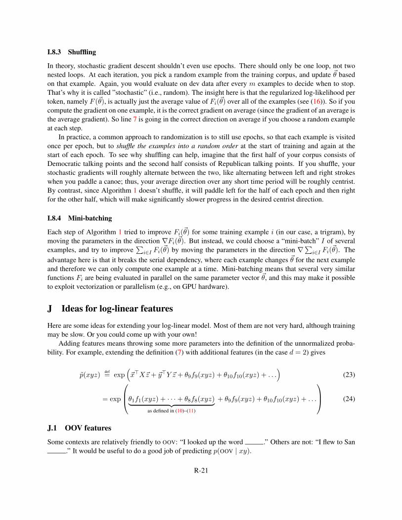
I.8.3 Shuffling

In theory, stochastic gradient descent shouldn’t even use epochs. There should only be one loop, not twonested loops. At each iteration, you pick a random example from the training corpus, and update ~θ basedon that example. Again, you would evaluate on dev data after every m examples to decide when to stop.That’s why it is called ”stochastic” (i.e., random). The insight here is that the regularized log-likelihood pertoken, namely F (~θ), is actually just the average value of Fi(~θ) over all of the examples (see (16)). So if youcompute the gradient on one example, it is the correct gradient on average (since the gradient of an average isthe average gradient). So line 7 is going in the correct direction on average if you choose a random exampleat each step.

In practice, a common approach to randomization is to still use epochs, so that each example is visitedonce per epoch, but to shuffle the examples into a random order at the start of training and again at thestart of each epoch. To see why shuffling can help, imagine that the first half of your corpus consists ofDemocratic talking points and the second half consists of Republican talking points. If you shuffle, yourstochastic gradients will roughly alternate between the two, like alternating between left and right strokeswhen you paddle a canoe; thus, your average direction over any short time period will be roughly centrist.By contrast, since Algorithm 1 doesn’t shuffle, it will paddle left for the half of each epoch and then rightfor the other half, which will make significantly slower progress in the desired centrist direction.

I.8.4 Mini-batching

Each step of Algorithm 1 tried to improve Fi(~θ) for some training example i (in our case, a trigram), bymoving the parameters in the direction ∇Fi(~θ). But instead, we could choose a “mini-batch” I of severalexamples, and try to improve

∑i∈I Fi(

~θ) by moving the parameters in the direction ∇∑

i∈I Fi(~θ). The

advantage here is that it breaks the serial dependency, where each example changes ~θ for the next exampleand therefore we can only compute one example at a time. Mini-batching means that several very similarfunctions Fi are being evaluated in parallel on the same parameter vector ~θ, and this may make it possibleto exploit vectorization or parallelism (e.g., on GPU hardware).

J Ideas for log-linear features

Here are some ideas for extending your log-linear model. Most of them are not very hard, although trainingmay be slow. Or you could come up with your own!

Adding features means throwing some more parameters into the definition of the unnormalized proba-bility. For example, extending the definition (7) with additional features (in the case d = 2) gives

p(xyz)def= exp

(~x>X~z + ~y>Y ~z + θ9f9(xyz) + θ10f10(xyz) + . . .

)(23)

= exp

θ1f1(xyz) + · · ·+ θ8f8(xyz)︸ ︷︷ ︸as defined in (10)–(11)

+ θ9f9(xyz) + θ10f10(xyz) + . . .

(24)

J.1 OOV features

Some contexts are relatively friendly to OOV: “I looked up the word .” Others are not: “I flew to San.” It would be useful to do a good job of predicting p(OOV | xy).

R-21

Unfortunately, our basic model (7) does not have the freedom to learn specific parameters for OOV. Itjust uses its general parameters X,Y with the pre-specified embedding of OOV.

Worse yet, the embedding of OOV is inappropriate. Recall from reading section F.4.1 that when z =OOV, equation (7) takes ~z to be the embedding of OOL, since OOV is not in the lexicon. But that means OOV

is treated just like any other out-of-lexicon word. That’s wrong—typically, OOV should have a much higherprobability than any specific out-of-lexicon word that is in the vocabulary, because it represents a wholeclass of words: p(OOV | xy) stands for the total probability of all words that are out-of-vocabulary.

Thus, you might add a simple feature foov(xyz) that returns 1 if z = OOV and returns 0 otherwise.Given any xy, the expression ~xX~z + ~yY ~z is still equal for all OOL elements of the vocabulary, since theyall have the same ~z. But when z = OOV, the extra feature foov now fires as well, which increases p(xyz)by a factor of exp θoov. As a result, for any xy, p(xyz) is exactly exp θoov times larger when z = OOV thanwhen z is some specific OOL word. The trained value of θoov determines how big this factor is. Roughlyspeaking, this factor should be large if the original training corpus had a lot of different OOV word types.

You could be fancier and try to learn different OOV parameters for the different dimensions. For example,you could add this to the score of xyz before you exponentiate:{

~x · ~xoov + ~y · ~yoov if z = OOV

0 otherwise(25)

Here ~xoov and ~yoov are learned parameter vectors, so in effect we are learning 2d additional feature weights.This should do a better job of learning how much to raise (or lower) the probability of z = OOV accordingto the various properties of the context words x and y. Convince yourself that this model is still log-linear.19

J.2 Unigram log-probability

More generally, a weakness of the model (7) is that it doesn’t have any parameters that keep track of howfrequent specific words are in the training corpus! Rather, it backs off from the words to their embeddings.Its probability estimates are based only on the embeddings, which were learned from some other (larger)corpus.

It’s pretty common in NLP to use SGD to adjust the embeddings at the same time as the other parameters.But then we wouldn’t have a log-linear model anymore, as discussed below equation (11).

One way to fix the weakness while staying within the log-linear framework would be to have a binaryfeature fw for each word w in the vocabulary, such that fw(xyz) is 1 if z = w and 0 otherwise. We’ll dothat in section J.3 below.

But first, here’s a simpler method: just add a single non-binary feature defined by

funigram(xyz) = log punigram(z) (26)

where punigram(z) is estimated by add-1 smoothing. Surely we have enough training data to learn an appro-priate weight for this single feature. In fact, because every training token wi provides evidence about thissingle feature, its weight will tend to converge quickly to a reasonable value during SGD.

This is not the only feature in the model—as usual, you will use SGD to train the weights of all featuresto work together, computing the gradient via (18). Let β = θunigram denote the weight that we learn for

19An alternative would be to replace OOV’s embedding ~z with a new, learned embedding vector ~zoov. Is that still log-linear? Well,if we only use the new embedding in the z position, then we’re changing the score of xyz from ~x>X~z + ~y>Y ~z to ~x>X~zoov +~y>Y ~zoov. But we can get exactly the same effect with the scheme above by learning ~xoov = X(~zoov − ~z) and ~yoov = Y (~zoov − ~z).

R-22

the new feature. By including this feature in our definition of punigram(z), we are basically multiplying afactor of (punigram(z))

β into the numerator p(xyz) (check (5) to see that this is true). This means that in thespecial case where β = 1 and X = Y = 0, we simply have p(xyz) = punigram, so that the log-linear modelgives exactly the same probabilities as the add-1 smoothed unigram model punigram. However, by trainingthe parameters, we might learn to trust the unigram model less (0 < β < 1) and rely more on the wordembeddings (X,Y 6= 0) to judge which words z are likely in the context xy.

A quick way to implement this scheme is to define

funigram(xyz) = log(c(z) + 1) (where c(z) is the count of z in training data) (27)

This gives the same model, since punigram(z) is just c(z)+ 1 divided by a constant, and our model renormal-izes p(xyz) by a constant anyway.

J.3 Unigram, bigram, and trigram indicator features

Try adding a unigram feature fw for each word w in the vocabulary. That is, fw(xyz) is 1 if z = w and 0otherwise. Does this work better than the log-unigram-probability feature from section J.2?

Now try also adding a binary feature for each bigram and trigram that appears at least 3 times in trainingdata. How good is the resulting model?

In all cases, you will want to tune C on development data to prevent overfitting. This is important—theoriginal model had only 2d2 + 1 parameters where d is the dimensionality of the embeddings, but your newmodel has enough parameters that it can easily overfit the training data. In fact, if C = 0, the new modelwill exactly predict the unsmoothed probabilities, as if you were not smoothing at all (add-0)! The reasonis that the maximum of the concave function F (~θ) =

∑Ni=1 Fi(

~θ) is achieved when its partial derivativesare 0. So for each unigram feature fw defined in the previous paragraph, we have, from equation (18) withC = 0,

∂F (~θ)

∂θw=

N∑i=1

∂Fi(~θ)

∂θw(28)

=N∑i=1

fw(xyz)︸ ︷︷ ︸observed count of w in corpus

−N∑i=1

∑z′

p(z′ | xy)fw(xyz′)︸ ︷︷ ︸predicted count of w in corpus

(29)

Hence SGD will adjust ~θ until this is 0, that is, until the predicted count of w exactly matches the observedcount c(w). For example, if c(w) = 0, then SGD will try to allocate 0 probability to word w in all contexts(no smoothing), by driving θw → −∞. Taking C > 0 prevents this by encouraging θw to stay close to 0.

J.4 Embedding-based features on unigrams and trigrams

Oddly, (7) only includes features that evaluate the bigram yz (via weights in the Y matrix) and the skip-bigram xz (via weights in the X matrix). After all, you can see in (9) that the features have the form yjzmand xjzm. This seems weaker than add-λ with backoff. Thus, add unigram features of the form zm andtrigram features of the form xhyjzm.

R-23

J.5 Embedding-based features based on more distant skip-bigrams

For a log-linear model, there’s no reason to limit yourself to trigram context. Why not look at 10 previouswords rather than 2 previous words? In other words, your language model can use the estimate p(wi |wi−10, wi−9, . . . wi−1).

There are various ways to accomplish this. You may want to reuse the X matrix at all positions i −10, i − 9, . . . , i − 2 (while still using a separate Y matrix at position i − 1). This means that having theword “bread” anywhere in the recent history (except at position wi−1) will have the same effect on wi. Sucha design is called “tying” the feature weights: if you think of different positions having different featuresassociated with them, you are insisting that certain related features have weights that are “tied together”(i.e., they share a weight).

You could further improve the design by saying that “bread” has weaker influence when it is in the moredistant past. This could be done by redefining the features: for example, in your version of (9), you couldscale down the feature value (xjzm) by the number of word tokens that fall between x and z.20

Note: The provided code has separate methods for 3-grams, 2-grams, and 1-grams. To support generaln-grams, you’ll want to replace these with a single method that takes a list of n words. It’s probably easiestto streamline the provided code so that it does this for all smoothing methods.

J.6 Spelling-based features

The word embeddings were automatically computed based on which words tend to appear near one another.They don’t consider how the words are spelled! So, augment each word’s embedding with additional di-mensions that describe properties of the spelling. For example, you could have dimensions that ask whetherthe word ends in -ing, -ed, etc. Each dimension will be 1 or 0 according to whether the word has therelevant property.

Just throw in a dimension for each suffix that is common in the data. You could also include propertiesrelating to word length, capitalization patterns, vowel/consonant patterns, etc.—anything that you thinkmight help!

You could easily come up with thousands of properties in this way. Fortunately, a given word such asburgeoning will have only a few properties, so the new embeddings will be sparse. That is, they consistmostly of 0’s with a few nonzero elements (usually 1’s). This situation is very common in NLP. As a result,you don’t need to store all the new dimensions: you can compute them on demand when you are computingsummations like

∑dj=1

∑dm=1 Yjm · (yjzm) in (9). In such a summation, j ranges over possible suffixes of

y and m ranges over possible suffixes of z (among other properties, including the original dimensions). Tocompute the summation, you only have to loop over the few dimensions j for which yj 6= 0 and the fewdimensions m for which zm 6= 0. (All other summands are 0 and can be skipped.)

It is easy to identify these few dimensions. For example, burgeoning has the -ing property butnot any of the other 3-letter-suffix properties. In the trigram xyz = demand was burgeoning, thesummation would include a feature weight Yjm for j = -was and m = -ing, which is included becauseyz has that particular pair of suffixes and so yjvm = 1. In practice, Y can be represented as a hash mapwhose keys are pairs of properties, such as pairs of suffixes.

20A fancier approach is to learn how much to scale down this influence. For example, you could keep the feature value definedas (xjzm), but say that the feature weights for position i− 6 (for example) are given by the matrix λ6X . Now X is shared acrossall positions, but the various multipliers such as λ6 are learned by SGD along with the entries of X and Y . If you learn that λ6 isclose to 0, then you have learned that wi−6 has little influence on wi. (In this case, the model is technically log-quadratic ratherthan log-linear, and the objective function is no longer concave, but SGD will probably find good parameters anyway. You willhave to work out the partial derivatives with respect to the entries of λ as well as X and Y .)

R-24

J.7 Meaning-based features

If you can find online dictionaries or other resources, you may be able to obtain other, linguistically inter-esting properties of words. You can then proceed as with the spelling features above.

J.8 Repetition

Since words tend to repeat, you could have a feature that asks whetherwi appeared in the set {wi−10, wi−9, . . . wi−1}.This feature will typically get a positive weight, meaning that recently seen words are likely to appear again.Since 10 is arbitrary, you should actually include similar features for several different history sizes: forexample, another feature asks whether wi appeared in {wi−20, wi−19, . . . wi−1}.

Of course, this is no longer a trigram model, but that’s ok!

J.9 Ensemble modeling

Recall that equation (26) included the log-probability from another model as a feature within your log-linearmodel. You could include other log-probabilities in the same way, such as smoothed bigram and trigramprobabilities from question 5. The log-linear model then becomes an “ensemble model” that combines theprobabilities of several other models, learning how strongly to weight each of these other models.

If you want to be fancy, your log-linear model can include various trigram-model features, each ofwhich returns log ptrigram(z | xy) but only when c(xy) falls into a particular range, and returns 0 otherwise.Training might learn different weights for these features. That is, it might learn that the trigram model istrustworthy when the context xy is well-observed, but not when it is rarely observed.

R-25