Version 4.6 - MpCCI€¦ · 3.Enhanced scriptable batch mode using con guration le 3.8.5 4.Enhanced...

Version 4.6.0

MpCCI Mapper 4.6.0 DocumentationPDF versionDecember 4, 2019

http://www.mpcci.de/en/mpcci-software/mapper.html

Fraunhofer Institute for Algorithms and Scientific Computing SCAISchloss Birlinghoven, 53754 Sankt Augustin, Germany

Abaqus and SIMULIA are trademarks or registered trademarks of DassaultSystemesANSYS is a registered trademarks of Ansys, Inc.ARGUS, ARAMIS and ATOS are registered trademark of Gesellschaft fur OptischeMesstechnik mbHAutoGrid is a registered trademark of ViALUX Messtechnik + BildverarbeitungGmbHAutoForm is a registered trademark of AutoForm Engineering GmbHCadmould is a registered trademark of SIMCON Kunststofftechnische SoftwareGmbHForge is a registered trademark of TRANSVALOR S.A.Indeed is a trademark of Gesellschaft fur Numerische Simulation mbHLSDyna is a registered trademark of Livermore Software Technology CorporationMoldflow is a registered trademarks of MF SOFTWARE GmbHMSC Nastran, MSC Marc and MSC SIMUFACT are registered trademarks ofMSC.Software CorporationCOPRA FEA is a registered trademarks of data M Sheet Metal Solutions GmbHPAMStamp, PAMCrash and SYSWELD are trademarks or registered trademarksof ESI GroupRADIOSS is a registered trademark of Altair EngineeringLinux is a registered trademark of Linus TorvaldsWindows, Windows XP, Windows Vista, Windows 7, Windows 8, Windows8.1 and Windows 10 are registered trademarks of Microsoft Corp.

2

http://www.mpcci.de/en/mpcci-software/mapper.html

Contents

1 Release Notes 51.1 Version 4.6.0 . . . . . . . . . . . . . . . . . . . . . . . . . . . . . . . . . . . 5

1.2 Version 4.5.3 . . . . . . . . . . . . . . . . . . . . . . . . . . . . . . . . . . . 6

1.3 Version 4.5.2 . . . . . . . . . . . . . . . . . . . . . . . . . . . . . . . . . . . 6

2 Installation 72.1 Tool . . . . . . . . . . . . . . . . . . . . . . . . . . . . . . . . . . . . . . . . 7

2.2 FlexLM . . . . . . . . . . . . . . . . . . . . . . . . . . . . . . . . . . . . . . 7

3 Using the MpCCI Mapper 113.1 Menus . . . . . . . . . . . . . . . . . . . . . . . . . . . . . . . . . . . . . . . 11

3.2 Toolbar . . . . . . . . . . . . . . . . . . . . . . . . . . . . . . . . . . . . . . 15

3.3 Viewport . . . . . . . . . . . . . . . . . . . . . . . . . . . . . . . . . . . . . 16

3.4 Data Panel . . . . . . . . . . . . . . . . . . . . . . . . . . . . . . . . . . . . 17

3.5 Postprocessing . . . . . . . . . . . . . . . . . . . . . . . . . . . . . . . . . . 25

3.6 Mapping - Theory of Algorithms in MpCCI Mapper . . . . . . . . . . . . . 27

3.7 Mapping with Mapper . . . . . . . . . . . . . . . . . . . . . . . . . . . . . . 29

3.8 Batch Mode . . . . . . . . . . . . . . . . . . . . . . . . . . . . . . . . . . . . 30

4 Solver Formats 354.1 Abaqus . . . . . . . . . . . . . . . . . . . . . . . . . . . . . . . . . . . . . . 35

4.2 ANSYS Mechanical APDL . . . . . . . . . . . . . . . . . . . . . . . . . . . . 37

4.3 AutoForm R4 converter . . . . . . . . . . . . . . . . . . . . . . . . . . . . . 39

4.4 Cadmould . . . . . . . . . . . . . . . . . . . . . . . . . . . . . . . . . . . . . 40

4.5 Indeed . . . . . . . . . . . . . . . . . . . . . . . . . . . . . . . . . . . . . . . 40

4.6 MSC Simufact . . . . . . . . . . . . . . . . . . . . . . . . . . . . . . . . . . 41

4.7 Forge . . . . . . . . . . . . . . . . . . . . . . . . . . . . . . . . . . . . . . . . 42

4.8 LSDyna . . . . . . . . . . . . . . . . . . . . . . . . . . . . . . . . . . . . . . 43

4.9 Marc / COPRA FEA . . . . . . . . . . . . . . . . . . . . . . . . . . . . . . 48

4.10 Moldflow . . . . . . . . . . . . . . . . . . . . . . . . . . . . . . . . . . . . . 49

4.11 Nastran . . . . . . . . . . . . . . . . . . . . . . . . . . . . . . . . . . . . . . 49

4.12 PAM . . . . . . . . . . . . . . . . . . . . . . . . . . . . . . . . . . . . . . . . 50

4.13 Radioss . . . . . . . . . . . . . . . . . . . . . . . . . . . . . . . . . . . . . . 50

4.14 Sysweld . . . . . . . . . . . . . . . . . . . . . . . . . . . . . . . . . . . . . . 51

5 Other Formats 525.1 Argus / Aramis . . . . . . . . . . . . . . . . . . . . . . . . . . . . . . . . . . 52

5.2 Atos . . . . . . . . . . . . . . . . . . . . . . . . . . . . . . . . . . . . . . . . 52

5.3 AutoGrid . . . . . . . . . . . . . . . . . . . . . . . . . . . . . . . . . . . . . 52

5.4 STL . . . . . . . . . . . . . . . . . . . . . . . . . . . . . . . . . . . . . . . . 52

5.5 VTK . . . . . . . . . . . . . . . . . . . . . . . . . . . . . . . . . . . . . . . . 53

6 Thirdparty License Information 546.1 LibQxt . . . . . . . . . . . . . . . . . . . . . . . . . . . . . . . . . . . . . . . 54

6.2 Libtiff . . . . . . . . . . . . . . . . . . . . . . . . . . . . . . . . . . . . . . . 54

6.3 Libwebp . . . . . . . . . . . . . . . . . . . . . . . . . . . . . . . . . . . . . . 55

3

6.4 LibXBC . . . . . . . . . . . . . . . . . . . . . . . . . . . . . . . . . . . . . . 556.5 PCRE Library . . . . . . . . . . . . . . . . . . . . . . . . . . . . . . . . . . 566.6 VTK . . . . . . . . . . . . . . . . . . . . . . . . . . . . . . . . . . . . . . . . 576.7 pugixml . . . . . . . . . . . . . . . . . . . . . . . . . . . . . . . . . . . . . . 57

4

1 Release Notes

1.1 Version 4.6.0

List of changes and improvements since MpCCI Mapper version 4.5.3

1. New mapping algortihmn for quantity ORIENTATION TENSOR, based on Log-Euclidean framework, see 3.6.2 and 3.18 for detailed description

2. Quantity validation has been extended by a statistic report measuring minimal andmaximal differences in data together with an arithmetic mean and standard deviationinformation 3.4.3

3. Quantity plot feature added to display the relative distribution of a quantity 3.5.34. Change display of quantity units in toolsbar quantity dialog and quantity range clip

dialog 3.25. Transformation matrix storage option for LSDyna added; create IN-

CLUDE TRANFORM card for source or target model 3.4.16. Disable or enable mapping quantities in quantity context menu 3.4.27. Pyramid element with five nodes has been added to MpCCI Mapper

Table 1.1: GUI related changes and new features

4. Solvers MSC.Simufact Welding, Forming and Additive 4.64.1. Universal file format redesigned as standalone interface4.2. Multiple bodies in single model now supported4.3. Support for layered solid elements4.4. Card 2414 format extended for data on integration points4.5. Automatic detection of STRESS, PLASTIC STRAIN, TEMPERATURE and

DISPLACEMENTS5. Solver LS-Dyna 4.8

5.1. Export of DISPLACEMENTS as deformed geometry and export nodal TEM-PERATURE

5.2. Enhanced support for MATFEM model material orientations5.3. Redefinition of element formulation (Elform) and through thickness integration

scheme for target models 4.36. Solver Moldflow 4.10

6.1. Geometry model file *.udm supported6.2. Import multiple *.xml on file open process6.3. Transient *.xml files supported; last defined state is used for import6.4. Optimized IO performance on XML data

7. Solver ANSYS Mechanical APDL 4.27.1. List of supported solid elements has been extended7.2. INISTATE result format redesigned7.3. Export of DISPLACEMENTS as nblock with deformed nodal coordinates

8. Vendor-neutral standard for CAE data storage format VMAP added https://www.

vmap.eu.com

Table 1.2: Solver formats changes and extension

5

https://www.vmap.eu.com

https://www.vmap.eu.com

1.2 Version 4.5.3


1. Added selection dialog if file extension matches more than one reader interface.2. Model symmetry definition on source models to build symmetric part before map-

ping.3. Vector data display has been revised. Data is automatically scaled to average element

size. Only quantity DISPLACEMENTS is shows with actual length.4. Element slice tool fixed for multiple part models.5. QT library has been update to version 5.9.7.


6. Radioss state file has been set as default export format.7. LS-Dyna vairable TEMPERATURE support on export. INITIAL STRAIN with

variable number of points through shell thickness support 4.8.8. Universal file format (Forge, Simufact) unit system detection. Fixed card 2414 for-

mat import on multiple data definition 4.7.9. Abaqus fix on STRESS import.


1.3 Version 4.5.2


1. Graphical user interfaces has been redesigned and is now QT based 32. Validation concept has been redesigned and is now available for all quantities 3.4.33. Enhanced scriptable batch mode using configuration file 3.8.54. Enhanced data visualization for tensor and vector quantities 3.4.2


5. Abaqus export of shell section composite when mapping fibre orientations 4.16. ANSYS export support for THICKNESS variable 4.27. COPRA FEA reading support (based on MSC Marc) 4.98. LSDyna history variable concept has been extended to assign higher history ids than

defined9. MSC Marc .t19 result file reading support 4.9

10. Moldflow can handle multiple XML-based result files at once 4.1011. MSC Nastran SOL 700 write support for stresses and strains 4.11


6

2 Installation

2.1 Tool

MpCCI Mapper comes along as packed archive containing a platform specific executable’mapper.exe’ which can be unpacked to an arbitrary working directory and is ready to useafter setting up necessary license information (c.f. section 2.2.2 for detailed description).On samba mounted directories take care of the execute flags to be set for the mapper.exe.

2.2 FlexLM

MpCCI Mapper uses a FlexLM based floating license mechanism. FlexLM license serverhas to be started on the license server host defined in the MpCCI Mapper license file.You can run MpCCI Mapper anywhere in your internal network. For more informationabout FlexLM, please refer to the FlexLM end-user’s guide which is normally located in<MAPPER_HOME>/license/LicenseAdministration.pdf).

2.2.1 Prerequisits

In general FlexLM comes with some tools (lmutil, lmstat, lmhostid, lmgrd, lmdown etc.)for managing the licenses - please refer to the FlexLM documentation.

With MpCCI Mapper all FlexLM platform dependent binary executables are installed in aseparate directory (<MAPPER_HOME>/license/<architecture>). Your license file shouldhave the name ’mpcci SVD Your Company Expiration Date.lic’.

MpCCI Mapper only needs three FlexLM executables:

the utility: lmutilthe license server: lmgrdthe vendor daemon: SVD

The MpCCI Mapper vendor daemon is named SVD. The FlexLM port number of the SVDvendor daemon is 47000 by default. If there are other software packages installed using alsoFlexLM there will be several FlexLM utils available. Depending on your local installationand your own PATH environment it is not always defined which of these lmutils will beexecuted upon a command call.

2.2.2 Installing License

After installation of MpCCI Mapper you need to acquire a license file from FraunhoferSCAI.

Please login on the host where the FlexLM license server for MpCCI Mapper should runon. In the following example, ”$” is your prompt:

$ hostname

myHostName

7

$ lmutil lmhostid -n

12345abcd

Please send hostname (in the above example: ”myHostName”) and hostid to”[email protected]”.If you have multiple network devices installed (Ethernet card, Wireless LAN, DockingStation on a Notebook) you may see multiple hostids. For the MpCCI Mapper licensedaemon the integrated ethernet card address should be the correct one.Then, please start the FlexLM license server daemon and SVD vendor daemon on thelocal host with the following command:

$ lmgrd -c <LICENSE_FILE>

To stop the license server please type:

$ lmutil lmdown -c <LICENSE_FILE>

You should set the generic FlexLM variable SVD_LICENSE_FILE.For ksh or bash user:

$ export SVD_LICENSE_FILE=47000@<HOSTNAME>

For csh users:

$ setenv SVD_LICENSE_FILE 47000@<HOSTNAME>

This variable is also referred to by other software packages using FlexLM;LM_LICENSE_FILE may comprise several entries <port@host> (one for each application).If there is more than one entry they must be separated by a ”:” on Unix/Linux and by a”;” on MS Windows.We suggest that you set the SVD_LICENSE_FILE environment variable in your login file(.cshrc or .profile or .bashrc ). FlexLM stores data of a previous successful connectionto a license server in the file ”<HOME>/.flexlmrc”. You may create or adjust this file”<HOME>/.flexlmrc”.After setting this environment variable you can check whether the license server is runningand can be reached from the machine where you are currently working and from whereyou plan to start MpCCI Mapper :

$ lmutil lmstat -vendor SVD

For more details

$ lmutil lmstat -a -c <LICENSE_FILE>

8

2.2.3 Configure a License Manager as Windows service

Execute the lmtools.exe application from the license manager installation directory:< LICENSE TOOL INSTALLATION > /bin/lmtools.exe

• Select in the “Service/License File” tab section the option “Configuration usingServices”.

• Click the “Config Services” tab section.

9

• Enter a service name e.g. MpCCI license manager or MpCCI FlexLM.

• Select the path of the program lmgrd.exe with the “Browse” button:< LICENSE TOOL INSTALLATION > /bin/lmgrd.exe

• Select the license file mpcci.lic with the “Browse” button:< LICENSE TOOL INSTALLATION > /license/mpcci.lic

• Activate the “Start Server at Power Up” option.

• Activate the ”Use Services“ option.

• You can optionally add a log file by providing a file name for the ”Path to the debuglog file” option.

• Click on the “Save Service” button.

• Select in the “Start/Stop/Reread” tab section the license service.

• Click on the “Start Server” button.

• The license server is now running and configured to start at power up.

10

3 Using the MpCCI Mapper

Figure 3.1: Graphical user interface of MpCCI Mapper

The graphical user interface of the MpCCI Mapper is split up in three major areas. Locatedon top of the application, a list of action buttons form the so called ’Toolbar’ 3.2 wherebasic operations of the MpCCI Mapper can be accessed. Right below the toolbar, the mainviewport 3.3 handles the display of model geometry and quantities in a OpenGL renderingarea. Alongside of the viewport, the data panel 3.4 is devided in a mesh and a quantityrelated subpanel to setup a mapping step. Geometry related information, e.g. models, areshown in the ’Mesh’ panel 3.4.1 where opened source and target meshes with their partsare listed. Quantity related information, e.g. the definition of mapping quantities or thevalidation of a quantity, can be done in the ’Quantity’ panel 3.4.2. At the bottom of thewindow a single button is present which is responsible for starting mapping or validation.

3.1 Menus

3.1.1 File Menu

The file menu located at the top left corner of the graphical user interface 3.1. On leftclick on it the so called ’file menu’ opens as displayed in figure 3.2 offering several options

11

Figure 3.2: File Menu Content

for interaction with local file system. A detailed description on each option is given intable 3.1.

Entry Shortcut Description

New Session Crtl+N Delete all currently loaded models and reset program

Open Source Crtl+S Open a source model (often the metal forming results)

Open Target Crtl+T Open a target model to map to ( often the crash model)

Save As Crtl+A Save a target result file. Some file formats support patching whichmeans that the original file is read in, the new mapped valuesare added and a merged file is written.

Save Image Alt+F, I A picture from the visualisation window is captured and storedin a file. The resolution of the image is quite higher than thatof the screen. Take care if you save bitmaps (size > 30Mbyte)

Exit Crtl+Q Closes the application

Table 3.1: Options of File Menu

3.1.2 Settings Menu

The settings menu is located at the top menu bar of the graphical user interface nextto the file menu 3.3. It is designed as a drop down menu containing certain alignment,mapping algorithm and file writer configuration options.

Figure 3.3: Settings Menu

Alignment Settings

The alignment direction of the MpCCI Mapper can be inversed in ”Settings/Alignment”.If target model is larger than the mapping source model, automatic alignment 3.4.1 tools

12

might produce poor alignment quality. Using the inverse alignment direction, the align-ment quality can be significantly improved.

Figure 3.4: Inverse alignment direction from default source on target to target on source.

Mapping Settings

Figure 3.5: Mapping settings dialog

(1) Default k-nearest-node mapping algorithm parameter k(2) Parameter k for quantity STRESS or LS-Dyna HISTORY variables(3) Parameter k for orientations (material direction, fiber direction, ORIENTA-

TION TENSOR(4) Maximal search distance for nearest-node search, negative value means unlimited(5) Maximal search distance unit(6) Enable or disable through thickness direction interpolation for shell elements(7) Solid to shell mapping, translation factor of solid outer surface(8) Enable or disable distance weighting for Log-Euclidean metric mapping algorithm

(ORIENTATION TENSOR only)

MpCCI Mapper uses a k-nearest-node mapping algorithm (default k = 4) that combinesrobustness with data smooting. At times were averaging of certain entities is not wanted

13

or when data smoothing shall be increased MpCCI Mapper allows to adjust the number ofdata points used for interpolation. This can be done in ”Settings/Mapping” as shown infigure 3.1.2 where parameter k (valid range between k=1 and k=8) can be set for explicitlyquantity STRESS (and HISTORY variables for LSDyna), Material ORIENTATIONS orDEFAULT for all quantities.Having source and target models with different number of integration points over shellelement thickness, an interpolation between the thickness integration os done. If a userdoes not want interpolation over element thickness, it can be disabled so the interpolatedvalue is determined by the nearest integration type.If the source model is a subset the target model, and data shall only be mapped withinsource model range, a maximal search distance can be defined.To perform a solid to shell mapping MpCCI Mapper uses a surface to surface projectionapproach to determine THICKNESS information from solid geometry. As an inital stepthe upper and lower surfaces of the shell model get translated by half of initial shellthickness in element normal direction. In some cases (shell surface inside solid) it mightbe necessary to increase the shell surface translation by an addition factor. The factor“SCALE” (defaut = 1) can be defined in the correcponding line edit entry as shown infigure 3.1.2.

Writer Settings

Figure 3.6: Writer settings dialog

Using the “Settings/Writer” menu entry it is possible to configure the LSDyna file writer.At first the writer can be configured to export single or multiple files. In addition, anexchange of the position and a data scaling of history variables can be defined duringexport. Section 4.8.6 gives an overview about how to define the ASCII-based configurationfile.

3.1.3 Help Menu

The help menu gives information about MpCCI Mapper version and has an easy accessto this documentation by pressing F1.

14

3.2 Toolbar

The MpCCI Mapper toolbar is located at the top of the graphical user interface. It offersfunctionality for view navigation as well as shortcut buttons to file import and export ofthe file dialog. Figure 3.7 gives an overview on possible actions.

Load a new source model from file

Load a new target model from file

Save active (visible) target models

Reset Camera to show all active models

Adjust the quantity color range by the user or reset to automatic range

Clip a scalar value rangeValues above and below new limits are set to lower resp. upper limit

Show info about selected element 3.5.1

Slice through model and plot scalars along traverse 3.5.2

Figure 3.7: Toolbar button description

15

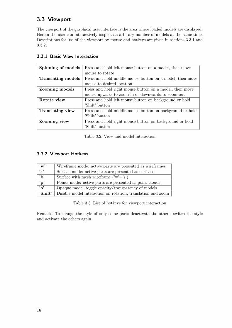
3.3 Viewport

The viewport of the graphical user interface is the area where loaded models are displayed.Herein the user can interactively inspect an arbitary number of models at the same time.Descriptions for use of the viewport by mouse and hotkeys are given in sections 3.3.1 and3.3.2;

3.3.1 Basic View Interaction

Spinning of models Press and hold left mouse button on a model, then movemouse to rotate

Translating models Press and hold middle mouse button on a model, then movemouse to desired location

Zooming models Press and hold right mouse button on a model, then movemouse upwarts to zoom in or downwards to zoom out

Rotate view Press and hold left mouse button on background or hold’Shift’ button

Translating view Press and hold middle mouse button on background or hold’Shift’ button

Zooming view Press and hold right mouse button on background or hold’Shift’ button

Table 3.2: View and model interaction

3.3.2 Viewport Hotkeys

’w’ Wireframe mode: active parts are presented as wireframes

’s’ Surface mode: active parts are presented as surfaces

’b’ Surface with mesh wireframe (’w’+’s’)

’p’ Points mode: active parts are presented as point clouds

’o’ Opaque mode: toggle opacity/transparency of models

’Shift’ Disable model interaction on rotation, translation and zoom

Table 3.3: List of hotkeys for viewport interaction

Remark: To change the style of only some parts deactivate the others, switch the styleand activate the others again.

16

3.4 Data Panel

The data panel organizes geometry and quantity releated information. It is devided ina ’Mesh’ section 3.4.1 where opened source and target meshes with their parts are listedand a ’Quantity’ section 3.4.2 where quantities for mapping and validation are managed.

3.4.1 Mesh Panel

Figure 3.8: Mesh Panel

The ’Mesh’ panel can be used to manage models as well as their relative postition to eachother. Here, each loaded model is assigned to the list of source or list of target models.For each model, a so call model tree gives an overview about the model and its subsetpartitions. Single parts or models can be activated or deactivated for visualization and anunit system can be assigned for each model separately.At the bottom of the ’Mesh’ panel, a form based layout offers different automatic modelalignment options 3.4.1 which can be used to place models before data exchange.

Model and Part Selection

Double clicking on model nameModels are activated or deactivated (for mapping, aligning and visualization)

Double clicking on part nameParts are activated or deactivated (for mapping, aligning and visualization)

Click on triangleCollapse or expand the parts tree

Right click on model namePop up of Models Context Menu

Table 3.4: Part selection options

17

Models Context Menu

On right click on model tree the ’models context menu’ opens.

Figure 3.9: Models Menu

Model InformationShows Information about the mesh topology and quantities

Deactivate PartsDeactivates all parts of model (for mapping, aligning and visualization)

Activate PartsActivate all parts of model (for mapping, aligning and visualization)

Swap PartsDeactivates all activated and activates all deactivated parts

Overwrite Unit SystemDuring reading all data (point coordinates, thickness, stress..) is transformed toSI-units. During writing all data is transformed back to the original unit system.Use this option if the first guess of the unit system was wrong.

DeleteRemoves mesh from the GUI and database

Automatic Positioning

Figure 3.10: Automatic model alignment tools

A common problem in data mapping between different simulation models is the use ofvarying local coordinate systems. Here, the models might not have the same spaticallocation in a common coordinate system. Hence, for a position-dependent neighborhood

18

computation, both models need to be aligned in a preprocessing step. This alignment stepcan be done using the automatic positioning features in MpCCI Mapper (c.f. table 3.11).

Remember current position for mapping and validation

Set model positions to last remembered position.

Rough Align:Used to bring equal meshes close to each other.

Fine Align:Align meshes for mapping. Can be used several times to improve the result.

Symmetric Align:Used if one of the models uses axes symmetry

Mirror Geometry:Mirrors all active modelsWarning: Mirroring is applied to the geometry. When saving the mappingresults of a mirrored target, the mirrored geometry is written to the output file.

Save current positions to a file:1. It is possible to store the transformations in Mapper format (*.trf)2. Export target mesh nodes in current postition in LSDyna keyword format3. Export source mesh nodes in current postition in LSDyna keyword format4. Export target mesh position using INCLUDE TRANSFORM LSDyna card5. Export source mesh position using INCLUDE TRANSFORM LSDyna card

Load transformation from a file:It is possible to read the transformation of a target to a source modelin MpCCI Mapper format. Transformation needs to be initialized with keyword”*transformation”. Declation of the transformation begins with a new lineand is read linewise; entries need to be separated by blanks.Note: All active targets will be transformed.

Figure 3.11: List of available automatic positioning methods.

If the transformation of both coordinate systems are know, a manual setup of the MpCCIMapper transformation file can be done in he following way:

Example Transformation

If A = (aij)i,j=1,..,3 is the rotation matrix of a model in the 3-dimensional space and T =(ti)i=1,..,3 the translation vector we have the transformation Q in homogenous coodinates

Q =

a11 a12 a13 t1a21 a22 a23 t2a31 a32 a33 t30 0 0 1

*transformation = -3.289344e-05 -1.000000e-00 1.079831e-06 2.674954e-04

5.307190e-04 1.062373e-06 9.999999e-01 -3.006939e-01

19

-9.999999e-01 3.289400e-05 5.307189e-04 1.028435e+00

0.000000e+00 0.000000e+00 0.000000e+00 1.000000e+00

20

3.4.2 Quantity Panel

The ’Quantity’ panel, as second entry of the data panel, lists up quantities which arecurrently loaded inside MpCCI Mapper and are available for mapping to other models orfor validation purpose.

Mapping Quantity Selection

In the ’Mapping’ section (c.f. figure 3.12) of the quantity panel a list of all availablequantities is shown. By default, all present quantities are set active for mapping. If only asubset should be used, unwanted transfer quantities can be deactivated in the list overviewby direct user interaction 3.4.2 or semi-automatic using the quantity context menu 3.4.2.

Figure 3.12: Selection of quantites for mapping

Left ClickSelect/deselect quantity for visualization of values as contour plot

Double (Left or Mid) ClickActivate/deactivate quantity for mapping (black/grey letters)

Right ClickOpen quantity dialog box 3.4.2

DeselectShow parts

Table 3.5: Mapping quantity interaction

Remark:

Averaged values of all element integration points are used for element based data visuali-sation. This may lead to varying color display if source and target have different numberof integration points.

21

Quantity Context Menu

By right clicking on a quantity name the quantity context menu opens. Here, automaticselection and deselection operations on quantities can be done or additional informationon especially tensor data can be requested for display (c.f. table 3.4.2).

Figure 3.13: Overview of the Quantity Context Menu

ActivateActivate quantity for mapping

DeactivateDeactivate quantity for mapping

Activate All QuantitiesActivates all defined quantities for mapping

Deactivate All QuantitiesDeactivates all quantities

Swap All QuantitiesActivates currently deactivated quantities, deactivates currently activated quantities

Display TensorsShow principal axes of a tensor quantity

Hide TensorsHides principal axes of a tensor quantity

RenameAssign a new name for selected quantity

Plot DistributionShows a percentual distribution of selected quantity per mesh in a 2D plot 3.5.3

Table 3.6: Quantity Dialog Options

22

3.4.3 Quantity Validation

Figure 3.14: Quantity Validation Panel

The Validation panel is designed for validating mapped and non-mapped quantity dataon given source and target meshes. By default all quantities defined on source and targetmodel will be used during validation process. For individual configuration of quantitiesuse the right click context menu 3.15.Note: Validation functionality can also be used to compare nonmapped quantities.

DISTANCE ELEMENTShows the association distance of the current mapping position. The distance of thevisible target parts to the visible source parts is calculated.

DISTANCE NODALShows the distance to the next node of the current mapping position. The distanceof the visible target parts to the visible source parts is calculated.

Scalar QuantitiesDuring validation of a scalar quantity three validation quantities are created. First,a quantity containing the result of mapping information back from target to sourcemesh is generated having extension “ BACKMAPPED”. Second, using base and“ BACKMAPPED” quantity, absolute difference values are computed and storedhaving “ ABSOLUTE DIFFERENCE” extension. Third, using base and“ ABSOLUTE DIFFERENCE” quantity absolute relative difference values are com-puted and stored having “ RELATIVE DIFFERENCE” extension.

Vector QuantitiesDuring validation of a scalar quantity three validation quantities are created. First,a quantity containing the result of mapping information back from target to sourcemesh is generated having extension “ BACKMAPPED”. Second, using base and“ BACKMAPPED” quantity, absolute difference values are computed per vectorcomponent and stored having “ ABSOLUTE DIFFERENCE” extension. Third, us-ing base and “ BACKMAPPED” quantity, the angular deviation in degree is com-puted and stored having “ DIRECTION DIFFERENCE” extension.

Tensor QuantitiesDuring validation of a scalar quantity three validation quantities are created. First,

23

a quantity containing the result of mapping information back from target to sourcemesh is generated having extension “ BACKMAPPED”. Second, using base and“ BACKMAPPED” quantity, absolute difference of tensor principal values are com-puted and stored having “ MAX PRINCIPAL DIFFERENCE” extension. Third,using base and “ BACKMAPPED” quantity, the angular deviation in degree is com-puted for all principal directions and stored having the extension“ PRINCIPAL DIRECTION DIFFERENCE”.

Figure 3.15: Quantity Validation Dialog

Supplementary to the automatic mode, individual quantity sets can be defined using rightclick optin on validation list and selecting “Validate Quantity” from context menu. Inthe following “Quantity Validation Dialog” 3.15 available quantities can be assigned tovalidation list.

After the (mapping) validation has been performed, a statistical analysis of the obtainedvalidation quantities can be displayed. Here, for each validation quantity the absoluteminimum and maximum as well as the arithmetic mean together with the standard de-viation is computed. At the end, those data is visualized in a tabule report dialog 3.16.Optionally the table result can be exported as comma separated value (*.csv) file.

Figure 3.16: Quantity Validation Report

24

3.5 Postprocessing

3.5.1 Element Information

By pressing the ”element information button” located at the toolbar and picking an el-ement of a mesh in the viewport it is possible to access geometric and (scalar) quantityinformation of this element. As graphical assistance the selected element in bordered inthe visualisation window. The new information window lists:

• Id of selected element

• Type of selected element

• Ids of nodes forming the element

• Scalar value on element / each node are show and can be edited

• Current unit of active quantity

25

3.5.2 Slice Model and Plot

Pressing the ”slice model plot“ of the toolbar an interactive plane widget will be shownin the viewport. By manual interaction with the plane normal arrow, the position anddirection of a slice through the model can be defined.

x-axis: unwinded length of the traversey-axis: interpolated quantity value

Basic interactions on plane widget

• Recompute values by click on plane surface

• Rotate plane normal by left click on arrow and mouse movement

• Translate normal rotation point by middle click on ball and manual positioning

• Translate plane by either left or middle click on plane

• Shrink or extend bounding box by right click and mouse movement

For every position update of the plane surface the MpCCI Mapper tries to compute a socalled length plot corresponding to the quantity distribution. Thereby element edges areintersected with the plane representation and nodal or elemental scalar data is interpo-lated on the intersection points. Then a traverse is computed that represents the geometryalongthe defined plane.

Notes and restriction

Multiple models can simultaniously be cut using the slice functionality; multiply plots getan x-axis offset corresponding to the geometric distance of the traverse starting point.Plot axis can get manually scaled at the end of the axis (cursor changes).

3.5.3 Quantity Plot

To study the relative distribution of a quantity, it’s distribution on a percentage basis canbe visualized as 2D-plot. First, select desired quantity in ”Mapping“ or ”Validation“ tab

26

of the quantity panel. On right-click the quantity name the context menu opens 3.4.2,then select ”Plot Quantity“ option in list.

Figure 3.17: Distribution of a certain quantity

The value range interval will be devided in ten equally spaced sub-intervals and the relativefrequency of data points in the sub-interval range is plotted for each model separately.

3.6 Mapping - Theory of Algorithms in MpCCI Mapper

The discrete mapping problem for a set of N known data points, described as a list oftuples [(x1, u1), (x2, u2), ..., (xN , uN )], where xi denote points in the 3-dimensional spaceand ui the corresponding values of an unknow function u(x) : x → R, x ∈ D ⊂ R3

Goal of the interpolation problem is to find a function u to be ”smooth“ and to be exactu(xi) = ui.

3.6.1 Euclidean inverse distance weighted k-nearest

A general form of finding an interpolating function u at a given point x based on samplesu(xi) = ui for i = 1,..., N is the Euclidean Inverse Distance Weighting method

u(x) =

∑N

i=1 wi(x)ui∑Ni=1 wi(x)

, if ||x− xi|| > 0 for all i,

ui, if ||x− xi|| = 0 for some i

where

wi(x) =1

||x− xi||p

and p is a positive real number, called the power parameter. As the interpolation functiondepends u on all data tuples, its evaluation gets more and more time consuming withincreasing number of N . By construction of Inverse Distance Weighting, the influence -meaning the weight - of one data pair (xi, ui) decreases exponentially with the Euclideandistance to xi.Utilizing the exponential decrease of the weighting function, the above interpolationscheme can be modified by the k-nearest approach

wi(x) =

{1

||x−xi||p , for those indexes i having the k-th minimal distance to x

0, else

27

3.6.2 Log-Euclidean weighted k-nearest

The exponential of a matrix A is defined by

exp(A) =∞∑i=1

An

n!.

To a given matrix A, another matrix B is said to be the matrix logarithm of A ifexp(B) = A is satisfied.Log-Euclidean metric for symmetric positive definite (spd) matrices

dist(S1, S2) = ||log(S1)− log(S2)||

builds an isomorphism (the algebraic structure of a space is conserved) and is an isometry(distances are conserved) between the space of spd matrices and the Euclidean space.Having a set of N tensors S1, ..., SN with arbitary positive weights w1, ..., wN we canfomulate the Log-Euclidean Frechet mean mean of N tensors by

E(S1, ..., SN ) = exp(

N∑i=1

wilog(Si))

A comparison of the Euclidean and the Log-Euclidean interpolation result of tensors isillustrated in figure 3.18 1.

Figure 3.18: Bilinear interpolation of 4 tensors at the cornersof a grid. Left figure: Eu-clidean interpolation Right figure: Log-Euclidean interpolation.

1Images from Fast and Simple Calculus on Tensors in the Log-Euclidean Framework, Vincent Arsigny,Pierre Fillard, Xavier Pennec, and Nicholas Ayache

28

3.7 Mapping with Mapper

A complete mapping cycle between one source and one target model can be done withjust a few clicks. The following complete mapping and validation workflow illustrates thetypical use of MpCCI Mapper tool. Most of the described steps are optional and maydepend on the models and detail of mapping analysis.

Complete Mapping and Validation Workflow

1. Load a source mesh

2. Load a target mesh

3. Switch to mesh panel (optional)

4. Select source and target mesh parts that shall be used for mapping (optional)

5. Align models (optional)

6. Switch to quantity mapping panel (optional)

7. Select quantities which shall be mapped on target (optional)

8. Press mapping button

9. Switch to quantity validation panel (optional)

10. Press validation button for quantity validation (optional)

11. Save target to file

Restrictions:

1. Only quantities are mapped that are available on the source and can be created (ifnot present) on target.

2. No iterative mapping is supported. If you want to map several sources on one targetyou need to map all at the same time.

3. Mapping solid to shell models requires only one source and one target mesh.

4. Integral values cannot be conserved.

5. Out of plane integration rules are defined for Gauss up to 16, Lobatto up to 16,Trapezodial up to 15, Simpson up to 9 integration points.

6. For stresses only nearest data point should be used (c.f. Mapping Parameter Section3.1.2).

29

3.8 Batch Mode

MpCCI Mapper allows direct loading, mapping of models and result export via programargument list. The required file readers are automatically detected by file extension.By default the mapping in batch mode does require same local coordinate system forsource and target model. In cases where the automatic alignment tools of MpCCI Mapper(c.f. 3.4.1) produces an acceptable alignment, these automatic positioning can be used inbatch as well. If automatic alignment does not work, it is possible to use exported modeltransformation from manual alignment.List of MpCCI Mapper argument list options:

-noguiEnable batch mode of MpCCI Mapper

-csv2dynaUse Autoform CSV output to LSDyna keyword conversion tool

-csv2vtkUse CSV to VTK legacy conversion tool

-disablestressDisable mapping of quantity STRESS

-maximalsearchdistanceDefine the maximal search distance parameter (in model length unit) (c.f. 3.1.2)

-configfileOption to define program settings based on configuration file (c.f. 3.8.5)

-helpThis screen

List of MpCCI Mapper arguments for automatic alignment:

-alignEnable automatic (coarse + fine) model alignment

-coarsealignEnable coarse model alignment

-finealignEnable fine model alignment

-inversealignEnable automatic (coarse + fine) model alignment interchanging source and targetmodel

-inversecoarsealignEnable coarse model alignment interchanging source and target model

-inversefinealignEnable fine model alignment interchanging source and target model

-applytransformEnable model alignment using predefined transformation matrix (c.f. 3.4.1)

30

3.8.1 Batch on Linux Cluster

The graphical user interface of MpCCI Mapper is based on the QT GUI-Toolkit. Itsimplementation on Linux does require an active X Window System framework even ifthe program is running in batch. Normally, Linux cluster compute nodes do not allowthe execution of graphical applications using X Window System. Therefore exist virtualdisplay server, e.g. Xvfb (X virtual framebuffer), implementing the X11 display serverprotocol. Xvfb performs all graphical operations in virtual memory without showing anyscreen output.Before execution of MpCCI Mapper in a shell script on a cluster compute node, a virtualdisplay server can be started by adding the lines

Xvfb :1 &

export DISPLAY=:1

previous to the mapper.exe program call.

3.8.2 Examples

MpCCI Mapper examples using automatic model loading, mapping and result export:

1. mapper.exe source_file

Starts GUI and loads source_file as source model into MpCCI Mapper .

2. mapper.exe source_file target_file

Starts GUI and loads source_file as source model and target_file as target modelinto MpCCI Mapper and maps all defined quantities from source to target.

3. mapper.exe source_file target_file result_file

Same as 2); the mapped results are then exported into result_file in the default exportformat of target_file.

3.8.3 Batch Mode Example

To perform an automatic model import and mapping in batch MpCCI Mapper add the-nogui option as first argument:

4. mapper.exe -nogui source_file target_file result_file

Same as 3) but the MpCCI Mapper GUI is disabled during the whole process.

5. mapper.exe -nogui -config config_file source_file target_file result_file

Same as 4) but the MpCCI Mapper GUI parameter are set using configuration file.

3.8.4 Alignment Examples

To make use of automatic positioning add one of the options -align, -coarsealign,-finealign or their inverse to argument list, e.g

2b. mapper.exe -align source_file target_file

3b. mapper.exe -finealign source_file target_file result_file

31

4b. mapper.exe -nogui -align source_file target_file result_file

3.8.5 Batch Configuration File

Beside starting the MpCCI Mapper in batch with additional process control commands,the complete mapping setup can be specified using a text based configuration file.

*optionAlignDefine automatic model alignment method (same as the options in 3.8)Value Description

none Models are aligned (Default)-align Enable automatic (coarse + fine) model alignment-coarsealign Enable coarse model alignment-finealign Enable fine model alignment-inversealign Enable automatic (coarse + fine) model alignment interchanging

source and target model-inversecoarsealign Enable coarse model alignment interchanging source and target

model-inversefinealign Enable fine model alignment interchanging source and target

model

*optionTransformationDefine transformation file for model alignment (same as ”-applytransform“ in 3.8)Value Description

none defaultGlobal Path To File/transform.trf

*optionMappingDefaultDefine parameter ”Default“ in Mapping Settings 3.1.2Value Description

4 Default1-8 Specify number of data points to use for interpolation

*optionMappingStressOrHistoryDefine parameter ”STRESS/HISTORY“ in Mapping Settings 3.1.2Value Description


*optionMappingOrientationsDefine parameter ”Orientations“ in Mapping Settings 3.1.2Value Description


*optionMappingMaximalSearchDistanceDefine parameter ”Maximal Search Distance“ in Mapping Settings 3.1.2Value Description

-1 No maximal search distance (Default)d > 0. Maximal search distance d should be used

32

*optionMappingMATFEMSettingsEnable special handling of LSDyna history variables when mapping a MATFEM GenYld- CrachFEM result fileValue Description

0 Disabled (Default)1 Enabled

*optionReaderDynaMAT249Active automatic transformation of ply orientation for history variables of LSDynaMAT 249 4.8.4Value Description

0 Disabled (Default)1 Enabled

*optionWriterDynaOutputDefine the mode output files for LSDyna are writtenValue Description

0 Single and multiple file are written (Default)1 Single file only is written-1 Multiple files only are written

*optionWriterDynaMAT58FiberModeAutomatic transformation of ply orientation into MAT 58 4.8.4Value Description

0 Align element coordinate system using fiber 1 (Default)1 Align element coordinate system congurent bisectrix

*optionWriterDynaOrientationToHistoryDefine how variable ORIENTATION TENSOR from molding simulation is handled onLSDyna file exportValue Description

0 Disabled (Default), ELEMENT SOLID ORTHO is writtenfrom ORIENTATION TENSOR 4.8.5

1 Enabled, generate MATFEM GenYld - CrachFEM history variables

*optionDiableStressSpecial flag to disable quantity STRESS for mappingValue Description

0 Map quantity STRESS (Default)1 Disable quantity STRESS for mapping

*optionMappingQuantityDefine a list of quantities to map from source to target

Value Description

-1 Map all quantities (Default)#N ”Quant 1“ ... Map only the N quantities defined by named list

Example of a configuration file to map only ”THICKNESS“ and ”PLASTIC STRAIN“using automatic model alignment:

#comment line

*optionAlign

-align

*optionTransformation

none

*optionDiableStress

0 # 0 = off 1 = on

33

*optionMappingDefault

4 # 1 to 8 points

*optionMappingStressOrHistory

4 # 1 to 8 points

*optionMappingOrientations

1 # 1 to 8 points

*optionMappingMaximalSearchDistance

-1. # Only relevant if value greater 0.

*optionMappingThicknessInterpolation

1 # 0 = off 1 = on

*optionMappingMATFEMSettings

0 # 0 = off 1 = on

*optionReaderDynaMAT249

0 # 0 = off 1 = on

*optionWriterDynaOutput

1 # [-1 / 0 / 1] (Split File / Split and Combined Files / Combined File)

*optionWriterDynaMAT58FiberMode

1 # 0 = align X 1 = congruent

*optionWriterDynaOrientationToHistory

1 # 0 = off 1 = on

*optionMappingQuantity

2 "THICKNESS" "PLASTIC_STRAIN"

34

4 Solver Formats

4.1 Abaqus

4.1.1 File Format

Abaqus Input Deck (*.inp) is supported for reading and writing.

The model can consist of serveral *PART definitions but requires unique node id assign-ments. For example having two *PART definitions ”A”, nodes numbered from 1 to 100,and ”B”, nodes numbered from 1 to 80, will lead to an error due to double defined node ids.

Thus, a renumbering of node ids can be performed using Abaqus CAE.

• Import your model file in Abaqus CAE

• Create a new Job from imported model

• Right-Click on the created Job entry and select ’Write Input’

In MpCCI Mapper multiple instances of a *PART is not supported.

An element-based *SURFACE defintion is required for surface coupling.Abaqus/CAE: Create a surface using the Surfaces tool. See also “13.7.6 Using sets andsurfaces in the Assembly module” in the Abaqus/CAE User’s Manual. You can also usesurfaces defined in the Part module.Input File: A surface is created with *SURFACE, NAME=<surface name>, TYPE=ELEMENT,see section 2.3.3 Defining element-based surfaces” of the Abaqus Analysis User’s Manual.

4.1.2 Element Types

Shells

MpCCI Mapper supports reading the following shell element types: S4, S4R, S4RS, S4RS,S3, S3R, S3RS

Solids - Surface Definition

MpCCI Mapper supports reading *SURFACE definition of the following 3D solid elements:DC3D4, C3D4, DC3D5, C3D5, DC3D6, C3D6, DC3D8, C3D8, DC3D10, C3D10

35

4.1.3 Transferable Quantities

Quantity Read Write

THICKNESS x xSTRESS x xPLASTIC STRAIN x xPRESSURE - xORIENTATION - xPLY VECTOR - x

Quantity Boundary Condition Type

THICKNESS *NODAL THICKNESS

*DISTRIBUTION,LOCATION=ELEMENT,NAME=SHELL_THICKNESS_DIST

STRESS *INITIAL CONDITIONS,TYPE=STRESS

PLASTIC STRAIN *INITIAL CONDITIONS,TYPE=HARDENING

PRESSURE *DLOAD

ORIENTATION *ORIENTATION

*DISTRIBUTION TABLE using COORD3D, *DISTRIBUTIONPLY VECTOR *SHELL SECTION, , COMPOSITE

*DISTRIBUTION TABLE, *DISTRIBUTION and *ORIENTATION

4.1.4 Output Files

To use the files in your input file include them via the ”INCLUDE” keyword. To registerthe nodal thickness add the ”NODAL THICKNESS” option to the relevant ”SHELLSECTION” entriese.g.:*SHELL SECTION,NODAL THICKNESS,ELSET=...,SECTION INTEGRATION=SIMPSON,MATERIAL=...

To register element thickness use the ”DISTRIBUTION TABLE” option, e.g.*SHELL SECTION,SHELL THICKNESS=SHELL_THICKNESS_DIST,ELSET=...,SECTION INTEGRATION=...

36

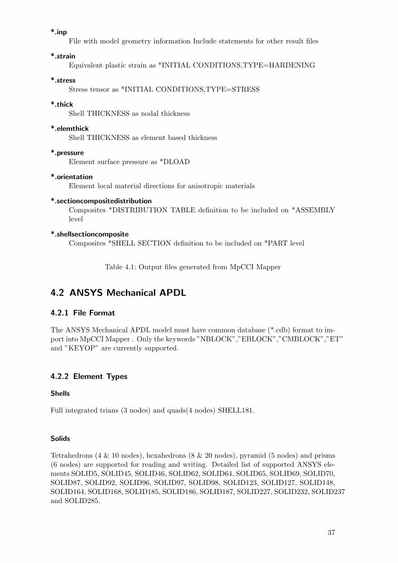
*.inpFile with model geometry information Include statements for other result files

*.strainEquivalent plastic strain as *INITIAL CONDITIONS,TYPE=HARDENING

*.stressStress tensor as *INITIAL CONDITIONS,TYPE=STRESS

*.thickShell THICKNESS as nodal thickness

*.elemthickShell THICKNESS as element based thickness

*.pressureElement surface pressure as *DLOAD

*.orientationElement local material directions for anisotropic materials

*.sectioncompositedistributionComposites *DISTRIBUTION TABLE definition to be included on *ASSEMBLYlevel

*.shellsectioncompositeComposites *SHELL SECTION definition to be included on *PART level

Table 4.1: Output files generated from MpCCI Mapper

4.2 ANSYS Mechanical APDL

4.2.1 File Format

The ANSYS Mechanical APDL model must have common database (*.cdb) format to im-port into MpCCI Mapper . Only the keywords ”NBLOCK”,”EBLOCK”,”CMBLOCK”,”ET”and ”KEYOP” are currently supported.

4.2.2 Element Types

Shells

Full integrated trians (3 nodes) and quads(4 nodes) SHELL181.

Solids

Tetrahedrons (4 & 10 nodes), hexahedrons (8 & 20 nodes), pyramid (5 nodes) and prisms(6 nodes) are supported for reading and writing. Detailed list of supported ANSYS ele-ments SOLID5, SOLID45, SOLID46, SOLID62, SOLID64, SOLID65, SOLID69, SOLID70,SOLID87, SOLID92, SOLID96, SOLID97, SOLID98, SOLID123, SOLID127, SOLID148,SOLID164, SOLID168, SOLID185, SOLID186, SOLID187, SOLID227, SOLID232, SOLID237and SOLID285.

37


Quantities THICKNESS, TEMPERATURE, STRESS, STRAIN, PLASTIC STRAIN, PRES-SURE and ORIENTATION TENSOR are supported for mapping and writing. Boudarycondition type INISTATE use defaut coordinate system identifier 0.


THICKNESS Tabular $NodeId $Value

TEMPERATURE BF, ,TEMP

STRESS INISTATE, SET, DTYP, S

STRAIN INISTATE, SET, DTYP, EPEL

PLASTIC STRAIN INISTATE, SET, DTYP, EPPL

PRESSURE SFE,,,PRES

ORIENTATION TENSOR Moldflow xml format, Digimat *.dofWELD LINE Element set or Digimat *.dofDISPLACEMENTS nblock coordinate with applied displacement

38

4.3 AutoForm R4 converter

MpCCI Mapper command to convert exported CSV format reads as follows

> mapper.exe -csv2dyna FILE 1 FILE 2 FILE 3 FILE 4

where each file in argument list needs to contain parameters as specifyed in table 4.2.

File Description

FILE 1 * NodeData Thickness containing nodal coordinates and idsFILE 2 * ElementData Thickness containing element topology and thicknessFILE 3 * ElementData Plastic Strain containing element topology plastic strainFILE 4 Result File Name

Table 4.2: AutoForm converter parameter list

Required CSV format per output file:

1. * NodeData Thickness:

Node Idx,XCoord,YCoord,ZCoord,,Info

2. * ElementData Thickness:

Element Idx,Node Idx 1,Node Idx 2,Node Idx 3,Thickness,,Info

3. * ElementData Plastic Strain (5 points over thickness):

Element Idx,Node Idx 1,Node Idx 2,Node Idx 3,Plastic Strain Layer -2,Plastic StrainLayer -1,Plastic Strain,Plastic Strain Layer 1,Plastic Strain Layer 2,,Info

39

4.4 Cadmould

4.4.1 File Format

Cadmould geometry file *.cfe is supported. The file contains the element definitions,the node coordinates, the number of nodes and elements and an identifier if it is a surfacemesh or a midplane mesh. MpCCI Mapper can import both midplane and surface meshes.Surface meshes consist of pairs of triangles which are internally converted into a layeredprism mesh. Midplane meshes consist of triangular shell elements. As result format binary*.car files containing ORIENTATION TENSOR information can be read.


Quantity Read Write

THICKNESS x -ORIENTATION TENSOR x -

4.5 Indeed

4.5.1 File Format

For code Indeed reading of ASCII result file (*.asc) and geometry file (*.inc) is supported.

4.5.2 Element Types

The 6- and 8-node Crisfield-Solid-Shell elements are supported for reading.


Quantity Read Write

THICKNESS x -STRESS x -PLASTIC STRAIN x -

40

4.6 MSC Simufact

4.6.1 File Format

All MSC.Simufact products, Additive, Forming and Welding, offer a configurable resultexport utilizing the Universal File format (*.unv), which is fully supported by MpCCIMapper .

4.6.2 Element Types

MpCCI Mapper supports reading of all element types available in MSC Simufact product.The interface comprises reading solid, thick shell and shell elements.


Both, nodal and element integration point results can be read from MSC.Simufact Uni-versal files. The data in imported in SI units. The following list of output variables isautomatically handeled as MpCCI Mapper quantitites:

Quantity Read Write

THICKNESS x -STRESS x -PLASTIC STRAIN x -TEMPERATURE x -DISPLACEMENTS x -

41

4.7 Forge

4.7.1 File Format

The Universal File format (*.unv), which can be exported via the IDEAS export interfacein GLPre, is supported by MpCCI Mapper .

4.7.2 Element Types

Shells

Full integrated trians (3 & 6 nodes) and quads(4 nodes) are supported for reading.

Solids

Tetrahedrons (4 & 10 nodes), hexahedrons (8 & 20 nodes) and prisms (6 nodes) aresupported for reading.


In general nodal based (card format 55), element based (card format 56) and generalcard format 2414 quantities (nodal or element based) can be read from Universal Fileformat. Variables TEMPERATURE and STRESSTENSOR are automatically detectedand assigned as MpCCI Mapper quantities TEMPERATURE and STRESS.

42

4.8 LSDyna

4.8.1 File Format

LSDyna keyword format (*.k,*.key,*.dyn,*dynain) is supported for reading and writing.

4.8.2 Element Types

*ELEMENT SHELL Card

Full integrated trians (3 nodes) and quads(4 nodes). Arbitrary out of plane integrationtypes up to 16 integration points out of plane.

*ELEMENT SOLID Card

Tetrahedrons (4 & 10 nodes), hexahedrons (8 nodes) and prisms (6 nodes) are supportedfor reading and writing. Element formulations -2, -1, 1, 2, 10, 13, 15, 16 and 115 formsolid section can be used for quantity generation.


Quantity Read Write Boundary Condition or Element Card

THICKNESS x x *ELEMENT_SHELL_THICKNESS

STRESS x x *INITIAL_STRESS_SHELL

x x *INITIAL_STRESS_SOLID

STRAIN x x *INITIAL_STRAIN_SHELL

x x *INITIAL_STRAIN_SOLID

PLASTIC STRAIN x x *INITIAL_STRESS_SHELL


HISTORY Variables x x *INITIAL_STRESS_SHELL


ORIENTATION TENSOR - x *INITIAL_STRESS_SHELL

x x *ELEMENT_SOLID_ORTHO

- x *INITIAL_STRESS_SOLID

ELEMENT SHELL BETA x x *ELEMENT_SHELL_THICKNESS

TEMPERATURE - x *INITIAL_TEMPERATURE_NODE

Table 4.3: MpCCI Mapper quantities in LSDyna solver format

4.8.4 Composite Material Model Features

For LSDyna Version R 10 MpCCI Mapper supports direct mapping of locally orthotropicmaterial axes from *MAT REINFORCED THERMOPLASTIC (*MAT 249) to*MAT LAMINATED COMPOSITE FABRIC (*MAT 58). Therefor direction of fibers,stored in certain HISTORY Variables, are gathered in separated vector quantites:

Quantity Name HISTORY Variable Comment

PLY VECTOR 1 POSTV dependent Direction 1st fiber (global coordinates)PLY VECTOR 2 POSTV dependent Direction 2nd fiber (global coordinates)

Table 4.4: MpCCI Mapper quantities for composites.

43

4.8.5 Injection Molding Features

The fiber ORIENTATION TENSOR result shows the probability of fiber alignment inthe specified principal direction at the end of a injection molding process. Depending onthe degree of orientation MpCCI Mapper can classify and export 15 different placeholdermaterial cards as well as section solid assignments for solid elements. For each solid elementlocal material axes are defined using *ELEMENT SOLID ORTHO card. For material #1a *MAT ELASTIC template and for material 2-15 a *MAT ANISOTROPIC ELASTICtemplate is written to output files.

Id Material Title SECTION SOLID TITLE Comment

1 MATERIAL ISOTROPIC PART ISOTROPIC a11 = a22 = a33 = 0.332 MATERIAL 0 4 0 3 0 3 PART 0 4 0 3 0 3 a11 = 0.4, a22 = 0.3, a33 = 0.33 MATERIAL 0 4 0 4 0 2 PART 0 4 0 4 0 2 a11 = 0.4, a22 = 0.4, a33 = 0.34 MATERIAL 0 5 0 3 0 2 PART 0 5 0 3 0 2 a11 = 0.5, a22 = 0.3, a33 = 0.25 MATERIAL 0 5 0 4 0 1 PART 0 5 0 4 0 1 a11 = 0.5, a22 = 0.4, a33 = 0.16 MATERIAL 0 5 0 5 0 0 PART 0 5 0 5 0 0 a11 = 0.5, a22 = 0.5, a33 = 0.07 MATERIAL 0 6 0 2 0 2 PART 0 6 0 2 0 2 a11 = 0.6, a22 = 0.2, a33 = 0.28 MATERIAL 0 6 0 3 0 1 PART 0 6 0 3 0 1 a11 = 0.6, a22 = 0.3, a33 = 0.19 MATERIAL 0 6 0 4 0 0 PART 0 6 0 4 0 0 a11 = 0.6, a22 = 0.4, a33 = 0.010 MATERIAL 0 7 0 2 0 1 PART 0 7 0 2 0 1 a11 = 0.7, a22 = 0.2, a33 = 0.111 MATERIAL 0 7 0 3 0 0 PART 0 7 0 3 0 0 a11 = 0.7, a22 = 0.3, a33 = 0.012 MATERIAL 0 8 0 1 0 1 PART 0 8 0 1 0 1 a11 = 0.8, a22 = 0.1, a33 = 0.113 MATERIAL 0 8 0 2 0 0 PART 0 8 0 2 0 0 a11 = 0.8, a22 = 0.2, a33 = 0.014 MATERIAL 0 9 0 1 0 0 PART 0 9 0 1 0 0 a11 = 0.9, a22 = 0.1, a33 = 0.015 MATERIAL 1 0 0 0 0 0 PART 1 0 0 0 0 0 a11 = 1.0, a22 = 0.0, a33 = 0.0

Table 4.5: *ELEMENT SOLID ORTHO output generated by MpCCI Mapper from amapped ORIENTATION TENSOR.

4.8.6 Output Files

*.key File with model *NODE definitionInclude statements for *.key.thick and *.key.stressstrain

*.key.thick Model *ELEMENT definition with THICKNESS

*.key.stressstrain STRESS, STRAIN, PLASTIC STRAIN and HISTORY Variables

* complete.key Combinend *.key,*.key.thick and *.key.stressstrain output

* with displacements.key Optional file containing morphed coordinates when mappingsolid to shell

Table 4.6: Output files generated from MpCCI Mapper

Historyvariables

MpCCI Mapper allows a redefinition of the output sequence of history variables via ASCII-based configuration file over the specific environment variable or via the file writer settingsdialog 3.1.2. Using the environment variable option, a user has to specify the variable

LSDYNA_HISTORY_CONFIGURATION_FILE=Global_Path_To_File/File

44

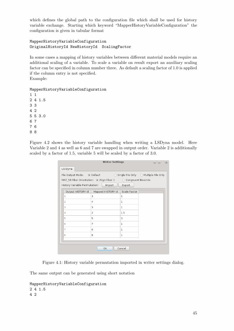
which defines the global path to the configuration file which shall be used for historyvariable exchange. Starting which keyword “MapperHistoryVariableConfiguration” theconfiguration is given in tabular format

MapperHistoryVariableConfiguration

OriginalHistoryId NewHistoryId ScalingFactor

In some cases a mapping of history variables between different material models require anadditional scaling of a variable. To scale a variable on result export an auxiliary scalingfactor can be specified in column number three. As default a scaling factor of 1.0 is appliedif the column entry is not specified.Example:


1 1

2 4 1.5

3 3

4 2

5 5 3.0

6 7

7 6

8 8

Figure 4.2 shows the history variable handling when writing a LSDyna model. HereVariable 2 and 4 as well as 6 and 7 are swapped in output order. Variable 2 is additionallyscaled by a factor of 1.5, variable 5 will be scaled by a factor of 3.0.

Figure 4.1: History variable permutation imported in writer settings dialog.

The same output can be generated using short notation


2 4 1.5

4 2

45

5 5 3.0

6 7

7 6

If the new history id is set to “0”, the variable is set to zero for all integration points andthus treated as empty.

Figure 4.2: History variable permutation imported in writer settings dialog.

Element formulation and integration scheme

Figure 4.3: Redefinition of Elform and through thickness integration scheme

If the LSDyna model is used as target model, MpCCI Mapper supports a check and redef-inition of shell element formulation and through thickness integration rule (and number ofpoints though thickness) for each shell section within the model. Using right-click optionon target model name in “Target Models” tree 3.4.1, then selecting “Overwrite Integra-tion Rule” an integration types dialog opens 4.3. Here, a default shell section integrationformula is given as well for each shell section within the model an additional data row tochange element fomulation (reduced of fully integrated) as well as the number of integra-tion points though thickness.

46

Note: If element formulation of the number of integration points though thickness ischanged, all defined quantities of the model will be deleted. To obtain data on specifiedelement formulation / number of integration points please re-run mapping step.

47

4.9 Marc / COPRA FEA

4.9.1 File Format

MpCCI Mapper supports reading of ASCII based MSC Marc result format (*.t19). Bydefault MSC Marc does export binary .t16 files only which are not supported. To requestan ASCII .t19 select the relevant Job in MSC Mentat Preprocessor, and go ’Job Properties’→ ’Job Results’ → ’Post File’ and activate ’Binary & ASCII’ option. Then, both ASCIIand Binary file will be written during simulation.

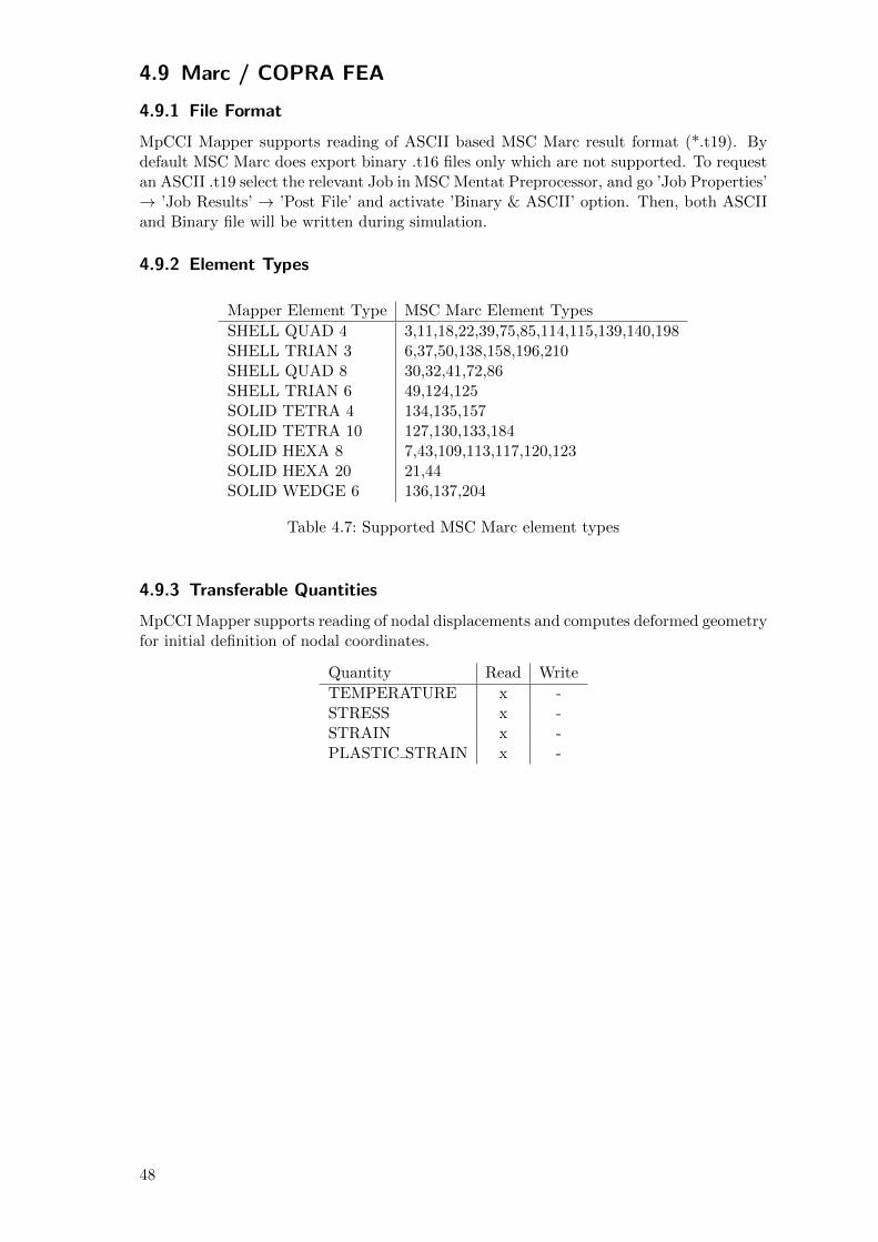
4.9.2 Element Types

Mapper Element Type MSC Marc Element Types

SHELL QUAD 4 3,11,18,22,39,75,85,114,115,139,140,198SHELL TRIAN 3 6,37,50,138,158,196,210SHELL QUAD 8 30,32,41,72,86SHELL TRIAN 6 49,124,125SOLID TETRA 4 134,135,157SOLID TETRA 10 127,130,133,184SOLID HEXA 8 7,43,109,113,117,120,123SOLID HEXA 20 21,44SOLID WEDGE 6 136,137,204

Table 4.7: Supported MSC Marc element types


MpCCI Mapper supports reading of nodal displacements and computes deformed geometryfor initial definition of nodal coordinates.

Quantity Read Write

TEMPERATURE x -STRESS x -STRAIN x -PLASTIC STRAIN x -

48

4.10 Moldflow

4.10.1 File Format

Moldflow geometry file exported to PATRAN neutral (*.pat) is supported. The file con-tains the element definitions and the node coordinates. ORIENTATION TENSOR resultsas generic .xml or PATRAN neutral (*.nod) are supported for reading.


Quantity Read Write

THICKNESS x -ORIENTATION TENSOR x -

4.11 Nastran

4.11.1 File Format

MpCCI Mapper supports reading of ASCII Nastran Bulk data format (*.nas,*.bdf). Nodalcoordinates can be either in long (GRID*) or short (GRID) format. Nastran so called freeformat is not supported.

4.11.2 Element Types

Triangles CTRIA3 and quads CQUAD4 are supported for reading and writing.


Quantity Read Write

THICKNESS x xSTRESS - xPLASTIC STRAIN - xPRESSURE x x


THICKNESS element description card formatSTRESS ISTRSSH for SOL 700 onlyPLASTIC STRAIN ISTRSSH for SOL 700 onlyPRESSURE PLOAD2

49

4.12 PAM

4.12.1 File Format

MpCCI Mapper supports the following native PAM solver ASCII formats:PAMStamp mapping files (*M00-*M99)PAMCrash input deck (*.pc,*.ps)


Full integrated triangles (3 nodes) and quads(4 nodes) with arbitrary out of plane inte-gration number can be read. Only active parts are written into *M00-*M99 format forboth native solver input types.


Quantity Read Write Boundary Condition

THICKNESS x x THICSTRESS x x STRSSTRAIN x x STRNPLASTIC STRAIN x x PLASPRESSURE - x PREFAHV x x HV

4.13 Radioss

4.13.1 File Format

Radioss Result (*Yxxx) Reading and writing is supportedRadioss Result (*.sta) Reading and writing is supportedRadioss Input (*D00, .rad) Reading is supported


Fully integrated and reduced integrated triangles and quads are supported.


Quantity Read Write

THICKNESS x xSTRESS x xPLASTIC STRAIN x x

50

4.14 Sysweld

4.14.1 File Format

*.asc Model information file

*_trans.asc Mechanical or thermal result fileStresses, strain, plastic strain and young modul is extracted.The effectiv plastic strain is extracted from plastic strain.

*_phase.asc Defining names for the phases.

The syntax is that of the sysweld files and looks like this

SYSWELD_PHASE_DEFINITION First line of file is the magic word.BEGIN_PHASEDEF Starting to define the mnemonics1 "MARTENSIT" Name of first phase2 "AUSTENIT" Name of second phase5 "SOMEOTHERUSERDEFINEDPHASE" Name of phase fiveEND_PHASEDEF End of definition statments

Output The files exept the *_phase.asc from above are written or are patched wherevalues have changed.

!! Attention, currently the writer is designed to write the mapped values of a metal formingresult. To keep equlibrium the elastic strains are calculated from the residual stresses. Asonly plastic strains can be written and as the total strain needs to be 0 (displacementsare assumed to be 0) the plastic strain is set to the calculated negative strain values. Theyoung modulus is used to calculate the strains.

51

5 Other Formats

5.1 Argus / Aramis

Argus and Aramis offer a configurable output format which can be imported in MpCCIMapper (*.txt). Thickness information and strain can be imported.

5.1.1 File Format

To define an initial thickness (here 1.00 mm) use following string in file header commentblock:

# Ausgangsblechdicke: 1.00mm

1 2 3 4 5 6 7 8 9 10

s u v x_coord y_coord z_coord phi_1 phi_2 phi_3 %thickness reduction

Table 5.1: Order of Variables required for MpCCI Mapper

5.2 Atos

5.2.1 File Format

The ’Gesellschaft fur Optische Messtechnik’ offers an export plugin that allows geometryand thickness information export in polygon file format (*.ply) which is supported forreading in MpCCI Mapper . This plugin can be received directly from GOM http:

//www.gom.com.

5.3 AutoGrid

5.3.1 File Format

MpCCI Mapper supports AutoGrid *.dat file import for software version 4.1.x.x and4.2.x.x. Thickness and strain can be imported.

5.4 STL

Eighter ASCII or binary STL-files can be imported in MpCCI Mapper using the common*.stl file extension.

52

http://www.gom.com

http://www.gom.com

5.5 VTK

ASCII based VTK legacy files (*.vtk) can be imported in MpCCI Mapper .

5.5.1 Element Types

VTK MpCCI Mapper Comment

VTK TRIANGLE TRIAN 3-node shell elementVTK QUAD QUAD 4-node shell elementVTK QUADRATIC TRIANGLE TRIAN6 6-node shell elementVTK QUADRATIC QUAD QUAD8 8-node shell elementVTK TETRA TETRA 4-node volume elementVTK HEXAHEDRON HEXA 8-node volume elementVTK WEDGE WEDGE 6-node volume elementVTK QUADRATIC TETRA TETRA10 10-node volume elementVTK QUADRATIC HEXAHEDRON HEXA20 20-node volume element

Table 5.2: Translation of VTK elements in MpCCI Mapper

53

6 Thirdparty License Information

6.1 LibQxt

Copyright (c) 2006 - 2011, the LibQxt project. See the Qxt AUTHORS file for a list ofauthors and copyright holders. All rights reserved.

Redistribution and use in source and binary forms, with or without modification, arepermitted provided that the following conditions are met:

• Redistributions of source code must retain the above copyright notice, this list ofconditions and the following disclaimer.

• Redistributions in binary form must reproduce the above copyright notice, this list ofconditions and the following disclaimer in the documentation and/or other materialsprovided with the distribution.

• Neither the name of the LibQxt project nor the names of its contributors may beused to endorse or promote products derived from this software without specific priorwritten permission.

THIS SOFTWARE IS PROVIDED BY THE COPYRIGHT HOLDERS AND CON-TRIBUTORS ”AS IS” AND ANY EXPRESS OR IMPLIED WARRANTIES, INCLUD-ING, BUT NOT LIMITED TO, THE IMPLIED WARRANTIES OF MERCHANTABIL-ITY AND FITNESS FOR A PARTICULAR PURPOSE ARE DISCLAIMED. IN NOEVENT SHALL ¡COPYRIGHT HOLDER¿ BE LIABLE FOR ANY DIRECT, INDI-RECT, INCIDENTAL, SPECIAL, EXEMPLARY, OR CONSEQUENTIAL DAMAGES(INCLUDING, BUT NOT LIMITED TO, PROCUREMENT OF SUBSTITUTE GOODSOR SERVICES; LOSS OF USE, DATA, OR PROFITS; OR BUSINESS INTERRUP-TION) HOWEVER CAUSED AND ON ANY THEORY OF LIABILITY, WHETHERIN CONTRACT, STRICT LIABILITY, OR TORT (INCLUDING NEGLIGENCE OROTHERWISE) ARISING IN ANY WAY OUT OF THE USE OF THIS SOFTWARE,EVEN IF ADVISED OF THE POSSIBILITY OF SUCH DAMAGE.http://libqxt.org [email protected]

6.2 Libtiff

Copyright (c) 1988-1997 Sam Leffler Copyright (c) 1991-1997 Silicon Graphics, Inc.Permission to use, copy, modify, distribute, and sell this software and its documentationfor any purpose is hereby granted without fee, provided that (i) the above copyright noticesand this permission notice appear in all copies of the software and related documentation,and (ii) the names of Sam Leffler and Silicon Graphics may not be used in any advertisingor publicity relating to the software without the specific, prior written permission of SamLeffler and Silicon Graphics.

THE SOFTWARE IS PROVIDED ”AS-IS” AND WITHOUT WARRANTY OF ANYKIND, EXPRESS, IMPLIED OR OTHERWISE, INCLUDING WITHOUT LIMITA-TION, ANY WARRANTY OF MERCHANTABILITY OR FITNESS FOR A PARTIC-

54

ULAR PURPOSE.

IN NO EVENT SHALL SAM LEFFLER OR SILICON GRAPHICS BE LIABLE FORANY SPECIAL, INCIDENTAL, INDIRECT OR CONSEQUENTIAL DAMAGES OFANY KIND, OR ANY DAMAGES WHATSOEVER RESULTING FROM LOSS OFUSE, DATA OR PROFITS, WHETHER OR NOT ADVISED OF THE POSSIBILITYOF DAMAGE, AND ON ANY THEORY OF LIABILITY, ARISING OUT OF OR INCONNECTION WITH THE USE OR PERFORMANCE OF THIS SOFTWARE.

6.3 Libwebp

Copyright (c) 2010, Google Inc. All rights reserved.

Redistribution and use in source and binary forms, with or without modification, arepermitted provided that the following conditions are met:



• Neither the name of Google nor the names of its contributors may be used to en-dorse or promote products derived from this software without specific prior writtenpermission.

THIS SOFTWARE IS PROVIDED BY THE COPYRIGHT HOLDERS AND CONTRIB-UTORS ”AS IS” AND ANY EXPRESS OR IMPLIED WARRANTIES, INCLUDING,BUT NOT LIMITED TO, THE IMPLIED WARRANTIES OF MERCHANTABILITYAND FITNESS FOR A PARTICULAR PURPOSE ARE DISCLAIMED. IN NO EVENTSHALL THE COPYRIGHT HOLDER OR CONTRIBUTORS BE LIABLE FOR ANYDIRECT, INDIRECT, INCIDENTAL, SPECIAL, EXEMPLARY, OR CONSEQUEN-TIAL DAMAGES (INCLUDING, BUT NOT LIMITED TO, PROCUREMENT OF SUB-STITUTE GOODS OR SERVICES; LOSS OF USE, DATA, OR PROFITS; OR BUSI-NESS INTERRUPTION) HOWEVER CAUSED AND ON ANY THEORY OF LIA-BILITY, WHETHER IN CONTRACT, STRICT LIABILITY, OR TORT (INCLUDINGNEGLIGENCE OR OTHERWISE) ARISING IN ANY WAY OUT OF THE USE OFTHIS SOFTWARE, EVEN IF ADVISED OF THE POSSIBILITY OF SUCH DAMAGE.

6.4 LibXBC

Copyright (c) 2000 Keith PackardCopyright (c) 2006 Jamey SharpCopyright (c) 2007-2008 Vincent Torri [email protected] (c) 2007 Bart MasseyCopyright (c) 2008-2009 Julien Danjou [email protected] (c) 2008 Arnaud Fontaine [email protected] (c) 2008 Bart Massey [email protected] (c) 2008 Ian Osgood [email protected] (c) 2008 Jamey Sharp [email protected] (c) 2008 Josh Triplett [email protected]

55

Copyright (c) 2008 Ulrich Eckhardt [email protected]

Permission is hereby granted, free of charge, to any person obtaining a copy of this soft-ware and associated documentation files (the ”Software”), to deal in the Software withoutrestriction, including without limitation the rights to use, copy, modify, merge, publish,distribute, sublicense, and/or sell copies of the Software, and to permit persons to whomthe Software is furnished to do so, subject to the following conditions:

The above copyright notice and this permission notice shall be included in all copies orsubstantial portions of the Software.

THE SOFTWARE IS PROVIDED ”AS IS”, WITHOUT WARRANTY OF ANY KIND,EXPRESS OR IMPLIED, INCLUDING BUT NOT LIMITED TO THE WARRANTIESOF MERCHANTABILITY, FITNESS FOR A PARTICULAR PURPOSE AND NON-INFRINGEMENT. IN NO EVENT SHALL THE AUTHORS BE LIABLE FOR ANYCLAIM, DAMAGES OR OTHER LIABILITY, WHETHER IN AN ACTION OF CON-TRACT, TORT OR OTHERWISE, ARISING FROM, OUT OF OR IN CONNECTIONWITH THE SOFTWARE OR THE USE OR OTHER DEALINGS IN THE SOFTWARE.

Except as contained in this notice, the names of the authors or their institutions shallnot be used in advertising or otherwise to promote the sale, use or other dealings in thisSoftware without prior written authorization from the authors.

6.5 PCRE Library

Copyright (c) 1997-2016 University of Cambridge Copyright (c) 2009-2016 Zoltan Her-czeg Copyright (c) 2007-2012 Google Inc. Copyright (c) 2013-2013 Tilera Corporation([email protected])

Redistribution and use in source and binary forms, with or without modification, are per-mitted provided that the following conditions are met:



• Neither the name of the University of Cambridge nor the names of any contributorsmay be used to endorse or promote products derived from this software withoutspecific prior written permission.

THIS SOFTWARE IS PROVIDED BY THE COPYRIGHT HOLDERS AND CONTRIB-UTORS ”AS IS” AND ANY EXPRESS OR IMPLIED WARRANTIES, INCLUDING,BUT NOT LIMITED TO, THE IMPLIED WARRANTIES OF MERCHANTABILITYAND FITNESS FOR A PARTICULAR PURPOSE ARE DISCLAIMED. IN NO EVENTSHALL THE COPYRIGHT OWNER OR CONTRIBUTORS BE LIABLE FOR ANY DI-RECT, INDIRECT, INCIDENTAL, SPECIAL, EXEMPLARY, OR CONSEQUENTIALDAMAGES (INCLUDING, BUT NOT LIMITED TO, PROCUREMENT OF SUBSTI-TUTE GOODS OR SERVICES; LOSS OF USE, DATA, OR PROFITS; OR BUSINESSINTERRUPTION) HOWEVER CAUSED AND ON ANY THEORY OF LIABILITY,

56

WHETHER IN CONTRACT, STRICT LIABILITY, OR TORT (INCLUDING NEGLI-GENCE OR OTHERWISE) ARISING IN ANY WAY OUT OF THE USE OF THISSOFTWARE, EVEN IF ADVISED OF THE POSSIBILITY OF SUCH DAMAGE.

6.6 VTK

Copyright (c) 1993-2008 Ken Martin, Will Schroeder, Bill LorensenAll rights reserved.

Redistribution and use in source and binary forms, with or without modification, are per-mitted provided that the following conditions are met:



• Neither name of Ken Martin, Will Schroeder, or Bill Lorensen nor the names of anycontributors may be used to endorse or promote products derived from this softwarewithout specific prior written permission.

THIS SOFTWARE IS PROVIDED BY THE COPYRIGHT HOLDERS AND CONTRIB-UTORS “AS IS” AND ANY EXPRESS OR IMPLIED WARRANTIES, INCLUDING,BUT NOT LIMITED TO, THE IMPLIED WARRANTIES OF MERCHANTABILITYAND FITNESS FOR A PARTICULAR PURPOSE ARE DISCLAIMED. IN NO EVENTSHALL THE AUTHORS OR CONTRIBUTORS BE LIABLE FOR ANY DIRECT, INDI-RECT, INCIDENTAL, SPECIAL, EXEMPLARY, OR CONSEQUENTIAL DAMAGES(INCLUDING, BUT NOT LIMITED TO, PROCUREMENT OF SUBSTITUTE GOODSOR SERVICES; LOSS OF USE, DATA, OR PROFITS; OR BUSINESS INTERRUP-TION) HOWEVER CAUSED AND ON ANY THEORY OF LIABILITY, WHETHERIN CONTRACT, STRICT LIABILITY, OR TORT (INCLUDING NEGLIGENCE OROTHERWISE) ARISING IN ANY WAY OUT OF THE USE OF THIS SOFTWARE,EVEN IF ADVISED OF THE POSSIBILITY OF SUCH DAMAGE.

6.7 pugixml

This software is based on pugixml library (https://pugixml.org). pugixml is Copyright(C) 2006-2019 Arseny Kapoulkine.

57

Version 4.6 - MpCCI€¦ · 3.Enhanced scriptable batch mode using con guration le 3.8.5 4.Enhanced...

Documents

Transcript of Version 4.6 - MpCCI€¦ · 3.Enhanced scriptable batch mode using con guration le 3.8.5 4.Enhanced...