Version 2.0 Visual Sample Plan (VSP): UXO Module Code ... · Version 2.0 Visual Sample Plan (VSP):...
102
PNNL-14267 Version 2.0 Visual Sample Plan (VSP): UXO Module Code Description and Verification R.O. Gilbert J.E. Wilson R.F. O’Brien D.K. Carlson B.A. Pulsipher D.J. Bates April 2003 Prepared for the U.S. Department of Energy under Contract DE-AC06-76RL01830
Transcript of Version 2.0 Visual Sample Plan (VSP): UXO Module Code ... · Version 2.0 Visual Sample Plan (VSP):...

PNNL-14267
Version 2.0 Visual Sample Plan (VSP): UXO Module Code Description and Verification R.O. Gilbert J.E. Wilson R.F. O’Brien
D.K. Carlson B.A. Pulsipher D.J. Bates
April 2003 Prepared for the U.S. Department of Energy under Contract DE-AC06-76RL01830

DISCLAIMER This report was prepared as an account of work sponsored by an agency of the United States Government. Neither the United States Government nor any agency thereof, nor Battelle Memorial Institute, nor any of their employees, makes any warranty, express or implied, or assumes any legal liability or responsibility for the accuracy, completeness, or usefulness of any information, apparatus, product, or process disclosed, or represents that its use would not infringe privately owned rights. Reference herein to any specific commercial product, process, or service by trade name, trademark, manufacturer, or otherwise does not necessarily constitute or imply its endorsement, recommendation, or favoring by the United States Government or any agency thereof, or Battelle Memorial Institute. The views and opinions of authors expressed herein do not necessarily state or reflect those of the United States Government or any agency thereof. PACIFIC NORTHWEST NATIONAL LABORATORY operated by BATTELLE for the UNITED STATES DEPARTMENT OF ENERGY under Contract DE-AC06-76RL01830
This document was printed on recycled paper. (8/00)

PNNL-14267 Version 2.0 Visual Sample Plan (VSP): UXO Module Code Description and Verification R.O. Gilbert J.E. Wilson R.F. O’Brien
D.K. Carlson B.A. Pulsipher D.J. Bates
April 2003 Prepared for the U.S. Department of Energy under Contract DE-AC06-76RL01830 Pacific Northwest National Laboratory Richland, Washington 99352

Acknowledgments The authors are pleased to acknowledge Dr. Anne M. Andrews, Program Manager for UXO of ESTCP and SERDP for her leadership and enthusiastic support of this project. We also want to thank Lucille Walker and Nell (Mary) Cliff, members of Statistical and Quantitative Sciences group, Pacific Northwest National Laboratory, for their dedicated help with project needs, including financial accounting, travel, and preparation of the final report.
iii
Contents Acknowledgments........................................................................................................................................ iii Abbreviations and Acronyms ....................................................................................................................viii 1.0 Introduction........................................................................................................................................... 1 2.0 Spacing Between Transects Required to Traverse Target Areas with High
Probability ............................................................................................................................................. 3 2.1 Circular Target Areas ............................................................................................................... 3 2.2 Elliptical Target Areas ............................................................................................................. 4
3.0 Probability of Traversing and Detecting a Target Area........................................................................ 7 3.1 Uniform Distribution Model for the Density of Anomalies in the Target Area....................... 8 3.2 Bivariate Normal Distribution Model for the Density of Anomalies in the Target Area......... 9
4.0 Probability a Target Area Exists when None was Found ................................................................... 10 5.0 Technical Basis of the Statistical Post-Survey Target Area Detection Evaluation
Method................................................................................................................................................ 12 5.1 Approximating the Probability that Meandering Transects Traverse a Target Area.............. 12 5.2 Probability of Traversing and Detecting a Target Area with Meandering Transects; Uniform
Distribution Model of the Density of Anomalies .................................................................... 15 5.3 Probability of Traversing and Detecting a Target Area with Meandering Transects; Bivariate
Normal Distribution Model of the Density of Anomalies....................................................... 18
6.0 Technical Basis of Compliance Sampling Methods ........................................................................... 22 6.1 Shilling’s Method for Determining the Number of Transects to Survey to be Confident that
Very Few Transects Contain UXO ......................................................................................... 22 6.2 Wright and Grieve’s Method for Determining the Number of Transects to Survey to be
Confident that No Transects Not Surveyed Contain UXO...................................................... 23
7.0 Verification of Visual Sample Plan Software UXO Module Computations....................................... 30 7.1 Probability a Target Area Exists when None was Found....................................................... 30 7.2 Shilling’s Method for Computing the Number of Transects to Survey ................................. 30 7.3 Wright and Grieve’s Method for Computing the Number of Transects to Survey ................ 31 7.4 Computing the Number of Anomalies when the Density of Anomalies in the Target Area has
a Bivariate Normal Distribution .............................................................................................. 33
8.0 References........................................................................................................................................... 35 Appendix A: Probabilities that a Rectangular Grid of Transects of Specified Width will
Intersect an Elliptical Target Area, by R. F. O’Brien Appendix B: Simulating the Volume of that Portion of a Target Area that is Traversed
by Transects when the Distribution of the Density of Anomalies in the Target Area is Modeled by the Bivariate Normal Distribution, by D. K. Carlson and R. F. O’Brien
iv

Appendix C: Algorithms Used by VSP in Computing the Probability of Traversing and
Detecting a Target Area with Meandering Transects, by J.E. Wilson
v
Figures 5.1 Meandering Transects Depicted as a Series of Connected Points ..................................................... 12 5.2 Meandering Transects Depicted as a Series of Connected Rectangles.............................................. 13 5.3 Rotating the Elliptical Target Area to a Horizontal Orientation ........................................................ 14 5.4 Stretching the Elliptical Target Area to Make it a Circle .................................................................. 14 5.5 Display of Points (Locations) for which Trial Target Areas Centered at those Points
were not Traversed............................................................................................................................ 15 5.6 Finding the (Blue) Intersection Area between the Intersection Polygon and
the Target Area Circle ....................................................................................................................... 16 5.7 Dark Portions Indicate Areas that would be Traversed by One or More of the
Meandering Transects for a Target Area of Shape s = 0.5 and θ = 45˚ ......................................... 18 5.8 Intersection of a Transect Segment with a Bounding Box................................................................. 19 5.9 Bivariate Normal Distribution Volume of the Target Area under the Intersection
Polygon ............................................................................................................................................. 20 5.10 Intersection Polygon Intersecting with the Bounding Box ................................................................ 20 5.11 Volume Under the Intersection Polygon............................................................................................ 21 6.1 Illustration of Shilling’s Method in VSP for Determining the Number
of Transects to be Surveyed to Assure Compliance with UXO Removal Requirements .................................................................................................................................... 23
6.2 Beta Distribution with Parameters a = 1, b = 999 and Expected Value δ = 0.001 ............................ 25 6.3 Beta Distribution with Parameters a = 1, b = 99 and Expected Value δ = 0.01 ................................ 25 6.4 Beta Distribution with Parameters a = 1, b = 9 and Expected Value δ = 0.1 .................................... 26 6.5 Beta Distribution with Parameters a = 1, b = 1 and Expected Value δ = 0.5 .................................... 26 6.6 Beta Distribution with Parameters a = 9, b = 1 and Expected Value δ = 0.9 .................................... 27 6.7 Beta Distribution with Parameters a = 99, b = 1 and Expected Value δ = 0.99 ................................ 27 6.8 Beta Distribution with Parameters a = 999, b = 1 and Expected Value δ = 0.999 ............................ 28 6.9 Illustration of the Wright-Grieve Method for Determining the Number of
Transects to Survey........................................................................................................................... 29
vi

Tables 6.1 The Seven Beta Distributions Available for Selection in VSP to Model the
Uncertainty in the Fraction of Transects that Contain One or More UXO ....................................... 24 7.1 Values of the Probability that a Target Area Exists when None was Found by a
Geophysical Survey .......................................................................................................................... 30 7.2 Comparison of Values of n Computed using VSP and by Hand ....................................................... 31 7.3 Values of n Computed by both VSP and Hand Calculations using the
Wright and Grieve Method (Equation 14) when there are N = 10 Transects ........................................................................................................................................... 32
7.4 Values of n Computed by both VSP and Hand Calculations using the
Wright and Grieve Method (Equation 14) when there are N = 100 Transects ........................................................................................................................................... 32
7.5 Values of n Computed by both VSP and Hand Calculations using the
Wright and Grieve Method (Equation 14) when there are N = 1000 Transects ........................................................................................................................................... 32
7.6 Values of n Computed by both VSP and Hand Calculations using the
Wright and Grieve Method (Equation 14) when there are N = 10,000 Transects ........................................................................................................................................... 32
7.7 Values of nd Computed by VSP Versus that Computed using Mathematica
Computer Code ................................................................................................................................. 33
vii
Abbreviations and Acronyms CTT Closed, transferring and transferred DoD ranges DoD U.S. Department of Defense DOE U.S. Department of Energy DQO Data Quality Objectives EPA U.S. Environmental Protection Agency GPS Geographical Positioning System PNNL Pacific Northwest National Laboratory TA Target Area UXO Unexploded Ordnance VSP Visual Sample Plan software
viii
1.0 Introduction The Pacific Northwest National Laboratory (PNNL) is developing statistical methods for determining the amount of geophysical surveys conducted along transects (swaths) that are needed to achieve specified levels of confidence of finding target areas (TAs) of anomalous readings and possibly unexploded ordnance (UXO) at closed, transferring and transferred (CTT) Department of Defense (DoD) ranges and other sites. The statistical methods developed by PNNL have been coded into the UXO module of the Visual Sample Plan (VSP) software code that is being developed by PNNL with support from the DoD, the U.S. Department of Energy (DOE), and the U.S. Environmental Protection Agency (EPA). (The VSP software and VSP User’s Guide (Hassig et al, 2002) may be downloaded from http://dqo.pnl.gov/vsp.) This report describes and documents the statistical methods developed and the calculations and verification testing that have been conducted to verify that VSP’s implementation of these methods is correct and accurate. When a geophysical sensor system is deployed continuously along transects, anomalous readings may be recorded. These anomalies may occur due to, e.g., metal fragments from exploded ordnance, scrap metal objects that remain from human activities in the area, natural geologic materials, or actual UXO. The goal is to first find TAs of anomalous readings and then to determine whether any of the anomalous readings are indicative of UXO. Section 2.0 documents the methods used in VSP that compute the required spacing between transects in order to traverse circular or elliptical TAs of specified size and shape with specified high probability. Methods for circular and elliptical TAs are considered in Sections 2.1 and 2.2, respectively. In Section 3.0 the methods used to compute the probability of traversing and detecting a TA using a geophysical sensor system along transects determined using statistical design methods in VSP are provided. Section 3.1 provides the methods used to compute this probability when the Uniform probability distribution is selected to model the density of anomalies (number of anomalies per unit area) in the TA. Section 3.2 provides the methods used in VSP when the Bivariate Normal distribution model is selected. These distributions are described in many statistical books, for example, Rothschild and Logothetis (1986, pages 22-23 and 30-31). Section 4.0 describes a statistical Bayesian approach for computing the probability that a TA exists even though it has not been found using a geophysical survey of the area. Section 5.0 documents the methods in VSP that are used to approximate the probability that a TA of specified size and shape would have been found using the straight-line or meandering transects that were used in the geophysical survey. Section 5.1 documents the methods in VSP used to compute the probability of traversing (but not necessarily detecting) a TA when meandering transects have been used. Sections 5.2 and 5.3 document the methods used to compute the probability of both traversing and detecting a TA with the meandering transects actually used when the density of anomalies in the TA is modeled by a Uniform distribution or a Bivariate Normal distribution, respectively. Section 6.0 documents the technical basis of the methods used in VSP to determine the number of parallel transects that should be surveyed and found to have no UXO in order to have specified high confidence that few if any UXO exist in transects that have not been surveyed. Sections 6.1 and 6.2 describe the methods of Shilling (1978, 1982) and Grieve (1994) and Wright (1992), respectively, that are used in VSP. Section 7.0 presents data obtained by PNNL from computer and hand calculations to verify that VSP computations are correct and accurate. Section 8.0 provides references to the literature cited in this
1

report. Appendices A, B, and C provide additional detailed descriptions of the statistical methods used in VSP.
2
2.0 Spacing Between Transects Required to Traverse Target Areas with High Probability
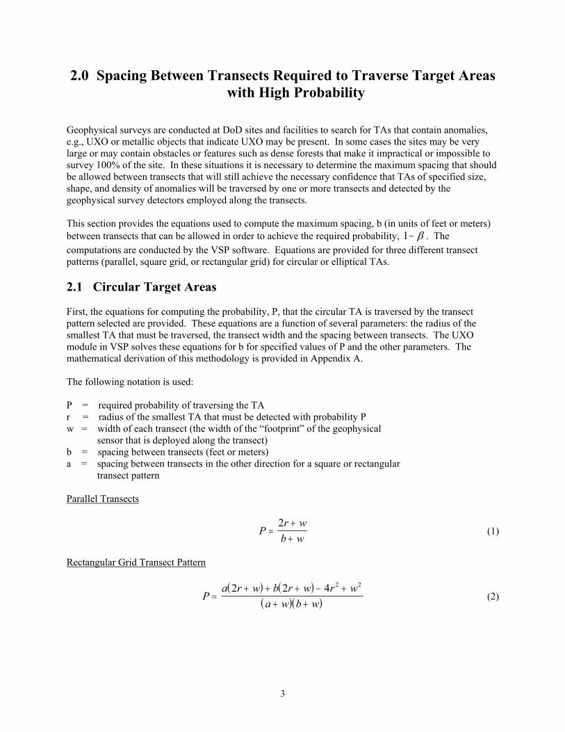
Geophysical surveys are conducted at DoD sites and facilities to search for TAs that contain anomalies, e.g., UXO or metallic objects that indicate UXO may be present. In some cases the sites may be very large or may contain obstacles or features such as dense forests that make it impractical or impossible to survey 100% of the site. In these situations it is necessary to determine the maximum spacing that should be allowed between transects that will still achieve the necessary confidence that TAs of specified size, shape, and density of anomalies will be traversed by one or more transects and detected by the geophysical survey detectors employed along the transects. This section provides the equations used to compute the maximum spacing, b (in units of feet or meters) between transects that can be allowed in order to achieve the required probability, 1− β . The computations are conducted by the VSP software. Equations are provided for three different transect patterns (parallel, square grid, or rectangular grid) for circular or elliptical TAs. 2.1 Circular Target Areas First, the equations for computing the probability, P, that the circular TA is traversed by the transect pattern selected are provided. These equations are a function of several parameters: the radius of the smallest TA that must be traversed, the transect width and the spacing between transects. The UXO module in VSP solves these equations for b for specified values of P and the other parameters. The mathematical derivation of this methodology is provided in Appendix A. The following notation is used: P = required probability of traversing the TA r = radius of the smallest TA that must be detected with probability P w = width of each transect (the width of the “footprint” of the geophysical sensor that is deployed along the transect) b = spacing between transects (feet or meters) a = spacing between transects in the other direction for a square or rectangular transect pattern Parallel Transects
Pr w
b w=
++
2 (1)
Rectangular Grid Transect Pattern
( ) ( )
( )( )Pa r w b r w r w
a w b w=
+ + + − ++ +
2 2 4 2 2
(2)
3

Square Grid Transect Pattern
( )
( )Pb r w r w
b w=
+ − ++
2 2 4 2 2
2 (3)
2.2 Elliptical Target Areas In addition to the notation given for circular targets in Section 2.1 above, the following additional notation is used: x = half-width of the TA rotated at an angle y = half-height of the TA rotated at an angle θ = angle of orientation of the TA with respect to the transect r1 = length of the semi-major axis of the TA r2 = length of the semi-minor axis of the TA Parallel Transects
P
y wb w
=+
+2
(4)
Rectangular Transect Pattern
( ) ( )
( )( )Pb x w a y w xy w
a w b w=
+ + + − ++ +
2 2 4 2
(5)
Square Transect Pattern
( ) ( )
( )Pb x w b y w xy w
b w=
+ + + − ++
2 2 4 2
2 (6)
where
x r d= −12 2 2sin θ
y r d= −12 2 2cos θ
d r r= −12
22
Known Angle of Orientation If the angle of orientation, θ , is known, the appropriate equation for P above (Equation 4, 5 or 6) is solved for b with a specified value of P and θ .
4
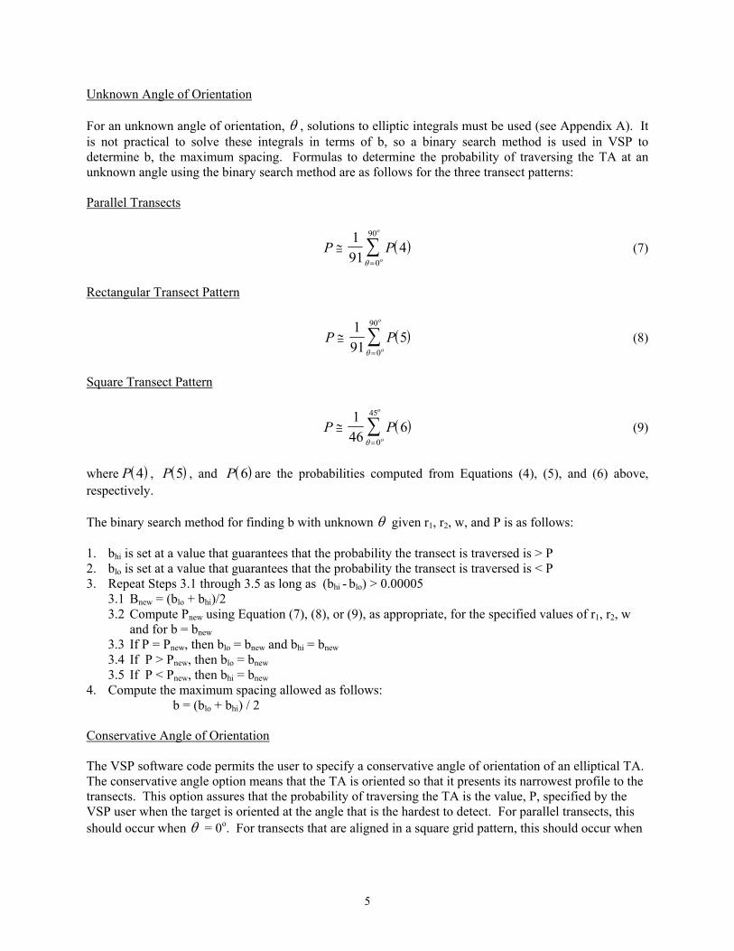
Unknown Angle of Orientation For an unknown angle of orientation, θ , solutions to elliptic integrals must be used (see Appendix A). It is not practical to solve these integrals in terms of b, so a binary search method is used in VSP to determine b, the maximum spacing. Formulas to determine the probability of traversing the TA at an unknown angle using the binary search method are as follows for the three transect patterns: Parallel Transects
( )P Po
o
≅=∑1
914
0
90
θ
(7)
Rectangular Transect Pattern
( )Po
o
≅=∑1
915
0
90
θ
P (8)
Square Transect Pattern
( )Po
o
≅=∑1
466
0
45
θ
P (9)
where , , and are the probabilities computed from Equations (4), (5), and (6) above, respectively.
( )P 4 ( )P 5 ( )P 6
The binary search method for finding b with unknown θ given r1, r2, w, and P is as follows: 1. bhi is set at a value that guarantees that the probability the transect is traversed is > P 2. blo is set at a value that guarantees that the probability the transect is traversed is < P 3. Repeat Steps 3.1 through 3.5 as long as (bhi - blo) > 0.00005 3.1 Bnew = (blo + bhi)/2 3.2 Compute Pnew using Equation (7), (8), or (9), as appropriate, for the specified values of r1, r2, w
and for b = bnew
3.3 If P = Pnew, then blo = bnew and bhi = bnew 3.4 If P > Pnew, then blo = bnew 3.5 If P < Pnew, then bhi = bnew 4. Compute the maximum spacing allowed as follows:
b = (blo + bhi) / 2 Conservative Angle of Orientation The VSP software code permits the user to specify a conservative angle of orientation of an elliptical TA. The conservative angle option means that the TA is oriented so that it presents its narrowest profile to the transects. This option assures that the probability of traversing the TA is the value, P, specified by the VSP user when the target is oriented at the angle that is the hardest to detect. For parallel transects, this should occur when θ = 0o. For transects that are aligned in a square grid pattern, this should occur when
5

θ = 45o. For transects that are in a rectangular grid pattern, this should occur when θ is between 0o and 45o, depending on the rectangle width-to-height ratio and the shape of the ellipse.
6

3.0 Probability of Traversing and Detecting a Target Area Section 2.0 presented the methods used to determine the maximum spacing between transects that will assure that a TA of specified size and shape will be traversed by one or more transects. However, the TA may not be detected even though it is traversed. The methods for computing the probability of both traversing and detecting a TA are documented in this section. The probability of traversing and detecting a TA of anomalies of a specified size, shape, and density is computed in VSP using the following formula: ( )PTD D T= −1 β P (10) where
1− β = probability that the TA is traversed by one or more transects
P = mean probability that the geophysical survey detects the TA given that the TA is traversed by one or more transects
D T
The VSP software code computes the probability PD T based on the value of VSP input parameters concerning the size and shape of the TA, the density of anomalies in the TA, and the false negative detection rate of the geophysical sensor system (as applied under normal field conditions) that will be used to conduct the surveys. The VSP user can specify that the model for the density (number per unit area) of anomalies is either a Uniform distribution (i.e., an unchanging mean density throughout the TA, i.e., the items are placed completely at random throughout the TA) or a Bivariate Normal distribution (the anomaly density is lowest at the edge of the TA and increases toward the center of the TA at a rate according to the Bivariate Normal distribution model). The VSP user must also specify both a critical density and a trigger density of anomalies. The critical density, (number/unit area), is the anomaly density in the TA that the stakeholders have determined must have a high probability of being detected by the geophysical survey so that the TA can be searched more closely for UXO. The trigger density ( ) is the lowest anomaly density of concern, that is, there is no need to find a TA that has an anomaly density that is less than the trigger density.
Dc
Dt
VSP computes PD T by (1) constructing a TA of the shape, size, and critical anomaly density specified by the VSP user, (2) placing that TA at a random location within the study site (e.g., suspected artillery impact range) such that all portions of the TA are within the boundary of the site, and by (3) specifying
, which is the false negative detection error rate (probability) of the geophysical sensor system under field operating conditions. In other words, it is assumed that each anomaly that lies within the portion of the TA that is traversed by one or more transects has the same probability, 1
Pfn
− Pfn , of being seen (detected) by the geophysical sensor system. The process VSP uses to compute the maximum spacing between transects is as follows:
1. The VSP user specifies
o the size (in mA 2, ft2, in2 or acres) and shape (circular or elliptical) of the TA of concern
7

o the probability, 1− β , required that the TA of that size and shape will be traversed by one or more transects
o whether a parallel, square grid, or rectangular grid transect design will be used o the width (the geophysical sensor “footprint”) of the transects (in units of meters, feet, or
inches) 2. VSP computes the maximum spacing between transects that will achieve the probability 1− β
that one or more transects will traverse the TA. A larger spacing will result in a probability less than 1− β of the TA being traversed.
3.1 Uniform Distribution Model for the Density of Anomalies in the Target
Area The process VSP uses to compute PD T is as follows if the VSP user has specified that the density of anomalies has the uniform distribution:
1. VSP places the TA at a random location within the study site such that the entire TA lies inside the study site
2. The VSP user specifies the critical and trigger densities ( and ) and the false negative detection error rate, , of the geophysical sensor system under field conditions. It is assumed that is the same value for each object that causes an anomalous reading.
Dc Dt
Pfn
Pfn
3. VSP computes the number of anomalies in the TA as follows: n ADTA c= 4. VSP uses simple random sampling to place the anomalies at random locations in the TA of
the specified size and shape nTA
5. VSP places the transect pattern at a random geographical starting place so that the transects cover the entire study site using the transect spacing, width, and pattern selected by the VSP user
6. VSP computes o the size of the area, , within the TA that is traversed by one or more of the transects
that happen to cross the TA, where 0 Att
Att ≥o the actual number of anomalies, , that lie within the area of size nd Att
o the number of anomalies, = , that are expected to lie within the area of size when the density of detectable items is at the trigger value,
ne Att Dt
Att Dt
7. VSP computes PD T , the probability the geophysical sensor has detected the TA given that the TA has been traversed by one or more transects, as follows:
( ) ( ) (Pn
i n iP PD T
d
dfn
i
fnn i
i n
nd
e
d
=−
− −
=∑ !
! !1 ) if n ≥ n (11) d e
PD T = 0 if n < n (12) d e
Then VSP repeats 10,000 times the process of placing the transect pattern at a random geographical starting place and recomputing , , andAtt nd ne PD T .
8. VSP computes the arithmetic mean, PD T , of the 10,000 values of PD T
9. Finally, VSP computes ( )P PTD D T= −1 β .
8
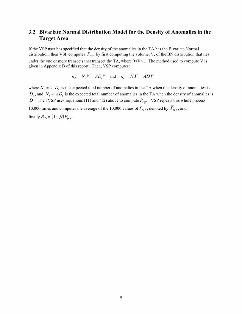
3.2 Bivariate Normal Distribution Model for the Density of Anomalies in the Target Area
If the VSP user has specified that the density of the anomalies in the TA has the Bivariate Normal distribution, then VSP computes PD T by first computing the volume, V, of the BN distribution that lies under the one or more transects that transect the TA, where 0<V<1. The method used to compute V is given in Appendix B of this report. Then, VSP computes:
n N V ADd c c= = V and n N V ADVe t t= = where is the expected total number of anomalies in the TA when the density of anomalies is
, and is the expected total number of anomalies in the TA when the density of anomalies is . Then VSP uses Equations (11) and (12) above to compute
N A Dc t=N At =
c
tDc
Dt
DPD T . VSP repeats this whole process
10,000 times and computes the average of the 10,000 values of PD T , denoted by PD T , and
finally ( )P PD TTD = −1 β .
9
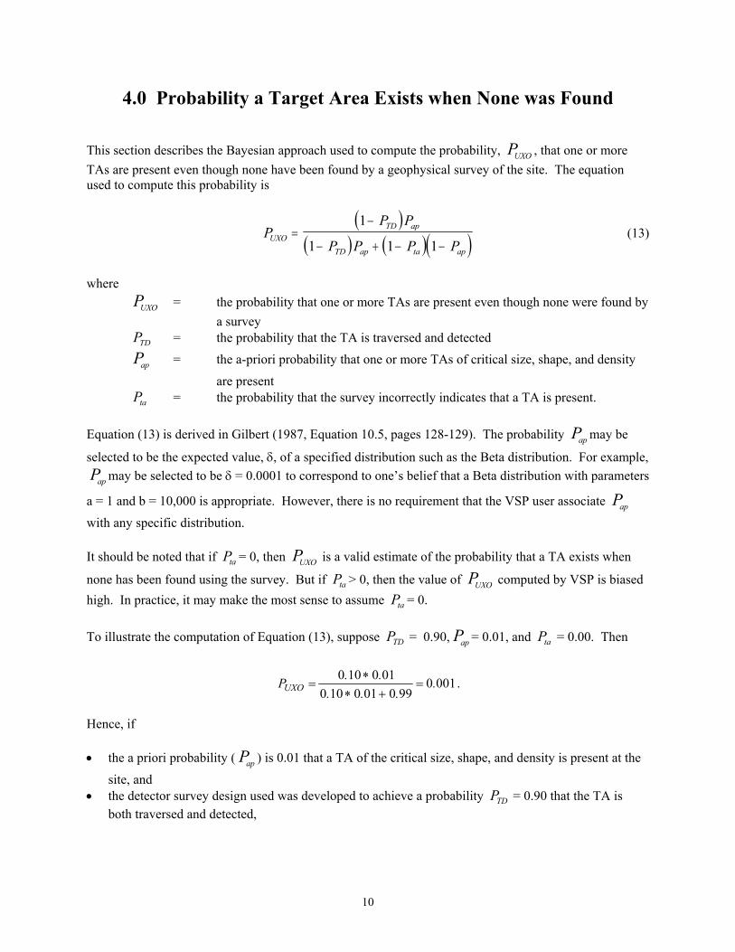
4.0 Probability a Target Area Exists when None was Found This section describes the Bayesian approach used to compute the probability, , that one or more TAs are present even though none have been found by a geophysical survey of the site. The equation used to compute this probability is
PUXO
( )
( ) ( )( )PP P
P P P PUXO
TD ap
TD ap ta ap
=−
− + − −
1
1 1 1 (13)
where
PUXO = the probability that one or more TAs are present even though none were found by a survey
PTD = the probability that the TA is traversed and detected Pap = the a-priori probability that one or more TAs of critical size, shape, and density
are present Pta = the probability that the survey incorrectly indicates that a TA is present.
Equation (13) is derived in Gilbert (1987, Equation 10.5, pages 128-129). The probability may be
selected to be the expected value, δ, of a specified distribution such as the Beta distribution. For example, may be selected to be δ = 0.0001 to correspond to one’s belief that a Beta distribution with parameters
a = 1 and b = 10,000 is appropriate. However, there is no requirement that the VSP user associate
with any specific distribution.
Pap
Pap
Pap
It should be noted that if = 0, then is a valid estimate of the probability that a TA exists when
none has been found using the survey. But if > 0, then the value of computed by VSP is biased high. In practice, it may make the most sense to assume = 0.
Pta PUXO
Pta PUXO
Pta
To illustrate the computation of Equation (13), suppose = 0.90, = 0.01, and = 0.00. Then PTD Pap Pta
0010990010100
010100 ....
..PUXO =+∗
∗= .
Hence, if • the a priori probability ( ) is 0.01 that a TA of the critical size, shape, and density is present at the
site, and
Pap
• the detector survey design used was developed to achieve a probability = 0.90 that the TA is both traversed and detected,
PTD
10

then the probability = 0.001 that a TA of the critical size, shape, and density exists either in the un-surveyed areas or in the surveyed areas even though the transect design used did not find any TAs.
PUXO
The verification that VSP is correctly computing Equation (13) is provided in Section 6.1.
11

5.0 Technical Basis of the Statistical Post-Survey Target Area Detection Evaluation Method
The transect sampling plans laid out by VSP are perfect straight lines that are spaced at regular intervals. However, when field crews implement a VSP sampling plan, they may find that obstacles, dense vegetation, geographic features and other factors make it undesirable, difficult, or impossible to follow straight lines with the geophysical sensors. This section documents the methods in VSP that can be used to approximate the probability that a TA of specified size and shape would have been found using the straight-line or meandering transects that were actually used in the geophysical survey. Section 5.1 documents the methods used in VSP to compute the probability of traversing meandering transects. Sections 5.2 and 5.3 document the methods used to compute the probability of both traversing and detecting the TA when the density of anomalies in the TA have a Uniform or Bivariate Normal distribution, respectively. 5.1 Approximating the Probability that Meandering Transects Traverse a
Target Area VSP defines transects as a series of connected points. Figure 5.1 depicts how connected points (and the line segments they define) may appear on a map.
Figure 5.1. Meandering Transects Depicted as a Series of Connected Points
In reality, transects have a width reflecting the width (“footprint”) of the geophysical sensor equipment as it traverses the ground. Hence, VSP represents the transects as a series of connected rectangles rather than as a series of connected line segments. VSP refers to these types of transects as meandering transects. Figure 5.2 depicts how meandering transects may appear.
12
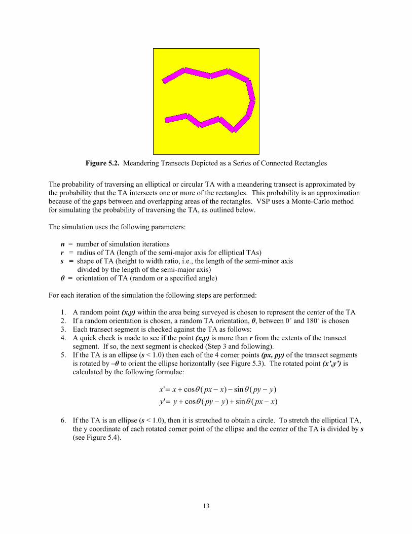
Figure 5.2. Meandering Transects Depicted as a Series of Connected Rectangles
The probability of traversing an elliptical or circular TA with a meandering transect is approximated by the probability that the TA intersects one or more of the rectangles. This probability is an approximation because of the gaps between and overlapping areas of the rectangles. VSP uses a Monte-Carlo method for simulating the probability of traversing the TA, as outlined below. The simulation uses the following parameters:
n = number of simulation iterations r = radius of TA (length of the semi-major axis for elliptical TAs) s = shape of TA (height to width ratio, i.e., the length of the semi-minor axis divided by the length of the semi-major axis) θ = orientation of TA (random or a specified angle)
For each iteration of the simulation the following steps are performed:
1. A random point (x,y) within the area being surveyed is chosen to represent the center of the TA 2. If a random orientation is chosen, a random TA orientation, θ, between 0˚ and 180˚ is chosen 3. Each transect segment is checked against the TA as follows: 4. A quick check is made to see if the point (x,y) is more than r from the extents of the transect
segment. If so, the next segment is checked (Step 3 and following). 5. If the TA is an ellipse (s < 1.0) then each of the 4 corner points (px, py) of the transect segments
is rotated by –θ to orient the ellipse horizontally (see Figure 5.3). The rotated point (x’,y’) is calculated by the following formulae:
)(sin)(cos')(sin)(cos'
xpxypyyyypyxpxxx
−+−+=−−−+=
θθθθ
6. If the TA is an ellipse (s < 1.0), then it is stretched to obtain a circle. To stretch the elliptical TA,
the y coordinate of each rotated corner point of the ellipse and the center of the TA is divided by s (see Figure 5.4).
13

Figure 5.3. Rotating the Elliptical Target Area to a Horizontal Orientation
Figure 5.4. Stretching the Elliptical Target Area to Make it a Circle
7. The rotated and stretched transect segment is checked against the circular TA to see if there is any overlap. If there is overlap, the hit count is increased by one and the next simulation iteration is tried (Step 1 and following). If there is no overlap, then the next transect segment is checked against the TA (Step 3 and following).
8. After all iterations have been tried, the probability of traversing the TA is given by the number of hits divided by n.
If the “Place samples on map to show simulation” option in VSP is selected, VSP places a point (black dot) on the site map for each trial TA location that was not traversed by the meandering transect. Figure
14
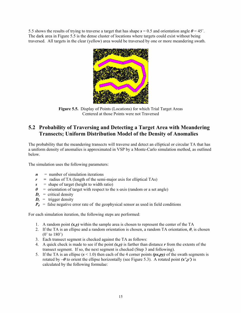
5.5 shows the results of trying to traverse a target that has shape s = 0.5 and orientation angle θ = 45˚. The dark area in Figure 5.5 is the dense cluster of locations where targets could exist without being traversed. All targets in the clear (yellow) area would be traversed by one or more meandering swath.
Figure 5.5. Display of Points (Locations) for which Trial Target Areas
Centered at those Points were not Traversed
5.2 Probability of Traversing and Detecting a Target Area with Meandering
Transects; Uniform Distribution Model of the Density of Anomalies The probability that the meandering transects will traverse and detect an elliptical or circular TA that has a uniform density of anomalies is approximated in VSP by a Monte-Carlo simulation method, as outlined below. The simulation uses the following parameters:
n = number of simulation iterations r = radius of TA (length of the semi-major axis for elliptical TAs) s = shape of target (height to width ratio) θ = orientation of target with respect to the x-axis (random or a set angle) Dc = critical density Dt = trigger density Pd = false negative error rate of the geophysical sensor as used in field conditions
For each simulation iteration, the following steps are performed:
1. A random point (x,y) within the sample area is chosen to represent the center of the TA 2. If the TA is an ellipse and a random orientation is chosen, a random TA orientation, θ, is chosen
(0˚ to 180˚) 3. Each transect segment is checked against the TA as follows: 4. A quick check is made to see if the point (x,y) is farther than distance r from the extents of the
transect segment. If so, the next segment is checked (Step 3 and following). 5. If the TA is an ellipse (s < 1.0) then each of the 4 corner points (px,py) of the swath segments is
rotated by –θ to orient the ellipse horizontally (see Figure 5.3). A rotated point (x’,y’) is calculated by the following formulae:
15

)(sin)(cos')(sin)(cos'
xpxypyyyypyxpxxx
−+−+=−−−+=
θθθθ
6. It is simpler to check the intersection of a circle than an ellipse, so if the target is an ellipse (s < 1.0) then the test plane is stretched vertically to make the target a circle. To stretch the plane, the y coordinate of each rotated corner point of the ellipse and the center of the target is divided by s (see Figure 5.4).
7. The rotated and stretched swath segment is checked against the TA circle to see if there is any overlap, as described in Appendix B (see separate documentation of the Polygon Intersect Circle Area algorithm in Section C1 of Appendix C). If there is no overlap, then the next transect segment is checked against the TA (Step 3 and following). If there is overlap, then the area of intersection between the transect segment and the TA is computed and added to the total intersection area (Att) (see separate documentation of the Polygon Intersect Circle Area algorithm in Section C1), the meandering swath segment is added to an array, and the next swath segment is checked against the target (Step 3 and following).
8. After all transect segments have been checked, overlapping transect segments in the array are found and any duplicated areas are removed from Att as outlined in Steps 9 through 11 below. There is a deficiency in this method of removal for multiple intersections as outlined in Section C10 of Appendix C.
9. Each transect segment in the array is checked against each other transect segment in the array. 10. If one transect segment in the array intersects another transect segment in the array, then the
intersection (the red and blue area in Figure 5.6) is turned into a polygon (see separate documentation for Polygon Intersecting Polygon algorithm in Section C2)
11. The intersection area between the intersection polygon and the target circle (the blue area in Figure 5.6) is found (see separate documentation of the Polygon Intersect Circle Area algorithm in Section C3) and subtracted from Att .
Figure 5.6. Finding the (Blue) Intersection Area between the Intersection Polygon and
the Target Area Circle
12. If Att is zero that indicates that no transect segments overlapped the TA. The Number of Misses
is increased by one and the next simulation iteration is tried (Step 1 and following). 13. At this point, Att is represented by the green and blue areas in Figure 5.6. If the target is an
ellipse, the test area must be squashed to turn the circle back into an ellipse so that Att represents the area in the original (un-stretched) test area. This transformation is accomplished by multiplying Att by s.
14. nd and ne are computed as follows:
16

ttte
cttd
DAnDAn
==
(note: nd and ne are rounded to the nearest integer) 15. If ne is zero, it is changed to one so that the following equation is correctly calculated 16. The probability that the sensor detects ne or more of the nd anomalies, PD T , is computed using
Equations 11 and 12 above 17. PD T is added to Total PD T . The PD T Count is increased by 1. The next simulation iteration is
tried (Step 1 and following). 18. When all n simulation iterations have been tried, the mean PD T is calculated as
PD T = (Total PD T ) / ( PD T Count) 19. The probability that the TA is traversed, 1-β, is calculated as
1-β = 1.0 – (Number of Misses) / n 20. The probability that the TA is traversed and detected, , is calculated as
= (1-β)
PTD
PTD PD T . If the “Place samples on map to show simulation” option is selected, VSP places a point where each trial target intersected one or more of the meandering swath segments. Figure 5.7 shows the results of trying to traverse a target of s = 0.5 and θ = 45˚. The clear (yellow) areas in Figure 5.7 are the locations where targets could exist without being traversed. All targets in the dark areas would be traversed by one or more meandering swath segments. More information can be found by right clicking on one of the samples that represents a simulated target. The sample label “56.5%,45” means 56.5% of the simulated target was traversed by meandering swath segments and the target was oriented at 45 degrees.
17

Figure 5.7. Dark Portions Indicate Areas that would be Traversed by One or More of the Meandering Transects for a Target Area of Shape s = 0.5 and θ = 45˚
5.3 Probability of Traversing and Detecting a Target Area with Meandering
Transects; Bivariate Normal Distribution Model of the Density of Anomalies
The probability of traversing and detecting an elliptical or circular target area with a meandering swath is approximated by a Monte-Carlo simulation method similar to the method used when the density of anomalies has a Uniform distribution (Section 4.2). The simulation uses the same parameters as are used for the Uniform distribution:
n = number of simulation iterations r = radius of TA (length of the semi-major axis for elliptical TAs) s = shape of target (height to width ratio) θ = orientation of target with respect to the x-axis (random or a set angle) Dc = critical density Dt = trigger density Pd = false negative error rate of the geophysical sensor
For each simulation iteration, the following steps are performed:
1. A random point (x,y) within the sample area is chosen to represent the center of the TA 2. If the TA is an ellipse and a random orientation is chosen, a random target orientation, θ, is
chosen (0˚ to 180˚) 3. Each transect segment is checked against the TA as follows: 4. A quick check is made to see if the point (x,y) is farther than distance r from the extents of the
swath segment. If so, the next segment is checked (Step 3 and following).
18
5. If the TA is an ellipse (s < 1.0), then each of the 4 corner points (px,py) of the swath segments is rotated by –θ to orient the ellipse horizontally (see Figure 5.3). A rotated point (x’,y’) is calculated by the following formulae:
)(sin)(cos')(sin)(cos'
xpxypyyyypyxpxxx
−+−+=−−−+=
θθθθ
6. It is simpler to check the intersection of a circle than an ellipse, so if the TA is an ellipse (s < 1.0)
then the test plane is stretched vertically to make the target a circle. To stretch the plane, the y coordinate of each rotated corner point of the ellipse and the center of the TA is divided by s (see Figure 5.4).
7. The rotated and stretched transect segment is checked against the TA circle to see if there is any overlap (see separate documentation of the Polygon Intersect Circle Area algorithm in Section C3 for details.) If there is no overlap, then the next transect segment is checked against the TA (Step 3 and following).
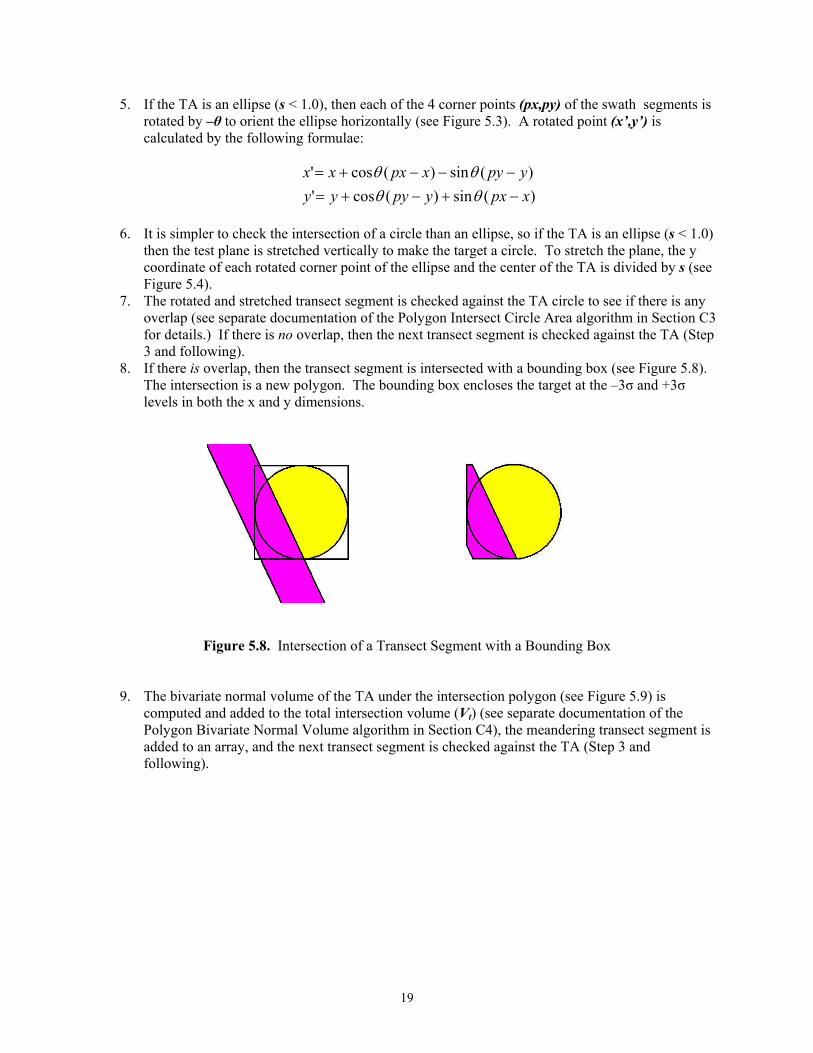
8. If there is overlap, then the transect segment is intersected with a bounding box (see Figure 5.8). The intersection is a new polygon. The bounding box encloses the target at the –3σ and +3σ levels in both the x and y dimensions.
Figure 5.8. Intersection of a Transect Segment with a Bounding Box
9. The bivariate normal volume of the TA under the intersection polygon (see Figure 5.9) is computed and added to the total intersection volume (Vt) (see separate documentation of the Polygon Bivariate Normal Volume algorithm in Section C4), the meandering transect segment is added to an array, and the next transect segment is checked against the TA (Step 3 and following).
19
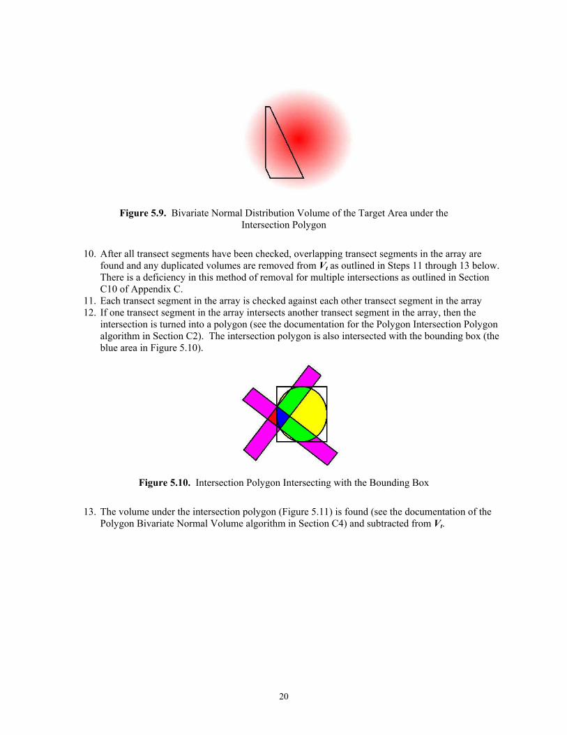
Figure 5.9. Bivariate Normal Distribution Volume of the Target Area under the
Intersection Polygon
10. After all transect segments have been checked, overlapping transect segments in the array are
found and any duplicated volumes are removed from Vt as outlined in Steps 11 through 13 below. There is a deficiency in this method of removal for multiple intersections as outlined in Section C10 of Appendix C.
11. Each transect segment in the array is checked against each other transect segment in the array 12. If one transect segment in the array intersects another transect segment in the array, then the
intersection is turned into a polygon (see the documentation for the Polygon Intersection Polygon algorithm in Section C2). The intersection polygon is also intersected with the bounding box (the blue area in Figure 5.10).
Figure 5.10. Intersection Polygon Intersecting with the Bounding Box
13. The volume under the intersection polygon (Figure 5.11) is found (see the documentation of the
Polygon Bivariate Normal Volume algorithm in Section C4) and subtracted from Vt.
20

Figure 5.11. Volume Under the Intersection Polygon
14. If Vt is zero, that means no transect segments overlapped the target area. The number of misses is
increased by one and the next simulation iteration is tried (Step 1 and following). 15. nd and ne are computed as follows:
ttte
cttd
DAVnDAVn
==
where: At = r2s is the area of the target ellipse and nd and ne are rounded to the nearest integer
16. If ne is zero, it is changed to one so that the following equation is correctly calculated. 17. The probability that the sensor detects ne or more of the nd detectable objects, PD T , is computed
using Equations 11 and 12 above 18. PD T is added to Total PD T . The PD T Count is increased by 1. The next simulation iteration is
tried (Step 1 and following). 19. When all n simulation iterations have been tried, the mean PD T is calculated as
PD T = (Total PD T ) / ( PD T Count) 20. The probability that the target is traversed, 1-β, is calculated as
1-β = 1.0 – (Number of Misses) / n 21. The probability that the TA is traversed and detected, , is calculated as PTD
PTD = (1-β) PD T . The “Place samples on map to show simulation” option in VSP works the same for the bivariate normal distribution as it does for the uniform distribution (see Figure 5.7 above). The sample label has a slightly different meaning: “56.5%, 45” means 56.5% of the volume of the simulated target was traversed by meandering swath segments and the target was oriented at 45 degrees.
21
6.0 Technical Basis of Compliance Sampling Methods This section describes the statistical methods selected by PNNL and used in VSP for determining the number of transects that should be surveyed and found to have no UXO to have high confidence that few if any UXO exist in transects that have not been surveyed. Such surveys may be necessary or desirable to support a no further action (NFA) decision for the area being surveyed. 6.1 Shilling’s Method for Determining the Number of Transects to Survey to
be Confident that Very Few Transects Contain UXO Suppose that in the area of interest there are N possible parallel transects that could be surveyed using a geophysical sensor, but that N is so large that only n transects can be surveyed, where n < N. How should n be determined? Shilling (1978, 1982) developed an acceptance sampling plan he called “compliance sampling” for determining n. He developed compliance sampling for industrial applications, but the methodology is also suitable for UXO applications and has been coded into VSP. For UXO applications, Shilling’s approach is implemented in VSP as follows:
• The VSP user specifies the width of each transect (all transects are assumed to have the same width)
• VSP uses the transect width and the map of the study area to compute the total number, N, of potential parallel transects that could be surveyed in the study area
• The VSP user specifies an upper limit on the percent, PL, of transects that contain one or more UXO that can be tolerated by the stakeholders. For example, the stakeholders may specify that no further action (or some other specified action) at the study site is needed if PL < 2 percent of the transects contain UXO
• The VSP user specifies the 100(1-ε) percent confidence, say 100(1 - 0.10) = 90%, that is required by the stakeholders that PL < 2 percent
• Then VSP computes the number, n, of the N transects that must be selected using simple random sampling and surveyed to find UXO
• If no UXO are found in the n transects and all transects are equal (or approximately equal) in length, then it can be stated that the probability is 0.90 that less than 2 percent of the N transects contain UXO.
As explained in Shilling [1978 and 1982 (pages 474-482)], n is determined by first computing D = N x PL and using D in a special table to find the fraction, f, of the N transects that must be surveyed. Then n = f x N. The fractions, f, in Shilling’s table are only appropriate when the required confidence is 90% (ε = 0.10). However, Shilling (1978, 1982) also shows how to determine the fraction, f, for any other confidence level that is desired.
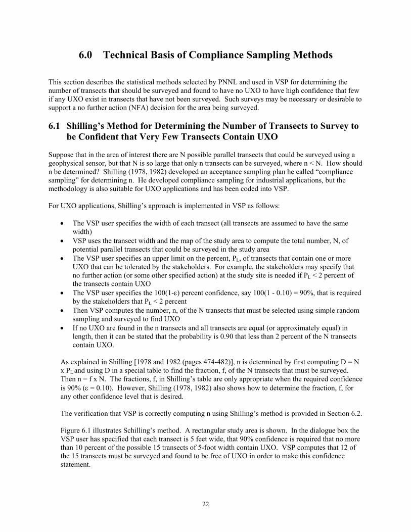
The verification that VSP is correctly computing n using Shilling’s method is provided in Section 6.2. Figure 6.1 illustrates Schilling’s method. A rectangular study area is shown. In the dialogue box the VSP user has specified that each transect is 5 feet wide, that 90% confidence is required that no more than 10 percent of the possible 15 transects of 5-foot width contain UXO. VSP computes that 12 of the 15 transects must be surveyed and found to be free of UXO in order to make this confidence statement.
22

Study Area
Dialogue Box
Figure 6.1. Illustration of Shilling’s Method in VSP for Determining the Number of Transects to be Surveyed to Assure Compliance with UXO Removal
Requirements 6.2 Wright and Grieve’s Method for Determining the Number of Transects
to Survey to be Confident that No Transects Not Surveyed Contain UXO Grieve (1994) developed an equation (his Equation 2.5) that can be used to compute the number of transects, n, that should be selected from the total set of N transects and found to contain no UXO in order to be 100(1-ε) percent confident that no UXO are present in the transects not surveyed. Grieve’s equation, which is based on the methods in Wright (1992), is coded into the VSP software. Wright and Grieve’s method is “Bayesian” because it requires that the stakeholders provide a quantitative measure of their belief that the study area contains UXO. This belief should be based on all information and data collected about the study area and the conceptual site model developed for the area. The stakeholders quantify their “belief” by choosing a specific Beta probability distribution for the fraction, f, of the N units that contain one or more UXO. [The Beta distribution is described in, e.g., Rothschild and Logothetis (1986, pages 50-51), Patel et al (1976) and Johnson and Kotz (1970).] In other words, the stakeholders are uncertain about the fraction of transects that contain UXO, but they can agree that the probability that f takes on various values can be modeled by a specific Beta distribution, the shape of which is determined by the value of the two parameters of the distribution: a and b. The expected (true average) value, δ , of f for a Beta distribution with parameter values a and b is δ = +a a b/ ( ) .
23

The VSP software allows the VSP user to choose among 7 possible Beta distributions. These distributions are listed in Table 6.1 and are illustrated in Figures 6.2 - 6.8. The shape of each distribution and the expected value δ for each distribution is determined by the values of the two parameters, a and b.
Table 6.1. The Seven Beta Distributions Available for Selection in VSP to Model the Uncertainty in the Fraction of Transects that Contain One or More UXO
Parameter Values of the Seven Beta Distributions
in VSP
Expected Value, δ,* of the Fraction, f, of Transects that
Contain UXO
English Characterization of the Beta Distribution used in
the VSP Software
1. a = 1, b = 999 0.001 Extremely low fraction 2. a = 1, b = 99 0.01 Very low fraction 3. a = 1, b = 9 0.1 Low fraction 4. a = 1, b = 1 0.5 All fractions equally
likely 5. a = 9, b = 1 0.9 High fraction 6. a = 99, b = 1 0.99 Very high fraction 7. a= 999, b = 1 0.999 Extremely high fraction
* δ = a/(a+b) The VSP user selects one of the seven distributions and VSP computes n using the following equation [derived from Equation 2.5 in Grieve (1994)]:
( ) ( )( ) ( ){ }n N N b b≥ − + − − −1 1 1ε δ δ/ (14) where N, a, b, δ and 1-ε have been defined above. If the geophysical sensor surveys do result in finding any UXO in any of the n randomly selected transects, then one can state with 100(1-ε) percent confidence that there are also no UXO in any of the N-n transects that were not surveyed. As is the case for Schilling’s method in Section 6.1, it is assumed that all transects are equal (or approximately) equal in length.
24
Beta Distribution (a=1, b=999)
f(p)
0
100
200
300
400
500
600
700
800
900
1000
Proportion of Units that contain UXO0.000 0.001 0.002 0.003 0.004 0.005 0.006
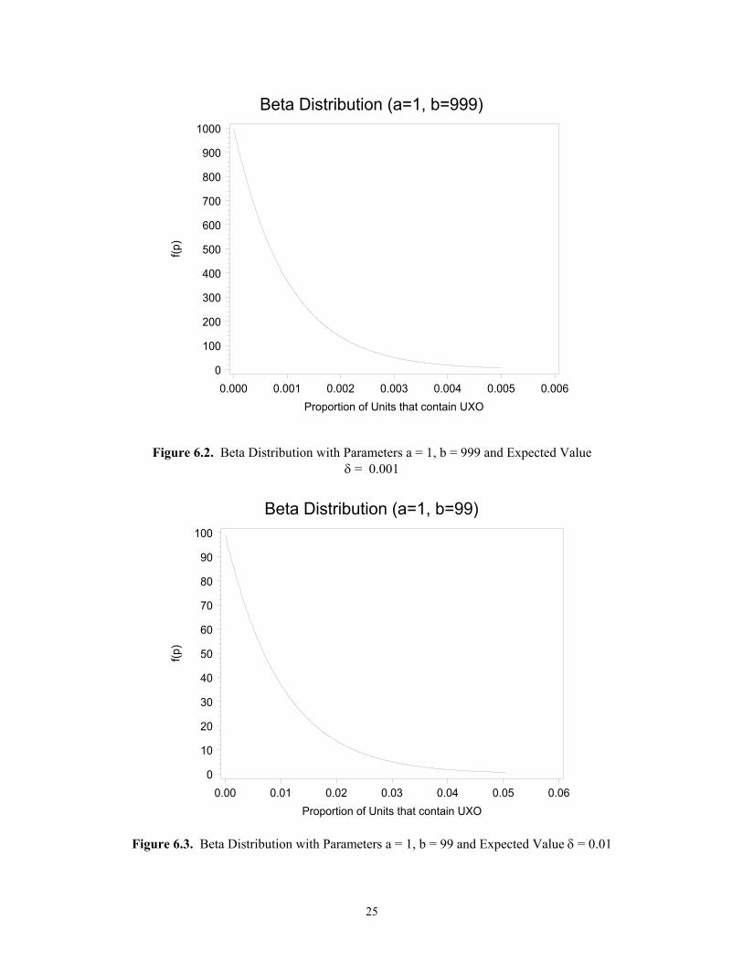
Figure 6.2. Beta Distribution with Parameters a = 1, b = 999 and Expected Value
δ = 0.001
Beta Distribution (a=1, b=99)
f(p)
0
10
20
30
40
50
60
70
80
90
100
Proportion of Units that contain UXO0.00 0.01 0.02 0.03 0.04 0.05 0.06
Figure 6.3. Beta Distribution with Parameters a = 1, b = 99 and Expected Value δ = 0.01
25

Beta Distribution (a=1, b=9)
f(p)
0
1
2
3
4
5
6
7
8
9
Proportion of Units that contain UXO0.0 0.1 0.2 0.3 0.4 0.5 0.6
Figure 6.4. Beta Distribution with Parameters a = 1, b = 9 and Expected Value δ = 0.1
Beta Distribution (a=1, b=1)
f(p)
1
Proportion of Units that contain UXO0.0 0.1 0.2 0.3 0.4 0.5 0.6 0.7 0.8 0.9 1.0
Figure 6.5. Beta Distribution with Parameters a = 1, b = 1 and Expected Value δ = 0.5
26
Beta Distribution (a=9, b=1)
f(p)
0
1
2
3
4
5
6
7
8
9
Proportion of Units that contain UXO0.60 0.65 0.70 0.75 0.80 0.85 0.90 0.95 1.00
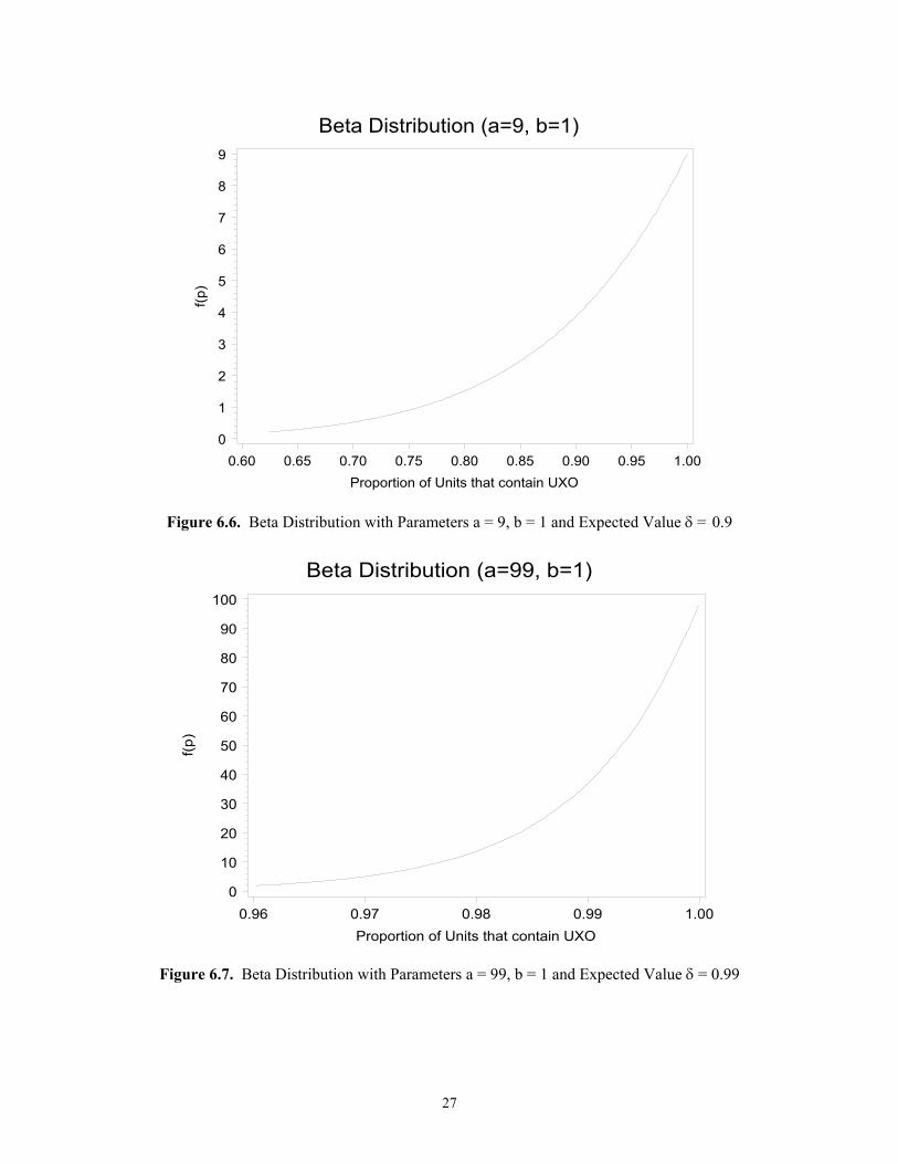
Figure 6.6. Beta Distribution with Parameters a = 9, b = 1 and Expected Value δ = 0.9
Beta Distribution (a=99, b=1)
f(p)
0
10
20
30
40
50
60
70
80
90
100
Proportion of Units that contain UXO0.96 0.97 0.98 0.99 1.00
Figure 6.7. Beta Distribution with Parameters a = 99, b = 1 and Expected Value δ = 0.99
27

Beta Distribution (a=999, b=1)
f(p)
0
100
200
300
400
500
600
700
800
900
1000
Proportion of Units that contain UXO0.996 0.997 0.998 0.999 1.000
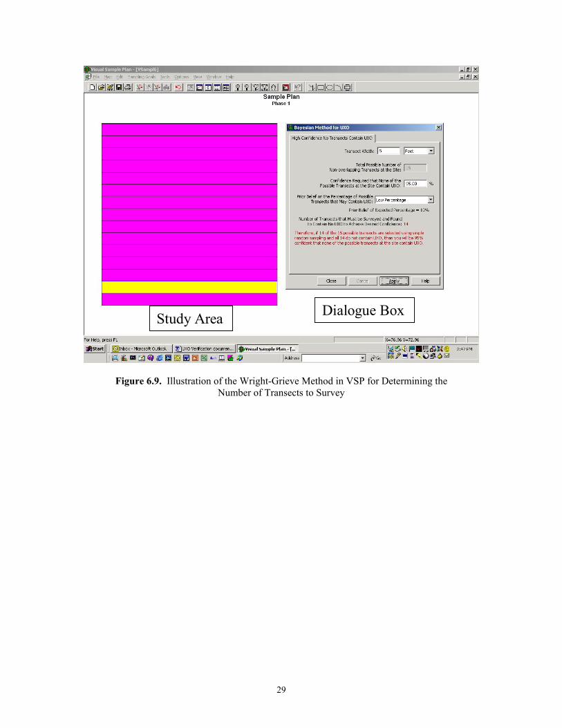
Figure 6.8. Beta Distribution with Parameters a = 999, b = 1 and Expected Value δ = 0.999 Figure 6.9 illustrates the Wright-Grieve method. A rectangular study area is shown. In the dialogue box the VSP user has specified that each transect is 5 feet wide, that it is the VSP user’s prior belief that 10% of the transects in the study area may contain UXO and that 95% confidence is required that there are no UXO in the study area if no UXO are found in the n transects that are surveyed. With these specifications, VSP computes that 14 of the 15 transects must be surveyed and found to have no UXO in order to have 95% confidence that no UXO are present in the study area.
28
Study Area Dialogue Box
Figure 6.9. Illustration of the Wright-Grieve Method in VSP for Determining the Number of Transects to Survey
29

7.0 Verification of Visual Sample Plan Software UXO Module Computations
This section documents the hand or computer calculations conducted at PNNL to verify that VSP is correctly computing
• the probability that a TA exists when none has been found (Section 7.1) • the number of transects, n, as determined using Shilling’s method (Section 7.2) • the number of transects, n, as determined using the Wright and Grieve method (Section 7.3), and • the number of anomalies that occur in the portion of the transects that traverse the TA when the
density of the anomalies in the TA has a Bivariate Normal Distribution (Section 7.4). 7.1 Probability a Target Area Exists when None was Found This section documents the agreement between hand and VSP calculations of the probability, , that a TA exists when none were found during the geophysical survey of the study area. VSP used Equation (13) in Section 4.0 to compute this probability. The calculation results are presented in Table 7.1. There was perfect agreement of the hand and VSP calculation of for the six combinations of Equation (13) parameters used in Table 7.1.
PUXO
PUXO
Table 7.1. Values of the Probability that a Target Area Exists when None was Found by
a Geophysical Survey
PTP Pap Pta PUXO Computed by
Hand
PUXO Computed b
VSP 0.50 0.50 0.50 0.50 0.50 0.90 0.50 0.50 0.16667 0.16667 0.90 0.10 0.50 0.02174 0.02174 0.90 0.10 0.05 0.01156 0.01156 0.999 0.0001 0.01 0.000 0.000 0.001 0.999 0.001 0.999 0.999 0.90 0.999 0.000 0.990 0.990
7.2 Shilling’s Method for Computing the Number of Transects to Survey The test results are provided in Table 7.2. We see that there is perfect agreement between the VSP and hand calculations of n, the number of transects that need to be selected using simple random sampling, surveyed, and found to contain no UXO in order to state with specified confidence that the percentage of the total number of possible transects that contain one or more UXO is less than the specified value PL.
30

Table 7.2. Comparison of Values of n Computed using VSP and by Hand
N* PL **
Confidence Required
n Computed by Hand
n Computed using VAP
10 1 % 90 % 10 10 10 0.769 % 95 % 10 10 100 0.769 % 95 % 95 95 100 1 % 90% 90 90 100 10 % 90 % 21 21 100 2 % 99 % 90 90 1000 0.769 % 95 % 259 259 1000 5 % 90 % 46 46 1000 10 % 90 % 206 206 10000 0.769 % 95 % 297 297 10000 1 % 90 % 237 237
* Number of potential transects in the study area ** Upper limit on the percent, PL, of transects that contain one or more UXO that can be tolerated by the stakeholders.
7.3 Wright and Grieve’s Method for Computing the Number of Transects to
Survey The test results are presented in Tables 7.3, 7.4, 7.5, and 7.6 for N = 10, 100, 1000 and 10,000, respectively. Recall from Section 6.2 that N is the total number of potential transects in the study area. In all cases, the hand calculation of n agreed with the VSP calculation of n after the hand calculations were rounded up to the next largest integer. Both the hand and VSP calculations were made using Equation 14. Because perfect agreement in n was obtained (after rounding up) in all cases, the table entries are the values of n obtained by VSP. Recall that δ is the expected fraction of the N transects that contain UXO. Each value of δ corresponds to a different Beta distribution (see Table 6.1 and Figures 6.2 through 6.8). These tables provide information on how n changes with changes in the confidence required, the Beta distribution, and the number of potential transects, N. Clearly, the number of transects, n, that need to be surveyed and found to not contain UXO increases greatly as the required confidence increases, as the expected fraction of transects that contain UXO increase, and as N increases. Also, it should be noted in Table 7.3 and 7.4 that a value of n = 0 indicates the actual n computed by hand and by VSP using Equation 14 was negative. VSP converts these negative values to zero because a negative n has no meaning.
31
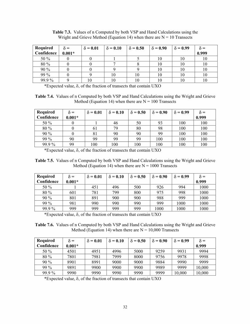
Table 7.3. Values of n Computed by both VSP and Hand Calculations using the Wright and Grieve Method (Equation 14) when there are N = 10 Transects
Required Confidence
δ = 0.001*
δ = 0.01 δ = 0.10 δ = 0.50 δ = 0.90 δ = 0.99 δ = 0.999
50 % 0 0 1 5 10 10 10 80 % 0 0 7 8 10 10 10 90 % 0 0 9 9 10 10 10 99 % 0 9 10 10 10 10 10 99.9 % 9 10 10 10 10 10 10
*Expected value, δ, of the fraction of transects that contain UXO
Table 7.4. Values of n Computed by both VSP and Hand Calculations using the Wright and Grieve Method (Equation 14) when there are N = 100 Transects
Required Confidence
δ = 0.001*
δ = 0.01 δ = 0.10 δ = 0.50 δ = 0.90 δ = 0.99 δ = 0.999
50 % 0 1 46 50 93 100 100 80 % 0 61 79 80 98 100 100 90 % 0 81 90 90 99 100 100 99 % 90 99 99 99 100 100 100 99.9 % 99 100 100 100 100 100 100
*Expected value, δ, of the fraction of transects that contain UXO
Table 7.5. Values of n Computed by both VSP and Hand Calculations using the Wright and Grieve Method (Equation 14) when there are N = 1000 Transects
Required Confidence
δ = 0.001*
δ = 0.01 δ = 0.10 δ = 0.50 δ = 0.90 δ = 0.99 δ = 0.999
50 % 1 451 496 500 926 994 1000 80 % 601 781 799 800 975 998 1000 90 % 801 891 900 900 988 999 1000 99 % 981 990 990 990 999 1000 1000 99.9 % 999 999 999 999 1000 1000 1000
*Expected value, δ, of the fraction of transects that contain UXO
Table 7.6. Values of n Computed by both VSP and Hand Calculations using the Wright and Grieve Method (Equation 14) when there are N = 10,000 Transects
Required Confidence
δ = 0.001*
δ = 0.01 δ = 0.10 δ = 0.50 δ = 0.90 δ = 0.99 δ = 0.999
50 % 4501 4951 4996 5000 9259 9931 9994 80 % 7801 7981 7999 8000 9756 9978 9998 90 % 8901 8991 9000 9000 9884 9990 9999 99 % 9891 9900 9900 9900 9989 9999 10,000 99.9 % 9990 9990 9990 9990 9999 10,000 10,000
*Expected value, δ, of the fraction of transects that contain UXO
32

7.4 Computing the Number of Anomalies when the Density of Anomalies in the Target Area has a Bivariate Normal Distribution
As discussed in Sections 3.1 and 3.2, in order to compute the probability of traversing and detecting a TA, it is necessary to first compute, , which is the number of anomalies that are present within that portion of the transects that cross over the TA. If the density of anomalies within the TA has a Uniform distribution (i.e., anomalies occur at random locations throughout the TA at a specified density), then
is easily determined. But if the density has a Bivariate Normal distribution, the computation of is much more complex, as is detailed in Appendix B. Hence, it is important to verify that VSP is correctly computing using the method in Appendix B.
nd
nd nd
nd
VSP uses the C++ computer language to compute . The accuracy of the computations was assessed by independent computation of n by a second individual in the Statistical and Quantitative Sciences Group, Mr. Robert F. O’Brien, using a different computer language (from Mathematica software). Table 7.7 provides the testing results.
nd
d
The notation in Table 7.7 is defined as follows:
b = spacing between transects a = spacing between transects in the other direction w = width of each transect r1 = length of semi-major axis of the elliptical TA r2 = length of semi-minor axis of the elliptical TA D = density of anomalies in the TA nTA = number of anomalies in the TA nd = the average number of anomalies that are present within that portion of the transects that cross over the TA (based on 10,000 simulations)
% Difference = % difference in the two computed value of n d
The last column indicates that for the 12 cases considered, the value of n computed by VSP deviated from the value of
d
nd computed by Mr. O’Brien using Mathematica code by no more than 1.9%.
Table 7.7. Values of nd Computed by VSP Versus that Computed Using Mathematica Computer Code
Case
b
a
w
r1
r2
D
nTA
nd
(VSP)
nd
(O’Brien)
% Differ-ence in nd
1 10 10 5 5 5 300 23562 13018 13045 0.21 2 8 16 4 5 4 300 18850 8855 8804 0.58 3 5 15 3 5 2.5 300 11781 5679 5679 0.00 4 35 70 5 5 5 300 23562 4290 4290 1.9 5 15.570 23.36 3 5 3.75 300 17671 4571 4491 1.8 6 16.729 16.73 3 5 2.5 300 11781 3288 3338 1.5 7 13.25 * 3 5 5 300 23562 4272 4348 -1.8 8 10.384 * 3 5 2.5 300 11781 2636 2631 0.2
33

Table 7.7. Values of nd Computed by VSP Versus that Computed Using Mathematica Computer Code (cont.)
Case
b
a
w
r1
r2
D
nTA
nd
(VSP)
nd
(O’Brien)
% Differ-ence in nd
9** 7 * 3 5 2.5 300 11781 3508 3525 -0.5 10*** 13.25 * 3 5 2.5 300 11781 2156 2175 -0.8 11** 12.661 18.99 3 5 2.5 300 11781 3526 3556 -0.8 12*** 22.934 15.29 3 5 2.5 300 11781 3047 3071 -0.8
* Parallel transects rather than perpendicular transects were used ** The TA was orientated at a fixed angle = 0 degrees relative to the x axis *** The TA was orientated at a fixed angle = 90 degrees relative to the x axis
For Cases 9, 10, 11, and 12, the value of n (O’Brien) (10d
th column) was computed using numerical integration of the expected value, rather than using 10,000 simulations.
34
8.0 References Gilbert, R.O. 1987. Statistical Methods for Environmental Pollution Monitoring, Wiley & Sons, New York, NY Gilbert, R.O., B.A. Pulsipher, D.K. Carlson, R.F. O’Brien, J.E. Wilson, D.J. Bates, and. G.A. Sandness. 2001. Designing UXO Sensor Surveys for Decision Making, Pacific Northwest National Laboratory, Richland, WA Grieve, A.P. 1994. “A Further Note on Sampling to Locate Rare Defectives with Strong Prior Evidence,” Biometrika 81(4):787-789. Hassig, N.L., J.E. Wilson, R.O. Gilbert, D.K. Carlson, R.F. O’Brien, B.A. Pulsipher, C.A. McKinstry, and D.J. Bates, 2002. Visual Sample Plan Version 2.0 User’s Guide, PNNL-14002, Pacific Northwest National Laboratory, Richland, WA. Johnson, N.L. and S. Kotz. 1970. Continuous Univariate Distributions-2, Houghton Mifflin Company, Boston, MA. Patil, J.K., C.H. Kapadia and D.B. Owen. 1976. Handbook of Statistical Distributions, Marcel Dekker, Inc., New York, NY. Rothschild, V. and N. Logothetis. 1986. Probability Distributions, John Wiley & Sons, New York, NY. Shilling, E.G. 1978. “A Lot Sensitive Sampling Plan for Compliance Testing and Acceptance Inspection,” Journal of Quality Technology 10(2):47-51. Shilling, E.G. 1982. Acceptance Sampling in Quality Control, Marcel Dekker, Inc, New York, NY. Wright, T. 1992. “A Note on Sampling to Locate Rare Defectives with Strong Prior Evidence,” Biometrika 79(4):685-691.
35

APPENDIX A
Probabilities that a Rectangular Grid of Transects of Specified Width Will Intersect an Elliptical Target Area

A.1
APPENDIX A
Probabilities that a Rectangular Grid of Transects of Specified Width Will Intersect an Elliptical Target Area
Robert F. O’Brien
Statistical and Quantitative Sciences Pacific Northwest National Laboratory
Richland, Washington 99352
1.0 Introduction A problem often considered in environmental characterization and remediation is to develop a sampling scheme for traversing a contaminated target area of a specified size and shape. The typical approach is to define a systematic grid pattern of sampling points that will have a specified probability of traversing a randomly located target area of concern. When the sampling points lie on the nodes of a rectangular or triangular grid of field transects and the specified target area is elliptical, Gilbert (1987) discusses a method developed by Singer (1972, 1975) that gives the proper grid spacing for the nodes. When the grid is rectangular and the sampling points are continuous along the transects, Duma and Stoka (1993) give a methodology to find the probability of traversing a randomly located elliptical target for the special case when both axes of the ellipse are less than the length of the smallest side of an elementary rectangle of the grid. This paper extends the results of Duma and Stoka’s methodology to the more general case where the transects may also have a specified width and further includes the case where one of the axes of the ellipse may be shorter than one of the sides of an elementary rectangle of the grid. This paper develops a methodology of finding the probability of the grid traversing an elliptical target of a specified size when a rectangular grid is used for sampling and the transects have a specified width. This probability can then be used to determine the spacing between the transects of the grid that is necessary to traverse a specified elliptical target with a specified probability. This methodology was developed for the situation in which a nondestructive assay device such as a magnetometer or ground penetrating radar is used to pass over the transects of a rectangular grid looking for elliptically shaped clusters of shrapnel that may indicate the existence of unexploded ordnance (UXO). In these situations, the field of view of the magnetometer or ground penetrating radar has a given width. The methodology, however, is applicable to any environmental situation where a measurement device collects continuous, or near continuous, measurements of a certain width along a transect.

A.2
2.0 Methodology To find the dimensions of the grid (distance between transects) it is sufficient to develop a relationship that gives the probability of the grid traversing an elliptical target area as a function of the parameters that define an elementary rectangle of the grid and the ellipse. This follows from the fact that if the grid traverses the target ellipse then the ellipse’s center must lie in one of the elementary rectangles of the grid. Once a formula for this probability is developed, it is only a matter of solving for the unknown parameters of the elementary rectangle of the grid to find the appropriate grid spacing needed to find an ellipse of a specified size with a given probability. Section 2.1 develops a formula for the probability of a randomly placed target ellipse intersecting an elementary rectangle of the grid in terms of the parameters that define an elementary rectangle of the grid and the ellipse. Two cases are considered; one where the dimensions of the ellipse are such there exists a set of points inside an elementary rectangle of the grid where the ellipse can be fully rotated 360 degrees about its center without intersecting the grid, the other case is where there is no such set of points where the ellipse can be fully rotated 360 degrees about its center without intersecting the ellipse. Section 2.2 discusses certain special cases for the parameters of the grid and target ellipse. These special cases are: 1) where the grid consists of only parallel transects, 2) where the target area is a circle, 3) when the angle of orientation to the grid is known, and 4) when there may be more than one target ellipse. Section 3 gives examples using these formulas to find grid dimensions that will yield a specified probability of traversing the target ellipse when the target ellipse and transect widths are specified. 2.1 Probability of an Ellipse Intersecting an Elementary Rectangle of the
Grid Let L be a rectangular grid in the Euclidean plane whose transects have a specific width w1 in the north-south direction and w2 in the east-west direction. Without loss of generality, let an elementary rectangle of this grid, T(a+w1, b+w2 ), be defined as
T (a + w1,b + w2 ) = Bii=1
4U
where
}. ,0|),{(
},0 ,|),{(
},0 ,0|),{(
},0 ,0|),{(
214
13
2
1
wbybwaxyxB
bywaxayxB
byxyxB
yaxyxB
+<≤+<<=<≤+<≤=
<<===<≤=
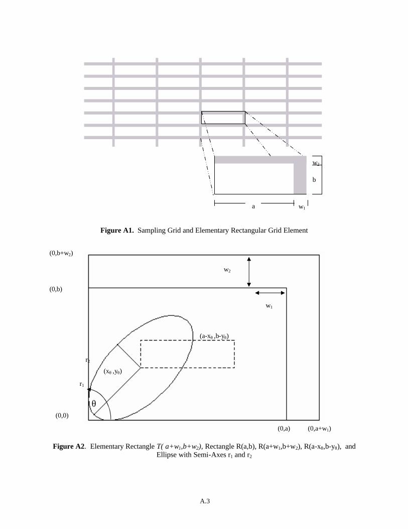
Also define R(a+w1, b+w2 ) as the rectangle formed by the vertices (0,0), ( a+w1 ,0), (a+w1, b+w2 ) and (0, b+w2 ). Similarly define R(a,b). We are interested in finding the probability of an ellipse with semi- axes r1 and r2 , r2 ≤ r1, whose center lies inside the rectangle R(a+w1, b+w2 ) that intersects an elementary rectangle T(a+w1, b+w2 ) of the grid. This probability, P, assumes that the center of the ellipse and its angle θ between its main axis and the side a+w1 are independent uniformly distributed on T(a+w1, b+w2 ) and on [0,π) respectively. Figures A1 and A2 show a graphic of the grid and T(a+w1, b+w2 ), R(a+w1, b+w2 ), R(a,b) and an ellipse.
A.3
Figure A1. Sampling Grid and Elementary Rectangular Grid Element
Figure A2. Elementary Rectangle T( a+w1,b+w2), Rectangle R(a,b), R(a+w1,b+w2), R(a-xθ,b-yθ), and Ellipse with Semi-Axes r1 and r2
w2
w1
(xθ ,yθ)
(a-xθ ,b-yθ)
(0,0)
(0,a) (0,a+w1)
(0,b)
(0,b+w2)
θ
r1
r2
b
w2
a w1

A.4
For a given angle θ, an ellipse with center at (xθ,yθ) will lie just inside the rectangle R(a,b) without intersecting R(a,b) when xθ = (r1
2 − d2 sin2 θ)1/ 2and yθ = (r12 − d2 cos2 θ)1/ 2 , where d2 = r1
2 – r22. This
can be shown using differential calculus, noting that -xθ and xθ, are the minimum and maximum x values of the ellipse with respect to y and -yθ and yθ, are the minimum and maximum y values of the ellipse with respect to x when the ellipse has center at the origin and whose major axis is at an angle θ to the x–axis. To find the probability, P, it is sufficient to only find the probability, Q, that the ellipse does not intersect R(a,b), since
P =1−ab
(a + w1)(b + w 2)Q .
There are two cases to consider: one where 2r2 ≤ 2r1 < min{a,b} and the other when 2r2 < min{a,b} ≤ 2r1 < max{a,b}. In the first case, if the ellipse has its center in the rectangle R(a- xθ,, b- yθ,) formed by the vertices (xθ,yθ), (a-xθ,yθ), (a-xθ,b-yθ), and (xθ,b-yθ) the ellipse never intersects R(a,b) for all angles θ, where 0< θ < π.. In the second case this is not true for all 0< θ < π. Case 1: 2r2 = 2r1 < min{a,b} To find Q in this case note that an ellipse with semi-axes r1 and r2 and angle θ will not intersect R(a,b) if the center lies in the rectangle R(a- xθ, b- yθ,). In this case Duma and Stoka show that the probability of the ellipse not intersecting the rectangle R(a,b) is given by
Q = πab( )−1 (a −2xθ )(b −2yθ )dθ0
π∫= πab( )−1 [a − 2 r1
2 − d2 sin2 θ( )1/ 2][b − 2 r1
2 − d2 cos2 θ( )1/ 2]dθ
0
π∫= πab( )−1[4(a + b)r1E( d 2
r12 ) − 8 r1r2( )E − d 4
4r12r2
2 )( )]
where E(•) is a complete elliptic integral of the second kind defined as E(z) = 1− zsin2 (ϕ)0
π / 2∫ dϕ . It
then follows that
P =1− ab(a + w1)(b + w 2)
Q
=1−a − 2 r1
2 − d2 sin 2 θ( )1/ 2[ ]b − 2 r12 − d2 cos2 θ( )1/ 2[ ]dθ
0
π∫π (a + w1)(b + w2 ) .
Here numerical integration is required to obtain the desired probability. This is easiest to implement using Gaussian quadrature. Case 2: 2r2 < min{a,b} = 2r1 < max{a,b} In this case for a given angle θ, the ellipse will not intersect R(a,b) only if the center of the ellipse is in the
rectangle R(a- xθ,, b- yθ,) where 0 <θ < cos-1 (r12 − b2 / 4) /d2( ) or
A.5
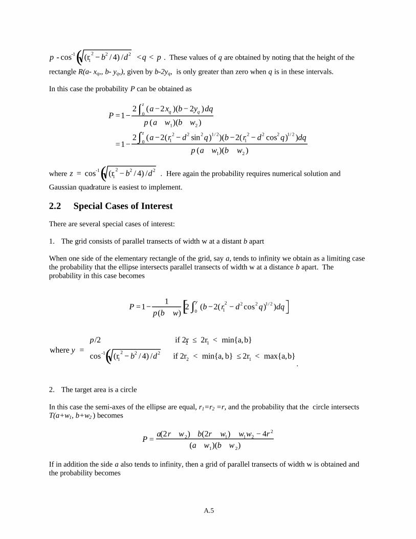
π - cos-1 (r12 − b2 / 4) /d2( )<θ < π . These values of θ are obtained by noting that the height of the
rectangle R(a- xθ,, b- yθ,), given by b-2yθ, is only greater than zero when θ is in these intervals. In this case the probability P can be obtained as
P =1−2 (a −2xθ )(b − 2yθ )dθ
0
ζ∫π (a + w1)(b + w2 )
=1−2 (a −2(r1
2 − d2 sin2 θ)1/ 2)(b −2(r12 − d2 cos2 θ)1/ 2 )dθ
0
ζ∫π (a + w1)(b + w2 )
where ζ = cos-1 (r12 − b2 / 4) /d2( ). Here again the probability requires numerical solution and
Gaussian quadrature is easiest to implement. 2.2 Special Cases of Interest There are several special cases of interest: 1. The grid consists of parallel transects of width w at a distant b apart When one side of the elementary rectangle of the grid, say a, tends to infinity we obtain as a limiting case the probability that the ellipse intersects parallel transects of width w at a distance b apart. The probability in this case becomes
P =1−1
π(b + w)2 (b −2(r1
2 − d2 cos2 θ)1/ 2 )dθ0
ψ∫[ ]
where ψ =π/2 if 2r2 ≤ 2r1 < min{a,b}
cos -1 (r12 − b2 / 4) /d2( ) if 2r2 < min{a, b} ≤ 2r1 < max{a,b}
.
2. The target area is a circle In this case the semi-axes of the ellipse are equal, r1=r2 =r, and the probability that the circle intersects T(a+w1, b+w2 ) becomes
P =a(2r + w2) + b(2r + w1) + w1w2 − 4r 2
(a + w1)(b + w 2)
If in addition the side a also tends to infinity, then a grid of parallel transects of width w is obtained and the probability becomes

A.6
P =2r +w 2
b + w 2 .
3. The angle of orientation, θ, is known If the angle of orientation of the ellipse to the grid is already known, θ, then the probability of the ellipse not intersecting R(a,b), Q, becomes
(Area of R(a- xθ,, b- yθ,)) /(Area of R(a, b))
and the probability , P, becomes
P =1−(a − 2(r1
2 − d2 sin2 θ)1/ 2)(b − 2(r12 − d 2 cos2 θ)1/ 2 )
(a + w2 )(b + w1)
where θ is an element of (0, 2π) if 2r2 = 2r1 < min{a,b}, or θ is an element of one of the intervals
[0, cos-1 (r12 −b 2 /4)/ d 2( )] or [π - cos-1 (r1
2 −b2 /4) /d2( ), π ] if 2r2 < min{a,b} = 2r1 < max{a,b}.
4. The probability of intersecting more than one ellipse The probability of one ellipse intersecting the grid is given above as P. If there is interest in there possibly being more than one ellipse of interest in the Euclidean plane then the probability of intersecting at least one of n possible ellipses of the same size can be obtained as follows: For a given ellipse and a given grid the probability of intersecting one ellipse that is randomly placed on the Euclidean plane is given by P above. If there are n ellipses of interest, all of the same size and independently distributed on the Euclidean plane, then the probability of not intersecting any of the ellipses with the given grid is 1− P( )n
. Thus, the probability of intersecting at least one ellipse is given
by 1− (1− P)n . If each of the n ellipses is of a different size and independently distributed on the Euclidean plane, then each ellipse has a probability of Pi of intersecting the grid where Pi depends on the length of the semi-axes of each ellipse. Then the probability of the grid not intersecting any of the ellipses is given by
1− Pi( )i=1
n∏ and thus the probability of the grid intersecting at least one of the ellipses is given by
1− 1− Pi( )i=1
n∏ .
It should be noted that the probabilities above were mostly solved when the transect widths may be different, w1 ? w2, to cover the most general case. This was done to cover the instances where parallel transects, say north-south, may be done at one time using some non-destructive instrument or array of instruments and the east-west transects were done at another time possibly using a different non-destructive device or array of devices. In most real applications w1=w2=w and these values may be easily substituted into the probability calculations.

A.7
3.0 Examples To demonstrate how the probabilities above can be used to find the dimensions of a grid let us start out with a fixed size grid and a fixed size ellipse. For the target ellipse let r1=2.5 and r2=1.0, and let the grid parameters be a=15.0, b=10.0 and w1=w2=0.05. Then, since 2r1 < 2r2 < min{a,b}, we get the probability of a grid intersecting the specified ellipse to be
P =1− 1π(a + w1)(b + w2 )
a −2 r12 − d2 sin 2 θ( )1/ 2[ ] b − 2 r1
2 − d2 cos2 θ( )1/ 2[ ]dθ0
π∫
= 0.53 .
For different values of a and b, with w1=w2=0.05 and the ellipse fixed, we can see the differing probabilities in Table A1 below. Note that probabilities of greater than 0.80 are not realized until one of the lengths, a or b, get close to the length of the semi-major axis of 2r1.
Table A1. Probabilities of a Grid with Dimensions a, b, and w Intersecting an Ellipse for Specified Values of r1 and r2
a b w1 = w2 r1 r2 P 60.0 40.0 0.05 2.5 1.0 0.15 30.0 20.0 “ “ “ 0.29 18.0 12.0 “ “ “ 0.46 15.0 10.0 “ “ “ 0.53 12.0 8.0 “ “ “ 0.64 10.0 7.0 “ “ “ 0.72 8.0 6.0 “ “ “ 0.81 6.0 5.0 “ “ “ 0.93 5.0 5.0 “ “ “ 0.97 5.0 4.0 “ “ “ 0.99 5.0 2.0 “ “ “ 1.00
60.0 40.0 0.05 1.0 0.5 0.05 30.0 20.0 “ “ “ 0.09 18.0 12.0 “ “ “ 0.18 15.0 10.0 “ “ “ 0.21 12.0 8.0 “ “ “ 0.26 10.0 7.0 “ “ “ 0.29 8.0 6.0 “ “ “ 0.35 6.0 5.0 “ “ “ 0.43 5.0 5.0 “ “ “ 0.47 5.0 4.0 “ “ “ 0.52 5.0 2.0 “ “ “ 0.77 4.0 2.0 “ “ “ 0.80 3.0 2.0 “ “ “ 0.86 3.0 1.5 “ “ “ 0.97 2.0 1.5 “ “ “ 0.99 2.0 1.0 “ “ “ 1.00
a This probability was computed using 7-point Guassian quadrature as discussed in Abramowitz and Stegun (1972)
A.8
In practice the transect widths w1 and w2 are often known in advance due to the instruments available to take measurements along the grid transects. However, even with w specified there is no unique solution to find a grid spacing that intersects an ellipse of a specified size, r1 and r2, for a given probability p*. This is because we have one equation with two unknown parameters, a and b, if w is given.
A unique solution does exist if we assume that a is a multiple of b, that is if we can specify a constant c such that a = cb where c is some positive real number greater than zero. For example if the target ellipse has dimensions r1 = 2.5 and r2 =1.0 as in the above example and w1=w2=0.05 and we wish the grid to intersect the ellipse with a specified probability of p* =0.95, then if we desire to have a= b (i.e. c=1)) we can solve the following equation for a
1−1
π(a + w1)(b + w2 )a −2 r1
2 − d2 sin 2 θ( )1/ 2[ ]b − 2 r12 − d 2 cos2 θ( )1/ 2[ ]dθ
0
π∫
= 0.95.
This yields a=5.23 and b=5.23, which seems reasonable looking at Table A1 above. The above situation involved using the probability defined in case 1 above. Whether or not to use the Case 1 or Case 2 probability formula can be determined by looking at the boundary conditions for r1 and r2 in each case, namely Case 1: 2r2 = 2 r1< min{a,b} versus Case 2: 2r2 < min{a,b} = 2 r1< max{a,b}.
Let a=b=max{2 r1,2r2} which are the smallest values for a and b allowed in Case 1. If for these values of a and b if P is not greater than or equal to the specified p* then the solution for any a and b will involve the Case 2 probability. For example let r1=1 and r2=0.5 as in Table A1, then max{2 r1,2r2} = 2.0. If the desired probability for the grid to intersect the ellipse is p*=0.99 then at a=b=2.0 the best that case 1 can do is to achieve a probability of P= 0.957. Since P < p* it will be necessary to use the Case 2 probability formula to solve for a. If it is desired to have a=4/3 b then we can solve the following equation for b when r1, r2, w1=w2=w=0.05, and p*=0.99
∫ −−−−++
−=ζ
θθθπ 0
2/12221
2/12221
12
))cos(2)()sin(2())((
2199.0 ddrbdra
wbwa.
Solving we obtain a=2.12 and b= 1.59. If we desire a=3/2 b instead, then the solution would be a=2.21 and b=1.47. The solutions for a and b can be obtained by using a numerical minimization or maximization routine found in many mathematical and statistical software packages, or by approximating the integral using Guassian quadrature and then using numerical minimization routines or solving the resulting equations directly for a or b.

A.9
4.0 References
Abramovitz, M. and I. Stegun. 1972. Handbook of Mathematical Functions. Dover Publications, NY Duma, A. and M. Stoka. 1993. “Hitting probabilities for random ellipses and ellipsoids.” Journal of Applied Probability. 30: 971-974. Gilbert, R.O. 1987. Statistical Methods for Environmental Pollution Monitoring. Wiley & Sons, NY. Singer, D.A. 1972. “ELIPGRID: A Fortran IV program for calculating the probability of success in locating elliptical targets with square, rectangle, and hexagonal grids.” Geocom Programs 4:1-16. Singer, D.A. 1975. “Relative efficiencies of square and triangular grids in the search for elliptically shaped resource targets.” Journal of Research of the U.S. Geological Survey, 3(2):163-167.
APPENDIX B
Simulating the Volume of a Target Area that is Traversed by Transects when the Distribution of the Density of Anomalies in
the Target Area is Modeled by the Bivariate Normal Distribution

APPENDIX B
Simulating the Volume of a Target Area that is Traversed by Transects when the Distribution of the Density of Anomalies in
the Target Area is Modeled by the Bivariate Normal Distribution
Deborah K. Carlson and Robert F. O'Brien
Statistical and Quantitative Sciences Pacific Northwest National Laboratory
Richland, Washington 99352
1.0 Introduction This appendix describes the processes used by the Visual Sample Plan (VSP) software to approximate the volume, V, of the target area (TA) that is traversed by geophysical detectors deployed along straight line transects (swaths) when the distribution of the density (number per unit area) of anomalies in the TA is bivariate normal (BN). The processes for both parallel and lattice (grid) swath patterns are described. It is assumed that the optimal distance between swaths (transects) has already been determined. Actually, 10,000 values of V are simulated, and for each simulated value of V, the expected number of anomalies that lie within the portion of the transects that traverse the TA is computed.
B.1

2.0 Simulation Process for Parallel Transects The simulation process when geophysical detectors are deployed along parallel transects (swaths) is:
1. Choose the size and shape of the elliptical TA and calculate its area (A) 2. Compute the average critical density, , and trigger density, , of anomalies in the entire TA cD Dt
3. Lay down transects over the study area at a random angle, θ, to the x-axis 4. Choose the location of the center of the ellipse 5. Center the ellipse at the origin, (0,0) 6. Integrate the Bivariate Normal distribution to obtain the volume, V, under the distribution curve
that overlays the swaths that intersect the TA 7. Calculate the expected number of anomalies that lie within the path of the transects within the TA 8. Repeat Steps 5 through 8 a total of 10,000 times to obtain a distribution of the expected number
of anomalies that lie within the path of the transects within the TA. 2.1 Case of Parallel Swaths when 0<θ<π/2
Each step is discussed below for the case when the angle θ lies between 0 and π/2. The special cases of θ = π/2 and θ = 0 are discussed in Sections 2.2 and 2.3, respectively.
1. Choose the size and shape of the elliptical TA and calculate its area, (A) Assume that the spatial coordinates (locations) of detectable items in the elliptical TA have a bivariate
normal distribution. Then, and
=
yx
l ( )Σ,N~l µ , where and .
The quadratic form is known to have a Chi-Square ( ) distribution with 2 degrees of
freedom; i.e., l . Assume without loss of generality that the chosen TA is centered at (0,0) so that
=
y
x
µµ
µ
χ 2
=Σ 2
2
yyx
yxx
σσρσσρσσ
ll 1−Σ′22χ~l1−Σ′
µx = 0 and µy = 0.
Also assume that the elliptical TA is oriented so that its major axis is parallel to the x-axis; that is, σ x > σ y and ρ = 0. Under these assumptions, the distribution of l is
( )
+−== 2
2
2
2
21
21
yxyx
yxexpy,xlσσσπσ
φ
and
2
2
2
21
yx
yxllσσ
+=Σ′ − .
B.2
The 99th quantile of the distribution, which is denoted by , is equal to 9.21034. The boundary of the elliptical TA is defined here to be the 99
22χ χ0 99 2
2. ,
th quantile contour line of the bivariate normal distribution. Hence, the equation for the elliptical TA boundary is
χσ σ0 99 2
22
2
2
2. , = +x y
x y
or
2
2
2
2210349
yx
yx.σσ
+= . (1)
Now, the formula for an ellipse in standard form is
12
2
2
2=+
yx ry
rx (2)
where rx is the length of the semi-major axis of the ellipse and ry is the length of the semi-minor axis of the ellipse. If both sides of Equation (1) are divided by 9.21034, then the 99th contour line is in standard form [Equation (2)]. Then, from Equations (1) and (2),
210349
22
.rx
x =σ (3)
210349
22
.ry
y =σ (4)
For specified values of r and , Equations (3) and (4) are solved for x ry σ x and σ y , respectively. These values of σ x and σ y are then substituted into the formula for the area of an ellipse ( A r rx y= π ), which from Equations (3) and (4) is given by
yxyxrrA σπσπ 21034.9== (5)
to compute the area, A, of the TA. The values of and r needed for Equations (3) and (4) are obtained as follows: VSP asks the VSP user to supply the values of and the shape parameter, s, of the elliptical TA, where s = . Given s and r , VSP solves for . Then VSP uses and r in Equation (5) to obtain A.
rx
x
y
rx r ry x/ry rx y
2. Compute the average critical density, , and trigger density, ,of anomalies in the
entire TA Dc Dt
The average critical and trigger densities ( and ) of anomalies in the entire elliptical TA can be obtained in two ways.
Dc Dt
• One, the VSP user can simply specify the desired values of and . Dc Dt
B.3
• Two, the VSP user can specify critical and trigger densities that are appropriate for the outer band (edge) of the elliptical TA, where the “outer band” is the area between the 98th and 99th quantiles of the Bivariate Normal distribution of the density of anomalies. These critical and trigger “outer band” densities, which are denoted by and , respectively, are then used to compute and , respectively.
Dcob Dtob
Dc Dt
If the VSP user selects the second option, then VSP goes through the following steps to compute
and . The method is described for , and the same process is also used for . Dc Dt Dc Dt
a. Calculate the area between the 98th and 99th quantiles of the TA
This area, denoted by , is the area inside the 99A∆
χ
th quantile minus the area inside the 98th quantile. The 99th and 98th quantiles of the distribution with 2 degrees of freedom are 9.21034 and 7.8240, respectively. From Step 1 above, the area of the elliptical TA is
where is the
2χ
yxA σπσχα2
2,= 22,α α percentile of the distribution with 2 degrees of
freedom. Therefore, the area between the 99
2χth and 98th quantiles is
(6) ( )( )
yx
yx
yx
yxyxA
σπσ
σπσ
σπσχχ
σπσχσπσχ
38634.1
8240.721034.9
22,98.0
22,99.0
22,98.0
22,99.0
=
−=
−=
−=∆
b. Calculate the expected number of anomalies, n∆ , in the area between the 98th and 99th
quantiles, A∆ , of the TA The number of anomalies, n , in the area is equal to the critical density of anomalies in
multiplied by the area, or ∆ A∆
A∆
n D Acob∆ ∆= (7)
where is specified by the VSP user and is obtained from Equation (6) above. Dcob A∆
c. Calculate the expected number of anomalies in the elliptical TA
The total number of anomalies in the elliptical TA, whose boundary is the 99th quantile of the Bivariate Normal distribution, is
N n= 99 ∆ , (8)
where is computed using Equation (7). n∆
d. Calculate Dc , the average critical density of anomalies inside the entire TA
B.4
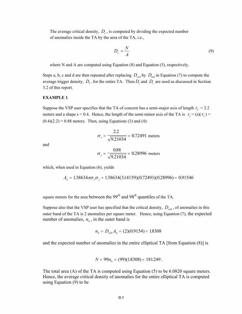
The average critical density, , is computed by dividing the expected number of anomalies inside the TA by the area of the TA, i.e.,
Dc
ANDc = (9)
where N and A are computed using Equation (8) and Equation (5), respectively.
Steps a, b, c and d are then repeated after replacing by in Equation (7) to compute the average trigger density, , for the entire TA. Then and are used as discussed in Section 3.2 of this report.
Dcob
Dc
Dtob
DtDt
EXAMPLE 1
Suppose the VSP user specifies that the TA of concern has a semi-major axis of length r = 2.2 meters and a shape s = 0.4. Hence, the length of the semi-minor axis of the TA is = (s)( ) = (0.4)(2.2) = 0.88 meters. Then, using Equations (3) and (4):
x
ry rx
σ x = =2 2
9 210340 72491
..
. meters
and
σ y = =088
9 210340 28996
..
. meters
which, when used in Equation (6), yields
A x y∆ = = =138634 138634 314159 0 72491 0 28996 0 91546. . ( . )( . )( . ) .πσ σ
square meters for the area between the 99th and 98th quantiles of the TA. Suppose also that the VSP user has specified that the critical density, , of anomalies in this outer band of the TA is 2 anomalies per square meter. Hence, using Equation (7), the expected number of anomalies, n , in the outer band is
Dcob
∆
n D Acob∆ ∆= = =( )( . ) .2 0 9154 18308
and the expected number of anomalies in the entire elliptical TA [from Equation (8)] is
N n= = =99 99 18308 181249∆ ( )( . ) . . The total area (A) of the TA is computed using Equation (5) to be 6.0820 square meters. Hence, the average critical density of anomalies for the entire elliptical TA is computed using Equation (9) to be
B.5
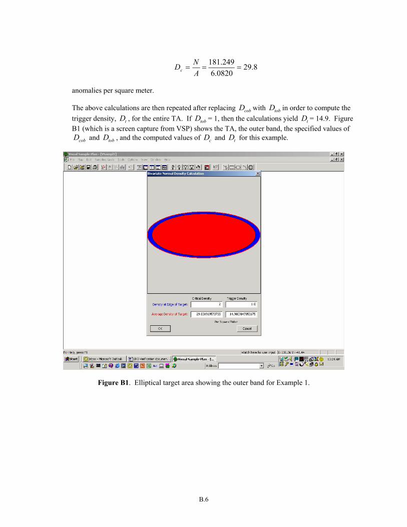
8.290820.6
249.181===
ANDc
anomalies per square meter. The above calculations are then repeated after replacing with in order to compute the trigger density, , for the entire TA. If = 1, then the calculations yield = 14.9. Figure B1 (which is a screen capture from VSP) shows the TA, the outer band, the specified values of
and , and the computed values of and for this example.
Dcob Dtob
Dt Dtob
D
Dt
Dcob Dtob c Dt
Figure B1. Elliptical target area showing the outer band for Example 1.
B.6

3. Lay down parallel transects over the study area at a random angle, θ, to the x-axis
Pick a random angle
∈
20 πθ , relative to the x-axis. The width of the swaths is w, which is selected by
the VSP user. The distance between swaths is a, which is determined by VSP. The projections of swath width and distance between swaths on the x-axis are denoted a′ and w′ , where
( )
( ) .sin
ww
sinaa
θ
θ
=′
=′
Figure B2 illustrates the swaths and the projections of their width and distance between swaths.
Figure B2. Swath edges rotated by angle θ and center of ellipse at (c, 0).
B.7
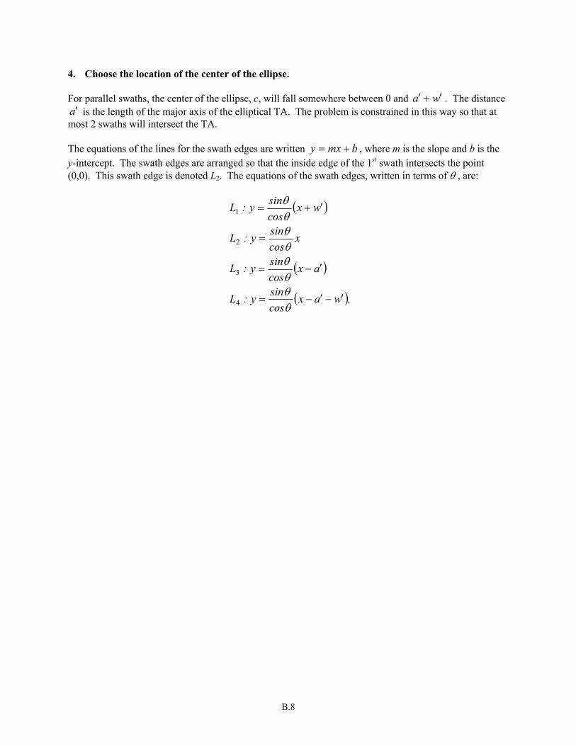
4. Choose the location of the center of the ellipse. For parallel swaths, the center of the ellipse, c, will fall somewhere between 0 and a . The distance
is the length of the major axis of the elliptical TA. The problem is constrained in this way so that at most 2 swaths will intersect the TA.
w′+′a′
The equations of the lines for the swath edges are written bmxy += , where m is the slope and b is the y-intercept. The swath edges are arranged so that the inside edge of the 1st swath intersects the point (0,0). This swath edge is denoted L2. The equations of the swath edges, written in terms of θ , are:
( )
( )
( ).waxcossiny:L
axcossiny:L
xcossiny:L
wxcossiny:L
′−′−=
′−=
=
′+=
θθθθθθθθ
4
3
2
1
B.8

5. Center the ellipse at the origin, (0,0)
This is done to simplify the limits of integration. The equations of the swath edges are now written
( )
( )
( )
( ).cwaxcossiny:L
caxcossiny:L
cxcossiny:L
cwxcossiny:L
+′−′−=
+′−=
+=
+′+=
θθθθθθθθ
4
3
2
1
Figure B3. Elliptical target area and swaths are centered about (0,0). Note that zero, one, or two swaths may intersect the ellipse (see Figure B3). In order to get the limits of integration, the equations of these lines are rewritten in terms of x:
( )
( )
( )
( ).cwaysincosx:L
caysincosx:L
cysincosx:L
wcysincosx:L
*
*
*
*
−′+′+=
−′+=
−=
′+−=
θθθθθθθθ
4
3
2
1
B.9
6. Integrate the Bivariate Normal distribution to obtain the volume, V, under the distribution curve that overlays the swaths that intersect the TA
If there are no transects intersecting the elliptical TA, this volume should be equal to zero. The actual volume represented by the intersection of the sw ths and the ellipse is approximated by integrating the BN distribution in the y-direction from
a( )yy , σσ 33− instead of setting the limits
of integration to the equation of the ellipse. This approximation overestimates the volume the farther away from the center of the ellipse the swaths intersect it. But, by doing this, we avoid having to partition the integral.
The integral to solve depends on the angle θ. If ,4
0 πθ << then solve
. ( ) ( )∫ ∫∫ ∫ −−+= x
x
x
x
L
L
L
Ldydxy,xdydxy,xV
σ
σ
σ
σφφ
3
3
3
3
3
4
1
2
If 24πθπ
<≤ ,
( ) ( ) .dxdyy,xdxdyy,xV y
y
*
*
y
y
*
*
L
L
L
L ∫ ∫∫ ∫ −−+=
σ
σ
σ
σφφ
3
3
3
3
4
3
2
1
Because we are integrating from ( )σσ 33 ,− , if the swaths do not intersect the elliptical TA, we'll still get a non-zero volume from the integral. Because the ellipse represents the 99th concentration contour of the BN distribution, there is very little volume outside its boundaries, and the over-estimation is small. An alternative approach is to manually set the volume, V, equal to zero if no transects intersect the ellipse. However, if the density of anomalies follows a BN distribution, there will be some positive number of anomalies outside the ellipse boundary.
7. Calculate the expected number of anomalies that lie within the path of the swaths within the
TA The expected number of anomalies within the swaths that cross the TA, n, is the total number of anomalies in the TA, N, multiplied by the volume of the density specified by the transects, V. The equation is
NVn = .
8. Repeat Steps 4-8 10,000 times to get a distribution for n
B.10
2.2 Case of Parallel Swaths when 2πθ =
The process described in Section 2.1 is appropriate when θ is between 0 and 2π
. When 2πθ = , then
( ) 1=θsin , so a and ′ w′ simplify to a and w, respectively. In Step 4 of Section 2.1, the swath edges are now perpendicular to the major axis of the ellipse, and so their equations become
.wax:Lax:L
x:Lwx:L
+===
−=
4
3
2
1
0
In Step 5, choose the center of the ellipse, c, between a and a + w. The center of this region is constrained so that at most two swaths intersect the ellipse. See Figure B4 for an illustration of the swath edges and the center of the ellipse. In Step 6, the equations of the swath edges become
.cwax:Lcax:L
cx:Lwcx:L
−+=−=
−=−−=
4
3
2
1
See Figure B5 for an illustration of the swath edges and the center of the ellipse when the axes have been transformed so that the center of the ellipse is located at (0,0). The equation used in Step 7 to solve for the volume of the density intersected by the swaths is
( ) ( ) .dxdyy,xdxdyy,xV x
x
y
y
L
L
L
L ∫ ∫∫ ∫ −−+=
σ
σ
σ
σφφ
3
3
3
3
4
3
2
1
B.11

Figure B4. Swath edges rotated by 2πθ = and center of ellipse ( )wa,c +∈ 0
Figure B5. Swaths translated so that center of ellipse is at (0,0).
B.12

2.3 Case of Parallel Swaths when θ = 0 When θ = 0, the swaths run parallel to the x-axis and the major axis of the ellipse. Up to this point, the swath edges have been denoted by L1, L2, L3, and L4, the distance between swaths by a or , and the width of the swaths by w or . Because of the notation used in Section 3, which considers swaths laid out in a lattice (grid) pattern, slightly different notation will be used here for the case of parallel swaths when θ = 0.
a′w′
For the case of parallel swaths and θ = 0, the swath edges will be denoted L5 through L8; the distance between swaths will be denoted b or , and the width of these swaths will be denoted v or . The distance between swaths falls in the y-axis direction, which is the direction of minor axis of the ellipse.
b′ v′
As with the special case of 2πθ = , the differences in the algorithm start in Step 4.
4. Lay down parallel swaths in an orientation perpendicular to the y-axis The width of the swaths is w. The distance between swaths is b. Because these swaths are parallel to the x-axis, there is no need to calculate projections.
5. Choose a location for the center of the ellipse
The equations of the lines for the swath edges are written so that the inside edge of the bottom swath intersects the point (0,0). For parallel swaths rotated 0 radians, the center of the ellipse will be somewhere between 0 and b + v. As before, this is done so that at most 2 swaths will intersect the elliptical TA. Figure B6 illustrates the swath edges and the center of the ellipse. The equations of the swath edges under this scenario are written
.vby:Lby:L
y:Lvy:L
+===
−=
8
7
6
5
0
6. Transform the space so that the ellipse is centered at (0,0)
As before, the coordinates are translated so the TA is centered at (0,0) for simplicity in writing the limits of integration. The results of the translation are shown in Figure B7; the equations of the swath edges are now written
.cvby:Lcby:L
cy:Lcvy:L
−+=−=
−=−−=
8
7
6
5
B.13

Figure B6. Swath edges rotated by θ = 0 and center of ellipse ( )vbcy +∈ ,0 .
Figure B7. Space translated so that center of ellipse is at (0,0).
7. Integrate out the BN distribution specified by the swaths intersecting the ellipse
The result is the volume, V, under the BN distribution defined by the intersection of the swaths and the ellipse. The equation for V is
( ) ( ) .dxdyy,xdxdyy,xV x
x
x
x
L
L
L
L ∫ ∫∫ ∫ −−+=
σ
σ
σ
σφφ
3
3
3
3
6
5
8
7
B.14
3.0 Simulation Process for Lattice (Grid) Swaths 3.1 Case of 0<θ <π / 2 for Lattice Swaths The process for lattice (perpendicular) swaths is somewhat more complicated than for parallel swaths. Steps 1- 3 are the same as for parallel swaths. The differences start in Step 4. Once an angle θ is selected
for a set of swaths, the perpendicular swaths are added at an angle of
+
2πθ
.
4. Lay down swaths at a random angle to the x-axis
The random angle the swaths are laid out relative to the x-axis is θ, where
∈
20 πθ , . As
before, the width of these swaths is specified by the VSP user to be w and the distance between the swaths is computed by VSP to be a. The projection of the swath width and distance between swaths along the x-axis are denoted w′ and a′ , where
.
sinaa
sinww
θ
θ
=′
=′
Lay down perpendicular swaths that are rotated from the x-axis by an angle of
+
2πθ
. The
swath width of these swaths is denoted v and the distance between these swaths is b. As above, the projections of the swath width and distance between swaths along the x-axis are denoted v′ and , where b′
.
sinbb
sinvv
θ
θ
=′
=′
See Figure B8 for an illustration of the swaths.
5. Choose a random center of the elliptical region
Choose the center of the ellipse (cx , cy) so that ( )wa,cx ′+′∈ 0 and c ( vb,y ′+′ )∈ 0 . As above, the assumption is that at most two swaths in either direction intersect the ellipse.
6. Transform the space so that the ellipse is centered at (0,0)
Now the equations of the swath edge lines are:
B.15
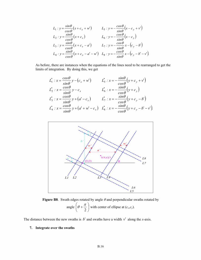
( ) ( )( ) ( )( ) ( )( ) ( ).vbcx
sincosy:Lwacx
cossiny:L
bcxsincosy:Lacx
cossiny:L
cxsincosy:Lcx
cossiny:L
vcxsincosy:Lwcx
cossiny:L
yx
yx
yx
yx
′−′−−−=′−′−+=
′−−−=′−+=
−−=+=
′+−−=′++=
θθ
θθ
θθ
θθ
θθ
θθ
θθ
θθ
84
73
62
51
As before, there are instances when the equations of the lines need to be rearranged to get the limits of integration. By doing this, we get
( ) ( )( )
( ) ( )( ) ( ).vbcy
cossinx:Lcway
sincosx:L
bcycossinx:Lcay
sincosx:L
cycossinx:Lcy
sincosx:L
vcycossinx:Lwcy
sincosx:L
y*
x*
y*
x*
y*
x*
y*
x*
′−′−+−=−′+′+=
′−+−=−′+=
+−=−=
′++−=′+−=
θθ
θθ
θθ
θθ
θθ
θθ
θθ
θθ
84
73
62
51
Figure B8. Swath edges rotated by angle θ and perpendicular swaths rotated by
angle
+
2πθ with center of ellipse at (cx,cy).
The distance between the new swaths is b′ and swaths have a width v′ along the x-axis.
7. Integrate over the swaths
B.16

This calculation is performed in a series of steps:
a. Determine the x-coordinates of the points of intersection for each of the parallel and perpendicular swaths.
b. Integrate over the swath regions. c. Integrate the corner regions. d. Calculate the total volume under the bivariate normal specified by the swaths.
Each of these steps is explained in more detail below.
a. Determine the x-coordinates of the intersection points of the swaths.
This information is needed to get the limits of integration. Begin by setting L1 = L5 to get the point x15 (see Figure B9). This gives
( ) ( )
( )
( ).sinwcosvsinccoscsinx
vcwccossinx
sincos
vcxsincoswcx
cossin
xy
yx
yx
θθθθθθθ
θθ
θθ
θθ
′+′++−=⇒
′+−′+−=⇒
′−−−=′++
15
15
1515
1
Similarly,
( )( )
( )( )( )( )
( )( )( )
( )( )
( )( )
( )( ).tanwvbtanatanccsincosx
tanwbtanatanccsincosx
sinwsinasinccoscsinx
sinwcosvsinasinccoscsinx
vbtanatanccsincosx
btanatanccsincosx
sinasinccoscsinx
cosvsinasinccoscsinx
vbtanccsincosx
cosbsinccoscsinx
sinccoscsinx
cosvsinccoscsinx
tanwvbtanccsincosx
sinwcosbsinccoscsinx
sinwsinccoscsinx
xy
xy
xy
xy
xy
xy
xy
xy
xy
xy
xy
xy
xy
xy
xy
θθθθθ
θθθθθ
θθθθθ
θθθθθθ
θθθθ
θθθθ
θθθθ
θθθθθ
θθθ
θθθθ
θθθ
θθθθ
θθθθ
θθθθθ
θθθθ
′+′+′+′+−−=
′+′+′+−−=
′−′−+−=
′−′+′−+−=
′+′+′+−−=
′+′+−−=
′−+−=
′+′−+−=
′+′+−−=
′−+−=
+−=
′++−=
′−′+′+−−=
′+′−+−=
′++−=
48
47
46
45
38
37
36
35
28
27
26
25
18
17
16
b. Integrate over the swaths.
B.17
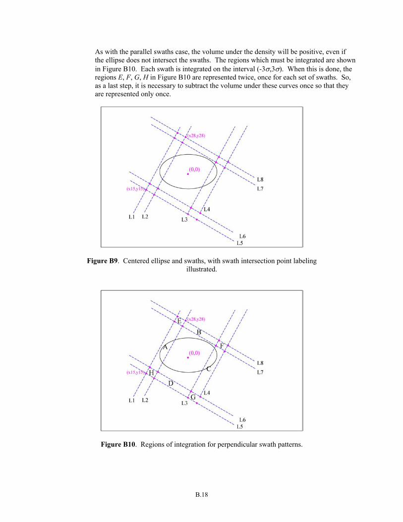
As with the parallel swaths case, the volume under the density will be positive, even if the ellipse does not intersect the swaths. The regions which must be integrated are shown in Figure B10. Each swath is integrated on the interval (-3σ,3σ). When this is done, the regions E, F, G, H in Figure B10 are represented twice, once for each set of swaths. So, as a last step, it is necessary to subtract the volume under these curves once so that they are represented only once.
Figure B9. Centered ellipse and swaths, with swath intersection point labeling illustrated.
Figure B10. Regions of integration for perpendicular swath patterns.
B.18

The order of integration and the limits of integration depend upon the angle θ. If
40 πθ << , the volumes under the BN distribution between lines (L1 and L2) and
between lines (L3 and L4) in Figure B10 are
(10) ( )∫ ∫−Φ= x
x
L
Ldydxy,xV
σ
σ
3
3121
2
(11) ( )∫ ∫−Φ= x
x
L
Ldydxy,xV
σ
σ
3
3343
4
and between lines (L5 and L6) and (L7 and L8) are
(12) ( )∫ ∫−Φ= y
y
*
*
L
Ldxdyy,xV
σ
σ
3
3566
5
(13) ( ) .dxdyy,xV y
y
*
*
L
L∫ ∫−Φ=
σ
σ
3
3788
7
If 24πθπ
<< , Equations 7 through 10 become
(14) ( )∫ ∫−Φ= y
y
*
*
L
Ldxdyy,xV
σ
σ
3
3122
1
(15) ( )∫ ∫−Φ= y
y
*
*
L
Ldxdyy,xV
σ
σ
3
3344
3
(16) ( )∫ ∫−Φ= x
x
*
*
L
Ldydxy,xV
σ
σ
3
3566
5
(17) ( ) .dydxy,xV x
x
*
*
L
L∫ ∫−Φ=
σ
σ
3
3788
7
c. Integrate over the corner regions in Figure B10.
The volumes under the corner segments must now be calculated individually so that they can be subtracted from the total volume. The order of integration for these corners depends on θ. If wvtan ′′>θ we do the integral one way; otherwise, the limits of integration change.
If wv ′′≤tanθ , then
(18) ( ) ( ) ( )∫ ∫ ∫ ∫∫ ∫ Φ+Φ+Φ= 18
27
1
2
28
18
8
2
27
17
1
7
x
x
L
L
x
x
L
L
x
x
L
LE dydxy,xdydxy,xdydxy,xV
(19) ( ) ( ) ( )∫ ∫ ∫ ∫∫ ∫ Φ+Φ+Φ= 38
47
3
4
48
38
8
4
47
37
3
7
x
x
L
L
x
x
L
L
x
x
L
LF dydxy,xdydxy,xdydxy,xV
(20) ( ) ( ) ( )∫ ∫ ∫ ∫∫ ∫ Φ+Φ+Φ= 36
45
3
4
46
36
6
4
45
35
3
5
x
x
L
L
x
x
L
L
x
x
L
LG dydxy,xdydxy,xdydxy,xV
B.19

(21) ( ) ( ) ( )∫ ∫ ∫ ∫∫ ∫ Φ+Φ+Φ= 16
25
1
2
26
16
6
2
25
15
1
5
x
x
L
L
x
x
L
L
x
x
L
LH .dydxy,xdydxy,xdydxy,xV
If wv ′′>tanθ , the corner volumes are calculated as follows:
(22) ( ) ( ) ( )∫ ∫ ∫ ∫∫ ∫ Φ+Φ+Φ= 27
18
8
7
28
27
8
2
18
17
1
7
x
x
L
L
x
x
L
L
x
x
L
LE dydxy,xdydxy,xdydxy,xV
(23) ( ) ( ) ( )∫ ∫ ∫ ∫∫ ∫ Φ+Φ+Φ= 47
38
8
7
48
47
8
4
38
37
3
7
x
x
L
L
x
x
L
L
x
x
L
LF dydxy,xdydxy,xdydxy,xV
(24) ( ) ( ) ( )∫ ∫ ∫ ∫∫ ∫ Φ+Φ+Φ= 45
36
6
5
46
45
6
4
36
35
3
5
x
x
L
L
x
x
L
L
x
x
L
LG dydxy,xdydxy,xdydxy,xV
(25) ( ) ( ) ( )∫ ∫ ∫ ∫∫ ∫ Φ+Φ+Φ= 25
16
6
5
26
25
6
2
16
15
1
5
x
x
L
L
x
x
L
L
x
x
L
LH .dydxy,xdydxy,xdydxy,xV
d. Calculate the total volume.
The total volume is then V = V12 + V34 + V56 + V78 – VE – VF – VG - VH. As in the case of only parallel swaths, because we are integrating over the y region from (-3σy,3σy), we slightly overestimate the volume under the density.
8. Calculate the number of objects inside the swaths
The expected number of anomalies inside the area covered by regions A through G is the total number of items, N, multiplied by the volume of the density represented by those regions, V. The equation for the expected number of anomalies is
NVn = .
Repeat Steps 4 through 8 10,000 times to get a distribution for n.
3.2 Case of θ = 0 for Lattice Swaths In VSP, the major axis (denoted a) is always oriented along the x-axis; the minor axis (denoted b) is always oriented along the y-axis. Therefore, when considering special cases of lattice swaths, we only need consider the rotation of θ = 0. As expected, this case is a combination of the special cases for parallel swaths. As with the special cases of parallel swaths, the differences in the algorithm start in Step 4.
4. Lay down swaths parallel to the x- and y-axes The set of swaths which run parallel to the x-axis have swath edges denotes L1 through L4; the width of these swaths is denoted w. These swaths are distance a apart. The swath edges of the intersecting perpendicular swaths have edges denoted L5 through L8; the swaths have width v and distance between swaths b. As before, the line representing the right edge of the leftmost swath, L2, intersects (0,0); see Figure B10. The equations of the lines representing the swath edges are:
B.20

.vby:Lwax:Lby:Lax:L
y:Lx:Lvy:Lwx:L
+=+=====
−=−=
84
73
62
51
00
5. Choose a random center of the elliptical region
Choose the center of the ellipse (cx,cy) so that ( )wa,cx +∈ 0 and ( )vb,cy +∈ 0 . As before, we do this so that at most two swaths intersect the ellipse. See Figure B12.
6. Transform the space so that the ellipse is centered at (0,0)
The ellipse is centered at (0,0) by subtracting cx from lines L1 through L4 and subtracting cy from lines L5 through L8. The equations of these lines now become
.cvby:Lcwax:Lcby:Lcax:L
cy:Lcx:Lcvy:Lcwx:L
yx
yx
yx
yx
−+=−+=−=−=
−=−=−−=−−=
84
73
62
51
The results of the translation are shown in Figure B13.
Figure B11. Perpendicular swaths rotated by angle θ = 0.
B.21
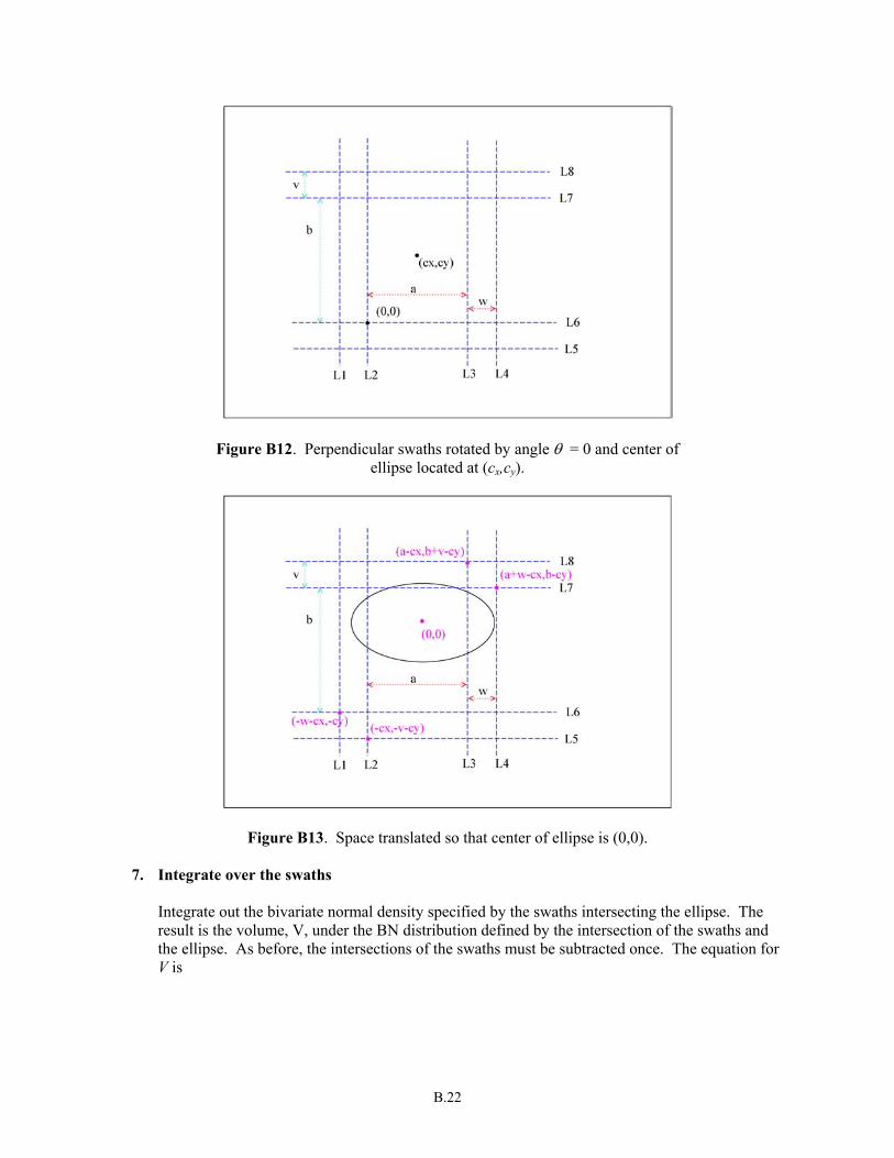
Figure B12. Perpendicular swaths rotated by angle θ = 0 and center of ellipse located at (cx,cy).
Figure B13. Space translated so that center of ellipse is (0,0).
7. Integrate over the swaths Integrate out the bivariate normal density specified by the swaths intersecting the ellipse. The result is the volume, V, under the BN distribution defined by the intersection of the swaths and the ellipse. As before, the intersections of the swaths must be subtracted once. The equation for V is
B.22

V =
(26)
( ) ( )
( ) ( )
( ) ( )
( ) ( )∫ ∫∫ ∫
∫ ∫∫ ∫
∫ ∫∫ ∫
∫ ∫∫ ∫
Φ−Φ
−Φ−Φ
−Φ+Φ
+Φ+Φ
−−
−−
4
3
8
7
2
1
8
7
4
3
6
5
2
1
6
5
8
7
6
5
4
3
2
1
3
3
3
3
3
3
3
3
L
L
L
L
L
L
L
L
L
L
L
L
L
L
L
L
L
L
L
L
L
L
L
L
.dydxy,xdydxy,x
dydxy,xdydxy,x
dydxy,xdydxy,x
dxdyy,xdxdyy,x
x
x
x
x
y
y
y
y
σ
σ
σ
σ
σ
σ
σ
σ
B.23
APPENDIX C
Algorithms Used in VSP to Compute the Probability that Meandering Transects Traverse and Detect a Target Area

APPENDIX C
Algorithms Used in VSP to Compute the Probability that Meandering Transects Traverse and Detect a Target Area
John E. Wilson
Statistical and Quantitative Sciences Pacific Northwest National Laboratory
Richland, WA
1.0 Area of Polygon Intersecting Circle Algorithm Finding the area of intersection between a circle and a polygon (see the red area in Figure C1) is a complicated problem. To make the problem manageable, VSP breaks the problem into two steps.
Figure C1. Area of intersection between a circle and a polygon. Step one is to break the polygon into non-overlapping triangles (see Figure C2). Any polygon that doesn’t intersect itself can be decomposed into a set of non-overlapping triangles. See documentation of Triangulate algorithm in Section C5 for details.
Figure C2. Breaking the polygon into non-overlapping triangles.
C.1

Step two is to find the area of intersection between each individual triangle and the circle. The area of intersection between the circle and the polygon is the sum of the intersections with the individual triangles. See documentation of the Triangle Circle Area algorithm in Section C6 for details.
C.2

2.0 Polygon Intersecting Polygon Algorithm The purpose of this algorithm is to find the intersection between two polygons (A and B). The intersection (if it exists) will be a new polygon (C in Figure C3). This algorithm assumes that the two polygons have no interior holes and that they do not intersect themselves (one segment of a polygon does not intersect another segment of the same polygon).
Figure C3. The intersection, C, between Polygons A and B.
First a quick check is made on the extents of the two polygons. For instance, if the maximum Y coordinate of A is less than the minimum Y coordinate of B, then the algorithm returns a value of false (no intersection).
Figure C4. The intersection, C, between Polygons A and B. The next step is to intersect Polygon A with Polygon B. Each segment of A is checked for intersections with B to find intersection points (see Figure C4). Every original point (P1, P2, P3, P4) and intersection point (P5, P6, P7, P8, P9, P10) is put into List A in correct order. The process is as follows:
1. P1 is added to List A 2. Each segment of A (P1-P2, etc.) is checked 3. Each segment of B is checked for intersections with the segment of A
C.3
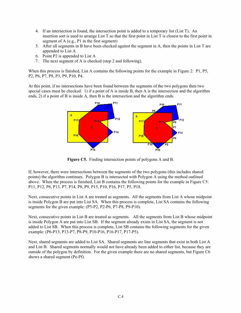
4. If an intersection is found, the intersection point is added to a temporary list (List T). An insertion sort is used to arrange List T so that the first point in List T is closest to the first point in segment of A (e.g., P1 in the first segment)
5. After all segments in B have been checked against the segment in A, then the points in List T are appended to List A
6. Point P2 is appended to List A 7. The next segment of A is checked (step 2 and following).
When this process is finished, List A contains the following points for the example in Figure 2: P1, P5, P2, P6, P7, P8, P3, P9, P10, P4.
At this point, if no intersections have been found between the segments of the two polygons then two special cases must be checked: 1) if a point of A is inside B, then A is the intersection and the algorithm ends, 2) if a point of B is inside A, then B is the intersection and the algorithm ends.
Figure C5. Finding intersection points of polygons A and B.
If, however, there were intersections between the segments of the two polygons (this includes shared points) the algorithm continues. Polygon B is intersected with Polygon A using the method outlined above. When the process is finished, List B contains the following points for the example in Figure C5: P11, P12, P6, P13, P7, P14, P8, P9, P15, P10, P16, P17, P5, P18.
Next, consecutive points in List A are treated as segments. All the segments from List A whose midpoint is inside Polygon B are put into List SA. When this process is complete, List SA contains the following segments for the given example: (P5-P2, P2-P6, P7-P8, P9-P10).
Next, consecutive points in List B are treated as segments. All the segments from List B whose midpoint is inside Polygon A are put into List SB. If the segment already exists in List SA, the segment is not added to List SB. When this process is complete, List SB contains the following segments for the given example: (P6-P13, P13-P7, P8-P9, P10-P16, P16-P17, P17-P5).
Next, shared segments are added to List SA. Shared segments are line segments that exist in both List A and List B. Shared segments normally would not have already been added to either list, because they are outside of the polygon by definition. For the given example there are no shared segments, but Figure C6 shows a shared segment (Pe-Pf).
C.4

Figure C6. Example of a shared segment (Pe-Pf).
Next, orphan segments must be removed from List SA and List SB. Orphan segments are those that have at least one point that is not used by another segment. The process is as follows:
1. Each segment in List SA is checked 2. The endpoints of the segment to be checked are Px and Py. Found1 and Found2 are set to false 3. If Px is used by another segment in List SA or List SB, then Found1 is set to true 4. If Py is used by another segment in List SA or List SB, then Found2 is set to true 5. If Found1 or Found2 is false, then the segment Px-Py is an orphan and is removed from List SA
and the entire process is performed again (Step 1 and following). Otherwise, the process continues with step 6
6. Each segment in List SB is checked 7. The endpoints of the segment to be checked are Px and Py. Found1 and Found2 are set to false 8. If Px is used by another segment in List SA or List SB then Found1 is set to true 9. If Py is used by another segment in List SA or List SB then Found2 is set to true 10. If Found1 or Found2 is false, then the segment Px-Py is an orphan and is removed from List SB
and entire process is performed again (step 1 and following) 11. If Found1 and Found2 are true, then there are no more orphans and the process is complete.
Finally, the segments in List SA and List SB must be combined into a new polygon. This process is as follows:
1. The new polygon, C, contains no points to begin with 2. If List SA has any segments in it, the first segment (Px-Py) is removed from it. If List SA does
not have any segments, then the first segment (Px-Py) is removed from List SB. Point Px is added to C. Nextpnt is set to Py
3. Each segment (Px-Py) in List SA is checked for a point matching Nextpnt 4. If Px matches Nextpnt, then Nextpnt is added to C, Nextpnt is set to Py, and processing continues
with Step 3 5. If Py matches Nextpnt, then Nextpnt is added to C, Nextpnt is set to Px, and processing continues
with Step 3 6. If neither Px nor Py matches Nextpnt, then the next segment in List SA is checked (Step 3 and
following) 7. After all segments in List SA have been checked and a matching point has still not been found,
the process is repeated with List SB (Step 8 and following) 8. Each segment (Px-Py) in List SB is checked for a point matching Nextpnt
C.5
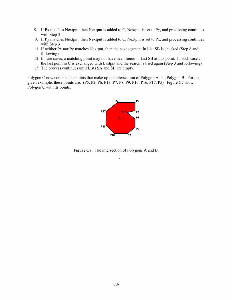
9. If Px matches Nextpnt, then Nextpnt is added to C, Nextpnt is set to Py, and processing continues with Step 3
10. If Py matches Nextpnt, then Nextpnt is added to C, Nextpnt is set to Px, and processing continues with Step 3
11. If neither Px nor Py matches Nextpnt, then the next segment in List SB is checked (Step 8 and following)
12. In rare cases, a matching point may not have been found in List SB at this point. In such cases, the last point in C is exchanged with Lastpnt and the search is tried again (Step 3 and following)
13. The process continues until Lists SA and SB are empty.
Polygon C now contains the points that make up the intersection of Polygon A and Polygon B. For the given example, these points are: (P5, P2, P6, P13, P7, P8, P9, P10, P16, P17, P5). Figure C7 show Polygon C with its points.
Figure C7. The intersection of Polygons A and B.
.
C.6
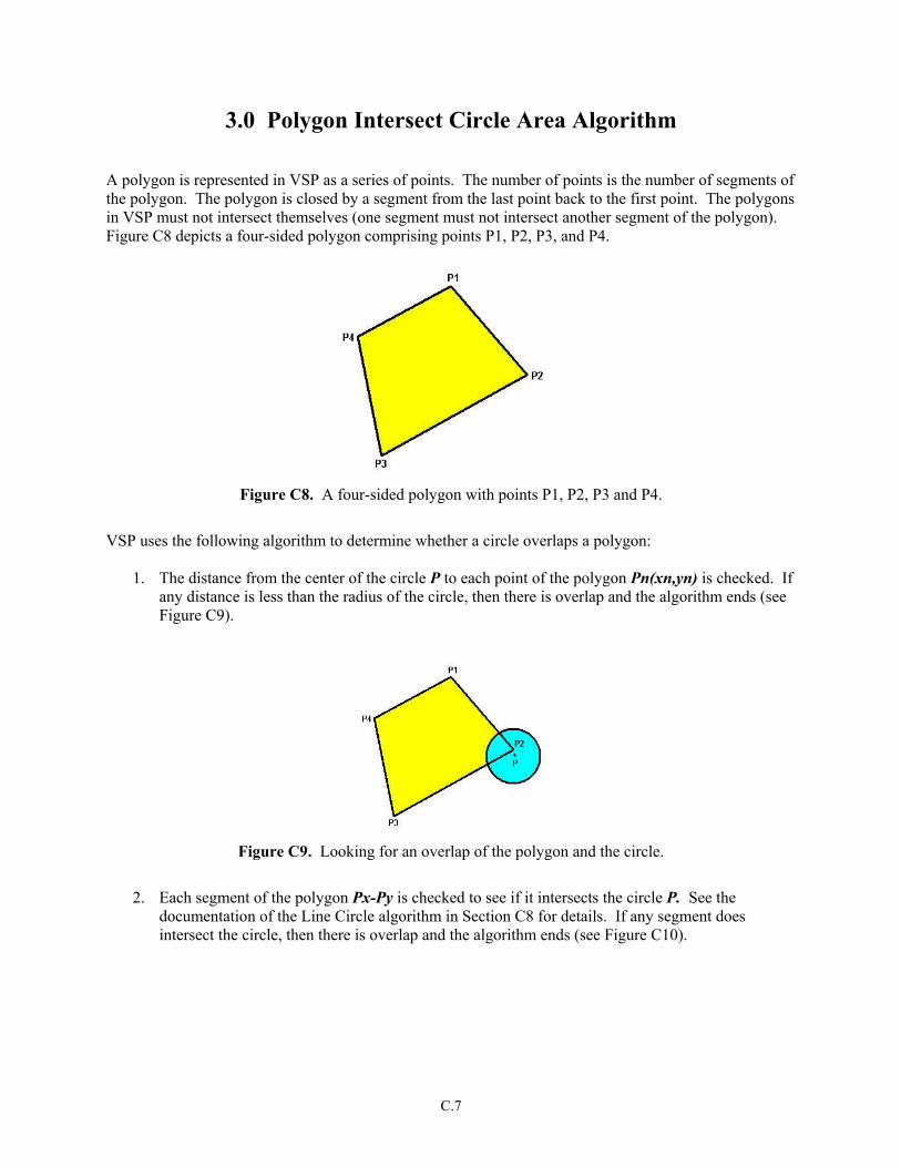
3.0 Polygon Intersect Circle Area Algorithm A polygon is represented in VSP as a series of points. The number of points is the number of segments of the polygon. The polygon is closed by a segment from the last point back to the first point. The polygons in VSP must not intersect themselves (one segment must not intersect another segment of the polygon). Figure C8 depicts a four-sided polygon comprising points P1, P2, P3, and P4.
Figure C8. A four-sided polygon with points P1, P2, P3 and P4.
VSP uses the following algorithm to determine whether a circle overlaps a polygon:
1. The distance from the center of the circle P to each point of the polygon Pn(xn,yn) is checked. If
any distance is less than the radius of the circle, then there is overlap and the algorithm ends (see Figure C9).
Figure C9. Looking for an overlap of the polygon and the circle.
2. Each segment of the polygon Px-Py is checked to see if it intersects the circle P. See the
documentation of the Line Circle algorithm in Section C8 for details. If any segment does intersect the circle, then there is overlap and the algorithm ends (see Figure C10).
C.7

Figure C10. Looking for an intersection between a transect segment and the circle.
3. Finally, if the center of the circle P is inside the polygon (see documentation of Inside Polygon
algorithm in Section C9 for details), then there is overlap and the algorithm ends (see Figure C11). If the center of the circle P is not inside the polygon, then there is no overlap and the algorithm ends.
Figure C11. Looking to see if the center of the circle is inside the polygon.
C.8
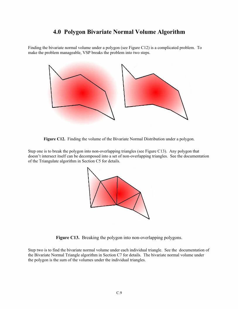
4.0 Polygon Bivariate Normal Volume Algorithm Finding the bivariate normal volume under a polygon (see Figure C12) is a complicated problem. To make the problem manageable, VSP breaks the problem into two steps.
Figure C12. Finding the volume of the Bivariate Normal Distribution under a polygon.
Step one is to break the polygon into non-overlapping triangles (see Figure C13). Any polygon that doesn’t intersect itself can be decomposed into a set of non-overlapping triangles. See the documentation of the Triangulate algorithm in Section C5 for details.
Figure C13. Breaking the polygon into non-overlapping polygons.
Step two is to find the bivariate normal volume under each individual triangle. See the documentation of the Bivariate Normal Triangle algorithm in Section C7 for details. The bivariate normal volume under the polygon is the sum of the volumes under the individual triangles.
C.9

5.0 Triangulate Algorithm A polygon is represented in VSP as a series of points (vertices). The number of points is the number of segments of the polygon. The polygon is closed by a segment from the last point back to the first point. VSP uses the following algorithm to convert this list of points into a set of non-overlapping triangles.
1. Determine whether the polygon has a clockwise or a counter-clockwise orientation. If A < 0, then the polygon has a clockwise orientation. If A > 0, then the polygon has a counter-clockwise orientation, where
∑=
++ −=n
iiiii xyyxA
111 )(
n = the number of points in the polygon xi = the x coordinate of the ith point yi = is the y coordinate of the ith point
2. If the polygon has more than 3 points, find and remove the best triangle from the point list using
Steps 3 through 8 below. The best triangle to remove is the smallest triangle comprising consecutive points remaining in the point list that is oriented in the same direction as the original polygon and encloses no other points in the list.
3. The best triangle (k) and best size (Sk) are reset. 4. Perform Steps 5 through 8 for each point (i) in the polygon list, setting the current triangle to
check using the (i-1), (i) and (i+1) points as the vertices of the triangle. 5. The orientation of the triangle is checked to see if it is oriented in the same direction as the
original polygon. If not, the next triangle is checked (Step 4 and following). If d < 0, then the triangle has a clockwise orientation. If d > 0, then the triangle has a counter-clockwise orientation, where:
))(())(( 111111 −+−−+− −−−−−= iiiiiiii xxyyyyxxd
6. Each point (j) in the polygon list is checked to see if it is contained inside the triangle. If the point
is contained, the next triangle is checked (Step 4 and following). This is accomplished by checking the orientation of the 3 sub-triangles: (i, i-1, j), (i-1, i+1, j), and (i+1, i, j). If each of those 3 sub-triangles is oriented in the opposite direction of the original polygon then the point is contained by the triangle.
7. The size of the current triangle (Si) is checked against the best size (Sk). If Si < Sk, then Sk is set to Si and k is set to i.
2
112
11 )()( +−+− −+−= iiiii yyxxS
8. After all triangles have been checked (Steps 4 through 7), then point k is removed from the polygon list of points, and the best triangle (k-1, k, k+1) is added to the list of triangles.
9. The next best triangle in the polygon list is found and removed (Step 2 and following). 10. When only 3 points remain in the polygon list, those points are added to the list of new triangles
and the algorithm is complete.
C.10
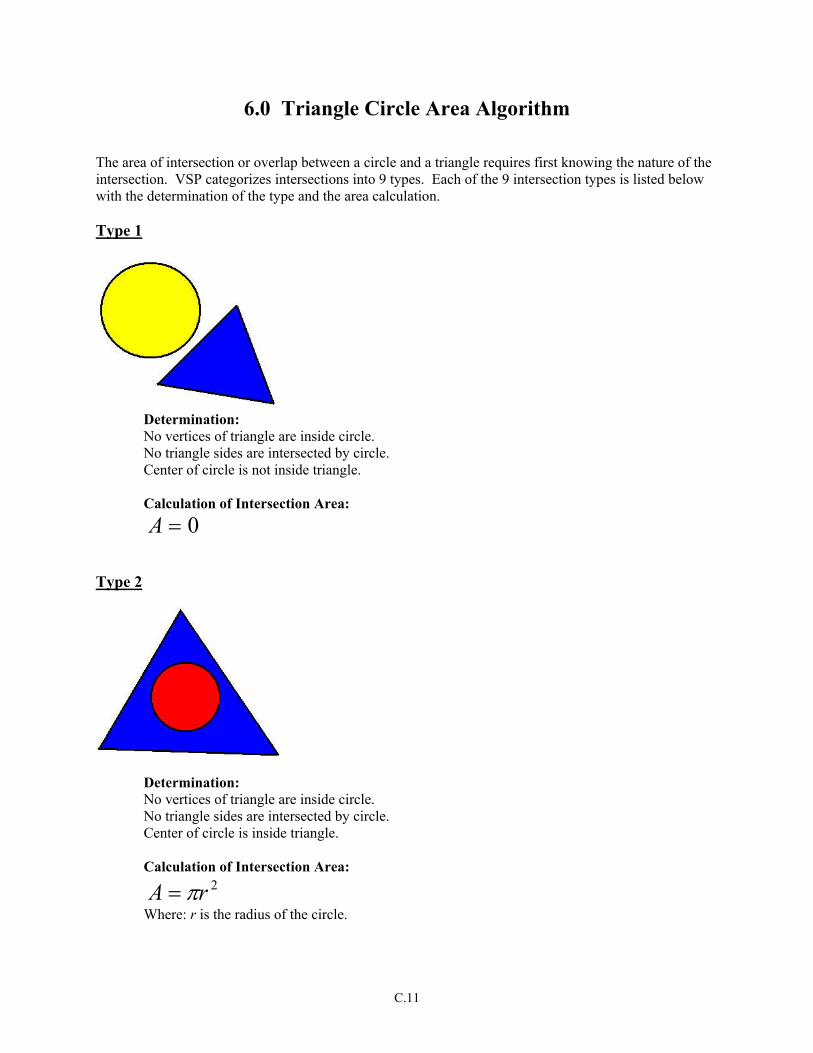
6.0 Triangle Circle Area Algorithm The area of intersection or overlap between a circle and a triangle requires first knowing the nature of the intersection. VSP categorizes intersections into 9 types. Each of the 9 intersection types is listed below with the determination of the type and the area calculation. Type 1
Determination: No vertices of triangle are inside circle. No triangle sides are intersected by circle. Center of circle is not inside triangle. Calculation of Intersection Area:
0=A Type 2
Determination: No vertices of triangle are inside circle. No triangle sides are intersected by circle. Center of circle is inside triangle. Calculation of Intersection Area:
2rA π= Where: r is the radius of the circle.
C.11

Type 3
Determination: All vertices of triangle are inside circle. Calculation of Intersection Area: The area of the triangle is calculated using the following general area equation for a polygon:
∑=
++ −=n
iiiii yxyxA
111 )( (C1)
n is the number of points in the polygon xi is the x coordinate of the ith point yi is the y coordinate of the ith point
Type 4
Determination: Two vertices of the triangle are inside the circle.
Calculation of Intersection Area: The area of intersection is the sum of the area of quadrangle BCXY and the area of the circle segment XYr. The area of the quadrangle is found using Equation C1. The intersection points X and Y are found using the Line Circle Algorithm, which is documented in Section C7. The area of the circle segment XYr is calculated as:
C.12

2212 cos drdrdrA −−
= − (C2)
where:
( )2
)()(4 222YXYX yyxxr
d−+−−−
=
xx is the x coordinate of point X yx is the y coordinate of point X xy is the x coordinate of point Y yy is the y coordinate of point Y r is the radius of the circle
Type 5
Determination: One vertex of triangle is inside circle. Two sides of triangle intersect circle. Calculation of Intersection Area: The area of intersection is the sum of the area of the triangle AXY(Equation C1) and the area of the circle segment XYr (Equation C2).
Type 6
Determination:
C.13
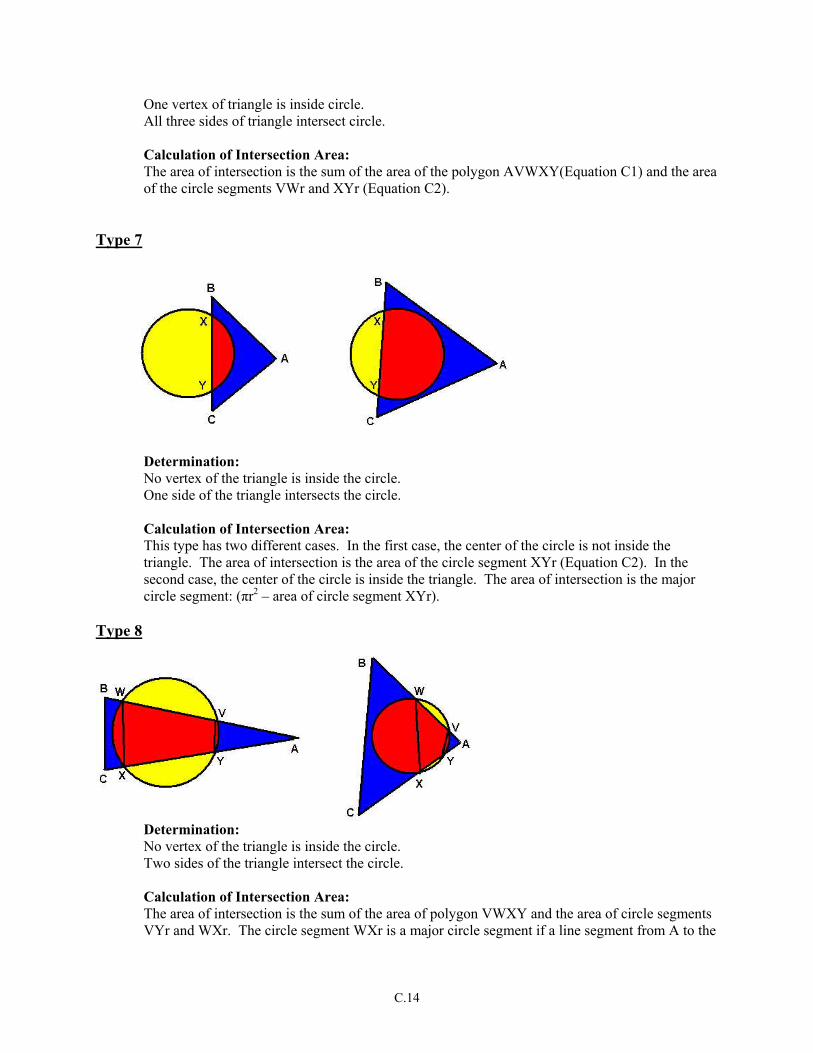
One vertex of triangle is inside circle. All three sides of triangle intersect circle. Calculation of Intersection Area: The area of intersection is the sum of the area of the polygon AVWXY(Equation C1) and the area of the circle segments VWr and XYr (Equation C2).
Type 7
Determination: No vertex of the triangle is inside the circle. One side of the triangle intersects the circle. Calculation of Intersection Area: This type has two different cases. In the first case, the center of the circle is not inside the triangle. The area of intersection is the area of the circle segment XYr (Equation C2). In the second case, the center of the circle is inside the triangle. The area of intersection is the major circle segment: (πr2 – area of circle segment XYr).
Type 8
Determination: No vertex of the triangle is inside the circle. Two sides of the triangle intersect the circle. Calculation of Intersection Area: The area of intersection is the sum of the area of polygon VWXY and the area of circle segments VYr and WXr. The circle segment WXr is a major circle segment if a line segment from A to the
C.14
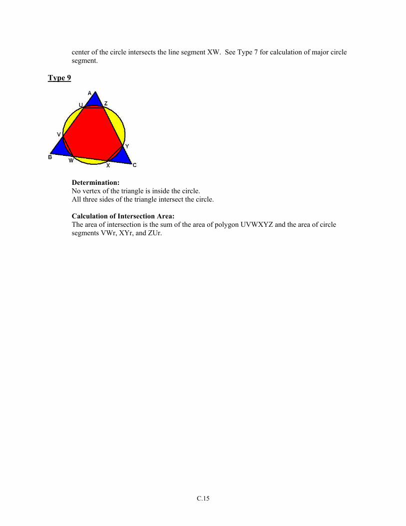
center of the circle intersects the line segment XW. See Type 7 for calculation of major circle segment.
Type 9
Determination: No vertex of the triangle is inside the circle. All three sides of the triangle intersect the circle. Calculation of Intersection Area: The area of intersection is the sum of the area of polygon UVWXYZ and the area of circle segments VWr, XYr, and ZUr.
C.15

7.0 Bivariate Normal Triangle Algorithm The bivariate normal volume under a triangle is calculated using the following method. The triangle is defined by three points and three lines. The points of the triangle are sorted by ascending x coordinate so that it is arranged similarly to the triangle in Figure C14.
Figure C14. The three points and three lines of a triangle.
The volume is calculated as follows:
∫ ∫∫ ∫ += 3
2
2
3
2
1
1
3
),(),(x
x
L
L
x
x
L
LdydxyxdydxyxV φφ
where:
333
222
111
:::
bxmyLbxmyLbxmyL
+=+=+=
12
121 xx
yym−−
=
23
232 xx
yym
−−
=
13
133 xx
yym
−−
=
1111 xmyb −=
2222 xmyb −=
C.16
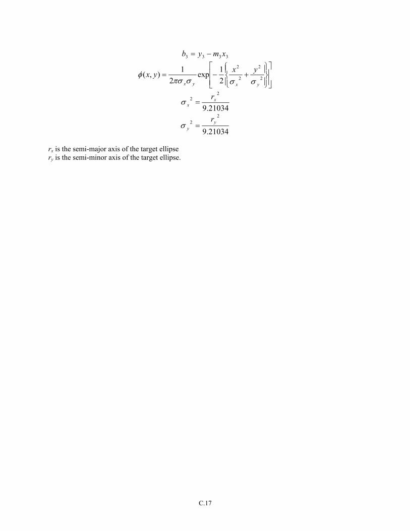
3333 xmyb −=
+−= 2
2
2
2
21exp
21),(
yxyx
yxyxσσσπσ
φ
21034.9
22 x
xr
=σ
21034.9
22 y
y
r=σ
rx is the semi-major axis of the target ellipse ry is the semi-minor axis of the target ellipse.
C.17
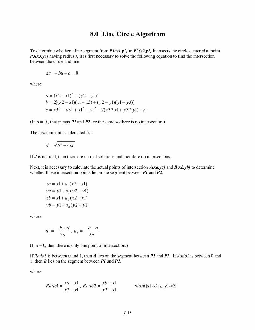
8.0 Line Circle Algorithm To determine whether a line segment from P1(x1,y1) to P2(x2,y2) intersects the circle centered at point P3(x3,y3) having radius r, it is first necessary to solve the following equation to find the intersection between the circle and line:
02 =++ cbuau where:
22 )12()12( yyxxa −+−= )]31)(12()31)(12[(2 yyyyxxxxb −−+−−=
22222 )1*31*3(21133 ryyxxyxyxc −+−+++=
(If , that means P1 and P2 are the same so there is no intersection.) 0=a The discriminant is calculated as:
acbd 42 −= If d is not real, then there are no real solutions and therefore no intersections. Next, it is necessary to calculate the actual points of intersection A(xa,ya) and B(xb,yb) to determine whether those intersection points lie on the segment between P1 and P2:
)12(1 1 xxuxxa −+= )12(1 1 yyuyya −+= )12(1 2 xxuxxb −+= )12(1 2 yyuyyb −+=
where:
adbu
21+−
= , a
db22
−−=u
(If d = 0, then there is only one point of intersection.) If Ratio1 is between 0 and 1, then A lies on the segment between P1 and P2. If Ratio2 is between 0 and 1, then B lies on the segment between P1 and P2. where:
1211
xxxxaRatio
−−
= , 1212
xxxxbRatio
−−
= when |x1-x2| ≥ |y1-y2|
C.18

1211
yyyyaRatio
−−
= , 1212
yyyybRatio
−−
= when |x1-x2| < |y1-y2|.
If A or B lies on the segment between P1 and P2, then the circle intersects the line segment, otherwise the circle does not intersect the line segment.
C.19
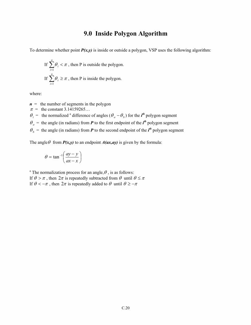
9.0 Inside Polygon Algorithm To determine whether point P(x,y) is inside or outside a polygon, VSP uses the following algorithm:
If ∑ , then P is outside the polygon. πθ <=
n
ii
1
If ∑ , then P is inside the polygon. πθ ≥=
n
ii
1
where: n = the number of segments in the polygon π = the constant 3.14159265…
iθ = the normalized a difference of angles ( ba θθ − ) for the ith polygon segment
aθ = the angle (in radians) from P to the first endpoint of the ith polygon segment
bθ = the angle (in radians) from P to the second endpoint of the ith polygon segment The angleθ from P(x,y) to an endpoint A(ax,ay) is given by the formula:
−−
= −
xaxyay1tanθ
a The normalization process for an angle,θ , is as follows: If πθ > , then π2 is repeatedly subtracted from θ until πθ ≤ If πθ −< , then π2 is repeatedly added to θ until πθ −≥
C.20
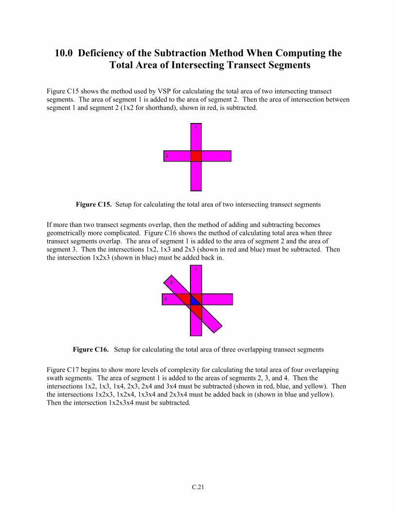
10.0 Deficiency of the Subtraction Method When Computing the Total Area of Intersecting Transect Segments
Figure C15 shows the method used by VSP for calculating the total area of two intersecting transect segments. The area of segment 1 is added to the area of segment 2. Then the area of intersection between segment 1 and segment 2 (1x2 for shorthand), shown in red, is subtracted.
Figure C15. Setup for calculating the total area of two intersecting transect segments
If more than two transect segments overlap, then the method of adding and subtracting becomes geometrically more complicated. Figure C16 shows the method of calculating total area when three transect segments overlap. The area of segment 1 is added to the area of segment 2 and the area of segment 3. Then the intersections 1x2, 1x3 and 2x3 (shown in red and blue) must be subtracted. Then the intersection 1x2x3 (shown in blue) must be added back in.
Figure C16. Setup for calculating the total area of three overlapping transect segments
Figure C17 begins to show more levels of complexity for calculating the total area of four overlapping swath segments. The area of segment 1 is added to the areas of segments 2, 3, and 4. Then the intersections 1x2, 1x3, 1x4, 2x3, 2x4 and 3x4 must be subtracted (shown in red, blue, and yellow). Then the intersections 1x2x3, 1x2x4, 1x3x4 and 2x3x4 must be added back in (shown in blue and yellow). Then the intersection 1x2x3x4 must be subtracted.
C.21

Figure C17. Setup for calculating the total area of four overlapping transect segments.
Because each added swath geometrically increases the complexity of calculating the total area, VSP ignores overlaps beyond the first overlap. This may cause the area (Att) to be smaller than it should be when multiple overlaps exist. Combining the overlapping transect segments into a single complex polygon has been considered. Because of the complexities resulting from possible interior holes (see Figure C18), this method has not been implemented yet. If the Polygon Intersection algorithm can be adapted to accommodate and produce interior holes, this method will prove most effective.
Figure C18. An interior hole of overlapping transects.
C.22
PNNL-14267
Distribution No. of No. of Copies Copies OFFSITE 4 SERDP
SERDP Program Office, Suite 303 901 N. Stuart Street Arlington, VA 22203 A. Andrews J. Fairbanks J. Marqusee B. Smith
5 EPA
Ariel Rios Building 1200 Pennsylvania Avenue, N.W. Washington, DC 20460
M. Carter, 5106G D. Crumbling, 5102G T. Jover, 5103T J. Warren, 2811R L. Zaragoza, 5202G
DOE D. Bottrell
19901 Germantown Rd. Germantown, MD 20874-1290
2 DoD J. Sample
NAVSEA 04XQ 1661 Redbank Rd Suite 104 Goose Creek, SC 29445-6511
R. Young USACE PO Box 1600 Huntsville, AL 35807-4301
2 Gannett Fleming
6242 Hidden Woods Court Apt. T-2 Springfield, VA 22152
N. Lantzer L. Wrench ONSITE DOE, RL E.M. Bowers A2-15 16 Pacific Northwest National Laboratory D.J. Bates K5-12 D.K. Carlson K5-12 R.O. Gilbert (5) K5-12 N.L. Hassig K5-12 C.A. McKinstry K5-12 R.F. O’Brien K5-12 B.A. Pulsipher (5) K5-12 J.E. Wilson K5-12
Distr.1