Versatile and scalable cosparse methods for physics … · Versatile and scalable cosparse methods...
41
HAL Id: hal-01496767 https://hal.inria.fr/hal-01496767v2 Submitted on 16 Jul 2017 HAL is a multi-disciplinary open access archive for the deposit and dissemination of sci- entific research documents, whether they are pub- lished or not. The documents may come from teaching and research institutions in France or abroad, or from public or private research centers. L’archive ouverte pluridisciplinaire HAL, est destinée au dépôt et à la diffusion de documents scientifiques de niveau recherche, publiés ou non, émanant des établissements d’enseignement et de recherche français ou étrangers, des laboratoires publics ou privés. Versatile and scalable cosparse methods for physics-driven inverse problems Srđan Kitić, Siouar Bensaid, Laurent Albera, Nancy Bertin, Rémi Gribonval To cite this version: Srđan Kitić, Siouar Bensaid, Laurent Albera, Nancy Bertin, Rémi Gribonval. Versatile and scalable cosparse methods for physics-driven inverse problems. 2017. <hal-01496767v2>
Transcript of Versatile and scalable cosparse methods for physics … · Versatile and scalable cosparse methods...

HAL Id: hal-01496767https://hal.inria.fr/hal-01496767v2
Submitted on 16 Jul 2017
HAL is a multi-disciplinary open accessarchive for the deposit and dissemination of sci-entific research documents, whether they are pub-lished or not. The documents may come fromteaching and research institutions in France orabroad, or from public or private research centers.
L’archive ouverte pluridisciplinaire HAL, estdestinée au dépôt et à la diffusion de documentsscientifiques de niveau recherche, publiés ou non,émanant des établissements d’enseignement et derecherche français ou étrangers, des laboratoirespublics ou privés.
Versatile and scalable cosparse methods forphysics-driven inverse problems
Srđan Kitić, Siouar Bensaid, Laurent Albera, Nancy Bertin, Rémi Gribonval
To cite this version:Srđan Kitić, Siouar Bensaid, Laurent Albera, Nancy Bertin, Rémi Gribonval. Versatile and scalablecosparse methods for physics-driven inverse problems. 2017. <hal-01496767v2>

Versatile and scalable cosparse methods forphysics-driven inverse problems
Srdan Kitic, Siouar Bensaid, Laurent Albera, Nancy Bertin and Remi Gribonval
Abstract Solving an underdetermined inverse problem implies the use of a regular-ization hypothesis. Among possible regularizers, the so-called sparsity hypothesis,described as a synthesis model of the signal of interest from a low number of ele-mentary signals taken in a dictionary, is now widely used. In many inverse problemsof this kind, it happens that an alternative model, the cosparsity hypothesis (statingthat the result of some linear analysis of the signal is sparse), offers advantageousproperties over the classical synthesis model. A particular advantage is its ability tointrinsically integrate physical knowledge about the observed phenomenon, whicharises naturally in the remote sensing contexts through some underlying partial dif-ferential equation. In this chapter, we illustrate on two worked examples (acous-tic source localization and brain source imaging) the power of a generic cosparseapproach to a wide range of problems governed by physical laws, how it can beadapted to each of these problems in a very versatile fashion, and how it can scaleup to large volumes of data typically arising in applications.
Srdan KiticTechnicolor, Cesson-Sevigne, e-mail: [email protected]
Siouar BensaidUniversite de Rennes 1 (LTSI), Rennes, e-mail: [email protected]
Laurent AlberaUniversite de Rennes 1 (LTSI), Rennes, e-mail: [email protected]
Nancy BertinIRISA, Rennes, e-mail: [email protected]
Remi GribonvalInria Rennes - Bretagne Atlantique, Rennes, e-mail: [email protected]
This work was supported in part by the European Research Council, PLEASE project (ERC-StG-2011-277906).
1

2 Srdan Kitic, Siouar Bensaid, Laurent Albera, Nancy Bertin and Remi Gribonval
1 Introduction
Inverse source problems consist in inferring information from an object in an indi-rect manner, through the signals it emits or scatters. This covers in particular remotesensing, a term coined in Earth sciences [12], to indicate acquisition of shape orstructure data of the Earth’s crust, using signal processing techniques. More gen-erally, remote sensing considers any method that collects distant observations froman object, with a variety of possible signal modalities and imaging modes (active orpassive) that usually determine the applied processing technique.
Remote sensing and inverse problems encompass a wide range of practical appli-cations, many of which play essential roles in various parts of modern lifestyle: med-ical ultrasound tomography, electro-encephalography (EEG), magnetoecephalogra-phy (MEG), radar, seismic imaging, radio astronomy. . .
To address inverse problems, an important issue is the apparent shortage of ob-served data compared to the ambient dimensionality of the objects of interest. Acommon thread to address this issue is to design low-dimensional models able tocapture the intrinsic low-dimensionality of these objects, while allowing the designof scalable and efficient algorithms to infer them from partial observations.
The sparse data model has been particularly explored in this context [9, 75, 78].It is essentially a generative synthesis model describing the object of interest asa sparse superposition of elementary objects (atoms) from a so-called dictionary.Designing the atoms in a given application scenario can be challenging. As docu-mented in this chapter, exploiting dictionaries in the context of large-scale inverseproblems can also raise serious computational issues.
An alternative model is the so-called analysis sparse model, or cosparse model,whereby the sparsity assumption is expressed on an analysis version of the objectof interest, resulting from the application of a (differential) linear operator. As wewill see, this alternative approach is natural in the context of many inverse problemswhere the objects of interest are physical quantities with properties driven by con-servation or propagation laws. Indeed, the fact that such laws are expressed in termsof partial differential equations (PDEs) has several interesting consequences. First,using standard discretization schemes, the model (which is embodied by an analysisoperator rather than a dictionary) can be directly deduced from the knowledge ofthese PDEs. Moreover, the resulting model description is often very concise and theassociated linear analysis operator is very sparse, leading to efficient computations.The framework thus fits very well into iterative algorithms for sparse regularizationand large-scale convex optimization. Finally, the framework is adaptable to difficultsettings where, besides the object of interest, some other “nuisance” parameters areunknown: uncalibrated sensors, partially known impedances, etc.
To demonstrate the scalability and versatility of this framework, this chapter usesas worked examples two practical scenarios involving two types of signals (namelyacoustic and electroencephalographic) for illustration purposes. The generic mod-eling and algorithmic framework of physics-driven cosparse methods which is de-scribed here has however the potential to adapt to many other remote sensing situa-tions as well.

Versatile and scalable cosparse methods for physics-driven inverse problems 3
2 Physics-driven inverse problems
Many quantities of interest that are measured directly or indirectly by sensors are in-timately related to propagation phenomena governed by certain laws of physics. Lin-ear partial differential equations (PDEs) are widely used to model such laws includ-ing sound propagation in gases (acoustic wave equation), electrodynamics (Maxwellequations), electrostatic fields (Poisson’s equation), thermodynamics (heat equa-tion) and even option pricing (Black-Scholes equation), among many others. Whencoupled with a sparsity assumption on the underlying sources, these lead to a num-ber of feasible approaches to address physics-driven inverse problems.
2.1 Linear PDEs
Hereafter, ω denotes the coordinate parameter (e.g., space r and/or time t) of anopen domain Θ . Linear PDEs take the following form:
Dx(ω) := ∑|d|≤ζ
ad(ω)Ddx(ω) = c(ω), ω ∈Θ , (1)
where ad, x and c are functions of the variable ω . Typically one can think of x(ω)as the propagated field and c(ω) as the source contribution. The function ad denotescoefficients that may (or may not) vary with ω .
Above, d is the multi-index variable with |d|= d1 + . . .+dl, di ∈N0. For a givend = (d1, . . . ,dl), Ddx(ω) denotes the dth partial differential of x with respect to ω ,defined as:
Ddx(ω) :=∂ |d|x
∂ωd11 ∂ω
d22 . . .∂ω
dll
.
In order for continuous Ddx(ω) to exist, one needs to restrict the class of functionsto which x(ω), ω ∈Θ belongs. Such function spaces are called Sobolev spaces. Inthis chapter, functions are denoted by boldface italic lowercase (e.g. f ), while linearoperators acting on these are denoted by uppercase fraktur font (e.g. D,L).
For linear PDEs, linear initial conditions and/or boundary conditions are alsoconsidered, and we denote them as Bx = b. Finally, we compactly write (1),equipped with appropriate boundary/initial conditions, in linear operator form:
Lx= c, (2)
where L := (D,B) and c := (c,b), by abuse of notation. For simplicity, we consideronly self-adjoint operators1 L. With regards to remote sensing, L, x and c representthe “channel”, the propagated, and the “source” signal, respectively.
1 The operators for which 〈Lp1, p2〉= 〈p1, Lp2〉 holds. Otherwise, setting the adjoint boundaryconditions would be required.

4 Srdan Kitic, Siouar Bensaid, Laurent Albera, Nancy Bertin and Remi Gribonval
2.2 Green’s functions
While our final goal is to find c given partial observations of x, let us assume, fornow, that c is given, and that we want to infer the solution x.
The existence and uniqueness of solutions x of PDEs, in general, is an openproblem. These are subject to certain boundary and/or initial conditions, which con-strain the behavior of the solution at the “edge” ∂Θ of the domain Θ . Fortunately,for many types of PDEs, the required conditions are known, such as those providedby Cauchy-Kowalevski theorem, for PDEs with analytic coefficients. Hence, we donot dwell on this issue - instead, we assume that the unique solution exists (albeit, itcan be very unstable - PDEs represent archetypal ill-posed problems [39]).
Looking at (2), one may ask whether there exist an inverse operator L−1, suchthat we can compute the solution as x= L−1c. Indeed, in this setting such operatorexists, and is the gist of the method of Green’s functions for solving PDEs. Theoperator is (as expected) of integral form, and its kernel is given by the Green’sfunctions g(ω,s), defined as follows
Dg(ω,s) = δ (ω− s), s ∈Θ , (3)Bg(ω,s) = 0, s ∈ ∂Θ ,
where δ (·) represents Dirac’s delta distribution. In signal processing language, theGreen’s function can be seen as the response of the system (2) to the impulse cen-tered at s ∈Θ .
If we assume that b = 0 on ∂Θ , it is easy to show that the solution of a linearPDE is obtained by integrating the right-hand side of (2). Namely, since
Lx(ω) = c(ω) =∫
Θ
δ (s−ω)c(s)ds = L
∫Θ
g(s,ω)c(s)ds, (4)
we can identify x(ω) with the integral. Note that g(s,ω) = g(ω,s) for a self-adjointoperator L, and the latter can be put in front of integration since it acts on ω . Whenthe boundary conditions are inhomogenous (b 6= 0), the same approach can be takenexcept that one needs two types of Green’s functions: one defined as in (3), andanother with δ (ω− s) placed at the boundary (but with Dg = 0, otherwise). Then,one obtains x1 and x2 from (4), and the solution x is superposition: x= x1 +x2.
Since integration is again a linear operation, we can compactly represent (4) inthe form of a linear operator:
x=Gc, (5)
and, by comparing it with (2), we can deduce that G= L−1.Green’s functions are available in analytic form only for a restricted set of combi-
nations of domain geometries/initial/boundary conditions. In such a case, evaluatingg(·, ·) is direct, but the integral (4) may still be difficult to evaluate to obtain the in-tegral operator G. Functional approximations, such as using a parametrix [31] canbe helpful, however in the most general case, one will have to resort to numericalapproximations, as will be discussed in Section 4.

Versatile and scalable cosparse methods for physics-driven inverse problems 5
2.3 Linear inverse problem
The inverse problem we are interested in is the estimation of the field x (or, equiva-lently, of the source component c) from a limited set of (noisy) field measurementsacquired at a sensor array. In the case of a spatial field, such as a heat map, the coor-dinate parameter is spatial ω = r and each measurement is typically a scalar estimateof the field at m given locations, yj ≈ x(rj), perhaps after some spatial smoothing.In the case of a time series, the coordinate parameter is time ω = t, and the measure-ments are obtained by analog-to-digital sampling (usually at a fixed sampling rate)at t time instants, corresponding to y` ≈ (h ?x)(t`), where h(t) is a temporal fil-ter, optionally applied for temporal smoothing. In the case of a spatiotemporal field,such as an acoustic pressure field, ω = (r, t) and the acquired measurement consistof multiple time series obtained by analog-to-digital sampling (at a fixed samplingrate) at a number of spatial locations, corresponding to yj,`≈ (h?t x)(rj, t`) with ?t aconvolution along the temporal dimension. Except when the nature of ω is essentialfor discussion, we use below the generic notation yj ≈ x(ωj).
Now, we consider a vector y ∈ Rm (resp. ∈ Rt or ∈ Rm×t) of measurementsas described above. Without additional assumptions, recovering c or x given themeasurement vector y only is impossible. Understanding that (2) and (5) are dualrepresentations of the same physical phenomenon, we term such problems physics-driven inverse problems.
Algebraic methods. Rigorous algebraic methods for particular instances of in-verse source problems have been thoroughly investigated in the past, and are still avery active area of research. The interested reader may consult, e.g. [39], and the ref-erences therein. A more generic technique (which doesn’t prescribe a specific PDE),closely related to the numerical framework we will discuss in next sections, is pro-posed in [59]. However, its assumptions are strong (although not completely real-istic), including in particular the availability of analytic expressions for the Green’sfunctions. In addition, they must respect the approximate Strang-Fix conditions [26]and the source signal must follow the Finite Rate of Innovation (FRI) [82] model,i.e. it should be a weighted sum of Dirac impulses. In practice, it also requires ahigh Signal-to-Noise Ratio (SNR), or sophisticated numerical methods in order tocombat sensitivity to additive noise, and possibly a large number of sensors.
Sparse regularization. Fortunately, in reality, the support of the source contribu-tion c in (1) is often confined to a much smaller subset Θ0 ⊂Θ (i.e. c(ω) = 0, ∀ω ∈Θ c
0 ), representing sources, sinks or other singularities of a physical field. Two prac-tical examples will be given soon in Section 3. This crucial fact is exploited in manyregularization approaches for inverse source problems, including the one describedin this chapter. Sparsity-promoting regularizers often perform very well in practice(at least empirically) [65, 66, 68, 51]. Even though there exist pathological inversesource problems so severely ill-posed that the source sparsity assumption alone isnot sufficient [23, 20], such cases seem to rarely occur in practice. Hence, sparseregularization can be considered as an effective heuristics for estimating solutionsof various inverse source problems, although not as an all-purpose rigorous method-ology for all physics-driven inverse problems.

6 Srdan Kitic, Siouar Bensaid, Laurent Albera, Nancy Bertin and Remi Gribonval
3 Worked examples
As an illustration, in the rest of this chapter we consider two physics-driven inverseproblems: acoustic source localization (driven by the acoustic wave equation) andbrain source localization (driven by Poisson’s equation).
3.1 Acoustic source localization from microphone measurements
The problem we are concerned with is determining the position of one or moresources of sound based solely on microphone recordings. The problem arises indifferent fields, such as speech and sound enhancement [33], speech recognition[4], acoustic tomography [57], robotics [80], and aeroacoustics [44]. Traditionalapproaches based on Time Difference of Arrival (TDOA) dominate the field [8],but these usually only provide the direction of arrival of the sound sources, and aregenerally sensitive to reverberation effects. We take a different approach, and usethe physics of acoustic wave propagation to solve the localization problem.
The wave equation. Sound is the manifestation of acoustic pressure, which is afunction of position r and time t. Acoustic pressure x := x(r, t), in the presence ofa sound source, respects the inhomogeneous acoustic wave equation:
∆x− 1v2
∂ 2
∂ t2x= c, (r, t) ∈Θ := Γ × (0,τ), (6)
where Γ denotes the spatial domain, ∆ is the Laplacian operator with respect to thespatial variable r and v is the speed of sound (around 334m ·s-1 at room temperature,it may depend on space and/or time but is often approximated as constant). The righthand side c := c(r, t) represents the pressure emitted by a sound source at positionr and time t, if any (if a source is not emitting at some time instant t, then c(r, t) iszero at this source position; as an important consequence, c= 0 everywhere, but atthe source positions.)
Initial and boundary conditions. To ensure self-adjointness, we impose homo-geneous initial and boundary conditions,
∀r ∈ Γ , x(r,0) = 0,∂
∂ tx(r,0) = 0, (7)
i.e. the acoustic field is initially at rest.In addition, we may impose Dirichlet (x |∂Γ= 0) or Neumann (∇x ·n |∂Γ= 0)
boundary conditions, where ∇x is the spatial gradient (with respect to r) and n isthe outward normal vector to the boundary ∂Γ . A generalization is the so-calledRobin boundary condition which models reflective boundaries, or Mur’s boundarycondition [58]:
∀r ∈ ∂Γ ,∀t :∂x
∂ t+vξ ∇x ·n= 0, (8)

Versatile and scalable cosparse methods for physics-driven inverse problems 7
where ξ ≥ 0 is the specific acoustic impedance (again, possibly dependent on spaceand time but reasonably considered as fixed over time). For ξ ≈ 1, Mur’s conditionapproximates an absorbant boundary.
Inverse problem. An array consisting of m omnidirectional microphones, witha known geometry, outputs the measurements assembled into the vector y ∈ Rmt,where t is the number of time samples. Thus, we assume that the microphones out-put discrete signals, with an antialiasing filter and sampler applied beforehand. Thegoal is, ideally, to recover the fields x or c from the data y, using prior informationthat the sound sources are sparse in the spatial domain Γ .
Related work. Sound source localization through wavefield extrapolation andlow-complexity regularization was first introduced by Malioutov et al. in [53]. Theyassumed a free-field propagation model, which allowed them to analytically com-pute the associated Green’s functions. The narrowband sound sources were esti-mated by applying sparse synthesis or low-rank regularizations. A wideband exten-sion was proposed in [52], which is, however, a two-stage approach that implicitlydepends on solving the narrowband problem. The free space assumption was firstabandoned by Dokmanic and Vetterli [25, 24], for source localization in the fre-quency domain. They used the Green’s functions dictionary numerically computedby solving the Helmholtz equation with Neumann boundary conditions, by the Fi-nite Element Method (FEM). The wideband scenario was tackled as a jointly sparseproblem, to which, in order to reduce computational cost, a modification of theOMP algorithm was applied. However, as argued in [17], this approach is criticallydependent on the choice of frequencies, and can fail if modal frequencies are used.Le Roux et al. [49] proposed to use the CoSaMP algorithm for solving the sparsesynthesis problem in the same spirit.
3.2 Brain source localization from EEG measurements
Electrical potentials produced by neuronal activity can be measured at the surfaceof the head using ElectroEncephaloGraphy (EEG). The localization of sources ofthis neuronal activity (during either cognitive or pathological processes) requires aso-called head model, aiming at representing geometrical and electrical propertiesof the different tissues composing the volume conductor, as well as a source model.
Poisson’s equation. It is commonly admitted that the electrical potential x :=x(r) at location r within the human head mostly reflects the activity of pyramidalcells located in the gray matter and oriented perpendicularly to the cortical surface.This activity is generally modeled by current dipoles. Given the geometry and thescalar field σ(r) of electrical conductivities at location r within the head, Pois-son’s equation [10, 54] relates the electrical potential x and the current density j:
−∇ · (σ∇x) = ∇ · j, r ∈Θ (9)

8 Srdan Kitic, Siouar Bensaid, Laurent Albera, Nancy Bertin and Remi Gribonval
where Θ is the spatial domain (interior of the human head) and ∇ · j is the volumecurrent. The operators ∇· and ∇ respectively denote the divergence and gradientwith respect to the spatial variable r.
Boundary condition. We assume the Neumann boundary condition,
σ∇x ·n= 0, r ∈ ∂Θ , (10)
which reflects the absence of current outside the human head.Inverse problem. An array consisting of m electrodes located on the scalp (see
Figure 2) captures the EEG signal y = [x(r1), . . . ,x(rm)]T ∈ Rm. The brain sourcelocalization problem consists in recovering from y the electrical field inside the head(with respect to some reference electrical potential), x, or the current density, j,under a sparsity assumption on the latter.
Related work. Numerous methods for brain source localization were devel-oped to localize equivalent current dipoles from EEG recordings. Among them,beamforming techniques [64], subspace approaches [72, 56, 1] and sparse meth-ods [79] are the most popular. Regarding dictionary-based sparse techniques, themost famous is MCE (Minimum Current Estimate) [79], which computes minimum`1-norm estimates using a so-called leadfield matrix, corresponding to discretizedGreen’s functions sampled at the electrode locations.
4 Discretization
A key preliminary step in the deployment of numerical methods to address inverseproblems lies in the discretization of the quantities at hand, which amounts to con-vert the continuous PDE model (2) into a finite-dimensional linear model. A priori,any discretization method could be used within the regularization framework wepropose; here, we limit ourselves to two families of them among the most common.
4.1 Finite Difference Methods (FDM)
The simplest way to discretize the original continous PDE is to replace the deriva-tives by finite differences obtained from their Taylor’s expansion at a certain order,after discretization of the variable domain Θ itself on a (generally regular) grid.Consider a grid of discretization nodes ω``∈I for the domain Θ and its boundary∂Θ . For each (multi-dimensional) index ` corresponding to the interior of the do-main, the partial derivative Ddx(ω`) is approximated by finite linear combinationof values of the vector x = [x(ω`′)]`′∈I associated to indices `′ such that ω`′ is inthe neighborhood of ω`. The stencil defining these positions, as well as the orderof the approximation, characterize a particular FDM. A similar approach definesapproximations to partial derivatives at the boundary and/or initial points.
Example: the standard Leapfrog Method (LFM). As an example, we describehere the standard Leapfrog Method (LFM) applied to the discretization of a 2D,isotropic acoustic wave equation (6). Here, the domain Θ is 3 dimensional, with

Versatile and scalable cosparse methods for physics-driven inverse problems 9
variables rx,ry (two spatial coordinates) and t (time). The corresponding PDE to bediscretized only involves second-order derivatives of x with respect to these vari-ables. By denoting xτ
i,j :=x(ωτi,j) the field value at grid position ωτ
i,j :=(rx(i),ry(j),τ)the LFM approximation is (for τ > 2, and excluding the boundaries):
Dx(ωτi,j) =
(∂ 2
∂ r2x+ ∂ 2
∂ r2y− 1
v2∂ 2
∂ t2
)x(ωτ
i,j)≈
xτi−1,j−2xτ
i,j+xτi+1,j
d2x
+xτi,j−1−2xτ
i,j+xτi,j+1
d2y
− 1v2
xτ+1i,j −2xt
i,j+xτ−1i,j
d2τ
, (11)
where dx,dy and dτ denote the discretized spatial and temporal step sizes, respec-tively. This FDM scheme can be summarized as the use of a 7-point stencil centeredat xτ
i,j in this case. It is associated to a finite-dimensional linear operator D such thatDx approximates the discretized version of Dx(ω) in the interior of the domain.The approximation error is of the order of O(max(dx,dy,dt)
2).Similar formulas for boundary nodes are obtained by substituting a non-existent
spatial point in the scheme (11) by the expressions obtained from discretized bound-ary conditions. For instance, for the frequency-independent acoustic absorbingboundary condition (8), proposed in [47], e.g. the missing point xτ
i+1,j behind theright “wall” is evaluated as:
xτi+1,j = xτ
i−1,j+dx
vdτ ξi,j
(xτ−1i,j − xτ+1
i,j
). (12)
When corners (and edges in 3D) are considered, the condition (8) is applied to alldirections where the stencil points are missing. Combining (12) and (11) yields alinear operator B such that Bx= b approximates the discretized version of Bx(ω) =b(ω) on the initial/boundary points of the domain.
Concatenating D and B yields a square matrix Ω (of size n = st where s is thesize of the spatial grid and t the number of time samples).
Using LFM to solve the discretized forward problem. While we are interestedto use the above discretization to solve inverse problems, let us recall how it serves toaddress the forward problem, i.e. to estimate x when c is given. Under the assump-tion Dx = c, the leapfrog relation (11) allows to compute xτ+1
i,j using cτi,j and values
of x at two previous discrete time instants (xτ
(·,·) and xτ−1(·,·) ). Similarly, homogeneous
boundary conditions (b = 0) translate into relations between neighboring values ofx on the boundaries and over time. For example, the above described discretizationof Mur’s boundary condition yields an explicit expression of xτ+1
i,j at the bound-ary (see Eq. (49) for details.) Neglecting approximation errors, LFM discretizationthus yields a convenient explicit scheme [50] to solve Ωx = c. An example of a 2Dacoustic field discretized by this method is presented in Figure 1. Numerical stabil-ity of explicit FDM schemes, such as LFM, can only be ensured if the step sizesrespect some constraining condition, such as the Courant-Friedrich-Lewy conditionfor hyperbolic PDEs [50]. In the abovementioned example, for instance, this condi-tion translates into vdτ/min(dx,dy)≤ 1/
√2. This limits the resolution (for instance
in space and time) achievable by these methods.

10 Srdan Kitic, Siouar Bensaid, Laurent Albera, Nancy Bertin and Remi Gribonval
Fig. 1 Example of a discretized 2D acoustic pressure field at different time instants.
4.2 Finite Element Methods (FEM)
The Finite Element Method (FEM) is a numerical approximation used to solveboundary value problems when the solution is intractable analytically due to ge-ometric complexities and inhomogeneities. Among several variants, the GalerkinFEM is famous as it is both well-rooted in theory and simple in derivation [34]. Inthe Galerkin FEM, a solution is computed in three main steps: 1) the formulationof the problem in its weak/variational form, 2) the discretization of the formulatedproblem, and 3) the choice of the approximating subspace. As an illustrative exam-ple, let’s consider the well known problem of Poisson’s equation (9) with Neumannboundary condition (10).
Weak/variational formulation. The first step aims at expressing the aforemen-tioned PDE in an algebraic form. For a given test function w(r) in some (to bespecified) Hilbert space of regular functions H we have, denoting c = ∇.j the vol-ume current which serves as a source term,∫
Θ
c(r)w(r)dr =−∫
Θ
∇ · (σ(r)∇x(r))w(r)dr
=−∫
∂Θ
n · (σ(r)∇x(r))w(r)dr+∫
Θ
∇w(r) · (σ(r)∇x(r))dr
=∫
Θ
∇w(r) · (σ(r)∇x(r))dr. (13)
The second line in (13) is derived using Green’s identity which is the multidimen-sional analogue of integration by parts [34], whereas, the last line is deduced fromthe Neumann boundary condition (10). Notice that the resulting equality in (13) canbe written as
a(x,w) = b(w) ∀w ∈H (14)
where a(., .) is a symmetric bilinear form on H and b(.) is a linear function on H .The equality in (14) is referred to as the weak or the variational formulation of thePDE in (9)-(10), a name that stems from the less stringent requirements put on the

Versatile and scalable cosparse methods for physics-driven inverse problems 11
functions x and c. In fact, the former should be differentiable only once (vs. twicein the strong formulation), whereas the latter needs to be integrable (vs. continuousover Θ in the strong formulation). These relaxed constraints in the weak form makesit relevant to a broader collection of problems.
Discretization with the Galerkin method. In the second step, the Galerkinmethod is applied to the weak form. This step aims at discretizing the continuousproblem in (14) by projecting it from the infinite-dimensional spaceH onto a finite-dimensional subspaceHh ⊂H (h refers to the precision of the approximation).
Denoting φ``∈I a basis of Hh, any function x in the finite-dimensional sub-space Hh can be written in a unique way as a linear combination x = ∑`∈I x`φ`.Therefore, given x a solution to the problem and if we take as a test function w abasis function φi, the discrete form of (14) is then expressed as
∑`∈I
ah(φi,φ`)x` = bh(φi) ∀i ∈ I (15)
where
ah(φi,φ`) :=∫
Θh
σ(r)∇φi(r) ·∇φ`(r)dr (16)
bh(φi) :=∫
Θh
c(r)φi(r)dr (17)
with Θh a discretized solution domain (see next). The discretization process thusresults in a linear system of n := card(I) equations with n unknowns v``∈I , whichcan be rewritten in matrix form Ωx = c. The so-called global stiffness matrix Ω
is a symmetric matrix of size n× n with elements Ωi j = ah(φi,φj), and c is theload vector of length n and elements ci = bh(φi). Notice that, in the case whereσ(r) is a positive function (as in EEG problem for instance), the matrix Ω is alsopositive semidefinite. This property can be easily deduced from the bilinear forma(., .) where a(x,x) =
∫Θ
σ(r)(∇x(r))2dr ≥ 0 for any function x ∈H , and fromthe relationship a(x,x) = xT Ωx.
For the considered Poisson equation the stiffness matrix Ω is also rank deficientby one. This comes from the fact that x can only be determined up to an additiveconstant (corresponding to an arbitrary choice of reference for the electrical poten-tial it represents), since only the gradient of x appears in Poisson’s equation withNeumann’s boundary condition.
Choice of the approximating subspace and discretization basis. The construc-tion of the discretized solution domain Θh and the choice of basis functions φ``∈Iare two pivotal points in FEM since they deeply affect the accuracy of the approx-imate solution obtained by solving Ωx = c. They also impact the sparsity and con-ditioning of Ω , hence the computational properties of numerical schemes to solvethis linear system.
In FEM, the domain is divided uniformly or non-uniformly into discrete elementscomposing a mesh, either of triangular shape (tetrahedral in 3D), or rectangularshape (hexahedral in 3D). The triangular (tetrahedral) mesh is often more adapted

12 Srdan Kitic, Siouar Bensaid, Laurent Albera, Nancy Bertin and Remi Gribonval
Fig. 2 Left: a sagittal cross-section of tetrahedral mesh generated used iso2mesh software [67] fora segmented head composed of five tissues: gray matter (red), white matter (green), cerebrospinalfluid (blue), skull (yellow) and scalp (cyan). Right: profile view of a human head wearing an elec-trode helmet (m = 91 electrodes). Red stars indicate the real positions of the electrodes on thehelmet while black dots refer to their projection onto the scalp
rjj=1:m.
when dealing with complex geometries (see example in Figure 2 for a mesh of ahuman head to be used in the context of the EEG inverse problem.
Given the mesh, basis functions are typically chosen as piecewise polynomials,where each basis function is nonzero only on a small part of the domain around agiven basic element of the mesh, and satisfy some interpolation condition.
Typical choices lead to families of basis functions whose spatial support over-lap little: the support of φi and φ` only intersect if they correspond to close meshelements. As a result ah(φi,φ`) is zero for the vast majority of pairs i, `, and thestiffness matrix Ω is sparse with ‖Ω‖0 = O(n).
Using FEM to solve the forward EEG problem. Once again, while our ultimategoal is to exploit FEM for inverse problems, its use for forward problems is illus-trative. In bioelectric field problems, a well-known example of problem modeled by(9)-(10) and solved by FEM is the forward EEG problem that aims at computing theelectric field within the brain and on the surface of the scalp using a known currentsource within the brain and the discretized medium composed of the brain and thesurrounding layers (skull, scalp, etc.) [42, 37].

Versatile and scalable cosparse methods for physics-driven inverse problems 13
4.3 Numerical approximations of Green’s functions
Discretization methods such as FDM or FEM somehow “directly” discretize thePDE at hand, leading to a matrix Ω which is a discrete equivalent of the operator L.While (2) implicitly defined x given c, in the discretized world the matrix Ω allowsto implicitly define x given c as
Ωx = c, (18)
with x ∈ Rn the discretized representation of x, and similarly for c and c.We now turn to the discretization of the (potentially more explicit) integral rep-
resentation of x using Green’s functions (5), associated to the integral operator G,which, as noted in Section 4.3, is often a necessity. One has firstly to discretize thedomain Θ , the PDE L, the field x, and the source c, and secondly to numericallysolve (3) and (4).
Assuming that the equation Lx = c has a unique solution, we expect the dis-cretized version of L, the matrix Ω ∈ Rn×n, to be full rank. Under this assumption,we can write
x =Ψc, with Ψ = Ω−1. (19)
In compressive sensing terminology, Ψ is a dictionary of discrete Green’s functions.Not surprisingly, the discretized version of the integral operator G is the matrix
inverse of the discretized version of the differential operator L. Hence, c and x canbe seen as dual representations of the same discrete signal, with linear transforma-tions from one signal space to another. Yet, as we will see, there may be significantdifferences in sparsity between the matrices Ψ and Ω : while Ψ is typically a densematrix (Green’s function are often delocalized, e.g. in the context of propagationphenomena), with ‖Ψ‖0 of the order of n2, the analysis operator is typically verysparse, with ‖Ω‖0 = O(n). In the context of linear inverse problems where one onlyobserves y ≈ Ax, algorithms may thus have significantly different computationalproperties whether they are designed with one representation in mind or the other.
4.4 Discretized inverse problem
We now have all elements in place to consider the discretized version of the inverseproblems expressed in Section 2.3. The signals and measurement vectors are re-spectively denoted by x ∈ Rs, c ∈ Rs and y ∈ Rm, in the case of a spatial field, orx ∈ Rst, c ∈ Rst, and y ∈ Rmt, in the case of the spatio-temporal field. We denote nthe dimension of x and c, which is n= s in the former case and n= st in the latter.
The vector of measurements y can be seen as a subsampled version of x, possiblycontaminated by some additive noise e. In the case of a spatial field, y = Ax+ e,where A is an m× s spatial subsampling matrix (row-reduced identity), and e is adiscrete representation of additive noise e. In the case of a spatio-temporal field,the same holds where A is an (mt)× (st) block-diagonal concatenation of identical(row-reduced identity) spatial subsampling matrices. Overall, we have to solve

14 Srdan Kitic, Siouar Bensaid, Laurent Albera, Nancy Bertin and Remi Gribonval
y = Ax+ e, (20)
where A is a given subsampling matrix. Given Ω (and, therefore, Ψ = Ω−1), equiv-alently to (20) we can write
y = AΨc+ e, (21)
where x and c satisfy (18)-(19).Sparsity or cosparsity assumptions. Since AΨ ∈ Rm×s (resp ∈ Rmt×st), and
m < s, it is obvious that one cannot recover every possible source signal c fromthe measurements y, hence the need for a low-dimensional model on x or on c. Asdiscussed in 2.3, a typical assumption is the sparsity of the source field c, which inthe discretized setting translates into c being a very sparse vector, with ‖c‖0 n (orwell approximated by a sparse vector), possibly with an additional structure. Thisgives rise to sparse synthesis regularization, usually tackled by convex relaxationsor greedy methods that exploit the mode x =Ψc with sparse c. Alternatively, this isexpressed as a sparse analysis or cosparse model on x asserting that Ωx is sparse.
5 Sparse and cosparse regularization
Previously discussed techniques for solving inverse source problems suffer fromtwo serious practical limitations, i.e. algebraic methods (Section 2.3) impose strong,often unrealistic assumptions, whereas sparse synthesis approaches based on numer-ical Green’s functions approaches (Section 3) do not scale gracefully for non-trivialgeometries. Despite the fact that physical fields are not perfectly sparse in any finitebasis, as demonstrated in one of the chapters of the previous issue of this monograph[63], it becomes obvious that we can escape discretization only for very restrictedproblem setups. Therefore, we focus on the second issue using the analysis versionof sparse regularization.
5.1 Optimization problems
Following traditional variational approaches [70], estimating the unknown parame-ters x and c corresponds to an abstract optimization problem, which we uniformlyterm physics-driven (co)sparse regularization:
minx,c
fd(Ax− y)+ fr(c) (22)
subject to Ωx = c, Cx = h.
Here, fd is the data fidelity term (enforcing consistency with the measured data),whereas fr is the regularizer (promoting (structured) sparse solutions c). The matrixC and vector h represent possible additional constraints, such as source supportrestriction or specific boundary/initial conditions, as we will see in Section 7.

Versatile and scalable cosparse methods for physics-driven inverse problems 15
We restrict both fd and fr to be convex, lower semicontinuous functions, e.g. fdcan be the standard sum of squares semimetric, and fr can be the `1 norm. In somecases the constraints can be omitted. Obviously, we can solve (22) for either c or x,and recover another using (18) or (19). The former gives rise to sparse synthesis
minc
fd(AΨc− y)+ fr(c) subject to CΨc = h. (23)
or sparse analysis (aka cosparse) optimization problem
minx
fd(Ax− y)+ fr(Ωx) subject to Cx = h. (24)
The discretized PDE encoded in Ω is the analysis operator. As mentioned, the twoproblems are equivalent in this context [28], but as we will see in Section 6, theircomputational properties are very different. Additionaly, note that the operator Ω isobtained by explicit discretization of (2), while the dictionary Ψ of Green’s func-tions is discretized implicitly (in general, since analytic solutions of (3) are rarelyavailable), i.e. by inverting Ω , which amounts to computing numerical approxima-tions to Green’s functions (see Section 4.3).
5.2 Optimization algorithm
Discretization can produce optimization problems of huge scale (see Sections 6-7for examples), some of which can be even intractable. Since (23) or (24) are nomi-nally equivalent, the question is whether there is a computational benefit in solvingone or another. Answering this question is one of the goals of the present chapter.
Usually, problems of such scale are tackled by first order optimization algo-rithms, that require only the objective and the (sub)gradient oracle at a given point[61]. The fact that we allow both fd and fr to be non-smooth, forbids using certainpopular approaches, such as Fast Iterative Soft Thresholding Algorithm [5]. Insteadwe focus on the Alternating Direction Method of Multipliers (ADMM) algorithm[32, 27], which has become a popular scheme due to its scalability and simplicity.Later in this subsection, we discuss two variants of the ADMM algorithm, conve-nient for tackling different issues related to the physics-driven framework.
Alternating Direction Method of Multipliers (ADMM). For now, consider aconvex optimization problem of the form2
minz
f (z)+g(Kz−b), (25)
where the functions f and g are convex, proper and lower semicontinuous [61].Either of these can account for hard constraints, if given as a characteristic functionχS (z) of a convex set S:
2 The change of notation, in particular from x/c to z for the unknown, is meant to cover both casesin a generic framework.

16 Srdan Kitic, Siouar Bensaid, Laurent Albera, Nancy Bertin and Remi Gribonval
χS (z) :=
0 z ∈ S,+∞ otherwise.
(26)
An equivalent formulation of the problem (25) is
minz1,z2
f (z1)+g(z2) subject to Kz1−b = z2, (27)
for which the (scaled) augmented Lagrangian [11] writes:
Lρ(z1, z2, u) = f (z1)+g(z2)+ρ
2‖Kz1− z2−b+u‖2
2−ρ
2‖u‖2
2 (28)
with ρ a positive constant. Note that the augmented Lagrangian is equal to the stan-dard (unaugmented) Lagrangian plus the quadratic penalty on the constraint residualKz1−b− z2.
The ADMM algorithm consists in iteratively minimizing the augmented La-grangian with respect to z1 and z2, and maximizing it with respect to u. If the stan-dard Lagrangian has a saddle point [11, 15], iterating the following expressionsyields a global solution of the problem3:
z(j+1)1 = argmin
z1
f (z1)+ρ
2‖Kz1−b− z(j)2 +u(j)‖2
2 (29)
z(j+1)2 = prox 1
ρg
(Kz(j+1)
1 −b+u(j))
(30)
u(j+1) = u(j)+Kz(j+1)1 −b− z(j+1)
2 . (31)
The iterates z(j)1 and z(j)2 update the primal variables, and u(j) updates the dualvariable of the convex problem (27). The expression prox f/ρ (v) denotes the well-known proximal operator [55] of the function f/ρ applied to some vector v:
prox 1ρ
f (v) = argminw
f (w)+ρ
2‖w− v‖2
2. (32)
Proximal operators of many functions of our interest are computationally efficientto evaluate (linear or linearithmic in the number of multiplications, often admitingclosed form expressions). Such functions are usually termed “simple” in the opti-mization literature [14].
Weighted Simultaneous Direction Method of Multipliers (SDMM). The firstADMM variant we consider is weighted SDMM (Simultaneous Direction Method ofMultipliers) [18]. It refers to an application of ADMM to the case where more thantwo functions are present in the objective:
minz,z1...zf
f
∑i=1
fi(zi) subject to Kiz−bi = zi. (33)
3 j denotes an iteration index.

Versatile and scalable cosparse methods for physics-driven inverse problems 17
Such an extension can be written [18] as a special case of the problem (27), forwhich the iterates are given as follows:
z(j+1) = argminz
f
∑i=1
ρi
2‖Kiz−bi+u(j)i − z(j)i ‖
22, (34)
z(j+1)i = prox 1
ρifi
(Kiz(j+1)−bi+u(j)i
), (35)
u(j+1)i = u(j)i +Kiz(j+1)−bi− z(j+1)
i . (36)
We can now instantiate (33), with I denoting the identity matrix:
• for the sparse synthesis problem: K1 = I, K2 = AΨ and K3 = CΨ ;• for the sparse analysis problem, by K1 = Ω , K2 = A and K3 = C.
In both cases b1 = 0, b2 = y and b3 = h, and the functions fi are fr, fd and 0.Choice of the multipliers. The multipliers ρi only need to be strictly positive, but
a suitable choice can be helpful for the overall convergence speed of the algorithm.In our experiments, we found that assigning larger values for ρi’s corresponding tohard constraints (e.g. ‖Az−y‖2 ≤ ε or CΨc = h), and proportionally smaller valuesfor other objectives was beneficial.
The weighted SDMM is convenient for comparison, since it can be easily shownthat it yields iteration-wise numerically identical solutions for both the synthesisand analysis problems, if the intermediate evaluations are exact. However, solvinga large system of normal equations per iteration of the algorithm seems wasteful inpractice. For an improved efficiency, another ADMM variant is more convenient,known as the preconditioned ADMM or the Chambolle-Pock (CP) algorithm [14].
Chambolle-Pock (CP). For simplicity, we demonstrate the idea on the setting in-volving only two objectives, as in (27). The potentially expensive step is the ADMMiteration (29), due to the presence of a matrix K in the square term. Instead, as pro-posed in [14] and analysed in [74], an additional term is added to the subproblem
z(j+1)1 = argmin
z1
f (z1)+ρ
2‖Kz1−b− z(j)2 +u(j)‖2
2 +ρ
2‖z1− z(j)1 ‖
2P, (37)
where ‖v‖P = vTPv. A clever choice is P = 1τσ
I−KTK, which, after some manip-ulation, yields:
z(j+1)1 = proxσ f
(z(j)1 +σKTu(j)−στKT
(Kz(j)1 −b− z(j)2
)). (38)
Thus, P acts as a preconditioner and simplifies the subproblem.In the original formulation of the algorithm [14], the z2 and u updates are merged
together. The expression for u(j+1), along with a straightforward application ofMoreau’s identity [15], leads to
18 Srdan Kitic, Siouar Bensaid, Laurent Albera, Nancy Bertin and Remi Gribonval
z(j+1) = proxσ f
(z(j)+σKT
(2u(j)−u(j−1)
))(39)
u(j+1) = proxτg∗
(u(j)− τ
(Kz(j+1)−b
)),
where the primal variable index has been dropped (z instead of z1), since the auxil-iary variable z2 does not appear explicitly in the iterations any longer. The functiong∗ represents the convex conjugate 4 of g, and the evaluation of its associated prox-imal operator proxg∗ (·) is of the same computational complexity as of proxg (·),again thanks to Moreau’s identity.
As mentioned, different flavours of the CP algorithm [14, 19] can easily lend tosettings where a sum of multiple objectives is given, but, for the purpose of demon-stration, in the present chapter we use this simple formulation involving only twoobjectives (the boundary conditions are presumably absorbed by the regularizers in(23) and (24)). We instantiate (39):
• in the synthesis case, with K = AΨ , z = c, f = fr and g = fd .• in the analysis case, we exploit the fact that A has a simple structure, and set
K = Ω , z = x, f (·) = fd(A·) and g(·) = fr(·). Since A is a row-reduced iden-tity matrix, and thus a tight frame, evaluation of the proximal operators of thetype prox fd (A·) is usually as efficient as evaluating prox fd (·), i.e. without com-position with the measurement operator [11]. Moreover, if prox fd (·) is separablecomponent-wise (i.e. can be evaluated for each component independently), so isthe composed operator prox fd (A·).
Accelerated variants. If the objective has additional regularity, such as strongconvexity, accelerated variants of ADMM algorithms are available [35, 22]. Thus,since the evaluation of proximal operators is assumed to be computationally “cheap”,the main computational burden comes from matrix-vector multiplications (both inCP and SDMM) and from solving the linear least squares subproblem (in SDMMonly). For the latter, in the large-scale setting, one needs to resort to iterative al-gorithms to approximate the solution (ADMM is robust to inexact computations ofintermediate steps, as long as the accumulated error is finite [27]). These iterativealgorithms can often be initialized (warm-started) using a previous iterations’ esti-mate, which may greatly help their convergence. We can also control the accuracy,thus ensuring that there is no large drift between the sparse and cosparse versions.
5.3 Computational complexity
The overall computational complexity of the considered algorithms results from acombination of their iteration cost and their convergence rate.
Iteration cost. It appears that the iteration cost of ADMM is driven by that ofthe multiplication of vectors with matrices and their transposes. In practice, most
4 g∗(λ ) := supz g(z)− zTλ

Versatile and scalable cosparse methods for physics-driven inverse problems 19
discretization schemes, such as Finite Difference (FD) or Finite Element Method(FEM) are locally supported [50, 76]. By this we mean that the number of non-zero coefficients required to approximate L, i.e. nnz(Ω), is linear with respect ton, the dimension of the discretized space. In turn, applying Ω and its transpose, isin the order of O(n) operations, thanks to the sparsity of the analysis operator. Thisis in stark contrast with synthesis minimization, whose cost is dominated by muchheavier O(mn) multiplications with the dense matrix AΨ and its transpose. Thedensity of the dictionary Ψ is not surprising - it stems from the fact that the physicalquantity modeled by x is spreading in the domain of interest (otherwise, we wouldnot be able to obtain remote measurements). As a result, and as will be confirmedexperimentally the following sections, the analysis minimization is computationallymuch more efficient.
Convergence rate. In [14], the authors took a different route to develop the CPalgorithm, where they considered a saddle point formulation of the original prob-lem (25) directly. The asymptotic convergence rate of the algorithm was discussedfor various regimes. In the most general setting considered, it can be shown that,for τσ‖K‖ ≤ 1 and any pair (z,u), the weak primal-dual gap is bounded, and that,when τσ‖K‖ < 1, the iterates z(j),u(j) converge (“ergodic convergence”) to saddlepoints of the problem (25). Thus, it can be shown that the algorithm converges witha rate of O( 1
j ). In terms of the order of iteration count, this convergence rate cannotbe improved in the given setting, as shown by Nesterov [61]. However, consider-ing the bounds derived from [14], we can conclude that the rate of convergence isproportional to:
• the operator norm ‖K‖ (due to the constraint on the product τσ );• the distance of the initial points (z(0),u(0)) from the optimum (z∗,u∗).
In both cases, a lower value is preferred. Concerning the former, the unfortunate factis that the ill-posedness of PDE-related problems is reflected in the conditioning ofΩ and Ψ . Generally, the rule of thumb is that the finer the discretization, the largerthe condition number, since either (or both) ‖Ω‖ and ‖Ψ‖ can grow unbounded[30].
Multiscale acceleration. A potential means for addressing the increasing con-dition numbers of Ω and Ψ is to apply multiscale schemes, in the spirit of widelyused multigrid methods for solutions of PDE-generated linear systems. The multi-grid methods are originally exploiting smoothing capabilities of Jacobi and Gauss-Seidel iterations [69], and are based on hierarchical discretizations of increasingfinesses. Intuitively, the (approximate) solution at a lower level is interpolated, andforwarded as the initial point for solving a next-in-hierarchy higher resolution prob-lem, until the target (very) high resolution problem (in practice, more sophisticatedschemes are often used). In the same spirit, one could design a hierarchy of dis-cretizations for problems (23) or (24), and exploit the fact that ‖Ω‖ and ‖AΨ‖ arereducing proportionally to lowering discretization finesse. At the same time, matrix-vector multiplications become much cheaper to evaluate.
Initialization strategy. Finally, for the synthesis optimization problem (23), weoften expect the solution vector c∗ to be sparse, i.e. to mostly contain zero com-
20 Srdan Kitic, Siouar Bensaid, Laurent Albera, Nancy Bertin and Remi Gribonval
ponents. Therefore, a natural initialization point would be c(0) = 0, and we expect‖c∗− c(0)‖ to be relatively small. However, as mentioned, the synthesis version isnot generally preferable, due to high per-iteration cost and memory requirements.On the other hand, we do not have such a simple intuition for initializing z(0) forthe cosparse problem (24). Fortunately, we can leverage the multiscale scheme de-scribed in the previous paragraph: we would solve the analysis version of the reg-ularized problem at all levels in hierarchy, except at the coarsest one, where thesynthesis version with c(0) = 0 would be solved instead. The second problem inhierarchy would be initialized by the interpolated version of z∗ =Ψc∗, with c∗ be-ing the solution at the coarsest level. Ideally, such a scheme would inherit goodproperties of both the analysis- and synthesis-based physics-driven regularization.In Section 6.2, we empirically investigate this approach, to confirm the predictedperformance gains.
6 Scalability
In this section we empirically investigate differences in computational complex-ity of the synthesis and analysis physics-driven regularization, through simulationsbased on the weighted SDMM (34), and the multiscale version of the Chambolle-Pock algorithm (39). First, we explore the scalability of the analysis compared tothe synthesis physics-driven regularization, applied to the acoustic source localiza-tion problem (results and discussions are adopted from [45]). Next, we demonstratethe effectiveness of the mixed synthesis-analysis multiscale approach on a problemgoverned by Poisson’s equation.
6.1 Analysis vs synthesis
Let us recall that, for acoustic source localization, we use the Finite Difference TimeDomain (FDTD) Standard Leap Frog (SLF) method [50, 76] for discretization of theacoustic wave equation (6) with imposed initial/boundary conditions. This yields adiscretized spatio-temporal pressure field x ∈ Rnt and a discretized spatio-temporalsource component c ∈ Rnt, built by vectorization and sequential concatenation oft corresponding n-dimensional scalar fields. The matrix operator Ω is a banded,lower triangular, sparse matrix with a very limited number of non-zeros per row(e.g. maximum seven in the 2D case). Note that the Green’s functions dictionaryΨ = Ω−1 cannot be sparse, since it represents the truncated impulse responses ofan infinite impulse response (“reverberation”) filter. Finally, the measurements arepresumably discrete, and can be represented as y≈ Ax, where A ∈Rmt×nt is a blockdiagonal matrix, where each block is an identical spatial subsampling matrix.
Optimization problems. To obtain x and c, we first need to solve one of the twooptimization problems:

Versatile and scalable cosparse methods for physics-driven inverse problems 21
x = argminx
fr(ΩΘ x)+ fd(Ax− y) subject to Ω∂Θ x = 0 (40)
c = argminc
fr(cΘ )+ fd(AΨc− y) subject to c∂Θ = 0, (41)
where the matrix Ω∂Θ is formed by extracting rows of Ω corresponding to initialconditions (7), and boundary conditions (8), while ΩΘ is its complement corre-sponding to (the interior of) the domain itself. Analogously, the vector c∂Θ corre-sponds to components of c such that Ω∂Θ x = Ω∂ΘΨc = c∂Θ (due to Ω∂Θ ⊥Ψ ),while cΘ is the vector built from complementary entries of c. The data fidelity termis the `2 norm constraint on the residual, i.e. fd = χu|‖u‖2≤ε (A ·−y), where χ isthe characteristic function defined in Eq. (26).
Source model and choice of the penalty function for source localization. As-suming a small number of sources that remain at fixed locations, the true sourcevector is group sparse: denoting by cj ∈ Rtj=1...s the subvectors of c correspond-ing to the s discrete spatial locations in Γ , we assume that only few of these vectorsare nonzero. As a consequence the regularizer fr is chosen as the joint `2,1 groupnorm [41] with non-overlapping groups associated to this partition of c.
Detection of source locations. Given the estimated x, or equivalently c, the lo-calization task becomes straightforward. Denoting cj ∈ Rtj=1...s the subvectorsof c corresponding to discrete locations in Γ , estimated source positions can be re-trieved by setting an energy threshold on each cj. Conversely, if the number of soundsources k is known beforehand (for simplicity this is our assumption in the rest ofthe text), one can consider the k spatial locations with highest magnitude ‖cj‖2 tobe the sound source positions.
Results. An example localization result of this approach is presented in Figure 3.The simulated environment is a reverberant 3D acoustic chamber, with boundariesmodeled by the Neumann (hard wall) condition, corresponding to highly reverber-ant conditions that are difficult for traditional TDOA methods cf. [8]. The problemdimension is n= st≈ 3×10⁶.
Empirical computational complexities. To see how the two regularizationsscale in the general setting, we explicitly compute the matrix AΨ , and use it incomputations. The SDMM algorithm (34) requires solving a system of normal equa-tions, with a coefficient matrix of size n×n with n= st. Its explicit inversion is in-feasible in practice, and we use the Least Squares Minimum Residual (LSMR) [29]iterative method instead. This method only evaluates matrix-vector products, thusits per iteration cost is driven by the (non-)sparsity of the applied coefficient matrix,whose number of non-zero entries is O(st), in the analysis, and O(smt2), in the syn-thesis case. In order to ensure there is no bias towards any of the two approaches, anoracle stopping criterion is used: SDMM iterations stop when the objective functionfr(c(j)) falls below a predefined threshold, close to the ground truth value. Giventhis criterion, and by setting the accuracy of LSMR sufficiently high, the number ofSDMM iterations remains equal for both the analysis and synthesis regularizations.

22 Srdan Kitic, Siouar Bensaid, Laurent Albera, Nancy Bertin and Remi Gribonval
Fig. 3 Localization of 2 simulated sources (stars) by a 20-microphone random array (dots) in 3D.
Time samples t10
210
3
Tim
eper
iteration[s]
10-3
10-2
10-1
Analysis
Synthesis
Time samples t10
210
3
Totalcomputationtime[s]
102
103
104
Analysis
Synthesis
Fig. 4a Computation time vs problem size: (left) per inner iteration, (right) total. Solid line: aver-age, dots: individual realizations.
In Figure 4a, the results with varying number of time samples t are presented5,verifying that the two approaches scale differently with respect to problem size.Indeed, the per-iteration cost of the LSMR solver grows linearly with t, in the anal-ysis case, while being nearly quadratic for the synthesis counterpart. The differencebetween the two approaches becomes striking when the total computation time isconsidered, since the synthesis-based problem exhibits cubic growth (in fact, abovea certain size, it becomes infeasible to scale the synthesis problem due to high mem-ory requirements and computation time).
5 The spatial dimensions remain fixed to ensure solvability of the inverse problem.

Versatile and scalable cosparse methods for physics-driven inverse problems 23
Number of microphones m10 20 30 40 50
Tim
eper
iteration[s]
10-3
10-2
Analysis
Synthesis
Number of microphones m10 20 30 40 50
Totalcomputationtime[s]
101
102
Analysis
Synthesis
Fig. 4b Computation time vs number of measurements: (left) per inner iteration, (right) total. Solidline: average, dots: individual realizations.
Keeping the problem size n= st fixed, we now vary the number of microphonesm (corresponding to a number of measurements mt). We expect the per-iterationcomplexity of the analysis regularization to be almost independent of m, while thecost of the synthesis version should grow linearly. The results in the left part offigure 4b confirm this behavior. However, we noticed that the number of SDMMiterations decreases with m for both models, at the same pace. The consequence isthat the total computation time increases in the synthesis case, but this computationtime decreases when the number of microphones increases in the analysis case, asshown in the right graph. While perhaps a surprise, this is in line with recent theo-retical studies [16, 73] suggesting that the availability of more data may enable theacceleration of certain machine learning tasks. Here the acceleration is only revealedwhen adopting the analysis viewpoint rather than the synthesis one.
6.2 Multiscale acceleration
The back-to-back comparison of the analysis and synthesis regularizations revealsthat the former is a preferred option for large scale problems, when a numericallyidentical SDMM algorithm (34) is used. We are now interested to understand howthe two approaches behave when more suitable, but non-identical versions of the CPalgorithm (39) are used instead. To investigate this question, let us consider a verysimple one-dimensional differential equation:
−d2x(r)dr2 = c(r), (42)
with x(0) =x(φ) = 0 (e.g. modeling a potential distribution of a grounded thin rod,with sparse “charges” c(r)).

24 Srdan Kitic, Siouar Bensaid, Laurent Albera, Nancy Bertin and Remi Gribonval
Optimization problems. Given the discretized analysis operator Ω and the dic-tionary Ψ , and assuming, for simplicity, noiseless measurements y = Ax∗, physics-driven regularization boils down to solving either of the following two problems:
x = argminx‖Ωx‖1 subject to Ax = y (43)
c = argminc‖c‖1 subject to AΨc = y (44)
As noted in Section 5.3, the operator norms ‖Ω‖ and ‖Ψ‖ are key quantitiesfor convergence analysis. To obtain Ω and Ψ , we apply finite (central) differences,here at n points with the dicretization step δ r = 1/n. We end up with the well-known symmetric tridiagonal Toeplitz6 matrix Ω , i.e. the 1D discrete Laplacianoperator, with a “stencil” defined as δ r2[−1, 2, −1]. Its singular values admit simpleanalytical formula [76]:
σi = 4n2 sin2(
π i
2n
), i= 1 . . .n. (45)
We can immediatelly deduce ‖Ω‖ ≈ 4n2 and ‖Ψ‖ ≈ 1/π2, which is very unfavor-able for the analysis approach, but appreciated in the synthesis case7. The situationis opposite if a discretization with unit stepsize is applied. Note that we can safelyscale each term in the objective (24) by a constant value, without affecting the opti-mal solution x∗. Provided that fr can be factored – for the `1 norm in (43) we have‖Ωx‖1 = |w|‖ 1
w Ωx‖1, w 6= 0 – we can normalize the problem by multiplying with1/δ r2, which yields ‖ 1
δ r2 Ω‖ ≈ 4, irrespective of the problem dimension n.Numerical experiments. Considering the multiscale scheme described in Sec-
tion 5.3, we would preferably solve the non-normalized synthesis problem at thecoarsest scale, and consequently solve the normalized analysis problems from thesecond level in hierarchy onward. However, to see the benefits of the multiscaleapproaches more clearly, here we turn a blind eye on this fact, and use the non-normalized finite difference discretization for both approaches (thereby cripplingthe analysis approach from the start). To investigate the influence of different as-pects discussed in Section 5.3, we set the target problem dimension to n= 104, andbuild a multiscale pyramid with 5 levels of discretization, the coarsest using only500 points to approximate (42).
Optimization algorithms. Six variants of the CP algorithm (39) are considered:
• Analysis: the matrices Ω and A are built for the target (high resolution) problem,and the algorithm is initialized by an all-zero vector (x(0) = 0).
• Analysis multiscale: A set of analysis operators and measurement matrices isbuilt for each of the five scales in hierarchy. At the coarsest scale, the algorithm
6 Note that, in this simplistic setting, a fast computation of Ω−1c using the Thomas algorithm [77]could be exploited. The reader is reminded that this is not a generally available commodity, whichis the main incentive for considering the analysis counterpart.7 The value of ‖AΨ‖ is actually somewhat lower than ‖Ψ‖ - it depends on the number of micro-phones m and their random placement.

Versatile and scalable cosparse methods for physics-driven inverse problems 25
is initialized by an all-zero vector; at subsequent scales, we use a (linearly) inter-polated estimate x from the lower hierarchical level as a starting point.
• Synthesis (zero init): Analogous to the first, single scale analysis approach, thetarget resolution problem is solved by the synthesis version of CP initialized byan all-zero vector z(0) = 0.
• Synthesis (random init): Same as above, but initialized by a vector whose com-ponents are sampled from a high-variance univariate normal distribution.
• Synthesis multiscale: Analogous to analysis multiscale approach, a set of re-duced dictionary matrices AΨ is built for each scale in hierarchy. The algo-rithm at the coarsest scale is initialized by an all-zero vector, and the estimation-interpolation scheme is continued until the target resolution.
• Mixed multiscale: We use the solution of the synthesis multiscale approach at thecoarsest scale to initialise the second level in hierarchy of the analysis version.Then, the analysis multiscale proceeds as before.
Performance metrics. Even with an oracle stopping criterion, the number ofiterations between different versions of the CP algorithm may vary. To have compa-rable results, we fix the number of iterations to 104, meaning that the full-resolution(single-scale) approaches are given an unfair advantage, due to their higher per-iteration cost. Therefore, we output two performance metrics: i) a relative error:ε = ‖x− x∗‖/‖x∗‖, x and x∗ being respectively the estimated and the ground truth(propagated) signal8; and ii) processing time for the given number of iterations. Theexperiments are conducted for different values of m, the number of measurements.
Results. The results presented in Figure 5 (left) confirm our predictions: the syn-thesis approach initialized with all-zeros, as well as the proposed mixed synthesis-analysis approach, perform better than the rest in terms of the relative error metric.It is clear that improper initialization significantly degrades performance - notably,for the synthesis algorithm initialized randomly, and the two analysis approaches.The single-scale analysis version is the slowest to converge, due to its large Lip-schitz constant ‖Ω‖2 at δ r = 1/n, and trivial initialization. However, processingtime results on the right graph of Figure 5 reveal that synthesis based approachesimply much higher computational cost than the analysis ones, even if the multiscalescheme is applied. In addition their computational performance suffers when thenumber of measurements increases – which is, naturally, beneficial with regards tothe relative error – due to the increased cost of matrix-vector products with G = AΨ
(where G is precomputed once and for all before iterating the algorithm). Fortu-nately, the mixed approach is mildly affected, since only the computational cost atthe coarsest scale increases with m.
8 This metric is more reliable than the corresponding one with respect to the source signal, sincesmall defects in support estimation should not disproportionately affect performance.

26 Srdan Kitic, Siouar Bensaid, Laurent Albera, Nancy Bertin and Remi Gribonval
Fig. 5 Median performance metrics (logarithmic scale) wrt number of measurements (shaded re-gions correspond to 25% - 75% percentiles). Left: relative error ε; right: processing time.
7 Versatility
In this section we demonstrate the versatility of physics-driven cosparse regulariza-tion. First, we discuss two notions of “blind” acoustic source localization enabledby the physics-driven approach. All developments and experiments in this part re-fer to 2D spatial domains, however, the principles are straightforwardly extendableto three spatial dimensions. In the second subsection, we apply the regularizationto another problem, using a different discretization method: source localization inelectroencephalography with FEM. There we consider a three dimensional problem,with physically-relevant domain geometry (real human head).
7.1 Blind acoustic source localization
The attentive reader may have noticed that so far no explicit assumption has beenmade on the shape of the spatial domain under investigation. In fact, it has beenshown in [46] that the proposed regularization facilitates acoustic source localiza-tion in spatial domains of exotic shape, even if there is no line of sight betweenthe sources and microphones. This is an intriguing capability, as such a scenarioprevents the use of more traditional methods based on TDOA. One example is pre-sented in Figure 6 (left), termed “hearing behind walls”. Here the line of sight be-tween the sources and microphones is interrupted by a soundproof obstacle, hencethe acoustic waves can propagate from the sources to the microphones only by re-

Versatile and scalable cosparse methods for physics-driven inverse problems 27
verberation. Yet, as shown with the empirical probability (of exactly localizing allsources) results in Figure 6 (right), the physics-driven localization is still possible.
Fig. 6 Left: hearing behind walls scenario; right: empirical probability of accurate localizationgiven the gap width w and number of sources k (results from [46]).
However, an issue with applying physics-driven regularization is that it comeswith the strong assumption of knowing the parametrized physical model almost per-fectly. In reality, such knowledge is not readily available, hence there is an interest ininferring certain unknown physical parameters directly from the data. Ideally, suchestimation would be done simultaneously with solving the original inverse prob-lem, which is the second notion of “blind” localization in this subsection. For theacoustic wave equation (6) and boundary conditions (8), various parameters couldbe unknown. In this section, we consider two of them: sound speed v, and the spe-cific acoustic impedance ξ . Note that imposing a parameter model is necessary inthis case; otherwise, these blind estimation problems would be ill-posed.
Blind Localization and Estimation of Sound Speed (BLESS). The speed ofsound v is usually a slowly varying function of position and time, e.g. due to a tem-perature gradient of space caused by an air-conditioner or radiator. Provided that thetemperature is in steady state and available, one could approximate v as constant.However, if such approximation is very inaccurate, the physical model embeddedin the analysis operator will be wrong. The effects of such model inaccuracies havebeen exhaustively investigated [38, 13], and are known to significantly alter regu-larization performance. Therefore, our goal here is to simultaneously recover thepressure signal (in order to localize sound sources), and estimate the sound speedfunction v. For demonstrational purpose, we regard v := v(r), i.e. a function thatvaries only in space.
To formalize the problem, consider the FDM Leapfrog discretization schemepresented in (11). Instead of a scalar sound speed parameter v, we now have a vectorunknown corresponding to the sampled function vij = v(rx(i),ry(j)) > 0. Denotingq ∈ Rn the vector with stacked entries qi,j = v−2
i,j , we can represent the analysisoperator Ω as follows:
Ω = Ω1 +diag(q)Ω2, (46)
where the singular matrices Ω1 and Ω2 are obtained by factorizing wrt v in (11).

28 Srdan Kitic, Siouar Bensaid, Laurent Albera, Nancy Bertin and Remi Gribonval
Fig. 7a Empirical localization probability with estimated sound speed. Vertical axis: k/m - theratio between the number of sources and sensors; horizontal axis: m/s - the proportion of thediscretized space occupied by sensors.
Assume the entries of q are in some admissible range [v−2max,v
−2min], e.g. given
by the considered temperature range in a given environment. Moreover, assumethat v and q are slowly varying functions. We model this smoothness by a vectorspace of polynomials of degree r−1 in the space variables (constant over the timedimension), which leads to the model q = Fa, where F is a dictionary of sampledpolynomials and a is a weight vector [7].
Adding a as an unknown in (40) (instantiated, e.g., with fd a simple quadraticpenalty), and introducing the auxiliary sparse variable c, yields the optimizationproblem:
minx,c,a
fr(cΘ )+λ‖Ax− y‖22
subject to Ω = Ω1 +diag(Fa)Ω2, v−2max Fa v−2
min (47)Ωx = c, c∂Θ = 0.
Fig. 7b The original sound speed (left) v and the estimate (right) v (the diamond markers indicatethe spatial position of the sources).
8 Vertical axis: k/m - the ratio between the number of sources and sensors; horizontal axis: m/s -the proportion of the discretized space occupied by sensors.

Versatile and scalable cosparse methods for physics-driven inverse problems 29
Unfortunately, due to the presence of the bilinear term diag(Fa)Ω2x relatingoptimization variables x and a, (47) is not a convex problem. However, it is bicon-vex - fixing either of these two, makes the modified problem convex again, thus itsglobal solution is attainable. This enables us to design an ADMM-based heuristic,by developing an augmented Lagrangian (28) comprising the three variables:
Lρ1,ρ2(c,x,a,u1,u2) = fr(cΘ )+χ·=0 (c∂Θ )
+ρ1
2‖(Ω1 +diag(Fa)Ω2)x− c+u1‖2
2 +ρ2λ
2‖Ax− y+u2‖2
2
+χv−2max·v−2
min(Fa)− ρ1
2‖u1‖2
2−ρ2
2‖u2‖2
2. (48)
From here, the ADMM iterates are straightforwardly derived, similar to (29)-(31).We skip their explicit formulation to reduce the notational load of the chapter.
In order to demonstrate the joint estimation performance of the proposed ap-proach, we vary the number of sources k and microphones m. First, a vector a israndomly generated from centered Gaussian distribution of unit variance. Then, a iscomputed as the Euclidean projection of a to a set
a | u−2
max F[r]nulla u−2
min
. We
let umin = 300m/s and umax = 370m/s, and use Neumann boundary conditions. Theperformance is depicted as an empirical localization probability graph in Figure 7a,for two values of the degree r of the polynomials used to model the smoothness of q.One can notice that the performance deteriorates with q less smooth (i.e. with largerr), since the dimension of the model polynomial space increases. When localizationis successful, q is often perfectly recovered, as exemplified in Figure 7b.
Cosparse Acoustic Localization, Acoustic Impedance Estimation and Signalrecovery (CALAIS). A perhaps even more critical acoustic parameter is the spe-cific boundary impedance ξ in (8). While we may have an approximate guess of thesound speed, the impedance varies more abruptly, as it depends on the type of ma-terial composing a boundary of the considered enclosed space [48]. The approachrecently proposed in [3] relies on the training phase using a known sound source,allowing one to calibrate the acoustic model for later use with unknown sources inthe same environment. Here we present a method [6] to avoid the calibration phase,and, as for the sound speed, to simultaneously infer the unknown parameter ξ andthe acoustic pressure x.
Now we consider discretization of the spatial domains’ boundary. Let Ω∂Γ rep-resent the subset of rows of the analysis operator Ω corresponding to the boundaryconditions only, and let Ω0 denote the matrix corresponding to initial conditionsonly (we have Ω∂Θ = [ΩT
0 ΩT∂Γ
]T, up to a row permutation). To account for Mur’sboundary conditions, FDM discretization can be explicitly written as:
xτ+1i,j (1+ λ
ξi,j)−[
2(1−2λ2)xτ
i,j+λ2(xτ
i,j+1+ xτi,j−1)+2λ
2xτi−1,j−
(1− λ
ξi,j
)xτ−1i,j
]= 0, (49)
30 Srdan Kitic, Siouar Bensaid, Laurent Albera, Nancy Bertin and Remi Gribonval
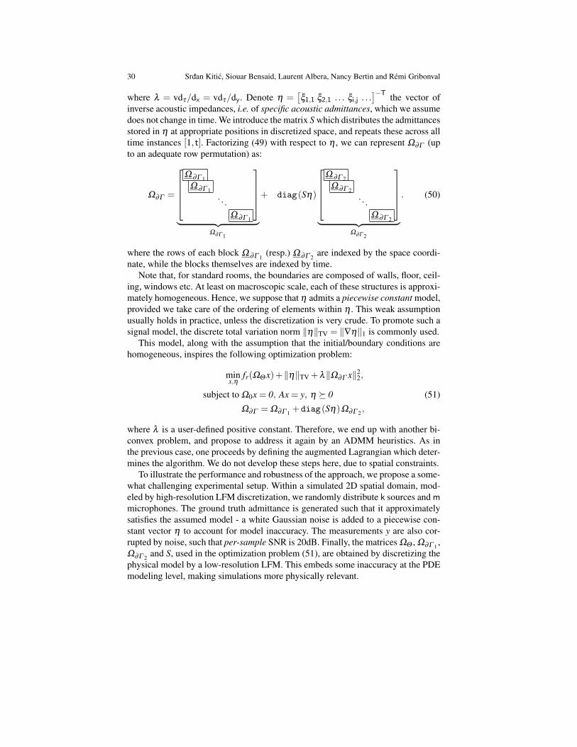
where λ = vdτ/dx = vdτ/dy. Denote η =[ξ1,1 ξ2,1 . . . ξi,j . . .
]−T the vector ofinverse acoustic impedances, i.e. of specific acoustic admittances, which we assumedoes not change in time. We introduce the matrix S which distributes the admittancesstored in η at appropriate positions in discretized space, and repeats these across alltime instances [1, t]. Factorizing (49) with respect to η , we can represent Ω∂Γ (upto an adequate row permutation) as:
Ω∂Γ =
Ω ∂Γ 1
Ω ∂Γ 1. . .
Ω ∂Γ 1
︸ ︷︷ ︸
Ω∂Γ 1
+ diag(Sη)
Ω ∂Γ 2
Ω ∂Γ 2. . .
Ω ∂Γ 2
︸ ︷︷ ︸
Ω∂Γ 2
. (50)
where the rows of each block Ω ∂Γ 1(resp.) Ω ∂Γ 2
are indexed by the space coordi-nate, while the blocks themselves are indexed by time.
Note that, for standard rooms, the boundaries are composed of walls, floor, ceil-ing, windows etc. At least on macroscopic scale, each of these structures is approxi-mately homogeneous. Hence, we suppose that η admits a piecewise constant model,provided we take care of the ordering of elements within η . This weak assumptionusually holds in practice, unless the discretization is very crude. To promote such asignal model, the discrete total variation norm ‖η‖TV = ‖∇η‖1 is commonly used.
This model, along with the assumption that the initial/boundary conditions arehomogeneous, inspires the following optimization problem:
minx,η
fr(ΩΘ x)+‖η‖TV +λ‖Ω∂Γ x‖22,
subject to Ω0x = 0, Ax = y, η 0 (51)Ω∂Γ = Ω∂Γ 1 +diag(Sη)Ω∂Γ 2 ,
where λ is a user-defined positive constant. Therefore, we end up with another bi-convex problem, and propose to address it again by an ADMM heuristics. As inthe previous case, one proceeds by defining the augmented Lagrangian which deter-mines the algorithm. We do not develop these steps here, due to spatial constraints.
To illustrate the performance and robustness of the approach, we propose a some-what challenging experimental setup. Within a simulated 2D spatial domain, mod-eled by high-resolution LFM discretization, we randomly distribute k sources and mmicrophones. The ground truth admittance is generated such that it approximatelysatisfies the assumed model - a white Gaussian noise is added to a piecewise con-stant vector η to account for model inaccuracy. The measurements y are also cor-rupted by noise, such that per-sample SNR is 20dB. Finally, the matrices ΩΘ , Ω∂Γ 1 ,Ω∂Γ 2 and S, used in the optimization problem (51), are obtained by discretizing thephysical model by a low-resolution LFM. This embeds some inaccuracy at the PDEmodeling level, making simulations more physically relevant.

Versatile and scalable cosparse methods for physics-driven inverse problems 31
The results in Figure 8 are with respect to average Euclidean distance betweenground truth source locations (empirical Root Mean Square Error (RMSE)), andthe estimated ones. The dashed line denotes the spatial step size of the coarse grid,thus the errors below this threshold are tolerated. The median RMSE values indicatethat localization is possible provided that the number of microphones is sufficientlyhigh. The error increases with the number of sources to localize, but usually remainslower than the double of spatial stepsize, suggesting that the sources are localizedin their true, immediate neighborhoods.
Fig. 8 RMSE for k= 1, k= 2 (top); and k= 3, k= 4 (bottom) simulated sources.
7.2 Cosparse brain source localization
Most source localization algorithms use one of the two following source models:the point source model, which explains the data with a small number of equivalentcurrent dipoles and the distributed source model, which uses thousands of dipoles.Whereas the latter allows for an estimation of the spatial extent of the source, itrequires to make assumptions about the spatial source distribution, which may leadto blurred (or even distorted) solutions [36]. On the other hand, the former oftengives helpful first approximations and superior performance in environments wherethere are few sources which are clustered [36]. Regarding head models, they aim atrepresenting geometrical and electrical properties of the different tissues composingthe volume conductor. Various models were proposed going from concentric ho-mogeneous spheres with isotropic conductivities for which analytic computationsof Green’s functions are possible, to realistically shaped models with refined tissueconductivity values [81].

32 Srdan Kitic, Siouar Bensaid, Laurent Albera, Nancy Bertin and Remi Gribonval
FEM discretization and head model. As seen in Section 4.2, FEM can be usedto discretize Poisson’s equation with Neumann boundary condition (9)-(10) and de-rive an equation of the form Ω x = c where the so-called linear analysis operator[60] Ω is the stiffness matrix, and vectors x and c respectively contain the potentialand total current flow values at the different nodes of the mesh. A realistic headmodel obtained from anatomical imaging modalities, such as Computed Tomogra-phy (CT) and structural Magnetic Resonance Imaging (sMRI), is segmented and alinear tetrahedral mesh of n nodes is then generated to divide it into small elementswhere a unique conductivity value is assigned to each one. In Figure 9, we illustratethe different steps performed to come to the sought algebraic system.
sMRI Segmentation Mesh
Fig. 9 The different steps of preprocessing in discretizing realistic head volume using FEM
As previously explained in section 4.2, the (n×n) matrix Ω is symmetric, pos-itive semidefinite, rank deficient by one and sparse with only few components ineach row [69]. Generally, instead of considering the singular linear system Ωx = c,another possibility is to transform it into a regular one and solve this instead. Theregular system is chosen such that its unique solution belongs to the set of solutionsof the original singular system. As described in [10], the easiest approach is to fixthe value of the potential to zero in one node. The special structure of the matrixΩ then allows us to cancel the corresponding row and column in Ω and also therespective entry in the right-hand side vector c. This leads to a system for which the(n−1×n−1) resulting matrix is symmetric, sparse and positive definite, as it canbe derived from a bilinear form satisfying the sames properties as a(., .) in section4.2. By abuse of notation we still denote it Ω . The solution of this system solves theinitial system with a zero potential value in the reference node.
Source model. We consider the following assumptions:
A1. There are g possible current sources that cover the volume of the gray matter G .A2. Each current source is modeled as a “pure” dipole, consisting in a point dipole
characterized by its position ρq and moment pq = ‖pq‖2 nq where ‖pq‖2 and nqcorrespond to the activity level and the orientation of the dipole, respectively. Inthis model, the current density is expressed as j = ∑
gq=1 pq δ (ρq) [71].

Versatile and scalable cosparse methods for physics-driven inverse problems 33
A3. Each current dipole is oriented orthogonally to the cortical surface (pq is thenormal to the cortical surface at position ρq).
A4. At most k (k<m) current dipoles have non-negligible activity.
In addition to the “pure” dipole, there are other numerical methods used to modelthe current dipole, such as the subtraction potential method and the direct potentialapproach using Saint Venant’s principle [83, 71]. Though the “pure” dipole is amathematical idealization of the real “physical” dipole that has finite current andseparation between its monopoles, it is frequently used for its simple derivation.
According to the variational form introduced in (15), the component ci in theload vector is
ci =∫
Θh
∇ · j φ i(r) dr. (52)
By applying Green’s identity to (52), using the fact that no current sources arepresent in the scalp ∂Θ , considering the expression of the domain Θh as a unionof d tetrahedra Θ e
h present in the mesh, and eventually assuming that each dipoleposition ρq coincides with a node position in G , appropriate calculations lead torewrite the entry in the load vector as:
ci =−pq · ∑e∈di ∇
eφ i(ρq) if ri = ρq
0 otherwise, (53)
where ∇eφ i is the gradient of function φ i over element Θ eh . By injecting the ex-
pression of dipole moment in (53) and in the case of non-zero ci, the latter can beexpressed as the product ci = ‖pq‖2 nq ·∑e∈di ∇
eφ i(ρq), which allows us to factorizevector c as c = Bz where B is a (n−1×n−1) diagonal matrix defined by
Bi,i =
−nq ·∑e∈di ∇
eφ i(ρq) if ri = ρq
1 otherwise. (54)
In addition, z is an (n− 1)-dimensional sparse vector with n− 1− g known zeroelements defined as
zi =‖pq‖2 if ri = ρq
0 otherwise. (55)
Consequently, matrix B conveys our knowledge about the orientation of the gdipoles of the grey matter G , while the non-zero elements in vector z represent theactivity of dipoles restricted to the cortical volume. It is noteworthy that, even whendipoles positions do not coincide with node positions, the factorization of vector cis still possible. However, in that case, the matrix B is no longer a square matrix butrather a tall matrix (not left invertible), which makes the computation of Ω morecomplicated. In addition, the assumption on the dipoles position is still realistic andaffordable by using a dense mesh in G .
Overall model. Combining the properties Ωx = c, the source model c = Bz andthe observation model y=Ax, the brain source localization defined above can finally

34 Srdan Kitic, Siouar Bensaid, Laurent Albera, Nancy Bertin and Remi Gribonval
be reformulated as a cosparse analysis model fitting problem given by:Ω x = zy = Ax,
(56)
where the analysis operator Ω is given by Ω = B−1 Ω and the sensing matrix A isan m×n−1 row-reduced identity matrix. As B is diagonal, Ω is still sparse.
Optimization problem. To address the cosparse analysis model fitting problem(56), we express the following convex optimization problem:
minv‖Ω1 x‖1 +λ‖Ω2 x‖2
2 (57)
subject to Ax = y.
where Ω1 is the (g× n− 1) submatrix of Ω obtained by extracting the rows of Ω
corresponding to the support set of the grey matter G , whereas Ω2 corresponds to therows indicated by the complementary set G . By choosing the appropriate weight λ ,the cosparse solution of the optimization problem (57) will fulfill the assumptions(A1) to (A4). Namely, ‖Ω1 x‖1 will promote sparsity at the surface of the cortex,while λ‖Ω2 x‖2
2 will attenuate the signal in the other regions. The linear constraintsAx = y ensure that the model fits the electrode measurements. Depending on theresolution of the cubic grid tuned by n, the problem can reach considerably largescale. Therefore, we use the Chambolle-Pock method as described in Section 5.2.
Experiments and performance criterion. One scenario was considered for acomparison of performance between the analysis and synthesis approaches. It aimsat studying the influence of the SNR.
More particularly, k = 2 synchronous epileptic dipoles were placed in G atρ1 = [−71,31,92]T and ρ2 = [−70,27,92]T, respectively, (locations are given incentimeters). Note that the origin (O) of the head model was defined as the intersec-tion of the O-Cz axis (z-axis), the O-T4 axis (x-axis) and the O-Fpz axis (y-axis).A physiologically-relevant model [40] was used to generate the time series corre-sponding to epileptic activity. It is noteworthy that this activity was the same forboth epileptic dipoles, leading to synchronous epileptic sources. On the other hand,the background activity, i.e. the activity of non-epileptic dipoles of G , was gener-ated as Gaussian and as temporally and spatially white. Its power was controlled bya multiplicative coefficient in order to get different SNR values.
As far as the head model is concerned, we used a realistic head model obtainedfrom sMRI. Ninety-one electrodes (m= 91) were placed on the scalp using the 10-5system [62]. In addition, in order to apply the FEM and compute the analysis opera-tor Ω , we created a linear tetrahedral mesh of n= 180585 nodes. Consequently, thesize of Ω and the number of dipoles of G were (n−1)×(n−1) = 180584×180584and g = 3110, respectively.
The quality of the source localization was quantified for each method by meansof the average Root Mean Square Error (RMSE), which is defined by:
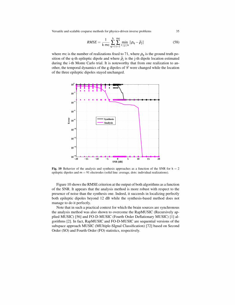
Versatile and scalable cosparse methods for physics-driven inverse problems 35
RMSE =1
k mc
k
∑q=1
mc
∑i=1
min1≤j≤k
‖ρq− ρj‖ (58)
where mc is the number of realizations fixed to 71, where ρq is the ground truth po-sition of the q-th epileptic dipole and where ρj is the j-th dipole location estimatedduring the i-th Monte Carlo trial. It is noteworthy that from one realization to an-other, the temporal dynamics of the g dipoles of G were changed while the locationof the three epileptic dipoles stayed unchanged.
−20 −15 −10 −5 0 5 10 15 2010−16
10−14
10−12
10−10
10−8
10−6
10−4
10−2
100
SNR [dB]
Err
or
SynthesisAnalysis
Fig. 10 Behavior of the analysis and synthesis approaches as a function of the SNR for k = 2epileptic dipoles and m= 91 electrodes (solid line: average, dots: individual realizations).
Figure 10 shows the RMSE criterion at the output of both algorithms as a functionof the SNR. It appears that the analysis method is more robust with respect to thepresence of noise than the synthesis one. Indeed, it succeeds in localizing perfectlyboth epileptic dipoles beyond 12 dB while the synthesis-based method does notmanage to do it perfectly.
Note that in such a practical context for which the brain sources are synchronousthe analysis method was also shown to overcome the RapMUSIC (Recursively ap-plied MUSIC) [56] and FO-D-MUSIC (Fourth Order Deflationary MUSIC) [1] al-gorithms [2]. In fact, RapMUSIC and FO-D-MUSIC are sequential versions of thesubspace approach MUSIC (MUltiple-SIgnal Classification) [72] based on SecondOrder (SO) and Fourth Order (FO) statistics, respectively.

36 Srdan Kitic, Siouar Bensaid, Laurent Albera, Nancy Bertin and Remi Gribonval
8 Summary and conclusion
In many physics-driven inverse problems, one can leverage both a sparsity hypoth-esis on some source term and the properties of the underlying PDE. A classical ap-proach to combine these ingredients is to build a dictionary of Green’s function ofthe PDE and to exploit traditional techniques (`1 regularization) for sparse synthe-sis reconstruction to estimate the source field. Yet, for high spatial and/or temporalresolutions, pre-computing Green’s functions can be challenging, and the synthesisversion of the `1 optimization problem may become numerically intractable due topolynomial complexities of too high degree in the overall size of the discretization.
An alternative is to discretize the PDE itself, e.g. through a Finite DifferenceScheme or the Finite Element Methods, which naturally leads to very sparse anal-ysis operators rather than dictionaries. While the two approaches (synthesis andanalysis) are formally equivalent, a primary advantage of the cosparse analysis reg-ularization is a much smaller iteration cost. Although demonstration of the full po-tential of the existing cosparse approaches on real acoustic or EEG data remainsto be done, results shown on simulated data allow to support our claims on theirinterest. Overall, as illustrated in this chapter, a promising approach to achieve pre-cision and scalability is to combine the synthesis approach and the analysis one in amultiscale optimization strategy. Besides scalability, the cosparse analysis approachopens interesting perspectives regarding the ability to solve extended inverse prob-lems where some physical parameters such as impedance or speed of sound maybe unknown. Using FEM, it allows to handle complex geometries, and as demon-strated on some brain source localization problems, it offers competitive robustnessto noise.
Beyond model-based methods, an intensive research in machine learning has re-cently inspired several training-based approaches, e.g. [43, 21, 3], which, however,either focus on a specific aspect of the problem at hand, or even neglect its explicitphysical nature. Instead, we feel that a promising research avenue are pre-trainedphysics-driven cosparse models, potentially leading to “fully-learnable” methods,unrestricted by parameterization or the geometry of the environment.
References
1. L. Albera, A. Ferreol, D. Cosandier-Rimele, I. Merlet, and F. Wendling. Brain source local-ization using a fourth-order deflation scheme. IEEE Transactions Biomedical Engineering,55(2):490–501, Feb. 2008.
2. L. Albera, S. Kitic, N. Bertin, G. Puy, and R. Gribonval. Brain source localization using aphysics-driven structured cosparse representation of eeg signals. In 2014 IEEE InternationalWorkshop on Machine Learning for Signal Processing (MLSP), September 21-24 2014.
3. N. Antonello, T. van Waterschoot, M. Moonen, and P. A. Naylor. Identification of surfaceacoustic impedances in a reverberant room using the FDTD method. In Acoustic Signal En-hancement (IWAENC), 2014 14th International Workshop on, pages 114–118. IEEE, 2014.
Versatile and scalable cosparse methods for physics-driven inverse problems 37
4. J. Barker, R. Marxer, E. Vincent, and S. Watanabe. The third chime speech separation andrecognition challenge: Dataset, task and baselines. In 2015 IEEE Workshop on AutomaticSpeech Recognition and Understanding (ASRU), pages 504–511, Dec 2015.
5. A. Beck and M. Teboulle. A fast iterative shrinkage-thresholding algorithm for linear inverseproblems. SIAM journal on imaging sciences, 2(1):183–202, 2009.
6. N. Bertin, S. Kitic, and R. Gribonval. Joint estimation of sound source location and boundaryimpedance with physics-driven cosparse regularization. In Acoustics, Speech and Signal Pro-cessing (ICASSP), 2016 IEEE International Conference on, pages 6340–6344. IEEE, 2016.
7. C. Bilen, S. Kitic, N. Bertin, and R. Gribonval. Sparse acoustic source localization withblind calibration for unknown medium characteristics. In iTwist-2nd international-TravelingWorkshop on Interactions between Sparse models and Technology, 2014.
8. C. Blandin, A. Ozerov, and E. Vincent. Multi-source TDOA estimation in reverberant audiousing angular spectra and clustering. Signal Processing, 92(8):1950–1960, 2012.
9. T. Blumensath and M. E. Davies. Sampling theorems for signals from the union of finite-dimensional linear subspaces. IEEE Transactions on Information Theory, 55(4):1872–1882,2009.
10. P. Bochev and R. B. Lehoucq. On the finite element solution of the pure Neumann problem.SIAM Review, 47(1):50–66, 2005.
11. S. Boyd, N. Parikh, E. Chu, B. Peleato, and J. Eckstein. Distributed optimization and statisticallearning via the alternating direction method of multipliers. Foundations and Trends R© inMachine Learning, 3(1):1–122, 2011.
12. J. Campbell. Introduction to Remote Sensing. Guilford Press, 1996.13. E. J. Candes, J. K. Romberg, and T. Tao. Stable signal recovery from incomplete and inac-
curate measurements. Communications on pure and applied mathematics, 59(8):1207–1223,2006.
14. A. Chambolle and T. Pock. A first-order primal-dual algorithm for convex problems withapplications to imaging. Journal of Mathematical Imaging and Vision, 40(1):120–145, 2011.
15. A. Chambolle and T. Pock. An introduction to continuous optimization for imaging. ActaNumerica, 25:161–319, 2016.
16. V. Chandrasekaran and M. I. Jordan. Computational and statistical tradeoffs via convex relax-ation. Proceedings of the National Academy of Sciences, 110(13):E1181–E1190, 2013.
17. G. Chardon, T. Nowakowski, J. De Rosny, and L. Daudet. A blind dereverberation method fornarrowband source localization. Journal of Selected Topics in Signal Processing, 2015.
18. P. L. Combettes and J.-C. Pesquet. Proximal splitting methods in signal processing. In Fixed-point algorithms for inverse problems in science and engineering, pages 185–212. Springer,2011.
19. L. Condat. A primal–dual splitting method for convex optimization involving lipschitzian,proximable and linear composite terms. Journal of Optimization Theory and Applications,158(2):460–479, 2013.
20. G. Dassios and A. Fokas. The definite non-uniqueness results for deterministic eeg and megdata. Inverse Problems, 29(6):065012, 2013.
21. A. Deleforge, F. Forbes, and R. Horaud. Acoustic space learning for sound-source sep-aration and localization on binaural manifolds. International journal of neural systems,25(01):1440003, 2015.
22. W. Deng and W. Yin. On the global and linear convergence of the generalized alternatingdirection method of multipliers. Journal of Scientific Computing, 66(3):889–916, 2016.
23. A. Devaney and G. Sherman. Nonuniqueness in inverse source and scattering problems. IEEETransactions on Antennas and Propagation, 30(5):1034–1037, 1982.
24. I. Dokmanic. Listening to Distances and Hearing Shapes. PhD thesis, EPFL, 2015.25. I. Dokmanic and M. Vetterli. Room helps: Acoustic localization with finite elements. In IEEE
International Conference on Acoustics, Speech and Signal Processing (ICASSP), 2012, pages2617–2620. Ieee, 2012.
26. P. L. Dragotti, M. Vetterli, and T. Blu. Sampling moments and reconstructing signals of fi-nite rate of innovation: Shannon meets strang–fix. IEEE Transactions on Signal Processing,55(5):1741–1757, 2007.
38 Srdan Kitic, Siouar Bensaid, Laurent Albera, Nancy Bertin and Remi Gribonval
27. J. Eckstein and D. P. Bertsekas. On the Douglas-Rachford splitting method and the proximalpoint algorithm for maximal monotone operators. Mathematical Programming, 55(1):293–318, 1992.
28. M. Elad, P. Milanfar, and R. Rubinstein. Analysis versus synthesis in signal priors. Inverseproblems, 23(3):947, 2007.
29. D. C.-L. Fong and M. Saunders. LSMR: An iterative algorithm for sparse least-squares prob-lems. SIAM Journal on Scientific Computing, 33(5):2950–2971, 2011.
30. I. Fried. Bounds on the spectral and maximum norms of the finite element stiffness, flexibilityand mass matrices. International Journal of Solids and Structures, 9(9):1013–1034, 1973.
31. A. Friedman. Partial differential equations of parabolic type. Courier Dover Publications,2008.
32. D. Gabay and B. Mercier. A dual algorithm for the solution of nonlinear variational problemsvia finite element approximation. Computers & Mathematics with Applications, 2(1):17–40,1976.
33. S. Gannot, D. Burshtein, and E. Weinstein. Signal enhancement using beamforming and non-stationarity with applications to speech. IEEE Transactions on Signal Processing, 49(8):1614–1626, 2001.
34. M. S. Gockenbach. Understanding and implementing the finite element method. SIAM, 2006.35. T. Goldstein, B. O’Donoghue, S. Setzer, and R. Baraniuk. Fast alternating direction optimiza-
tion methods. SIAM Journal on Imaging Sciences, 7(3):1588–1623, 2014.36. R. Grech, T. Cassar, J. Muscat, K. P. Camilleri, S. G. Fabri, M. Zervakis, P. Xanthopoulos,
V. Sakkalis, and B. Vanrumste. Review on solving the inverse problem in EEG source analysis.Journal of NeuroEngineering and Rehabilitation, 7:5–25, November 2008.
37. H. Hallez, B. Vanrumste, R. Grech, J. Muscat, W. De Clercq, A. Vergult, Y. D ’asseler, K. P.Camilleri, S. G. Fabri, S. V. Huffel, and I. Lemahieu. Review on solving the forward problemin EEG source analysis. J. Neuroeng. Rehabil., 4(4), 2007.
38. M. Herman, T. Strohmer, et al. General deviants: An analysis of perturbations in compressedsensing. IEEE Journal of Selected topics in signal processing, 4(2):342–349, 2010.
39. V. Isakov. Inverse problems for partial differential equations, volume 127. Springer Science& Business Media, 2006.
40. B. H. Jansen and V. G. Rit. Electroencephalogram and visual evoked potential generation ina mathematical model of coupled cortical columns? Biological Cybernetics, 73(4):357–366,Sept. 1995.
41. R. Jenatton, J.-Y. Audibert, and F. Bach. Structured variable selection with sparsity-inducingnorms. The Journal of Machine Learning Research, 12:2777–2824, 2011.
42. C. R. Johnson. Computational and numerical methods for bioelectric field problems. Crit.Rev. Biomed. Eng., 25(1):1–81, 1997.
43. U. S. Kamilov and H. Mansour. Learning optimal nonlinearities for iterative thresholdingalgorithms. IEEE Signal Processing Letters, 23(5):747–751, 2016.
44. Y. Kim and P. Nelson. Optimal regularisation for acoustic source reconstruction by inversemethods. Journal of Sound and Vibration, 275(35):463 – 487, 2004.
45. S. Kitic, L. Albera, N. Bertin, and R. Gribonval. Physics-driven inverse problems madetractable with cosparse regularization. IEEE Transactions on Signal Processing, 64(2):335–348, 2016.
46. S. Kitic, N. Bertin, and R. Gribonval. Hearing behind walls: localizing sources in the roomnext door with cosparsity. In Acoustics, Speech and Signal Processing (ICASSP), 2014 IEEEInternational Conference on, pages 3087–3091. IEEE, 2014.
47. K. Kowalczyk and M. v. Walstijn. Modeling frequency-dependent boundaries as digitalimpedance filters in FDTD and K-DWM room acoustics simulations. Journal of the AudioEngineering Society, 56(7/8):569–583, 2008.
48. H. Kuttruff. Room acoustics. Crc Press, 2016.49. J. Le Roux, P. T. Boufounos, K. Kang, and J. R. Hershey. Source localization in reverberant
environments using sparse optimization. In IEEE International Conference on Acoustics,Speech and Signal Processing (ICASSP), 2013, pages 4310–4314. IEEE, 2013.

Versatile and scalable cosparse methods for physics-driven inverse problems 39
50. R. J. LeVeque. Finite difference methods for ordinary and partial differential equations:steady-state and time-dependent problems. SIAM, 2007.
51. T. T. Lin and F. J. Herrmann. Compressed wavefield extrapolation. Geophysics, 72(5):SM77–SM93, 2007.
52. D. Malioutov. A sparse signal reconstruction perspective for source localization with sensorarrays, master’s thesis, 2003.
53. D. Malioutov, M. Cetin, and A. S. Willsky. A sparse signal reconstruction perspective forsource localization with sensor arrays. IEEE Transactions on Signal Processing, 53(8):3010–3022, 2005.
54. M. Mohr and B. Vanrumste. Comparing iterative solvers for linear systems associated withthe finite difference discretisation of the forward problem in electro-encephalographic sourceanalysis. Medical and Biological Engineering and Computing, 41:75–84, 2003.
55. J.-J. Moreau. Proximite et dualite dans un espace hilbertien. Bulletin de la Societemathematique de France, 93:273–299, 1965.
56. J. C. Mosher and R. M. Leahy. Source localization using Recursively Applied and Projected(RAP) music. IEEE Transactions On Signal Processing, 47(2):332–340, Feb. 1999.
57. W. Munk, P. Worcester, and C. Wunsch. Ocean acoustic tomography. Cambridge UniversityPress, 2009.
58. G. Mur. Absorbing boundary conditions for the finite-difference approximation of the time-domain electromagnetic-field equations. IEEE transactions on Electromagnetic Compatibil-ity, EMC-23(4):377–382, 1981.
59. J. Murray-Bruce and P. L. Dragotti. Solving physics-driven inverse problems via structuredleast squares. In Signal Processing Conference (EUSIPCO), 2016 24th European, pages 331–335. IEEE, 2016.
60. S. Nam, M. E. Davies, M. Elad, and R. Gribonval. The cosparse analysis model and algo-rithms. Applied and Computational Harmonic Analysis, 34(1):30–56, January 2013.
61. Y. Nesterov. Introductory lectures on convex optimization: A basic course, volume 87.Springer Science & Business Media, 2013.
62. R. Oostenvelda and P. Praamstra. The five percent electrode system for high-resolution EEGand ERP measurements. Clinical Neurophysiology, Elsevier, 112(4):713–719, April 2001.
63. A. Pezeshki, Y. Chi, L. L. Scharf, and E. K. Chong. Compressed sensing, sparse inversion,and model mismatch. In Compressed Sensing and its Applications, pages 75–95. Springer,2015.
64. T. Piotrowski, D. Gutierrez, I. Yamada, and J. Zygierewicz. Reduced-rank neural activity indexfor EEG/MEG multi-source localization. In ICASSP’14, IEEE International Conference onAcoustics Speech and Signal Processing, Florence, Italy, May 4-9 2014.
65. L. C. Potter, E. Ertin, J. T. Parker, and M. Cetin. Sparsity and compressed sensing in radarimaging. Proceedings of the IEEE, 98(6):1006–1020, 2010.
66. J. Provost and F. Lesage. The application of compressed sensing for photo-acoustic tomogra-phy. IEEE transactions on medical imaging, 28(4):585–594, 2009.
67. Qianqian Fang and D. A. Boas. Tetrahedral mesh generation from volumetric binary andgrayscale images. In 2009 IEEE Int. Symp. Biomed. Imaging From Nano to Macro, pages1142–1145. IEEE, jun 2009.
68. A. Rosenthal, D. Razansky, and V. Ntziachristos. Fast semi-analytical model-based acousticinversion for quantitative optoacoustic tomography. IEEE transactions on medical imaging,29(6):1275–1285, 2010.
69. Y. Saad. Iterative methods for sparse linear systems. SIAM, 2003.70. O. Scherzer, M. Grasmair, H. Grossauer, M. Haltmeier, and F. Lenzen. Variational methods
in imaging, volume 320. Springer, 2009.71. P. Schimpf, C. Ramon, and J. Haueisen. Dipole models for the EEG and MEG. IEEE Trans.
Biomed. Eng., 49(5):409–418, may 2002.72. R. Schmidt. Multiple emitter location and signal parameter estimation. IEEE Transactions On
Antennas Propagation, 34(3):276–280, Mar. 1986. Reprint of the original 1979 paper fromthe RADC Spectrum Estimation Workshop.

40 Srdan Kitic, Siouar Bensaid, Laurent Albera, Nancy Bertin and Remi Gribonval
73. S. Shalev-Shwartz and N. Srebro. SVM optimization: inverse dependence on training set size.In Proceedings of the 25th international conference on Machine learning, pages 928–935.ACM, 2008.
74. R. Shefi and M. Teboulle. Rate of convergence analysis of decomposition methods based onthe proximal method of multipliers for convex minimization. SIAM Journal on Optimization,24(1):269–297, 2014.
75. J.-L. Starck and J. M. Fadili. An overview of inverse problem regularization using sparsity. InIEEE ICIP, pages 1453 – 1456, Cairo, Egypt, Nov. 2009.
76. G. Strang. Computational science and engineering, volume 791. Wellesley-Cambridge PressWellesley, 2007.
77. L. Thomas. Using a computer to solve problems in physics. Applications of digital computers,pages 44–45, 1963.
78. J. A. Tropp and S. J. Wright. Computational methods for sparse solution of linear inverseproblems. Proceedings of the IEEE, 98(6):948–958, June 2010.
79. K. Uutela, M. Hamalainen, and E. Somersalo. Visualization of magnetoencephalographic datausing minimum current estimates. Elsevier NeuroImage, 10(2):173–180, August 1999.
80. J.-M. Valin, F. Michaud, J. Rouat, and D. Letourneau. Robust sound source localization usinga microphone array on a mobile robot. In Proceedings. 2003 IEEE/RSJ International Con-ference on Intelligent Robots and Systems, 2003.(IROS 2003)., volume 2, pages 1228–1233.IEEE, 2003.
81. F. Vatta, F. Meneghini, F. Esposito, S. Mininel, and F. Di Salle. Realistic and spherical headmodeling for EEG forward problem solution: A comparative cortex-based analysis. Compu-tational Intelligence and Neuroscience, 2010.
82. M. Vetterli, P. Marziliano, and T. Blu. Sampling signals with finite rate of innovation. IEEEtransactions on Signal Processing, 50(6):1417–1428, 2002.
83. C. Wolters, H. Kostler, C. Moller, J. Hardtlein, and A. Anwander. Numerical approachesfor dipole modeling in finite element method based source analysis. International CongressSeries, 1300:189 – 192, 2007.