Verifying single-station seismic approaches using

Earth-based data: Preparation for data return from the

InSight mission to Mars

Mark P. Panninga, Eric Beuclerb, Melanie Drilleaub,c, Antoine Mocquetb,Philippe Lognonnec, W. Bruce Banerdtd

aDepartment of Geological Sciences, University of FloridabLaboratoire de Planetologie et Geodynamique, Universite de Nantes

cUniv Paris Diderot-Sorbonne Paris Cite, Institut de Physique du Globe ParisdJet Propulsion Laboratory, California Institute of Technology

Abstract

The planned InSight mission will deliver a single seismic station containing3-component broadband and short-period sensors to the surface of Mars in2016. While much of the progress in understanding the Earth and Moon’sinterior has relied on the use of seismic networks for accurate location ofsources, single station approaches can be applied to data returned from Marsin order to locate events and determine interior structure. In preparation forthe data return from InSight, we use a terrestrial dataset recorded at theGlobal Seismic Network station BFO, located at the Black Forest Obser-vatory in Germany, to verify an approach for event location and structuredetermination based on recordings of multiple orbit surface waves, which willbe more favorable to record on Mars than Earth due to smaller planetary ra-dius and potentially lower background noise. With this approach applied toevents near the threshold of observability on Earth, we are able to determineepicentral distance within approximately 1 degree (corresponding to ∼60 kmon Mars), and origin time within ∼30 seconds. With back azimuth deter-mined from Rayleigh wave polarization, absolute locations are determinedgenerally within an aperture of 10 degrees, allowing for localization withinlarge tectonic regions on Mars. With these locations, we are able to recoverEarth mantle structure within ±5% (the InSight mission requirements forMartian mantle structure) using 1D travel time inversions of P and S traveltimes for datasets of only 7 events. The location algorithm also allows forthe measurement of great-circle averaged group velocity dispersion, which we

Preprint submitted to Icarus October 14, 2014

measure between 40 and 200 seconds to scale the expected reliable frequencyrange of the Insight data from Earth to Mars data. Using the terrestrialdata, we are able to resolve structure down to ∼200 km, but synthetic testsdemonstrate we should be able to resolve Martian structure to ∼400 km withthe same frequency content given the smaller planetary size.

Key words: Mars, interior, Geophysics, Earth

1. Introduction

Seismology is one of the strongest observational tools available in orderto constrain the deep interior structure of planetary bodies (Lognonne andJohnson, 2007). After the advent of quality seismometers in the late 19thand early 20th centuries, our knowledge of Earth structure expanded rapidlywith the discovery of the core by Richard Oldham in 1906, the crust-mantlediscontinuity by Andrija Mohorovicic in 1909, and the inner core by IngeLehmann in 1936. By 1939, Harold Jeffreys had produced a 1D global modelof the whole Earth capable of matching P wave arrivals within 0.2% (see e.g.Lay and Wallace, 1995, ch. 1). In addition to the Earth, however, we haveretrieved instrumental seismic data with clear evidence of interior signalsonly from the Earth’s moon. The data from seismometers deployed on theMoon as part of Apollo Passive Seismic Experiment by astronauts in four ofthe six Apollo missions between 1969 and 1972, which recorded data until1977, gave first order constraints on lunar structure, while also producingvery unexpected seismograms showing high levels of scattering (e.g. Naka-mura, 1983). While we have not received any more data from the Moonsince the 1970’s, recent research applying more more advanced seismologi-cal approaches developed since the initial studies have refined this model,and revealed more information about possible core layering and partial melt-ing (Khan and Mosegaard, 2002; Lognonne et al., 2003; Chenet et al., 2006;Gagnepain-Beyneix et al., 2006; Khan et al., 2007; Garcia et al., 2011; Weberet al., 2011).

The power of seismology to illuminate planetary interiors is one of theprimary motivations behind the planned InSight lander mission to Mars(Banerdt et al., 2013), which will include 3-component broadband and shortperiod seismometers (SEIS experiment, (Lognonne et al., 2012a; Mimounet al., 2012)), as well as a heat flow probe (HP3), a geodetic experiment(RISE), and a magnetometer, in addition to meteorological sensors. While

2

2 seismometers, with sensitivity limited to 1 to 5 orders of magnitude lowerthan that of the Apollo seismometers, were landed on Mars during the Vikingmissions in the late 1970’s, the seismometer on Viking 1 did not properlyuncage, and the placement of the seismometer on the top of the Viking 2lander prevented the recovery of any signals definitively originating in theplanetary interior, although one possible internal signal was identified (An-derson et al., 1977). 20 years later, the second attempt with the OPTIMISMseismometers (Lognonne et al., 1998) onboard two Small Autonomous Sta-tions (Linkin et al., 1998) was lost due to a Mars 96 mission launch stagefailure. While the seismometer from the Viking mission did give us a solidupper bound on the Martian seismicity level and may have observed an inter-nal event, the higher sensitivity of the InSight seismometer installation (bothdue to instrument sensitivity and installation on the surface of Mars ratherthan atop a lander), greatly enhances our capability of observing Martianseismicity. Despite the lack of seismic observational data to date, basic con-straints from planetary mass and moment of inertia and some assumptionson bulk chemistry based on constraints primarily from SNC meteorites (Mc-Sween, 1994) have allowed for several estimates of the internal elastic andcompositional structure of Mars (e.g. Mocquet et al., 1996; Sohl and Spohn,1997; Gudkova and Zharkov, 2004; Rivoldini et al., 2011).

Many of the advances of Earth seismology have been built on the conceptof networks of multiple instruments, which allow for accurate determinationof source parameters for recorded quakes, and the four instruments of theApollo Passive Seismic Experiment built on this legacy for planetary seismol-ogy. Logically, proposals for Martian seismometry, such as the NetLandermission (Lognonne et al., 2000; Dehant et al., 2004), have also attempted toset up networks using multiple landers. Multiple landers with geophysicalinstruments, however, lead to large expenses, and for this reason, the Insightmission has chosen to focus on a single lander and seismic station deployment,requiring a different strategy than simple body wave travel times inversionfor the determination of the interior structure. While most of Earth seismol-ogy does rely on networks and the accurate locations they allow, there aremany techniques that can be applied to single station data, including receiverfunctions (e.g. Phinney, 1964; Vinnik et al., 2001) and normal mode analy-sis (e.g. Lognonne et al., 1998). We focus on the ability of a single stationapproach like that of InSight to achieve the science goal of resolving man-tle velocity structure within ±5%, which will give us strong constraints onthe internal structure and evolution of another terrestrial planet for the first

3

time. In this study, we verify the potential of single-station data using loca-tions determined from multiple orbit surface waves both for determination oftectonically active regions as well as allowing for travel time inversions for 1Dmantle velocity structure. Surface wave dispersion analysis is also possiblewith single station data, and we show that we should be able to resolve uppermantle velocity structure with group velocity dispersion measurements madeat a single station using multiple orbit surface waves.

2. Expected Martian seismicity

Given the lack of direct observations of seismic activity from the Vikinglanders compared to the installation and instrument noise observed in thatexperiment (Anderson et al., 1977), we are able to constrain a rough upperbound on seismicity (based on the lack of observations) roughly equivalent tointraplate activity on Earth (Solomon et al., 1991). The Earth’s intraplateactivity level (the number of events per year of a given seismic moment) isshown by the solid red line on fig. 1. On the other hand, we would expectthere to be a higher rate of cooling on Mars than on the Moon, and wouldtherefore expect seismicity rates due to thermal contraction to be higherthan lunar rates (e.g. Solomon et al., 1991; Phillips, 1991; Knapmeyer et al.,2006, see red line with triangles on fig. 1). Constraining the seismic activityof Mars, therefore, will obviously be a first order result from the proposedInSight mission.

Seismicity levels can also be estimated in advance of instrumental databy using thermal modeling (Phillips, 1991) or analysis of surface faulting(Golombek et al., 1992; Golombek, 2002; Knapmeyer et al., 2006) (fig. 1).While there is certainly a large amount of uncertainty in these estimates,most values cluster in a range which implies we potentially may observe 1-10 events with seismic moment near 1017 Nm (moment magnitude MW5.3)during the nominal Martian year duration of the mission. Excitation ofnormal modes above the observational limit ( about 10−9 ms−2/Hz1/2 ) islikely for moment larger than 1017 Nm and will then allow inversions of thenormal modes eigenfrequencies between 50 sec and 100 sec (Lognonne et al.,1996). We however do not discuss here such inversion, but instead focus onsmaller quakes, expected to occur at a higher rate and therefore possibly stillobservable even in the case of a weaker than expected seismicity of Mars.

Events near the range of 1016 to 1017 Nm in moment release are impor-tant as they will likely be large enough to observe multiple orbit surface

4

waves (i.e. surface waves that either travel on the major arc to the stationor have at least one full great-circle transit of the planet). When recordedon a quiet station on Earth, these multiple orbit surface waves begin to be-come reliably observable for events with a moment of ∼1018 Nm (MW 6).These low amplitudes are mainly related to attenuation effects: Rayleighsurface waves at 100 sec have group velocity of about 3.8 km/s and a qualityfactor of Q = 120, so the attenuation factor (αEarth =exp(− ωt

2Q) ) after one

circuit around the planet (about 3 hr) is about 1/15. Even if the mantleattenuation of Mars is relatively high (i.e. relatively low Q), the Martianthermal lithosphere (which on Earth has relatively low attenuation) is ex-pected to be much thicker and the attenuation of such a surface wave, whichhas peak energy at a depth of 100-200 km, is therefore expected to be muchless than on Earth (Lognonne and Mosser, 1993; Nimmo and Faul, 2013).The corresponding Martian attenuation factor is therefore expected to be

αMars = α

[aMars×QEarthaEarth×QMars

]Earth , (1)

where aEarth and aMars are the radii of Earth and Mars, respectively. Both thesmaller radius and the expected larger QMars makes the attenuation factormuch smaller on Mars. Even if we assume identical Q on Mars to Earth,multiple orbit surface waves will have amplitudes that are larger roughly byan order of magnitude simply due to the smaller planetary radius(fig. 2).The likely higher Q on Mars due to the expected thicker thermal lithospherewould only enhance this effect. For this reason, it is reasonable to expectthat multiple orbit surface waves will likely be observable for events withmoments ranging from 1016 Nm to 1017 Nm.

3. Surface wave-based single station location

In order to use surface waves for location, we need to be able to recordmultiple orbit surface waves. At a minimum, we need to be able to mea-sure timing of the minor and major arc, plus the third orbit (minor arc plusanother trip around the great circle path). We break the location probleminto two parts. First, we determine distance and origin time from the tim-ing of the first three orbits. This should be a relatively robust approach,as it relies only on the vertical component, which is likely to be the leastnoisy component of data recovered. This determination alone is sufficient forusing body wave travel times to perform inversions for spherically averaged

5

10−4

10−2

100

102

104

106

1010 1012 1014 1016 1018 1020 1022

10−4

10−2

100

102

104

106

1010 1012 1014 1016 1018 1020 1022

10−4

10−2

100

102

104

106

1010 1012 1014 1016 1018 1020 1022

10−4

10−2

100

102

104

106

1010 1012 1014 1016 1018 1020 1022

10−4

10−2

100

102

104

106

1010 1012 1014 1016 1018 1020 1022

10−4

10−2

100

102

104

106

1010 1012 1014 1016 1018 1020 1022

10−4

10−2

100

102

104

106

1010 1012 1014 1016 1018 1020 1022

10−4

10−2

100

102

104

106

1010 1012 1014 1016 1018 1020 1022

10−4

10−2

100

102

104

106

1010 1012 1014 1016 1018 1020 1022

10−4

10−2

100

102

104

106

1010 1012 1014 1016 1018 1020 1022

10−4

10−2

100

102

104

106

1010 1012 1014 1016 1018 1020 1022

10−4

10−2

100

102

104

106

1010 1012 1014 1016 1018 1020 1022

10−4

10−2

100

102

104

106

1010 1012 1014 1016 1018 1020 1022

10−4

10−2

100

102

104

106

1010 1012 1014 1016 1018 1020 1022

Phillips (1991)

Golombek et al. (1992)

Golombek (2002)

Knapmeyer et al. (2006)

Lunar

Earth

Earth intraplate

Seismic Moment M0 [Nm]

N(M

>=

M0)/

yr

Figure 1: Estimates of Martian seismicity plotted as the number of events per Earthyear greater than a given seismic moment vs. moment. Earth activity line is derivedfrom a fit to the linear portion of the Harvard CMT catalog from 1984-2004 (Dziewonskiand Woodhouse, 1983), while the intraplate line is simply 0.5% of the full Earth momentrelease based on studies of continental intraplate seismicity (Johnson and Kanter, 1990;Okal and Sweet, 2007). The lunar activity line is derived from the catalog of Nakamuraet al. (1979). The dashed horizontal line represents the level above which we would expectto see a few events during the InSight mission, while the vertical dash-dot lines at 1016

and 1018 Nm represent the moment range over which we would expect 3rd orbit Rayleighwaves to become observable. Figure adapted from Knapmeyer et al. (2006).

6

0,01

0,1

1

10

0 1250 2500 3750 5000 6250 7500 8750 10000

Epicentral Distance, km

R1 Mars

R1 Earth

R2 Mars

R3 Mars

R2 Earth

R3 Earth

50 s period

Relative amplitude

Figure 2: Amplitude of Rayleigh wave trains with a period of 50 s normalized by R1 (minorarc) amplitude at an epicentral distance of 10,000 km on Earth. Calculations are madeassuming identical spatial Q of 150, and only taking into account differences in geometricalspreading and propagation distance. Note that R2 and R3 on Mars are larger than onEarth by roughly an order of magnitude.

structure. Next, we determine back azimuth using rotation of the horizontalcomponents. Of course, this measurement may be more problematic withdata from the single seismic station of the InSight mission, but we demon-strate that we can localize events within large tectonic regions if we do havehorizontal measurements of sufficient quality.

3.1. Distance and origin time

If we are able to record up to 3rd orbit surface waves, determining distanceand origin time of the source is a straightforward process. For this process,we filter the data in a series of frequency bands and take the envelope inorder to pick the maximum energies of the first three orbits of the Rayleighwave. Let us denote the arrival times at a given frequency band R1, R2, andR3. The angular group velocity is then

U =2π

R3−R1, (2)

where the angular distances are measured in radians, and angular groupvelocity is in radians/sec. These velocities can be converted to more typicalunits such as km/sec by multiplying by the planetary radius. The epicentraldistance, ∆, and origin time, t0, can then be derived as

∆ = π − 1

2U(R2−R1) (3)

7

t0 = R1− ∆

U. (4)

Of course, we could do a similar process for the Love waves, but noise isexpected to be lower on the vertical component (based on both experiencewith terrestrial seismic deployments and expectation of pressure-induced tiltnoise on the horizontal components in the surface wave frequency band), andthis will be the most robust means of estimating distance and origin time.

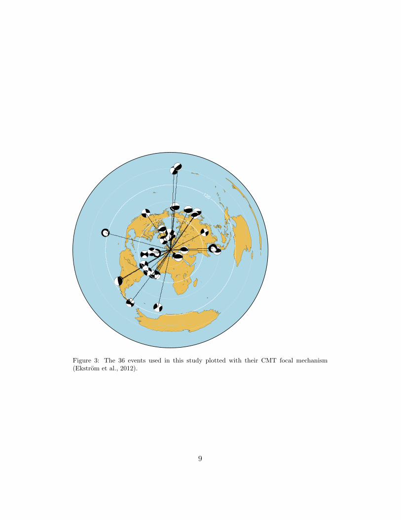
In order to verify this basic approach, and to determine the level of errorin location that can be expected with such a procedure, we collected datafrom 36 shallow events at a variety of epicentral distances in the magnituderange M6.0-M6.5 measured on the Global Seismic Network station BFO,located at the Black Forest Observatory in Germany (fig. 3). The eventlocations and CMT moment magnitudes (Ekstrom et al., 2012) are shownin table 1. Note that the initial data selection was based on a catalog ofbody wave (mb) magnitudes, and so a few of the CMT MW magnitudes areabove and below the original range (ranging from 5.68 to 6.88 in MW ). Theevents discussed in this paper were chosen primarily to get a relatively evendistribution of shallow events as a function of distance and then applying ourprocessing approach to the first few events in each distance range for whichwe were able to visually identify R2 and R3 arrivals in 100 second lowpassfiltered data. No further selection criteria were applied to the events toselect ”clean” data or advantageous focal mechanisms or to ensure azimuthaldistribution. Note that we limit ourselves to shallow events because deepevents do not excite fundamental mode surface waves efficiently. We filterthe data with a series of zero phase Butterworth bandpass filters, and takethe envelopes of the resulting seismograms (example shown in fig. 4). WhileR2 and R3 are typically not visually clear in the broadband time series data,these magnitudes are just large enough to allow the multiple orbit surfacewaves to emerge above the noise in some frequency bands, permitting us toassess how well such a method will perform if multiple orbit surface waves areobservable for events recorded on Mars. We used an automated algorithmto select R1, R2, and R3 arrival times by picking peak energy values as afunction of frequency. For each frequency band, we obtain an independentestimate of epicentral distance, ∆, and origin time, t0, as well as groupvelocity, U as a function of frequency (which is used in section 5 to invertfor upper mantle velocity structure). Using multiple frequency bands allowsus to assess the consistency of the source parameter estimates and throw outinconsistent data.

8

60

120

Figure 3: The 36 events used in this study plotted with their CMT focal mechanism(Ekstrom et al., 2012).

9

Event Latitude Longitude Depth Mw Dist err (◦) t0 err (s)C200802201827A 36.24 21.73 17.6 6.16 -0.56 52.67C200802210246A 77.02 19.28 12.8 6.07 0.64 24.81C200805291546A 63.92 -21.17 12.0 6.29 -1.96 -61.53C200907010930A 34.00 25.50 12.0 6.45 -0.59 -13.65C200908200635A 72.22 0.84 12.0 5.99 0.21 11.09C200909072241A 42.61 43.51 13.4 5.98 -3.07 16.43C200704050356A 37.45 -24.44 12.0 6.34 0.06 0.56C200704070709A 37.40 -24.38 12.0 6.06 -0.24 -11.54C200903061050A 80.33 -2.32 13.0 6.47 -0.31 -7.35C200906062033A 23.94 -46.12 12.0 6.00 -0.38 -9.61C200907071911A 75.33 -72.49 16.5 6.03 -0.14 9.42C200912091600A -0.62 -20.80 26.5 6.41 -0.01 8.00C201005251009A 35.31 -35.80 15.5 6.30 0.42 19.60C200705041206A -1.12 -14.92 12.7 6.22 0.29 -4.11C200707030826A 0.81 -30.04 17.0 6.31 -0.34 1.55C200707312255A 0.04 -17.86 21.8 6.17 -0.22 -10.59C200708202242A 8.19 -39.17 12.0 6.54 0.63 5.95C200803030931A 46.26 153.38 13.6 6.48 0.96 14.92C200803151443A 2.47 94.51 12.0 6.03 -0.01 -28.15C200804160554A 51.81 -179.17 12.0 6.60 -0.51 -5.83C200805201353A 51.11 178.53 17.6 6.27 -0.34 9.45C200805250821A 32.57 105.45 27.0 6.07 0.36 -66.22C200806132343A 39.03 140.85 12.0 6.88 1.19 -17.84C200806271140A 10.92 91.82 17.1 6.57 0.74 -11.66C200806281254A 10.90 91.80 12.0 6.08 0.94 25.00C201001100027A 40.53 -124.81 19.0 6.51 1.08 -5.05C201003140808A 37.70 141.98 45.9 6.53 0.55 -65.16C201003300102A 43.28 138.45 12.0 5.75 0.82 -23.56C201001050455A -58.50 -14.85 15.1 6.77 -1.26 -20.95C201001171200A -57.94 -66.16 18.6 6.24 0.33 65.24C201002090103A -15.00 -173.07 15.0 6.05 -0.02 19.95C201002130234A -22.19 -174.06 20.0 6.03 -0.30 -22.85C201003070705A -16.34 -115.45 12.7 6.26 0.29 7.10C201003121650A -34.41 -72.18 12.0 5.68 0.39 -20.28C201003151108A -35.96 -73.85 12.0 6.19 0.03 -39.27C201003160221A -36.49 -73.63 13.4 6.64 0.48 -14.94

Table 1: Event CMT identifiers, latitude and longitude (in degrees) and depth (km) forthe dataset used in this study.

10

0

5000

10000

15000

Tim

e (s

)

0.0050.010.02

Frequency (Hz)

0.25 0.50 0.75normalized A

50 100 200

Period (s)

0

5000

10000

15000

Tim

e (s

)

BFO Z 2008 052

Figure 4: Example envelope processing for a magnitude 6.1 quake in Svalbard (eventC200802210246A in table 1) at a distance of 29.1◦ from BFO. Color scale is normalized topeak amplitude in each frequency band. R2 can be seen at longer periods arriving between10000 and 11000 s, and R3 between 12000 and 13000 s.

11

For our dataset of events recorded at BFO, we compared our estimatedepicentral distances and origin times with the catalog locations to estimatethe approximate error we can expect with such an approach on Martiandata (fig. 5). As shown in the histograms and table 1, most events arelocated within 1◦ for epicentral distance (which corresponds to about 60 kmon Mars) and 30 seconds in origin time, although a few outlying locations areincluded in the dataset. While these errors are clearly quite large in compar-ison with network-determined locations used in most terrestrial seismologyapplications, we are able to use them in combination with a small number ofpicked P and S arrival times (section 4) to invert for mantle velocity profilesthat meet InSight mission requirements.

0

2

4

6

8

Co

un

t

−3.0 −2.4 −1.8 −1.2 −0.6 0.0 0.6 1.2

Distance error (degrees)

A

−60 −40 −20 0 20 40 60

Origin time error (s)

B

Figure 5: Histograms of errors in epicentral distance (A) and origin time (B) estimatedfrom multiple orbit Rayleigh wave arrival times relative to catalog locations.

3.2. Back azimuth determination

While epicentral distance and origin time are adequate for the inversionof travel times for 1D velocity structure, we also need back azimuth in orderto localize any recorded events to a particular tectonic region on Mars. Whilemost event location schemes on the Earth rely on travel times recorded ina network of stations, it is possible to determine the back azimuth basedon the polarization of particular seismic phases recorded on 3-componentseismograms. For example, any P-SV phases will be polarized in the great-circle plane containing the source and receiver, and can be used to determineback-azimuth. For this study, we are focusing on the utility of the longerperiod surface wave data, and the known elliptical particle motion of Rayleigh

12

waves has been utilized in the past for single station location in the contextof nuclear monitoring on Earth (e.g. Chael, 1997; Baker and Stevens, 2004).Any such polarization approach relies on high quality three component datawith relatively low noise on on the vertical as well as horizontal components.The data used in this study, taken from BFO, comes from a station withconsistently low noise on the horizontal components, but this is dependenton installation and site characteristics, and will likely be different for InSightdata.

Using Rayleigh waveforms for back azimuth determination relies on theretrograde elliptical particle motion which is polarized in the great circlepath between the source and receiver. When 3-component data is rotatedinto the source-receiver great-circle reference frame, the longitudinal com-ponent (along the great-circle path in the direction of positive minor arcpropagation) is proportional to −1 times the Hilbert transform of the ver-tical component (e.g. Lay and Wallace, 1995). We can then determine theproper back azimuth (180◦ from the azimuth of the properly rotated lon-gitudinal component) by rotating the horizontal components to determinethe peak correlation with the Hilbert transformed vertical component in atime window containing minor arc Rayleigh wave energy. It is important tonote that this technique does not have the 180◦ uncertainty of many bodywave-based polarization approaches which rely on separation of P-SV andSH energy (see e.g. Frohlich and Pulliam, 1999). Such approaches may bevery important tools for Mars data if we are attempting to determine backazimuth using body waves, particularly if we are not able to observe impul-sive arrivals. Also, prograde elliptical particle motion has been modeled tooccur on Earth in some frequency bands due to the presence of thick, verylow velocity sedimentary basins (Tanimoto and Rivera, 2005). The regolithon Mars may exhibit such properties, and so careful modeling and observa-tion will be necessary to avoid 180◦ errors in our estimates. Such motionwould likely be characterized by large horizontal motions relative to verticalmotions in the Rayleigh wave (Tanimoto and Rivera, 2005), and would likelyexist only over a relatively narrow frequency band, so care must be taken toidentify observations that may be affected by such particle motion.

In order to test how well we are able to determine back-azimuth in aninstallation with very low noise on the horizontal components like BFO withthis approach, we take the data for each of the events we analyzed and filterit with a series of narrow band passes centered on periods from 50 to 190 sec-onds. Each frequency window is a 2 pole zero phase Butterworth filter with

13

−3e−06

−2e−06

−1e−06

0

1e−06

2e−06

3e−06

−3e−06

−2e−06

−1e−06

0

1e−06

2e−06

3e−06

−3e−06

−2e−06

−1e−06

0

1e−06

2e−06

3e−06

A

Ve

loc

ity

(m

/s)

−1.0

−0.5

0.0

0.5

1.0

−1.0

−0.5

0.0

0.5

1.0

−1.0

−0.5

0.0

0.5

1.0

B Co

rrela

tion

co

effic

ien

t

−3e−06

−2e−06

−1e−06

0

1e−06

2e−06

3e−06

1000 1500 2000 2500 3000

−3e−06

−2e−06

−1e−06

0

1e−06

2e−06

3e−06

1000 1500 2000 2500 3000

−3e−06

−2e−06

−1e−06

0

1e−06

2e−06

3e−06

1000 1500 2000 2500 3000

C

Ve

loc

ity

(m

/s)

Time (s)

−1.0

−0.5

0.0

0.5

1.0

0 60 120 180 240 300 360

−1.0

−0.5

0.0

0.5

1.0

0 60 120 180 240 300 360

−1.0

−0.5

0.0

0.5

1.0

0 60 120 180 240 300 360

D

Backazimuth (degrees)

Co

rrela

tion

co

effic

ien

t

Figure 6: 3-component seismograms and correlation of rotated horizontal components toHilbert transformed vertical component for two representative events at 70.8◦ (A and B)and 80.5◦ (C and D). Seismograms (A and C) show the vertical (green), longitudinal(black), and transverse components (red). The first packet of energy in both sets ofseismograms is the S phase, while the second pack is the fundamental mode Love wave(on transverse component) and Rayleigh wave (on vertical and longitudinal). Panels B andD show correlation coefficient calculated in a time window centered on the Rayleigh wavearrival as a function of azimuth of rotated horizontal component averaged over calculationsin several narrow frequency bands (black) or calculated on the broadband data (red). Theback azimuth to the catalog location is shown with the blue dashed line.

14

corners at ±20% of the center period. In each frequency window, we rotatethe horizontals through all azimuths with a 2◦ interval. For each rotation wecalculate the correlation coefficient between the Hilbert-transformed verticalcomponent waveform and the chosen horizontal azimuth in each frequencyband. We then simply take the average of these correlation coefficients acrossall frequency bands at each azimuth and plot them to determine the maxi-mum correlation (black lines in fig. 6B and D), which should correspond tothe appropriate back azimuth. Alternatively, we can calculate a single cor-relation as a function of back azimuth on the broadband data including thewhole passband between 50 and 190 seconds (red lines in fig. 6B and D).

The precision of the correlation peak depends strongly on the relativeamplitude of the Love wave and Rayleigh wave energy in the correlationwindow. For an event with very strong Love wave energy (fig. 6A), the cor-relation curve is strongly peaked since a small misrotation will include signif-icant Love wave energy. If there is little Love wave energy in the correlationwindow, though, the correlation peak is significantly broader and precisionof back azimuth determination is lower (fig. 6C). Note that even in the caseof a high-precision determination, there is still a mismatch between esti-mated back azimuth and the true back azimuth (dashed blue line in fig. 6B).This is likely due to 3D effects resulting in off-great circle propagation ofthe Rayleigh wave. Although Mars has very large topographic variations,surface waves are found to be much less sensitive to crustal variation thanon Earth (Larmat et al., 2008), and we therefore expect these effects to bereduced on Mars. The correlation functions are generally more symmetricaround the peak value when calculated as the average across several narrowfrequency bands (black line in fig. 6B and D) than for that calculated on thebroadband data (bandpass between 50 and 190 seconds, red line in fig. 6Band D). The asymmetry of this peak is a function of the phase relations be-tween the Love and Rayleigh wave energy which vary strongly as a functionof frequency. Averaging over several frequency bands tends to enhance sym-metry, while the broadband data is more strongly dominated by the higherfrequency energy and allows for significant asymmetry.

Once the back azimuth is determined, we combine that with the epicentraldistances determined in section 3.1 to determine actual event location. Wecompare these estimated locations with the catalog locations for all events inour dataset (fig. S1 and S2 in supplementary material). We calculate locationusing back azimuths computed from the correlation function as determinedby the average over narrow bands or using the broadband data (fig. 7). For

15

−10

0

10

20

30

Location e

rror

(degre

es)

Catalog distance range0−30°

−10

0

10

20

30

−10

0

10

20

30

30−60°−10

0

10

20

30

−10

0

10

20

30

60−90°−10

0

10

20

30

−10

0

10

20

30

90−180°−10

0

10

20

30

−10

0

10

20

30

0−180°−10

0

10

20

30

Figure 7: Average and standard deviation of errors of estimated locations relative to cat-alog locations. In each distance bin the errors are shown for locations calculated fromaveraging the back azimuth correlation function across many different narrow frequencybands (black) or for just calculating the correlation function on the broadband data band-pass between 50 and 190 seconds (red).

all but the closest events, the broadband determination of back azimuth givesmarginally better locations. Across all events studied, the average error isless than 10 degrees, which should be adequate to associate a given event witha particular large tectonic region on Mars, although not enough to associateit with any mapped faults. The errors are largest for events near 90◦ indistance, due to the geometric effect that a given error in back azimuth leadsto a maximum error in location at that distance. Events less than 30 degreesfrom the station, however, are generally located within 2 to 3 degrees of theircatalog locations. Hypocentral depth is not determined in this inversion,and will likely be very difficult to determine with a single station due todepth and origin time tradeoffs, unless we are able to unambiguously identifydepth phases. Once again, it is important to emphasize that polarization-based methods of back azimuth determination like this rely on high qualityrecordings for all 3 components, unlike the rest of this study which can beachieved with high quality measurements on the vertical component alone.This study with BFO data is a best case scenario, given the low noise on thehorizontal components of BFO. If the actual installation on Mars has highernoise on the horizontal components, this portion of the location approachmay only be possible for the largest events.

16

4. Body wave travel time inversion

If we have epicentral distance and origin time, and are able to identifybody wave phase arrival times, we have enough information to perform bodywave travel time inversions for one dimensional mantle velocity structure. ForEarth data, events large enough to allow for the identification of multiple-orbit surface waves consistently produce easily identifiable body wave phases.In order to test how well an inversion can resolve structure using only a fewbody wave arrival times with the relatively large location and origin time er-rors of this simple, single-station approach, we picked P and S arrival timesfor the 28 events in our dataset at distances less than 90◦ from BFO (fig. 8).All P and S arrivals for the events analyzed were clear and impulsive. Fig. 8shows clearly the additional scatter in these travel times introduced by theerrors in epicentral distance and origin time from the surface wave determi-nation as compared to the catalog locations. Of course, body wave traveltimes also depend on depth of the event. For the events in this dataset, allcatalog depths are less than 50 km, and so the error from assuming a sur-face source for travel time calculations is small relative to the other errors inepicentral distance and origin time. Deep events may indeed occur on Mars(e.g. Solomon et al., 1991), but such events are unlikely to excite fundamen-tal mode surface waves to a sufficient amplitude to allow for observation ofmultiple orbit surface waves, and so we can assume shallow sources for eventslocated in this manner.

These travel times allow for an inversion for 1 dimensional crust and man-tle velocity structure using very minimal a priori information. In a sense,we are simply attempting to apply the methods used in Earth seismologyin the early 20th century. Ideally, if our velocity structure contains no lowvelocity layers, and our travel time picks are accurate enough, there is ananalytical solution based on ray theory for the 1D structure known as theHerglotz-Wiechert equation (Herglotz, 1907; Wiechert, 1910; Lay and Wal-lace, 1995). Unfortunately, this approach depends strongly on the slope ofthe derived travel-time curves, and the large scatter of our travel time es-timates does not allow for stable application of this approach. We insteadperform a series of simple, iterative 1D inversions using ray theory and raypaths calculated with the TauP software package (Crotwell et al., 1999). Theray paths are calculated in an initial, assumed starting model, and are thenused to calculate sensitivity for a damped least squares inversion for an im-proved velocity model in which the ray paths and predicted travel times are

17

Tra

ve

l tim

e (

s)

A

0

100

200

300

400

500

600

700

800

900

1000

1100

1200

1300

1400

1500

0 20 40 60 80 100

P

S

0

100

200

300

400

500

600

700

800

900

1000

1100

1200

1300

1400

1500

0 20 40 60 80 100

B

Distance (degrees)

Tra

ve

l tim

e (

s)

Figure 8: (A) Picked travel times for P (filled symbols) and S (open) relative to surfacewave estimated origin time and epicentral distance (red) and catalog distance and origintime (black) for 28 events with distance less than 90◦. (B) Picked travel times (as in A)compared with predicted travel times from PREM (black lines, Dziewonski and Anderson,1981) and the model derived from the 28 P and S travel times with mineral physics-fixedgradients (red lines). The corresponding velocity model is shown in thick red lines infig. 9B.

18

recalculated. The inversion is iterated until the travel time misfit converges.Our initial modeling approach simply assumes a crustal thickness of 40 km(thicker than most global reference models, but the sensitivity of the datasetto crustal properties is small), and then invert for a series of layers with piece-wise continuous linear velocity structure with five 400 km thick layers downto 2040 km and an additional 1000 km thick layer down to 3040 km (thick redlines in fig. 9A). The models are constrained to non-negative velocity gradi-ents. Low velocity layers certainly occur on the Earth, but they are difficultto resolve with sparse and noisy datasets, and allowing for negative gradientsin the solution inhibits convergence of the iterative inversions. While this isa non-linear inverse approach, the resolved models are quite stable as a func-tion of assumed starting model (fig. S3 in supplementary material). Whilethe resolved model differs clearly from reference Earth models such as PREM(Dziewonski and Anderson, 1981), it reproduces the most general features ofreference Earth models with a higher velocity gradient in the transition zone,but lower gradients in the uppermost and lower mantle. Additionally, theresolved models are within the 5% uncertainty range specified in the missionrequirements of the InSight mission.

As we expect to only record less than 10 events large enough to obtain 3rdorbit Rayleigh waves and use this location approach, we further divide thedataset of 28 events into 4 independent subsets of 7 events that each roughlyspans the distance range to 90◦, and invert them using the same approach asthe full dataset. As shown in the thin lines in fig. 9A, the resulting modelsshow some scatter about the model resolved with the full dataset, particularlyin the upper mantle as well as the velocity gradient in the lowest 1000 kmof the model, consistent with the fact that we see the largest scatter in ourparticular set of travel time estimates at distances less than 30◦ and greaterthan 80◦.

The initial modeling approach used very little a priori information aboutthe 1D velocity structure, which may be appropriate for initial velocity struc-ture estimates in a planetary single seismic station mission. However, we dohave some constraints on the chemistry of the Mars, and we can use thisto infer some constraints on mantle velocity structure, such as likely depthsof phase transitions and approximate velocity gradients within given lay-ers (e.g. Mocquet et al., 1996). For Mars, we have constraints about crustalchemistry from samples of the SNC meteorites, widely believed to be igneousrocks of Martian origin (McSween, 1994). Using a variety of assumptions,these can be used to model overall major element mantle chemistry (see

19

0

500

1000

1500

2000

2500

3000

0

500

1000

1500

2000

2500

3000

0

500

1000

1500

2000

2500

3000

0

500

1000

1500

2000

2500

3000

0

500

1000

1500

2000

2500

3000

0

500

1000

1500

2000

2500

3000

0

500

1000

1500

2000

2500

3000

0

500

1000

1500

2000

2500

3000

0

500

1000

1500

2000

2500

3000

0

500

1000

1500

2000

2500

3000

0

500

1000

1500

2000

2500

3000

0

500

1000

1500

2000

2500

3000

De

pth

(km

)

Data subset sensitivity

All data

1/4 data

A

0

500

1000

1500

2000

2500

3000

0 2 4 6 8 10 12 14

0

500

1000

1500

2000

2500

3000

0 2 4 6 8 10 12 14

0

500

1000

1500

2000

2500

3000

0 2 4 6 8 10 12 14

0

500

1000

1500

2000

2500

3000

0 2 4 6 8 10 12 14

0

500

1000

1500

2000

2500

3000

0 2 4 6 8 10 12 14

0

500

1000

1500

2000

2500

3000

0 2 4 6 8 10 12 14

0

500

1000

1500

2000

2500

3000

0 2 4 6 8 10 12 14

0

500

1000

1500

2000

2500

3000

0 2 4 6 8 10 12 14

0

500

1000

1500

2000

2500

3000

0 2 4 6 8 10 12 14

0

500

1000

1500

2000

2500

3000

0 2 4 6 8 10 12 14

0

500

1000

1500

2000

2500

3000

0 2 4 6 8 10 12 14

0

500

1000

1500

2000

2500

3000

0 2 4 6 8 10 12 14

Velocity (km/s)

De

pth

(km

)

All data

1/4 data

B

Figure 9: P (solid lines) and S (dashed lines) velocity models derived using P and S traveltimes and location and origin times derived from surface waves, compared with PREM(black lines). The models are parameterized with a single velocity crust, and either a seriesof piecewise linear velocity segments (A) or absolute perturbations to layers with velocitygradients fixed to that of a modified PREF (B). Models derived using all 28 events areshown with thick red lines, while models derived using 4 independent subsets of 7 eventsare shown with thin purple, orange, blue and green lines.

20

Lognonne and Johnson, 2007; Rivoldini et al., 2011, for a review of some ofthese models) . Given these estimates of bulk chemistry, estimates can bemade of mineral abundances based on ab initio calculations and experimen-tal phase diagrams for the pressure and temperature conditions modeled forthe Martian interior (e.g. Verhoeven et al., 2005; Khan and Connolly, 2008;Rivoldini et al., 2011). For a given mineral assemblage, we can then use ther-modynamic properties to extrapolate measured properties of those mineralsto the appropriate pressure and temperature conditions, as has been donefor several predicted models of Martian seismic structure (Mocquet et al.,1996; Sohl and Spohn, 1997; Gudkova and Zharkov, 2004). While uncer-tainties in the assumed bulk chemistry and other methodological approacheslead to differences between these models, and large differences in core radiusand properties are allowed depending on assumed core state and composi-tion, there is general agreement on the basic characteristics of the Martianmantle velocity structure in terms of approximate velocity gradient and lo-cation of phase-transition induced discontinuities. To simulate this level ofa priori constraint with our Earth-based verification dataset, we choose tostart our inversion with a mineral physics based model of 1D Earth velocitystructure (PREF, Cammarano et al., 2005). There are actually a family ofPREF models which are defined by predicting seismic velocities using a se-ries of mineral physics parameters constrained by seismic data. We chooseto start from a PREF-derived model here rather than a purely seismicallyderived 1D model such as PREM because we will not have a purely seismi-cally defined model to start from on Mars, but we can make inferences basedon mineral physics parameters. In this study, we then invert for a modelwith gradients fixed to that of a PREF-derived model, and simply invert forabsolute velocity perturbations within a series of layers separated by majordiscontinuities in the model (the Moho, fixed at 24 km, the ’410’ which is at408 km in PREF, and the ’660’, at 664 km in PREF). The actual startingmodel was derived from the PREF model distribution using one particularmodel choice (au-10845) with the high-velocity lid in the uppermost mantleremoved in order to avoid any negative velocity gradients, which can leadto instabilities in the path calculations in the iterative travel time inversion.The PREF model is derived using large amounts of seismic data in combi-nation with mineral physics constraints, and so of course provides a muchbetter match to seismic data than we could ever expect of an a priori modelof Martian velocity. We therefore start our inversions with the PREF modelboth increased and decreased by a factor of 10% (see fig. S4 in supplemen-

21

tary material). Note that this factor affects both the absolute velocities aswell as the gradients of the models (similar to the uncertainty we expect ina priori Martian velocity models), and so leads to some differences in thefinal resolved models, particularly in the amplitude of the velocity jumps forthe mantle discontinuities, which are not well constrained by this limiteddataset. The overall velocity structure remains quite similar throughout themantle. Inversions are performed both for the full dataset of P and S traveltime picks as well as for the subsets of 7 events using the reduced velocityPREF as the starting model (fig. 9B). For the subsets, it is clear that thelower mantle structure is quite stable between the data subsets, while theuppermost mantle above the 410 km discontinuity shows more variability.In particular, the model derived using the data subset containing the closestevent (C200802201827A in table 1, model shown by orange line in fig. 9Aand B), which was mislocated by 0.56◦ too far and 52 seconds late on theorigin time (fig. 8), is clearly biased to high upper mantle velocities in boththe unconstrained and PREF-constrained inversions.

0

500

1000

1500

2000

2500

3000

0 2 4 6 8 10 12 14

0

500

1000

1500

2000

2500

3000

0 2 4 6 8 10 12 14

0

500

1000

1500

2000

2500

3000

0 2 4 6 8 10 12 14

0

500

1000

1500

2000

2500

3000

0 2 4 6 8 10 12 14

0

500

1000

1500

2000

2500

3000

0 2 4 6 8 10 12 14

0

500

1000

1500

2000

2500

3000

0 2 4 6 8 10 12 14

0

500

1000

1500

2000

2500

3000

0 2 4 6 8 10 12 14

0

500

1000

1500

2000

2500

3000

0 2 4 6 8 10 12 14

0

500

1000

1500

2000

2500

3000

0 2 4 6 8 10 12 14

0

500

1000

1500

2000

2500

3000

0 2 4 6 8 10 12 14

0

500

1000

1500

2000

2500

3000

0 2 4 6 8 10 12 14

0

500

1000

1500

2000

2500

3000

0 2 4 6 8 10 12 14

Velocity (km/s)

De

pth

(km

)

Mission Requirements

Prem

+/− req

1/4 dataset

Figure 10: Comparison of the subset-derived models from fig. 9B (same colors and lineproperties for the subset models and PREM) with the mission requirements of InSight (±250 m/s in VS and 500 m/s in VP ) shown as thin black lines and grey box relative to thePREM mantle velocity.

Obviously, inversions of small datasets of 7 events with relatively largeerrors in epicentral distance and origin time lead to some variability in re-solved velocity models. However, given this variability, we need to determine

22

whether we are able to resolve mantle velocity structure within the science re-quirements of the InSight mission. For this mission, we aim to resolve mantleS velocity structure within ±250 m/s and P velocity within ±500 m/s. Forthe Earth verification test here, we can compare the spread of the 7 eventsderived models with this level of uncertainty compared with PREM (fig. 10).As shown in the figure, all S velocity models fall closely within this range.For the P velocity models, there is a little more scatter in the upper mantle,primarily due to the nearest event, as discussed above. The lower mantleis in good agreement with the mission requirements in all models when thevelocity gradients are constrained with mineral physics models, despite thescatter in arrival times at distances larger than 80◦. Travel time inversionsof small datasets of P and S wave picks relative to locations determined bymultiple orbit surface waves do appear to be capable of resolving the man-tle velocity structure, but it would be good to improve the upper mantlevelocity models as well, as this dataset demonstrates that it can be biasedby a relatively close event that is not well located. Fitting a travel timecurve, like any curve fitting approach, is vulnerable to biases due to errorsnear the endpoints, which means that the largest errors might be expectedin the shallowest and deepest mantle. Of course, if we have enough eventswhich can be located, we can iteratively improve the model as more databecomes available, but there may be only a few events recorded of sufficientmagnitude. Fortunately, the great-circle averaged group velocity informationderived from our location algorithm can also help constrain the uppermoststructure to help avoid these biases for the shallow structure.

5. Inversion of group velocity dispersion diagrams

Given observations of first and third orbit Rayleigh waves, we can obtaingroup velocity dispersion diagrams (e.g. fig. 11d-f). Probabilistic estima-tions of Rayleigh wave group velocity are preferred to single deterministicdispersion curves since R3 is not easily pickable, due to the dispersion ofsurface waves. Probability distributions are obtained by combining a singlepick for R1 wave train for each frequency, which is relatively impulsive withany narrow band filter, and a exploration of all group velocity values to testthe third orbit arrivals. For a given frequency and group velocity, an R1pick is made by automatic maxima detection, and a trial amplitude value forR3 can be extracted from the signal envelope using eq. 2. The product ofthe amplitudes of R1 and R3 can therefore be seen as the likelihood for R3

23

arrival time for that combination of frequency and group velocity. After nor-malization and windowing, this weight is turned into a misfit value plottedusing greyscale as in fig. 11d-f. This plot can then be converted to a prob-ability distribution function, showing the degree of reliability of the groupvelocity value for each frequency. In practice, group velocities are boundedbetween 3 and 5.5 km/s over these frequencies, which allows for a wide rangeof possibilities. Note that these dispersion diagrams are independent of thelocation determined in the previous sections. They rely only on the fullgreat-circle propagation difference between R1 and R3. This dispersion datamay be used to directly retrieve the 1-D VS profile of the upper mantle av-eraged along the great circle. The originality of the approach described inthis study is that the non-linearity between the data and the parameters isfully taken into account thanks to a Bayesian method. First, synthetic dataare tested, using two different models of the Martian mantle. Second, groupvelocities computed from event C200802210246A (table 1) recorded at BFOare considered. The results demonstrate the potential of the data to achievethe ±5% requirement on VS.

5.1. Inverse Problem

Bayesian approaches allow us to go beyond the classical computation ofthe unique best-fitting VS model, in that they provide a quantitative measureof the model uncertainty and non-uniqueness (e.g. Mosegaard and Tarantola,1995). While these methods are popular in geophysics, their use in globalseismology is recent because of the large computational demand involved andthe large amount of inverted parameters (e.g. Shapiro and Ritzwoller, 2002;Khan et al., 2009, 2013; Bodin et al., 2012; Mosca et al., 2012; Drilleau et al.,2013; Shen et al., 2013a,b). Our inverse problem consists of computing theVS profile from surface wave dispersion diagrams. The data d are linked tothe parameters p through the equation, d = A(p), where the non-analyticand non-linear operator A represents the forward problem. In the Bayesianframework, the solutions of the inverse problem are given by the posteriorprobability P (p|d) that the parameters are in a configuration p given thedata are in a configuration d. The parameter space is sampled according toP (p|d). Bayes’ theorem links the prior distribution P (p) and the posteriordistribution P (p|d),

P (p|d) =P (d|p)P (p)∑

p∈MP (d|p)P (p)

, (5)

24

where M denotes all the configurations in the parameter space. The prob-ability distribution P (d|p) is a function of the misfit, which determines thedifference between the observed data d and the computed synthetic dataA(p). To estimate the posterior distribution (eq. 5), we employ the Metropo-lis algorithm (e.g. Metropolis et al., 1953; Hastings, 1970), which samples themodel space with a sampling density proportional to the unknown posteriorprobability density function (pdf). This algorithm relies on a randomizeddecision rule which accepts or rejects the proposed model according to its fitto the data and the prior.

The shape of the solution, the a posteriori pdf, is directly dependentof the misfit function and of the data uncertainties. A classical procedureis to take the maximum value of the energy diagram for each frequency asthe dispersion curve measurement and to compute the associated standarddeviation. The misfit function is then evaluated with a L1 or L2 norm.But this procedure is reductive because the dispersion diagrams obtainedwith real data give several maxima for a given frequency (see fig. 11f, forexample). This non-linear behavior is taken into account thanks to the valuesof the dispersion diagram, which can be seen as the uncertainties on groupvelocities. In practice, each time a new model is randomly sampled, a scoreis given between 0 and 1 (here called ’misfit coefficient’) for each frequencyaccording to the position of the computed group velocity in the dispersiondiagram. The sum of the scores for all the frequency gives the misfit value.

5.2. Computational aspects

We employ the probabilistic procedure developed by Drilleau et al. (2013),which relies on a Markov chain Monte Carlo algorithm. In what follows wegive a very brief outline of the practical implementation of the method, andthe reader is referred to Drilleau et al. (2013) for further details.

VS profiles are described using C1 Bezier curves (Bezier, 1966, 1967),based on randomly chosen control points (or Bezier points). The advantagesof such a parameterization are that few parameters are required and that itdoes not need a regularly spaced discretization of the points in depth. Thisparameterization can thus be used to describe both smoothly varying mod-els and first-order discontinuities. The inverted parameters are the vectorscorresponding to the Bezier points for shear velocity values and the depthsat which these points are located. Different amounts of control points areused to allow different degrees of complexity. From 1500 km depth to thecenter of the planet, the shear velocities are those of PREM (Dziewonski

25

0

100

200

300

400

De

pth

(k

m)

3.0 3.5 4.0 4.5 5.0 5.5

VS (km/s)

0 2 4 6 8 10 12 14 16 18 20pdf (%)

d) e) f)

0

100

200

300

400

De

pth

(k

m)

2.5 3.0 3.5 4.0 4.5 5.0 5.5

VS (km/s)

0 2 4 6 8 10pdf (%)

0

100

200

300

400

De

pth

(k

m)

2.5 3.0 3.5 4.0 4.5 5.0 5.5

VS (km/s)

0 2 4 6 8 10pdf (%)

PREMModel 2Model 1

& > & >& >a) b) c)

Frequency (Hz)

0.02 0.01 0.005

4.5

4.0

3.5

U(k

m/s

)

50 100 200

Period (s)

Frequency (Hz)

0.02 0.01 0.005

50 100 200

Period (s)

4.5

4.0

3.5

3.0

U(k

m/s

)

Frequency (Hz)

0.02 0.01 0.005

50 100 200

Period (s)

3.5

4.0

3.5U(k

m/s

)

0.0 0.2 0.4 0.6 0.8

Misfit coefficient

0.0 0.2 0.4 0.6 0.8

Misfit coefficient

0.0 0.2 0.4 0.6 0.8

Misfit coefficient

Figure 11: A posteriori probability density functions (pdf) of shear wave velocity (top)and input dispersion diagrams (bottom) for Model 1 (left), Model 2 (middle) and real data(right). In panels a–c, red and blue colors show high and low probabilities, respectively.Continuous black curves represent the minimum and maximum parameter values allowed.In total, 120,000 models were sampled. Pink curves delimit the interval between ±5%of the median VS profile of the distribution. In panels d–f, the gray scale shows theweight assigned to each frequency and group velocity intervals when computing the misfitfunction. Yellow curves circumscribe the predicted group velocity values of all the modelsaccepted by the Bayesian algorithm.

26

and Anderson, 1981) for the Earth and those of Sohl and Spohn (1997) forMars. Considering the aforementioned boundary condition, the model con-tains between 18 and 26 parameters, depending on the number of Bezierpoints employed (between 11 and 15).

The Bayesian formulation enables to account for a priori knowledge. Inthis section we choose minimal prior information, which consists of uniformprobability distribution in wide realistic parameter spaces. The VS param-eters are randomly sampled between the black curves in fig. 11a–c, whichare the bounds of the model space. These bounds are chosen to sample themodels between ±10% at least of the PREM or the Model A of Sohl andSpohn (1997). The reference seismic model only constrains the parameterrange and its choice is not as crucial as in linearized inversions.

We use scaling relations based on the experimental study of Isaak (1992)to compute VP and ρ profiles from VS values. The attenuation profile usedis PREM for the Earth. For Mars, the seismic attenuation proposed byLognonne and Mosser (1993) after the observation of Phobos secular acceler-ation is used. Models are considered to be isotropic. The forward problem,which involves the computation of the fundamental mode of Rayleigh wavedispersion curves as a function of period (here chosen between 40 and 200seconds period), is performed with the MINEOS package based on the workof Gilbert and Dziewonski (1975) and Woodhouse (1988).

5.3. Model and results

We apply this Bayesian inversion technique to both synthetic Martian andreal terrestrial data. The present knowledge of the Martian crust thicknessis still poor (see reviews by Neumann et al., 2004; Wieczorek and Zuber,2004; Sohl et al., 2005; Sohl and Schubert, 2007; Mocquet et al., 2011), butall studies converge to extreme bound values in the range 30 - 100 km (e.g.Zuber et al., 2000; Nimmo and Stevenson, 2001; Nimmo, 2002). Here, twosynthetic models of Mars with a thick crust are chosen. Model 1 is the velocityModel A of Sohl and Spohn (1997), with a 110 km-thick crust (dashed lines infig. 11a). Model 2 has an additional layer mimicking an upper crust (dashedlines in fig. 11b). Real terrestrial data are also tested (fig. 11c and f).

The results of the Bayesian inversions are shown in fig. 11. Given thatonly the fundamental mode is considered, the surface wave sensitivity rapidlydecreases below 400 km depth and the VS distributions are not shown deeper.The VS profiles are particularly well defined between the surface and 200 kmdepth, where the pdfs are the highest. For identical ranges of investigated

27

c) d)

Mars 2Mars 1

& >& >a) b)

0

100

200

300

400

De

pth

(km

)

2.5 3.0 3.5 4.0 4.5 5.0 5.5

VS (km/s)

0 2 4 6 8 10pdf (%)

0

100

200

300

400

De

pth

(km

)

2.5 3.0 3.5 4.0 4.5 5.0 5.5

VS (km/s)

0 2 4 6 8 10pdf (%)

Frequency (Hz)

U(k

m/s

)

Period (s)

Frequency (Hz)

0.02 0.01 0.005

50 100 200

Period (s)

4.5

4.0

3.5

3.0

U(k

m/s

)

U(k

m/s

)

0.0 0.2 0.4 0.6 0.8

Misfit coefficient

0.0 0.2 0.4 0.6 0.8

Misfit coefficient

0.02 0.01 0.005

50 100 200

4.5

4.0

3.5

3.0

Model 1 Model 2

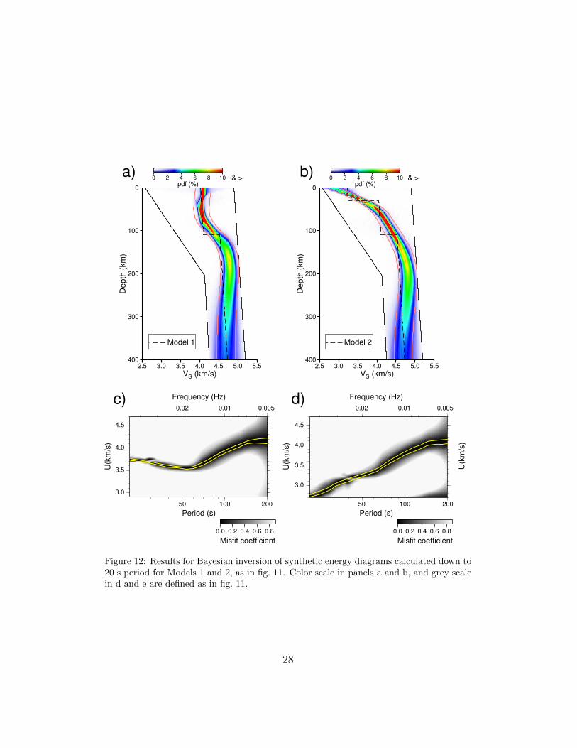
Figure 12: Results for Bayesian inversion of synthetic energy diagrams calculated down to20 s period for Models 1 and 2, as in fig. 11. Color scale in panels a and b, and grey scalein d and e are defined as in fig. 11.

28

periods, the depth of well resolved seismic structures within the Earth andMars extends to about 200 km, and 400 km, respectively, as expected fromMars’ radius, about half the Earth’s. Fig. 11a and b show that the distribu-tions of Bezier curves are in very good agreement with the expected profiles.An important result is that for the synthetic data (fig. 11a and b), the ±5%intervals around the median profiles of the distributions contain the inputmodels, which is one of the requirements of the InSight mission. For realdata (fig. 11c), VS values are globally lower than the PREM ones but thePREM is included in the ±5% interval.

The contours of the dispersion curves associated with the whole set ofaccepted models are plotted with yellow curves on the input dispersion dia-grams (fig. 11d–f). They all match with the area of low misfit coefficients,which means that a large range of possible models could produce such a dis-persion diagram. This good agreement between synthetic and tested dataclearly supports the method employed here for elucidating the seismic struc-ture of planetary mantles from a large number of models.

The terrestrial group velocity is not tightly constrained at periods shorterthan ∼60 seconds for the studied event (fig. 11f), and therefore does notresolve crustal velocities (fig. 11c). Given a similar frequency range, theMartian synthetic tests do differentiate between the two different end mem-ber crustal models (Models 1 and 2), but the crustal structure is still greatlysmoothed, particularly across the mid-crustal discontinuity in Model 2. Whilegetting reliable dispersion data to higher frequencies may be problematic withgreat-circle average approaches, it may be possible using smaller events lo-cated using other location approaches that become feasible as the averagemantle velocity is constrained by the large events located using the approachof this study. Synthetic tests with group velocity dispersion extended to 20seconds allow us to determine more details about Martian crustal structurewhen such data is available (fig. 12).

6. Discussion

This study is not intended to robustly constrain the location capabilitiesand uncertainties of the particular InSight instrument installation on the sur-face of Mars. That will, of course, depend on the still undetermined noisecharacteristics of Mars and the installation itself, as well as the unknownseismicity level of Mars. Based on modeling of Viking wind data, the micro-seismic noise on Mars with periods between 1 and 100 seconds is expected

29

to be less than that on Earth by roughly an order of magnitude (Lognonneand Mosser, 1993), and this is supported by more recent numerical calcula-tions based on large eddy simulations (Lognonne et al., 2012b). This study,however, is focused on demonstrating the effectiveness of an approach ofdetermining locations and inverting for interior structure based on multipleorbit surface wave recordings if the seismicity level of Mars and noise levelsof the InSight installation permit observations of such surface waves.

Further work is clearly necessary to work on enhancing techniques forobservations of multiple orbit surface waves with lower signal to noise ratios inorder to expand the range of this approach to lower event magnitudes and/orhigher installation noise levels. Undoubtedly, other techniques using bodywaves will be necessary to locate smaller nearby events, and it is important towork on making such locations more robust when the initial velocity model isnot well constrained, as will be the case in our initial observations on Mars.

7. Conclusions

Given the high quality design of the InSight experiment and current esti-mates of Martian seismicity, we have a high capability of detecting multipleorbit surface waves on Mars. Our study verifies that we can use such datarecorded on a single station for events just above the threshold for observ-ability of such signals. This data allows for location within ∼1◦ in epicentraldistance and 30 seconds in origin time, which is adequate to allow for recov-ery of mantle velocity structure within ±5% using inversion of P and S traveltimes for datasets with as few as 7 events. If we are able to record signals onthe horizontal components with sufficient signal to noise ratio, backazimuthdetermination allows for absolute locations within 10◦, which can localizethe seismic source within a tectonic region of the Martian surface. Finally,the multiple orbit surface waves allow for the determination of fundamentalmode group velocity dispersion independent of location error, which can moretightly resolve upper mantle velocities. Overall, such a single station datasetshould allow us to get relatively tight constraints on the interior structure ofMars, giving us unprecedented constraints on the structure and evolution ofanother terrestrial planet.

Acknowledgements

This work was undertaken during the preparation phase of the SEIS ex-periment on InSight mission. MP was supported by funds from NASA/JPL

30

as part of the InSight mission, and EB, MD, AM, and PL acknowledgethe financial support of CNES. The Bayesian inversions of group velocitydispersion diagrams were performed using HPC resources of CINES (Cen-tre Informatique National de lEnseignement Suprieur) under the allocation2014047062 made by GENCI (Grand Equipement National de Calcul Inten-sif).

References

Anderson, D., Miller, W., Latham, G., Nakamura, Y., Toksoz, M., 1977.Seismology on Mars. J. Geophys. Res. 82, 4524–4546.

Baker, G., Stevens, J., 2004. Backazimuth estimation reliability us-ing surface wave polarization. Geophys. Res. Lett. 31, L09611.doi:10.1029/2004GL019510.

Banerdt, W., Smrekar, S., Lognonne, P., Spohn, T., Asmar, S., Banfield,D., Boschi, L., Christensen, U., Dehant, V., Folkner, W., Giardini, D.,Goetze, W., Golombek, M., Grott, M., Hudson, T., Johnson, C., Kargl, G.,Kobayashi, N., Maki, J., Mimoun, D., Mocquet, A., Morgan, P., Panning,M., Pike, W., Tromp, J., van Zoest, T., Weber, R., Wieczorek, M., Garcia,R., Hurst, K., 2013. InSight: A Discovery mission to explore the interiorof Mars, in: 44th Lunar and Planetary Science Conference, Lunar andPlanetary Inst., Houston, TX. p. Abstract #1915.

Bezier, P., 1966. Definition numerique des courbes et surfaces I. Automatisme11, 625–632.

Bezier, P., 1967. Definition numerique des courbes et surfaces II. Automa-tisme 12, 17–21.

Bodin, T., Sambridge, M., Tkalcic, H., Arroucau, P., Gallagher, K., Rawlin-son, N., 2012. Transdimensional inversion of receiver functions and surfacewave dispersion. J. Geophys. Res. 117, B02301. doi:10.1029/2011JB008560.

Cammarano, F., Deuss, A., Goes, S., Giardini, D., 2005. One-dimensionalphysical reference models for the upper mantle and transition zone: com-bining seismic and mineral physics constraints. J. Geophys. Res. 110,B01306. doi:10.1029/2004JB003272.

31

Chael, E., 1997. An automated Rayleigh-wave detection algorithm. Bull.Seism. Soc. Amer. 87, 157–163.

Chenet, H., Lognonne, P., Wieczorek, M., Mizutani, H., 2006. Lateral vari-ations of lunar crustal thickness from the apollo seismic data set. EarthPlanet. Sci. Lett. 243, 1–14.

Crotwell, H., Owens, T., Ritsema, J., 1999. The TauP toolkit: Flexibleseismic travel-time and ray-path utilities. Seis. Res. Lett. 70, 154–160.

Dehant, V., Lognonne, P., Sotin, C., 2004. Netlander: a European missionto study the planet Mars. Planet. Space Sci. 52, 977–985.

Drilleau, M., Beucler, E., Mocquet, A., Verhoeven, O., Moebs, G., Burgos,G., Montagner, J.P., Vacher, P., 2013. A Bayesian approach to infer radialmodels of temperature and anisotropy in the transition zone from surfacewave dispersion curves. Geophys. J. Int. 195, 1165–1183.

Dziewonski, A., Anderson, D., 1981. Preliminary Reference Earth Model.Phys. Earth Planet. Inter. 25, 297–356.

Dziewonski, A., Woodhouse, J., 1983. An experiment in systematic study ofglobal seismicity: Centroid-moment tensor solutions for 201 moderate andlarge earthquakes of 1981. J. Geophys. Res. 88, 3247–3271.

Ekstrom, G., Nettles, M., Dziewonski, A., 2012. The global CMT project2004-2010: Centroid-moment tensors for 13,017 earthquakes. Phys. EarthPlanet. Inter. 200–201, 1–9.

Frohlich, C., Pulliam, J., 1999. Single-station location of seismic events:a review and a plea for more research. Phys. Earth Planet. Inter. 113,277–291.

Gagnepain-Beyneix, J., Lognonne, P., Chenet, H., Lombardi, D., Spohn, T.,2006. A seismic model of the lunar mantle and constraints on temperatureand mineralogy. Phys. Earth Planet. Inter. 159, 140–166.

Garcia, R., Gagnepain-Beyneix, J., Chevrot, S., Lognonne, P., 2011. Verypreliminary reference Moon model. Phys. Earth Planet. Inter. 188, 96–113.

32

Gilbert, F., Dziewonski, A., 1975. An application of normal mode theory tothe retrieval of structural parameters and source mechanisms from seismicspectra. Philos. Trans. R. Soc. London A 278, 187–269.

Golombek, M., 2002. A revision of Mars seismicity from surface faulting, in:33rd Lunar and Planetary Science Conference, Lunar and Planetary Inst.,Houston, TX. p. Abstract #1244.

Golombek, M., Banerdt, W., Tanaka, K., Tralli, D., 1992. A prediction ofMars seismicity from surface faulting. Science 258, 979–981.

Gudkova, T., Zharkov, V., 2004. Mars: interior sturcture and excitation offree oscillations. Phys. Earth Planet. Inter. 142, 1–22.

Hastings, W., 1970. Monte Carlo sampling methods using Markov chainsand their applications. Biometrika 57, 97–109.

Herglotz, G., 1907. Uber das benndorfsche Problem der Fortpflanzungs-geschwindigkeit der Erdbebenstrahlen. Zeitschrift fur Geophysik 8, 145–147.

Isaak, D., 1992. High-temperature elasticity of iron-bearing olivines. J.Geophys. Res. 97, 1871–1885.

Johnson, A., Kanter, L., 1990. Earthquakes in stable continental crust. Sci.Am. 262, 68–75.

Khan, A., Boschi, L., Connolly, A., 2009. On mantle chemical and thermalheterogeneities and anisotropy as mapped by inversion of global surfacewave data. J. Geophys. Res. 114, B09305. doi:10.1029/2009JB006399.

Khan, A., Connolly, J., 2008. Constraining the composition and thermalstate of Mars from inversion of geophysical data. J. Geophys. Res. 113,E07003. doi:10.1029/2007JE002996.

Khan, A., Connolly, J., Maclennan, J., Mosegaard, K., 2007. Joint inver-sion of seismic and gravity data for lunar composition and thermal state.Geophys. J. Int. 168, 243–258.

Khan, A., Mosegaard, K., 2002. An inquiry into the lunar interior: A non-linear inversion of the Apollo lunar seismic data. J. Geophys. Res. 107,5036. doi:10.1029/2001JE001658.

33

Khan, A., Zunino, A., Deschamps, F., 2013. Upper mantle compositionalvariations and discontinuity topography imaged beneath Australia frombayesian inversion of surface-wave phase velocities and thermochemicalmodeling. J. Geophys. Res. 116. doi:10.1002/jgrb.50304.

Knapmeyer, M., Oberst, J., Hauber, E., Wahlisch, M., Deuchler, C., Wag-ner, R., 2006. Working models for spatial distribution and level of Mars’seismicity. J. Geophys. Res. 111, E11006. doi:10.1029/2006JE002708.

Larmat, C., Montagner, J.P., Capdeville, Y., Banerdt, W., Lognonne, P.,Vilotte, J.P., 2008. Numerical assessment of the effects of topography andcrustal thickness on Martian seismograms using a coupled modal solution–spectral element method. Icarus 196, 78–89.

Lay, T., Wallace, T., 1995. Modern Global Seismology. Academic Press.

Linkin, V., Harri, A.M., Lipatov, A., Belostotskaja, K., Derbunovich, B.,Ekonomov, A., Khloustova, L., Kremnev, R., Makarov, V., Martinov, B.,Nenarokov, D., Prostov, M., Pustovalov, A., Shustko, G., Jarvinen, I.,Kivilinna, H., Korpela, S., Kumpulainen, K., Lehto, A., Pellinen, R., Pir-jola, R., Riihela, P., Salminen, A., Schmidt, W., Siili, T., Blamont, J., Car-pentier, T., Debus, A., Hua, C.T., Karczewski, J.F., Laplace, H., Levacher,P., Lognonne, P., Malique, C., Menvielle, M., Mouli, G., Pommereau, J.P.,Quotb, K., Runavot, J., Vienne, D., Grunthaner, F., Kuhnke, F., Mus-mann, G., Rieder, R., Wanke, H., Economou, T., Herring, M., Lane, A.,McKay, C.P., 1998. A sophisticated lander for scientific exploration ofMars: scientific objectives and implementation of the Mars-96 Small Sta-tion. Planet. Space Sci. 46, 717–737. doi:10.1016/S0032-0633(98)00008-7.

Lognonne, P., Banerdt, W.B., Hurst, K., Mimoun, D., Garcia, R., Lefeuvre,M., Gagnepain-Beyneix, J., Wieczorek, M., Mocquet, A., Panning, M.,Beucler, E., Deraucourt, S., Giardini, D., Boschi, L., Christensen, U.,Goetz, W., Pike, T., Johnson, C., Weber, R., Larmat, K., Kobayashi,N., Tromp, J., 2012a. Insight and Single-Station Broadband Seismology:From Signal and Noise to Interior Structure Determination, in: Lunar andPlanetary Institute Science Conference Abstracts, p. 1983.

Lognonne, P., Beyneix, J.G., Banerdt, W.B., Cacho, S., Karczewski, J.F.,Morand, M., 1996. Ultra broad band seismology on InterMarsNet. Planet.Space Sci. 44, 1237. doi:10.1016/S0032-0633(96)00083-9.

34

Lognonne, P., Clevede, E., Kanamori, H., 1998. Computation of seismogramsand atmospheric oscillations by normal-mode summation for a sphericalearth model with realistic atmosphere. Geophys. J. Int. 135, 388–406.

Lognonne, P., Gagnepain-Beyneix, J., Banerdt, W., Chenet, H., 2003. A newseismic model of the Moon: implication in terms of structure, formation,and evolution. Earth Planet. Sci. Lett. 211, 27–44.

Lognonne, P., Giardini, D., Banerdt, W., Gagnepain-Beyneix, J., Mocquet,A., Spohn, T., Karczewski, J., Schibler, P., Cacho, S., Pike, W., Cavoit, C.,Desautez, A., Favede, M., Gabsi, T., Simoulin, L., Striebig, N., Campillo,M., Deschamp, A., Hinderer, J., Leveque, J., Montagner, J.P., Rivera, L.,Benz, W., Breuer, D., Defraigne, P., Dehant, V., Fujimura, A., Mizutani,H., Oberst, J., 2000. The NetLander very broad band seismometer. Planet.Space Sci. 48, 1289–1302.

Lognonne, P., Johnson, C., 2007. Planetary seismology, in: Schubert, G.(Ed.), Treatise on Geophysics. Elsevier, Amsterdam. volume 10, pp. 69–122.

Lognonne, P., Mosser, B., 1993. Planetary seismology. Surveys Geophys. 14,239–302.

Lognonne, P., Spiga, A., Hurst, K., Gabsi, T., Banfield, D., de Raucort, S.,Mimoun, D., Banerdt, W., Hecht, M., 2012b. Atmospheric induced micro-seismic noise generation: Large eddy simulations, in: Lunar and PlanetaryInstitute Science Conference Abstracts, p. 1994.

McSween, H., 1994. What we have learned about Mars from SNC meteorites.Meteoritics 29, 757–779.

Metropolis, N., Rosenbluth, A., Rosenbluth, M., Teller, A., Teller, E., 1953.Equation of state calculations by fast computing machines. J. Chem. Phys.21, 1087–1091.

Mimoun, D., Lognonne, P., Banerdt, W.B., Hurst, K., Deraucourt, S.,Gagnepain-Beyneix, J., Pike, T., Calcutt, S., Bierwirth, M., Roll, R.,Zweifel, P., Mance, D., Robert, O., Nebut, T., Tillier, S., Laudet, P.,Kerjean, L., Perez, R., Giardini, D., Christenssen, U., Garcia, R., 2012.The InSight SEIS Experiment, in: Lunar and Planetary Institute ScienceConference Abstracts, p. 1493.

35

Mocquet, A., Rosenblatt, P., Dehant, V., Verhoeven, O., 2011. The deepinterior of Venus, Mars, and the Earth: A brief review and the need forplanetary surface-based measurements. Planet. Space Sci. 59, 1048–1061.doi:10.1016/j.pss.2010.02.002.

Mocquet, A., Vacher, P., Grasset, O., Sotin, C., 1996. Theoretical seismicmodels of Mars: the importance of the iron content of the mantle. Planet.Space Sci. 44, 1251–1268.

Mosca, I., Cobden, L., Deuss, A., Ritsema, J., Trampert, J., 2012. Seis-mic and mineralogical structures of the lower mantle from probabilistictomography. J. Geophys. Res. 117, B06304. doi:10.1029/2011JB008851.

Mosegaard, K., Tarantola, A., 1995. Monte-Carlo sampling of solutions toinverse problems. J. Geophys. Res. 100, 12431–12447.

Nakamura, Y., 1983. Seismic velocity structure of the lunar mantle. J.Geophys. Res. 88, 677–686.

Nakamura, Y., Latham, G., Dorman, H., Ibrahim, A.B., Koyama, J., Hor-varth, P., 1979. Shallow moonquakes - depth, distribution and implicationsas to the present state of the lunar interior, in: Proc. Lunar Planet. Sci.Conf. 10th, pp. 2299–2309.

Neumann, G., Zuber, M., Wieczorek, M., McGovern, P., Lemoine, F., Smith,D., 2004. Crustal structure of Mars from gravity and topography. J.Geophys. Res. 109, E08002. doi:10.1029/2004JE002262.

Nimmo, F., 2002. Admittance estimates of mean crustal thickness and den-sity at the Martian hemispheric dichotomy. J. Geophys. Res. 107, 5117.doi:10.1029/2000JE001488.

Nimmo, F., Faul, U.H., 2013. Dissipation at tidal and seismic frequen-cies in a melt-free, anhydrousaamars. J. Geophys. Res. 118, 2558–2569.doi:10.1002/2013JE004499.

Nimmo, F., Stevenson, D., 2001. Estimates of Martian crustal thickness fromviscous relaxation of topography. J. Geophys. Res. 106, 5085–5098.

Okal, E., Sweet, J., 2007. Frequency-size distributions for intraplate earth-quakes. GSA Special Papers 425, 59–71.

36

Phillips, R., 1991. Expected rate of marsquakes, in: Scientifc Rationale andRequirements for a Global Seismic Network on Mars. LPI Tech. Rept.,91-02, Lunar and Planetary Inst., Houston, pp. 35–38.

Phinney, R., 1964. Structure of the Earth’s crust from spectral behavior oflong-period body waves. J. Geophys. Res. 69, 2997–3017.

Rivoldini, A., Van Hoolst, T., Verhoeven, O., Mocquet, A., Dehant, V.,2011. Geodesy constraints on the interior structure and composition ofMars. Icarus 213, 451–472.

Shapiro, N., Ritzwoller, M., 2002. Monte-Carlo inversion for a global shear-velocity model of the crust and upper mantle. Geophys. J. Int. 151, 88–105.

Shen, W., Ritzwoller, M., Schulte-Pelkum, V., 2013a. A 3-D model of thecrust and uppermost mantle beneath the central and western US by jointinversion of receiver functions and surface wave dispersion. J. Geophys.Res. 118, 262–276.

Shen, W., Ritzwoller, M., Schulte-Pelkum, V., Lin, F., 2013b. Joint inversionof surface wave dispersion and receiver functions: a Bayesian Monte-Carloapproach. Geophys. J. Int. 192, 807–836.

Sohl, F., Schubert, G., 2007. Interior structure, composition, and mineralogyof the terrestrial planets, in: Spohn, T., Schubert, G. (Eds.), Treatise onGeophysics. Elsevier. volume 10, pp. 27–68.

Sohl, F., Schubert, G., Spohn, T., 2005. Geophysical constraints on thecomposition and structure of the Martian interior. J. Geophys. Res. 110,E12008. doi:10.1029/2005JE002520.

Sohl, F., Spohn, T., 1997. The interior structure of Mars: Implications fromSNC meteorites. J. Geophys. Res. 102, 1613–1635.

Solomon, S., Anderson, D., Banerdt, W., Butler, R., Davis, P., Duennebier,F., Nakamura, Y., Okal, E., Phillips, R., 1991. Scientific rationale andrequirements for a global seismic network on Mars, LPI Tech. Rept. 91-02.Lunar and Planetary Inst., Houston, TX.

Tanimoto, T., Rivera, L., 2005. Prograde Rayleigh wave particle motion.Geophys. J. Int. 162, 399–405. doi:10.1111/j.1365-246X.2005.02481.x.

37

Verhoeven, O., Rivoldini, A., Vacher, P., Mocquet, A., Choblet, G., Men-vielle, M., Dehant, V., Van Hoolst, T., Sleewaegen, J., Barriot, J.P.,Lognonne, P., 2005. Interior structure of terrestrial planets: ModelingMars’ mantle and its electromagnetic, geodetic, and seismic properties. J.Geophys. Res. 110, E04009. doi:10.1029/2004JE002271.

Vinnik, L., Chenet, H., Gagnepain-Beyneix, J., Lognonne, P., 2001. Firstseismic receiver functions on the Moon. Geophys. Res. Lett. 28, 3031–3034.

Weber, R., Lin, P.Y., Garnero, E., Williams, Q., Lognonne, P., 2011. Seismicdetection of the lunar core. Science 331, 309–312.

Wiechert, E., 1910. Bestimmung des weges der Erdbebenwellen imErdinnern. I. Theroetisches. Phys. Z. 11, 294–304.

Wieczorek, M., Zuber, M., 2004. Thickness of the Martian crust: Improvedconstraints from geoid-to-topography ratios. J. Geophys. Res. 109, E01009.doi:10.1029/2003JE002153.

Woodhouse, J., 1988. The calculation of eigenfrequencies and eigenfunctionsof the free oscillations of the earth and the sun, in: Doornbos, D. (Ed.),Seismological Algorithms. Academic Press, London, pp. 321–370.

Zuber, M., Solomon, S., Phillips, R., Smith, D., Tyler, G., Aharonson, O.,Balmino, G., Banerdt, W., Head, J., Johnson, C., Lemoine, F., McGovern,P., Neumann, G., Rowlands, D., Zhong, S., 2000. Internal structure andearly thermal evolution of Mars from Mars Global Surveyor topographyand gravity. Science 287, 1788–1793.

38