UPTEC IT 10 016

Examensarbete 30 hpJuni 2010

Verifying Finite State Machine Behavior Using QuickCheck Eqc_fsm

Ida LindgrenRobin Malmros

Teknisk- naturvetenskaplig fakultet UTH-enheten Besöksadress: Ångströmlaboratoriet Lägerhyddsvägen 1 Hus 4, Plan 0 Postadress: Box 536 751 21 Uppsala Telefon: 018 – 471 30 03 Telefax: 018 – 471 30 00 Hemsida: http://www.teknat.uu.se/student

Abstract

Verifying Finite State Machine Behavior UsingQuickCheck Eqc_fsm

Ida Lindgren and Robin Malmros

In order to communicate properly, mobile telephones connect to base transceiverstations which forward the telephones’ signals. These base transceiver stations arecalled Node Bs.As the use of mobile telephones expands every day, the number of Node Bs in theworld increases with rapid speed. This requires better software systems in the NodeBs, so people can use their mobile telephones whenever and wherever, without anyobstacles in the way.Better testing tools are needed to ensure the quality of the software systems in theNode Bs. This thesis is based on the evaluation of a software testing tool calledQuickCheck and especially one of its modules, eqc_fsm.The goal was to determine if the characteristics of two subsystems in Node B wouldmake QuickCheck and its module applicable as a testing tool for those systems. SinceQuickCheck can be used to test systems modeled as finite state machines, the twosubsystems were modeled as numerous uniquely finite state machines and testedusing QuickCheck.The systems were both successfully modeled according to eqc_fsm and tested usingQuickCheck. The applicability of eqc_fsm as a testing tool was not affected to a greatdegree by the systems characteristics that were investigated. Eqc_fsm was alsoflexible to handle systems with different characteristics. This showed thatQuickCheck’s eqc_fsm module was applicable as a testing tool for the twosubsystems in Node B. QuickCheck and its module eqc_fsm can be used to improvethe quality of the software systems in Node B.

Tryckt av: Reprocentralen ITCISSN: 1401-5749, UPTEC IT 10 016Examinator: Anders JanssonÄmnesgranskare: Lars-Henrik ErikssonHandledare: Daniel Jernberg

Sammanfattning

I ett radionät ansluter mobiltelfoner och andra enheter till radiobasstationer, vilka förmedl-ar signaler mellan enheter. En sådan radiobasstation kallas också för en Node B. Idag används mobiltelefoner i allt större utsträckning än tidigare, vilket innebär att antalet Node Bs i världen ökar markant. Samtidigt ökar komplexiteten på mjukvaran i Node B. Det här ställer krav på att testmetoder och testverktyg blir mer effektiva för att säkerställa kvaliteten på mjukvaran. Detta var anledningen till att det här examensarbete utfördes eftersom Node Bs är en viktig produkt hos företaget där detta examensarbete utfördes. Företaget kommer av sekretesskäl fortsättningsvis i denna rapport refereras till som the Leading Telecom Company (LTC). Problemdefinitionen för detta examensarbete var att fastställa om karaktäristikerna hos en mjukvara gör QuickChecks Erlang QuickCheck Finite State Machine (eqc_fsm) modul applicerbar som ett testverktyg för denna mjukvara. Även att undersöka om eqc_fsm är ett lämpligt verktyg för att testa LTC’s Node B Main Processing Software (MPSW).Två avgränsade delar av LTC’s MPSW modellerades som finita tillståndsmaskiner och tes-tades med QuickCheck. Det fanns flera anledningar till att dessa två delsystem valdes. De förväntades sakna komplexa interaktioner med andra delar av systemet och vara tillräckligt små för att kompletta tester av delsystemen skulle kunna designas och utföras inom tidsra-men för detta examensarbete. Ett antal karaktäristiker hos dessa två delsystem identifi-erades och utvärderades baserat på hur de påverkade applicerbarheten av QuickChecks eqc_fsm modul som ett testverktyg för systemen.Karaktäristikerna som utvärderades var att de två delsystemen hade:

• Få interaktioner och beroenden med andra system

• Få naturliga tillstånd i delsystemen

• Få parametrar i signalerna som används för att kommunicera med delsystemen

• Få övergångar i tillståndsmaskinerna av delsystemen

Applicerbarheten av eqc_fsm som ett testverktyg för en mjukvara påverkades inte nämnv-ärt av de karaktäristikerna som undersöktes. Eqc_fsm fungerade bra tillsammans med system som hade dessa karaktäristiker. Eqc_fsm var flexibelt och kunde hantera system med olika karaktäristiker.Eqc_fsm visade sig vara applicerbart som ett testverktyg för de två avgränsade delsyste-men, vilket indikerar att QuickChecks eqc_fsm modul skulle kunna vara ett lämpligt tes-tverktyg för LTCs Node B mjukvara.

I

Abbreviations

2G Second Generation3G Third Generation3GPP 3rd Generation Partnership ProjectCDMA Code Division Multiple AccessCN Core NetworkCT Common TestEC Equipment ControlEP Elementary ProcedureEqc_fsm Erlang QuickCheck Finite State MachineEqc_statem Erlang QuickCheck State MachineFACH Forward Access ChannelGSM Global System for Mobile CommunicationsIE Information ElementITU International Telecommunication UnionLTC Leading Telecom CompanyMPSW Main Processing SoftwareNBAP Node B Application PartNPR Non Processing ResourcesPCH Paging ChannelRACH Random Access ChannelRNC Radio Network ControllerSUT System Under TestUE User EquipmentWCDMA Wideband Code Division Multiple Access

II

Table of Contents

CHAPTER 1 Introduction . . . . . . . . . . . . . . . . . . . . . . . . . . . . . . . . . . . . . . . . . . . . . .1

1.1 Background . . . . . . . . . . . . . . . . . . . . . . . . . . . . . . . . . . . . . . . . . . . . . . . . . . . . . . . . . . . . . . . . . . . 11.2 Problem Definition . . . . . . . . . . . . . . . . . . . . . . . . . . . . . . . . . . . . . . . . . . . . . . . . . . . . . . . . . . . . . 11.3 Scope . . . . . . . . . . . . . . . . . . . . . . . . . . . . . . . . . . . . . . . . . . . . . . . . . . . . . . . . . . . . . . . . . . . . . . . . 11.4 Goal . . . . . . . . . . . . . . . . . . . . . . . . . . . . . . . . . . . . . . . . . . . . . . . . . . . . . . . . . . . . . . . . . . . . . . . . . 2

CHAPTER 2 Technical Background . . . . . . . . . . . . . . . . . . . . . . . . . . . . . . . . . . . . . .3

2.1 Radio Network. . . . . . . . . . . . . . . . . . . . . . . . . . . . . . . . . . . . . . . . . . . . . . . . . . . . . . . . . . . . . . . . . 32.1.1 3rd Generation Partnership Project . . . . . . . . . . . . . . . . . . . . . . . . . . . . . . . . . . . . . . . . . . . . . . 32.1.2 Wideband Code Division Multiple Access . . . . . . . . . . . . . . . . . . . . . . . . . . . . . . . . . . . . . . . . 32.1.3 Node B . . . . . . . . . . . . . . . . . . . . . . . . . . . . . . . . . . . . . . . . . . . . . . . . . . . . . . . . . . . . . . . . . . . . 42.1.4 RNC . . . . . . . . . . . . . . . . . . . . . . . . . . . . . . . . . . . . . . . . . . . . . . . . . . . . . . . . . . . . . . . . . . . . . . 52.1.5 Transport Channels . . . . . . . . . . . . . . . . . . . . . . . . . . . . . . . . . . . . . . . . . . . . . . . . . . . . . . . . . . 5

2.2 Node B Application Part . . . . . . . . . . . . . . . . . . . . . . . . . . . . . . . . . . . . . . . . . . . . . . . . . . . . . . . . . 62.2.1 Elementary Procedures . . . . . . . . . . . . . . . . . . . . . . . . . . . . . . . . . . . . . . . . . . . . . . . . . . . . . . . 62.2.2 Information Elements. . . . . . . . . . . . . . . . . . . . . . . . . . . . . . . . . . . . . . . . . . . . . . . . . . . . . . . . . 7

2.3 Erlang. . . . . . . . . . . . . . . . . . . . . . . . . . . . . . . . . . . . . . . . . . . . . . . . . . . . . . . . . . . . . . . . . . . . . . . . 72.3.1 History . . . . . . . . . . . . . . . . . . . . . . . . . . . . . . . . . . . . . . . . . . . . . . . . . . . . . . . . . . . . . . . . . . . . 72.3.2 General. . . . . . . . . . . . . . . . . . . . . . . . . . . . . . . . . . . . . . . . . . . . . . . . . . . . . . . . . . . . . . . . . . . . 72.3.3 Records . . . . . . . . . . . . . . . . . . . . . . . . . . . . . . . . . . . . . . . . . . . . . . . . . . . . . . . . . . . . . . . . . . . 8

2.4 Interfaces . . . . . . . . . . . . . . . . . . . . . . . . . . . . . . . . . . . . . . . . . . . . . . . . . . . . . . . . . . . . . . . . . . . . . 82.4.1 General Node B Interfaces. . . . . . . . . . . . . . . . . . . . . . . . . . . . . . . . . . . . . . . . . . . . . . . . . . . . . 82.4.2 Test Environment. . . . . . . . . . . . . . . . . . . . . . . . . . . . . . . . . . . . . . . . . . . . . . . . . . . . . . . . . . . . 9

2.5 QuickCheck . . . . . . . . . . . . . . . . . . . . . . . . . . . . . . . . . . . . . . . . . . . . . . . . . . . . . . . . . . . . . . . . . . 102.5.1 Background . . . . . . . . . . . . . . . . . . . . . . . . . . . . . . . . . . . . . . . . . . . . . . . . . . . . . . . . . . . . . . . 102.5.2 Symbolic Representation . . . . . . . . . . . . . . . . . . . . . . . . . . . . . . . . . . . . . . . . . . . . . . . . . . . . . 102.5.3 Specification . . . . . . . . . . . . . . . . . . . . . . . . . . . . . . . . . . . . . . . . . . . . . . . . . . . . . . . . . . . . . . 11

2.5.3.1 Properties . . . . . . . . . . . . . . . . . . . . . . . . . . . . . . . . . . . . . . . . . . . . . . . . . . . . . . . . . . . . . . 112.5.3.2 Generators . . . . . . . . . . . . . . . . . . . . . . . . . . . . . . . . . . . . . . . . . . . . . . . . . . . . . . . . . . . . . 13

2.5.4 Shrinking . . . . . . . . . . . . . . . . . . . . . . . . . . . . . . . . . . . . . . . . . . . . . . . . . . . . . . . . . . . . . . . . . 142.5.5 Finite State Machines. . . . . . . . . . . . . . . . . . . . . . . . . . . . . . . . . . . . . . . . . . . . . . . . . . . . . . . . 15

2.5.5.1 Erlang QuickCheck State Machine . . . . . . . . . . . . . . . . . . . . . . . . . . . . . . . . . . . . . . . . . . 152.5.5.2 Initial_state. . . . . . . . . . . . . . . . . . . . . . . . . . . . . . . . . . . . . . . . . . . . . . . . . . . . . . . . . . . . . 162.5.5.3 Command . . . . . . . . . . . . . . . . . . . . . . . . . . . . . . . . . . . . . . . . . . . . . . . . . . . . . . . . . . . . . . 172.5.5.4 Precondition . . . . . . . . . . . . . . . . . . . . . . . . . . . . . . . . . . . . . . . . . . . . . . . . . . . . . . . . . . . . 172.5.5.5 Next_state. . . . . . . . . . . . . . . . . . . . . . . . . . . . . . . . . . . . . . . . . . . . . . . . . . . . . . . . . . . . . . 172.5.5.6 Postcondition . . . . . . . . . . . . . . . . . . . . . . . . . . . . . . . . . . . . . . . . . . . . . . . . . . . . . . . . . . . 18

2.5.6 Erlang QuickCheck Finite State Machine . . . . . . . . . . . . . . . . . . . . . . . . . . . . . . . . . . . . . . . . 182.5.6.1 Goals with Eqc_fsm. . . . . . . . . . . . . . . . . . . . . . . . . . . . . . . . . . . . . . . . . . . . . . . . . . . . . . 192.5.6.2 The Changes. . . . . . . . . . . . . . . . . . . . . . . . . . . . . . . . . . . . . . . . . . . . . . . . . . . . . . . . . . . . 192.5.6.3 New Features . . . . . . . . . . . . . . . . . . . . . . . . . . . . . . . . . . . . . . . . . . . . . . . . . . . . . . . . . . . 21

III

CHAPTER 3 Previous Work . . . . . . . . . . . . . . . . . . . . . . . . . . . . . . . . . . . . . . . . . . .23

3.1 NBAP Message Construction Using QuickCheck. . . . . . . . . . . . . . . . . . . . . . . . . . . . . . . . . . . . . 233.1.1 Purpose. . . . . . . . . . . . . . . . . . . . . . . . . . . . . . . . . . . . . . . . . . . . . . . . . . . . . . . . . . . . . . . . . . . 233.1.2 Task . . . . . . . . . . . . . . . . . . . . . . . . . . . . . . . . . . . . . . . . . . . . . . . . . . . . . . . . . . . . . . . . . . . . . 233.1.3 Implementation . . . . . . . . . . . . . . . . . . . . . . . . . . . . . . . . . . . . . . . . . . . . . . . . . . . . . . . . . . . . 243.1.4 Conclusion . . . . . . . . . . . . . . . . . . . . . . . . . . . . . . . . . . . . . . . . . . . . . . . . . . . . . . . . . . . . . . . . 24

3.2 Testing a Radiotherapy Support System With QuickCheck . . . . . . . . . . . . . . . . . . . . . . . . . . . . . 243.2.1 Purpose. . . . . . . . . . . . . . . . . . . . . . . . . . . . . . . . . . . . . . . . . . . . . . . . . . . . . . . . . . . . . . . . . . . 243.2.2 Task . . . . . . . . . . . . . . . . . . . . . . . . . . . . . . . . . . . . . . . . . . . . . . . . . . . . . . . . . . . . . . . . . . . . . 243.2.3 Implementation . . . . . . . . . . . . . . . . . . . . . . . . . . . . . . . . . . . . . . . . . . . . . . . . . . . . . . . . . . . . 253.2.4 Conclusion . . . . . . . . . . . . . . . . . . . . . . . . . . . . . . . . . . . . . . . . . . . . . . . . . . . . . . . . . . . . . . . . 25

3.3 A Comparison With Two Master Theses Using QuickCheck. . . . . . . . . . . . . . . . . . . . . . . . . . . . 25

CHAPTER 4 Methodology . . . . . . . . . . . . . . . . . . . . . . . . . . . . . . . . . . . . . . . . . . . . .27

4.1 Literature studies . . . . . . . . . . . . . . . . . . . . . . . . . . . . . . . . . . . . . . . . . . . . . . . . . . . . . . . . . . . . . . 274.1.1 QuickCheck Course for Erlang Users . . . . . . . . . . . . . . . . . . . . . . . . . . . . . . . . . . . . . . . . . . . 274.1.2 QuickCheck Literature. . . . . . . . . . . . . . . . . . . . . . . . . . . . . . . . . . . . . . . . . . . . . . . . . . . . . . . 274.1.3 Erlang Basic Course. . . . . . . . . . . . . . . . . . . . . . . . . . . . . . . . . . . . . . . . . . . . . . . . . . . . . . . . . 274.1.4 Network Architecture. . . . . . . . . . . . . . . . . . . . . . . . . . . . . . . . . . . . . . . . . . . . . . . . . . . . . . . . 274.1.5 NBAP. . . . . . . . . . . . . . . . . . . . . . . . . . . . . . . . . . . . . . . . . . . . . . . . . . . . . . . . . . . . . . . . . . . . 284.1.6 Interfaces and Applications . . . . . . . . . . . . . . . . . . . . . . . . . . . . . . . . . . . . . . . . . . . . . . . . . . . 28

4.2 Practical Work . . . . . . . . . . . . . . . . . . . . . . . . . . . . . . . . . . . . . . . . . . . . . . . . . . . . . . . . . . . . . . . . 284.2.1 Testing at LTC, General Studies . . . . . . . . . . . . . . . . . . . . . . . . . . . . . . . . . . . . . . . . . . . . . . . 284.2.2 Manual Testing at LTC . . . . . . . . . . . . . . . . . . . . . . . . . . . . . . . . . . . . . . . . . . . . . . . . . . . . . . 284.2.3 SUT . . . . . . . . . . . . . . . . . . . . . . . . . . . . . . . . . . . . . . . . . . . . . . . . . . . . . . . . . . . . . . . . . . . . . 284.2.4 Running QuickCheck. . . . . . . . . . . . . . . . . . . . . . . . . . . . . . . . . . . . . . . . . . . . . . . . . . . . . . . . 28

CHAPTER 5 Technical Solution . . . . . . . . . . . . . . . . . . . . . . . . . . . . . . . . . . . . . . . .29

5.1 Equipment Control. . . . . . . . . . . . . . . . . . . . . . . . . . . . . . . . . . . . . . . . . . . . . . . . . . . . . . . . . . . . . 295.1.1 SUT Description . . . . . . . . . . . . . . . . . . . . . . . . . . . . . . . . . . . . . . . . . . . . . . . . . . . . . . . . . . . 295.1.2 SUT Finite State Machine Model . . . . . . . . . . . . . . . . . . . . . . . . . . . . . . . . . . . . . . . . . . . . . . 30

5.1.2.1 Model 1 . . . . . . . . . . . . . . . . . . . . . . . . . . . . . . . . . . . . . . . . . . . . . . . . . . . . . . . . . . . . . . . 305.1.2.2 Model 2 . . . . . . . . . . . . . . . . . . . . . . . . . . . . . . . . . . . . . . . . . . . . . . . . . . . . . . . . . . . . . . . 31

5.1.3 QuickCheck Implementation . . . . . . . . . . . . . . . . . . . . . . . . . . . . . . . . . . . . . . . . . . . . . . . . . . 325.1.3.1 Model 1 . . . . . . . . . . . . . . . . . . . . . . . . . . . . . . . . . . . . . . . . . . . . . . . . . . . . . . . . . . . . . . . 325.1.3.2 Model 2 . . . . . . . . . . . . . . . . . . . . . . . . . . . . . . . . . . . . . . . . . . . . . . . . . . . . . . . . . . . . . . . 33

5.1.4 Results . . . . . . . . . . . . . . . . . . . . . . . . . . . . . . . . . . . . . . . . . . . . . . . . . . . . . . . . . . . . . . . . . . . 365.2 Transport Channels . . . . . . . . . . . . . . . . . . . . . . . . . . . . . . . . . . . . . . . . . . . . . . . . . . . . . . . . . . . . 37

5.2.1 SUT Description . . . . . . . . . . . . . . . . . . . . . . . . . . . . . . . . . . . . . . . . . . . . . . . . . . . . . . . . . . . 375.2.2 SUT Finite State Machine Model . . . . . . . . . . . . . . . . . . . . . . . . . . . . . . . . . . . . . . . . . . . . . . 37

5.2.2.1 Model 1 . . . . . . . . . . . . . . . . . . . . . . . . . . . . . . . . . . . . . . . . . . . . . . . . . . . . . . . . . . . . . . . 375.2.2.2 Model 2 . . . . . . . . . . . . . . . . . . . . . . . . . . . . . . . . . . . . . . . . . . . . . . . . . . . . . . . . . . . . . . . 395.2.2.3 Model 3 . . . . . . . . . . . . . . . . . . . . . . . . . . . . . . . . . . . . . . . . . . . . . . . . . . . . . . . . . . . . . . . 39

5.2.3 QuickCheck implementation . . . . . . . . . . . . . . . . . . . . . . . . . . . . . . . . . . . . . . . . . . . . . . . . . . 405.2.3.1 Model 1 . . . . . . . . . . . . . . . . . . . . . . . . . . . . . . . . . . . . . . . . . . . . . . . . . . . . . . . . . . . . . . . 40

IV

5.2.3.2 Model 2 . . . . . . . . . . . . . . . . . . . . . . . . . . . . . . . . . . . . . . . . . . . . . . . . . . . . . . . . . . . . . . . 415.2.3.3 Model 3 . . . . . . . . . . . . . . . . . . . . . . . . . . . . . . . . . . . . . . . . . . . . . . . . . . . . . . . . . . . . . . . 42

5.2.4 Results . . . . . . . . . . . . . . . . . . . . . . . . . . . . . . . . . . . . . . . . . . . . . . . . . . . . . . . . . . . . . . . . . . . 435.3 Fictive System . . . . . . . . . . . . . . . . . . . . . . . . . . . . . . . . . . . . . . . . . . . . . . . . . . . . . . . . . . . . . . . . 44

5.3.1 SUT Description . . . . . . . . . . . . . . . . . . . . . . . . . . . . . . . . . . . . . . . . . . . . . . . . . . . . . . . . . . . 445.3.2 SUT Finite State Machine Model . . . . . . . . . . . . . . . . . . . . . . . . . . . . . . . . . . . . . . . . . . . . . . 45

CHAPTER 6 Analysis . . . . . . . . . . . . . . . . . . . . . . . . . . . . . . . . . . . . . . . . . . . . . . . . .47

6.1 EC Characteristics Analysis. . . . . . . . . . . . . . . . . . . . . . . . . . . . . . . . . . . . . . . . . . . . . . . . . . . . . . 476.1.1 Few Interactions and Dependencies. . . . . . . . . . . . . . . . . . . . . . . . . . . . . . . . . . . . . . . . . . . . . 476.1.2 Few Natural States . . . . . . . . . . . . . . . . . . . . . . . . . . . . . . . . . . . . . . . . . . . . . . . . . . . . . . . . . . 476.1.3 Few Parameters . . . . . . . . . . . . . . . . . . . . . . . . . . . . . . . . . . . . . . . . . . . . . . . . . . . . . . . . . . . . 486.1.4 Few Transitions Between the States . . . . . . . . . . . . . . . . . . . . . . . . . . . . . . . . . . . . . . . . . . . . 48

6.2 Transport Channels Characteristics Analysis . . . . . . . . . . . . . . . . . . . . . . . . . . . . . . . . . . . . . . . . 486.2.1 Few Interactions and Dependencies. . . . . . . . . . . . . . . . . . . . . . . . . . . . . . . . . . . . . . . . . . . . . 486.2.2 Few Natural States . . . . . . . . . . . . . . . . . . . . . . . . . . . . . . . . . . . . . . . . . . . . . . . . . . . . . . . . . . 496.2.3 Few Parameters . . . . . . . . . . . . . . . . . . . . . . . . . . . . . . . . . . . . . . . . . . . . . . . . . . . . . . . . . . . . 496.2.4 Few Transitions Between the States . . . . . . . . . . . . . . . . . . . . . . . . . . . . . . . . . . . . . . . . . . . . 49

6.3 Test Results Analysis. . . . . . . . . . . . . . . . . . . . . . . . . . . . . . . . . . . . . . . . . . . . . . . . . . . . . . . . . . . 506.4 Fictive SUT Characteristics Analysis . . . . . . . . . . . . . . . . . . . . . . . . . . . . . . . . . . . . . . . . . . . . . . 50

6.4.1 Documentation. . . . . . . . . . . . . . . . . . . . . . . . . . . . . . . . . . . . . . . . . . . . . . . . . . . . . . . . . . . . . 506.4.2 Interactions and Dependencies . . . . . . . . . . . . . . . . . . . . . . . . . . . . . . . . . . . . . . . . . . . . . . . . 506.4.3 States and Transitions . . . . . . . . . . . . . . . . . . . . . . . . . . . . . . . . . . . . . . . . . . . . . . . . . . . . . . . 506.4.4 Parameters . . . . . . . . . . . . . . . . . . . . . . . . . . . . . . . . . . . . . . . . . . . . . . . . . . . . . . . . . . . . . . . . 51

CHAPTER 7 Discussion . . . . . . . . . . . . . . . . . . . . . . . . . . . . . . . . . . . . . . . . . . . . . . .53

7.1 The SUTs . . . . . . . . . . . . . . . . . . . . . . . . . . . . . . . . . . . . . . . . . . . . . . . . . . . . . . . . . . . . . . . . . . . . 537.2 The Work . . . . . . . . . . . . . . . . . . . . . . . . . . . . . . . . . . . . . . . . . . . . . . . . . . . . . . . . . . . . . . . . . . . . 53

7.2.1 Obtaining Knowledge . . . . . . . . . . . . . . . . . . . . . . . . . . . . . . . . . . . . . . . . . . . . . . . . . . . . . . . 537.2.2 Critical Revise of the Methods Used . . . . . . . . . . . . . . . . . . . . . . . . . . . . . . . . . . . . . . . . . . . . 54

7.3 The Result . . . . . . . . . . . . . . . . . . . . . . . . . . . . . . . . . . . . . . . . . . . . . . . . . . . . . . . . . . . . . . . . . . . 547.4 What Could Have Been Done Better. . . . . . . . . . . . . . . . . . . . . . . . . . . . . . . . . . . . . . . . . . . . . . . 547.5 Experiences . . . . . . . . . . . . . . . . . . . . . . . . . . . . . . . . . . . . . . . . . . . . . . . . . . . . . . . . . . . . . . . . . . 55

CHAPTER 8 Conclusion . . . . . . . . . . . . . . . . . . . . . . . . . . . . . . . . . . . . . . . . . . . . . . .57

CHAPTER 9 Future work . . . . . . . . . . . . . . . . . . . . . . . . . . . . . . . . . . . . . . . . . . . . .59

CHAPTER 10 References . . . . . . . . . . . . . . . . . . . . . . . . . . . . . . . . . . . . . . . . . . . . . .61

10.1 Literature . . . . . . . . . . . . . . . . . . . . . . . . . . . . . . . . . . . . . . . . . . . . . . . . . . . . . . . . . . . . . . . . . . . 6110.1.1 Books . . . . . . . . . . . . . . . . . . . . . . . . . . . . . . . . . . . . . . . . . . . . . . . . . . . . . . . . . . . . . . . . . . . 6110.1.2 Articles. . . . . . . . . . . . . . . . . . . . . . . . . . . . . . . . . . . . . . . . . . . . . . . . . . . . . . . . . . . . . . . . . . 6110.1.3 Technical Specifications . . . . . . . . . . . . . . . . . . . . . . . . . . . . . . . . . . . . . . . . . . . . . . . . . . . . 6110.1.4 Internet Sources . . . . . . . . . . . . . . . . . . . . . . . . . . . . . . . . . . . . . . . . . . . . . . . . . . . . . . . . . . . 6210.1.5 LTC’s Classified Documents. . . . . . . . . . . . . . . . . . . . . . . . . . . . . . . . . . . . . . . . . . . . . . . . . 6210.1.6 Software files . . . . . . . . . . . . . . . . . . . . . . . . . . . . . . . . . . . . . . . . . . . . . . . . . . . . . . . . . . . . . 62

V

CHAPTER 11 Appendix . . . . . . . . . . . . . . . . . . . . . . . . . . . . . . . . . . . . . . . . . . . . . . .63

11.1 Erlang Code . . . . . . . . . . . . . . . . . . . . . . . . . . . . . . . . . . . . . . . . . . . . . . . . . . . . . . . . . . . . . . . . . 6311.1.1 EC SUT Model 1 QuickCheck Eqc_fsm Implementation. . . . . . . . . . . . . . . . . . . . . . . . . . . 6311.1.2 EC SUT Model 2 QuickCheck Eqc_fsm Implementation. . . . . . . . . . . . . . . . . . . . . . . . . . . 6411.1.3 Transport Channel SUT Model 1 QuickCheck Eqc_fsm Implementation . . . . . . . . . . . . . . 6611.1.4 Transport Channel SUT Model 2 QuickCheck Eqc_fsm Implementation . . . . . . . . . . . . . . 6911.1.5 Transport Channel SUT Model 3 QuickCheck Eqc_fsm Implementation . . . . . . . . . . . . . . 72

VI

List of FiguresCHAPTER 2 Technical Background ...........................................................................3

Figure 2-1. WCMA. .......................................................................................................................... 4Figure 2-2. NPR and EC in Node B.................................................................................................. 5Figure 2-3. RNC and Node B signalling via NBAP ......................................................................... 6Figure 2-4. Eqc_statem flow. .......................................................................................................... 16Figure 2-5. Visualization example .................................................................................................. 22

CHAPTER 5 Technical Solution ................................................................................29Figure 5-1. EC SUT, finite state machine model 1 ......................................................................... 30Figure 5-2. EC SUT, finite state machine model 2 ......................................................................... 31Figure 5-3. EC SUT, finite state machine model 1, generated by eqc_fsm. ................................... 33Figure 5-4. EC SUT, finite state machine model 1, generated by eqc_fsm. ................................... 35Figure 5-5. Channel SUT, model 1 ................................................................................................. 38Figure 5-6. Channel SUT, model 2 ................................................................................................. 39Figure 5-7. Channel SUT, model 3 ................................................................................................. 39Figure 5-8. Channel SUT, model 1 generated by eqc_fsm ............................................................. 41Figure 5-9. Channel SUT, model 2 generated by eqc_fsm. ............................................................ 42Figure 5-10. Channel SUT, model 3 generated by eqc_fsm ........................................................... 43Figure 5-11. Fictive SUT state machine model .............................................................................. 45

VII

List of TablesCHAPTER 5 Technical Solution ................................................................................29

Table 5-1. EC Model 1, test results ................................................................................................. 36Table 5-2. EC Model 2, test results ................................................................................................. 36Table 5-3. EC SUT source lines of code ......................................................................................... 36Table 5-4. Transport Channel Model 1, Test Results ..................................................................... 43Table 5-5. Transport Channel Model 2, Test Results ..................................................................... 44Table 5-6. Transport Channel Model 3, Test Results ..................................................................... 44Table 5-7. Transport Channels QuickCheck Specification Source Lines of Code ........................ 44

1

1 Introduction

1.1 BackgroundThe most widely adopted access technology in 3G mobile telecommunication networks is called Wideband Code Division Multiple Access (WCDMA).1 Node B is an element in a WCDMA network and one of its responsibilities is the wireless radio transmission and reception between one or more User Equipments (UEs).2 A UE is a device used by an end-user to communicate in a network, e.g. mobile phones or a card in a laptop computer. The work of this master thesis has been done at a Leading Telecom Company (LTC), which uses WCDMA in one of their main products, their Node B implementation. One central part of Node B is its Main Processing Software (MPSW). MPSW consists of several subsystems that for example configure and supervise hardware, manage different channels and provide a graphical user interface to manipulate objects within Node B. The LTC need to integrate and verify the MPSW in their Node B implementation as an ongoing process, because their MPSW is updated regularly. This work is done at the LTC using a test environment with a test platform containing different tools and using different interfaces to perform the testing and also to facilitate the process or make it more efficient. QuickCheck is a software testing tool, which can generate test cases and help the user to analyze test results. QuickCheck was developed by a company called QuviQ. The LTC has previously spent resources on evaluating the possibilities of using QuickCheck as an addi-tion to their MPSW test platform. An update of QuickCheck has recently been released. This update includes a module which offers a new approach on how to handle the verifica-tion of finite state machines. This is of major interest to the LTC because they constantly look for new and better ways to test their software.

1.2 Problem DefinitionDetermine if the characteristics of a software would make QuickCheck's Erlang Quick-Check Finite State Machine (eqc_fsm) module applicable as a testing tool for that software. Investigate if the module is a suitable tool for testing LTC’s Node B MPSW.

1.3 ScopeThe software that will be examined is LTC’s MPSW. Due to the complexity of MPSW and the time limitations of this master thesis work, only two demarcated parts of the MPSW and

1. Holma, H & Toskala, A. (eds.). WCDMA for UMTS, page 12. Holma, H & Toskala, A. (eds.). WCDMA for UMTS, page 56

2

its characteristics will be investigated. The applicability of the eqc_fsm module will only be evaluated when used under the test environment at the LTC.

1.4 GoalOne goal is to deliver a report to the LTC which will provide the company with a better understanding of the capabilities of eqc_fsm and its applicability as a testing tool for their MPSW. Another goal is that the authors of this thesis get the experience of carrying out and presenting an independent piece of work at an esteemed company.

3

2Technical Background

2.1 Radio Network

2.1.1 3rd Generation Partnership Project The International Telecommunication Union (ITU) put together the 3rd Generation Partner-ship Project (3GPP) in 1998. 3GPP is a collaboration between different groups of telecom-munication associations around the world.3 Their task was to enable the crossing from the second generation (2G) networks to the third generation (3G) networks. Since the require-ments would differ, 3GPP needed to come up with flexible standards that could meet the new demands in 3G. Today 3GPP still continues to develop technical solutions that may be used by anyone who desires.

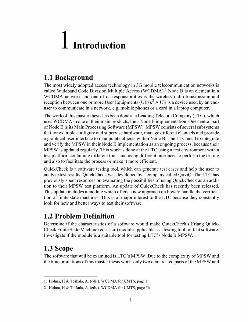
2.1.2 Wideband Code Division Multiple AccessWideband Code Division Multiple Access (WCDMA)4, one of the access technologies found in 3G mobile telecommunication networks was created and developed by 3GPP. WCDMA allows users to communicate with each other in mobile networks. In 2003 this interface was used commercially world wide and is today a standard air interface in 3G mobile telecommunication networks. WCDMA provides support for many different ser-vices simultaneous and uses a bandwidth of 5 MHz.5 Examples of services it supports are voice conversation, video conference and short message service. WCDMA utilizes Code Division Multiple Access (CDMA) technology as its channel access method. It allows many users to use the same frequency at the same time. The WCDMA Radio-Access Network (RAN) architecture is shown in Figure 2-1 on page 4.

3. These groups were: The European Telecommunications Standards Institute, Association of Radio Indus-tries and Business/Telecommunication Technology Committee (ARIB/TTC) (Japan), China Communi-cations Standard Association, Alliance for Telecommunications Industry Solutions (North America) and Telecommunications Technology Association (South Korea)

4. Holma, H & Toskala, A. (eds.). WCDMA for UMTS, page 15. Holma, H & Toskala, A. (eds.). WCDMA for UMTS, page 6

Figure 2-1. WCMA.

4

The WCDMA RAN consists of two types of nodes: Node B and Radio Network Controller (RNC). It is connected to the Core Network (CN), for example Global System for Mobile Communications (GSM), to be able to provide a radio connection to a mobile phone for example.6

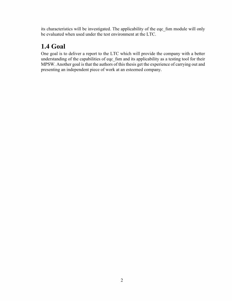
2.1.3 Node B Node B is a an element in a WCDMA network.7 It contains software controlled radio trans-mitters and receivers which it for example uses to communicate with one or several User Equipments (UE) in the network. The UEs can not communicate with other UEs directly, all communication has to pass through a Node B. If two UEs are trying to communicate and they are too far away from each other geographically, more than one Node B has to be used. If this is the case the first UE will make contact with a nearby Node B and if that Node B is unable to reach the second UE, then the Node B will send this information to the RNC. The RNC will then find another Node B located closer to the second UE and communica-tion will be established between the UEs.The MPSW found in the LTC’s Node B implementation have a subsystem called Equip-ment Control (EC). One of EC’s functions is to operate and maintain specific equipment in Node B. EC can for example create and delete different equipment resources in Node B. EC has subsystems of its own and one is called Non Processing Resources (NPR).

6. Ericsson Radio Systems AB. White Paper - Basic Concepts of WCDMA Radio Access Network, page 4 7. Holma, H & Toskala, A. (eds.). WCDMA for UMTS, page 52

Figure 2-2. NPR and EC in Node B.

5

NPR handles the implementation of non-processing resources and one of these resources is called subracks.8 A subrack is a frame where different modules can be mounted. For exam-ple could a mounted module be a fan and its task to regulate the temperature in Node B.

2.1.4 RNCThe RNC is also an element found in a WCDMA network. One or more Node Bs are con-nected to a RNC and the RNC controls the resources of Node B. It is also the service access point for the services WCDMA provides the CN, for example handling the connections to the UEs.9 It is not uncommon that a few hundred Node Bs are connected to a single RNC.10

2.1.5 Transport ChannelsTo be able to transport data between RNCs, Node Bs and UEs special data channels are used. These channels can be grouped in three categories: logical channels, transport chan-nels and physical channels. Logical channels are mapped on transport channels which in turn are mapped on physical channels. A physical channel is defined e.g. by code and fre-quency, while different types of transport channels are defined by how the data is trans-ferred over the air interface and by what characteristics the transferred data has.11 Three types of transport channels are: Forward Access Channel (FACH), Paging Channel (PCH) and Random Access Channel (RACH).12

8. Equipment Control Subsystem Overview, LTC classified document.9. Holma, H & Toskala, A. (eds.). WCDMA for UMTS, page 5310. Dahlman, E., Parkvall, S., Sköld, J. & Beming, P. 3G Evolution HSPA and LTE for Mobile Broadband, page 12911. 3GPP (2009-09), TS 25.211 V8.5.0 - Physical channels and mapping of transport channels onto physi-cal channels (Release 8), page 8 & 9 12. 3GPP (2009-09), TS 25.211 V8.5.0 - Physical channels and mapping of transport channels onto physi-cal channels (Release 8), page 8 & 9

6

2.2 Node B Application Part

Figure 2-3. RNC and Node B signalling via NBAP

The Node B Application Part (NBAP) is the radio network layer signalling protocol used over the Iub13 interface between the RNC and the Node B. NBAP is used e.g. by the RNC to control the resources in Node B or by the Node B to send measurement reports to the RNC. NBAP is defined, developed and updated by the 3GPP. Today NBAP is a standard protocol for carrying signalling traffic between the Node B and the RNC.

2.2.1 Elementary ProceduresNBAP consists of Elementary Procedures (EPs), which is a unit of interaction between the Node B and the RNC. An EP always consists of an initiating message called a request. Sometimes it is also followed by a response message, either a successful response message or an unsuccessful response message. The response message provides detailed information about the outcome of the request.14

There are two types of EPs: common procedures and dedicated procedures.15 Common procedures always have both a request and a response message. A common procedure is first invoked by the RNC and then the common procedure establishes a communication context with a specific UE in the Node B. This communication context contains relevant information for the Node B to be able to communicate with the UE. It is identified by the Node B Communication Context ID. There is an equal RNC communication context and it is identified by the CRNC Communication Context ID. These IDs are necessary to uniquely identify the user, which ensures correct communication between the Node B and the RNC.16

When the Node B Communication Context is established with a specific UE in the Node B, the RNC can send a message to the Node B’s concerned Node B Communication Con-text. If this is done the RNC invokes a dedicated procedure. Their task is to perform mod-ification or removal of resources related to UEs.

13. Iub is explained in Chapter 2.4.14. 3GPP, TS 25.433 version 7.14.0 Release 7 - UTRAN Iub interface Node B Application Part (NBAP) sig-nalling, ETSI TS 125 433 V7.14.0 (2009-10), page 2415. 3GPP, TS 25.433 version 7.14.0 Release 7 - UTRAN Iub interface Node B Application Part (NBAP) sig-nalling, ETSI TS 125 433 V7.14.0 (2009-10), page 3016. 3GPP, TS 25.433 version 7.14.0 Release 7 - UTRAN Iub interface Node B Application Part (NBAP) sig-nalling, ETSI TS 125 433 V7.14.0 (2009-10), page 30

7

2.2.2 Information ElementsA NBAP message can contain a lot of different information and it varies depending on the sender, the receiver and the intention of the message. The intention of the message can for example be either to set up a physical transport channel or just to make a slight change in the same channel. This information is given by the Information Elements (IEs) in the NBAP message.17 There can be several hundred IEs in a message. An IE in a NBAP message is followed by a Presence field. This field is either mandatory, optional or conditional. If the Presence field is mandatory the IE shall always be included in the message, but if it is optional it may or may not be included. If the IE is marked con-ditional, it should be included only if the condition is satisfied.18

2.3 Erlang

2.3.1 HistoryErlang was invented in the mid 80's by researchers at Ericsson's computer science labora-tory. The researchers were looking for a programming language suitable for programming the software of their latest telecom application. At that point, several languages were up for review, including Lisp, Prolog and Parlog.19 The aim was to find something that could be used to develop fault-tolerant, concurrent, distributed, soft real-time systems. None of the existing languages seemed to include all of the features needed to satisfy the researchers’ demands. Influenced by other programming languages e.g. ML and Prolog, they decided to develop a programming language of their own. In 1990 that language was presented and it was called Erlang.20

2.3.2 GeneralErlang is a declarative language, meaning that it describes what should be computed, not how it is calculated. Erlang functions are handled as first class data, which allows them to be bound to variables, stored in data structures or even communicated between different processes.21

Another aspect of Erlang is its process handling. Each process is spawned in its own memory with its own heap and stack. No new threads are created. This makes processes more naturally separated. Also the messaging between processes has some special features. Any kind of data can be sent and the processes can access their mailbox anytime, in any order. These factors contribute to reducing the risk of inadvertent interaction between pro-cesses. Processes will less likely have interaction problems such as deadlocks. 22

17. 3GPP, TS 25.433 version 7.14.0 Release 7 - UTRAN Iub interface Node B Application Part (NBAP) sig-nalling, ETSI TS 125 433 V7.14.0 (2009-10), page 2618. 3GPP, TS 25.433 version 7.14.0 Release 7 - UTRAN Iub interface Node B Application Part (NBAP) sig-nalling, ETSI TS 125 433 V7.14.0 (2009-10), page 20719. History of Erlang, internet source20. Cesarini, F. & Thompson, S. Erlang Programming, page 321. Cesarini, F. & Thompson, S. Erlang Programming, page 4

8

Erlang has mechanisms for error handling and exception monitoring built in its core. One of the mechanisms is the functionality to link processes to each other in order to handle a crashing process and either isolating it or allowing the crash to spread to linked processes. Using these mechanisms as a solid base, general libraries have been written which the Erlang users can use to write robust programs. The programs can be written for the correct case, leaving the error handling to Erlang. This allows programs to be readable, short and contain fewer bugs.23

Communication is a central part of Erlang. Not only does Erlang support interaction with other languages such as C or Java. Erlang was also designed to be suitable for writing pro-grams for distributed systems and for parallel processing. These properties were not added as an afterthought but are inherent in the language design.24

2.3.3 RecordsRecords in Erlang provide a means for the programmer to store a defined number of ele-ments in a data structure, where the elements can be of any type. They share some similar-ities to the structs used in the C language. The user defines the record by specifying exactly what fields it should contain. The initial content of each field can also be specified at dec-laration point or it can be left unspecified. When the content of a field is left unspecified, it simply obtains the atom undefined and can be set to contain any data type later on.Accessing a field in a record is done by using the predefined field name as key, indepen-dently of the structure of the record and the rest of the records fields. This allows the user to add more fields to a record by simply adding them to the record declaration. Any func-tions accessing old fields of that record will remain unaffected by the addition of a new field. 25

2.4 Interfaces

2.4.1 General Node B InterfacesThe Node B has several external interfaces. These interfaces are used to communicate with the Node B. Various interfaces are used depending on the purpose of the communication and who the Node B is communicating with. Different types of communication require access to different types of functionalities in the Node B. There are interfaces for managing the Node B, handling the communication between the Node B and UEs, and for operation and maintenance of the Node B.26

Iub is the interface used between a Node B and an RNC. It is used for traffic related signal-ling. This includes NBAP control signalling, consisting of e.g. transport channel manage-ment including set up and reconfiguring of the transport channels within the Node B.27

22. Cesarini, F. & Thompson, S. Erlang Programming, page 523. Cesarini, F. & Thompson, S. Erlang Programming, page 624. Cesarini, F. & Thompson, S. Erlang Programming, page 825. Cesarini, F. & Thompson, S. Erlang Programming, page 15826. Node B workshop, LTC classified document

9

Mub is the general management interface towards the Node B. It is used for operation and maintenance of the Node B. It can be used either locally at the Node B site via a local area network or from a remote location via CORBA.28

2.4.2 Test EnvironmentThe LTC uses a number of software tools in their test environment in order to test their implementation of the Node B functionality. One of these tools is called Common Test (CT). CT is a library of modules included in Erlang which provides a framework for the user to create and execute tests of an arbitrary System Under Test (SUT)29. CT provides function-ality to communicate with the SUT and execute multiple test cases. The results from these test cases can be logged and presented to the user by CT. Depending on which interface is used to connect to the SUT, CT will use a wrapper module that handles the communication between CT and the SUT via that interface. A number of wrapper modules for target-inde-pendent interfaces are included in CT, e.g. ct_telnet, which handles generic Telnet commu-nication from CT.30

The LTC has created several different module sets which are used in conjunction with CT in order to test the MPSW of their Node B implementation. One of those module sets is called the ct_mo application and it is used to manage communication with a Node B via the Mub interface. The ct_mo application contains a number of modules in order for the user to gain access to different levels of the functionality in the application. One module of inter-est is a ct_mo extension called mub_mo. This module works as a wrapper around ct_mo, aiding the user in accessing the ct_mo functionality. The module will give the user added control over the communication by giving additional control over transitions and increased flexibility in the choice of parameters for functions. The module will also handle return values for the user by trapping exceptions and presenting return values in an informative way, which will aid the user when processing these return values.31

The Bp application is another module set created by the LTC. It is used for communication between the Node B and the test environment at the LTC. The main module in the Bp appli-cation is called bp and includes functionality to handle and communicate a number of pre-defined messages that could be communicated to the Node B.32 Another application in the test environment at the LTC is called the iub application. This application contains several different modules which are designed to aid the testing of dif-ferent areas of functionality of the Node B. One of the modules in the iub application is called nbap.ctcm, where ctcm stands for Common Transport Channel (Configuration)

27. Node B workshop, LTC classified document28. CORBA is an standard protocol used to enable software components typically written in different pro-gramming languages to interact. It is the main protocol for managing a Node B.29. SUT refers to the current partial or complete software system beeing tested for correct operation.30. Common Test Basics, internet source31. The ct_mo application - Mub access, LTC classified document32. The Bp application, LTC classified document

10

Management. This module contains functions which can aid a user who is testing the man-agement and configuration of transport channels in Node B.33

2.5 QuickCheck

2.5.1 BackgroundQuickCheck is a rather new tool for software testing. It was first developed for Haskell in the late 90's, but the industrial Haskell community was quite small. Instead Erlang was growing fast in that circle with 50,000 downloads of Erlang system a month in June 2006.34

Therefore a new version of QuickCheck for Erlang was developed in 2006 by the company QuviQ, which was founded by John Hughes and Thomas Arts the same year.35 Both Hughes and Arts are professors at Chalmers University in Gothenburg, at the Computing Science Department at the department of Applied Information Technology respectively.There are two main aspects that distinguish QuickCheck from other software testing tools. First, QuickCheck tests universally quantified properties of the SUT, rather than single test cases. Based upon these properties, QuickCheck will generate test cases for the user, so he or she does not have to write them one by one. Second, it simplifies test cases showing incorrect beahaviour of the SUT by reducing the complexity of the input data causing the error. I.e. when some input data is found which cause an error in the SUT, QuickCheck will show the user the smallest possible subset of that input data, which will still cause an error in the SUT. This makes it possible for the user to understand the causes of the failures much faster. Together these two features save time and make it possible to find bugs and obscure errors much earlier in the process.Later versions of QuickCheck support model-based testing, by following the structure of finite state machines. This allows for testing of a system by generating sequences of calls to that system. A random sequence of commands can be generated, following a pattern pro-vided by the state machine. The tester might desire e.g. a pattern which mimics the natural behaviour of the SUT.

2.5.2 Symbolic RepresentationIn computer science, a description of data can be used instead of the actual data. This is called symbolic representation. When a program is executed by QuickCheck it uses the actual data, but until then it uses the description of the data, the symbolic representation of the data.QuickCheck uses symbolic representation of test cases, that is, the test is represented as symbolic data and can be manipulated by QuickCheck. In QuickCheck test cases are first generated using symbolic data and after that executed using the actual data. A key in writ-ing models which test cases can be generated from is therefore that all data necessary for creating the test cases need to be present at test generation time.

33. The Iub application, LTC classified document34. Hughes, J. QuickCheck Testing for Fun and Profit.35. Quviq - About us, internet source

11

Here is an example how symbolic representation is done in QuickCheck. When the follow-ing command is executed{set,{var,1},{call,erlang,whereis,[a]}},

it sets variable 1 ({var,1}) to the result of the symbolic function call (where erlang is the module where the function whereis can be found and the parameter a is defined). When the program is executed, or in this case when a test case is run and a symbolic call (call ( )) is performed the symbolic variable (variable 1) is replaced by the value it was set to (the result of whereis with the parameter a). It is important to know that both symbolic calls and vari-ables are used during test generation, but the values they represent are computed during test execution.36

There are three main reasons why QuickCheck uses symbolic representation. First, tests should not depend on a specific representation of a data structure. Second, the process of creating a test result is at least as valuable to know as the result itself. Therefore, the history of obtaining the result should be documented by means of the test case itself. Third, sym-bolic representation helps when one wants to understand and manipulate test data.37 A quote from Hughes, one of the founders of QuickCheck, summarizes the above and adds some additional reasons for the choice of using symbolic representation:

“The reason we chose a symbolic representation is that this makes it easy to print out test cases, store them in files for later use, analyze them to collect statistics or test properties, or – and this is important – write functions to shrink them.”38

2.5.3 SpecificationThe user controls the software testing by writing a QuickCheck specification. A Quick-Check specification consists of a property and one or more generators. The specification tells QuickCheck how to perform the testing by providing information about the properties of the SUT, along with instructions on how input data for the tests should be generated by QuickCheck.

2.5.3.1 PropertiesA common pattern in testing is that the user specifies some input data along with informa-tion about how the SUT is supposed to behave when processing this input data. The user repeats this process and often specifies a large number of pairs of input data and expected results. When the actual testing is performed the input data is fed to the SUT, one by one, and the results are compared to the expected results specified by the user. With QuickCheck this process is different. Instead of asking the user to provide information about how the SUT ought to behave when some specific data is used as input, the user can specify how the SUT should behave in general. The user writes a specification of the properties which ought to hold for the SUT. This naturally demands that the user has some understanding of

36. QuickCheck function index, which is a file included in the QuickCheck distribution.37. QuviQ - QuickCheck for Erlang Users, 2009, page 2238. Hughes, J. QuickCheck Testing for Fun and Profit, page 13

12

how the SUT works. However, a naively written specification of properties would most likely result in errors during testing, which would reveal the glitches in the property speci-fication.By utilizing the functional programming qualities of Erlang, such as macros, QuickCheck allows the user to write manageable and concise properties in a limited number of lines of code. Consider an example where the user wants to verify that the built-in Erlang function lists:delete properly can delete an integer from a list. Using ordinary testing methods, a pro-grammer might write a test suite with several test cases deleting integers from a list and checking if the element was indeed deleted. The programmer might include some lines of code that test borderline cases such as deleting an integer from the empty list or deleting an integer not present in the list. More lines would also be included to test normal cases where the programmer would specify some arbitrary integer to delete from a list containing that integer along with some more arbitrary integers. Testing every possible case in this manner is impossible, but the programmer can add as many cases as he or she likes, by adding more lines of code until he or she feels that adequate test coverage has been reached. Using QuickCheck for the same task, a property specification is used. In this case, the property specification for the SUT can be described in one function. In this example the property function could look like this:prop_lists_delete()

?FORALL(I, int(),

?FORALL(List, list(int()),

not lists:member(I, lists:delete(I,List)))).

This property function says that I is a random integer and List is a list of random length con-taining random integers. If the function lists:delete is called, with the arguments I and List,in an attempt to delete I from L, then the resulting list should not contain I. The property code is written on a form closely related to its corresponding mathematical properties, such as the logical statement:

I int( )∈( ), List list (int( )∈( )· )not(lists:member(I, lists:delete(I,List))

∀∀

This aspect makes QuickCheck properties readable. It also adds value to any formal spec-ification of the SUT by enabling the formal specification to be interpreted as code and adding it to the property specifications without much restructuring of the formal specifica-tion.When a property specification for parts of the SUT or the whole SUT has been constructed, QuickCheck can be instructed to generate input data. Generators are explained in detail in Chapter 2.5.3.2, but in this example QuickCheck would generate arbitrary integers and lists for as many tests as requested. The results of these tests would be compared with the pre-viously specified properties for the SUT in order to tell whether the SUT behaves as expected.39

13

2.5.3.2 GeneratorsQuickCheck provides a means to generate controlled random data to be used as input for test cases. Functions for the generation of basic data types are built in, such as generating random integers, characters or lists. The generator function for e.g. generating a random integer looks like this:int( ).

The generator functions can be combined in order to generate e.g. a list of integers, like this:list(int( )).

The user defines which generators to use for the tests and if the built in generation functions are inadequate, it is possible to write user defined generators. The user is basically free to write generators of any kind including the use of basic generators in Erlang records or with list comprehension, which allows the user to construct complex and powerful generators. The user must however keep in mind that the built in basic generators are not evaluated until runtime. They do not return an instance of the actual data type they are supposed to be generating, but rather a test data generator, which QuickCheck can process when running tests. This means that the user can not simply bind the return value of a generator to a vari-able and use that variable in other functions, assuming those functions expect an instance of the actual data type, rather than the returned test data generator. The use of test data gen-erators is a desired feature of QuickCheck. There are however ways to work around it by using certain provided Erlang macros which can handle the test data generators and provide access to the actual values of the generators.It is the user’s responsibility to define generators that generate well distributed data to be used for the test cases. Consider an example where the user wants to test a system that has a database function which returns some product information given production year, where years are represented as integers. Suppose the database has listed products since the year 2000. The function will then return some information of interest given an integer ranging from 2000 to 2010. The user wants to test this functionality by sending a year integer as input to the system. Testing an odd year integer such as 2099 or -9999 would be interesting a couple of times in order to see if the system responds like it is supposed to when given these abnormal year integers. But in general, testing normal years would be more interest-ing. Simply choosing the built in basic generator for integers, int(), would not generate an integer between 2000 and 2010 often enough, considering how many integers are possible. It is up to the user to write a user defined generator that will result in a better data distribu-tion. There are many ways for the user to define generators. In this case, the user could use the built in generator elements(L) which randomly chooses an element from a list L. The list L could then be hard coded to include integers corresponding to all the possible years from 2000 to 2010, along with a single generator element int(), which would cover the cases of generating years not included in the database.Elements([2000,2001, ... , 2009, 2010, int()]).

39. Hughes, J. QuickCheck Testing for Fun and Profit, and Claessen, Koen and Hughes, John , QuickCheck: A Lightweight Tool for Random Testing of Haskell Programs.

14

The list would contain 11 integers and one generator. Hence a completely random integer would be generated only once in twelve tests, the other eleven cases would be one of the normal years.

2.5.4 ShrinkingQuickCheck generates random sequences of input data for tests. This method is sooner or later prone to find even the most obscure errors that can only be triggered with a particular combination of commands. This is good news. However, that particular combination might be part of a much longer sequence of commands, where most of the commands in that sequence play no part in causing the error. A long sequence of commands can be very dif-ficult to analyze. QuickCheck provides a tool which reduces a long list of commands into a minimal one that still cause an error to occur. This process is called shrinking.The shrinking process is conducted by reducing the size of the error-causing sequence of commands by one or more commands at the time. After each reduction, QuickCheck runs a test with the reduced command sequence. If an error still occurs, QuickCheck will try to remove even more commands. If the reduced sequence no longer produces an error, Quick-Check steps back to a previous state where the command sequence still produced an error. QuickCheck will then try to remove some other command or commands from the sequence. This process is repeated until QuickCheck has fine tuned the command sequence to a min-imal one that still causes the error to occur. This process does not only reduce the number of commands in the sequence but also minimizes other parts included in the sequence. E.g. integers generated in the sequence are reduced to a lower value and strings are cut shorter. The shrinking algorithm uses a greedy search strategy, taking big steps first, in order to find the minimal failing test case. However, should the user prefer it, QuickCheck does provide tools for altering the shrinking process into a different strategy or use no shrinking at all.Hughes says that using a shrinking method in the testing process, could change the eco-nomic perspective of testing.40 Using a test method where test cases are mapped in a one to one fashion between input and results, a limited number of command sequences will be tested. In this way, every failing test case is valuable. Once a failing test case is found, resources will be spent analyzing the command sequence causing the error, no matter how complex that sequence might be. On the other hand, using QuickCheck, generating many test cases is easy. Hence, a found failing command sequence can be thrown away. More test cases can quickly be generated, in hope of finding a less complex command sequence. With the additional support of the shrinking process, once a low complexity command sequence is found, it is likely shrunk to a minimal size. A short, low complexity failing command sequence would need fewer resources to be analyzed. Instead, resources would be spent on constructing a well defined property specification of the SUT, before running the actual tests.41

40. Hughes, J. QuickCheck Testing for Fun and Profit, page 3041. Hughes, J. QuickCheck Testing for Fun and Profit, page 30.

15

2.5.5 Finite State MachinesAn abstract model used for example to model the behavior of a software with a finite number of states and transitions is called a finite state machine. QuickCheck provides two slightly different library modules to test the behavior of such a system: Erlang QuickCheck State Machine (eqc_statem) and a new addition called Erlang QuickCheck Finite State Machine (eqc_fsm).

2.5.5.1 Erlang QuickCheck State MachineTo define a state machine a number of predefined callbacks are written by the QuickCheck user.42 These callbacks let QuickCheck know how the state machine is supposed to behave e.g. what transitions are available and where QuickCheck shall begin traversing the state machine. Many Erlang users are familiar with this idea, since it is often used in open source distribution of Erlang. The basic flow of the state machine and the callback functions used in eqc_statem are shown in Figure 2-4 on page 16. It also shows the test generation phase and the test execu-tion phase with its respective callback functions.

42. A callback consists of executable code that is passed as an argument to other code. This enables a lower level software layer to call a subroutine or function defined in a higher level layer.

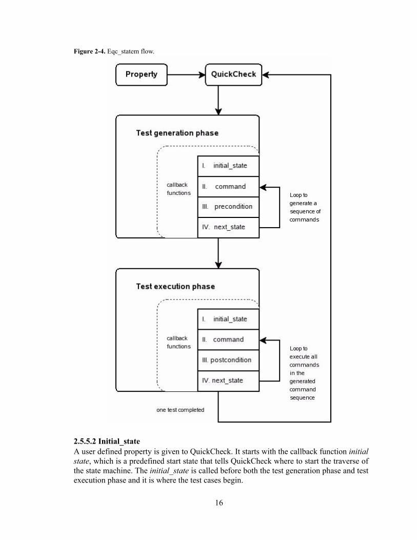
Figure 2-4. Eqc_statem flow.

16

2.5.5.2 Initial_stateA user defined property is given to QuickCheck. It starts with the callback function initial state, which is a predefined start state that tells QuickCheck where to start the traverse of the state machine. The initial_state is called before both the test generation phase and test execution phase and it is where the test cases begin.

17

2.5.5.3 Command The callback function command binds a symbolic variable to the result of a symbolic func-tion call. Command generates one command in each state, which eventually leads to a com-plete generated command sequence. A different function called commands put together the test command sequence, but the callback function command creates the symbolic variables that are included in the sequence:commands( ) generator(list(command( ))).

Each time the command function is called another symbolic variable is added to the test command sequence. This is repeated until it generates the atom stop, which allows com-mand to control the length of the test generated command sequence. This is done in the test generation phase, right after the initial_state function has been called. It is not until the test execution phase that the actual values of the symbolic representations in the test command sequence will be known. The generated commands are however only included in the test command sequence if their preconditions are satisfied.43

2.5.5.4 PreconditionFor each command a separate precondition callback function can be defined. This function is only used during the test generation phase, directly after the command callback function has been called. The precondition function returns a boolean stating if the symbolic call C can be performed in the state S. precondition (S,C) -> bool ( )

If the boolean value is true, the call is added to the test command sequence, otherwise it is excluded. This way commands that contain known errors etc. can be filtered out using pre-conditions, allowing the user to continue testing the SUT without causing the property to fail.One might think that it is unnecessary to define both a command generator and a precon-dition function for each command, since the command generator from the beginning is designed to generate an appropriate command for the current state. Two reasons for doing so are first that the user might write a complex command generator and afterwards wanting to exclude some of them for different reasons, which then is done using a more restrictive precondition. Second, preconditions are needed to assure that the shrinking is correct, because what the shrinking does is that it deletes commands from a test case. This means that a shrunk test case can consist of commands that appear in a different state from where they first were generated in. With preconditions one can determine if the commands are appropriate in the new state or not. Also, preconditions can be used to prevent test cases from testing transitions that have already been found erroneous, enabling the test cases to move on to test other transitions in the state machine.

2.5.5.5 Next_stateThe next_state callback function is used both in the test generation phase and in the test exe-cution phase. In the test generation phase, directly after the precondition function has been called, the next_state function is used to update the changes that the command callback

43. QuickCheck function index, which is a file included in the QuickCheck distribution.

18

function has made to the state. The next_state function has a result parameter, R, and it is symbolic during test generation. During this phase the state could be partly symbolic and partly consist of real values/names. An example of the symbolic representation of the result parameter could be:{var,1}

and the representation of the state in the test generation phase could look like{state,[{a,{var,1}}]}.

Here the a is an actual name and will not be changed during the test execution phase, but the {var,1} will be replaced with the actual values of the symbolic representation during the test execution phase e.g. looking like this: {state,[{a,<0.51>}]}.

In the test execution phase the next_state function will be called right after the postcondi-tion callback function. Next_state will then update the state with the actual values, not the symbolic representation of the values.

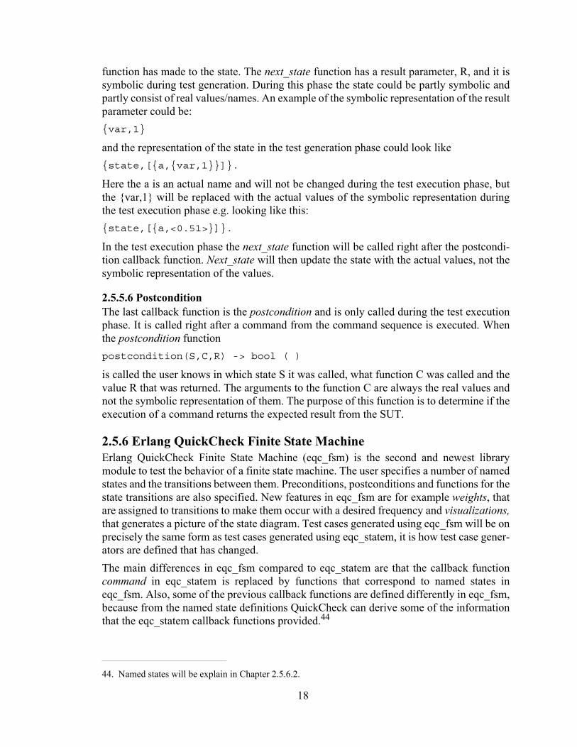
2.5.5.6 PostconditionThe last callback function is the postcondition and is only called during the test execution phase. It is called right after a command from the command sequence is executed. When the postcondition functionpostcondition(S,C,R) -> bool ( )

is called the user knows in which state S it was called, what function C was called and the value R that was returned. The arguments to the function C are always the real values and not the symbolic representation of them. The purpose of this function is to determine if the execution of a command returns the expected result from the SUT.

2.5.6 Erlang QuickCheck Finite State MachineErlang QuickCheck Finite State Machine (eqc_fsm) is the second and newest library module to test the behavior of a finite state machine. The user specifies a number of named states and the transitions between them. Preconditions, postconditions and functions for the state transitions are also specified. New features in eqc_fsm are for example weights, that are assigned to transitions to make them occur with a desired frequency and visualizations,that generates a picture of the state diagram. Test cases generated using eqc_fsm will be on precisely the same form as test cases generated using eqc_statem, it is how test case gener-ators are defined that has changed.The main differences in eqc_fsm compared to eqc_statem are that the callback function command in eqc_statem is replaced by functions that correspond to named states in eqc_fsm. Also, some of the previous callback functions are defined differently in eqc_fsm, because from the named state definitions QuickCheck can derive some of the information that the eqc_statem callback functions provided.44

44. Named states will be explain in Chapter 2.5.6.2.

19

2.5.6.1 Goals with Eqc_fsmIt was important for the developers that eqc_fsm looked and felt similar to eqc_statem, because they wanted QuickCheck's current users to easily adapt and understand the changes that had been made. Other goals when constructing eqc_fsm was to concisely spec-ify the information in a state diagram only once. It was also desirable to separate the state into a state name and state data. Another goal with eqc_fsm was to reduce the gap between the code and the state machine diagram. The finite state machine modeled by eqc_statem can be considered to be a server, the state is encapsulated in the data, but all events may arrive at any time. The finite state machine extension eqc_fsm limits the possibility to events that can only happen in a certain state. Since the state is more explicit in eqc_fsm than in eqc_statem, the state data is also more explicit and the model needs to consider both parts in the callback functions.

2.5.6.2 The ChangesState Names and State DataCompared to eqc_statem, eqc_fsm splits the state into two parts: a state name and state data. The state name represents one of the states in the finite state machine. The state data can include any relevant information the user wants to store in the state and the state data is usu-ally an Erlang record. When a state is completed it is represented by its state name and its state data as a pair:{state_name, {state_data}}.

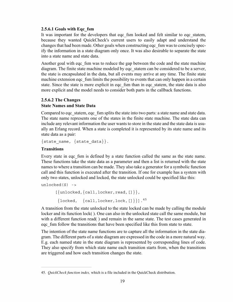
TransitionsEvery state in eqc_fsm is defined by a state function called the same as the state name. These functions take the state data as a parameter and then a list is returned with the state names to where a transition can be made. They also take a generator for a symbolic function call and this function is executed after the transition. If one for example has a system with only two states, unlocked and locked, the state unlocked could be specified like this:unlocked(S) ->

[{unlocked,{call,locker,read,[]}},

{locked, {call,locker,lock,[]}}].45

A transition from the state unlocked to the state locked can be made by calling the module locker and its function lock( ). One can also in the unlocked state call the same module, but with a different function read( ) and remain in the same state. The test cases generated in eqc_fsm follow the transitions that have been specified like this from state to state. The intention of the state name functions are to capture all the information in the state dia-gram. The different parts of a state diagram are expressed in the code in a more natural way. E.g. each named state in the state diagram is represented by corresponding lines of code. They also specify from which state name each transition starts from, when the transitions are triggered and how each transition changes the state.

45. QuickCheck function index, which is a file included in the QuickCheck distribution.

20

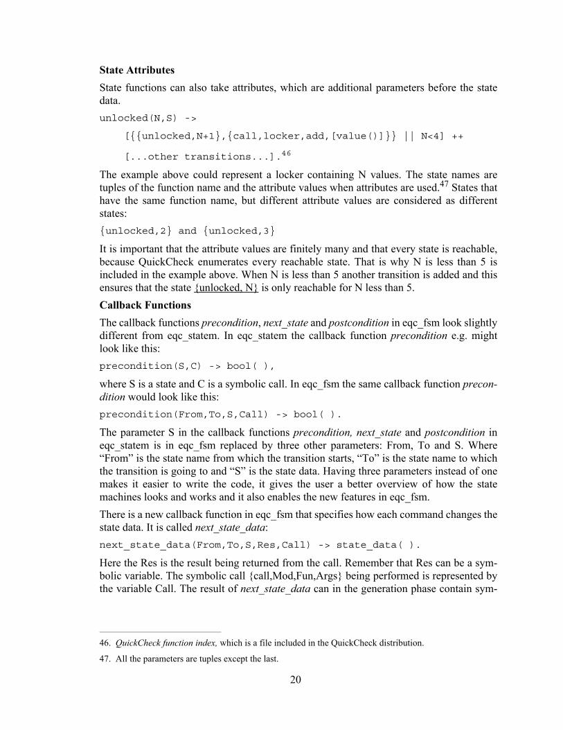
State AttributesState functions can also take attributes, which are additional parameters before the state data. unlocked(N,S) ->

[{{unlocked,N+1},{call,locker,add,[value()]}} || N<4] ++

[...other transitions...].46

The example above could represent a locker containing N values. The state names are tuples of the function name and the attribute values when attributes are used.47 States that have the same function name, but different attribute values are considered as different states:{unlocked,2} and {unlocked,3}

It is important that the attribute values are finitely many and that every state is reachable, because QuickCheck enumerates every reachable state. That is why N is less than 5 is included in the example above. When N is less than 5 another transition is added and this ensures that the state {unlocked, N} is only reachable for N less than 5.Callback FunctionsThe callback functions precondition, next_state and postcondition in eqc_fsm look slightly different from eqc_statem. In eqc_statem the callback function precondition e.g. might look like this:precondition(S,C) -> bool( ),

where S is a state and C is a symbolic call. In eqc_fsm the same callback function precon-dition would look like this: precondition(From,To,S,Call) -> bool( ).

The parameter S in the callback functions precondition, next_state and postcondition in eqc_statem is in eqc_fsm replaced by three other parameters: From, To and S. Where “From” is the state name from which the transition starts, “To” is the state name to which the transition is going to and “S” is the state data. Having three parameters instead of one makes it easier to write the code, it gives the user a better overview of how the state machines looks and works and it also enables the new features in eqc_fsm.There is a new callback function in eqc_fsm that specifies how each command changes the state data. It is called next_state_data:next_state_data(From,To,S,Res,Call) -> state_data( ).

Here the Res is the result being returned from the call. Remember that Res can be a sym-bolic variable. The symbolic call {call,Mod,Fun,Args} being performed is represented by the variable Call. The result of next_state_data can in the generation phase contain sym-

46. QuickCheck function index, which is a file included in the QuickCheck distribution.

47. All the parameters are tuples except the last.

21

bolic variables and function calls, just as next_state can in eqc_statem. These symbolic variables are replaced by their actual values in the test execution phase. Initial State Normally each test case starts in the same initial state. Two callback functions specify the initial state:initial_state( ) and initial_state_data( ).

The callback function initial_state( ) allows the user to specify where to start in the state machine, and the function initial_state_data( ) allows the user to specify what the state data should contain initially.

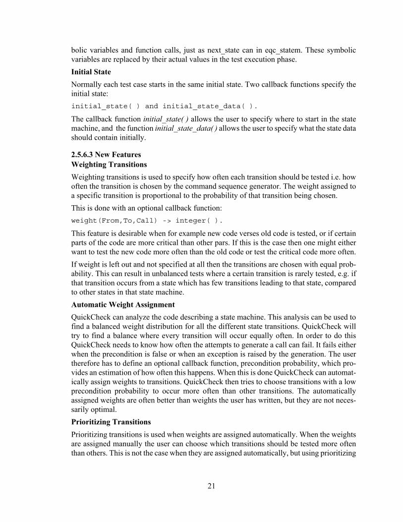
2.5.6.3 New FeaturesWeighting TransitionsWeighting transitions is used to specify how often each transition should be tested i.e. how often the transition is chosen by the command sequence generator. The weight assigned to a specific transition is proportional to the probability of that transition being chosen.This is done with an optional callback function:weight(From,To,Call) -> integer( ).

This feature is desirable when for example new code verses old code is tested, or if certain parts of the code are more critical than other pars. If this is the case then one might either want to test the new code more often than the old code or test the critical code more often.If weight is left out and not specified at all then the transitions are chosen with equal prob-ability. This can result in unbalanced tests where a certain transition is rarely tested, e.g. if that transition occurs from a state which has few transitions leading to that state, compared to other states in that state machine.Automatic Weight AssignmentQuickCheck can analyze the code describing a state machine. This analysis can be used to find a balanced weight distribution for all the different state transitions. QuickCheck will try to find a balance where every transition will occur equally often. In order to do this QuickCheck needs to know how often the attempts to generate a call can fail. It fails either when the precondition is false or when an exception is raised by the generation. The user therefore has to define an optional callback function, precondition probability, which pro-vides an estimation of how often this happens. When this is done QuickCheck can automat-ically assign weights to transitions. QuickCheck then tries to choose transitions with a low precondition probability to occur more often than other transitions. The automatically assigned weights are often better than weights the user has written, but they are not neces-sarily optimal.Prioritizing TransitionsPrioritizing transitions is used when weights are assigned automatically. When the weights are assigned manually the user can choose which transitions should be tested more often than others. This is not the case when they are assigned automatically, but using prioritizing

22

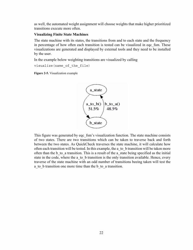
as well, the automated weight assignment will choose weights that make higher prioritized transitions execute more often. Visualizing Finite State Machines The state machine with its states, the transitions from and to each state and the frequency in percentage of how often each transition is tested can be visualized in eqc_fsm. These visualizations are generated and displayed by external tools and they need to be installed by the user.

Figure 2-5. Visualization example

In the example below weighting transitions are visualized by callingvisualize(name_of_the_file)

This figure was generated by eqc_fsm’s visualization function. The state machine consists of two states. There are two transitions which can be taken to traverse back and forth between the two states. As QuickCheck traverses the state machine, it will calculate how often each transition will be tested. In this example, the a_to_b transition will be taken more often than the b_to_a transition. This is a result of the a_state being specified as the initial state in the code, where the a_to_b transition is the only transition available. Hence, every traverse of the state machine with an odd number of transitions beeing taken will test the a_to_b transition one more time than the b_to_a transition.

23

3Previous Work

A few master’s theses about QuickCheck have been written in the past. Two of them are called "NBAP message construction using QuickCheck" and "Testing a radiotherapy sup-port system with QuickCheck". These master theses did not have much in common except that QuickCheck was the foundation in both of them and that the results of the theses were of interest to the companies where they were written.

3.1 NBAP Message Construction Using QuickCheckAt Ericsson where the master thesis "NBAP message construction using QuickCheck" was done, the MPSW in Node Bs was tested using scripted regression test case suites.48 The test cases were designed on the basis of use cases and functional specifications. This often results in one-to-one test cases which makes it almost impossible to reuse the code. It also makes it hard to maintain the scripted regression test case suites and furthermore the test suites get very repetitive.49

3.1.1 PurposeOne of the purposes with the "NBAP message construction using QuickCheck" was to examine if it was possible to model the SUT better with QuickCheck and if it was possible to automate much of the test cases used to test the MPSW in Node B with QuickCheck. The idea was to make QuickCheck automatically generate the EPs in a NBAP message. Then maybe QuickCheck could find a broader variety of the EPs to test, which hopefully could result in finding faults that could not be found prior using QuickCheck.50

3.1.2 TaskThe main task was to use QuickCheck to implement test cases for a subset of the MPSW functionality and then integrate these test cases into the company’s test framework. The intention was to enable for a spreading of QuickCheck in the company’s testing framework in the future.

48. Scripted regression test case suites are used in a testing technique where a number of predefined suites containing test cases are scripted to run on schedule, testing the same test cases every time, looking for errors caused by updates on the system under test.49. Granberg, A. & Jernberg, D. NBAP message constructing using QuickCheck, page 1 & 1750. Granberg, A. & Jernberg, D. NBAP message constructing using QuickCheck, page 1

24

3.1.3 ImplementationSince there are many EPs in a NBAP message it was not possible to make QuickCheck automatically generate all of them. It was decided to implement five EPs in a functionality referred to as RLM in MPSW. The SUT, the RLM functionality in the Node B, was mod-eled as state machines using eqc_statem in QuickCheck. Then with simple test cases that invoked a state machine to run QuickCheck was integrated into the framework.

3.1.4 ConclusionQuickCheck could produce the same tests as conventional testing. It could test the same functionality over and over again, but it could also produce many variations of the same test cases and then be able to find faults that scripted test cases could miss. Test cases written in the conventional manner consists of much more code than test cases written for QuickCheck. Using QuickCheck to write test cases would save time and the code would also be much easier to maintain since the code is shorter.

3.2 Testing a Radiotherapy Support System With QuickCheckThis master thesis was performed at a medical company in Sweden. They had developed a position tracking device called the Four Dimension Radio Therapy (4DRT), which was optimized for the human body and also a real-time organ position tracking system. What it did was that it e.g. gave the position of an organ in four dimensions.51 When cancer patients need radiation 4DRT is used to monitor the position of the tumor and helps to improve the accuracy during radiotherapy treatments. The estimated position of an organ is calculated by a mathematical model in the system and should guarantee that the estimated position is close enough to the real position.52

3.2.1 PurposeThe purpose of the master thesis "Testing a radiotherapy support system with QuickCheck" was to test the implementation of the 4DRT, since there could be differences between the model and the actual implementation.53

3.2.2 TaskThe task was to use QuickCheck to make sure that the system in the 4DRT estimated a posi-tion of the organ that was within a radial distance of 2 millimeters from the actual position. Otherwise healthy tissue around the tumor would be damaged and the tumor might not receive the radiation it needs to disappear.54

51. Yamashita, A. & Bergqvist, A. Testing a radiotherapy support system with QuickCheck, page 752. Yamashita, A. & Bergqvist, A. Testing a radiotherapy support system with QuickCheck, page 853. Yamashita, A. & Bergqvist, A. Testing a radiotherapy support system with QuickCheck, page 6 & 754. Yamashita, A. & Bergqvist, A. Testing a radiotherapy support system with QuickCheck, page 8

25

3.2.3 ImplementationThe mathematical model in the system that estimated the position of an organ used a coor-dinate system, and this system was specified as a model. QuickCheck then generated thou-sands of automated test cases based upon that model.55

3.2.4 ConclusionThe model and the implementation of the 4DRT corresponded well, but a number of errors were found in code for the 4DRT. These errors were corrected and resulted in the 4DRT being a higher quality product than it was before. It was simple to write the QuickCheck model, it was clear and based on a mathematical model. Therefore the authors believe that more medical equipment should be tested using QuickCheck.56

3.3 A Comparison With Two Master Theses Using QuickCheckLike the thesis “NBAP message construction using QuickCheck", the present thesis describes testing of a subset of the MPSW functionality. The testing was done by modelling the SUT as finite state machines using QuickCheck. The difference is that "NBAP message construction using QuickCheck" modeled the SUT using eqc_statem in QuickCheck while this master thesis will use the newer eqc_fsm module. A large part of the "NBAP message construction using QuickCheck" thesis focused on the EPs in a NBAP message, while the NBAP messages in this thesis are more or less seen as a means to accomplish the mission of the master thesis. Further more, this thesis is about finding the characteristics of a soft-ware which would make the same software suitable to model and test using eqc_fsm in QuickCheck. While "NBAP message construction using QuickCheck" was more about implementing and integrating test cases. The purpose of the "Testing a radiotherapy support system with QuickCheck" thesis was to examine if there were any differences between the model of the device 4DRT and the actual implementation of it. This is something that this thesis could check too, indirectly, since the function specifications are used to create the state machines in QuickCheck. Then the real implementation of the SUT in the Node B will be tested and if there were any differences between the function specifications and the real implementation of the SUT it would hope-fully be detected. Both the master theses "NBAP message construction using QuickCheck" and "Testing a radiotherapy support system with QuickCheck" concluded that QuickCheck was a very good testing tool, helping to solve many different matters.

55. Yamashita, A. & Bergqvist, A. Testing a radiotherapy support system with QuickCheck, page 6 & 956. Yamashita, A. & Bergqvist, A. Testing a radiotherapy support system with QuickCheck, page 20

26

27

4Methodology

4.1 Literature studies

4.1.1 QuickCheck Course for Erlang UsersA three day QuickCheck course held by the founders of QuickCheck Hughes and Arts was attended. Lectures were followed by exercises so that the new knowledge was used, improved and remembered. Course material was handed out during the course, and used throughout the work of this thesis.

4.1.2 QuickCheck LiteratureRelevant literature was gathered about QuickCheck. Apart from the course material from the QuickCheck course, an interview with Hughes by Sadek Drobi on Nov. 05, 2009 was listened to.57 Articles read about QuickCheck were the following: QuickCheck: A Light-weight Tool for Random Testing of Haskell Programs 58, Finding Race Conditions in Erlang with QuickCheck and PULSE 59 and QuickCheck Testing for Fun and Profit 60. A function description of QuickCheck and all of its modules etc. was also read.

4.1.3 Erlang Basic CourseAn Erlang basic course was carried out since Erlang was the programming language used in QuickCheck. The course was divided into self studies, where one read about Erlang, and exercises, where the obtained information was used and tested. After this course was fin-ished the basics of Erlang programming was learnt.

4.1.4 Network ArchitectureTo get a better overview of how to solve the problem definition, more knowledge about WCDMA, Node B and RNC was needed. This information was gathered by reading confi-dential documents at the LTC, relevant Internet pages and the following books: WCDMA for UMTS61 and 3G Evolution HSPA and LTE for Mobile Broadband62.

57. InfoQ, internet source58. Claessen, Koen and Hughes, John (2000), QuickCheck: A Lightweight Tool for Random Testing of Haskell Programs, internet source.59. Claessen, Koen, Palka, Michal, Smallbone, Nicholas, Hughes, John, Svensson, Hans, Arts, Thomas and Wiger, Ulf (2009), Finding Race Conditions in Erlang with QuickCheck and PULSE, internet source.60. Hughes, John (2007), QuickCheck Testing for Fun and Profit.61. Holma, H & Toskala, A. (eds.)ohn (2001). WCDMA for UMTS.62. Dahlman, E., Parkvall, S., Sköld, J. & Beming, P. 3G Evolution HSPA and LTE for Mobile Broadband.

28

4.1.5 NBAPThe technical specification of NBAP was studied.63 This was done to get knowledge of the structure of the NBAP messages, its parameters and its functions and also to get knowledge of when to use different NBAP messages.

4.1.6 Interfaces and Applications Two external Node B interfaces were important to recognize and know more about: Iub and Mub. The LTC use a software tool in their test environment in order to test their implemen-tation of the Node B functionality called Common Test. The LTC had created different applications to use in conjunction with Common Test: ct_mo application, bp_applicationand iub_application.To get the knowledge to understand the interfaces and applications just mentioned, infor-mation was gathered from Internet pages, technical specifications and internal LTC docu-ments.

4.2 Practical Work

4.2.1 Testing at LTC, General StudiesMuch knowledge has been gained from looking into the LTC’s files and documentation. The knowledge gained was about the LTC’s Node B and RNC implementations, their dif-ferent test suites, platforms and tools used at the LTC.

4.2.2 Manual Testing at LTCThe Node B had to be configured right before starting QuickCheck tests. To come up with the right configuration, documents were read combined with some valuable tip-offs from our supervisor.A lot of manual testing was done on how to send various messages including NBAP mes-sages from Erlang via the Mub and Iub interfaces to the Node B. When this was achieved time was spent on sending different signals to the Node B. Signals sent were for example a signal telling the Node B to set up a subrack.

4.2.3 SUTWhich two systems to test in LTC’s MPSW was decided together with our supervisor. The documentation and the specifications about the two selected systems were carefully read and investigated. Also, the systems models were studied. Then, on a white board, the sys-tems were modelled by hand as state machines.

4.2.4 Running QuickCheckThe systems modelled by hand were transferred to code according to eqc_fsm, which was used to test the SUTs using QuickCheck. The test results were then documented.

63. 3GPP (2009-10), UTRAN Iub interface Node B Application Part (NBAP) signalling, ETSI TS 125 433 V7.14.0

29

5Technical Solution

Two demarcated parts of the LTC’s MPSW, two subsystems, were modelled as finite state machines and tested using QuickCheck. There were several reasons for choosing these two particular systems. The systems were expected to lack complex interactions and to be small enough, allowing complete tests of the systems to be designed and executed within the desired timeframe. Also, the supervisors had some knowledge about the two systems, which allowed them to provide proper guidance when needed. The first system to be modelled and tested was a demarcated part of the NPR, located in MPSW’s EC in the Node B. This first part contains functionality to handle the subrack resources in Node B. This functionality can be triggered by sending signals to the Node B via the Mub interface, and the Node B returns a response message via the same interface. The second system handles transport channels. This part contains functionality which can be triggered by sending NBAP messages to the Node B via the Iub interface, and the Node B returns a response message via the same interface.A third, fictive system was modelled. This system is not part of any system at the LTC. It was designed in order to test a system with characteristics which differ from those found in the two systems investigated in practice. The characteristics of these systems were investigated in order to determine if Quick-Check's eqc_fsm module is applicable as a testing tool for MPSW and also to determine if eqc_fsm is a suitable tool for testing the Node B software.

5.1 Equipment Control

5.1.1 SUT DescriptionThe first SUT chosen to be modeled and tested was a part of NPR, which is a secluded part within EC. The NPR handles the implementation of non-processing resources. This includes the functionality to handle the subracks in the Node B. The first SUT was a part of the NPR functionality, demarcated to only include the functionality to set up and release subracks. This functionality was accessed externally via the Mub interface. This allowed for testing to be performed without taking account for any interactions and dependencies that the SUT had with other parts of the Node B. The start state of the model was decided to be a state of the Node B where no subracks have been set up, but the Node B is prepared to accept requests to set up new subracks. At this point, the Node B is in an idle state waiting for incoming requests. Requests can be sent at any time to set up subracks. Once a subrack is set up, it obtains an identification number. Using this number, the specific subrack can be released at any time.

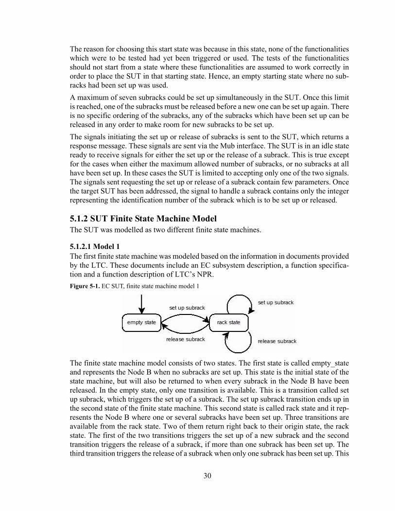
30

The reason for choosing this start state was because in this state, none of the functionalities which were to be tested had yet been triggered or used. The tests of the functionalities should not start from a state where these functionalities are assumed to work correctly in order to place the SUT in that starting state. Hence, an empty starting state where no sub-racks had been set up was used.A maximum of seven subracks could be set up simultaneously in the SUT. Once this limit is reached, one of the subracks must be released before a new one can be set up again. There is no specific ordering of the subracks, any of the subracks which have been set up can be released in any order to make room for new subracks to be set up. The signals initiating the set up or release of subracks is sent to the SUT, which returns a response message. These signals are sent via the Mub interface. The SUT is in an idle state ready to receive signals for either the set up or the release of a subrack. This is true except for the cases when either the maximum allowed number of subracks, or no subracks at all have been set up. In these cases the SUT is limited to accepting only one of the two signals. The signals sent requesting the set up or release of a subrack contain few parameters. Once the target SUT has been addressed, the signal to handle a subrack contains only the integer representing the identification number of the subrack which is to be set up or released.

5.1.2 SUT Finite State Machine ModelThe SUT was modelled as two different finite state machines.

5.1.2.1 Model 1

Figure 5-1. EC SUT, finite state machine model 1

The first finite state machine was modeled based on the information in documents provided by the LTC. These documents include an EC subsystem description, a function specifica-tion and a function description of LTC’s NPR.

The finite state machine model consists of two states. The first state is called empty_state and represents the Node B when no subracks are set up. This state is the initial state of the state machine, but will also be returned to when every subrack in the Node B have been released. In the empty state, only one transition is available. This is a transition called set up subrack, which triggers the set up of a subrack. The set up subrack transition ends up in the second state of the finite state machine. This second state is called rack state and it rep-resents the Node B where one or several subracks have been set up. Three transitions are available from the rack state. Two of them return right back to their origin state, the rack state. The first of the two transitions triggers the set up of a new subrack and the second transition triggers the release of a subrack, if more than one subrack has been set up. The third transition triggers the release of a subrack when only one subrack has been set up. This

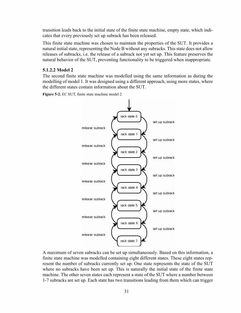
31

transition leads back to the initial state of the finite state machine, empty state, which indi-cates that every previously set up subrack has been released.This finite state machine was chosen to maintain the properties of the SUT. It provides a natural initial state, representing the Node B without any subracks. This state does not allow releases of subracks, i.e. the release of a subrack not yet set up. This feature preserves the natural behavior of the SUT, preventing functionality to be triggered when inappropriate.

5.1.2.2 Model 2

Figure 5-2. EC SUT, finite state machine model 2

The second finite state machine was modelled using the same information as during the modelling of model 1. It was designed using a different approach, using more states, where the different states contain information about the SUT.

A maximum of seven subracks can be set up simultaneously. Based on this information, a finite state machine was modelled containing eight different states. These eight states rep-resent the number of subracks currently set up. One state represents the state of the SUT where no subracks have been set up. This is naturally the initial state of the finite state machine. The other seven states each represent a state of the SUT where a number between 1-7 subracks are set up. Each state has two transitions leading from them which can trigger

32

the set up or the release of a subrack. This is true except for two cases. First, the release of subracks is not allowed in the state where no subracks have been set up. Second, the set up of subracks is not allowed when the maximum number of subracks already has been set up.The choice of using separate states for every possible number of subracks set up offers pre-cise control of which transitions to allow in each state and where they should end up. It also allows the state machine itself to directly reveal information about the SUT and its proper-ties, just by looking at what state the SUT is at in the state machine.

5.1.3 QuickCheck ImplementationThe finite state machine models were to be converted to Erlang code according to Quick-Check’s eqc_fsm behavioural model. The purpose of this code was to use the eqc_fsm module and implement QuickCheck tests covering the functionality of the chosen SUT.

5.1.3.1 Model 1The two states of the first Equipment Control SUT model were each represented in the Erlang code as a QuickCheck callback function. These callback functions return a list of possible transitions from that state. This information is used by eqc_fsm to determine how to traverse the state machine. QuickCheck’s automated weight assignment was used to bal-ance QuickCheck’s traverses of the state machine. With each transition, a matching func-tion is called which tests a part of the SUT’s functionality. These functions simulate the act of sending a signal to the SUT. The signals are sent via the Mub interface, using the mub_mo wrapper module of the ct_mo application. Using the mub_mo module, response messages will be presented from the SUT. These response mes-sages are handled by eqc_fsm’s postcondition callback function, where the responses are analyzed to confirm that the SUT responds according to its specification.As eqc_fsm traverses the state machine, an Erlang record, containing state data is passed on from state to state. This record is used both to keep track of the number of subracks cur-rently set up and the subracks’ identification numbers. This data is stored in a list in the record. At this point, a single list would be sufficient for to store this data. However, placing the list in a record makes the code flexible as the record easily could be expanded to include additional data of different types if needed. Using this record, the tests were configured in two ways. The first configuration used eqc_fsm’s precondition callback function to prevent any attempts to set up subracks, if the record stated that the maximum subracks had already been reached. The second configuration allowed attempts to set up subracks at any time. This time the postcondition function was configured to analyze a negative response mes-sage as a positive test result, when the record stated that the maximum amount of subracks already had been set up. The subrack set up signals sent to the SUT specifies the identification number of the sub-rack. This number was chosen randomly using a QuickCheck generator covering a defined interval of integers. When a subrack has been successfully set up, its corresponding identi-fication number is stored in the state data Erlang record. This information is later used in two ways. First, when releasing subracks, only previously set up subracks are targeted using the identification numbers from the record. Second, an attempt to set up a subrack using an identification number used in an already set up subrack will result in an error

33

response message from the SUT. This message will be analyzed by the postcondition func-tion as a successful test given that the identification number is included in the state data record.

Figure 5-3. EC SUT, finite state machine model 1, generated by eqc_fsm.

This implementation covers the SUT’s functionality by analyzing its response messages when given a signal to manage the subracks, making sure the response messages follow the specification of the SUT. It does not however, check the SUT’s actual condition with its internal representation of the subracks.

Figure 5-3 was generated using eqc_fsm’s visualize function. Eqc_fsm uses the Erlang code implementation of the SUT finite state machine to generate the figure. The numbers next to each transition display how often that particular transition was traversed, as a per-centage of the total number of transitions traversed. These particular numbers were obtained using QuickCheck’s automated weight assignment.

5.1.3.2 Model 2The eight states of the second model are similar in their properties and behaviour, espe-cially the six states representing everything but the states with the maximum or the mini-mum number of subracks. The eight states were represented in Erlang code as a single QuickCheck state callback function. Using a part of the state name as a variable allowed all the states to be combined into one callback function with four constraints determining what transitions were allowed from the different states. QuickCheck’s automated weight assignment was used to balance QuickCheck’s traverse of the state machine. At every transition, a function was called which tests some part of the SUT functionality.As in model 1, these functions send signals to the SUT using mub_mo and the response messages are handled by the postcondition callback function, which confirms that the SUT responds according to its specification. Model 2 uses an Erlang record to preserve data about previous transitions. This record is passed on from state to state as QuickCheck traverses the state machine. Every set up sub-rack is given an identification number, a random integer generated from a specified inter-val. The Erlang record keeps track of the identification numbers of all the subracks

34

currently set up. Like in model 1, the record is used to let QuickCheck know that response messages containing errors are to be expected in two cases. First, if an attempt is made to release a subrack with a specific identification number which is not stored in the record. Second, if an attempt is made to set up a subrack with a specific identification number which is already stored in the record. The QuickCheck tests were configured in two differ-ent ways with the use of this information. First, eqc_fsm’s precondition callback function was used to make sure that no functions were called from a transition where the return mes-sage was expected to be negative. The second approach tested was to allow any type of tran-sition, but if the return message was negative, it would still be considered a passed test if the information in the record indicated that a negative result was expected. Likewise, a pos-itive result in this case would be considered a failed test.Eqc_fsm’s automatic weight assignment function was used to find values which were used in eqc_fsm’s weight callback functions to balance the times every transition in each of the eight states were taken.

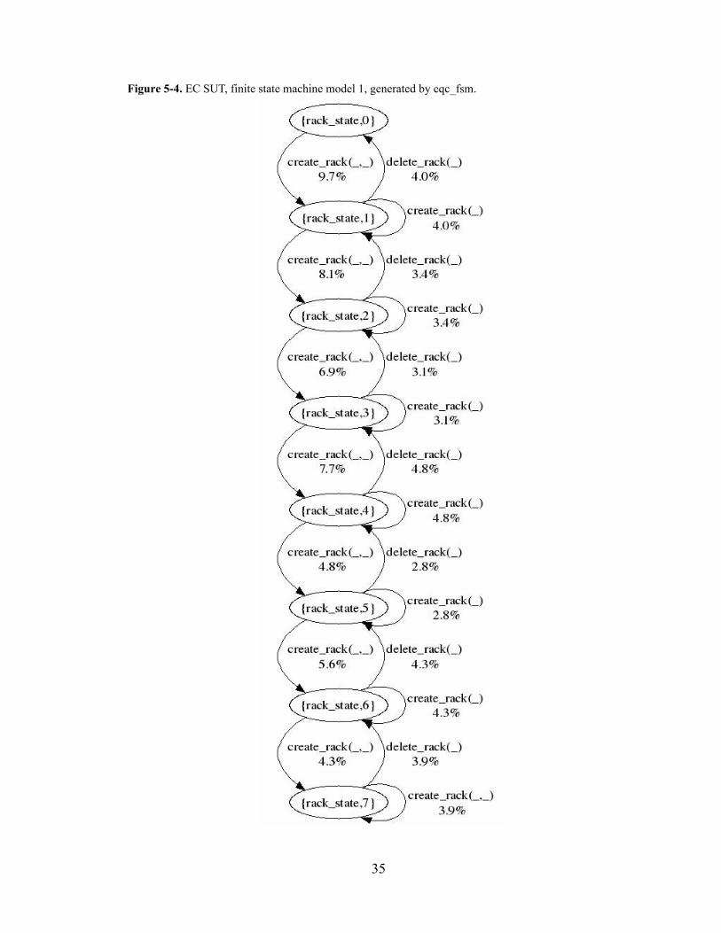
Figure 5-4. EC SUT, finite state machine model 1, generated by eqc_fsm.

35

36

Figure 5-4 was generated using eqc_fsm’s visualize function. Eqc_fsm uses the Erlang code implementation of the SUT finite state machine to generate the figure. The numbers next to each transition display how often that particular transition was taken, as a percent-age of the total number of transitions taken. These particular numbers were obtained using QuickCheck’s automated weight assignment.

5.1.4 ResultsQuickCheck tests were run continuously throughout the implementation process. When new code was written and integrated in the QuickCheck test code, it was tested right away using QuickCheck. This means that a lot of tests were completed using early versions of the code or semi-completed code. These tests were not documented.Once the code was completed, a number of tests were executed and timed. For each of the two models, four sets of QuickCheck tests were completed. The four sets execute a total of 13,000 test cases, traversing the finite state machines generating 13,000 sequences of com-mands calling functions which test the SUT’s functionality. The tests were completed in three sets of 1,000 tests each and one set of 10,000 tests. Execution times of the tests were recorded and the maximum and average command sequence lengths were computed. Results of the tests are presented in Table 5-1 and Table 5-2.

Table 5-1. EC Model 1, test resultsSet 1,000 1,000 1,000 10,000

Execution Time (minutes) 8.7 8.5 8.4 87.3

Maximum sequence length 134 116 141 216

Average sequence length 15.7 15.3 15.1 15.8

SUT errors found 0 0 0 0

Table 5-2. EC Model 2, test resultsSet 1,000 1,000 1,000 10,000

Execution Time (minutes) 8.8 8.9 8.7 90.4

Maximum sequence length 153 116 145 205

Average sequence length 16.2 16.6 15.9 16.0

SUT errors found 0 0 0 0

The source lines of code of the Erlang code was counted, excluding blank lines and is pre-sented in Table 5-3.

Table 5-3. EC SUT source lines of codeModel 1 Model 2

Comment 18 16

Code 112 124

Total 130 140

37

The Erlang code for the two models was written by the authors, working together for 16 days spread out over a 30 day period. Out of these 16 days of work, 5 days of work were oriented mainly towards implementing the QuickCheck-specific parts of the code, while the other 11 days of work were oriented mainly towards implementing the Erlang functions communicating with the SUT.

5.2 Transport Channels

5.2.1 SUT DescriptionThe second SUT to be tested was a demarcated part of the Node B which handles the set up, release and reconfiguration of the transport channels FACH, PCH and RACH. The SUT includes functionality to set up one PCH and/or one RACH and/or a pair of FACHs. The SUT also contains functionality to specifically release any of the set up transport channels. A PCH which has been set up can be reconfigured by altering the power value of the chan-nel. A maximum of one PCH, one RACH and a pair of FACHs can be set up simultane-ously. All of the functionality is triggered by NBAP messages sent via the iub interface. After the functionality requested in the NBAP message is executed, the SUT sends a NBAP response message back via the iub interface. Before testing, the SUT was configured to a state where it accepts incoming NBAP mes-sages and where it is possible to set up transport channels. No channels were set up when the testing began.

5.2.2 SUT Finite State Machine Model

5.2.2.1 Model 1The first model was designed using an approach where every possible combination oftransport channels had a different state. This means that for the three different types of channels, PCH, FACH and RACH, there are eight different combinations, hence the model was designed using those eight states. The initial state of the finite state machine is the state where no transport channels have been set up.

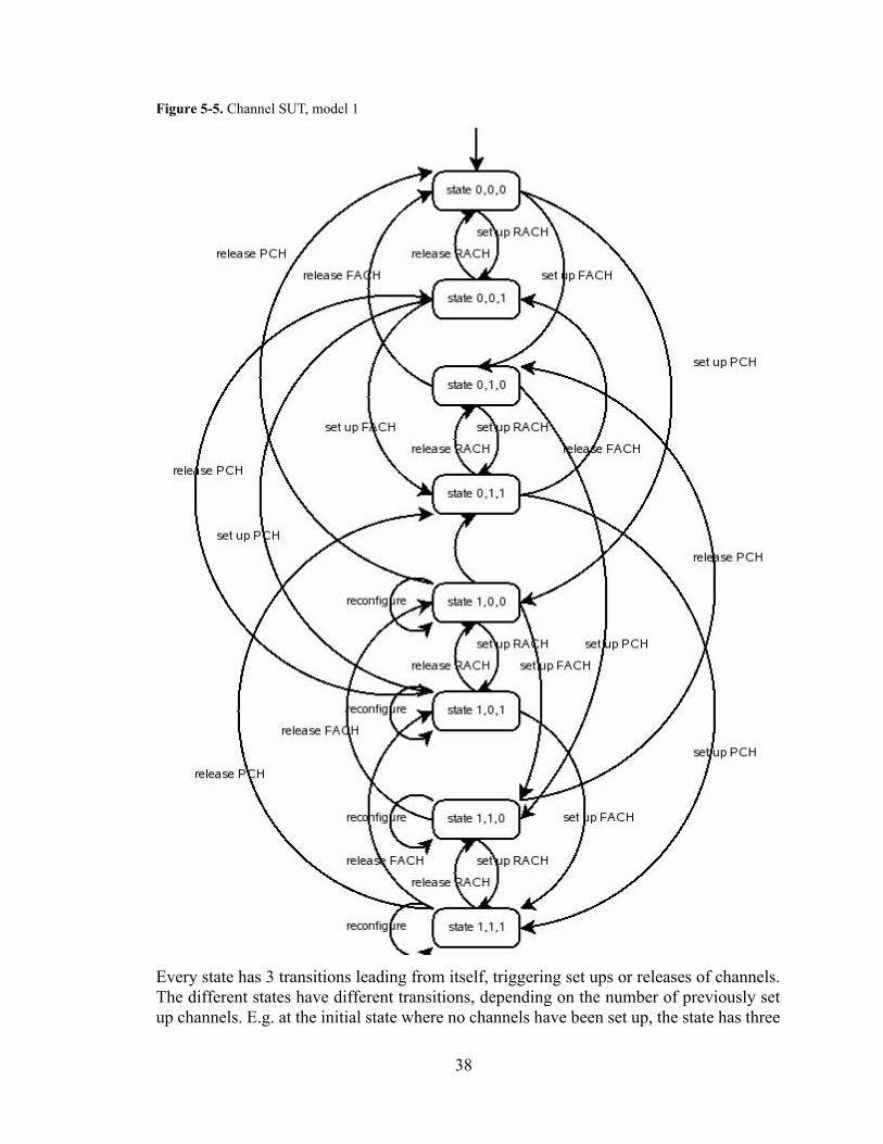
Figure 5-5. Channel SUT, model 1

38

Every state has 3 transitions leading from itself, triggering set ups or releases of channels. The different states have different transitions, depending on the number of previously set up channels. E.g. at the initial state where no channels have been set up, the state has three

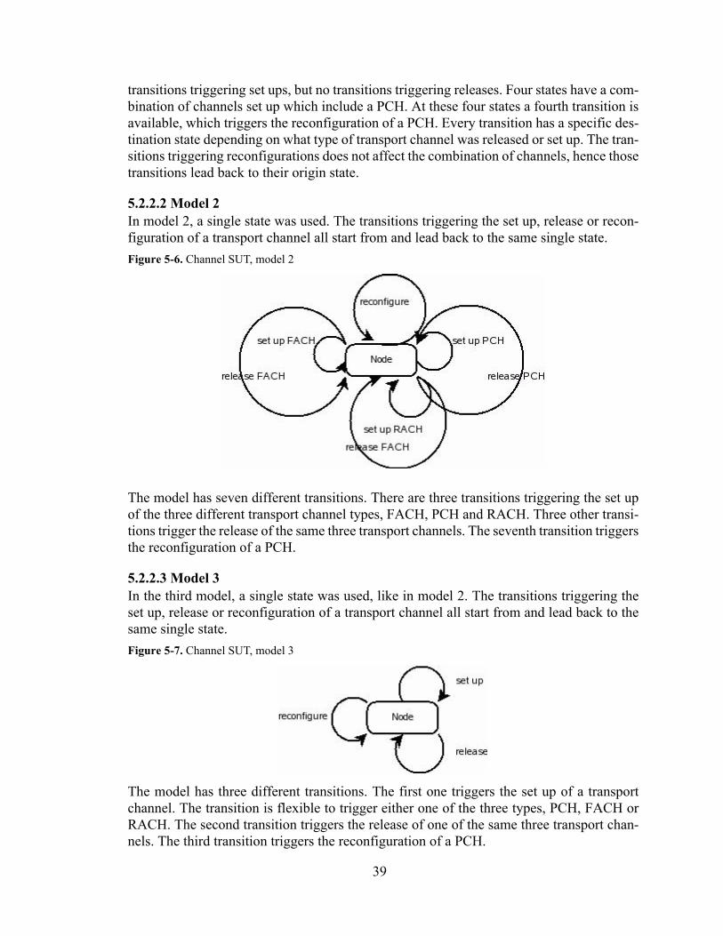
39

transitions triggering set ups, but no transitions triggering releases. Four states have a com-bination of channels set up which include a PCH. At these four states a fourth transition is available, which triggers the reconfiguration of a PCH. Every transition has a specific des-tination state depending on what type of transport channel was released or set up. The tran-sitions triggering reconfigurations does not affect the combination of channels, hence those transitions lead back to their origin state.

5.2.2.2 Model 2

Figure 5-6. Channel SUT, model 2

In model 2, a single state was used. The transitions triggering the set up, release or recon-figuration of a transport channel all start from and lead back to the same single state.

The model has seven different transitions. There are three transitions triggering the set up of the three different transport channel types, FACH, PCH and RACH. Three other transi-tions trigger the release of the same three transport channels. The seventh transition triggersthe reconfiguration of a PCH.

5.2.2.3 Model 3

Figure 5-7. Channel SUT, model 3

In the third model, a single state was used, like in model 2. The transitions triggering the set up, release or reconfiguration of a transport channel all start from and lead back to the same single state.

The model has three different transitions. The first one triggers the set up of a transport channel. The transition is flexible to trigger either one of the three types, PCH, FACH or RACH. The second transition triggers the release of one of the same three transport chan-nels. The third transition triggers the reconfiguration of a PCH.

40

5.2.3 QuickCheck implementationThe finite state machine models were converted to Erlang code according to QuickCheck’s eqc_fsm module policy. The purpose of this code was to use the eqc_fsm module and implement QuickCheck tests covering the functionality of the chosen SUT.

5.2.3.1 Model 1The eight states of the finite state machine model were represented in Erlang code as a single eqc_fsm callback function. This function is flexible to handle the behavior of the whole finite state machine. It has a state name containing three variables to represent the number of transport channels currently set up. The callback function has constraints on the three variables which determine what transitions are available from the current state. E.g. if all of the variables are zero, i.e. when no channels are set up, the constraints prevent any release transitions from being available in that state. Depending on the variables and their constraints, a list of available transitions from the current state is generated and returned to eqc_fsm from the callback function. The list of transitions includes information about the target state for each transition by indicating how the state name variables should be updated when a transition occurs. E.g. when a transition trigger the set up of a PCH, the variable corresponding to the number of set up PCHs is increased by one. This enables the traverse from one state to another by the use of one of the available transitions.An Erlang record is used to keep track of any set up PCH, RACH or FACHs. This record is updated when a transition occurs which affects the presence of these channels. The infor-mation in the record is used solely to clean up the SUT in between tests cases, returning it to its initial state containing no set up channels. This information is also available through the state name variables. However, the occurrence of an error in a transition could corrupt the information in the state name variables. Hence, an Erlang record is used to store the information.Every transition calls a function that invokes a module which creates an appropriate NBAP message and sends it to the SUT, in order to test its functionality. The NBAP messages are created and sent using the npap.ctcm module. For the messages sent to invoke a set up or release, the NBAP messages are created specifying the target type of transport channel (PCH, RACH or FACH) while the reconfiguration NBAP messages require additional specification of the power value of the channel. This value is generated randomly within an interval using a QuickCheck generator. After the messages are sent, the functions return the response message from the SUT, which can be analyzed by QuickCheck to determine if the SUT responds according to its specification. Also, the actual number of PCH, RACH and FACHs set up is checked using the mub_mo module. These values are compared to the state name variables, verifying that each request for a channel set up or release has been met. The analysis is done in QuickCheck’s postcondition callback function.

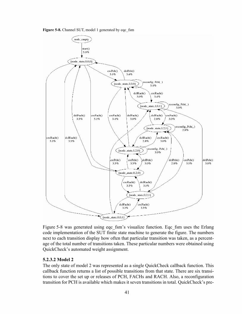
Figure 5-8. Channel SUT, model 1 generated by eqc_fsm

41

Figure 5-8 was generated using eqc_fsm’s visualize function. Eqc_fsm uses the Erlang code implementation of the SUT finite state machine to generate the figure. The numbers next to each transition display how often that particular transition was taken, as a percent-age of the total number of transitions taken. These particular numbers were obtained using QuickCheck’s automated weight assignment.

5.2.3.2 Model 2The only state of model 2 was represented as a single QuickCheck callback function. This callback function returns a list of possible transitions from that state. There are six transi-tions to cover the set up or releases of PCH, FACHs and RACH. Also, a reconfiguration transition for PCH is available which makes it seven transitions in total. QuickCheck’s pre-

42

condition function is used to determine what transitions are allowed in the current state, depending on which channels are set up. E.g. if no channels are set up, a transition trigger-ing the release of a channel will be excluded from the list of available transitions returned from the state callback function.The transitions invoke functions which use nbap.ctcm to construct and send NBAP mes-sages over iub to the SUT. Information about the target SUT and the type of transport chan-nel in question for the specific operation is specified in the function called by each transition. Also, the reconfiguration transition specifies the power value of the channel. This value is generated by a QuickCheck generator and will be included in the NBAP mes-sage created by the function corresponding to the reconfiguration transition.With every transition, an Erlang record is passed on to the next state. This record is updated after every transition with information about the number of set up channels. This informa-tion is used to verify the behavior of the SUT and to revert it back to its initial state in between test cases.

Figure 5-9. Channel SUT, model 2 generated by eqc_fsm.

The behavior of the SUT is verified by using mp_mub to read the number of set up channels and comparing those values to the values in the Erlang record. The NBAP response mes-sage sent back from the SUT is also analyzed to ensure correct behavior. The analysis and verification is done in the postcondition callback function.

Figure 5-9 was generated using eqc_fsm’s visualize function. Eqc_fsm uses the Erlang code implementation of the SUT finite state machine to generate the figure. The numbers next to each transition display how often that particular transition was taken, as a percent-age of the total number of transitions taken. These particular numbers were obtained using QuickCheck’s automated weight assignment.

5.2.3.3 Model 3The single state of model 3 was represented as a QuickCheck callback function, returning a list of available transitions from the state. Three different transitions are available: set up, release and reconfiguration. An Erlang record is updated with every transition. The record contains two lists. The first contains the names of the transport channel types which are set up and the second list contains the names of the channels which have not yet been set up. At the initial state, the second list contains the names of the three channel types PCH, FACH and RACH, and the first list is empty. A transition for the set up of a certain channel will transfer the name of that channel type from the not-set up list to the set up list. A release transition would transfer the name in the opposite direction, from the set up list to the not-set up list. The release and set up transitions require the name of the target channel type to be specified. A QuickCheck generator is used to randomly select one of the type names from one of the list in the record. A set up transition will choose one of the elements in the

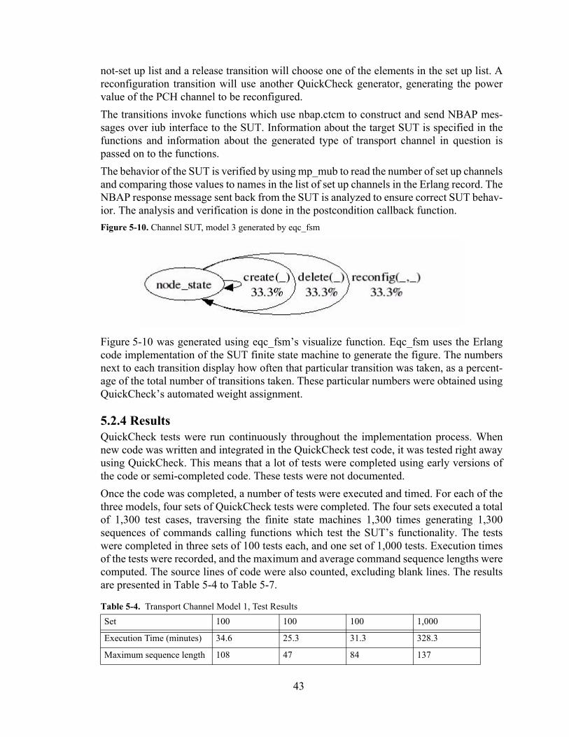
43

not-set up list and a release transition will choose one of the elements in the set up list. A reconfiguration transition will use another QuickCheck generator, generating the power value of the PCH channel to be reconfigured.The transitions invoke functions which use nbap.ctcm to construct and send NBAP mes-sages over iub interface to the SUT. Information about the target SUT is specified in the functions and information about the generated type of transport channel in question is passed on to the functions.

Figure 5-10. Channel SUT, model 3 generated by eqc_fsm

The behavior of the SUT is verified by using mp_mub to read the number of set up channels and comparing those values to names in the list of set up channels in the Erlang record. The NBAP response message sent back from the SUT is analyzed to ensure correct SUT behav-ior. The analysis and verification is done in the postcondition callback function.

Figure 5-10 was generated using eqc_fsm’s visualize function. Eqc_fsm uses the Erlang code implementation of the SUT finite state machine to generate the figure. The numbers next to each transition display how often that particular transition was taken, as a percent-age of the total number of transitions taken. These particular numbers were obtained using QuickCheck’s automated weight assignment.

5.2.4 ResultsQuickCheck tests were run continuously throughout the implementation process. When new code was written and integrated in the QuickCheck test code, it was tested right away using QuickCheck. This means that a lot of tests were completed using early versions of the code or semi-completed code. These tests were not documented.Once the code was completed, a number of tests were executed and timed. For each of the three models, four sets of QuickCheck tests were completed. The four sets executed a total of 1,300 test cases, traversing the finite state machines 1,300 times generating 1,300 sequences of commands calling functions which test the SUT’s functionality. The tests were completed in three sets of 100 tests each, and one set of 1,000 tests. Execution timesof the tests were recorded, and the maximum and average command sequence lengths were computed. The source lines of code were also counted, excluding blank lines. The results are presented in Table 5-4 to Table 5-7.

Table 5-4. Transport Channel Model 1, Test ResultsSet 100 100 100 1,000

Execution Time (minutes) 34.6 25.3 31.3 328.3

Maximum sequence length 108 47 84 137

44

5.3 Fictive SystemThis system is fictive. The characteristics included in the following description were chosen in order to theoretically construct a system which would be of interest to analyze in this thesis work, as a complement to the two SUT’s investigated in practice.

5.3.1 SUT DescriptionThe documentation describing this system provided information about the different natural states of the system. Every action or function that the system performs was described in the documentation along with information about the resulting state of the system.The system has interactions with other systems. However, these interactions are of the nature that they can be simulated. The simulations would work in such a way that the inter-actions can be performed without the occurance of an error in the other systems while still performing the interactions in an accurate way.The system has different functionalities. When triggered, some of the functionalities leave the system in an unaltered state, while others transfer the system into a new state where dif-

Average sequence length 16.4 11.6 14.5 15.3

SUT errors found 0 0 0 0

Table 5-5. Transport Channel Model 2, Test ResultsSet 100 100 100 1,000

Execution Time (minutes) 31.3 32.9 33.8 365.8

Maximum sequence length 109 76 76 106

Average sequence length 13.5 14.6 14.9 15.4

SUT errors found 0 0 0 0

Table 5-6. Transport Channel Model 3, Test ResultsSet 100 100 100 1,000

Execution Time (minutes) 30.5 27.5 33.5 336.9

Maximum sequence length 55 81 89 94

Average sequence length 13.47 12.4 15.3 15.4

SUT errors found 0 0 0 0

Table 5-7. Transport Channels QuickCheck Specification Source Lines of CodeModel 1 Model 2 Model 3

Comment 23 21 21

Code 187 222 122

Total 210 243 143

Table 5-4. Transport Channel Model 1, Test ResultsSet 100 100 100 1,000

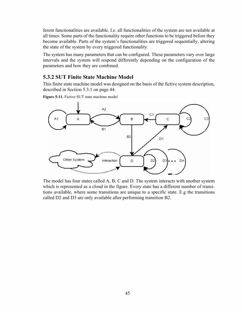
45

ferent functionalities are available. I.e. all functionalities of the system are not available at all times. Some parts of the functionality require other functions to be triggered before they become available. Parts of the system’s functionalities are triggered sequentially, altering the state of the system by every triggered functionality.The system has many parameters that can be configured. These parameters vary over large intervals and the system will respond differently depending on the configuration of the parameters and how they are combined.

5.3.2 SUT Finite State Machine Model

Figure 5-11. Fictive SUT state machine model

This finite state machine model was designed on the basis of the fictive system description, described in Section 5.3.1 on page 44.

The model has four states called A, B, C and D. The system interacts with another system which is represented as a cloud in the figure. Every state has a different number of transi-tions available, where some transitions are unique to a specific state. E.g the transitions called D2 and D3 are only available after performing transition B2.

46

47

6Analysis

6.1 EC Characteristics AnalysisThe first SUT that was modelled and tested using QuickCheck was a demarcated part of the NPR, which contained the functionality to set up and release subracks in the Node B. The SUT was modeled as two different state machines. The first state machine, model 1, consisted of two states, one state where no subracks are set up (empty_state) and another state where subracks are set up (rack_state). The second state machine, model 2, consisted of eight different states representing the number of subracks currently set up in the SUT. The same SUT can be modeled as different finite state machines depending on the user’s choice. QuickCheck could successfully test both of the models above. They could also be implemented according to eqc_fsm, using relatively few source lines of code. This SUT had very few interactions and dependencies with other systems and if the SUT was coded as a finite state machine using QuickCheck it had few natural states. The signals sent to the SUT requesting the set up or release of a subrack contained few parameters and there were few transitions between the states.

6.1.1 Few Interactions and DependenciesAs mentioned, the SUT had few interactions and dependencies with other systems. This facilitated the process of finding a finite state machine of the SUT, e.g. because the SUT was the only actor responsible for handling the subracks. The two models of the SUT were both affected in the same way by this characteristic. It enabled all the transitions in both of the models to be implemented in a straightforward way, without taking account for any actions played out by other systems. Once a finite state machine had been found, it could easily be transferred to code according to QuickCheck’s eqc_fsm module. This code could then be used to run QuickCheck tests of the SUT.

6.1.2 Few Natural StatesThis SUT had almost no natural states at all when it was to be modelled as a finite state machine using eqc_fsm in QuickCheck. Since the functionality of the SUT also was lim-ited, the few natural states that did exist did not have to consider and handle more than the two functionalities that the SUT had. The SUT could be modelled in different ways and all of these different finite state machines could be converted to code according to eqc_fsm’s guiding principles. This allows the QuickCheck user to choose which finite state machine he or she wants to implement. This enables the user to work with a model which suits his or her testing preferences, possibly making the work more efficient and fun.

48

6.1.3 Few ParametersThe signals sent to the SUT requesting the set up or release of a subrack contained only one parameter to be generated and handled by QuickCheck. It was the parameter which speci-fied the identification number for each subrack. This parameter could be generated and han-dled by QuickCheck’s eqc_fsm module without any difficulties. Having only one parameter did not affect any of the two models differently. They could both use similar gen-erators to generate the parameter that should be included in the signals sent to the SUT.

6.1.4 Few Transitions Between the StatesThis SUT was simple to model with eqc_fsm, since it only had two functionalities: set up and release subracks in the Node B. These were also the same transitions that could be made in the finite state machines, but sometimes they had conditions attached to them, e.g. a release of a specific subrack could not be done if the same subrack had not yet been set up in the Node B. The characteristic of having few transitions affected the two models of the SUT in the same way. They both had the same, few transitions to choose from in their states. Eqc_fsm has the capability to handle the implementation of these few transitions and their constraints without any problem.

6.2 Transport Channels Characteristics AnalysisThe second SUT that was modelled and tested using QuickCheck was a demarcated part of the MPSW, which contained the functionality to set up, reconfigure and release transport channels in the Node B. Three different finite state machine models of the SUT were designed. The first state mach-ine consisted of eight states, each representing a specific combination of transport channels set up in the SUT. The second and third state machine models each consisted of one state. In the first model, three or four transitions were available from each state depending on the combination of transport channels set up in the SUT. In the second model, seven transitions were available from its single state, compared to three transitions that were available in the third model.This SUT had very few interactions and dependencies with other systems and if the SUT was coded as a finite state machine using QuickCheck it had few natural states. The signals sent to the SUT requesting the set up, reconfigure or release of a transport channel con-tained few parameters and there were few transitions between the states.

6.2.1 Few Interactions and Dependencies One of the SUT’s characteristics was that it had few interactions and dependencies with other systems. This made it easier to construct an eqc_fsm finite state machine of the SUT, since no consideration had to be taken regarding the interference of other systems. In all of the three models, the SUT’s characteristic of having few interactions and dependencies affected the Erlang code in the same way. It enabled all of the functions invoked by a tran-sition to execute its testing code on the SUT in a straightforward manner, without taking account for the behavior and actions of other systems.

49

6.2.2 Few Natural States As mentioned, the SUT had few interactions and dependencies and also few transitions between its states. These characteristics combined with the characteristic of having few nat-ural states made the finite state machine model of the SUT finite, as the model did not branch off into an unlimited amount of related subsystems. Hence, the SUT could success-fully be modelled according to eqc_fsm and tested using QuickCheck. The idea was to design finite state machines with different characteristics in order to inves-tigate the applicability of eqc_fsm. In the first model, an attempt was made to design a finite state machine with as many states as possible derived from the few natural states available. The number of states was extended by using a unique state for each combination of trans-port channels in the SUT. Every state had to be implemented in Erlang code, and eqc_fsm provided the option to implement several states at once using a state combination with a state name variable. This state could then cover an arbitrary number of states defined by boundaries on the state name variable. Eqc_fsm is capable of conveniently handling a SUT finite state machine consisting of several states which origin from a SUT with few natural states.Since the SUT itself had few natural states, a more natural way to model the SUT, com-pared to the first model, was with a minimal finite state machine containing one single state. The second and the third finite state machines were both modelled in this way, using one state each. Eqc_fsm is capable of handling finite state machines with only one state, mod-elled from SUTs with few natural states.

6.2.3 Few Parameters Another characteristic of this SUT was that the signals sent to the SUT to test its function-ality had few parameters. The number of parameters in the signals sent to the SUT did not affect the applicability of eqc_fsm. QuickCheck has the potential to handle a large number of parameters. Altogether the three models used two parameters which were generated using QuickCheck generators.

6.2.4 Few Transitions Between the StatesThe last characteristic of the SUT was that it had quite few transitions between the states. This characteristic made eqc_fsm applicable as a testing tool of the SUT, because eqc_fsm can handle finite state machines containing any number of transitions between its states. All three models of the SUT had a different number of transitions. In the second and third models all transitions started and ended in the models’ single states, while the first model had different combinations of transitions for each of its eight states. Eqc_fsm is flexible to allow the user to define any number of transitions. These transitions can be defined to start from the same state or defined to start from different states, divided arbitrarily. Hence, eqc_fsm was capable of handling the different number of transitions found in all of the three finite state machines.

50

6.3 Test Results AnalysisAt the LTC, test commands are written one by one in Erlang modules. For example, one file at the LTC contained commands to test the set up, release and reconfiguration of trans-port channels in the LTC’s MPSW. This file contained test cases which all tested the set up, release or reconfigure of a transport channel in different ways, e.g using variations of the parameters included in the NBAP messages sent to the SUT by the commands. The SUTs tested in this thesis were less complex than the corresponding subsystem of the LTC’s MPSW. Hence, the commands to test the SUTs in this thesis were not as complex as the commands used at the LTC to test their MPSW, e.g. they did not include as many variations of the parameters in the NBAP messages. Nevertheless, the Erlang QuickCheck code was more than ten times shorter and had the capability to produce an infinite amount of unique commands. E.g. one QuickCheck test of the SUT executed more than a hundred times more commands than what was included in the LTC’s Erlang modules, while using test code which was ten times shorter than the LTC’s Erlang module.These numbers indicate that eqc_fsm can be used to generate a larger number of unique test commands using less source lines of code compared to writing test cases in a one to one fashion like the tests used at LTC.

6.4 Fictive SUT Characteristics Analysis

6.4.1 DocumentationThe documentation describing the system was already oriented towards describing the nat-ural states of the system. This facilitated the process of modelling a finite state machine of the system.

6.4.2 Interactions and DependenciesThe system had interactions and dependencies with other systems, but the behavior of the other systems could be simulated. This enabled all of the functionality of the system to be tested in a straightforward manner, with the interactions and dependencies developing as desired. Once the interactions and dependencies could be anticipated, the other systems did not have to be included in the finite state machine of the system. Only the system itself had to be included in the model. Once a finite state machine had been modeled, it could be trans-ferred to Erlang code according to eqc_fsm’s representation of finite state machines and tested using QuickCheck.

6.4.3 States and TransitionsThe finite state machine model of the system includes several different states with different transitions. Eqc_fsm’s representation of models in Erlang code provide a means to effi-ciently transfer a finite state machine model to code, while maintaining a natural structure of the state machine. Each representation of a state will be organized together with the rep-resentation of the transitions available from that state.

51

6.4.4 ParametersThe many parameters of the system range over large intervals and they can be configured in different combinations. The system will respond to different configurations in different ways. This allows for a huge amount of possible test cases of the system. QuickCheck can cover these test cases by randomly choosing a combination of the parameters from the dif-ferent intervals and use this random selection for a test case. This provides a way of cover-ing all of the combinations, when enough tests cases are executed, still using the same amount of code.

52

53

7Discussion

7.1 The SUTsThe two SUTs that were chosen to be modelled and tested using QuickCheck were suitable systems to use for answering the problem definition of this thesis. They were small, did not have that much functionality nor interaction and dependencies with other systems and they were not too complex to understand. The main reason for choosing systems with these char-acteristics was to facilitate the testing and modelling of these systems using QuickCheck. The idea was that these systems would assure that there were no obstacles in the way when doing so. Time could then be spend on evaluating eqc_fsm instead of learning, working and solving different issues that might arise with more complex systems. The systems were both successfully modelled according to eqc_fsm and tested using QuickCheck. This showed that QuickCheck’s eqc_fsm module was applicable as a testing tool for these two systems. However, the systems were too small to make use of eqc_fsm’s full capability. With larger and more complex systems one might come up with a different evaluation of eqc_fsm, since things could be found that where unintentionally overseen in this evaluation due to the limited size and complexity of the tested SUTs. Even though the systems were not that large and complex, it took time to learn how to send the signals and with what parameters, telling the SUT what action to perform. A lot of time was spent on getting this part to work. So if the chosen systems would have been larger than they were, the part with sending signals would probably have taken much longer, leaving less time for the evaluation of eqc_fsm.

7.2 The Work

7.2.1 Obtaining KnowledgeThere was a lot of new knowledge to be obtained when starting writing this master thesis at the LTC regarding the systems at LTC. For example, many unfamiliar commands had to be learnt to be able to use most of the systems and programs there. It was even difficult to find specific documents and information without knowing exactly where to look. This made the start of the thesis work feel a bit slow. Hence, it took some time to actually start working with it. This might be the case with most master theses though, since one often needs to know things surrounding the thesis to be able to start, work and finish it. One thing that took a very long time was to figure out how to send all the signals, from erlang to the Node B for example. Out of 19 days when working with the NPR and the sub-racks, only four days was spent on implementing the QuickCheck code, while the rest of the time was spent on getting the signals right. This felt a bit unbalanced, since learning

54

how to send and receive signals was not really a part of this thesis. Of course we expected to work with things around the actual task, but not this much. The other way around, work-ing 15 days with the QuickCheck implementation would have been more preferable.

7.2.2 Critical Revise of the Methods UsedAll of the material used in this thesis about QuickCheck has been written or at least partly written by the founders of QuickCheck, Hughes and Arts. Apart from teaching us the basics about QuickCheck in the three day QuickCheck course, John and Thomas also visited us after that. Then they e.g. answered any questions that might have arisen since last time, explained how the written QuickCheck code could be improved or come up with sugges-tions of how a problem could be solved using QuickCheck. One of the master theses in the chapter Previous Work, "Testing a radiotherapy support system with QuickCheck", was supervised by Thomas Arts. The authors of the other master thesis in the same chapter, "NBAP message construction using QuickCheck", attended the same QuickCheck course as we did and they were also visited by John and Thomas a couple of times during their thesis work. The fact that John and Thomas has been involved with everything we have read and learned concerning QuickCheck could make one wonder if the evaluation of QuickCheck’s eqc_fsm module has been made without their influences. From their point of view Quick-Check is an excellent testing tool that could and should be used by more companies. They believe that it would facilitate much for those who choose to use it, that using QuickCheck would save time and find errors that would not have been found prior to using QuickCheck. We have been aware of their opinions throughout the work of this thesis and do not think that we have been affected by their positive thinking about QuickCheck. However, we do think the best of QuickCheck, because of everything we have experienced when working with the tool over the last six months.

7.3 The Result We consider that the problem definition on the basis of the scope of this thesis has been answered. A number of SUT characteristics have been identified and isolated in order to analyze them and evaluate their impact on the applicability of eqc_fsm on the SUT.Perhaps more system characteristics could have been found if the systems modelled and tested using QuickCheck had been larger and more complex than the systems that were actually used.

7.4 What Could Have Been Done Better As mentioned earlier more time could have been spent on implementing code in Quick-Check and evaluating the eqc_fsm and the systems characteristics. Due to surrounding issues, e.g. the time it took to learn how to send and receive signals to the SUTs and due to the time limitation of this thesis work, this is not really anything we could have changed. Maybe we could have pushed to get some more help regarding the work which was not related to QuickCheck use.

55

We did not have much knowledge about the different technologies used in WCDMA, nei-ther did we have any experience working with Erlang or QuickCheck. But we never felt that our lack of experience in these areas prevented us from reaching the goals of this thesis.

7.5 Experiences It has been an instructive experience performing and writing the master thesis at the LTC. It has given an insight into a large international company and the sequence of work there.New knowledge about a never before used programming language, Erlang, has been obtained. We have also learnt how to handle and use the testing tool QuickCheck. Through this thesis we have strived to reach a goal, which e.g. has taught us to plan our time. Since this thesis has been a cooperation by two, it has improved our collaboration skills as well as the understanding for another person with other characteristics than one has. This is the longest time we have worked with a project as comprised as a master thesis.

To conclude, it has been both a fun and instructive experience to perform this master thesis at the LTC. We have gotten to know many competent, social and helpful people along theway. Much has been learned during these six months at the LTC and we have enjoyed working there.

56

57

8Conclusion

The systems investigated in this thesis were analyzed on the basis of their characteristics. A number of characteristics were identified, isolated and analyzed on how they affected the applicability of QuickCheck’s eqc_fsm module as a testing tool for the systems. These characteristics were that the system had:

• Few interactions and dependencies

• Few natural states

• Few parameters

• Few transitions between the states

The applicability of eqc_fsm as a testing tool for a software was not affected to a great degree by the characteristics investigated. Eqc_fsm was able to function well together with systems with these characteristics. Eqc_fsm was flexible to handle systems with different characteristics. For example, one characteristic was that a system had few natural states. This characteristic is not a preferred characteristic of a system which should be tested using eqc_fsm. Still, this characteristic resulted in certain functionalities in eqc_fsm becoming superfluous, rather than preventing eqc_fsm from being capable to apply as a testing tool for that software.Two subsystems of the LTC’s Node B software were investigated and tested using Quick-Check’s eqc_fsm module. Eqc_fsm was found to be applicable as a testing tool for these subsystems. This indicates that QuickCheck’s eqc_fsm module could be a suitable tool for testing the Node B software.

58

59

9Future work

To further analyze QuickCheck, eqc_fsm and its applicability as a testing tool for the soft-ware at the LTC, one could continue and extend the work of this thesis.The scope could be widened to include more and larger systems. These systems could be investigated in order to see if it is possible to find characteristics which were not found in the systems investigated in this thesis. These characteristics could then be analyzed to determine how they affect the applicability of eqc_fsm.Another possible extension of the work in this thesis could be to investigate one of the test suites at the LTC. There are many different test suites and they all include a number of test cases which test different systems of the LTC’s software. It would be interesting to try to cover every test case in the suite with a single QuickCheck property, using eqc_fsm. This would give more relevant results on the benefits of using QuickCheck in terms of source code length, test execution time and test coverage.This idea could also be extended further by investigating if the test cases of several different test suites could be covered by a single QuickCheck property. Perhaps all the test suites at the LTC could be replaced by a single QuickCheck property!?

60

61

10References

10.1 Literature

10.1.1 Books• Holma, H & Toskala, A. (eds.). WCDMA for UMTS. John Wiley & Sons, Ltd (2001).

ISBN 0-471-48687-6.

• Dahlman, E., Parkvall, S. Sköld, J. & Beming, P. 3G Evolution HSPA and LTE for Mobile Broadband. Elsevier Science & Technology (2008). ISBN 0-123-74538-1.

• Cesarini, F. & Thompson, S. Erlang Programming. O’Reilly Media (2009). ISBN 0-596-51818-9.

10.1.2 Articles • Hughes, J. QuickCheck Testing for Fun and Profit. pp 1-33 in Hanus, M., Practical

Aspects of Declarative Languages. Springer-Verlag Berlin Heidelberg (2007). ISBN 3-540-69608-3.

• Granberg, A. & Jernberg, D. NBAP message constructing using QuickCheck. Master’s thesis, Department of Computer Science, Linköping University (2007). ISRN LITH-IDA-EX--07/033--SE.

• Yamashita, A. & Bergqvist, A. Testing a radiotherapy support system with Quick-Check. Master’s thesis, Report no. 2007:62, Department of Applied Information Tech-nology, IT University of Göteborg (2007). ISSN 1651-4769.

• Ericsson Radio Systems AB. White Paper - Basic Concepts of WCDMA Radio Access Network. Ericsson Radio Systems AB (2001). AE/LZT 123 6982.

10.1.3 Technical Specifications • 3GPP, TS 25.211 V8.5.0 - Physical channels and mapping of transport channels onto

physical channels (Release 8) (2009-09)

• 3GPP, TS 25.433 version 7.14.0 Release 7 - UTRAN Iub interface Node B Application Part (NBAP) signalling, ETSI TS 125 433 V7.14.0 (2009-10)

• QuviQ - QuickCheck for Erlang Users, 2009

62

10.1.4 Internet Sources• Claessen, K. & Hughes, J. (2000). QuickCheck: A Lightweight Tool for Random Test-

ing of Haskell Programs, http://types.bu.edu/reading-group/documents/QuickCheck-slides.pdf, 2010-04-01

• History of Erlang, http://erlang.org/course/history.html, 2010-04-01

• Common Test Basics, http://www.erlang.org/doc/apps/common_test/basics_chapter.html, 2010-04-01

• About us, http://www.quviq.com, 2010-04-01

• InfoQ, http://www.infoq.com/interviews/Erlang-Haskell-John-Hughes, 2010-04-01

• Claessen, Koen, Palka, Michal, Smallbone, Nicholas, Hughes, John, Svensson, Hans, Arts, Thomas and Wiger, Ulf (2009), Finding Race Conditions in Erlang with Quick-Check and PULSE, http://www.protest-project.eu/upload/paper/icfp070-claessen.pdf, 2010-04-01.

10.1.5 LTC’s Classified Documents• Equipment Control Subsystem Overview, LTC classified document.

• Node B workshop, LTC classified document.

• The ct_mo application - Mub access, LTC classified document.

• The Bp application, LTC classified document.

• The Iub application, LTC classified document.

10.1.6 Software files• QuickCheck function index, which is a file included in the QuickCheck distribution.

63

11Appendix

11.1 Erlang Code

11.1.1 EC SUT Model 1 QuickCheck Eqc_fsm Implementation-module(fsrm1).

-include_lib("eqc/include/eqc.hrl").-include_lib("eqc/include/eqc_fsm.hrl").-include("/vobs/rbs/sw/rbsswiov_target_1/test_root/lib/bp/include/bp.hrl").

-compile(export_all).

-record(sdata,{racksInfo = [{rbs,[]}] }).

%%%%% START OF HELP-FKN %%%%%%%%%%%%%%%%%%%%%%%%%%%%%%%%%%%%%%%%5 getRackValue(S,RackType) -> proplists:get_value(RackType,S#sdata.racksInfo,finnnsEjtypen).

totalRacks(S) -> lists:sum([ length(Value) || {_,Value} <- S#sdata.racksInfo ]).

setRackValue(S,RackType,X) -> S#sdata{racksInfo = ([{RackType,X}] ++ (proplists:delete(RackType,S#sdata.racksInfo))) }.

addRack(S,RackType,Id) -> setRackValue(S,RackType, lists:usort(getRackValue(S,RackType)++[Id]) ) .

deleteRack(S,RackType,Id) -> setRackValue(S,RackType, (getRackValue(S,RackType)--[Id] )).

get_ose_pid(ProcessName) -> element(2,bp:hunt_ose_pid(mp_bp,ProcessName)).

return_Xmos(MoTypeString) -> length(element(2,mub_mo:getChildren(mp_mub,"ManagedElement=1,Equipment=1",[{type,MoTypeString}]))).

moString(rbs,Id) -> "ManagedElement=1,Equipment=1,RbsSubrack="++integer_to_list(Id). %%%%%%% SLUT PA HJELP FKN %%%%%%%%%%%%%%%%%%%%%%%%%%%%%%%%%%%%%%%%%%%%%

delete_rack(RackType,Id) -> MoString = moString(RackType,Id), Result = mub_mo:delete(mp_mub,MoString,[]), Result.

create_rack(RackType,Id) -> MoString = moString(RackType,Id), Result = mub_mo:create(mp_mub,MoString,[]), Result.

%%%%%%%%%%%%%% Generators %%%%%%%%%%%%%%%%%%%%%%%%%%%%%%%%%%%%%%%%%%%%%%%%%%%%%%

rbsNumberGen() -> choose(11,36).

rackTypeGen() -> elements([rbs]).

idGen(S,RackType) -> elements(getRackValue(S,RackType)).

existingTypeGen(S) -> elements( [ RackType || {RackType, IdList} <- S#sdata.racksInfo,

IdList /= [] ] ).

delete_rackArgGen(S) -> ?LET( RackType, existingTypeGen(S),

[RackType,idGen(S,RackType)] ).

%% Definition of the states. Each state is represented by a function, %% listing the transitions from that state, together with generators %% for the calls to make each transition.empty_state(_S) -> [ %% {target_state,{call,?MODULE,target_function,[]}} {rack_state, {call,?MODULE,create_rack,[rackTypeGen(),rbsNumberGen()]}} ].

rack_state(S) -> [ {rack_state,{call,?MODULE,delete_rack, delete_rackArgGen(S)}}, %% l‰gg till h‰r "Om det ‰r sista racket hoppa t empty_r {empty_state,{call,?MODULE,delete_rack,delete_rackArgGen(S)}}, {rack_state,{call,?MODULE,create_rack, [rackTypeGen(),rbsNumberGen()]}} %% l'‰gg till om ‰r sista rack create hoppa fullState

64

].

%% Identify the initial stateinitial_state() -> empty_state.

%% Initialize the state datainitial_state_data() -> #sdata{ }.

%% Next state transformation for state data.%% S is the current state, From and To are srack_statate namesnext_state_data(empty_state,rack_state,S,_V,{call,_,create_rack,[RackType, Id]}) -> addRack(S,RackType,Id);

next_state_data(rack_state,_to,S,_V,{call,_,delete_rack,[RackType, Id]}) -> %%Om sista rack empty_state annars rack_state deleteRack(S,RackType,Id);

next_state_data(rack_state,rack_state,S,_V,{call,_,create_rack,[RackType,Id]}) -> case totalRacks(S) == 7 of

true -> S;false -> addRack(S,RackType,Id)

end.

precondition(rack_state,empty_state,S,{call,_,delete_rack,[RackType,Id]}) -> totalRacks(S)==1 andalso lists:member(Id, getRackValue(S,RackType) );

precondition(rack_state,rack_state,S,{call,_,delete_rack,[RackType,Id]}) -> totalRacks(S)>1 andalso lists:member(Id, getRackValue(S,RackType) );

precondition(_From,_To,_S,{call,_,_,_}) -> true.

%% Postcondition, checked after command has been evaluated%% OBS: S is the state before next_state_data(From,To,S,_,<command>) postcondition(_,_,S,{call,_,create_rack,[RackType,Id]}, Res) -> ExpectedOK = totalRacks(S)<7 andalso not lists:member(Id, getRackValue(S,RackType)) , case Res of {error, _} -> not ExpectedOK; {ok,_} -> true %%( return_Xmos("RbsSubrack")==getRackValue(S,rbs) ) end;

postcondition(_,_,_S,{call,_,delete_rack,[_RackType,_Id]},Res) -> case Res of {error, _} -> false; ok -> true %%( return_Xmos("RbsSubrack")==getRackValue(S,rbs) ) end;

postcondition(_,_,_,_,_) -> true.

clearNode({_, S}) -> [ delete_rack(RackType, Id) || {RackType,Ids} <- S#sdata.racksInfo,

Id <- Ids ].

prop_machine() -> ?FORALL(Cmds, commands(?MODULE),

begin{H,S,Res} = run_commands(?MODULE,Cmds),clearNode(S),?WHENFAIL( io:format("History: ~p\nState: ~p\nRes: ~p\n",[H,S,Res]), measure(num_commands, length(Cmds),

%% collect(length(Cmds),%% aggregate(zip(state_names(H),%% command_names(Cmds)),

Res == ok) ) end).

test(Num) -> quickcheck(numtests(Num, prop_machine())).

timetest(Num) -> {MicroSeconds,Result} = timer:tc(?MODULE,test,[Num]), io:format("Seconds: ~p~n",[(MicroSeconds/1000000)]), io:format("Minutes: ~p~n",[(MicroSeconds/1000000/60)]), Result.

%% Weight for transition (this callback is optional).%% Specify how often each transition should be chosen

%% Weights generated automatically by: eqc_fsm:automate_weights(fsrm1).weight(empty_state,rack_state,{call,fsrm1,create_rack,[_,_]}) -> 1;weight(rack_state,empty_state,{call,fsrm1,delete_rack,_}) -> 1;weight(rack_state,rack_state,{call,fsrm1,create_rack,[_,_]}) -> 1;weight(rack_state,rack_state,{call,fsrm1,delete_rack,_}) -> 1.

11.1.2 EC SUT Model 2 QuickCheck Eqc_fsm Implementation-module(fsrm2).

-include_lib("eqc/include/eqc.hrl").-include_lib("eqc/include/eqc_fsm.hrl").-include("/vobs/rbs/sw/rbsswiov_target_1/test_root/lib/bp/include/bp.hrl").

-compile(export_all).

65

-record(sdata,{racksInfo = [{rbs,[]}] }). %% {rbs,5} ...

getRackValue(S,RackType) -> proplists:get_value(RackType,S#sdata.racksInfo,finnnsEjtypen).

totalRacks(S) -> length(takenIds(S)).

takenIds(S) -> lists:append([ Ids || {_,Ids} <- S#sdata.racksInfo ]).

setRackValue(S,RackType,X) -> S#sdata{racksInfo = ([{RackType,X}] ++ (proplists:delete(RackType,S#sdata.racksInfo))) }.

addRack(S,RackType,Id) -> setRackValue(S,RackType, lists:usort(getRackValue(S,RackType)++[Id]) ) .

deleteRack(S,RackType,Id) -> setRackValue(S,RackType, (getRackValue(S,RackType)--[Id] )).

get_ose_pid(ProcessName) -> element(2,bp:hunt_ose_pid(mp_bp,ProcessName)).

return_Xmos(MoTypeString) -> length(element(2,mub_mo:getChildren(mp_mub,"ManagedElement=1,Equipment=1",[{type,MoTypeString}]))).

moString(rbs,Id) -> "ManagedElement=1,Equipment=1,RbsSubrack="++integer_to_list(Id).

%%%%%%%%%%% Test funktions %%%%%%%%%%%%%%%%%%%%%%%%%%%%%%%%%%%

delete_rack(RackType,Id) -> MoString = moString(RackType,Id), Result = mub_mo:delete(mp_mub,MoString,[]), Result.

create_rack(RackType,Id) -> MoString = moString(RackType,Id), Result = mub_mo:create(mp_mub,MoString,[]), Result.

%% Generators %%%%%%%%%%%%%%%%%%%%%%%%%%%%%%%%%%%%%%%%%%%%%%%%%%%%%%

rbsNumberGen() -> choose(11,36).

rackTypeGen() -> elements([rbs]).

idGen(S,RackType) -> elements(getRackValue(S,RackType)).

existingTypeGen(S) -> elements( [ RackType || {RackType, IdList} <- S#sdata.racksInfo,

IdList /= [] ] ).

delete_rackArgGen(S) -> ?LET( RackType, existingTypeGen(S),

[RackType,idGen(S,RackType)] ).

freshIdGen(S) -> ?SUCHTHAT(Id, rbsNumberGen(), not lists:member(Id, takenIds(S))).

%% Definition of the states. Each state is represented by a function, %% listing the transitions from that state, together with generators %% for the calls to make each transition.rack_state(N, S) -> [ {{rack_state, N + 1}, {call, ?MODULE, create_rack, [rackTypeGen(), freshIdGen(S)]}}

|| true <- [N < 7] ] ++ [ {{rack_state, N}, {call, ?MODULE, create_rack, [rackTypeGen(), freshIdGen(S)]}}

|| true <- [N == 7] ] ++ [ {{rack_state, N}, {call, ?MODULE, create_rack, delete_rackArgGen(S)}} || true <- [N > 0 andalso N < 7] ] ++ [ {{rack_state, N - 1}, {call, ?MODULE, delete_rack, delete_rackArgGen(S)}} || true <- [N > 0] ].

%% Identify the initial stateinitial_state() -> {rack_state, 0}.

%% Initialize the state datainitial_state_data() -> #sdata{ }.

%% Next state transformation for state data.%% S is the current state, From and To are srack_statate namesnext_state_data({rack_state, 7}, {rack_state, 7}, S, _V, {call,_,create_rack,_}) -> S;

next_state_data(_From,_To,S,_V,{call,_,create_rack,[RackType, Id]}) -> addRack(S,RackType,Id);

next_state_data(_From,_To,S,_V,{call,_,delete_rack,[RackType, Id]}) -> deleteRack(S,RackType,Id).

%% Precondition (for sdata).%% Precondition is checked before command is added to the command sequenceprecondition(_From,_To,S,{call,_,delete_rack,[RackType, Id]}) -> lists:member(Id, getRackValue(S, RackType));

precondition({rack_state, N},{rack_state, N},S,{call,_,create_rack,[_RackType, Id]}) -> lists:member(Id, takenIds(S));

precondition({rack_state, N},{rack_state, M},S,{call,_,create_rack,[_RackType, Id]}) -> M == N + 1 andalso not lists:member(Id, takenIds(S));

66

precondition(_From,_To,_S,{call,_,_,_}) -> true.

%% Postcondition, checked after command has been evaluated%% OBS: S is the state before next_state_data(From,To,S,_,<command>) postcondition(_,_,_S,{call,_,delete_rack,_}, Res) -> Res == ok;postcondition(_,_,S,{call,_,create_rack,[_, Id]}, Res) -> ExpectOk = totalRacks(S) < 7 andalso not lists:member(Id, takenIds(S)), case Res of

{ok, _Trams} -> ExpectOk;{error, _} -> not ExpectOk

end.

clearNode({_, S}) -> [ delete_rack(RackType, Id) || {RackType,Ids} <- S#sdata.racksInfo,

Id <- Ids ].

prop_machine() -> ?FORALL(Cmds, commands(?MODULE),

begin{H,S,Res} = run_commands(?MODULE,Cmds),clearNode(S),?WHENFAIL( io:format("History: ~p\nState: ~p\nRes: ~p\n",[H,S,Res]), measure(num_commands, length(Cmds),

%% collect(length(Cmds),%% aggregate(zip(state_names(H),command_names(Cmds)), Res == ok)) %% ))

end).

test(Num) -> quickcheck(numtests(Num, prop_machine())).

timetest(Num) -> {MicroSeconds,Result} = timer:tc(?MODULE,test,[Num]), io:format("Seconds: ~p~n",[(MicroSeconds/1000000)]), io:format("Minutes: ~p~n",[(MicroSeconds/1000000/60)]), Result.

%% Weights generated automatically by: eqc_fsm:automate_weights(fsrm2).weight({rack_state,0},{rack_state,1},{call,fsrm2,create_rack,[_,_]}) -> 1;weight({rack_state,1},{rack_state,0},{call,fsrm2,delete_rack,_}) -> 1;weight({rack_state,1},{rack_state,1},{call,fsrm2,create_rack,_}) -> 1;weight({rack_state,1},{rack_state,2},{call,fsrm2,create_rack,[_,_]}) -> 2;weight({rack_state,2},{rack_state,1},{call,fsrm2,delete_rack,_}) -> 1;weight({rack_state,2},{rack_state,2},{call,fsrm2,create_rack,_}) -> 1;weight({rack_state,2},{rack_state,3},{call,fsrm2,create_rack,[_,_]}) -> 2;weight({rack_state,3},{rack_state,2},{call,fsrm2,delete_rack,_}) -> 2;weight({rack_state,3},{rack_state,3},{call,fsrm2,create_rack,_}) -> 2;weight({rack_state,3},{rack_state,4},{call,fsrm2,create_rack,[_,_]}) -> 5;weight({rack_state,4},{rack_state,3},{call,fsrm2,delete_rack,_}) -> 1;weight({rack_state,4},{rack_state,4},{call,fsrm2,create_rack,_}) -> 1;weight({rack_state,4},{rack_state,5},{call,fsrm2,create_rack,[_,_]}) -> 1;weight({rack_state,5},{rack_state,4},{call,fsrm2,delete_rack,_}) -> 1;weight({rack_state,5},{rack_state,5},{call,fsrm2,create_rack,_}) -> 1;weight({rack_state,5},{rack_state,6},{call,fsrm2,create_rack,[_,_]}) -> 2;weight({rack_state,6},{rack_state,5},{call,fsrm2,delete_rack,_}) -> 1;weight({rack_state,6},{rack_state,6},{call,fsrm2,create_rack,_}) -> 1;weight({rack_state,6},{rack_state,7},{call,fsrm2,create_rack,[_,_]}) -> 1;weight({rack_state,7},{rack_state,6},{call,fsrm2,delete_rack,_}) -> 1;weight({rack_state,7},{rack_state,7},{call,fsrm2,create_rack,[_,_]}) -> 1.

11.1.3 Transport Channel SUT Model 1 QuickCheck Eqc_fsm Implementation-module(fchm1).

-include_lib("eqc/include/eqc.hrl").-include_lib("eqc/include/eqc_fsm.hrl").

-compile(export_all).

-record(sdata,{antal_pch, antal_fach, antal_rach}).

%%%%%%%%%%%%%%%%%%%%%%%%%%% create och delete PCH %%%%%%%%%%%%%%%%%%%%%%crePch() -> [PhIdPch|_] = nbap.cch:getCommonPhysicalChannelIDs('Stand-alone SRB for PCCH on S-CCPCH'), aal2_server:start(), Resp = kanalSig:create_pch(), Sugr = hamtaSug( Resp ), aal2_server:connect(101,PhIdPch,Sugr), timer:sleep(500), Resp. delPch() -> [PhIdPch|_] = nbap.cch:getCommonPhysicalChannelIDs('Stand-alone SRB for PCCH on S-CCPCH'), Resp = kanalSig:delete_pch(), aal2_server:release(mp_iub,101,PhIdPch), timer:sleep(500), Resp.

%%%%%%%%%%%%%%%%%%%%%%%%%%% create och delete FACH %%%%%%%%%%%%%%%%%%%%%%%%%%%%%%%%%%%55

creFach() -> [PhIdFach|_] = nbap.cch:getCommonPhysicalChannelIDs('Interactive 32 kbps PS RB + SRBs for BCCH, CCCH, and DCCH on S-CCPCH'), aal2_server:start(), Resp = kanalSig:create_fach(), Sugr = hamtaSug( Resp ), aal2_server:connect(101,PhIdFach,Sugr), timer:sleep(500),

67

Resp. delFach() -> [PhIdFach|_] = nbap.cch:getCommonPhysicalChannelIDs('Interactive 32 kbps PS RB + SRBs for BCCH, CCCH, and DCCH on S-CCPCH'), Resp = kanalSig:delete_fach(), aal2_server:release(mp_iub,101,PhIdFach), timer:sleep(500), Resp.

%%%%%%%%%%%%%%%%%%%%%%%%%%%% create och delete RACH %%%%%%%%%%%%%%%%%%%%%%%%%%%%%%%%%%

creRach() -> [PhIdRach|_] = nbap.cch:getCommonPhysicalChannelIDs('Interactive 16 kbps PS RB + SRBs for CCCH, and DCCH on PRACH(20 ms TTI)'), aal2_server:start(), Resp = kanalSig:create_rach(), Sugr = hamtaSug( Resp ), aal2_server:connect(101,PhIdRach,Sugr), timer:sleep(500), Resp. delRach() -> [PhIdRach|_] = nbap.cch:getCommonPhysicalChannelIDs('Interactive 16 kbps PS RB + SRBs for CCCH, and DCCH on PRACH(20 ms TTI)'), Resp = kanalSig:delete_rach(), aal2_server:release(mp_iub,101,PhIdRach), timer:sleep(500), Resp.

%%%%%%%%%%%%%%%%%%%%%%%%%%%%%% Sugr hj‰lp %%%%%%%%%%%%%%%%%%%%%%%%%%%%%%%

hamtaSug(Resp) -> nbap.ctcm:getSugrsToConnect(halvaSvar(Resp)).

halvaSvar(Resp) -> lists:nth(2,tuple_to_list(Resp)).

%%%%%%%%%%%%%%%%%%%%%%%%%%%% Generatorer %%%%%%%%%%%%%%%%%%%%%%%%%%%%%%%%%%%%%%%

recPower() -> choose(75,120).

%%%%%%%%%%%%%%%%%%%%%%%%%% reconfigure %%%%%%%%%%%%%%%%%%%%%%%%%%%%%%%%%%%%

reconfig_Pch(Power) -> kanalSig:reconfig_Pch(Power). reconfig_Fach(Power) -> kanalSig:reconfig_Fach(Power).

reconfig_Rach(Power) -> kanalSig:reconfig_Rach(Power).

%%%%%%%%%%%%%%%%%%%%%%%%%%% start, ok, setup_cell %%%%%%%%%%%%%%%%%%%%%%%%%%

start() -> timer:sleep(10), ok.

setup_cell() -> util_debug:prepare(), util_common:cellSetup(mp_iub,-500,[601]).

nrOfMosOnNode(TypeString) -> case nrOfMosOnNodeHelp(TypeString) of

{error,_} -> 0;{ok,X} -> length(X)

end.

nrOfMosOnNodeHelp(TypeString) -> case TypeString of

"Pch" ->

mub_mo:getChildren(mp_mub,"ManagedElement=1,NodeBFunction=1,Sector=1,Carrier=1,Sccpch="++integer_to_list(20),[{type,TypeString}]); "Fach" ->

mub_mo:getChildren(mp_mub,"ManagedElement=1,NodeBFunction=1,Sector=1,Carrier=1,Sccpch="++integer_to_list(30),[{type,TypeString}]); "Rach" -> mub_mo:getChildren(mp_mub,"ManagedElement=1,NodeBFunction=1,Sector=1,Carrier=1,Prach="++integer_to_list(1),[{type,TypeString}])

end.

return_Xmos(Nr,MoTypeString) -> mub_mo:getChildren(mp_mub,"ManagedElement=1,NodeBFunction=1,Sector=1,Carrier=1,Sccpch="++integer_to_list(Nr),[{type,MoTypeString}]).

moString(rbs,Id) -> "ManagedElement=1,Equipment=1,RbsSubrack="++integer_to_list(Id).

nodCheck(Pch,Fach,Rach) -> PNod = nrOfMosOnNode("Pch"), FNod = nrOfMosOnNode("Fach"), RNod = nrOfMosOnNode("Rach"),

Pch == PNod andalsoFach == FNod andalsoRach == RNod.

resCheck(Res) ->case Res of ok -> true; {successfulOutcome,_} -> true; {unsuccessfulOutcome,_} -> false

end.

%% Definition of the states. Each state is represented by a function, %% listing the transitions from that state, together with generators %% for the calls to make each transition.node_empty(_S) ->

68

[ %% {targt_state,{call,?MODULE,target_function,[]}} { {node_state,0,0,0}, {call,?MODULE,start,[]}} ].

node_state(Pch,Fach,Rach,_S) -> [ {{node_state,Pch+1,Fach,Rach}, {call,?MODULE,crePch,[]} }

|| true <- [Pch < 1] ] ++ [ {{node_state,Pch,Fach+2,Rach}, {call,?MODULE,creFach,[]} }

|| true <- [Fach < 2] ] ++ [ {{node_state,Pch,Fach,Rach+1}, {call,?MODULE,creRach,[]} }

|| true <- [Rach < 1] ] ++ [ {{node_state,Pch-1,Fach,Rach}, {call,?MODULE,delPch,[]} }

|| true <- [Pch > 0] ] ++ [ {{node_state,Pch,Fach-2,Rach}, {call,?MODULE,delFach,[]} }

|| true <- [Fach > 0] ] ++ [ {{node_state,Pch,Fach,Rach-1}, {call,?MODULE,delRach,[]} }

|| true <- [Rach > 0] ] ++ [ {{node_state,Pch,Fach,Rach}, {call,?MODULE,reconfig_Pch,[recPower()]} }

|| true <- [Pch > 0] ].

%% ++%% [ {{node_state,Pch,Fach,Rach}, {call,?MODULE,reconfig_Fach,[recPower()]} }%% || true <- [Fach > 0] ] ++ %% Denna reconfig verkar inte funka p Fach, s ‰r som en Pch...%% [ {{node_state,Pch,Fach,Rach}, {call,?MODULE,reconfig_Rach,[recPower()]} }%% || true <- [Rach > 0] ]. %% Denna reconfig verkar inte funka p Fach, s ‰r som en Pch...

%% Identify the initial stateinitial_state() -> node_empty.

%% Initialize the state datainitial_state_data() -> #sdata{}.

%% Next state transformation for state data.timer:sleep(15000),%% S is the current state, From and To are state namesnext_state_data(node_empty,_To,S,_V,{call,_,start,_}) -> S#sdata{antal_pch = 0, antal_fach = 0, antal_rach = 0};

next_state_data(_From,_To,S,_V,{call,_,crePch,_}) -> S#sdata{antal_pch = (S#sdata.antal_pch + 1)};

next_state_data(_From,_To,S,_V,{call,_,creRach,_}) -> S#sdata{antal_rach = (S#sdata.antal_rach + 1)};

next_state_data(_From,_To,S,_V,{call,_,creFach,_}) -> S#sdata{antal_fach = (S#sdata.antal_fach + 2)};

next_state_data(_From,_To,S,_V,{call,_,delPch,_}) -> S#sdata{antal_pch = (S#sdata.antal_pch - 1)};

next_state_data(_From,_To,S,_V,{call,_,delRach,_}) -> S#sdata{antal_rach = (S#sdata.antal_rach - 1)};

next_state_data(_From,_To,S,_V,{call,_,delFach,_}) -> S#sdata{antal_fach = (S#sdata.antal_fach - 2)};

next_state_data(_From,_To,S,_V,{call,_,reconfig_Pch,_}) -> S;

next_state_data(_From,_To,S,_V,{call,_,reconfig_Fach,_}) -> S;

next_state_data(_From,_To,S,_V,{call,_,reconfig_Rach,_}) -> S;

next_state_data(_From,_To,S,_V,{call,_,_,_}) -> S.

%% Precondition (for state data).%% Precondition is checked before command is added to the command sequence%% precondition(node_state,{node_state,0,0,0},_S,{call,_,_,_}) ->%% true.

%%%%%%%%%%%%%%%%%%%% Preconditions %%%%%%%%%%%%%%%%%%%%%%%%%%%%%%

precondition(_From,_To,_S,{call,_,_,_}) -> true.

%%%%%%%%%%%%%%%%%%%% Postconditions %%%%%%%%%%%%%%%%%%%%%%%%%%%5

postcondition(_From,{node_state,Pch,Fach,Rach},_S,{call,_,_,_},Res) -> nodCheck(Pch,Fach,Rach) andalso resCheck(Res);

postcondition(_From,_To,_S,{call,_,_,_},_Res) -> true. clear_node({_,S}) ->case S of {sdata,undefined,undefined,undefined} -> ok; {sdata,_,_,_} ->

clearPch(S#sdata.antal_pch),clearRach(S#sdata.antal_rach),clearFach(S#sdata.antal_fach)

end.

clearPch(0) -> ok;clearPch(AntalPch) -> delPch(),

clearPch(AntalPch - 1).

clearFach(0) -> ok;clearFach(AntalFach) -> delFach(),

clearFach(AntalFach - 2).

clearRach(0) -> ok;clearRach(AntalRach) -> delRach(),

clearRach(AntalRach - 1).

69

prop_modell() -> ?FORALL(Cmds,commands(?MODULE),

begin{H,S,Res} = run_commands(?MODULE,Cmds),clear_node(S),?WHENFAIL( io:format("History: ~p\nState: ~p\nRes: ~p\n",[H,S,Res]), measure(num_commands, length(Cmds), Res == ok ) )

end).

test(N) -> eqc:quickcheck(numtests(N,prop_modell())).

timetest(Num) -> {MicroSeconds,Result} = timer:tc(?MODULE,test,[Num]), io:format("Seconds: ~p~n",[(MicroSeconds/1000000)]), io:format("Minutes: ~p~n",[(MicroSeconds/1000000/60)]), Result.

%% Weight for transition (this callback is optional).%% Specify how often each transition should be chosen

%% Weights generated automatically by: eqc_fsm:automate_weights(fsrm2).

11.1.4 Transport Channel SUT Model 2 QuickCheck Eqc_fsm Implementation-module(fchm2).

-include_lib("eqc/include/eqc.hrl").-include_lib("eqc/include/eqc_fsm.hrl").

-compile(export_all).

-record(sdata,{antal_pch = 0, antal_fach = 0, antal_rach = 0}).

%%%%%%%%%%%%%%%%%%%%%%%%%%% create och delete PCH %%%%%%%%%%%%%%%%%%%%%%crePch() -> [PhIdPch|_] = nbap.cch:getCommonPhysicalChannelIDs('Stand-alone SRB for PCCH on S-CCPCH'), aal2_server:start(), Resp = kanalSig:create_pch(), Sugr = hamtaSug( Resp ), aal2_server:connect(101,PhIdPch,Sugr), timer:sleep(500), Resp. delPch() -> [PhIdPch|_] = nbap.cch:getCommonPhysicalChannelIDs('Stand-alone SRB for PCCH on S-CCPCH'), Resp = kanalSig:delete_pch(), aal2_server:release(mp_iub,101,PhIdPch), timer:sleep(500), Resp.

%%%%%%%%%%%%%%%%%%%%%%%%%%% create och delete FACH %%%%%%%%%%%%%%%%%%%%%%%%%%%%%%%%%%%55

creFach() -> [PhIdFach|_] = nbap.cch:getCommonPhysicalChannelIDs('Interactive 32 kbps PS RB + SRBs for BCCH, CCCH, and DCCH on S-CCPCH'), aal2_server:start(), Resp = kanalSig:create_fach(), Sugr = hamtaSug( Resp ), aal2_server:connect(101,PhIdFach,Sugr), timer:sleep(500), Resp. delFach() -> [PhIdFach|_] = nbap.cch:getCommonPhysicalChannelIDs('Interactive 32 kbps PS RB + SRBs for BCCH, CCCH, and DCCH on S-CCPCH'), Resp = kanalSig:delete_fach(), aal2_server:release(mp_iub,101,PhIdFach), timer:sleep(500), Resp.

%%%%%%%%%%%%%%%%%%%%%%%%%%%% create och delete RACH %%%%%%%%%%%%%%%%%%%%%%%%%%%%%%%%%%

creRach() -> [PhIdRach|_] = nbap.cch:getCommonPhysicalChannelIDs('Interactive 16 kbps PS RB + SRBs for CCCH, and DCCH on PRACH(20 ms TTI)'), aal2_server:start(), Resp = kanalSig:create_rach(), Sugr = hamtaSug( Resp ), aal2_server:connect(101,PhIdRach,Sugr), timer:sleep(500), Resp. delRach() -> [PhIdRach|_] = nbap.cch:getCommonPhysicalChannelIDs('Interactive 16 kbps PS RB + SRBs for CCCH, and DCCH on PRACH(20 ms TTI)'), Resp = kanalSig:delete_rach(), aal2_server:release(mp_iub,101,PhIdRach), timer:sleep(500), Resp.

%%%%%%%%%%%%%%%%%%%%%%%%%%%%%% Sugr hj‰lp %%%%%%%%%%%%%%%%%%%%%%%%%%%%%%%

hamtaSug(Resp) -> nbap.ctcm:getSugrsToConnect(halvaSvar(Resp)).

halvaSvar(Resp) -> lists:nth(2,tuple_to_list(Resp)).

%%%%%%%%%%%%%%%%%%%%%%%%%%%% Generatorer %%%%%%%%%%%%%%%%%%%%%%%%%%%%%%%%%%%%%%%

70

recPower() -> choose(75,120).

%%%%%%%%%%%%%%%%%%%%%%%%%% reconfigure %%%%%%%%%%%%%%%%%%%%%%%%%%%%%%%%%%%%

reconfig_Pch(Power) -> kanalSig:reconfig_Pch(Power). reconfig_Fach(Power) -> kanalSig:reconfig_Fach(Power).

reconfig_Rach(Power) -> kanalSig:reconfig_Rach(Power).

%%%%%%%%%%%%%%%%%%%%%%%%%%% start, ok, setup_cell %%%%%%%%%%%%%%%%%%%%%%%%%%

setup_cell() -> util_debug:prepare(), util_common:cellSetup(mp_iub,-500,[601]).

nrOfMosOnNode(TypeString) -> case nrOfMosOnNodeHelp(TypeString) of

{error,_} -> 0;{ok,X} -> length(X)

end.

nrOfMosOnNodeHelp(TypeString) -> case TypeString of

"Pch" ->

mub_mo:getChildren(mp_mub,"ManagedElement=1,NodeBFunction=1,Sector=1,Carrier=1,Sccpch="++integer_to_list(20),[{type,TypeString}]); "Fach" ->

mub_mo:getChildren(mp_mub,"ManagedElement=1,NodeBFunction=1,Sector=1,Carrier=1,Sccpch="++integer_to_list(30),[{type,TypeString}]); "Rach" -> mub_mo:getChildren(mp_mub,"ManagedElement=1,NodeBFunction=1,Sector=1,Carrier=1,Prach="++integer_to_list(1),[{type,TypeString}])

end.

return_Xmos(Nr,MoTypeString) -> mub_mo:getChildren(mp_mub,"ManagedElement=1,NodeBFunction=1,Sector=1,Carrier=1,Sccpch="++integer_to_list(Nr),[{type,MoTypeString}]).

moString(rbs,Id) -> "ManagedElement=1,Equipment=1,RbsSubrack="++integer_to_list(Id).

nodCheck(S) -> Pch = S#sdata.antal_pch, Fach = S#sdata.antal_fach, Rach = S#sdata.antal_rach, PNod = nrOfMosOnNode("Pch"), FNod = nrOfMosOnNode("Fach"), RNod = nrOfMosOnNode("Rach"),Pch == PNod andalsoFach == FNod andalsoRach == RNod.

resCheck(Res) ->case Res of ok -> true; {successfulOutcome,_} -> true; {unsuccessfulOutcome,_} -> false

end.

%% Definition of the states. Each state is represented by a function, %% listing the transitions from that state, together with generators %% for the calls to make each transition.

node_state(_S) -> [ {node_state, {call,?MODULE,crePch, []} }, {node_state, {call,?MODULE,creFach,[]} }, {node_state, {call,?MODULE,creRach,[]} },

{node_state, {call,?MODULE,delPch, []} }, {node_state, {call,?MODULE,delFach,[]} }, {node_state, {call,?MODULE,delRach,[]} },

{node_state, {call,?MODULE,reconfig_Pch, [recPower()]} }%% {node_state, {call,?MODULE,reconfig_Fach,[recPower()]} },%% Denna reconfig verkar inte funka p Fach...%% {node_state, {call,?MODULE,reconfig_Rach,[recPower()]} } %% Denna reconfig verkar inte funka p Rach... ].%% Identify the initial stateinitial_state() -> node_state.

%% Initialize the state datainitial_state_data() -> #sdata{}.

%% Next state transformation for state data.timer:sleep(15000),%% S is the current state, From and To are state namesnext_state_data(_From,_To,S,_V,{call,_,crePch,_}) -> S#sdata{antal_pch = (S#sdata.antal_pch + 1)};

next_state_data(_From,_To,S,_V,{call,_,creFach,_}) -> S#sdata{antal_fach = (S#sdata.antal_fach + 2)};

next_state_data(_From,_To,S,_V,{call,_,creRach,_}) -> S#sdata{antal_rach = (S#sdata.antal_rach + 1)};

next_state_data(_From,_To,S,_V,{call,_,delPch,_}) -> S#sdata{antal_pch = (S#sdata.antal_pch - 1)};

next_state_data(_From,_To,S,_V,{call,_,delFach,_}) -> S#sdata{antal_fach = (S#sdata.antal_fach - 2)};

next_state_data(_From,_To,S,_V,{call,_,delRach,_}) ->

71

S#sdata{antal_rach = (S#sdata.antal_rach - 1)};

next_state_data(_From,_To,S,_V,{call,_,reconfig_Pch,_}) -> S;

next_state_data(_From,_To,S,_V,{call,_,reconfig_Fach,_}) -> S;

next_state_data(_From,_To,S,_V,{call,_,reconfig_Rach,_}) -> S;

next_state_data(_From,_To,S,_V,{call,_,_,_}) -> S.

%% Precondition (for state data).%% Precondition is checked before command is added to the command sequence

%%%%%%%%%%%%%%%%%%%% Preconditions %%%%%%%%%%%%%%%%%%%%%%%%%%%%%%

precondition(_From,_To,S,{call,_,crePch,_}) ->S#sdata.antal_pch == 0;

precondition(_From,_To,S,{call,_,creFach,_}) ->S#sdata.antal_fach == 0;

precondition(_From,_To,S,{call,_,creRach,_}) ->S#sdata.antal_rach == 0;

precondition(_From,_To,S,{call,_,delPch,_}) ->S#sdata.antal_pch == 1;

precondition(_From,_To,S,{call,_,delFach,_}) ->S#sdata.antal_fach == 2;

precondition(_From,_To,S,{call,_,delRach,_}) ->S#sdata.antal_rach == 1;

precondition(_From,_To,S,{call,_,reconfig_Pch,_}) ->S#sdata.antal_pch == 1;

precondition(_From,_To,S,{call,_,reconfig_Fach,_}) ->S#sdata.antal_pch == 1; %% borde va FAch

precondition(_From,_To,S,{call,_,reconfig_Rach,_}) ->S#sdata.antal_pch == 1; %% borde va Rach

precondition(_From,_To,_S,{call,_,_,_}) -> true.

%%%%%%%%%%%%%%%%%%%% Postconditions %%%%%%%%%%%%%%%%%%%%%%%%%%%5

postcondition(node_state,_To,S,{call,_,crePch,_},Res) -> nodCheck(S#sdata{antal_pch = S#sdata.antal_pch +1}) andalso resCheck(Res);

postcondition(node_state,_To,S,{call,_,creFach,_},Res) -> nodCheck(S#sdata{antal_fach = S#sdata.antal_fach +2}) andalso resCheck(Res);

postcondition(node_state,_To,S,{call,_,creRach,_},Res) -> nodCheck(S#sdata{antal_rach = S#sdata.antal_rach +1}) andalso resCheck(Res);

postcondition(node_state,_To,S,{call,_,delPch,_},Res) -> nodCheck(S#sdata{antal_pch = S#sdata.antal_pch -1}) andalso resCheck(Res);

postcondition(node_state,_To,S,{call,_,delFach,_},Res) -> nodCheck(S#sdata{antal_fach = S#sdata.antal_fach -2}) andalso resCheck(Res);

postcondition(node_state,_To,S,{call,_,delRach,_},Res) -> nodCheck(S#sdata{antal_rach = S#sdata.antal_rach -1}) andalso resCheck(Res);

postcondition(node_state,_To,_S,{call,_,reconfig_Pch,_},Res) -> resCheck(Res);

postcondition(node_state,_To,_S,{call,_,reconfig_Fach,_},Res) -> resCheck(Res);

postcondition(node_state,_To,_S,{call,_,reconfig_Rach,_},Res) -> resCheck(Res);

postcondition(_From,_To,_S,{call,_,_,_},_Res) -> true. clear_node({_,S}) ->case S of {sdata,undefined,undefined,undefined} -> ok; {sdata,_,_,_} ->

clearPch(S#sdata.antal_pch),clearRach(S#sdata.antal_rach),clearFach(S#sdata.antal_fach)

end.

clearPch(0) -> ok;clearPch(AntalPch) -> delPch(),

clearPch(AntalPch - 1).

clearFach(0) -> ok;clearFach(AntalFach) -> delFach(),

clearFach(AntalFach - 2).

72

clearRach(0) -> ok;clearRach(AntalRach) -> delRach(),

clearRach(AntalRach - 1).

prop_modell() -> ?FORALL(Cmds,commands(?MODULE),

begin{H,S,Res} = run_commands(?MODULE,Cmds),clear_node(S),?WHENFAIL( io:format("History: ~p\nState: ~p\nRes: ~p\n",[H,S,Res]), measure(num_commands, length(Cmds), Res == ok ) )

end).

test(N) -> eqc:quickcheck(numtests(N,prop_modell())).

timetest(Num) -> {MicroSeconds,Result} = timer:tc(?MODULE,test,[Num]), io:format("Seconds: ~p~n",[(MicroSeconds/1000000)]), io:format("Minutes: ~p~n",[(MicroSeconds/1000000/60)]), Result.

%% Weight for transition (this callback is optional).%% Specify how often each transition should be chosen

%% Weights generated automatically by: eqc_fsm:automate_weights(fsrm2).

weight(node_state,node_state,{call,fchm2,creFach,[]}) -> 1;weight(node_state,node_state,{call,fchm2,crePch,[]}) -> 1;weight(node_state,node_state,{call,fchm2,creRach,[]}) -> 1;weight(node_state,node_state,{call,fchm2,delFach,[]}) -> 1;weight(node_state,node_state,{call,fchm2,delPch,[]}) -> 1;weight(node_state,node_state,{call,fchm2,delRach,[]}) -> 1;weight(node_state,node_state,{call,fchm2,reconfig_Fach,[_]}) -> 1;weight(node_state,node_state,{call,fchm2,reconfig_Pch,[_]}) -> 1;weight(node_state,node_state,{call,fchm2,reconfig_Rach,[_]}) -> 1.

11.1.5 Transport Channel SUT Model 3 QuickCheck Eqc_fsm Implementation-module(fchm3).

-include_lib("eqc/include/eqc.hrl").-include_lib("eqc/include/eqc_fsm.hrl").

-compile(export_all).

-record(sdata,{createdCh = [] , notCreatedCh = [’Stand-alone SRB for PCCH on S-CCPCH’,

’Interactive 16 kbps PS RB + SRBs for CCCH, and DCCH on PRACH(20 ms TTI)’, ’Interactive 32 kbps PS RB + SRBs for BCCH, CCCH, and DCCH on S-CCPCH’]

}).

%%%%%%%%%%%%%%%%%%%%%%%%%%% create och delete PCH %%%%%%%%%%%%%%%%%%%%%%

create(CchTypeAtom) -> [PhIdPch|_] = nbap.cch:getCommonPhysicalChannelIDs(CchTypeAtom), aal2_server:start(), {Result,Info} = kanalsig2:create(CchTypeAtom), Sugr = nbap.ctcm:getSugrsToConnect(Info), aal2_server:connect(101,PhIdPch,Sugr), timer:sleep(500), {Result,Info}. delete(CchTypeAtom) -> [PhIdPch|_] = nbap.cch:getCommonPhysicalChannelIDs(CchTypeAtom), {Result,Info} = kanalsig2:delete(CchTypeAtom), aal2_server:release(mp_iub,101,PhIdPch), timer:sleep(500), {Result,Info}.

%%%%%%%%%%%%%%%%%%%%%%%%%%%% Generatorer %%%%%%%%%%%%%%%%%%%%%%%%%%%%%%%%%%%%%%%

recPower() -> choose(-333,150).

%%%%%%%%%%%%%%%%%%%%%%%%%% reconfigure %%%%%%%%%%%%%%%%%%%%%%%%%%%%%%%%%%%%

reconfig(CchTypeAtom, Power) -> kanalsig2:reconfig(CchTypeAtom, Power).

%%%%%%%%%%%%%%%%%%%%%%%%%%% start, ok, setup_cell %%%%%%%%%%%%%%%%%%%%%%%%%%

setup_cell() -> util_debug:prepare(), util_common:cellSetup(mp_iub,-500,[601]).

nrOfMosOnNode(TypeString) -> case nrOfMosOnNodeHelp(TypeString) of

{error,_} -> 0;{ok,X} -> length(X)

end.

nrOfMosOnNodeHelp(TypeString) -> case TypeString of

"Pch" -> mub_mo:getChildren(mp_mub,"ManagedElement=1,NodeBFunction=1,Sector=1,Carrier=1,Sccpch=20",[{type,TypeString}]);

73

"Fach" -> mub_mo:getChildren(mp_mub,"ManagedElement=1,NodeBFunction=1,Sector=1,Carrier=1,Sccpch=30",[{type,TypeString}]);

"Rach" -> mub_mo:getChildren(mp_mub,"ManagedElement=1,NodeBFunction=1,Sector=1,Carrier=1,Prach=1",[{type,TypeString}]) end.

return_Xmos(Nr,MoTypeString) -> mub_mo:getChildren(mp_mub,"ManagedElement=1,NodeBFunction=1,Sector=1,Carrier=1,Sccpch="++integer_to_list(Nr),[{type,MoTypeString}]).

moString(rbs,Id) -> "ManagedElement=1,Equipment=1,RbsSubrack="++integer_to_list(Id).

nodCheck(Created) -> case nrOfMosOnNode("Pch") of

0 -> not lists:member(’Stand-alone SRB for PCCH on S-CCPCH’, Created);1 -> lists:member(’Stand-alone SRB for PCCH on S-CCPCH’, Created)

endandalso

case nrOfMosOnNode("Fach") of0 -> not lists:member(’Interactive 32 kbps PS RB + SRBs for BCCH, CCCH, and DCCH on S-CCPCH’, Created);2 -> lists:member(’Interactive 32 kbps PS RB + SRBs for BCCH, CCCH, and DCCH on S-CCPCH’, Created)

endandalso

case nrOfMosOnNode("Rach") of0 -> not lists:member(’Interactive 16 kbps PS RB + SRBs for CCCH, and DCCH on PRACH(20 ms TTI)’, Created);1 -> lists:member(’Interactive 16 kbps PS RB + SRBs for CCCH, and DCCH on PRACH(20 ms TTI)’, Created)

end.

resCheck(Res) ->case Res of ok -> true; {successfulOutcome,_} -> true;

{unsuccessfulOutcome,_} -> false end.

%% Definition of the states. Each state is represented by a function, %% listing the transitions from that state, together with generators %% for the calls to make each transition.

node_state(S) -> [ {node_state, {call,?MODULE,create, [elements(S#sdata.notCreatedCh)]}}, {node_state, {call,?MODULE,delete, [elements(S#sdata.createdCh)]}}, {node_state, {call,?MODULE,reconfig,[elements(S#sdata.createdCh), recPower()]}} ].

%% Identify the initial stateinitial_state() -> node_state.

%% Initialize the state datainitial_state_data() -> #sdata{}.

%% Next state transformation for state data.timer:sleep(15000),%% S is the current state, From and To are state names

next_state_data(_From,_To,S,_V,{call,_,create,[CchTypeAtom]}) -> S#sdata{createdCh = [CchTypeAtom|S#sdata.createdCh],

notCreatedCh = S#sdata.notCreatedCh--[CchTypeAtom] };

next_state_data(_From,_To,S,_V,{call,_,delete,[CchTypeAtom]}) -> S#sdata{notCreatedCh = [CchTypeAtom|S#sdata.notCreatedCh],

createdCh = S#sdata.createdCh--[CchTypeAtom] };

next_state_data(_From,_To,S,_V,{call,_,_,_}) -> S.

%% Precondition (for state data).%% Precondition is checked before command is added to the command sequence%% precondition(node_state,{node_state,0,0,0},_S,{call,_,_,_}) ->%% true.

%%%%%%%%%%%%%%%%%%%% Preconditions %%%%%%%%%%%%%%%%%%%%%%%%%%%%%%

precondition(_From,_To,S,{call,_,reconfig,[CchTypeAtom,_Power]}) -> lists:member(CchTypeAtom, S#sdata.createdCh) andalso lists:member(’Stand-alone SRB for PCCH on S-CCPCH’,S#sdata.createdCh) andalso CchTypeAtom == ’Stand-alone SRB for PCCH on S-CCPCH’;

precondition(_From,_To,S,{call,_,delete,[CchTypeAtom]}) -> lists:member(CchTypeAtom, S#sdata.createdCh);

precondition(_From,_To,S,{call,_,create,[CchTypeAtom]}) -> lists:member(CchTypeAtom, S#sdata.notCreatedCh).

%%%%%%%%%%%%%%%%%%%% Postconditions %%%%%%%%%%%%%%%%%%%%%%%%%%%5

postcondition(_From,_To,_S,{call,_,create,[_]},Res) -> resCheck(Res);

postcondition(_From,_To,_S,{call,_,delete,[_]},Res) -> resCheck(Res);

postcondition(_From,_To,_S,{call,_,reconfig,[_,_Power]},Res) -> resCheck(Res).

clear_node(#sdata{createdCh=Created}) -> [delete(Ch) || Ch <- Created].

prop_channelSetup() -> ?FORALL(Cmds,commands(?MODULE),

begin{H,{_,Sdata},Res} = run_commands(?MODULE,Cmds),NodeOk = nodCheck(Sdata#sdata.createdCh),clear_node(Sdata),?WHENFAIL( io:format("History: ~p\nState: ~p\nRes: ~p\n",[H,Sdata,Res]), measure(num_commands, length(Cmds),

74

%% aggregate(zip(state_names(H),command_names(Cmds)), Res == ok andalso NodeOk) )

end).

test(N) -> eqc:quickcheck(numtests(N,prop_channelSetup())).

timetest(Num) -> {MicroSeconds,Result} = timer:tc(?MODULE,test,[Num]), io:format("Seconds: ~p~n",[(MicroSeconds/1000000)]), io:format("Minutes: ~p~n",[(MicroSeconds/1000000/60)]), Result.

%% Weight for transition (this callback is optional).%% Specify how often each transition should be chosen

%% Weights generated automatically by: eqc_fsm:automate_weights(fsrm2).weight(node_state,node_state,{call,fchm3,create,[_]}) -> 1;weight(node_state,node_state,{call,fchm3,delete,[_]}) -> 1;weight(node_state,node_state,{call,fchm3,reconfig,[_,_]}) -> 1.