Verification of the near-real-time weather forecasts … of the near-real-time weather forecasts and...
62
Verification of the near-real-time weather forecasts and study on 2015 typhoon Nangka with the SCALE-LETKF system Shumpei Terauchi (Univ. of Tsukuba) Guo-Yuan Lien (RIKEN AICS) Data assimilation seminar on 16 th September, 2015 Summary from the 2015 RIKEN AICS HPC Computational Science Internship Program Advisors: Takemasa Miyoshi and Guo-Yuan Lien
Transcript of Verification of the near-real-time weather forecasts … of the near-real-time weather forecasts and...

Verification of the near-real-time weather forecasts and
study on 2015 typhoon Nangka with the SCALE-LETKF system
Shumpei Terauchi (Univ. of Tsukuba)
Guo-Yuan Lien (RIKEN AICS)
Data assimilation seminar on 16th September, 2015
Summary from the 2015 RIKEN AICS HPC Computational Science Internship Program
Advisors: Takemasa Miyoshi and Guo-Yuan Lien
Outline
• Introduction of the SCALE-LETKF
• Verification of the 1.5-month near-real-time SCALE-LETKF results
• Case study: Typhoon Nangka (2015)
• Conclusion
• Scalable Computing for Advanced Library and Environment (SCALE; Nishizawa et al. 2015) – An open-source basic library for weather and
climate model of the earth and planets aimed to be widely used in various models.
– Developed by the Computational Climate Science Research Team in RIKEN AICS.
• SCALE-LES model – A regional mesoscale weather model designed for
high-resolution simulation.

Local Ensemble Transform Kalman Filter (LETKF)
• An ensemble Kalman filter (EnKF) data assimilation scheme.
• Flow-dependent background error covariance without the requirement of the tangent linear model and adjoint model.
• https://code.google.com/p/miyoshi/
(time) Truth
Forecast
Analysis
Forecast Forecast
Analysis Analysis
Observation Observation

SCALE-LETKF
Observation operator
LETKF
Stage-out
Stage-in
Adaptively determine the member distribution on nodes (topology)
Ru
n m
ult
iple
cyc
les
Com-D
Com-D
Com-D
Com-D + Com-E
(en
sem
ble
me
an)
N × (M+1) processes
Prepare boundary files
Ensemble forecasts
Flexible to different systems: Linux cluster, K-computer
(will also be open-source)

Near-real-time SCALE-LETKF system: Motivation
• Goals: – High-resolution, – short-term, – real-time rainfall prediction using SCALE-LETKF
• First test lower resolution, large domain set-up: – Test the performance and stability of the SCALE-LETKF. – Build a dataset of ensemble analyses over large
domains, in preparation for the downscaling run for some cases of interest.

Tasks finished
• Development of the SCALE-LETKF for conventional (non-radiance) data assimilation.
• Automatic preparation of the near-real-time boundary data and observation data: – NCEP GFS 0.5-d global analyses and forecasts
– NCEP PREPBUFR conventional observations (download from the NCEP FTP)
• Automatic submission of the K computer job and the data collection on our team servers.
• Basic tools for visualizing the real-time products.
Tasks ongoing and planned
• Test of the high-resolution (3km - 100m) data assimilation.
• Phased-array weather radar (PAR) assimilation.
• Add more comprehensive validation tools of the real-time results.
– Online RMSE/bias/increment statistics.
– Validation with the Japan Automated Meteorological Data Acquisition System (AMeDAS) observations.
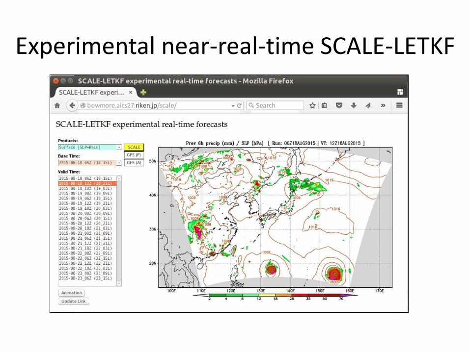
Experimental near-real-time SCALE-LETKF

• Domain: – Horizontal: 18-km resolution; 320 x 240 grids
– Vertical: 36 levels (0 ~ 29 km)
• 50 members.
• 6-hourly analysis cycle; 5-day forecasts from the ensemble mean.
• Observations: – NCEP PREPBUFR conventional (non-radiance)
observation data.
Experimental near-real-time SCALE-LETKF

Time frame
GFS analysis/ forecast ready
GDAS PREPBUFR ready (full version observations)
GFS PREPBUFR ready (early version observations;
~90% of the full version)
9h ens forecasts (-6 ~ +3h) + LETKF (0 h)
3:40 6:40 7:20 9:20 3:20
120h forecast (0 ~ +120h) from the ens mean
0:00
Real time
9:35
Plotting
400 node-hours
80 node-hours
(60,000 node-hours per month)

SCALE-LETKF analysis vs. GFS analysis
SCALE-LETKF analysis
GFS analysis

5 day forecast of Typhoon NANGKA (201511) stating at 12:00 UTC July 12
Topics in the internship program
My purpose: Learning a data assimilation system of an atmospheric model
-> Verification of the near-real-time analysis and forecast system -> Research on 2015 typhoon Nangka -- Sensitivities of the localization scales to TC track and intensity forecasts -- TC vital assimilation -- Ensemble forecasts and downscaling forecasts

Verification of the near-real-time analysis and forecast system
-> Average root-mean-square errors (RMSE) and biases over the 1.5 month period
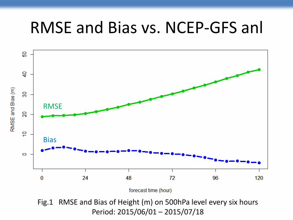
RMSE and Bias vs. NCEP-GFS anl
Fig.1 RMSE and Bias of Height (m) on 500hPa level every six hours Period: 2015/06/01 – 2015/07/18
RMSE
Bias

RMSE and Bias vs. NCEP-GFS anl
Fig.1 RMSE and Bias of Height (m) on 500hPa level every six hours Period: 2015/06/01 – 2015/07/18
Constantly increasing
Almost flat

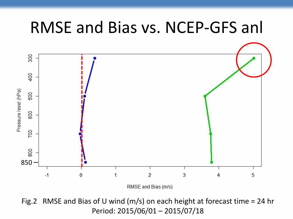
RMSE and Bias vs. NCEP-GFS anl
Fig.2 RMSE and Bias of U wind (m/s) on each height at forecast time = 24 hr Period: 2015/06/01 – 2015/07/18
RMSE Bias 850
RMSE and Bias vs. NCEP-GFS anl
Fig.2 RMSE and Bias of U wind (m/s) on each height at forecast time = 24 hr Period: 2015/06/01 – 2015/07/18
850
Summary of the verification
・The results of the near-real-time analysis and forecast system with the SCALE-LETKF are reasonable

Study on 2015 typhoon Nangka ・Background of the typhoon event
・Assimilation and forecast experiments (CTL)
・Sensitivity experiments -> Change horizontal localization parameter -> Change vertical localization parameter -> TC vital data assimilation
・Ensemble rainfall forecasts
・High resolution experiment
Background
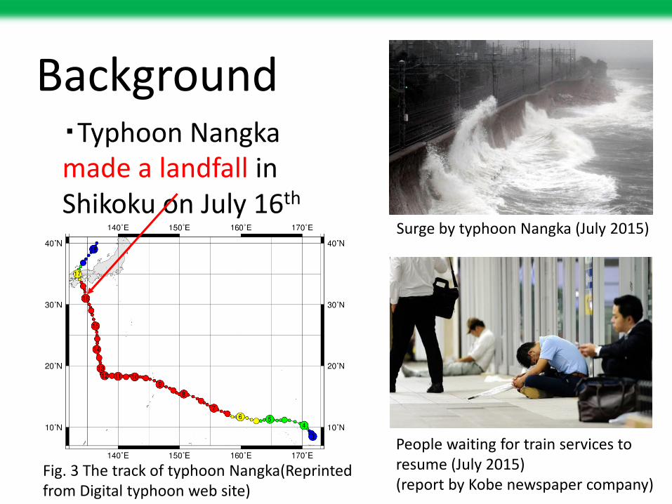
・Typhoon Nangka made a landfall in Shikoku on July 16th
Surge by typhoon Nangka (July 2015)
People waiting for train services to resume (July 2015) (report by Kobe newspaper company)
・Break a record of maximum daily precipitation on Kobe
Fig. 3 The track of typhoon Nangka(Reprinted from Digital typhoon web site)

Background
・Typhoon Nangka made a landfall in Shikoku on July 16th
Surge by typhoon Nangka (July 2015)
People waiting for train services to resume (July 2015) (report by Kobe newspaper company)
・Break a record of maximum daily precipitation at several spots

Distribution of the rainfall
Fig. 4 Distribution of accumulated precipitation from 13L Jul 15th to 13L Jul 18th by AMeDAS (Reprinted from http://www.jma-net.go.jp/osaka/kikou/saigai/pdf/sokuhou/20150718.pdf)

Time series of the rainfall in Hyogo
7/17 7/18
40
40
40
20
0
(mm)
0
0
0
400
400
400
400
(mm)
0
0
0
0
Fig.5 Time series of hourly precipitation at AMeDAS stations in Hyogo (Reprinted from http://www.jma-net.go.jp/osaka/kikou/saigai/pdf/sokuhou/20150718.pdf)

Overview of the control(CTRL) experiment
analysis 07/12/2015 ; 00Z
Time integration
guess 07/12/2015 ; 06Z
Five days forecast
07/12/2015 ; 12Z
analysis
Time integration
Two cycle assimilation
analysis
guess
Localization parameters : 𝜎 = 400km 𝜎v = 0.3ln𝑝

Overview of the CTRL experiment
analysis 07/12/2015 ; 00Z
Time integration
guess 07/12/2015 ; 06Z
Five days forecast
07/12/2015 ; 12Z
analysis
Time integration
Two cycle assimilation
analysis
guess
Localization parameters : 𝜎 = 400km 𝜎v = 0.3ln𝑝
boundary condition from GFS analysis
boundary condition from GFS analysis

Tracks in the CTRL experiment
MSLP (hPa)
○:Experiment
×:JMA Best_track
Fig.6 Typhoon tracks in the control run (circle) and the JMA best track data (cross)
0
200
400
600
Trac
k Er
rors
(km
)
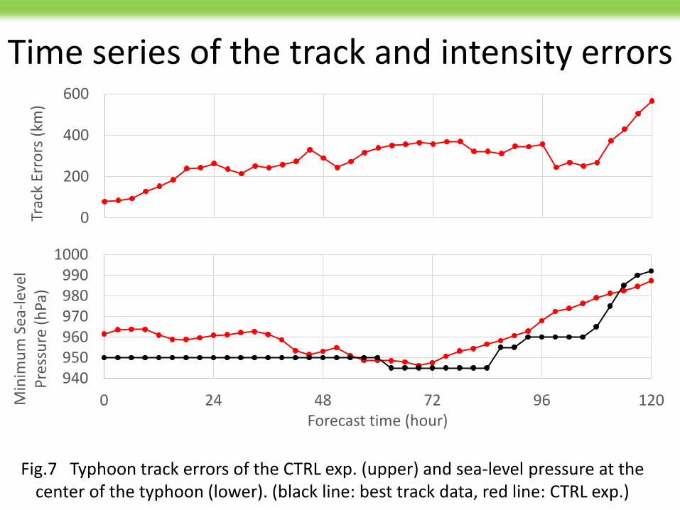
Time series of the track and intensity errors
940950960970980990
1000
0 24 48 72 96 120Min
imu
m S
ea-l
evel
P
ress
ure
(h
Pa)
Forecast time (hour)
Fig.7 Typhoon track errors of the CTRL exp. (upper) and sea-level pressure at the center of the typhoon (lower). (black line: best track data, red line: CTRL exp.)

0
200
400
600
Trac
k Er
rors
(km
)
Time series of the track and intensity errors
940950960970980990
1000
0 24 48 72 96 120Min
imu
m S
ea-l
evel
P
ress
ure
(h
Pa)
Forecast time (hour)
Fig.8 Typhoon track errors of the CTRL exp. (upper) and minimum sea-level pressure (lower). (black line: best track data, red line: CTRL exp.)
Period that the center is over the land
Almost flat

Overview of the sensitivity experiments
analysis 07/12/2015 ; 00Z
Time integration
guess 07/12/2015 ; 06Z
(analysis)’ analysis ……
Five days forecast
Change 𝜎 or 𝜎V
reference JMA best track data (Preliminary value)
guess (guess)’ 07/12/2015 ; 12Z
Time integration ……
analysis (analysis)’
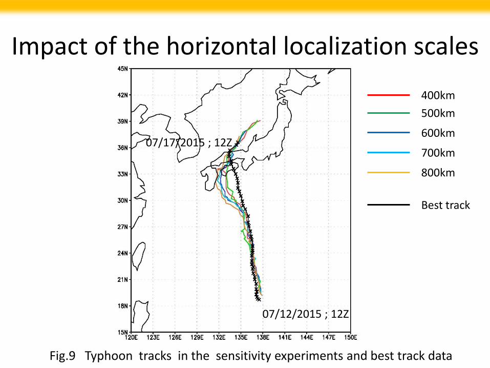
Impact of the horizontal localization scales
400km
500km
600km
700km
800km
Best track
07/12/2015 ; 12Z
07/17/2015 ; 12Z
Fig.9 Typhoon tracks in the sensitivity experiments and best track data

0
100
200
300
400
500
600
0 24 48 72 96 120
Trac
k Er
rors
(km
)
Forecast time (hour)
400km 500km 600km 700km 800km
The time series of track errors
2015071212Z
Fig.10 Typhoon tracks errors of the sensitivity experiments

930
940
950
960
970
980
990
1000
0 24 48 72 96 120
Min
imu
m S
ea-l
evel
Pre
ssu
re (
hPa
)
Forecast time (hour)
400km 500km 600km 700km 800km best_track
2015071212Z
Fig.11 Typhoon intensity of the sensitivity experiments
The time series of intensity

Impact of the vertical localization scales
0.1lnp
0.5lnp
0.1lnp
0.5lnp
Best track
400km
800km
07/12/2015 ; 12Z
07/17/2015 ; 12Z
Fig.12 Typhoon tracks in the sensitivity experiments and best track data
Control run 𝜎 = 400km 𝜎v = 0.3lnp

0
100
200
300
400
500
600
700
0 24 48 72 96 120
Trac
k Er
rors
(km
)
Forecast time (hour)
400km_0.1lnp 400km_0.5lnp 800km_0.1lnp
800km_0.5lnp control_run
The time series of track errors
2015071212Z
Fig.13 Typhoon tracks errors of the sensitivity experiments

930
940
950
960
970
980
990
1000
0 24 48 72 96 120
Sea-
leve
l Pre
ssu
re (
hPa
)
Forecast time (hour)
400km_0.1lnp 400km_0.5lnp 800km_0.1lnp
800km_0.5lnp best_track control_run
The time series of intensity
2015071212Z
Fig.14 Typhoon intensity of the sensitivity experiments

Summary of the sensitivity experiments
・Horizontal -> Changing horizontal localization scales has little impacts on the model results -> The trend of the track and intensity changes using from 400-km to 800-km localization scales is not very clear
・Vertical -> Changing vertical localization scales has also little impacts on the model results -> Track and intensity using 𝜎 = 400km, 𝜎v = 0.5ln𝑝 is similar to the control experiment

Introduce TC vital assimilation
• Initializing a representative vortex in the correct position and of appropriate intensity remains a serious challenge (Kleist, 2011; Wu et al. 2010; Kunii, 2015)
• A strategy for vortex initialization is TC vital assimilation
• In this case, we used minimum sea-level pressure(MSLP) and the position data as a TC vital data
• Tested only one cycle at 00Z 13th July 2015
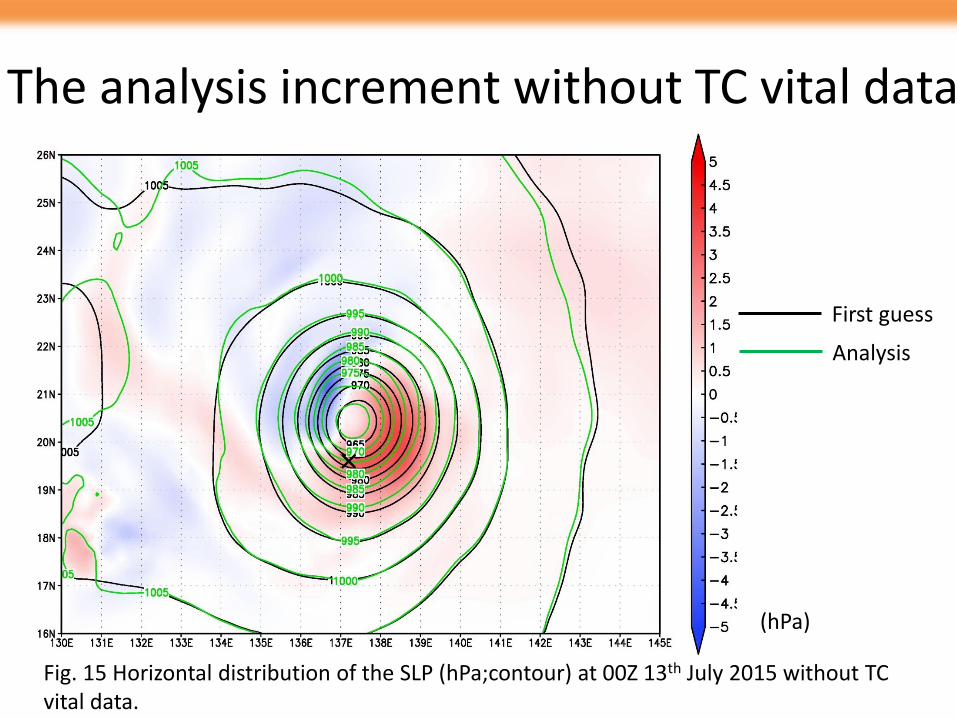
The analysis increment without TC vital data
Fig. 15 Horizontal distribution of the SLP (hPa;contour) at 00Z 13th July 2015 without TC vital data.
(hPa)
Analysis
First guess
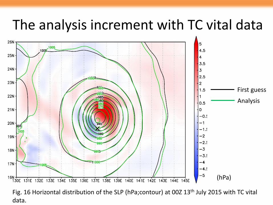
Fig. 16 Horizontal distribution of the SLP (hPa;contour) at 00Z 13th July 2015 with TC vital data.
(hPa)
Analysis
First guess
The analysis increment with TC vital data

The time series of track errors
0
50
100
150
200
250
300
350
400
450
500
0 24 48 72 96
Trac
k Er
rors
(km
)
Forecast time (hour)
without_TC_vital with_TC_vital
Fig.17 Typhoon tracks errors of the sensitivity experiments
2015071300Z

The time series of sea-level pressure
930
940
950
960
970
980
990
1000
1010
1020
0 24 48 72 96
Min
imu
m
Sea-
leve
l Pre
ssu
re (
hPa
)
Forecast time (hour)
without_TC_vital with_TC_vital best_track
Fig.18 Typhoon intensity of the sensitivity experiments
2015071300Z

The time series of sea-level pressure
930
940
950
960
970
980
990
1000
1010
1020
0 24 48 72 96
Min
imu
m S
ea-l
evel
Pre
ssu
re (
hPa
)
Forecast time (hour)
without_TC_vital with_TC_vital best_track
Fig.18 Typhoon intensity of the sensitivity experiments
2015071300Z

Summary of the TC vital assimilation
• The TC vital assimilation helps to move the TC center towards the observed location
• It also improves the track forecasts until 24 hours
Ensemble rainfall forecasts
• Motivation -> I’d like to investigate heavy rain by the typhoon Nangka in more detail. However, the SCALE model has not been implemented in cumulus parameterization.
• Purpose -> Investigating predictability of ensemble forecasts and the rainfall event by typhoon Nangka in Kobe.

Overview of the ensemble forecasts
Initial date 07/13/2015 ; 00Z
Carry out forecast experiment of all members
End date 07/18/2015 ; 00Z
48-hour rainfall
16Z;Jul15 to 15Z;Jul17
50
ensem
ble m
emb
ers

Fig.19 48-hour accumulated precipitation by JMA radar echo data (left) 48-hour accumulated precipitation in low resolution experiment (right)
Comparison of the result vs. obs.
[mm]
The Local maximum rainfall
JMA RADAR SCALE (ensemble mean)

Fig.20 Tracks of the result each member, ensemble mean, and JMA best track data
Ensemble mean
Each member
Best track

Fig.21 The center position of the typhoon each member at 16Z;Jul16th
The typhoon in the SCALE model has fast bias
Best track
The precipitation period should accelerate than that of the observation
16Z July 16th

Distinct four members
Fig.22 Disturibution of 48-hour accumulated rainfall of four each member
#31
#48 #21
#39

Fig.22 Probability about accumulated precipitation of getting beyond 200 [mm]
[%]
(15Z;Jul15 to 14Z;Jul17)

Fig.22 Probability about accumulated precipitation of getting beyond 200 [mm]
[%]
(15Z;Jul15 to 14Z;Jul17)
Very low probability
High-resolution (3km) forecasts experiment
・The 50-member near-real-time SCALE-LETKF is run at 18-km resolution, which is too low for simulating the local heavy rainfall event - The SCALE model does not have cumulus parameterization
・We run downscaling (offline nesting) forecasts at 3-km resolution based on one best (18-km resolution) member
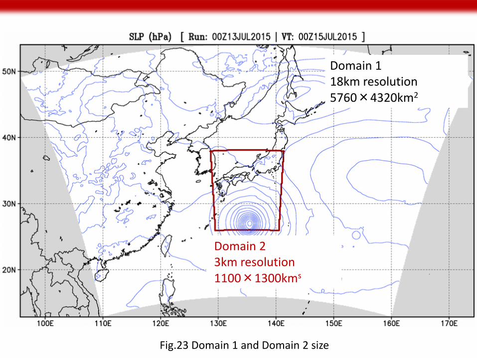
Domain 1 18km resolution 5760×4320km2
Domain 2 3km resolution 1100×1300kms
Fig.23 Domain 1 and Domain 2 size

Comparison between low-resolution and high-resolution model simulation
Fig.24 48-hour accumulated precipitation of high-resolution experiment is based on member 48 (right) and that of low resolution experiment (left)
MAX: 921.0 mm MAX: 533.9 mm

Comparison between observation and high-resolution model simulation
Fig.25 48-hour accumulated precipitation of high-resolution experiment is based on member 48 (right) and that of observation (left)
MAX: 921.0 mm MAX: 913.45 mm
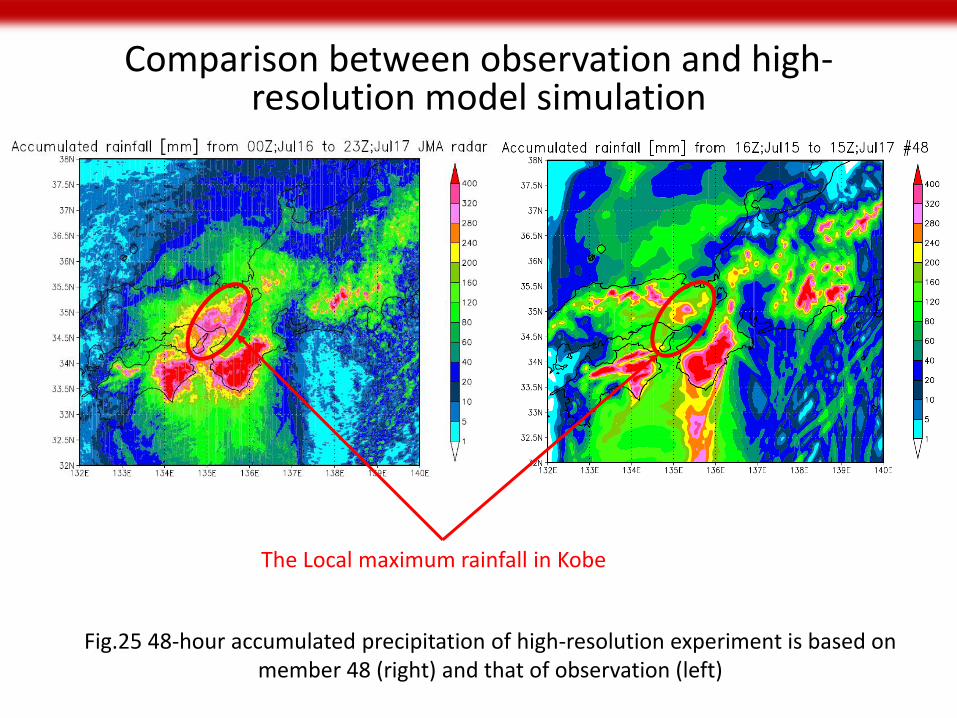
Comparison between observation and high-resolution model simulation
Fig.25 48-hour accumulated precipitation of high-resolution experiment is based on member 48 (right) and that of observation (left)
The Local maximum rainfall in Kobe

Summary of the ensemble forecasts and the high-resolution experiment
- The SCALE model can simulate the accumulated rainfall of this event reasonably well, but the local maximum rainfall near Kobe city is difficult to be predicted
- Ensemble forecasts shows large variability of the rainfall amounts and distributions even with the small track spread
- Probability forecast maps can be computed from the ensemble forecasts

Summary of the ensemble forecasts and the high-resolution experiment (cont.)
・3-km resolution forecast shows better results in both the distribution and the peak values of the accumulated rainfall - The rainfall peak near Kobe is better simulated in the high-resolution experiment, but still not perfect

Conclusion
・The SCALE-LETKF system operates correctly
・Changing localization parameter little impact on the model results
・A high-resolution forecast in SCALE model is able to represent a rainfall event more correctly

Thank you for your kind attention!