VELOCITY KINEMATICS – THE MANIPULATOR JACOBIANChapter 5 VELOCITY KINEMATICS – THE MANIPULATOR...

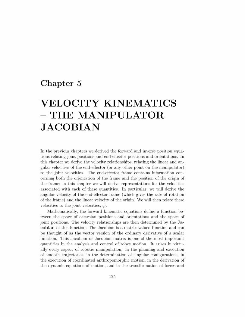
Chapter 5

VELOCITY KINEMATICS– THE MANIPULATORJACOBIAN

In the previous chapters we derived the forward and inverse position equa-tions relating joint positions and end-effector positions and orientations. Inthis chapter we derive the velocity relationships, relating the linear and an-gular velocities of the end-effector (or any other point on the manipulator)to the joint velocities. The end-effector frame contains information con-cerning both the orientation of the frame and the position of the origin ofthe frame; in this chapter we will derive representations for the velocitiesassociated with each of these quantities. In particular, we will derive theangular velocity of the end-effector frame (which gives the rate of rotationof the frame) and the linear velocity of the origin. We will then relate thesevelocities to the joint velocities, qi.

Mathematically, the forward kinematic equations define a function be-tween the space of cartesian positions and orientations and the space ofjoint positions. The velocity relationships are then determined by the Ja-

cobian of this function. The Jacobian is a matrix-valued function and canbe thought of as the vector version of the ordinary derivative of a scalarfunction. This Jacobian or Jacobian matrix is one of the most importantquantities in the analysis and control of robot motion. It arises in virtu-ally every aspect of robotic manipulation: in the planning and executionof smooth trajectories, in the determination of singular configurations, inthe execution of coordinated anthropomorphic motion, in the derivation ofthe dynamic equations of motion, and in the transformation of forces and

125

126CHAPTER 5. VELOCITY KINEMATICS – THE MANIPULATOR JACOBIAN

torques from the end-effector to the manipulator joints.

Since the Jacobian matrix encodes relationships between velocities, webegin this chapter with an investigation of velocities, and how to representthem. We first consider angular velocity about a fixed axis, and then gen-eralize this with the aid of skew symmetric matrices. Equipped with thisgeneral representation of angular velocities, we are able to derive equationsfor both the angular velocity, and the linear velocity for the origin, of amoving frame.

We then proceed to the derivation of the manipulator Jacobian. For an n-link manipulator we first derive the Jacobian representing the instantaneoustransformation between the n-vector of joint velocities and the 6-vector con-sisting of the linear and angular velocities of the end-effector. This Jacobianis then a 6 × n matrix. The same approach is used to determine the trans-formation between the joint velocities and the linear and angular velocityof any point on the manipulator. This will be important when we discussthe derivation of the dynamic equations of motion in Chapter 6. We thendiscuss the notion of singular configurations. These are configurations inwhich the manipulator loses one or more degrees-of-freedom. We show howthe singular configurations are determined geometrically and give severalexamples. Following this, we briefly discuss the inverse problems of deter-mining joint velocities and accelerations for specified end-effector velocitiesand accelerations. We end the chapter by considering redundant manipu-lators. This includes discussions of the inverse velocity problem, singularvalue decomposition and manipulability.

5.1 Angular Velocity: The Fixed Axis Case

When a rigid body moves in a pure rotation about a fixed axis, every pointof the body moves in a circle. The centers of these circles lie on the axis ofrotation. As the body rotates, a perpendicular from any point of the bodyto the axis sweeps out an angle θ, and this angle is the same for every pointof the body. If k is a unit vector in the direction of the axis of rotation,then the angular velocity is given by

ω = θk (5.1)

in which θ is the time derivative of θ.

Given the angular velocity of the body, one learns in introductory dy-namics courses that the linear velocity of any point on the body is given by

5.2. SKEW SYMMETRIC MATRICES 127

the equation

v = ω × r (5.2)

in which r is a vector from the origin (which in this case is assumed to lie onthe axis of rotation) to the point. In fact, the computation of this velocityv is normally the goal in introductory dynamics courses, and therefore, themain role of an angular velocity is to induce linear velocities of points in arigid body. In our applications, we are interested in describing the motionof a moving frame, including the motion of the origin of the frame throughspace and also the rotational motion of the frame’s axes. Therefore, for ourpurposes, the angular velocity will hold equal status with linear velocity.

As in previous chapters, in order to specify the orientation of a rigid ob-ject, we rigidly attach a coordinate frame to the object, and then specify theorientation of the coordinate frame. Since every point on the object experi-ences the same angular velocity (each point sweeps out the same angle θ in agiven time interval), and since each point of the body is in a fixed geometricrelationship to the body-attached frame, we see that the angular velocity isa property of the attached coordinate frame itself. Angular velocity is nota property of individual points. Individual points may experience a linearvelocity that is induced by an angular velocity, but it makes no sense tospeak of a point itself rotating. Thus, in equation (5.2) v corresponds tothe linear velocity of a point, while ω corresponds to the angular velocityassociated with a rotating coordinate frame.

In this fixed axis case, the problem of specifying angular displacements isreally a planar problem, since each point traces out a circle, and since everycircle lies in a plane. Therefore, it is tempting to use θ to represent theangular velocity. However, as we have already seen in Chapter 2, this choicedoes not generalize to the three-dimensional case, either when the axis ofrotation is not fixed, or when the angular velocity is the result of multiplerotations about distinct axes. For this reason, we will develop a more generalrepresentation for angular velocities. This is analogous to our development ofrotation matrices in Chapter 2 to represent orientation in three dimensions.The key tool that we will need to develop this representation is the skewsymmetric matrix, which is the topic of the next section.

5.2 Skew Symmetric Matrices

In the Section 5.3 we will derive properties of rotation matrices that canbe used to computing relative velocity transformations between coordinate


frames. Such transformations involve computing derivatives of rotation ma-trices. By introducing the notion of a skew symmetric matrix it is possibleto simplify many of the computations involved.

Definition 2 A matrix S is said to be skew symmetric if and only if

ST + S = 0. (5.3)

We denote the set of all 3 × 3 skew symmetric matrices by SS(3). If S ∈SS(3) has components sij , i, j = 1, 2, 3 then (5.3) is equivalent to the nineequations

sij + sji = 0 i, j = 1, 2, 3. (5.4)

From (5.4) we see that sii = 0; that is, the diagonal terms of S are zero andthe off diagonal terms sij , i 6= j satisfy sij = −sji. Thus S contains onlythree independent entries and every 3 × 3 skew symmetric matrix has theform

S =

0 −s3 s2s3 0 −s1−s2 s1 0

. (5.5)

If a = (ax, ay, az)T is a 3-vector, we define the skew symmetric matrix S(a)

as

S(a) =

0 −az ayaz 0 −ax−ay ax 0

. (5.6)

Example 5.1 We denote by i, j and k the three unit basis coordinatevectors,

i = (1, 0, 0)T

j = (0, 1, 0)T

k = (0, 0, 1)T .

The skew symmetric matrices S(i), S(j), and S(k) are given by

S(i) =

0 0 00 0 −10 1 0

; S(j) =

0 0 10 0 0

−1 0 0

; S(k) =

0 −1 01 0 00 0 0

.(5.7)

5.2. SKEW SYMMETRIC MATRICES 129

⋄

An important property possessed by the matrix S(a) is linearity. Forany vectors a and b belonging to IR3 and scalars α and β we have

S(αa + βb) = αS(a) + βS(b). (5.8)

Another important property of S(a) is that for any vector p = (px, py, pz)T

S(a)p = a × p (5.9)

where a×p denotes the vector cross product defined in Appendix A. Equa-tion (5.9) can be verified by direct calculation.

If R ∈ SO(3) and a, b are vectors in IR3 it can also be shown by directcalculation that

R(a × b) = Ra ×Rb. (5.10)

Equation (5.10) is not true in general unlessR is orthogonal. Equation (5.10)says that if we first rotate the vectors a and b using the rotation transforma-tion R and then form the cross product of the rotated vectors Ra and Rb,the result is the same as that obtained by first forming the cross producta × b and then rotating to obtain R(a × b).

For any R ∈ SO(3) and any b ∈ IR3, it follows from (5.9) and (5.10) that

RS(a)RTb = R(a ×RTb) (5.11)

= (Ra) × (RRTb) (5.12)

= (Ra) × b (5.13)

= S(Ra)b. (5.14)

Here, (5.12) follows because of (5.10), and (5.13) follows since R is orthogo-nal. Since this equality holds for all b ∈ IR3, we have shown the useful factthat

RS(a)RT = S(Ra) (5.15)

for R ∈ SO(3), a ∈ IR3. As we will see, (5.15) is one of the most usefulexpressions that we will derive. The left hand side of Equation (5.15) rep-resents a similarity transformation of the matrix S(a). The equation saystherefore that the matrix representation of S(a) in a coordinate frame ro-tated by R is the same as the skew symmetric matrix S(Ra) correspondingto the vector a rotated by R.


Suppose now that a rotation matrix R is a function of the single variableθ. Hence R = R(θ) ∈ SO(3) for every θ. Since R is orthogonal for all θ itfollows that

R(θ)R(θ)T = I. (5.16)

Differentiating both sides of (5.16) with respect to θ using the product rulegives

dR

dθR(θ)T +R(θ)

dRT

dθ= 0. (5.17)

Let us define the matrix

S :=dR

dθR(θ)T . (5.18)

Then the transpose of S is

ST =

(

dR

dθR(θ)T

)T

= R(θ)dRT

dθ. (5.19)

Equation (5.17) says therefore that

S + ST = 0. (5.20)

In other words, the matrix S defined by (5.18) is skew symmetric. Multiply-ing both sides of (5.18) on the right by R and using the fact that RTR = Iyields

dR

dθ= SR(θ). (5.21)

Equation (5.21) is very important. It says that computing the derivativeof the rotation matrix R is equivalent to a matrix multiplication by a skewsymmetric matrix S. The most commonly encountered situation is the casewhere R is a basic rotation matrix or a product of basic rotation matrices.

Example 5.2 If R = Rx,θ, the basic rotation matrix given by (2.19), thendirect computation shows that

S =dR

dθRT =

0 0 00 − sin θ − cos θ0 cos θ − sin θ

1 0 00 cos θ sin θ0 − sin θ cos θ

(5.22)

=

0 0 00 0 −10 1 0

= S(i). (5.23)

5.3. ANGULAR VELOCITY: THE GENERAL CASE 131

Thus we have shown that

dRx,θ

dθ= S(i)Rx,θ. (5.24)

Similar computations show that

dRy,θ

dθ= S(j)Ry,θ;

dRz,θ

dθ= S(k)Rz,θ. (5.25)

⋄

Example 5.3 Let Rk,θ be a rotation about the axis defined by k as in (2.71).Note that in this example k is not the unit coordinate vector (0, 0, 1)T . It iseasy to check that S(k)3 = −S(k). Using this fact together with Problem 12it follows that

dRk,θ

dθ= S(k)Rk,θ. (5.26)

⋄

5.3 Angular Velocity: The General Case

We now consider the general case of angular velocity about an arbitrary,possibly moving, axis. Suppose that a rotation matrix R is time varying, sothat R = R(t) ∈ SO(3) for every t ∈ IR. An argument identical to the onein the previous section shows that the time derivative R(t) of R(t) is givenby

R(t) = S(t)R(t) (5.27)

where the matrix S(t) is skew symmetric. Now, since S(t) is skew symmetric,it can be represented as S(ω(t)) for a unique vector ω(t). This vector ω(t) isthe angular velocity of the rotating frame with respect to the fixed frameat time t. Thus, the time derivative R(t) is given by

R(t) = S(ω(t))R(t) (5.28)

in which ω(t) is the angular velocity.

Example 5.4 Suppose that R(t) = Rx,θ(t). Then R(t) = dRdt is computed

using the chain rule as

R =dR

dθ

dθ

dt= θS(i)R(t) = S(ω(t))R(t) (5.29)

where ω = iθ is the angular velocity. Note, here i = (1, 0, 0)T .⋄


5.4 Addition of Angular Velocities

We are often interested in finding the resultant angular velocity due to therelative rotation of several coordinate frames. We now derive the expressionsfor the composition of angular velocities of two moving frames o1x1y1z1 ando2x2y2z2 relative to the fixed frame o0x0y0z0. For now, we assume that thethree frames share a common origin. Let the relative orientations of theframes o1x1y1z1 and o2x2y2z2 be given by the rotation matrices R0

1(t) andR1

2(t) (both time varying). As in Chapter 2,

R02(t) = R0

1(t)R12(t). (5.30)

Taking derivatives of both sides of (5.30) with respect to time yields

R02 = R0

1R12 +R0

1R12. (5.31)

Using (5.28), the term R02 on the left-hand side of (5.31) can be written

R02 = S(ω0

2)R02. (5.32)

In this expression, ω02 denotes the total angular velocity experienced by

frame o2x2y2z2. This angular velocity results from the combined rotationsexpressed by R0

1 and R12.

The first term on the right-hand side of (5.31) is simply

R01R

12 = S(ω0

a)R01R

12 = S(ω0

a)R02. (5.33)

Note that in this equation, ω0a denotes the angular velocity of frame o1x1y1z1

that results from the changing R01, and this angular velocity vector is ex-

pressed relative to the coordinate system o0x0y0z0.

Let us examine the second term on the right hand side of (5.31). Usingthe expression (5.15) we have

R01R

12 = R0

1S(ω1b)R

12 (5.34)

= R01S(ω1

b)R01

TR01R

12 = S(R0

1ω1b)R

01R

12

= S(R01ω

1b)R

02. (5.35)

Note that in this equation, ω1b denotes the angular velocity of frame o2x2y2z2

that corresponds to the changing R12, expressed relative to the coordinate

system o1x1y1z1. Thus, the product R01ω

1b expresses this angular velocity

relative to the coordinate system o0x0y0z0.

5.5. LINEAR VELOCITY OF A POINT ATTACHED TO A MOVING FRAME133

Now, combining the above expressions we have shown that

S(ω02)R

02 = {S(ω0

a) + S(R01ω

1b)}R

02. (5.36)

Since S(a) + S(b) = S(a + b), we see that

ω02 = ω0

a +R01ω

1b . (5.37)

In other words, the angular velocities can be added once they are expressedrelative to the same coordinate frame, in this case o0x0y0z0.

The above reasoning can be extended to any number of coordinate sys-tems. In particular, suppose that we are given

R0n = R0

1R12 · · ·R

n−1n . (5.38)

Although it is a slight abuse of notation, let us represent by ωi−1

i the angu-lar velocity due to the rotation given by Ri−1

i , expressed relative to frameoi−1xi−1yi−1zi−1. Extending the above reasoning we obtain

R0n = S(ω0

n)R0n (5.39)

where

ω0n = ω0

1 +R01ω

12 +R0

2ω23 +R0

3ω34 + · · · +R0

n−1ωn−1n . (5.40)

5.5 Linear Velocity of a Point Attached to a Mov-ing Frame

We now consider the linear velocity of a point that is rigidly attached to amoving frame. Suppose the point p is rigidly attached to the frame o1x1y1z1,and that o1x1y1z1 is rotating relative to the frame o0x0y0z0. Then thecoordinates of p with respect to the frame o0x0y0z0 are given by

p0 = R01(t)p

1. (5.41)

The velocity p0 is then given as

p0 = R01(t)p

1 +R01(t)p

1 (5.42)

= S(ω0)R01(t)p

1 (5.43)

= S(ω0)p0 = ω0 × p0

which is the familiar expression for the velocity in terms of the vector crossproduct. Note that (5.43) follows from that fact that p is rigidly attached


to frame o1x1y1z1, and therefore its coordinates relative to frame o1x1y1z1do not change, giving p1 = 0.

Now suppose that the motion of the frame o1x1y1z1 relative to o0x0y0z0is more general. Suppose that the homogeneous transformation relating thetwo frames is time-dependent, so that

H01 (t) =

[

R01(t) O0

1(t)0 1

]

. (5.44)

For simplicity we omit the argument t and the subscripts and super-scripts on R0

1 and O01, and write

p0 = Rp1 +O. (5.45)

Differentiating the above expression using the product rule gives

p0 = Rp1 + O (5.46)

= S(ω)Rp1 + O

= ω × r + v

where r = Rp1 is the vector from O1 to p expressed in the orientation of theframe o0x0y0z0, and v is the rate at which the origin O1 is moving.

If the point p is moving relative to the frame o1x1y1z1, then we must addto the term v the term R(t)p1, which is the rate of change of the coordinatesp1 expressed in the frame o0x0y0z0.

5.6 Derivation of the Jacobian

Consider an n-link manipulator with joint variables q1, . . . , qn . Let

T 0n(q) =

[

R0n(q) O0

n(q)0 1

]

(5.47)

denote the transformation from the end-effector frame to the base frame,where q = (q1, . . . , qn)

T is the vector of joint variables. As the robot movesabout, both the joint variables qi and the end-effector position O0

n and ori-entation R0

n will be functions of time. The objective of this section is torelate the linear and angular velocity of the end-effector to the vector ofjoint velocities q(t). Let

S(ω0n) = R0

n(R0n)T (5.48)

5.6. DERIVATION OF THE JACOBIAN 135

define the angular velocity vector ω0n of the end-effector, and let

v0n = O0

n (5.49)

denote the linear velocity of the end effector. We seek expressions of theform

v0n = Jvq (5.50)

ω0n = Jωq (5.51)

where Jv and Jω are 3 × n matrices. We may write (5.50) and (5.51)together as

[

v0n

ω0n

]

= J0nq (5.52)

where J0n is given by

J0n =

[

JvJω

]

. (5.53)

The matrix J0n is called the Manipulator Jacobian or Jacobian for short.

Note that J0n is a 6 × n matrix where n is the number of links. We next

derive a simple expression for the Jacobian of any manipulator.

5.6.1 Angular Velocity

Recall from Equation (5.40) that angular velocities can be added vectoriallyprovided that they are expressed relative to a common coordinate frame.Thus we can determine the angular velocity of the end-effector relative tothe base by expressing the angular velocity contributed by each joint in theorientation of the base frame and then summing these.

If the i-th joint is revolute, then the i-th joint variable qi equals θi andthe axis of rotation is zi−1. Following the convention that we introducedabove, let ωi−1

i represent the angular velocity of link i that is imparted bythe rotation of joint i, expressed relative to frame oi−1xi−1yi−1zi−1. Thisangular velocity is expressed in the frame i− 1 by

ωi−1

i = qizi−1

i−1 = qik (5.54)

in which, as above, k is the unit coordinate vector (0, 0, 1)T .


If the i-th joint is prismatic, then the motion of frame i relative to framei− 1 is a translation and

ωi−1

i = 0. (5.55)

Thus, if joint i is prismatic, the angular velocity of the end-effector does notdepend on qi, which now equals di.

Therefore, the overall angular velocity of the end-effector, ω0n, in the base

frame is determined by Equation (5.40) as

ω0n = ρ1q1k + ρ2q2R

01k + · · · + ρnqnR

0n−1k (5.56)

=n

∑

i−1

ρiqiz0i−1

in which ρi is equal to 1 if joint i is revolute and 0 if joint i is prismatic,since

z0i−1 = R0

i−1k. (5.57)

Of course z00 = k = (0, 0, 1)T .

The lower half of the Jacobian Jω, in (5.53) is thus given as

Jω = [ρ1z0 · · · ρnzn−1] . (5.58)

Note that in this equation, we have omitted the superscripts for the unitvectors along the z-axes, since these are all referenced to the world frame.In the remainder of the chapter we will follow this convention when there isno ambiguity concerning the reference frame.

5.6.2 Linear Velocity

The linear velocity of the end-effector is just O0n. By the chain rule for

differentiation

O0n =

n∑

i=1

∂O0n

∂qiqi. (5.59)

Thus we see that the i-th column of Jv, which we denote as Jviis given by

Jvi=∂O0

n

∂qi. (5.60)

Furthermore this expression is just the linear velocity of the end-effectorthat would result if qi were equal to one and the other qj were zero. Inother words, the i-th column of the Jacobian can be generated by holdingall joints fixed but the i-th and actuating the i-th at unit velocity. We nowconsider the two cases (prismatic and revolute joints) separately.


(i) Case 1: Prismatic Joints

If joint i is prismatic, then it imparts a pure translation to the end-effector.From our study of the DH convention in Chapter 3, we can write the T 0

n asthe product of three transformations as follows

[

R0n O0

n

0 1

]

= T 0n (5.61)

= T 0i−1T

i−1i T i

n (5.62)

=

[

R0i−1 O0

i−1

0 1

] [

Ri−1i Oi−1

i

0 1

] [

Rin Oi

n

0 1

]

(5.63)

=

[

R0n R0

iOin +R0

i−1Oi−1

i +O0i−1

0 1

]

, (5.64)

which gives

O0n = R0

iOi

n +R0i−1O

i−1

i +O0i−1. (5.65)

If only joint i is allowed to move, then both of Oin and O0

i−1 are constant.Furthermore, if joint i is prismatic, then the rotation matrix R0

i−1 is alsoconstant (again, assuming that only joint i is allowed to move). Finally,recall from Chapter 3 that, by the DH convention, Oi−1

i = (aici, aisi, di)T .

Thus, differentiation of O0n gives

∂O0n

∂qi=

∂

∂diR0

i−1Oi−1

i (5.66)

= R0i−1

∂

∂di

aiciaisidi

(5.67)

= diR0i−1

001

(5.68)

= diz0i−1, (5.69)

in which di is the joint variable for prismatic joint i. Thus, (again, droppingthe zero superscript on the z-axis) for the case of prismatic joints we have

Jvi= zi−1. (5.70)


(ii) Case 2: Revolute Joints

If joint i is revolute, then we have qi = θi. Starting with (5.65), and lettingqi = θi, since R0

i is not constant with respect to θi, we obtain

∂

∂θiO0n =

∂

∂θi

[

R0iO

i

n +R0i−1O

i−1

i

]

(5.71)

=∂

∂θiR0

iOi

n +R0i−1

∂

∂θiOi−1

i (5.72)

= θiS(z0i−1)R

0iO

i

n + θiS(z0i−1)R

0i−1O

i−1

i (5.73)

= θiS(z0i−1)

[

R0iO

i

n +R0i−1O

i−1

i

]

(5.74)

= θiS(z0i−1)(O

0n −O0

i−1) (5.75)

= θiz0i−1 × (O0

n −O0i−1). (5.76)

The second term in (5.73) is derived as follows:

R0i−1

∂

∂θi

aiciaisidi

= R0

i−1

−aisiaici0

θi (5.77)

= R0i−1S(kθi)O

i−1

i (5.78)

= R0i−1S(kθi)

(

R0i−1

)TR0

i−1Oi−1

i (5.79)

= S(R0i−1kθi)R

0i−1O

i−1

i (5.80)

= θiS(z0i−1)R

0i−1O

i−1

i . (5.81)

Equation (5.78) follows by straightforward computation. Thus

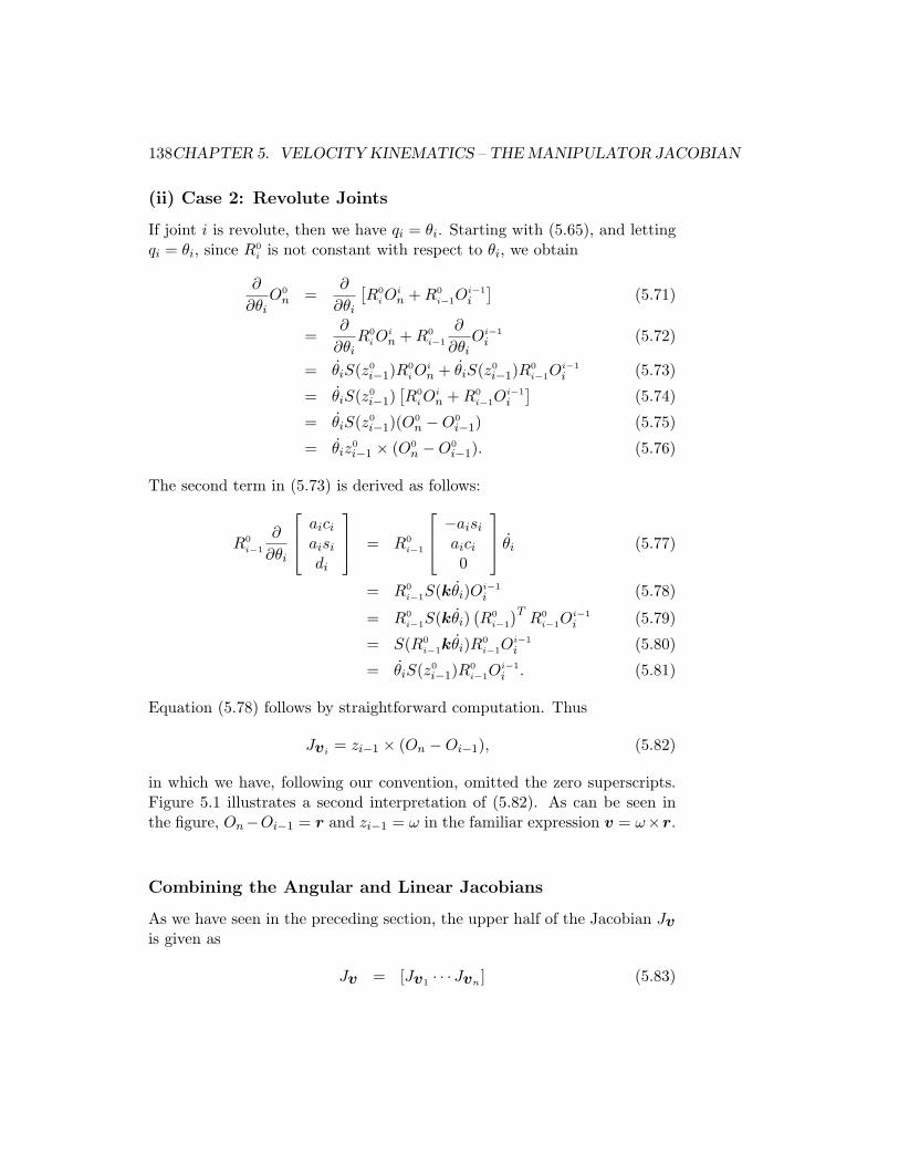
Jvi= zi−1 × (On −Oi−1), (5.82)

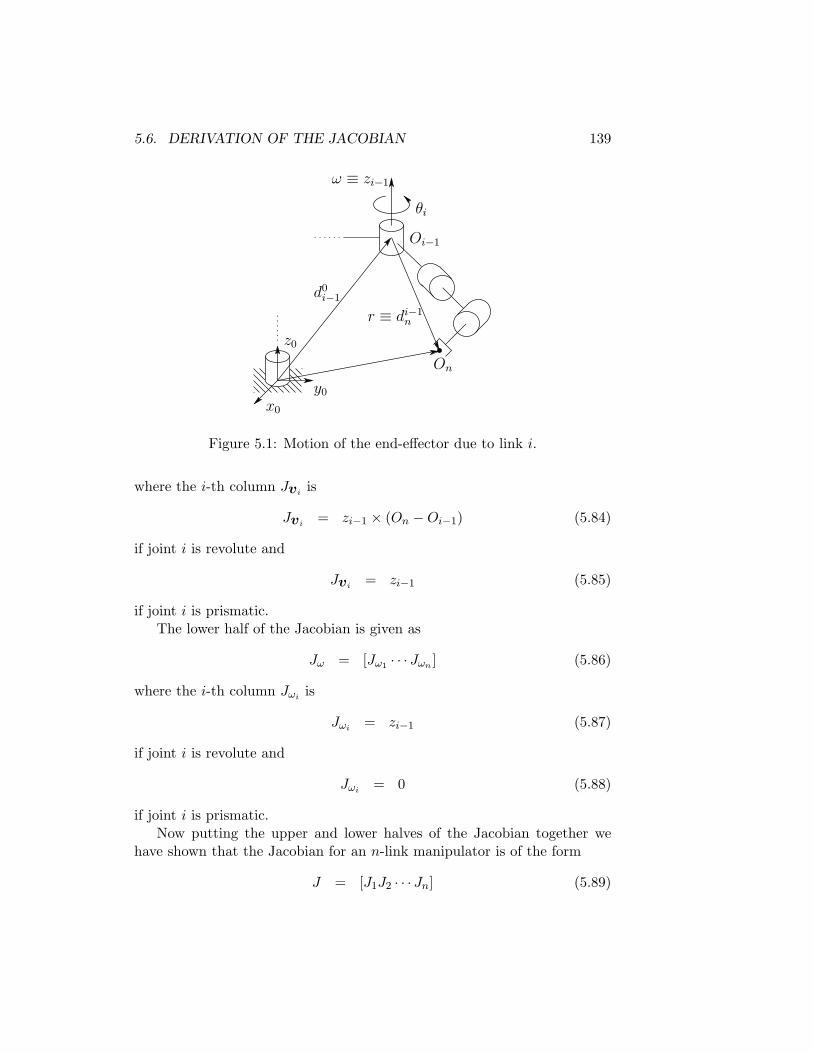
in which we have, following our convention, omitted the zero superscripts.Figure 5.1 illustrates a second interpretation of (5.82). As can be seen inthe figure, On−Oi−1 = r and zi−1 = ω in the familiar expression v = ω×r.

Combining the Angular and Linear Jacobians

As we have seen in the preceding section, the upper half of the Jacobian Jvis given as

Jv = [Jv1 · · ·Jvn ] (5.83)


Oi−1

y0

x0

z0

On

θi

d0

i−1

r ≡ di−1

n

ω ≡ zi−1

Figure 5.1: Motion of the end-effector due to link i.

where the i-th column Jviis

Jvi= zi−1 × (On −Oi−1) (5.84)

if joint i is revolute and

Jvi= zi−1 (5.85)

if joint i is prismatic.The lower half of the Jacobian is given as

Jω = [Jω1 · · ·Jωn ] (5.86)

where the i-th column Jωiis

Jωi= zi−1 (5.87)


Jωi= 0 (5.88)

if joint i is prismatic.Now putting the upper and lower halves of the Jacobian together we

have shown that the Jacobian for an n-link manipulator is of the form

J = [J1J2 · · ·Jn] (5.89)


where the i-th column Ji is given by

Ji =

[

zi−1 × (On −Oi−1)zi−1

]

(5.90)


Ji =

[

zi−1

0

]

(5.91)

if joint i is prismatic.

The above formulas make the determination of the Jacobian of any ma-nipulator simple since all of the quantities needed are available once theforward kinematics are worked out. Indeed the only quantities needed tocompute the Jacobian are the unit vectors zi and the coordinates of theorigins O1, . . . , On. A moment’s reflection shows that the coordinates for ziw.r.t. the base frame are given by the first three elements in the third col-umn of T 0

i while Oi is given by the first three elements of the fourth columnof T 0

i . Thus only the third and fourth columns of the T matrices are neededin order to evaluate the Jacobian according to the above formulas.

The above procedure works not only for computing the velocity of theend-effector but also for computing the velocity of any point on the manip-ulator. This will be important in Chapter 6 when we will need to computethe velocity of the center of mass of the various links in order to derive thedynamic equations of motion.

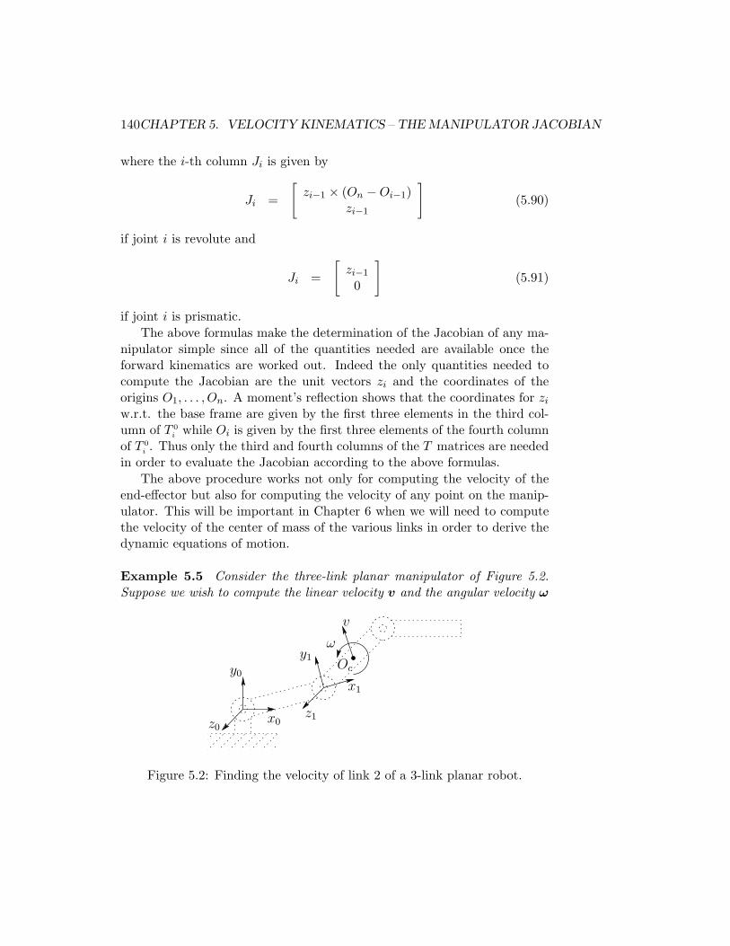
Example 5.5 Consider the three-link planar manipulator of Figure 5.2.Suppose we wish to compute the linear velocity v and the angular velocity ω

v

ω

z0x0

z1

x1

y0

y1

Oc

Figure 5.2: Finding the velocity of link 2 of a 3-link planar robot.

5.7. EXAMPLES 141

of the center of link 2 as shown. In this case we have that[

v

ω

]

= [J1 J2 J3]q (5.92)

where the columns of the Jacobian are determined using the above formulawith Oc in place of On. Thus we have

J1 = z0 × (Oc −O0) (5.93)

J2 = z1 × (Oc −O1)

and

J3 = 0

since the velocity of the second link is unaffected by motion of link 31. Notethat in this case the vector Oc must be computed as it is not given directlyby the T matrices (Problem 5-1).⋄

5.7 Examples

Example 5.6 Consider the two-link planar manipulator of Example 3.1.Since both joints are revolute the Jacobian matrix, which in this case is 6×2,is of the form

J(q) =

[

z0 × (O2 −O0) z1 × (O2 −O1)z0 z1

]

. (5.94)

The various quantities above are easily seen to be

O0 =

000

O1 =

a1c1a1s1

0

O2 =

a1c1 + a2c12a1s1 + a2s12

0

(5.95)

z0 = z1 =

001

. (5.96)

1Note that we are treating only kinematic effects here. Reaction forces on link 2 due to

the motion of link 3 will influence the motion of link 2. These dynamic effects are treated

by the methods of Chapter 6.


Performing the required calculations then yields

J =

−a1s1 − a2s12 −a2s12a1c1 + a2c12 a2c12

0 00 00 01 1

. (5.97)

It is easy to see how the above Jacobian compares with the expression(1.1) derived in Chapter 1. The first two rows of (5.96) are exactly the 2×2Jacobian of Chapter 1 and give the linear velocity of the origin O2 relativeto the base. The third row in (5.97) is the linear velocity in the direction ofz0, which is of course always zero in this case. The last three rows representthe angular velocity of the final frame, which is simply a rotation about thevertical axis at the rate θ1 + θ2.⋄Example 5.7 Stanford Manipulator Consider the Stanford manipulatorof Example 3.3.5 with its associated Denavit-Hartenberg coordinate frames.Note that joint 3 is prismatic and that O3 = O4 = O5 as a consequence ofthe spherical wrist and the frame assignment. Denoting this common originby O we see that the Jacobian is of the form

J =

[

z0 × (O6 −O0) z1 × (O6 −O1) z2 z3 × (O6 −O) z4 × (O6 −O) z5 × (O6 −O)z0 z1 0 z3 z4 z5

]

.

Now, using the A-matrices given by the expressions (3.35)-(3.40) andthe T -matrices formed as products of the A-matrices, these quantities areeasily computed as follows: First, Oj is given by the first three entries of thelast column of T 0

j = A1 · · ·Aj, with O0 = (0, 0, 0)T = O1. The vector zj isgiven as

zj = R0jk (5.98)

where R0j is the rotational part of T 0

j . Thus it is only necessary to computethe matrices T 0

j to calculate the Jacobian. Carrying out these calculationsone obtains the following expressions for the Stanford manipulator:

O6 = (dx, dy, dz)T =

c1s2d3 − s1d2 + d6(c1c2c4s5 + c1c5s2 − s1s4s5)s1s2d3 − c1d2 + d6(c1s4s5 + c2c4s1s5 + c5s1s2)

c2d3 + d6(c2c5 − c4s2s5)

(5.99)

O3 =

c1s2d3 − s1d2

s1s2d3 + c1d2

c2d3

. (5.100)

5.7. EXAMPLES 143

The zi are given as

z0 =

001

z1 =

−s1c10

(5.101)

z2 =

c1s2s1s2c2

z3 =

c1s2s1s2c2

(5.102)

z4 =

−c1c2s4 − s1c4−s1c2s4 + c1c4

s2s4

(5.103)

z5 =

c1c2c4s5 − s1s4s5 + c1s2c5s1c2c4s5 + c1s4s5 + s1s2c5

−s2c4s5 + c2c5

. (5.104)

The Jacobian of the Stanford Manipulator is now given by combiningthese expressions according to the given formulae (Problem 7).

⋄Example 5.8 SCARA Manipulator We will now derive the Jacobian ofthe SCARA manipulator of Example 3.3.6. This Jacobian is a 6× 4 matrixsince the SCARA has only four degrees-of-freedom. As before we need onlycompute the matrices T 0

j = A1 . . . Aj, where the A-matrices are given by(3.45)-(3.48).

Since joints 1,2, and 4 are revolute and joint 3 is prismatic, and sinceO4 −O3 is parallel to z3 (and thus, z3 × (O4 −O3) = 0), the Jacobian is ofthe form

J =

[

z0 × (O4 −O0) z1 × (O4 −O1) z2 0z0 z1 0 z3

]

. (5.105)

Performing the indicated calculations, one obtains

O1 =

a1c1a1s1

0

O2 =

a1c1 + a2c12a1s1 + a2s12

0

(5.106)

O4 =

a1c1 + a2c12a1s2 + a2s12d3 − d4

. (5.107)


Similarly z0 = z1 = k, and z2 = z3 = −k. Therefore the Jacobian of theSCARA Manipulator is

J =

−a1s1 − a2s12 −a2s12 0 0a1c1 + a2c12 a2c12 0 0

0 0 −1 00 0 0 00 0 0 01 1 0 −1

. (5.108)

⋄

5.8 Singularities

The 6 × n Jacobian J(q) defines a mapping

X = J(q)q (5.109)

between the vector q of joint velocities and the vector X = (v,ω)T of end-effector velocities. Infinitesimally this defines a linear transformation

dX = J(q)dq (5.110)

between the differentials dq and dX. These differentials may be thought ofas defining directions in IR6, and IRn, respectively.

Since the Jacobian is a function of the configuration q, those configu-rations for which the rank of J decreases are of special significance. Suchconfigurations are called singularities or singular configurations. Iden-tifying manipulator singularities is important for several reasons.

1. Singularities represent configurations from which certain directions ofmotion may be unattainable.

2. At singularities, bounded end-effector velocities may correspond to un-bounded joint velocities.

3. At singularities, bounded end-effector forces and torques may correspondto unbounded joint torques. (We will see this in Chapter ??).

4. Singularities usually (but not always) correspond to points on the bound-ary of the manipulator workspace, that is, to points of maximum reachof the manipulator.

5.8. SINGULARITIES 145

5. Singularities correspond to points in the manipulator workspace that maybe unreachable under small perturbations of the link parameters, suchas length, offset, etc.

6. Near singularities there will not exist a unique solution to the inversekinematics problem. In such cases there may be no solution or theremay be infinitely many solutions.

Example 5.9 Consider the two-dimensional system of equations

dX = Jdq =

[

1 10 0

]

dq (5.111)

that corresponds to the two equations

dx = dq1 + dq2 (5.112)

dy = 0. (5.113)

In this case the rank of J is one and we see that for any values of thevariables dq1 and dq2 there is no change in the variable dy. Thus any vectordX having a nonzero second component represents an unattainable directionof instantaneous motion.

⋄

5.8.1 Decoupling of Singularities

We saw in Chapter 3 that a set of forward kinematic equations can be de-rived for any manipulator by attaching a coordinate frame rigidly to eachlink in any manner that we choose, computing a set of homogeneous trans-formations relating the coordinate frames, and multiplying them togetheras needed. The D-H convention is merely a systematic way to do this.Although the resulting equations are dependent on the coordinate frameschosen, the manipulator configurations themselves are geometric quantities,independent of the frames used to describe them. Recognizing this fact al-lows us to decouple the determination of singular configurations, for thosemanipulators with spherical wrists, into two simpler problems. The firstis to determine so-called arm singularities, that is, singularities resultingfrom motion of the arm, which consists of the first three or more links, whilethe second is to determine the wrist singularities resulting from motionof the spherical wrist.


For the sake of argument, suppose that n = 6, that is, the manipulatorconsists of a 3-DOF arm with a 3-DOF spherical wrist. In this case theJacobian is a 6 × 6 matrix and a configuration q is singular if and only if

det J(q) = 0. (5.114)

If we now partition the Jacobian J into 3 × 3 blocks as

J = [JP | JO] =

[

J11

J21

J12

J22

]

(5.115)

then, since the final three joints are always revolute

JO =

[

z3 × (O6 −O3) z4 × (O6 −O4) z5 × (O6 −O5)z3 z4 z5

]

.(5.116)

Since the wrist axes intersect at a common point O, if we choose thecoordinate frames so that O3 = O4 = O5 = O6 = O, then JO becomes

JO =

[

0 0 0z3 z4 z5

]

(5.117)

and the i-th column Ji of Jp is

Ji =

[

zi−1 × (O −Oi−1)zi−1

]

(5.118)


Ji =

[

zi−1

0

]

(5.119)

if joint i is prismatic. In this case the Jacobian matrix has the block trian-gular form

J =

[

J11 0J21 J22

]

(5.120)

with determinant

det J = detJ11 det J22 (5.121)


where J11 and J22 are each 3× 3 matrices. J11 has i-th column zi−1 × (O−Oi−1) if joint i is revolute, and zi−1 if joint i is prismatic, while

J22 = [z3 z4 z5]. (5.122)

Therefore the set of singular configurations of the manipulator is theunion of the set of arm configurations satisfying detJ11 = 0 and the setof wrist configurations satisfying detJ22 = 0. Note that this form of theJacobian does not necessarily give the correct relation between the velocityof the end-effector and the joint velocities. It is intended only to simplifythe determination of singularities.

5.8.2 Wrist Singularities

We can now see from (5.122) that a spherical wrist is in a singular configu-ration whenever the vectors z3, z4 and z5 are linearly dependent. Referringto Figure 5.3 we see that this happens when the joint axes z3 and z5 are

z4

θ6θ4

θ5 = 0

z3 z5

Figure 5.3: Spherical wrist singularity.

collinear. In fact, whenever two revolute joint axes anywhere are collinear,a singularity results since an equal and opposite rotation about the axesresults in no net motion of the end-effector. This is the only singularity ofthe spherical wrist, and is unavoidable without imposing mechanical limitson the wrist design to restrict its motion in such a way that z3 and z5 areprevented from lining up.

5.8.3 Arm Singularities

In order to investigate arm singularities we need only to compute J11 ac-cording to (5.118) and (5.119), which is the same formula derived previouslywith the wrist center O in place of O6.


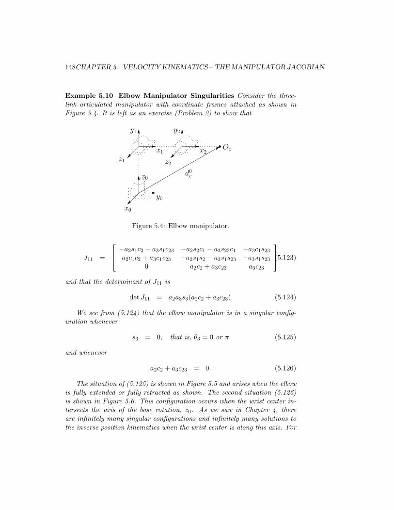
Example 5.10 Elbow Manipulator Singularities Consider the three-link articulated manipulator with coordinate frames attached as shown inFigure 5.4. It is left as an exercise (Problem 2) to show that

z2

x0

z0

x1 x2

z1

y1 y2

y0

Oc

d0

c

Figure 5.4: Elbow manipulator.

J11 =

−a2s1c2 − a3s1c23 −a2s2c1 − a3s23c1 −a3c1s23a2c1c2 + a3c1c23 −a2s1s2 − a3s1s23 −a3s1s23

0 a2c2 + a3c23 a3c23

(5.123)

and that the determinant of J11 is

det J11 = a2a3s3(a2c2 + a3c23). (5.124)

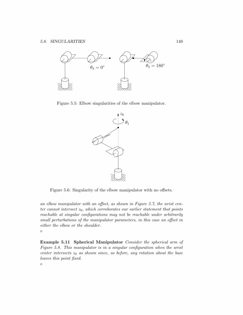
We see from (5.124) that the elbow manipulator is in a singular config-uration whenever

s3 = 0, that is, θ3 = 0 or π (5.125)

and whenever

a2c2 + a3c23 = 0. (5.126)

The situation of (5.125) is shown in Figure 5.5 and arises when the elbowis fully extended or fully retracted as shown. The second situation (5.126)is shown in Figure 5.6. This configuration occurs when the wrist center in-tersects the axis of the base rotation, z0. As we saw in Chapter 4, thereare infinitely many singular configurations and infinitely many solutions tothe inverse position kinematics when the wrist center is along this axis. For


θ3 = 0◦ θ3 = 180

◦

Figure 5.5: Elbow singularities of the elbow manipulator.

z0

θ1

Figure 5.6: Singularity of the elbow manipulator with no offsets.

an elbow manipulator with an offset, as shown in Figure 5.7, the wrist cen-ter cannot intersect z0, which corroborates our earlier statement that pointsreachable at singular configurations may not be reachable under arbitrarilysmall perturbations of the manipulator parameters, in this case an offset ineither the elbow or the shoulder.

⋄

Example 5.11 Spherical Manipulator Consider the spherical arm ofFigure 5.8. This manipulator is in a singular configuration when the wristcenter intersects z0 as shown since, as before, any rotation about the baseleaves this point fixed.

⋄


z0

d

Figure 5.7: Elbow manipulator with shoulder offset.

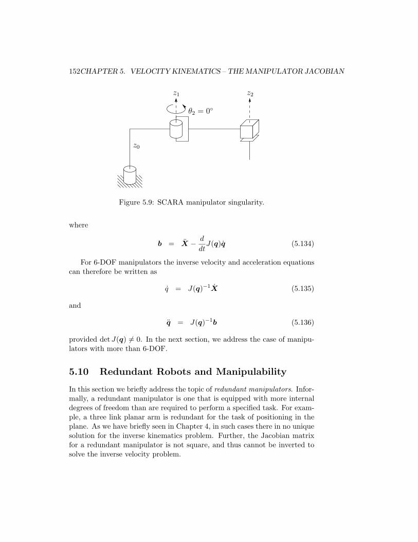
Example 5.12 SCARA Manipulator We have already derived the com-plete Jacobian for the the SCARA manipulator. This Jacobian is simpleenough to be used directly rather than deriving the modified Jacobian fromthis section. Referring to Figure 5.9 we can see geometrically that the onlysingularity of the SCARA arm is when the elbow is fully extended or fullyretracted. Indeed, since the portion of the Jacobian of the SCARA governingarm singularities is given as

J11 =

α1 α3 0α2 α4 00 0 −1

(5.127)

where

α1 = −a1s1 − a2s12 (5.128)

α2 = a1c1 + a2c12

α3 = −a1s12

α4 = a1c12 (5.129)

we see that the rank of J11 will be less than three precisely whenever α1α4 −α2α3 = 0. It is easy to compute this quantity and show that it is equivalentto (Problem 4)

s2 = 0, which implies θ2 = 0, π. (5.130)

5.9. INVERSE VELOCITY AND ACCELERATION 151

θ1

z0

Figure 5.8: Singularity of spherical manipulator with no offsets.

⋄

5.9 Inverse Velocity and Acceleration

It is perhaps a bit surprising that the inverse velocity and acceleration rela-tionships are conceptually simpler than inverse position. Recall from (5.109)that the joint velocities and the end-effector velocities are related by the Ja-cobian as

X = J(q)q. (5.131)

Thus the inverse velocity problem becomes one of solving the system oflinear equations (5.131), which is conceptually simple.

Differentiating (5.131) yields the acceleration equations

X = J(q)q +

(

d

dtJ(q)

)

q. (5.132)

Thus, given a vector X of end-effector accelerations, the instantaneousjoint acceleration vector q is given as a solution of

b = J(q)q (5.133)


z0

z1 z2

θ2 = 0◦

Figure 5.9: SCARA manipulator singularity.

where

b = X −d

dtJ(q)q (5.134)

For 6-DOF manipulators the inverse velocity and acceleration equationscan therefore be written as

q = J(q)−1X (5.135)

and

q = J(q)−1b (5.136)

provided detJ(q) 6= 0. In the next section, we address the case of manipu-lators with more than 6-DOF.

5.10 Redundant Robots and Manipulability

In this section we briefly address the topic of redundant manipulators. Infor-mally, a redundant manipulator is one that is equipped with more internaldegrees of freedom than are required to perform a specified task. For exam-ple, a three link planar arm is redundant for the task of positioning in theplane. As we have briefly seen in Chapter 4, in such cases there in no uniquesolution for the inverse kinematics problem. Further, the Jacobian matrixfor a redundant manipulator is not square, and thus cannot be inverted tosolve the inverse velocity problem.

5.10. REDUNDANT ROBOTS AND MANIPULABILITY 153

In this section, we begin by giving a brief and general introduction tothe subject of redundant manipulators. We then turn our attention to theinverse velocity problem. To address this problem, we will introduce theconcept of a pseudoinverse and the Singular Value Decomposition. We endthe section by introducing manipulability, a measure that can be used toquantify the quality of the internal configuration of a manipulator, and cantherefore be used in an optimization framework to aid in the solution forthe inverse kinematics problem.

5.10.1 Redundant Manipulators

A precise definition of what is meant by the term redundant requires thatwe specify a task, and the number of degrees of freedom required to performthat task. In previous chapters, we have dealt primarily with positioningtasks. In these cases, the task was determined by specifying the position,orientation or both for the end effector or some tool mounted at the endeffector. For these kinds of positioning tasks, the number of degrees offreedom for the task is equal to the number of parameters required to specifythe position and orientation information. For example, if the task involvespositioning the end effector in a 3D workspace, then the task can be specifiedby an element of ℜ3 × SO(3). As we have seen in Chapter 2, ℜ3 × SO(3)can be parameterized by (x, y, z, φ, θ, ψ), i.e., using six parameters. Thus,for this task, the task space is six-dimensional. A manipulator is said tobe redundant when its number of internal degrees of freedom (or joints) isgreater than the dimension of the task space. Thus, for the 3D positionand orientation task, any manipulator with more than six joints would beredundant.

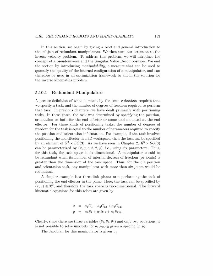
A simpler example is a three-link planar arm performing the task ofpositioning the end effector in the plane. Here, the task can be specified by(x, y) ∈ ℜ2, and therefore the task space is two-dimensional. The forwardkinematic equations for this robot are given by

x = a1C1 + a2C12 + a3C123

y = a1S1 + a2S12 + a3S123.

Clearly, since there are three variables (θ1, θ2, θ3) and only two equations, itis not possible to solve uniquely for θ1, θ2, θ3 given a specific (x, y).

The Jacobian for this manipulator is given by


J =

[

−a1S1 − a2S12 −a2S12 −a3S123

a1C1 + a2C12 a2C12 a3C123

]

. (5.137)

When using the relationship x = Jq to for q, we have a system of two linearequations in three unknowns. Thus there are also infinitely many solutionsto this system, and the inverse velocity problem cannot be solved uniquely.We now turn our attention to the specifics of dealing with these inverseproblems.

5.10.2 The Inverse Velocity Problem for Redundant Manip-ulators

We have seen in Section 5.9 that the inverse velocity problem is easily solvedwhen the Jacobian is square with nonzero determinant. However, whenthe Jacobian is not square, as is the case for redundant manipulators, themethod of Section 5.9 cannot be used, since a nonsquare matrix cannot beinverted. To deal with the case when m < n, we use the following resultfrom linear algebra.

Proposition: For J ∈ ℜm×n, if m < n and rank J = m, then (JJT )−1

exists.

In this case (JJT ) ∈ ℜm×m, and has rank m. Using this result, we canregroup terms to obtain

(JJT )(JJT )−1 = I

J[

JT (JJT )−1]

= I

JJ+ = I.

Here, J+ = JT (JJT )−1 is called a right pseudoinverse of J, since JJ+ = I.Note that, J+J ∈ ℜn×n, and that in general, J+J 6= I (recall that matrixmultiplication is not commutative).

It is now easy to demonstrate that a solution to (5.131) is given by

q = J+x + (I − J+J)b (5.138)

in which b ∈ ℜn is an arbitrary vector. To see this, multiply this solutionby J:

Jq = J [J+x + (I − J+J)b]

= JJ+x + J(I − J+J)b


= JJ+x + (J − JJ+J)b

= x + (J − J)b

= x.

In general, for m < n, (I − J+J) 6= 0, and all vectors of the form(I−J+J)b lie in the null space of J, i.e., if qn is a joint velocity vector suchthat qn = (I− J+J)b, then when the joints move with velocity qn, the endeffector will remain fixed since Jqn = 0. Thus, if q is a solution to (5.131),then so is q + qn with qn = (I− J+J)b, for any value of b. If the goal is tominimize the resulting joint velocities, we choose b = 0. To see this, applythe triangle inequality to obtain

|| q || = || J+x + (I − J+J)b ||

≤ || J+x || + || (I − J+J)b ||.

5.10.3 Singular Value Decomposition (SVD)

For robots that are not redundant, the Jacobian matrix is square, and wecan use tools such as the determinant, eigenvalues and eigenvectors to ana-lyze its properties. However, for redundant robots, the Jacobian matrix isnot square, and these tools simply do not apply. Their generalizations arecaptured by the Singular Value Decomposition (SVD) of a matrix, which wenow introduce.

As we described above, for J ∈ ℜm×n, we have JJT ∈ ℜm×m. Thissquare matrix has eigenvalues and eigenvectors that satisfy

JJTui = λiui (5.139)

in which λi and ui are corresponding eigenvalue and eigenvector pairs forJJT . We can rewrite this equation to obtain

JJTui − λiui = 0

(JJT − λiI)ui = 0. (5.140)

The latter equation implies that the matrix (JJT − λiI) is singular, and wecan express this in terms of its determinant as

det(JJT − λiI) = 0. (5.141)

We can use (5.141) to find the eigenvalues λ1 ≥ λ2 · · · ≥ λm ≥ 0 for JJT .The singular values for the Jacobian matrix J are given by the square rootsof the eigenvalues of JJT ,

σi =√

λi. (5.142)


The singular value decomposition of the matrix J is then given by

J = UΣVT , (5.143)

in which

U = [u1u2 . . .um] , V = [v1v2 . . .vn] (5.144)

are orthogonal matrices, and Σ ∈ Rm×n.

Σ =

σ1

σ2

..σm

∣

∣

∣

∣

∣

∣

∣

∣

∣

∣

∣

0

. (5.145)

We can compute the SVD of J as follows. We begin by finding thesingular values, σi, of J using (5.141) and (5.142). These singular valuescan then be used to find the eigenvectors u1, · · ·um that satisfy

JJTui = σ2i ui. (5.146)

These eigenvectors comprise the matrix U = [u1u2 . . .um]. The system ofequations (5.146) can be written as

JJTU = UΣ2m (5.147)

if we define the matrix Σm as

Σm =

σ1

σ2

..σm

.

Now, define

Vm = JTUΣ−1m (5.148)

and let V be any orthogonal matrix that satisfies V = [Vm | Vn−m] (notethat here Vn−m contains just enough columns so that the matrix V is ann×n matrix). It is a simple matter to combine the above equations to verify


(5.143):

UΣVT = U [Σm | 0]

[

VTm

VTn−m

]

(5.149)

= UΣmVTm (5.150)

= UΣm

(

JTUΣ−1m

)T(5.151)

= UΣm(Σ−1m )TUTJ (5.152)

= UΣmΣ−1m UTJ (5.153)

= UUTJ (5.154)

= J. (5.155)

Here, (5.149) follows immediately from our construction of the matricesU, V and Σm. Equation (5.151) is obtained by substituting (5.148) into(5.150). Equation (5.153) follows because Σ−1

m is a diagonal matrix, andthus symmetric. Finally, (5.155) is obtained using the fact that UT = U−1,since U is orthogonal.

It is a simple matter construct the right pseudoinverse of J using theSVD,

J+ = VΣ+UT

in which

Σ+ =

σ−11

σ−12

..σ−1m

∣

∣

∣

∣

∣

∣

∣

∣

∣

∣

∣

0

T

.

5.10.4 Manipulability

For a specific value of q, the Jacobian relationship defines the linear systemgiven by x = Jq. We can think of J a scaling the input, q, to producethe output, x. It is often useful to characterize quantitatively the effects ofthis scaling. Often, in systems with a single input and a single output, thiskind of characterization is given in terms of the so called impulse responseof a system, which essentially characterizes how the system responds toa unit input. In this multidimensional case, the analogous concept is tocharacterize the output in terms of an input that has unit norm. Considerthe set of all robot tool velocities q such that

‖q‖ = (q21 + q22 + . . . q2m)1/2 ≤ 1. (5.156)


If we use the minimum norm solution q = J+x, we obtain

‖q‖ = qT q

= (J+x)TJ+x

= xT (J+)TJ+x

= xT (JT (JJT )−1)TJT (JJT )−1x

= xT [(JJT )−1]TJJT (JJT )−1x

= xT (JJT )−1x ≤ 1. (5.157)

This final inequality gives us a quantitative characterization of the scalingthat is effected by the Jacobian. In particular, if the manipulator Jacobianis full rank, i.e., rank J = m, then (5.157) defines an m-dimensional ellipsoidthat is known as the manipulability ellipsoid. If the input (i.e., joint velocity)vector has unit norm, then the output (i.e., task space velocity) will lie withinthe ellipsoid given by (5.157). We can more easily see that (5.157) definesan ellipsoid by replacing J by its SVD to obtain

xT (JJT )−1xT = xT [UΣVT (UΣVT )T ]−1x

= xT [UΣVTVΣTUT ]−1x

= xT [UΣΣTUT ]−1x

= xT [UΣ2mUT ]−1x

= xT [UΣ−2m UT ]x

= (xTU)Σ−2m (UT x)

= (UT x)TΣ−2m (UT x) (5.158)

in which

Σ−2m =

σ−21

σ−22

..σ−2m

.

If we make the substation w = UT x, then (5.158) can be written as

wTΣ−2m w =

∑

σ−2i w2

i ≤ 1 (5.159)

and it is clear that this is the equation for an axis-aligned ellipse in a newcoordinate system that is obtained by rotation according to the orthogonalmatrix U. In the original coordinate system, the axes of the ellipsoid aregiven by the vectors σiui. The volume of the ellipsoid is given by

volume = Kσ1σ2 · · ·σm,


in which K is a constant that depends only on the dimension, m, of theellipsoid. The manipulability measure, as defined by Yoshikawa [?], is givenby

ω = σ1σ2 · · ·σm. (5.160)

Note that the constant K is not included in the definition of manipulability,since it is fixed once the task has been defined (i.e., once the dimension ofthe task space has been fixed).

Now, consider the special case that the robot is not redundant, i.e.,J ∈ ℜm×m. Recall that the determinant of a product is equal to the productof the determinants, and that a matrix and its transpose have the samedeterminant. Thus, we have

det JJT = det J det JT

= det J det J

= (λ1λ2 · · ·λm)(λ1λ2 · · ·λm)

= λ21λ

22 · · ·λ

2m (5.161)

in which λ1 ≥ λ2 · · · ≤ λm are the eigenvalues of J. This leads to

ω =√

det JJT = |λ1λ2 · · ·λm| = |det J|. (5.162)

The manipulability, ω, has the following properties.

• In general, ω = 0 holds if and only if rank(J) < m, (i.e., when J is notfull rank).

• Suppose that there is some error in the measured velocity, ∆x. Wecan bound the corresponding error in the computed joint velocity, ∆q,by

(σ1)−1 ≤

||∆q||

||∆x||≤ (σm)−1. (5.163)

Example 5.13 Two-link Planar Arm. We can use manipulability todetermine the optimal configurations in which to perform certain tasks. Insome cases it is desirable to perform a task in the configuration for whichthe end effector has the maximum dexterity. We can use manipulability asa measure of dexterity. Consider the two-link planar arm and the task ofpositioning in the plane. For the two link arm, the Jacobian is given by

J =

[

−a1S1 − a2S12 −a2S12

a1C1 + a2C12 a2C12

]

. (5.164)


and the manipulability is given by

ω = |det J| = a1a2|S2|

Thus, for the two-link arm, the maximum manipulability is obtained forθ2 = ±π/2.

Manipulability can also be used to aid in the design of manipulators. Forexample, suppose that we wish to design a two-link planar arm whose totallink length, a1 +a2, is fixed. What values should be chosen for a1 and a2? Ifwe design the robot to maximize the maximum manipulability, the we need tomaximize ω = a1a2|S2|. We have already seen that the maximum is obtainedwhen θ2 = ±π/2, so we need only find a1 and a2 to maximize the producta1a2. This is achieved when a1 = a2. Thus, to maximize manipulability, thelink lengths should be chosen to be equal.

⋄

5.11 Problems

1. For the three-link planar manipulator of Example 5.5, compute thevector Oc and derive the Jacobian (5.92).

2. Compute the Jacobian J11 for the 3-link elbow manipulator of Example5.10 and show that it agrees with (5.123). Show that the determinantof this matrix agrees with (5.124).

3. Compute the Jacobian J11 for the three-link spherical manipulator ofExample 5.11.

4. Show from (5.128) that the singularities of the SCARA manipulatorare given by (5.130).

5. Find the 6 × 3 Jacobian for the three links of the cylindrical manipu-lator of Figure 3.7. Show that there are no singular configurations forthis arm. Thus the only singularities for the cylindrical manipulatormust come from the wrist.

6. Repeat Problem 5 for the cartesian manipulator of Figure 3.17.

7. Complete the derivation of the Jacobian for the Stanford manipulatorfrom Example 5.7.

8. Verify Equation (5.9) by direct calculation.

5.11. PROBLEMS 161

9. Prove assertion (5.10) that R(a × b) = Ra ×Rb, for R ∈ S0(3).

10. Suppose that a = (1,−1, 2)T and that R = Rx,90. Show by directcalculation that

RS(a)RT = S(Ra).

11. Given R01 = Rx,θRy,φ, compute

∂R01

∂φ . Evaluate∂R0

1∂φ at θ = π

2 , φ = φ2 .

12. Use Equation (2.71) to show that

Rk,θ = I + S(k) sin(θ) + S2(k) vers(θ).

13. Verify (5.25) by direct calculation.

14. Show that S(k)3 = −S(k). Use this and Problem 12 to verify Equa-tion (5.26).

15. Given any square matrix A, the exponential of A is a matrix definedas

eA = I +A+1

2A2 +

1

3!A3 + ·

Given S ∈ SS(3) show that eS ∈ SO(3).

[Hint: Verify the facts that eAeB = eA+B provided that A and Bcommute, that is, AB = BA, and also that det(eA) = eTr(A).]

16. Show that Rk,θ = eS(k)θ.

[Hint: Use the series expansion for the matrix exponential togetherwith Problems 12 and 14. Alternatively use the fact that Rk,θ satisfiesthe differential equation

dR

dθ= S(k)R.

17. Use Problem 16 to show the converse of Problem 15, that is, if R ∈SO(3) then there exists S ∈ SS(3) such that R = eS .

18. Given the Euler angle transformation

R = Rz,ψRy,θRz,φ


show that ddtR = S(ω)R where

ω = {cψsθφ− sψ θ}i + {sψsθφ+ cψ θ}j + {[si+ cθφ}k.

The components of i, j,k, respectively, are called the nutation, spin,and precession.

19. Repeat Problem 18 for the Roll-Pitch-Yaw transformation. In otherwords, find an explicit expression for ω such that d

dtR = S(ω)R, whereR is given by (2.65).

20. Two frames o0x0y0z0 and o1x1y1z1 are related by the homogeneoustransformation

H =

0 −1 0 11 0 0 −10 0 1 00 0 0 1

.

A particle has velocity v1(t) = (3, 1, 0)T relative to frame o1x1y1z1.What is the velocity of the particle in frame o0x0y0z0?

21. Three frames o0x0y0z0 and o1x1y1z1, and o2x2y2z2 are given below. Ifthe angular velocities ω0

1 and ω12 are given as

ω01 =

110

; ω1

2 =

201

what is the angular velocity ω02 at the instant when

R01 =

1 0 00 0 −10 1 0

.

VELOCITY KINEMATICS – THE MANIPULATOR JACOBIANChapter 5 VELOCITY KINEMATICS – THE MANIPULATOR...

Documents

Transcript of VELOCITY KINEMATICS – THE MANIPULATOR JACOBIANChapter 5 VELOCITY KINEMATICS – THE MANIPULATOR...