VELOCITIES IN THE MERIDIONAL PLANE OF A … PROGRAM FOR CALCULATING VELOCITIES IN THE MERIDIONAL...

FORTRAN PROGRAM FOR CALCULATING VELOCITIES IN THE MERIDIONAL PLANE OF A TURBOMACHINE

I - Centrifugal Compressor

https://ntrs.nasa.gov/search.jsp?R=19720010338 2018-06-26T02:32:17+00:00Z

TECH LIBRARY KAFB, NM

r - 1. Report No.

- "" 1 2. Government Accession No. ~ ~ ~- . " -. - 1 3. Recipiel..

NASA TN D-6701 ~ I I

4..'+tle a n G ~ , t i t l e FORTRAN PROGRAM FOR CALCULATING VE- __

5. Report Date

LOCITIES IN THE MERIDIONAL PLANE O F A TURBOMACHINE March 1972

I - CENTRIFUGAL COMPRESSOR 6. Performing Organization Code

~ _______ ~

7. Authorb) 8. Performing Organization Report No.

Michael R. Vanco E-6592 10. Work Unit No.

132-15 9. Performing Organization Name and Address

Lewis Research Center 11. Contract or Grant No.

National Aeronautics and Space Administration Cleveland, Ohio 44135 13. Type of Report and Period Covered

National Aeronautics and Space Administration Washington, D. C. 20546

2. Sponsoring Agency Name and Address Technical Note 14. Sponsoring Agency Code

5. Supplementary Notes

6. Abstract

This program will determine the velocities in the meridional plane of a backward-swept impeller, a radial impeller, and a vaned diffuser. The velocity gradient equation with the assumption of a hub-to-shroud mean stream surface is solved along arbitrary quasi-orthogonals in the meridional plane. These quasi-orthogonals are fixed straight lines.

. _ _ I _ ~ ~ "

7. Key Words (Suggested by Author(sJ J __ 18. Distribution Statement

Compressor Unclassified - unlimited Centrifugal turbomachine Centrifugal compressor

19. Security Classif. (of this report1 20. Security Classif. (of this page)

Unclassified Unclassified .. . " . ""

' For sale by the Natlonal Technical lnforlnal ion Service, Springfield, Vireinia 22151

FORTRAN PROGRAM FOR CALCULATING VELOCITIES IN THE

MERIDIONAL PLANE OF A TURBOMACHINE

I - CENTRIFUGAL COMPRESSOR

by Michael R. Vanco

Lewis Research Center

SUMMARY

A FORTRAN IV computer program which calculates the velocities in the meridional plane of a centrifugal compressor is presented. This program wil l determine the velocities in the meridional plane of a backward-swept impeller, a radial impeller, and a vaned diffuser. The velocity gradient equation with the assumption of a hub-to-shroud mean stream surface is solved along arbitrary quasi-orthogonals in the meridional plane. These quasi-orthogonals are fixed straight lines.

The input quantities for this program consist essentially of mass flow, rotational speed, number of blades, inlet total conditions, loss in relative total pressure, hub-to- shroud profile, mean blade shape, and a normal thickness table. The output yields meridional velocities, approximate blade surface velocities, streamline coordinates, blade shape coordinates, and stream-channel normal thickness in the meridional plane. Numerical examples a r e included to indicate the use of the program and the results obtained.

INTRODUCTION

Recently, increased interest has been shown in high-pressure-ratio backward-swept centrifugal impeller blades. Centrifugal compressors with backswept impeller blades have the potential of achieving higher efficiencies than those with radial impeller blades. Several methods are available for designing radial-bladed compressors, but limited work has been done on backward-swept impeller blades. Reference 1 gives the method and numerical techniques used to find the flow distribution in the meridional plane of a radial-flow turbine. This method solves the velocity gradient equations with the assumption of a hub-to-shroud mean stream surface. A set of arbitrary straight lines

from hub to shroud is used instead of normals. called quasi-orthogonals and they remain fixed

These arbitrary straight lines are regardless of any streamline change.

. This analysis, which has been used for radial-bladed centrifugal impellers, has now been programmed to include backward-swept centrifugal impeller blades.

This report presents a computer program for calculating the velocities in the meridional plane of a centrifugal compressor. This program wil l determine the velocities in the meridional plane of a backward-swept impeller, a radial impeller, and a vaned diffuser, as well as approximate blade surface velocities. The output of this program is arranged in a form so that it can be used as input to programs used to calculate the blade-to-blade loadings from references 2, 3, or 4.

In this report, a description of the input and output and a FORTRAN N computer program are presented. A brief description of the method of analysis and the computer program are given. Numerical examples a r e included to illustrate the use of the program and the results obtained.

METHOD OF ANALYSIS

Reference 1 presents the method and gives the numerical techniques used to find the flow distribution in the meridional plane of a radial-flow turbine. The general velocity gradient equation i s derived along an arbitrary quasi-orthogonal in the meridional plane with the assumption of a hub-to-shroud mean stream surface. The equations derived in appendix B of reference 1 are

W + C - + D - + d r dz c: - - cl$i ds d s d s d s

w - -

cos (y cos p

r C

2 2 A = -- sin p + sin cy sin p cos p

r

B = - r

C I

dwm dm

C = sin CY cos p - - 2w sin p + r cos p f

D = COS CY COS - dm

2

r A A t r e a m l i n e

“Arbitrary quasi-

I

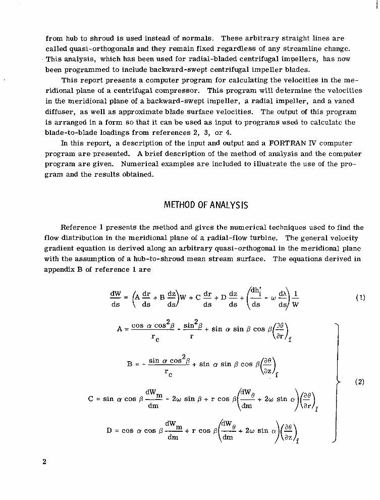
Figure 2. - Component of relative velocity Wn normal to arbitrary quasi*rthogonal.

Figure 1. - Coordinate system and velocity components.

The coordinate system and nomenclature a r e shown in figures 1 and 2. In this analysis, the total enthalpy at the inlet h i and the prerotation at the inlet X,

riVei, a r e assumed constant. Therefore, equation (1) reduces to

- = A - + B - W + C @ + D - dw ( :z dz) ds

dz ds d s d s

(14

Continuity must also be satisfied from hub to tip. The calculated mass flow across any fixed line from hub to tip must equal the specified mass flow. The mass flow is computed from

w = N a S pWnr A 0 ds

integrating from hub to tip along a quasi-orthogonal. The density is calculated from the isentropic flow equation with a correction for loss

in total relative pressure. This equation is derived in reference 1. The density equation is

3

where

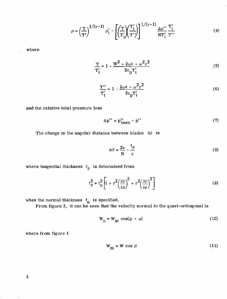
T W + 2 w X - w r - = 1 - 2 2 2

Ti -

2c T' P i

T; 2c T' P i

and the relative total pressure loss

Apt' = pysen - p"

The change in the angular distance between blades A0 is

where tangential thickness tg is determined from

when the normal thickness tn is specified. From figure 2, it can be seen that the velocity normal to the quasi-orthogonal is

wn = wm cos(* - CY)

where from figure 1

wm = w cos p

4

The flow angle p is determined from the mean stream surface, 8 = O(m), for each streamline, between the blades. Therefore,

where (de/dm), is the directional derivative along a streamline.

and (ae/ar), in equations (la) and (12) refer to the mean stream surface between the blades. The mean stream surface is assumed to deviate from the mean blade shape at a radius rb for a centrifugal machine. An approximate equation for determining rb is given by reference 5,

The ae/az and ae/ar in equation (9) refer to the mean blade shape. The (aO/az),

rb = ri e -0. AB)

The equation for the mean stream surface when r 2 rb is

1

rb

The boundary conditions used to obtain equation (14) were Po, the outlet flow angle; ob, the angular coordinate of the mean blade shape at rb; and (de/dm)b. Differentiating equation (14), we obtain

It will be noted that equation (la) is in terms of (M/az), and (i38/ar)f and that, on the mean stream surface, 8 is a function of the meridional distance m, for each streamline. The relation between them is

(E)f = sin a + (E)f cos a

5

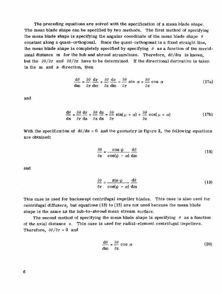
.The preceding equations are solved with the specification of a mean blade shape. The mean blade shape can be specified by two methods. The first method of specifying the mean blade shape is specifying the angular coordinate of the mean blade shape 6 constant along a quasi-orthogonal. Since the quasi-orthogonal is a fixed straight line, the mean blade shape is completely specified by specifying 8 as a function of the meridional distance m for the hub and shroud streamlines. Therefore, de/dm i s known, but the N/ar and ae/az have to be determined. If the directional derivative is taken in the m and s direction, then

and

de - ae d r ae dz ”” + - - = E s i n cy+-cos ae cy dm ar dm az dm ar az

With the specification of are obtained:

and

dO/ds = 0 and the geometry in figure 3, the following equations

” ae - cos @ dB az COS(@ - CY) dm

-

” ae - sin @ de ar cos(@ - 0) dm

-

This case is used for backswept centrifugal impeller blades. This case is also used for centrifugal diffusers, but equations (13) to (15) a r e not used because the mean blade shape is the same as the hub-to-shroud mean stream surface.

The second method of specifying the mean blade shape is specifying 8 as a function of the axial distance z. This case is used for radial-element centrifugal impellers. Therefore, 8 /ar = 0 and

”- de - ae cos cy dm az

6

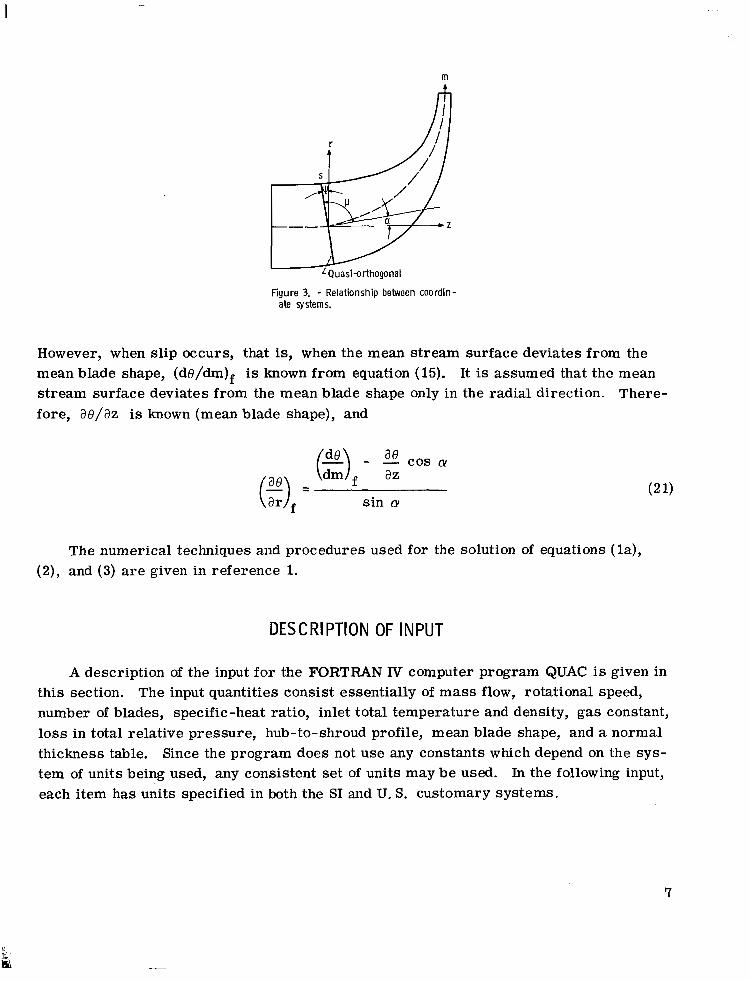
m

:Quasi"thogonal

Figure 3. - Relationship between coordinate systems.

However, when slip occurs, that is, when the mean stream surface deviates from the mean blade shape, (de/dm)f is known from equation (15). It is assumed that the mean stream surface deviates from the mean blade shape only in the radial direction. There- fore, ae/az is known (mean blade shape), and

- az = sin a,

cos a,

The numerical techniques and procedures used for the solution of equations (la), (2), and (3) a r e given in reference 1.

DESCRIPTION OF INPUT

A description of the input for the FORTRAN IV computer program QUAC i s given in this section. The input quantities consist essentially of mass flow, rotational speed, number of blades, specific-heat ratio, inlet total temperature and density, gas constant, loss in total relative pressure, hub-to-shroud profile, mean blade shape, and a normal thickness table. Since the program does not use any constants which depend on the system of units being used, any consistent set of units may be used. In the following input, each item has units specified in both the SI and U. S. customary systems.

7

The input format is shown in table I. The first card is a title card and this card must be put in. The input variables are *

Mx

KMX

MR

MZ

W

WT

XN

GAM

AR

TYPE

MT

SRW

MXBL

TEMP

ALM

RHO

PLOSS

number of quasi-orthogonals

number of streamlines

number of r-values of TN in the thickness table

number of z-values of TN in the thickness table

rotational speed, rad/sec

mass flow, kg/sec; slugs/sec

number of full blades

specific-heat ratio '

gas constant, J/(kg)(K); (ft)(lbf)/(slug)(OR)

integer; used as a code to indicate how arrays WA, Z, R, and DN a re given initially; the integer values a r e

0 These quantities will be calculated by the program.

1 Quantities just computed for previous case will be used for next case. (Used only when more than one case is calculated on single computer run. )

number of z-coordinates in ZT array

integer that will cause the program to print out certain values; used for debugging purposes; the integer values are

0 value when not debugging; usual case

13 SPLINE

16 SPLINT

21 RUUT

quasi-orthogonal number where blade starts

inlet total temperature, T;, K; OR

inlet prerotation, x, m /sec; ft /sec

inlet total density, pi , kg/m 3 ; slugs/ft3

loss in relative total pressure, Ap", N/m ; lb/ft

2 2

2 2

8

ANGR streamline rotation angle, deg (The streamlines are rotated so that the slope of the program's cubic spline curve i s not too large. G o d results are obtained from the cubic spline if the absolute value of the slope i s not greater than 1. Recommended angles are as follows: for animpeller, 45'; for a diffuser, 90'; and for an axial-flow compressor, 0'. )

KSTH determines the number of times the streamlines are smoothed-for each iteration (For example, if KSTH = 0, no smoothing occurs. This is the usual case (KSTH = 0). )

NPRT output control that determines which streamlines are printed out (For example, if NPRT = 1, every streamline is printed out; and if NPRT = 5, every fifth streamline is printed out. )

ITER number of iterations to be performed after ERROR is less than TOLER or after ERROR has started to increase (If ITER = 0, data will be printed for every iteration; if ITER > 0, data will be printed only for the final iteration. Normally ITER = 1, but for a first-run set ITER = 0 and check the first few iterations to see if the data were put in properly. )

K D determines compressor type (For a backward-swept impeller, KD = 0; for a diffuser and an axial-flow compressor, KD = 1; for a radial element impeller, KD = 2. )

SFACT blade multiplier to allow for splitter blades (For the case with no splitters, SFACT = 1.0; and for the case with splitters, SFACT = 2.0. )

ZSPLIT z-coordinate where splitter blade begins, m; f t (If there are no splitters, ZSPLIT > ZH(MX). )

BET0 outlet flow angle, Po, deg

CORFAC ratio of streamline correction used to calculated streamline correction (CORFAC affects the stability of the solution. If too large a value i s used, the new streamlines are less smooth than the previous ones. If a computa- tion is based on this set of streamlines, the calculated streamline correction becomes erratic. Therefore, it is important that the streamline correction used give a smooth streamline for the next iteration. A value of 0.1 i s recommended. )

SSN last quasi-orthogonal where smoothing is desired (For no smoothing,

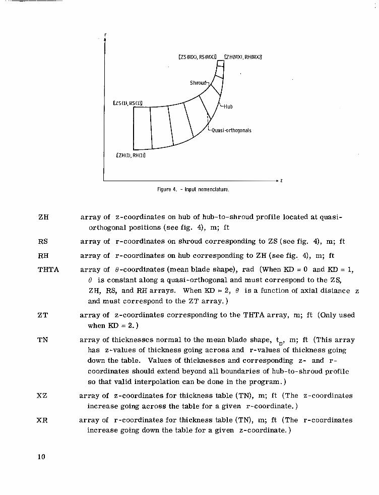
zs ar ray of z-coordinates on shroud of hub-to-shroud profile located at quasi-

SSN = 0. )

orthogonal positions (see fig. 4), m; f t

9

CZH(1). RH(1)I

I * z Figure 4. - Input nomenclature.

ZH ar ray of z-coordinates on hub of hub-to-shroud profile located at quasi- orthogonal positions (see fig. 4), m; ft

RS array of r-coordinates on shroud corresponding to ZS (see fig. 4), m; f t

RH ar ray of r-coordinates on hub corresponding to ZH (see fig. 4), m; f t

THTA ar ray of e-coordinates (mean blade shape), rad (When KD = 0 and KD = 1, 8 is constant along a quasi-orthogonal and must correspond to the ZS, ZH, RS, and RH arrays. When KD = 2, 8 i s a function of axial distance z

and must correspond to the ZT array. )

ZT ar ray of z-coordinates corresponding to the THTA array, m; ft (Only used when KD = 2. )

TN array of thicknesses normal to the mean blade shape, tn, m; ft (This array has z-values of thickness going across and r-values of thickness going down the table. Values of thiclmesses and corresponding z- and r- coordinates should extend beyond all boundaries of hub-to-shroud profile so that valid interpolation can be done in the program. )

xz ar ray of z-coordinates for thickness table (TN), m; f t (The z-coordinates increase going across the table for a given r-coordinate. )

XR array of r-coordinates for thickness table (TN), m; f t (The r-coordinates increase going down the table for a given z-coordinate. )

10

INSTRUCTIONS FOR PREPARING INPUT

Theta Constant Along a Quasi-Orthogonal

After the hub-to-shroud profile has been specified (fig. 5), the mean blade shape i s determined. The angular coordinate of the mean blade shape 8 is specified as a function of the meridional distance m for the hub and the shroud, as shown in figure 6. Values of 8 that are spaced to give good results from a cubic spline used in the program a r e selected. For a given value of 8, the meridional distances are determined for the hub and shroud from figure 6. These meridional distances are then converted to the

r A

- 2

Figure 5. - Hub-to-shroud profile. m S mh

Figure 6. - Hub and shroud mean blade shape. 0 = Oh).

proper z- and r-coordinates. Therefore, the z- and r-coordinates for the end points of a quasi-orthogonal have been determined. These are the quantities 8, rs, zs, rh, and Zh that are put in the program. The maximum number of quasi-orthogonal al- lowed is 21.

Theta Not Constant Along a Quasi-Orthogonal

This case is used for a radial impeller. The quasi-orthogonals are arbitrarily selected on the hub-to-shroud profile. They should be selected so that the program's

11

cubic spline curve wil l fit them smoothly. The mean blade shape is determined by specifying 0 as a function of the axial distance z, as shown in the third numerical example (p. 18). MT is the number of 0 -values used. It should, also, be noted that KD = 2 for this case.

Smoothing of Streamlines

If the streamlines are not smooth, a smoothing routine can be used. KSTH i s the number of times the streamlines are smoothed, and SSN is the last quasi-orthogonal where smoothing occurs. For an impeller, the streamline smoothing can take place only in the area shown in figure 7. It cannot take place in the other region because of the methods used. A recommended value for KSTH for smoothing i s 4.

r

n

I - - 2

Figure 7. - Streamline smoothing region for centrifugal impeller.

Another method of smoothing the streamlines is to put quasi-orthogonals upstream of the impeller. The mean blade shape i s extended into this region with the requirement of a negligible blade loading. These upstream quasi-orthogonals will allow a smoother transition into the impeller. For this case, MXBL is set equal to the quasi-orthogonal number where the blade starts. The first numerical example (p. 14) uses both these techniques.

12

DES CRI PTlON OF OUTPUT

An example of the output from the program is shown in table lI. This output is in U. S. customary units. Each section of the output has been numbered to correspond to the following description:

(1) The first output of the program is the input. (2) Output 2 gives the stagnation speed of sound at the inlet in meters per second

(ft/sec); the radius at which the mean stream surface deviates from the mean blade shape (FU3) in meters (ft); and a list of the number of iterations required to obtain a solution with the corresponding maximum streamline change in meters (ft).

(3) Output 3 gives some of the important quantities used in the calculation procedure which are also useful for debugging purposes. This output is given for every streamline printed out. Streamline 1 is at the hub and streamline 21 is at the shroud. The number of streamlines printed out is controlled by the input parameter NPRT. Items listed are

ALPHA

.RC

SM

BETA

TT

SA

SB

sc SD

angle between meridional streamline and z-axis, deg

curvature of meridional streamline, m-'; f t -

meridional distance, m; f t

flow angle, p, deg

tangential blade thickness, m; f t

1

A, eq. (2)

c, eq. (2)

B, eq. (2)

D, eq. (2)

(4) Output 4 gives the velocities and pressure for every streamline printed out. Items listed are

Z

R

WA

PRESS

WTR

WL

TTREL

z-coordinate, m; f t

r-coordinate, m; f t

relative velocity on mean stream surface, m/sec; ft/sec

static pressure, N/m2; -lb/ft2

suction-surface velocity, m/sec; ft/sec

pressure-surface velocity, m/sec; ft/sec

total relative temperature, K; OR

13

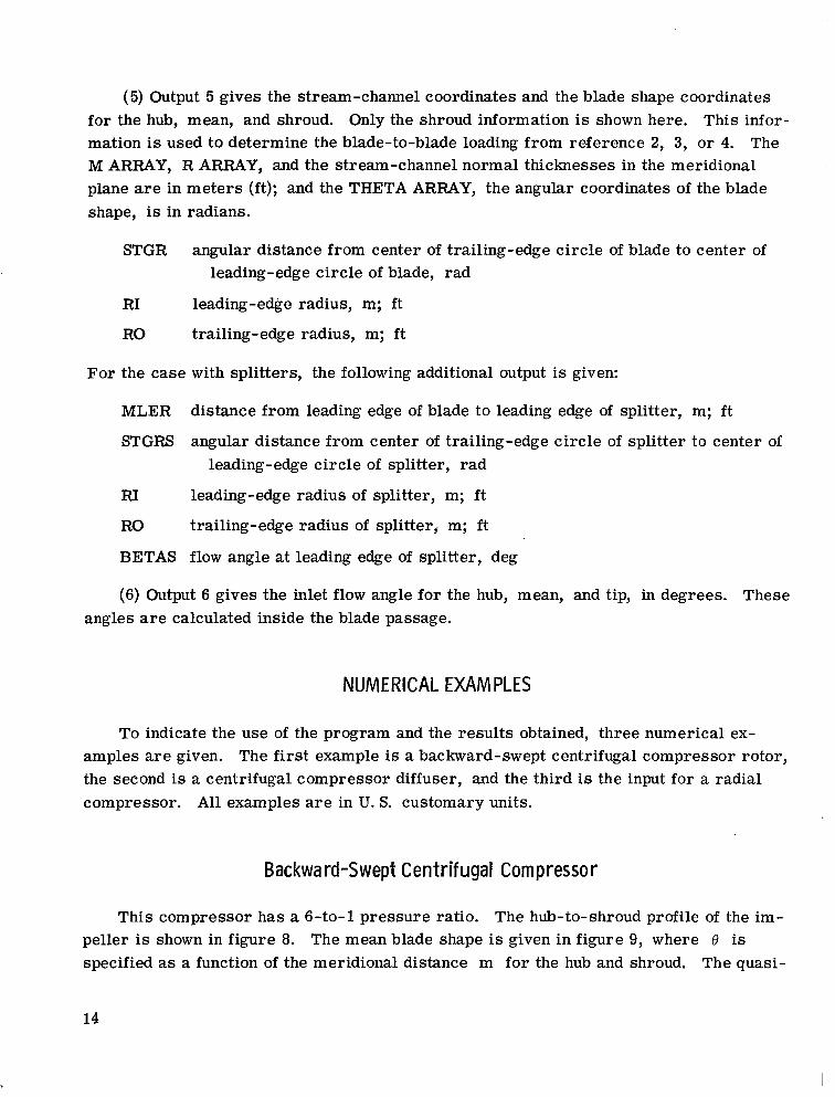
(5) Output 5 gives the stream-channel coordinates and the blade shape coordinates for the hub, mean, and shroud. Only the shroud information is shown here. This information is used to determine the blade-to-blade loading from reference 2, 3, or 4. The M ARRAY, R ARRAY, and the stream-channel normal thicknesses in the meridional plane are in meters (ft); and the THETA ARRAY, the angular coordinates of the blade shape, is in radians.

STGR angular distance from center of trailing-edge circle of blade to center of leading-edge circle of blade, rad

RI leading-edge radius, m; f t

RO trailing-edge radius, m; f t

For the case with splitters, the following additional output is given:

MLER distance from leading edge of blade to leading edge of splitter, m; f t

STGRS angular distance from center of trailing-edge circle of splitter to center of leading-edge circle of splitter, rad

RI leading-edge radius of splitter, m; f t

RO trailing-edge radius of splitter, m; f t

BETAS flow angle at leading edge of splitter, deg

(6) Output 6 gives the inlet flow angle for the hub, mean, and tip, in degrees. These angles are calculated inside the blade passage.

NUMERICAL EXAMPLES

To indicate the use of the program and the results obtained, three numerical examples are given. The first example is a backward-swept centrifugal compressor rotor, the second is a centrifugal compressor diffuser, and the third is the input for a radial compressor. All examples a r e in U. S. customary units.

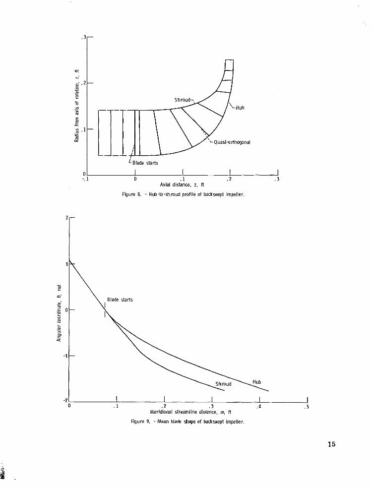
Backward-Swept Centrifugal Compressor

This compressor has a 6-to-1 pressure ratio. The hub-to-shroud profile of the impeller is shown in figure 8. The mean blade shape is given in figure 9, where 8 is specified as a function of the meridional distance m for the hub and shroud. The quasi-

14

Blade starts

1

1

U 2 rn- ai - m .c c U L 0 " 0 L m 3

4 c

-

-1

-2

-. 1 0 .1 .2 Axial distance, z, A

Figure 8. - Hub-to-shroud profile of backswept impeller.

3

I I I . 1 . 2 . 3 . 4 .5

Meridional streamline distance, m, ft

Figure 9. - Mean blade shape of backswept impeller.

15

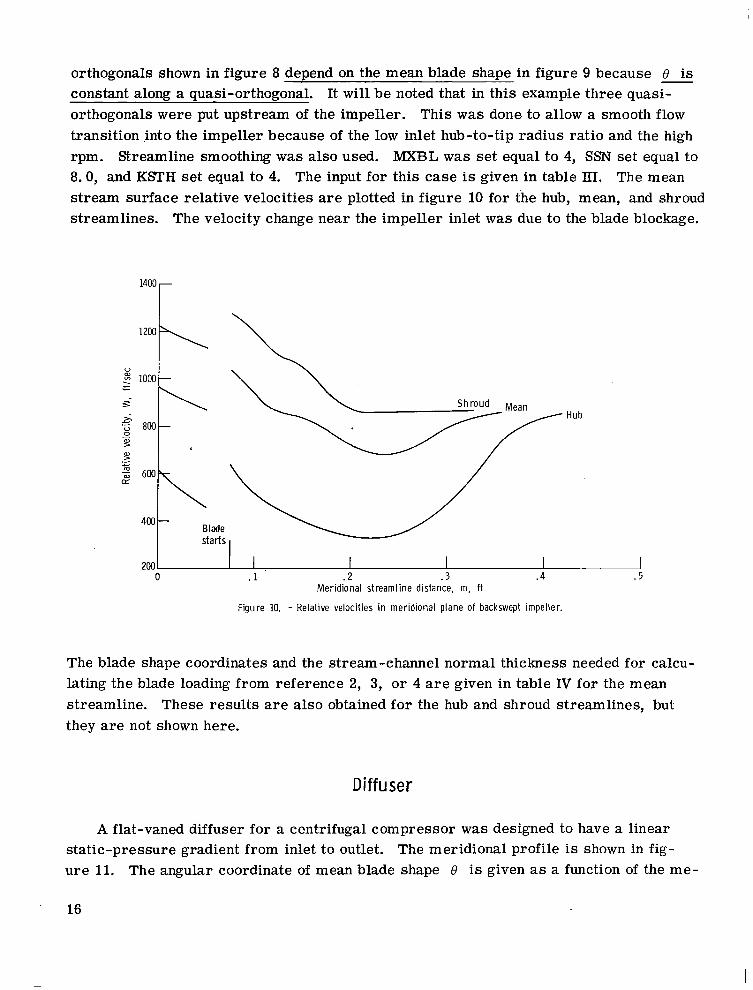
orthogonals shown in figure 8 depend on the mean blade shape in figure 9 because - e is constant along a quasi-orthogonal. It will be noted that in th i s example three quasi- orthogonals were put upstream of the impeller. This was done to allow a smooth flow transition into the impeller because of the low inlet hub-to-tip radius ratio and the high rpm. Streamline smoothing was also used. MXBL was set equal to 4, SSN set equal to 8.0, and KSTH set equal to 4. The input for this case is given in table III. The mean stream surface relative velocities are plotted in figure 10 for the hub, mean, and shroud streamlines. The velocity change near the impeller inlet was due to the blade blockage.

1200 1 4 L

400 - Blade starts

200. 0 . I . 2 . 3 . 4 . 5

Meridional streamline distance, m. ft

Figure 10. - Relative velocities in meridional plane of backswept impeller.

The blade shape coordinates and the stream-channel normal thickness needed for calculating the blade loading from reference 2, 3, o r 4 a r e given in table IV for the mean streamline. These results are also obtained for the hub and shroud streamlines, but they a re not shown here.

A flat-vaned diffuser for a centrifugal compressor was designed to have a linear static-pressure gradient from inlet to outlet. The meridional profile is shown in figure 11. The angular coordinate of mean blade shape 8 i s given as a function of the me-

16

I

dr thogona ls

- .Ol .02 .03 Axial distance. z, ft

Figure 11. - Hub-to-shroud profi le of compressor diffuser.

Meridional streamline distance, m, ft

Figure 12. - Mean blade shape for compressor diffuser.

17

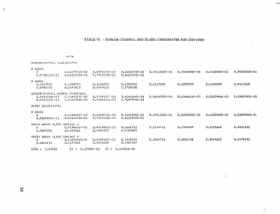
ridional distance m in figure 12. The quasi-orthogonals shown in figure 11 depend on the mean blade shape in figure 12 because 0 is constant along a quasi-orthogonal. The input for this case is given in table V. The mean stream surface velocities and the approximate blade surface velocities are plotted in figure 13 for the hub, mean, and shroud streamlines. The blade shape coordinates and the stream-channel normal thickness needed for calculating the blade loading from reference 2, 3, or 4 are given in table VI for the mean streamline.

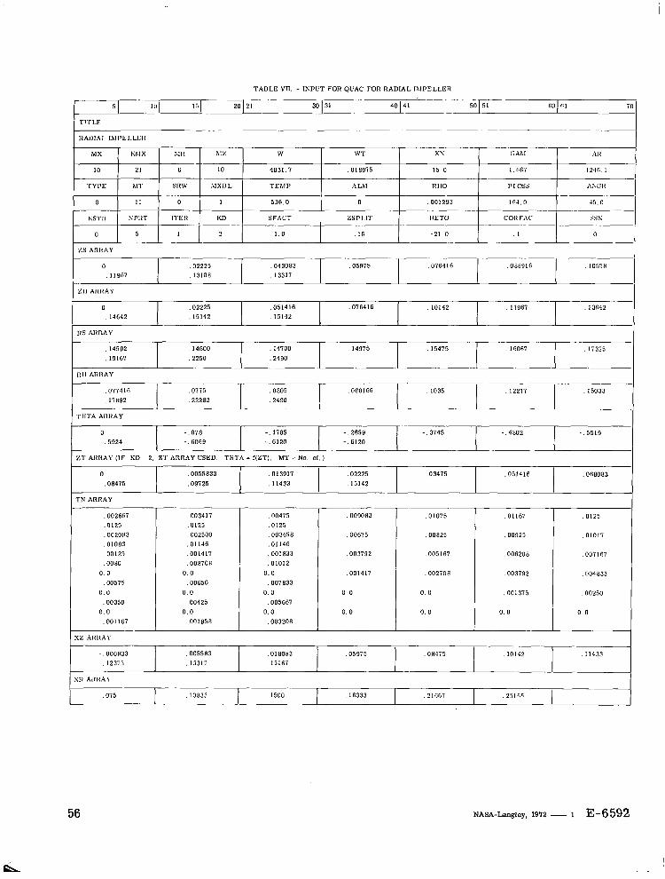
Radial Impeller

This example i s used to indicate the different input required. A hub-to-shroud profile is given in figure 14. The quasi-orthogonals for the profile shown are arbitrary and do not depend on the mean blade shape; that is, 0 is not constant along a quasi-

Suct ion surface

Mean stream surface

CI

\ Pressure surface

-2Wo .02 .M .06 .08 .10 Meridional streamline distance, m, R

Figure 13. - Blade loading diagram for hub and shroud of compressor diffuser.

I J .1 . 2

Figure 14. -

Axial distance, z, ft Hub-to-shmud profi le of radial impeller.

18

Axial distance, z, ft

Figure 15. - Mean blade shape for radial impeller.

orthogonal. The mean blade shape is put in as a function of the axial distance z, as shown in figure 15. Sample input is shown in table VII. The output obtained is the same as in the other examples.

PROGRAM DESCRIPTION

Main Program QUAC

The main program QUAC contains all the equations given in the method of analysis and makes the majority of the calculations. It will be noted that K i s used for the streamline number and I i s used for the quasi-orthogonal number. QUAC calls the subroutines RUUT, SMOOTH, INTGRL, CONTIN, SPLDER, SPLINE, LININT, and SPLINT to perform various functions such as smoothing, finding roots, integration, interpolation, and use of a cubic spline curve to determine derivatives. These subroutines, excluding RUUT and SMOOTH, are described in reference 1. A brief description of each is given herein.

The program variables for QUAC a r e

A temporary storage

AB temporary storage

19

AC

AD

AE

AL

ALM

AMLER

ANGR

AR

B

BA

BETA

BETAD

BETAS

BETAT

BETOH

BETOM

BETOT

C

CAL

CBETA

cr CORFAC

COSBD

COSBT

CP

C URV

DELBTA

DELTA

temporary storage

temporary storage

meridional length from leading edge

CY

see input

MLER (see output)

see input

see input

temporary storage

total weight flow between hub and Kth streamline

P

4

4 see output

exit blade angle at hub

exit blade angle at mean

exit blade angle at tip

temporary storage

cos a

cos p stagnation speed of sound a t inlet

see input

cos Pl cos P,

l/rc

Pt - PI

C P

calculated streamline correction

20

DENSTY

DN

DRDM

DTDMB

DTDMS

DTDR

DTDZ

DWMDM

DWTDM

E

ERROR

ERROR1

EXPON

G

GAM

HR

HZ

I

IND

INF

ITER

K

KD

KMX

KMXMl

KSTH

MR

MT

MX

P

distance along quasi-orthogonal from hub

- ( r w + W sin P)r A6 d dm

(de/W,,

ae/ar ae/az

de/dm at splitter leading edge

dWm/dm

dWe/dm

temporary storage

maximum calculated streamline correction for present iteration

ERROR from previous iteration

M Y - 1) temporary storage

Y

increment along quasi-orthogonal in r-direction

increment along quasi-orthogonal in z-direction

subscript to indicate number of quasi-orthogonal

code number for use by subroutine CONTIN

set equal to 1, when (ZH - ZS) = 0

see output

subscript used to indicate streamline number

see input

see input

KMX - 1

see input

see input

see input

see input

21

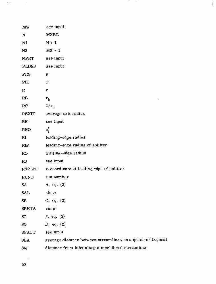
MZ

N

N1

N2

NPRT

PLOSS

PRS

PSI

R

RB

RC

REXIT

RH

RHO

RI

RIS

RO

RS

RSPLIT

RUN0

SA

SAL

SB

SBETA

sc SD

SFACT

SLA

SM

see input

MXBL

N + l

M x - 1

see input

see input

P

+ r

'b

l/rc average exit radius

see input

Pf

leading-edge radius

leading-edge radius of splitter

trailing-edge radius

see input

r-coordinate at leading edge of splitter

run number

A, eq. (2)

sin a

c, eq. (2)

sin P

P, eq. (2)

D, eq. (2)

see input

average distance between streamlines on a quasi-orthogonal

distance from inlet along a meridional streamline

SM1

sM2

SMF

SMEXIT

SMRB

SRW

SSN

STGR

T

TANBB

TANS

TEMP

THTAF3

THTAF

THTAS

THH

TNHC

THHl

THH2

THM

THMC

THMl

THM2

THS

THSC

T HSI

THS2

meridional distance from first quasi-orthogonal to quasi-orthogonal that is before point where stream surface deviates from blade surface

meridional distance from first quasi-orthogonal to a quasi-orthogonal that is after point where stream surface deviates from blade surface

fractional meridional distance

meridional distance from first quasi-orthogonal to trailing edge of blade

meridional distance from first quasi-orthogonal to point where mean stream surface deviates from mean blade shape

see input

see input

see output

tn (interpolated value)

tan 43 tan ps, at leading edge of splitter

T;

Of

OS

'b

mean blade shape 8-coordinate at hub

temporary storage

blade shape, 8-coordinate a t hub on surface 1

8-coordinate at hub on blade surface 2

8-coordinate of mean blade shape at mean

temporary storage

8-coordinate at mean on blade surface 1

8-coordinate at mean on blade surface 2

8-coordinate of mean blade shape at shroud

temporary storage

8-coordinate at shroud on blade surface 1

8-coordinate at shroud on blade surface 2

23

f

TN

TOLER

TSPLIT

T P P l P

TTREL

TT

TYPE

T1P

W

WA

WAS

WASS

WT

WTFL

WTHRU

WTR

WL

XN

XR

xz YA

YH

YM

YS

Z

Z EXIT

ZH

zs Z SPLIT

ZT

see input

iteration tolerance

normal blade thickness at leading edge of splitter

T"/T;

see output

see input

T/T;

w

W

W*, eq. (13) of ref. 1

W**, eq. (13) of ref. 1

total mass flow

calculated total mass between hub and K streamline th

wn Wt, eq. (10) of ref. 1 (suction-surface velocity)

pressure-surface velocity

see input

see input

see input

average weight flow per unit length crossing a quasi-orthogonal

temporary storage

temporary storage

temporary storage

Z

average z-coordinate at exit

see input

see input

see input

see input

24

Subroutine RUUT

Subroutine RUUT finds the root between two given points. It is used to find the meridional distance where the mean stream surface deviates from the mean blade shape when the radius at which this occurs is given. If the root cannot.be found within the tolerance, a message is printed out and the input arguments are listed. If-there is trouble in finding a root, set SRW = 21 in the input and all the input to the subroutine wi l l be printed out.

The calling sequence for RUUT is

CALL RUUT(SM1, SM2, RB, SMRB, SM( 1, K), R( 1, K), MX)

meridional distance of quasi-orthogonal before point desired (input)

meridional distance of quasi-orthogonal after point desired (input)

radius at point desired (input)

desired meridional distance (output)

array of m-coordinates (input)

array of r-coordinates (input)

number of r-coordinates (input)

Subroutine SMOOTH

Subroutine SMOOTH smoothes the streamlines to obtain a better numerical solution. It uses the hub streamline as the base streamline for the smoothing operation.

The slopes of the quasi-orthogonals a r e

ysI - yhI m, =

xsI - XhI

and the streamline slopes are

YI+1 - YI-1

xI+l - 1 ?.( = (2 3)

25

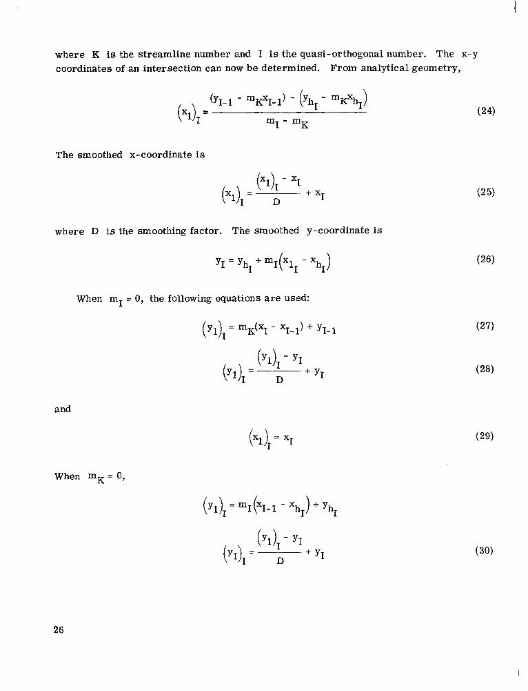
where K is the streamline number and I is the quasi-orthogonal number. The x-y coordinates of an intersection can now be determined. From analytical geometry,

The smoothed x-coordinate is

where D is the smoothing factor. The smoothed y-coordinate is

and

y I = y hI + m I( x l1 - XhI)

=

When mK = 0,

26

t

and

The value of D is 2 for all quasi-orthogonals except for the last-three, where smoothing occurs. The values of D for these three are 2.6667, 4.0, and 8 . 0 , respec- tively. This w a s done so that there would not be any discontinuities when only certain sections of the streamlines are smoothed.

The calling sequence for SMOOTH is

CALL SMOOTH(Z( 1, K), R( 1, K), ZH, RH, A B , SSN, INF)

where

z( 1, K) z-coordinate of streamline

R( 1, K) r-coordinate of streamline

ZH z-coordinate of hub streamline

RH r-coordinate of hub streamline

AB slope of quasi-orthogonals, mI

SSN last quasi-orthogonal where smoothing is desired

INF indicator for quasi-orthogonals with a slope of infinity

The program variables are

D

SLOPE

SLOPE 1

X

XH

x 1

Y

YH

Y1

smoothing factor

slope of quasi-orthogonals, mI

streamline slope, mK

z-coordinate of streamlines

z-coordinate of hub streamline

z-coordinate of smoothed streamline

r-coordinate of streamlines

r-coordinate of hub streamline

r-coordinate of smoothed streamline

27

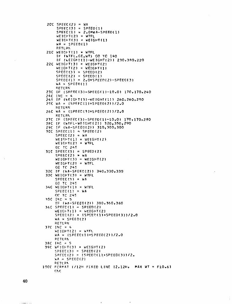
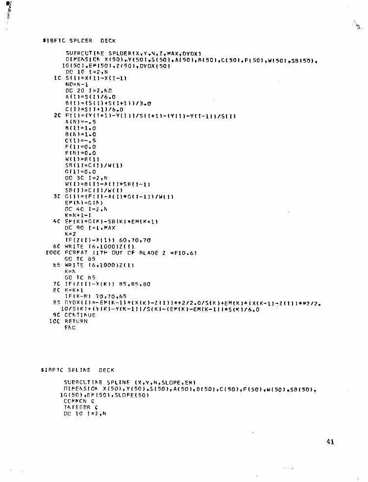
Other Subroutines

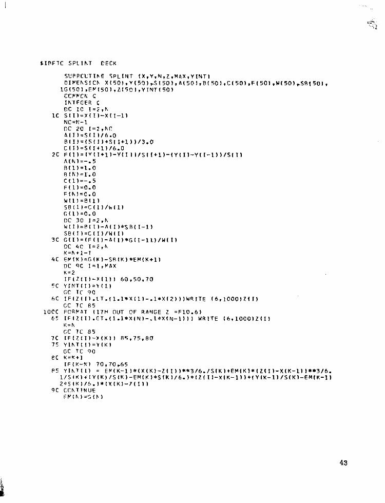
Subroutines INTGRL, CONTIN, SPLDER, SPLINE, LININT, and SPLINT are described in reference l. INTGRL is used for numerical integration. CONTIN is used to determine the hub velocity for the next continuity iteration. SPLDER is used to determine the values of the derivatives at the specified interpolated points. SPLINE is used to determine the first and second derivatives. If there is a problem with the SPLINE subroutine, set SRW = 13'in the input and the input and output of the SPLINE subroutine will be printed out. LININT is used to determine the interpolated values of the normal blade thickness from the given thickness table. SPLINT is used for interpolation. The input and output data for SPLINT will be printed out if SRW = 16.

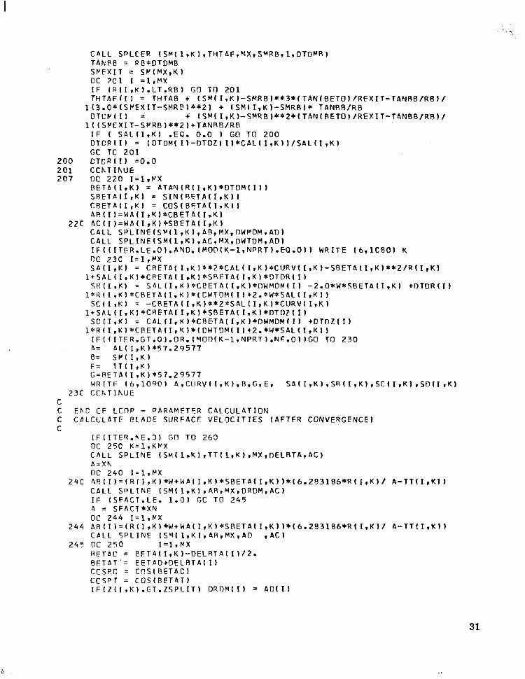
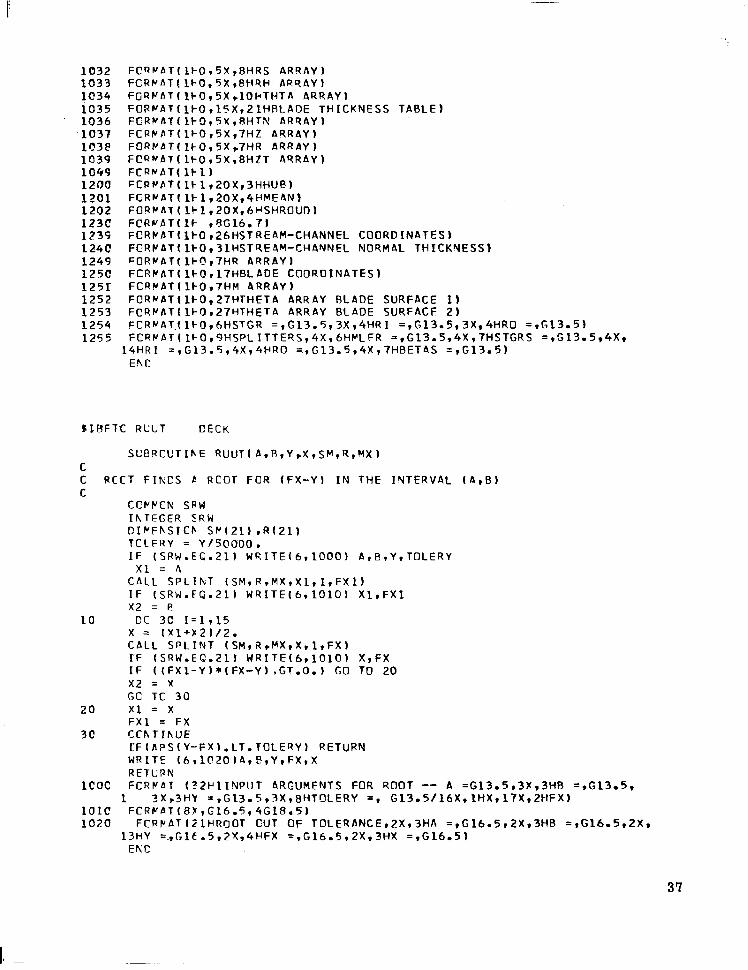
PROGRAM LISTING S I R F T C C L ' A C DECK

28

UTCLER = WT/100000. TCLER = (RS(l)-SH(1))/5000. IF(RS(l).EC.RH(L)) TOLER= (ZH(l)-ZS(1))/5000. DC 11C K = l r K M X

R4(1)=0. DC 120 K=ZrK?'X

1IC S t ' ( ' l r K ) = C .

12C B A ( K ) = FLCAT(K-l)*WT/FLOAT(KMX -1) nc 13C I = l T p X

13C Ch! ( I 1-1 ) = C A h G R = AhGRf57.29577

145 CChTIhUE CI = SQRT(CAM*AR*TEMP) WRITE(6r1049) WRITE (6910501 CI

29

I

b

31

L C EhC nF @LADE SURFACE VELOCITY CALCULATIONS C S T A R T CALCULATION OF WEIGHT FLOW V S o DISTANCE FROM HUB

L C E h r C F L C L l P - WEIGHT FLnW CALCUL4TION C CcLf.CLnTF: STREAMLINE COORDINATES FOR NEXT ITERATION

32

I‘

1 0 3 2 1 0 3 3 1 0 3 4 1 0 3 5

’ 1 0 3 6 1 0 3 7 I Q 3 P 1 0 3 9 1 O W 1 2 0 0 1 3 0 1 1 2 0 2 1 2 3 C 1 2 3 9 1 2 4 C 1 2 4 9 1 2 5 c

1 2 5 2 1 2 5 3 1 2 5 4 1 2 5 5

1 2 5 1

F C Q w d T f 1 F O p 5 X ~ R H R S A R R A Y 1 F C R t ’ d T ( l b O * S X t P H 4 H A P S A Y ) F G Q C A T ( l F O * S X , l O ~ T H T A A R R A Y ) F O R Y A T ( l F O * l S X ~ Z l H R L A D E T H I C K N E S S T A B L E ) FCRPATI lF !3 r5Y*RHTh! A R f 7 A Y ) F C R P b T ( l F O * 5 X * 7 H Z A R R A Y ) F O R C l T l l k 0 * 5 X + 7 H R A R R A Y 1 F C Q w A T t l F 0 9 5 X 9 8 H Z T A r l R A Y F C R p b T ( 1 F l ) F C P ~ b T ( 1 ~ 1 , 2 0 X , 3 H H U e ) F C R ~ b T ( l F l r 2 0 X 1 4 H M E n N ) FOQYAT I l+ 1 * 2 0 X * 6wSHROUD 1 FCRk’bT( lk r S G l 6 . 7 1 FCRCbT11FOt26HSTREAM-CHANNEL COORDINATES) F C R C ~ T ( ~ ~ O I ~ ~ H S T ~ E ~ ~ - ~ H A ~ N E ~ NORMAL THICKVESS) F O R V A T ( l b Q 9 7 H R A R R A Y 1 F C R C ~ T ( ~ F O I ~ ~ H B L A D E COORDINATES) F C R V A T ( l F O * ? H M 4 R R A Y I F O R w A T ( l b 0 * 2 7 H T H E T A A R R A Y BLADE SURFACE 1) F C R P b T ( l b 0 * 2 7 H T H E T A A R R A Y BLADE SURFACE 2 ) FCRwAT. f lFO*hHSTGR = rG13 .5 ,3Xv4HRI = rG l3 .5 *3X*4HRO = rG13 .5 ) F C R t ’ b T ( 1 ~ 0 * 9 H S P L I T T E ~ S ~ 4 X * 6 H ~ L ~ R = * G 1 3 . 5 * 4 X * 7 H S T G R S = ~ G 1 3 . 5 ~ 4 X *

Eh I l 1 4 H R I = * G 1 3 . 5 , 4 X ~ 4 H R O = r G 1 3 . 5 * 4 X * 7 H B E T 4 S = * G 1 3 . 5 )

S l B F l C R U L T C E C K

S U B R C C T I h E R U U T ( A * ~ I Y ~ X * S M , S * M X ) C C RCCT FIKCS C R C O T FGR ( F X - Y ) IN THE INTERVAL (AvB)

CCCCCN SPW I h T F G E R C R W D I C F h S I C h S P ’ ( 2 1 ) 1 R ( 2 1 ) TCLERY = Y / 5 @ 0 0 0 . I F ( S R W . E C . 2 1 ) W Q I T E ( 6 * 1 0 0 0 ) A r B , Y v T O L E R Y

X 1 = A CALL SPLIhT ( S M g R * M X * X l V l * F X l ) I F ISRW.FG.21) W 9 I T E 1 6 ~ 1 0 1 0 1 X l r F X l x 2 = i?

x = ( X l + > 2 ) / 2 . C b L L S P L I N T ( S M * R , M X t X * l r F X ) I F (SRW.EC.211 W R I T E ( 6 * 1 0 1 0 ) X * F X I F ( ( F X l - Y ) * ( F X - Y ) , G T . O . ) GO TO 20 x 2 = x GC T C 30

2 0 x 1 = x F X l = FX

3 c C C h T I h U E I F ( A P S ( Y - F X ) . L T . T O L E 4 Y ) RETURN W R I T E ( 6 * 1 @ 2 O ) A r P r Y * F X * X R E T L P K

L O C C 3C I = l r 1 5

l C O C FCRPAT ( 3 2 P l I N P U T 4RGUMFNTS FOR ROOT A =G13 .5*3X*3HB = rG13 .5* 1 3Xp3HY =rG13.5*3X*8HTQLERY = * G 1 3 o 5 / 1 6 X * l H X * 1 7 X * 2 H F X )

l O l C F C R C 4 T ( 8 r , G 1 6 . 5 * 4 G l R . 5 1 1020 FCRCbT121HROOT CUT OF T O L E R A N C E * 2 X * 3 H A = * G 1 6 0 5 r 2 X * 3 H B = r G 1 6 . 5 * 2 X *

1 3 H Y = . ~ G l C - 5 * 2 Y * 4 H F X = * G 1 6 . 5 r Z X * ? H X = ~ G l 6 . 5 ) E K C

37

SIBFTC S C C C T H DECK

C C 5

C C 6

1 0

20

S I e F T C IhTGRL D E C K

38

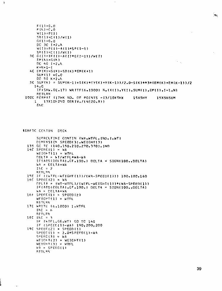
8LRF’ IC C C h T I N C E C K

39

2CC S P E E C ( 2 ) = WA S P E E C ( 3 ) = S P E E D I I )

W E I C P T ( 2 ) = WTFL W E I G F T ( 3 ) = W E I G P T ( 1 ) WA = S P E E G ( 1 ) RETLRh

S P E E C I l ) = ZoO*WA-SPEED( 1)

2 f C WEICI-T ( 1 1 = WTFL I F ( kTFLoGEoWT) GO TO 140 I F ( k E I G ~ T ( l ) - W E I G H T ( 2 ) ) 23093909220

22C W E I G F T ( 3 ) = W E I G P T ( 2 ) W E I G k T ( 2 ) = W E I G P T ( 1 ) S P E E E ( 3 ) = S P E E D I 2 ) S P E E C I Z ) = S P E E O ( 1 ) S P E E C ( 1 ) = 2.O+SPEEf l (2) -SPEEC(3) kA = S P E E O I l ) RETURN

23C I F (SPFEC(31-SPEEC(L)-lOoO) 17091709240 24C I N C = 4

25C WA = ( Z P E € C ( l ) + S P E E D ( Z ) ) / 2 . 0 2 4 5 I F ( k E I G ~ T ( 3 ) - W E I G H T ( l ) ) 2 6 0 9 2 6 0 9 2 5 0

RETCRh

RETCRh 26C W A = ( S P E E C ( 3 ) + S P E E D ( 2 ) ) /2 .0

27C IF (SPEEC(3)-SPEED(l)-lO.O) 17011701280 ?@C IF ( h T F L - W E I G H T ( Z ) . ) 3 2 0 , 3 5 0 9 2 9 0 29C IF ( k A - S F E E D ( 2 ) ) 3 L 0 9 3 0 0 9 3 0 0 3 C C S P E E C ( 1 ) = S P E E D ( 2 )

SPEECC2) = W A k ' E I G H T ( 1 ) = WEIGHT(.?) W E I G P T ( 2 ) = WTFL GC TC 2 4 5

31C S P E E C ( 3 ) = S P E E D I Z ) S P E E C f 2 ) = W A W E I G P T ( 3 ) = W E I G H T ( 2 ) W E I G P T ( 2 ) = WTFL GO TC 2 4 5

32C I F ( W b - S F E F D ( 2 ) ) 34093309330 3 3 C W E I G P T ( 3 ) = WTFL

S P E E C t 3 ) = W A GO TC 2 4 :

3 4 C W E I G F T ( 1 1 = WTFL S P E E C ( 1 ) = WA GC TC 245

3 5 c IKC = 5

36C S P E E C ( 1 ) = S P E E D ( 2 ) I ' F ( h A - S F E E D ( 2 ) ) 38093609360

W E I G F T ( 1 ) = GJEIGFT(2)

HA = S P E E D ( ? ) RETURN

W E I G P T ( 2 ) = WTFL W A = ( S P E E C I 1 ) + S P E E D l 2 ) I l 2 . 0 RETCRR

S P E E C ( 2 ) = ( S P c E C ( l ) + S P E E D ( 3 ) ) / 2 0 0

37c I N C = 4

38C I h C = 5 39C h ' F I G F T ( 3 1 = W E I G H T ( 2 )

S P E E t ( 3 ) = SPEED121 S P E E C ( 2 ) = ( S P E E ~ ( l ) ~ + S P E E D 1 3 ) ) / 2 . k d = S P E E D ( 2 ) RETLRh

Ehr, l r jCC FCRWAT ( / 1 2 H F I X E D L I N E I 2 9 l Z H 9 M A X WT = F10.61

40

SLRF'IC SFLIkE DECK

4 1

Lewis Research Center, National Aeronautics and Space Administration,

Cleveland, Ohio, November 16, 1971, 132-15.

44

L

I

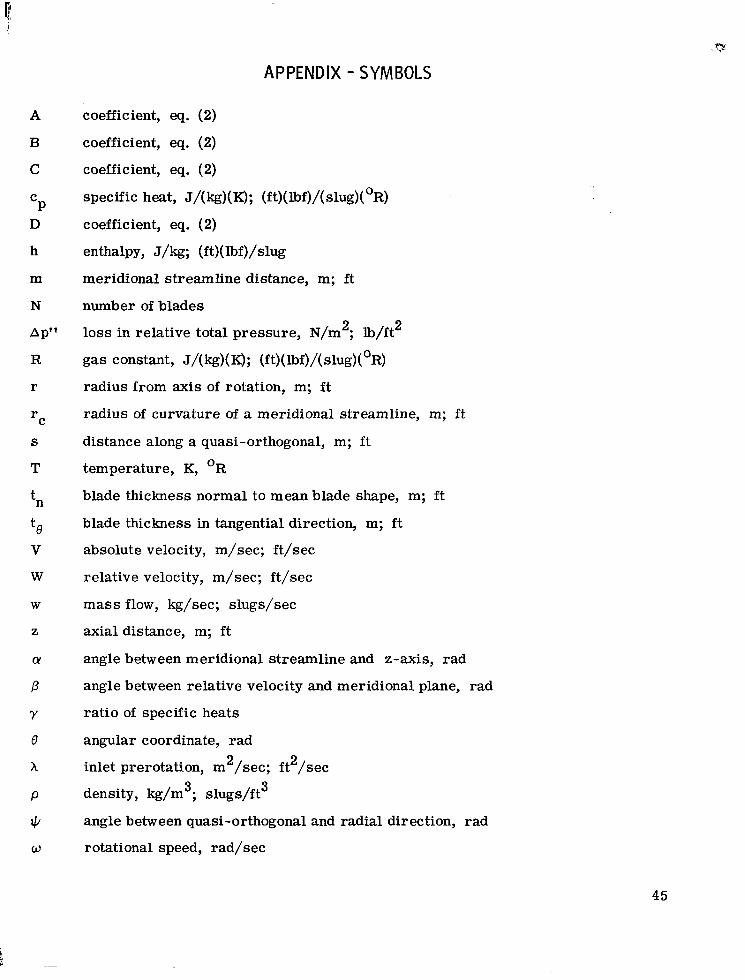
APPENDIX - SYMBOLS

A

B

C

C P D

h

m

N

Ap"

R

r

rC

S

T

tn

te V

W

W

z

CY

P Y

e x P

Q w

coefficient, eq. (2)



specific heat, J/(kg)(K); (ft)(lbf)/(slug)(OR)


enthalpy, J/kg; (ft)(lbf)/slug

meridional streamline distance, m; f t

number of blades

loss in relative total pressure, N/m2; lb/ft

gas constant, J/(kg)(K); (ft)(lbf)/(slug)(OR)

radius from axis of rotation, m; f t

radius of curvature of a meridional streamline, m; ft

distance along a quasi-orthogonal, m; ft

temperature, K, OR

blade thickness normal to mean blade shape, m; f t

blade thickness in tangential direction, m; f t

absolute velocity, m/sec; ft/sec

relative velocity, m/sec; ft/sec

mass flow, kg/sec; slugs/sec

axial distance, m; f t

angle between meridional streamline and z-axis, rad

angle between relative velocity and meridional plane, rad

ratio of specific heats

angular coordinate, rad

inlet prerotation, m /sec; f t /sec

density, kg/m3; slugs/ft 3

angle between quasi-orthogonal and radial direction, rad

rotational speed, rad/sec

2

2 2

45

I I I I , ..I ..,.,,.I I I I I .. .".1.1-.1.-..-.

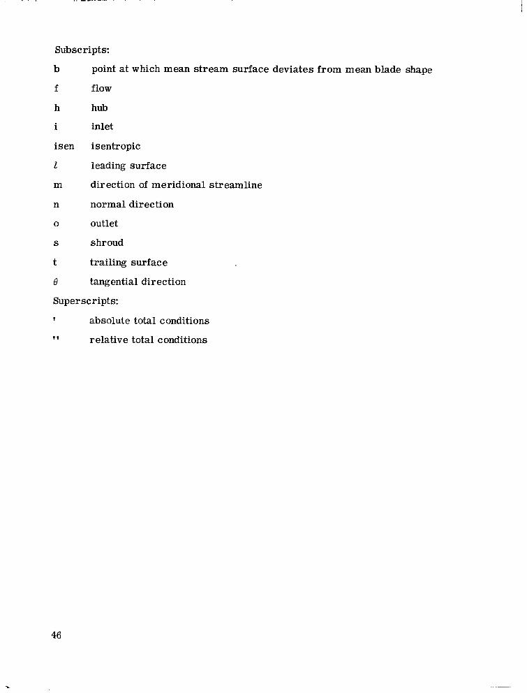
Subscripts:

b

f

h

i

isen

2

m

n

0

S

t

0

point at which mean stream surface deviates from mean blade shape

flow

hub

inlet

isentropic

leading surface

direction of meridional streamline

normal direction

outlet

shroud

trailing surface

tangential direction

Superscripts:

1 absolute total conditions

relative total conditions 1 1

46

REFERENCES

1. Katsanis, Theodore: Use of Arbitrary Quasi-Orthogonals For Calculating Flow Dis- tribution In the Meridional Plane Of A Turbomachine. NASA TN D-2546, 1964.

2. Katsanis, Theodore; and McNally, William D. : Fortran Program For Calculating Velocities And Streamlines On A Blade-To-Blade Stream Surface Of A Tandem Blade Turbomachine. NASA TN D-5044, 1969.

3. Katsanis, Theodore; and McNally, William D. : Revised Fortran Program For Cal- culating Velocities And Streamlines On A Blade-To-Blade Stream Surface Of A Turbomachine. NASA TM X-1764, 1969.

4. Katsanis, Theodore: Fortran Program For Calculating Transonic Velocities On A Blade-To-Blade Stream Surface Of A Turbomachine. NASA TN D-5427, 1969.

5. Stanitz, John D. ; and Prian, Vasily D. : A Rapid Approximate Method For Determin- ing Velocity Distribution On Impeller Blades Of Centrifugal Compressors. NACA TN 2421, 1951.

47

. . .. . . . . . ..- -

T A B L E 1. - INPUT FORM FOR QUAC

5 10 15 20 21 30 31 40141 50p"-"60)m r\H I TITLE

" _ _ _ ~ ~ ~ - ~ ~~ -

-___ ~ _ _ _ ~ _ _ ~ _ _ ~~~

MX ClAbl XN W T W M Z X1 R YblX

T Y P E A s t i l l PLOSS RHO A Lhl TEMP n l x n L SRW M T

KSTH SSK C O R F A C B E T 0 Z S P L I T S F A C T Kz) ITER NPRT

ZS ARRAY

% I 1 ARRAY

RS ARRAY

RH ARRAY

THTA ARRAY

Z T ARRAY (IF KD = 2. Z T ARRAY USED. THTA = I(ZT). M T = No. o f . )

I TN ARRAY

YZ ARRAY

<R ARRAY

t I

48

I ,...I I I I.

k

TABLE 11. - SAMPLE OUTPUT

I P P E L L E R 4 Y E S - 1 A 3 B

RUY h C . 1 I N P U T C A T A C A R D L I S T I N G

P) l ,KYX V G C Z W WT X N 13 21 5 6 7P53.9R 0.62160E-01 15-COO0

G A M 1.40POO 1716.20

AR

45.0000 AfJGR

8.00000 S S N

T Y P E Y T S R k Y X R L T F M P -a -0 -0 4 51~.7no

A L M -0

K S T k N P R T I T E P K O S F A C T 4 5 1 -0 2.00000 0.12500

Z S P L I T

Z S A R R b Y -0.7543CE-01 -0.50000E-01 -0.25OOOF-01 0.S7583E-01 0.13142 0.16958

ZH A R R b Y -0.75430E-31 -0.50000E-01 -0.25000E-01 C .I5575 0.18433 0.201co

R S 4 R R A Y C.14125 0.14692

0.14125 0.14125 0.15712 0.18291

C.42375E-01 0.42375E-01 0.42375E-01 R H A R P A Y

o.e5655~-01 0.12620 0.17845

T H T A A R R A \

- I . l00CC -1.30000 0.69770 1 .c8290

-1.50000 0.33800

B L d C E T F I C K N E S S T A R L E

TF: A R R A Y C.41670E-02 0.5OOOOE-02 0.58330E-02 Cm3125CE-02 0.37500E-02 0.43750E-02 0.2OR30E-02 0.20830E-02 0.22500E-02

-C -C

-0 -0

-0 -0

RPl r l 0.2377OE-02 1622.80

P L O S S

-53.9500 B E T 0

0.10000 C~IRFAC

0.9920AF-02 0.18892

0.39682E-01 0.19167

0 0.18258

0.72917E-01

0. L Z O P 3

0.14320

0.60442E-01

-0.90000

0.10167E-01 0.205n9

0 0.20475

0.54000E-01 0.20617

0.14125 0.20487

0.14125 0.22757

0.14135 0.25004

0.42375E-01 0.20711 0.22771

0.42375E-01 0.43229E-01 0.25004

0 - 1.60000

-0,125'70 -1.67500

-0.5000O -1.75000

0.58330E-02 0.75000E-02

0.33330E-02

-0 -0

0.7500OE-02 0.75000E-02 0.500OOE-02 0.20830E-02

-0

0.75000E-01 0.75000E-02 0.59330E-02 0.54170E-02 0.50000E-02

0.14170 0.18333 0.20833

0.4167CE-Q1 0.91580E-01 0.14125 R A R R A Y

0.20833 0.25417

STAG. S P E E C C F S O U N C

R R = C.21747 I T E R A T I C Y h 0 . 1 I T E R A T I C Y hO. 2

I T E R A T I C Y he. 4

I T E R b T I C Y h C . 6 I T E Q A T I C N hO. 5

I T E R A T I C N h C . 7 I T E R A T I C Y h O . 8 I T E Q b T I C ' I h C . 9 I T F R A T I C V h O . 10

I T E Q A T I C N hO. 12 I T E R A T I C V hl?. 13 I T E R A T I C U h 0 . 14

I T E R P T I C N hC. 16 I T E R b T I C Y h C . 1 5

I T E R A T I C Y h C . 17 I T E R A T I C Y h 0 . 18

I T F R A T I C N h C . 20 I T E R A T I C N hC. 19

ITERATICN nc. 3

ITERATICY nC. 1 1

A T I N L E T = 1116.36

C.018577 C.015987 C.014245 0.012898 C.011650 c.010522 C -009499 C.000590 0.007747 C. 006983 C.006293

C.005104 O.00Sh6R

0.004611 C.004148 C.003731 C.003354 0.003015 C.002709 C.002434

MA-X. S T R E A M L I N E C H A N G E = MAX. S T R E A M L I N E C H A N G E = MAX. S T R E A M L I N E C H A N G E = MAX. S T R E A M L I N E C H b N G E = MAX. S T R E A M L I N E C H A N G E = MAX. S T R G A M L I N E C H A N G E = MAX. S T S E A M L I N E C H A N C E = MAX. S T R E A M L I N E C H h N G E = MAX. S T R E A M L I N E C H A N C E = MAX. S T R E A M L I N E C H A N G E = MAX. S T R E A M L I N E C H A N G E = MAX. S T R E A M L I N E C H A N G E = M 4 X . S T R E A M L I N E C H A N G E = MAX. S T R E A M L I N E C H A N G E = MAX. S T R E A M L I N E C H A N G E = MAX. S T R E A M L I N E C H A N G E = MAX. S T R E A M L I N E C H A N G E =

MAX. S T R E A M L I N E C H A N G E = MAX. S T Q E A M L I N F C H A Y G E =

MAX. S T R E A M L I N E C H A Y G E =

49

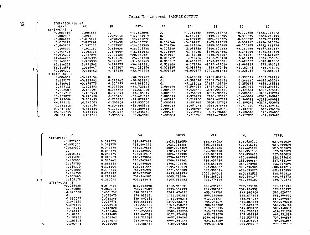
TABLE TI. - Continued. SAMPLE OUTPUT m 0

3

I T E R I T I C N hO. 67

S T R E b P C I h E 1 A L P P b

-0 ,001619

-C.006421; c.oozc22

-0.063958 0.C23697

26.741523 4.145020

44.955225 64.044206 79.5493,80

e 8 . 2 1 8 5 ~ e5.266557

3 T R E P Y L I K E 6 50.105220

3.004852 2.685177 1.986931 2.757111 4.062589 8.484717

17.853872 27.212C84 44.228121 71.731218 e1.412612 e5.929255 e8.307595

R C

0.001666

-0.015122 0.003332

-0.357136 0.057244

4.201212 7.103331 7.187098 5.886395 3.979333 2.981542 2.065947 0.938462

-0.147154 -0.289882 -0.676773

1.8022R3 2.746191 1.156943 5.723180 3.301493

10.548003 7.527054 4.883134 2.713154 1.207301

9 2 R E b P L I k E 1 2

-0.05COOO -0.075430

-0.025000 0. 0 -0 1C 167 C.354000 C.12C830 0.155750 0.184330 0.201000 0.204750 0.205890 0.20C170

-0.075430 -0.05COOO -0.025000

0. 0.01C065 0.047529

C.13C711 C.16t728 0.192875 C.19S133 C.201395

S T R E L Y L I N E 6

0.09e186

‘2.202443

SM

0. 0.025430 0.050430 0.075430 0.085597 0.129438 0.198449 0.241520 9.292126 0.345971 0.374875 0.395507 0.417838

0. 0.025462 0.050483

0.085582 0.075500

0.123293 0.175706 0.210372 0.253909 0.304334 0.331991 0.353242 0.375634

R

0.042375 0.042375 0.042375 0.042375 0.042375 0.043229 0.060442 0.085655 0.126200 0.178450

0.227710 0.207110

0.250040

0.079456 0.080727 0.081767 0.082675 0.083266

0.098518 0.087576

0.136486 0.112028

0.179603 0.206542 0.227673 0.250040

RETA

-33.192096 -32.066519

-28.558731 -30.721272

-26.058385 -16.202538

-20.260381 -16.851673

-31.632465 -25.751180

-41.230254 -36.617331

-53.949998

-50.771102

-48.883551 -50.012261

-46.720125 -44.589050 -37.185014 -32.627673 -29.878273 -29.933708 -33.680576 -36.389583

-53.949998 -40.335552

W A

611.987427 528.864166 453.919613 638.129807

440.273067 575.012436

335.542908 419.009806 521.131454 764.574997 810.338303 762.966583 923.105478

811.558098 748.752609 698.583702

830.890221 704.661819 631.463585 664.214363 666.233994 797.847511

767.949860 819.723518

924.466454

878.032661

TT

0 . 0. 0. 0.004744 0.004834 0.005290 0.006449 0.006957 0.006422 0.005817 0.006209 0.006235 0.005918

0. 0. 0. 0.004849 0.004847 0.004838 0.005029 0.005245 0.005329 0.00506P 0.005310 0.005248 0.005031

SA

-7.071380 -6.649137 -6.169999 -5.349131 -4.842164

4.734078 2.081720

3.757438

0.483932 1.758786

0.172996

-0.000597 0.036778

-7.610848 -7.391549 -1.233922

-4.528446 -5.564736

-3.356020 1.376789 0.718950 4.991963 1.557246 0.498906 0.112912 0.011765

S R

8599.316772 8339.272705 8024.158325 7509.221313 6899.353760 4206.509583

4238.034607 3789.024353

4482.935120

-2045.489014 4048.283081

12901.881R36 686.672424

12159.041016 11959.742432 11922.131714 11485.923950 10912.951172

8995.205444 7146.185120 5459.497601 3801.527527

-2376.510742 3016.578A57

574.096863 12817.429688

P R E S S

1810.882050

2004.897369 1921.923386

1784.119232 1826.039398 1794.442337 1704.843262 1746.701675 2194.479919 3271.660889

6003.736694 4495.681458

7195.518982

1812.940201

2021.476196 1729.091812 1782.698273

1924.358246 1890.823746

1958.107941 2303.128235 3276.374908 4457.356262 5994.851135 7189.067261

1933.357193

WTR

628.454063 555.311363 430.213726

612.065453 646.908478

449.905170 389.437489 477.649139 643.966003

1009.844093 892.956024

916.265022 928.774849

826.095238

653.749702 899.370460

755.231674 700.472382 713.508934 763.726509 935.761078

1039.918396 924.623489 909.392128

794.702576

913.205231

sc

-0.000200

-0.000692 0.090235

-0.095405 0.002212

-0.150864

-3.751571 -2.385294

-3.613119 -2.623682 -2.089269 -1.182478 -0.325015

0.399514 0.346660 0.250962 0.267986 0.321631 0.500646

-0.4434157 -0.369682 -4.859242 -4.717300 -3.303784 -1.586566 -0.417955

so -1731.773972 -5723.262554

5073.781799 -1434.670014 -7692.848938 -1777.882187

-1323.671707 -1574.753906

-518.020050 743.802719

-0.096923

-1552.281219 -4975.400024

4686.165161 -996.271580

-6988.275818 -3405.392944 -2030.7b5625 -2232.480037 -2174.733856

-593.339760

-120.496057 686.496490

-1276.558319

-18.773860

-12.193480

WL

607.520790 532.416969 477.625500

537.959419 430.640965 281.640614 360.520981 398.296906

610.832512 609.668144 917.596107

797.005196 732.784332 743.395409 856.674393 748.554077 654.069443 562.426483 614.890160 568.733528 659.932220 599.528473 611.276291 939.541)lQL

629.351135

636.193970

TTREL

527.920029 521.920029 527.920029

527.92002 9 528.29541 0 537.458199 556.372025 600.477211 682.210899 738.949913

839.720375

551.115196 552.160957 553.028755 553.794922 554.299088 558.079300 568.534744

614.351204 684.331329 737.74456R 784.856064

527.920029

784.942772

583.140831

0,IY l?”.*

TABLE TI. - Concluded. SAMPLE OUTPUT

5

SHRCI IO

STRECP-Ct 'DhKEL CCCROINbTES

C A R R A Y -C.75430COE-C1 -0.5000000E-01 C.1332545 0.1793122

R A R P L Y C.14125CO 0.1412500 0.15712CO 0.1829100

S T R E D P - C H L h h E L N C R M h L T H I C K N E S S 0.3221791E-CZ 0.3084384E-02 P.lR84080E-C2 0.1333241F-02

RLACE CCCRCINAIES

M A R P P Y -C.7543000E-C1 -0.5000000E-01 C.1332545 0.1793122

T H E T l A R R L Y P L I D E S U R F L C E 1 0 0 -1.2762059 -1.4772978

THETb A R R b Y B L C D E SURFACE 2 C

-1.2970669 -1.4959751 0

-0.2500000E-01 0.2048316

0.1412500 0.2048700

0.2948232E-02 0.9827734F-03

-0.2 50000OE-0 1 0.2048316

-1.5797404 0

-1.5935324 0

0 0.2284C03

0.1412500 0.2275700

0.3039101E-02 0.7701051E-03

0 0.2284C03

-1.6559C60 0

-1.6673668 0

STGR e -1.73352 R I = 0.10415E-02 RO = 0.90280E-03

S P L I T T E R S V L E R = 0.12674 S T C R S = -0.47327 RI =

0.9920799E-02 0.2510380

0.1412500 0.2500400

0.2999851E-02 0.6961409E-03

0.9920799E-02 0.2510380

-0.9669029E-01 -1.7335161

-0.1265826 -1.7335161

0.396R217E-01

0.1413500

0.3170479E-32

0.3968217E-01

-0.4712923

-0.5019806

0.729b862E-01

0.1432000

0.2739923F-02

0.7296862E-01

-0.8729693

-0.9003035

0.9791355E-01

0.1469200

0.2184033E-02

0.9791355E-01

-1.0156145

-1.0916584

IN L E T LNGLES - H U B -30.709 MEAN -53.791 SHROUD -60.95

O.llR15E-02 RO = 0.90280E-03 BETAS = - 3 8 . 2 8 4 1

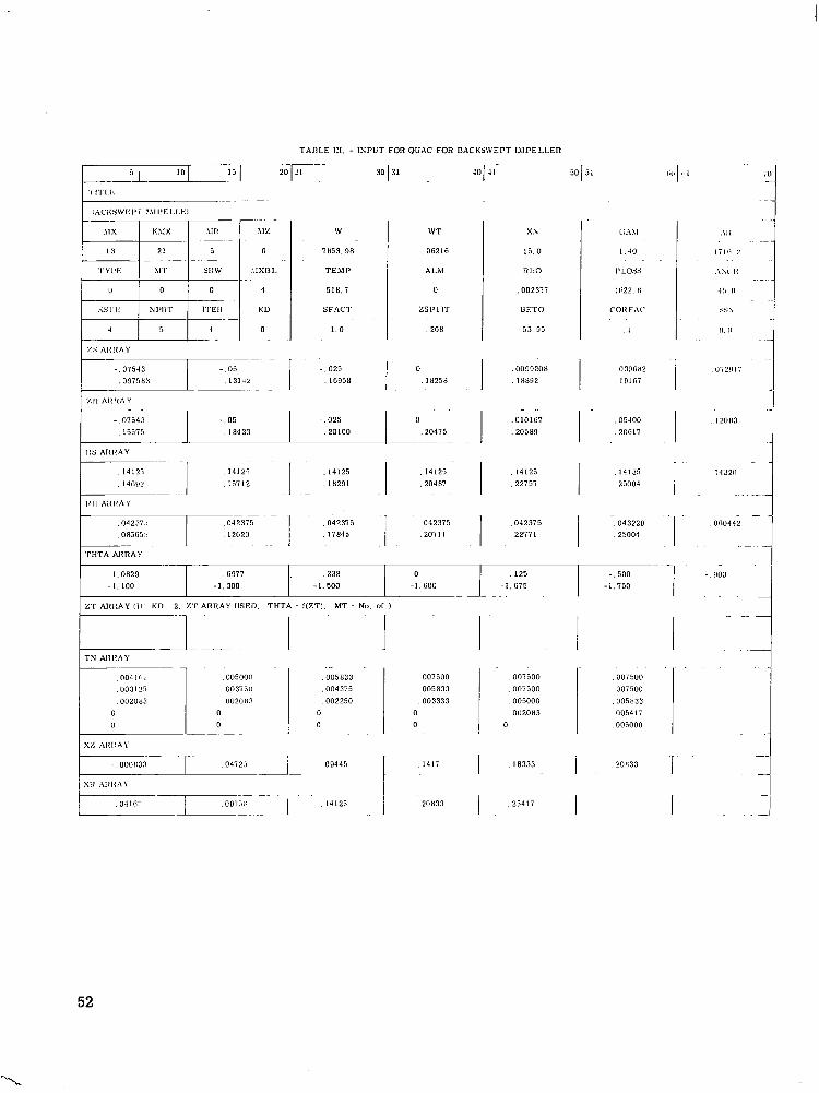
T A n L E 111. - IXPUT FOR Q U A C FOR DACKSWEI'T I.\IPELLER

G.411

1.40

I'LOSS

I1;22. H

COllFAC

I

0306H2

I01 (i7

,05400

. 20F17

25004

14135

. 25004 043229

\V

7853.88

TEA1 P

518. I

S F A C T

1.0

W T

. 06216

A LM

0

ZSPLIT

20 n

0

. ~ m n

0 .20475

x.\

I5 0

Rl lO

,002377

D E 7 0

-53 85

. 0 0 ~ 2 0 n

. I 8802

.OlOlG7 ,205~19

,14125 , 22757

,042315 22171

I I I I I I

I

, 14125 20487

. .

.042375

.207 I I

1 1

0 -I.G00 -1.675

-. 125 -1 .750 - , 500

. OOi500

OOiSOO ,005833

009000

0054 1 7

20H33

ZT ARRAY ( I 1 K D 2. Z T ARRAY USE]). THTA = I(ZT1. MT -- No. o f . )

T 1

1 .007500 . 0 0 7 5 0 0 005000 002083

0

. I 8333

. 2 5 4 1 7

,005833 "

,004375

.002250 0 0

007500 ,005833 .003333

0 0

. 1 4 1 i

20833

I- 09445

1 I4125

52

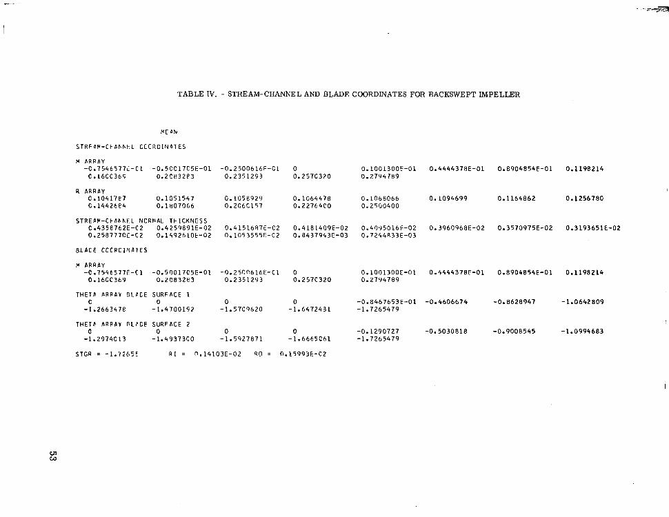
TABLE IV. - STREAM-CHANNEL AND BLADE COORDINATES FOR BACKSWEPT IMPELLER

N E AN

S T R F b P - C k b b h t L C C C R O I N A T E S

M D R R A Y -C.754t577i-C1 -0.50017C5E-01

C .16CC365 0.2CL!32P3

R A R R D Y c.10417e7 c.lwzte4

0.1G51547 0.1807066

S T R E b P - C l - 8 h h F L N C R M A L T H I C K N E S S C.43587t2E-C2 0.4259891E-02 0.258777CE-C2 0.1492610t-02

B L P C E C C C R C l N l l t S

C A R R b Y -C.754t577E-C1 -0.50017C5E-01 0.16CC369 0.2083283

T H E 1 8 A R R A Y O L b C E S U R F A C E 1 C 0

-1.2663478 -1.4700142

THETC P R P b Y P C C C E S U R F A C E 2 0 0 -1.29740 13 -1.49373CO

-0.2500616F-C1 0.2351293

0.1058929 0.2C6C157

0.4151687E-CZ 0.1053555E-C2

-0.250C616E-Cl 0.2351293

0 - 1.5709620

0 -1.5927871

0 0.2570370

0.1064478 0.227C4CO

0.4181409E-02 0.8437943E-03

0 0.2576320

0 -1.6472431

0 -1.6665C61

0.1001300E-01 0.2794789

0.1068066 0.2500400

0.4095016F-02 0.7244833E-03

0.1001300E-01 0.2794789

-0.8467653E-01 -1.7265479

-0.1270727 -1.7265479

0.4444378E-01

0.1094699

0.3960968E-02

0.4444378F-01

-0.4606674

-0.5030818

0.8904854E-01

0.1164862

0.3570975E-02

0.8904854E-01

-0.8628947

-0.9008545

0.1198214

0.1256780

0.3193651E-02

0.1198214

-1.0642809

-1.0994683

m w

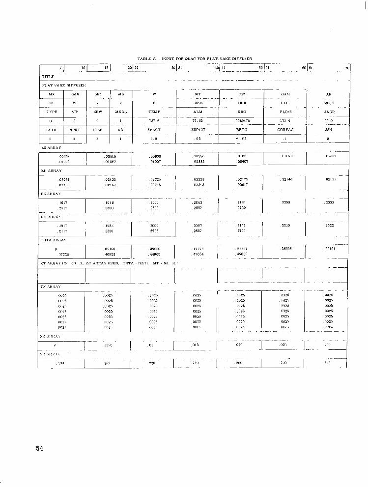
TABLE V. - INPUT FOR QUAC FOR FLAT-VANE DIFFUSER

- ~ . "" ~ ~ ~

_ ~- ~

,0089470

,00996 ,0105 ,01078 00882 .DO607

1711 A I I l t A Y

. 1917 1958

. 2 4 I i , 2500

TII'I'A A I t I t A Y

0 .051G6 3722n ,40823

" .

Z'l' A l O < A \ [ I F K i l 2. Z T r\RRAY USED. THTA - f (ZT) . MT .- No. uf. 1

0025 .0025 .(lo25 002s 0025

0025 002.)

" ."

.0025

.0025 002s 0025 0025 002s 0025

_

.002s 0025 002s 0025

.0025 0025 002s "

002s no25 0025

0025

0 0 2 i no25 11n2-)

~ " .~

12 i. At<

S T K E ~ t " C k ~ h h r . L CLCRUIrJfiTFS

P a H w m Y I: iJ.4 1 C r ) O C 15-02 C.5"3cC;Cl"C I 0.656c,f;CoF-lil

R A H R l l Y C.1417CCC; rj.175flrC:I C.25CCCl'C 0.2c;P:0co

STPEAP-CkPhhKL h C R t ' A L T P I C K ' J E S S CSS114576k-C3 C . T'i4odC3E-03 0.551!153:--C3 1).h>4t;')',HC-G3

HLACE CCLPCl l Ib lEs

P A R I I A Y C 0.41COOClF-02 C.583CCCCL-Cl O.hh6CCCOe-01

THETC b R P b Y tILCC€ SURFACE 1 C 0.5C948?8F-O1 C.39R7?S4 3.i 30746 1

THETP A R R I Y r4LCCE SURkPCE 2 0 C.3844C!I

0 .1S i5362E-01 0.4173164

TABLE VI. - STREAM-CHANNEL AND BLADE COORDINATES FOR DIFFUSER

o .2cocccc O.LG67CCO

C.fI3030COC-C2 0.75CCGOOE-C1

0.9419942E-Cl 0 .4601997

0.16hCC9OE-Ol 0.812CCOOE-01

O.2CR3C(30 C.272SCOO

0.166CCOOE-01 O.Bl2CCPOE-Ol

0.1432913 0.47C2807

0.250COOOE-01

0.2167000

0.5h28559E-03

0.25OCOOOC-01

0.2?74512

0.2069713

0.333OOOOF-01

0.2250COO

0.5343616E-03

0.3330000E-01

0.2785887

0.2602138

0.4160000E-01

0.2333000

0.5232948E-03

0.4160000E-01

0.3233202

0.3065823

0 . 5 0 0 0 0 G 0 ~ - 0 1

0.2417000

0.5265550E-03

0.5OOOOOOE-01

0.3633232

0.3479192

UI UI

T A D L E VII. - INPUT FOR QUAC FOR RADIAL IMPELLER ._

5 I U 1 -1 20 21 30 31 40 I 4 1 " GO (:I _ _ _ ~ -

T1.r LE in I I ~ A I N A I l M l ~ E l . L L l f

h.1 x tiAh1 xs WT W n u a11t KhIX

10

AXGIl 1'1 0 s RllO A L h l T E M P l l X l l L SllW hl l ' 'r Y 1'E

I 2 4 6 I 1. Iifii 1 5 . 0 .018915 4031.7 10 6 21

0

n I - 2 1 0 . 16 1 . 0 2 1 5 0

SSK COIlFAC nETO ZSPLIT S F A C T KD I l E l l KPIIT lis'I'II

4 5 . 0 1 6 4 . 0 ,001293 0 5 3 6 . 0 1 0 11 ~ _ _ ~ _ _

ZS ARllAY

0 .088916 ,0164 1 6 ,05975 .043083 ,02225 . 11 967 , 13317 13108

I O ~ H

X11 ARRAY

0 . 1106i . 10142 .016416 .051416 -02225 . 14642 . 15142

. I3642 . 15142

RS Al lRAY

. 14592

. 19161 . 17325 . I60fi7 . 14100 . 14G00 . 15415 . 14915

,2250 ,2490

RII ARRAY

,017416 l ing2

,0775 ,22283

,0805 ,2490

. o m 1 6 6 . 15033 ,12217 1035

THTA AIIItAY

0 -. 6120

-. 2659 - _ 1185 -. 5924

- .5519 - .4802 - . 018 -. 6120

-. 3145 -. 6069

ZT AIIRAY ( I F KD 2. ZT A R R A Y U S E D . T H l A = f (ZT) . MT 7 No. 01.)

0 . 15142 ,02225 ,013911 ,0055833

,08415 .I1433 .09125 ,03475 . Ofi8083 ,051416

TN ARRAY

,002667 .0125 0 0 2 0 ~ 3

-00125 .01083

oono 0 . 0

.00575

0.0 .00350

0 . 0 ,001 1G7

(Z ARRAY

,003411 ,0125 ,002500 ,01146 .001411 0 0 8 7 0 ~

0 . 0 ,00650

0 . 0

,00425 0 . 0

,001958

,00415

,003458 ,0125

,01146 .001833 .01012

0.0 .001833

0.0 ,005667

0 . 0 ,003208

,009083

,00675

.003792

.00141i

0 . 0

0 . 0

.01015

00825

, 0 0 5 I61

002708

0 . 0

0 . 0

.01167

.00025

-006208

,003192

,001375

0 0

,0125

.01017

007 I R 7

,004833

, 00250

0 . 0

- , 000R33 ,018083 .005583 12375 . 1331i

,05975 11433 . 10142 . OH3i5 , 15167

;If ARIIAY

,075 21867 18333 10833 1500 I

56 NASA-Langley, 1972 - 1 E- 6 592

' : I ' NATIONAL AERONAUTICS AND SPACE ADMISTRATION

WASHINGTON, D.C. 20546 POSTAGE AND FEES PAID

NATIONAL AERONAUTICS AND

SPACE ADMINISTRATION OFFICIAL BUSINESS FIRST CLASS MAIL,

PENALTY FOR PRIVATE USE $300 USMAIL

019 0 0 1 C 1 D 0 1 720204 S00903DS

AP WEAPONS LAB (AFSC) TECH LIBRARY/WLOL/ ATTN: E L O U BOWMAN, CHIEF KIETLAND AFB N M 87117

DEPT OF T H E a m FORCE

If Undeliverable (Section 1S8 Portal Manual) Do Not Rerur

' . ' b . 4 ~ . ... . ..

! -: . - . 9 . ,

"The aeronautical and space activities of the United States shall be conduited so as to contribute . . . to the expansion of human knowledge of phenomena i n the atnlosphere and space. The Adnzinistrcrtion shall provide for the widest pmcticable and appropriate dissemination of infdznlation concerning its activities and the results thereof."

.., ,

'. ' I -NATIONAL AERONAUTICS AND SPACE

. ,

NASA SCECNTIFIC .. > AND TECHNICAL

TECHNICAL R E P O k S : Scientific and technical information:considered important, complete, and a lasting contribution to existing knowledge. '.

TECHNICAL NOTES: Information less broad in scope but neveitheless of importance as a contribution to eikting knowledge.

TECHNICAL MEMORANDUMS: Information receiving limited distribution because of preliminary data, security classifica- tion, or other reasons.

ACT OF 1958

PUBLICATIONS

TECHNICAL TRANSLATIONS: Information published in a foreign language considered to merit NASA distribution in English.

SPECIAL PUBLICATIONS: Information derived from or of value to NASA activities. Publications include conference proceedings, monographs, data compilations, handbooks, sourcebooks, and special bibliographies.

TECHNOLOGY UTILIZATION PUBLICATIONS: Information on technology used by NASA that may be of particular

CONTRACTOR REPORTS: Scientific and technical information generated under a NASA Technology Utilization R~~~~~~ and contract or grant and considered an important contribution to existing knowledge.

interest in commercial and other non-aerospace npplications. Publications include Tech Briefs,

Technology Surveys.

Details on the availability of these publications may be obtained from:

SCIENTIFIC AND TECHNICAL INFORMATION OFFICE

NATIONAL AERONAUTICS AND SPACE ADMINISTRATION Wasbington, D.C. PO546

VELOCITIES IN THE MERIDIONAL PLANE OF A … PROGRAM FOR CALCULATING VELOCITIES IN THE MERIDIONAL...

Documents

Transcript of VELOCITIES IN THE MERIDIONAL PLANE OF A … PROGRAM FOR CALCULATING VELOCITIES IN THE MERIDIONAL...