Vehicle Tracking and Speed Estimation from Traffic Videos

Shuai Hua1, Manika Kapoor1, David C. Anastasiu1∗

1Department of Computer Engineering1San Jose State University, San Jose, CA

{shuai.hua, manika.kapoor, david.anastasiu}@sjsu.edu ∗

Abstract

The rapid recent advancements in the computation abil-

ity of everyday computers have made it possible to widely

apply deep learning methods to the analysis of traffic

surveillance videos. Traffic flow prediction, anomaly detec-

tion, vehicle re-identification, and vehicle tracking are basic

components in traffic analysis. Among these applications,

traffic flow prediction, or vehicle speed estimation, is one

of the most important research topics of recent years. Good

solutions to this problem could prevent traffic collisions and

help improve road planning by better estimating transit de-

mand. In the 2018 NVIDIA AI City Challenge, we combine

modern deep learning models with classic computer vision

approaches to propose an efficient way to predict vehicle

speed. In this paper, we introduce some state-of-the-art ap-

proaches in vehicle speed estimation, vehicle detection, and

object tracking, as well as our solution for Track 1 of the

Challenge.

1. Introduction

The continuously increasing number of on-road vehicles

has put a lot of pressure on road capacity and infrastruc-

ture, making traffic management difficult and giving way

to problems like congestion, collisions, and air pollution,

among others. These problems have significant impact on

our daily lives. A robust and efficient traffic management

system is required to reduce their effect. A large amount

of traffic data is generated daily. Traffic data contains in-

formation related to traffic flow, distribution, pattern, and

collisions, which can be used to solve various traffic related

issues. The volume and distribution of traffic can be used to

build appropriate structural and geometric designs for road

segments. Traffic collisions can be analyzed to see the cor-

relation of traffic volume and number and severity of colli-

sions, which in turn can help to investigate and assess col-

∗Corresponding author: David C. Anastasiu,

david.anastasiu at sjsu.edu.

lision risks. Apart from these problems related to vehicle

traffic, the data can also help in studies related to the reduc-

tion of environment pollution and fuel consumption. Also,

various statistical parameters, such as the average number

of vehicles on the road at a certain time, and the state of

congestion, can be studied, which can provide some infor-

mation for managing the highway [17].

To address these pressing issues, NVIDIA initiated a se-

ries of challenges aimed at the intersection of Artificial In-

telligence and Smart City. The first AI City Challenge, or-

ganized in 2017, focused on object detection, localization,

and classifications. The 2018 AI City Challenge continues

to promote deep learning and computer vision approaches

to help analyze urban traffic videos, and finally improve

traffic conditions and prevent traffic collisions. This work-

shop especially focuses on solving serious problems related

to urban traffic. Specifically, the challenge is comprised of

three tracks: Track1 (Traffic Flow Analysis) aims at devel-

oping models that can predict the driving speed of vehicles

in videos recorded by stationary cameras on highways or

at intersections. Track2 (Anomaly Detection) focuses on

detecting driving anomalies, such as stalled vehicles or car

accidents, in the videos. Track3 (Multi-camera Vehicle De-

tection and Re-identification) aims to detect and track all

vehicles in a set of videos which appear in each of a subset

of the videos recorded at different locations within the city.

In this paper, we propose a formulation to solve Track1.

Our model relies heavily on vehicle detection and track-

ing. In this Challenge, however, it is hard to train a vehi-

cle detection model from scratch since no labeled data is

provided. Instead, we leverage transfer learning and per-

form inference on our dataset using the 3D Deformable

model [16] for vehicle detection. As an alternative to the 3D

Deformable model, we considered the model by Bhandary

et al. [2], which obtained similar performance in the 2017

challenge. To be able to compare these two models on the

target reference data, we extract all frames from one of the

Track 1 videos and measure the models’ performance on

the frames, comparing the vehicle detection performance as

measured by mean Average Precision (mAP). The experi-

153

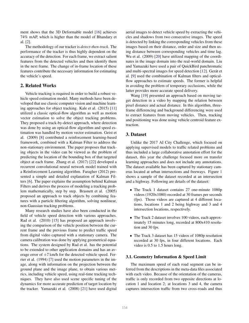
ment shows that the 3D Deformable model [16] achieves

74% mAP, which is higher than the model of Bhandary et

al. [2].

The methodology of our tracker is detect-then-track. The

performance of the tracker is thus highly dependent on the

accuracy of the detection. For each frame, we extract salient

features from the detected vehicles and then identify them

in the next frame. The change of in-frame location of these

features contribute the necessary information for estimating

the vehicle’s speed.

2. Related Works

Vehicle tracking is required in order to build a robust ve-

hicle speed estimation model. Many methods have been de-

veloped that use classic computer vision and machine learn-

ing approaches for object tracking. Kale et al. (2015) [11]

utilized a classic optical-flow algorithm as well as motion

vector estimation to solve the object tracking problems.

They proposed a track-by-detect approach, where detection

was done by using an optical-flow algorithm and speed es-

timation was handled by motion vector estimation. Geist et

al. (2009) [8] contributed a reinforcement learning-based

framework, combined with a Kalman Filter to address the

non-stationary environment. The paper proposes that track-

ing objects in the video can be viewed as the problem of

predicting the location of the bounding box of that targeted

object at each frame. Zhang et al. (2017) [22] developed a

recurrent convolutional neural network model trained with

a Reinforcement Learning algorithm. Faragher (2012) pre-

sented a simple and detailed explanation of Kalman Fil-

ters [6]. The paper explains the assumption behind Kalman

Filters and derives the process of modeling a tracking prob-

lem mathematically, step by step. Brasnett et al. (2005)

proposed an approach to track objects by combining fea-

tures with a particle filtering algorithm, solving nonlinear,

non-Gaussian tracking problems.

Many research studies have also been conducted in the

field of vehicle speed detection with various approaches.

Rad et al. (2010) [15] has proposed an approach involv-

ing the comparison of the vehicle position between the cur-

rent frame and the previous frame to predict traffic speed

from digital video captured with a stationary camera. The

camera calibration was done by applying geometrical equa-

tions. The system designed by Rad et al. has the potential

to be extended to other application domains and has an av-

erage error of ±7 km/h for the detected vehicle speed. Fer-

rier et al. (1994) [7] used the motion parameters in the im-

age, along with information on the projection between the

ground plane and the image plane, to obtain various met-

rics, including vehicle speed, using real-time tracking tech-

niques. They have also used scene specific tuning of the

dynamics for more accurate prediction of target location by

the tracker. Yamazaki et al. (2008) [21] have used digital

aerial images to detect vehicle speed by extracting the vehi-

cles and shadows from two consecutive images. The speed

is detected by linking the corresponding vehicles from these

images based on their distance, order and size and then us-

ing distance between corresponding vehicles and time lag.

Wu et al. (2009) [20] have utilized mapping of the coordi-

nates in the image domain into the real-world domain. Liu

and Yamazaki have used a pair of QuickBird panchromatic

and multi-spectral images for speed detection [12]. Gerat et

al. [9] used the combination of Kalman filters and optical-

flow approaches to estimate speeds. The former is helpful

in avoiding the problem of temporary occlusions, while the

latter provides more accurate speed delivery.

Wang [19] presented an approach based on moving tar-

get detection in a video by mapping the relation between

pixel distance and actual distance. In this algorithm, three-

frame differencing and background differencing were used

to extract features from moving vehicles. Then, tracking

and positioning was done using vehicle centroid feature ex-

traction.

3. Dataset

Unlike the 2017 AI City Challenge, which focused on

applying supervised models to traffic related problems and

thus included a large collaborative annotation effort for the

dataset, this year the challenge focused more on transfer

learning approaches and does not include any annotations.

The dataset available has been captured by stationary cam-

eras located at urban intersections and freeways. Figure 1

shows a sample of the dataset recorded at an intersection

and a highway. Following are details of the dataset:

• The Track 1 dataset contains 27 one-minute 1080p

videos (1920x1080) recorded at 30 frames per seconds

(fps). Those videos are captured at 4 different loca-

tions, locations 1 and 2 being highway and 3 and 4

intersection locations, respectively.

• The Track 2 dataset involves 100 videos, each approx-

imately 15 minutes long, recorded at 800x410 resolu-

tion and 30 fps.

• The Track 3 dataset has 15 videos of 1080p resolution

recorded at 30 fps, in four different locations. Each

video is 0.5 to 1.5 hours long.

3.1. Geometry Information & Speed Limit

The maximum speed of each road segment can be in-

ferred from the descriptions in the meta-data files associated

with each video. Because of the orientation of the cameras,

traffic is only recorded from two opposite directions at lo-

cation 1 and location 2; at locations 3 and 4, the camera

captures intersection traffic from two cross-roads and thus

154

Figure 1. A sample of images captured at traffic intersections and

highway.

Table 1. Geometry & speed limit data for track 1.

Loc. Latitude Longitude Direction Speed

1 37.316788 -121.950242 E → W 65 MPG

2 37.330574 -122.014273 NW → SE 65 MPG

3 37.326776 -121.965343 NW → SE 45 MPG

3 37.326776 -121.965343 NE → SW 35 MPG

4 37.323140 -121.950852 N → S 35 MPG

4 37.323140 -121.950852 E → W 35 MPG

Figure 2. VGG image annotation tool.

four different directions. Table 1 summarizes the location

and speed limit information for each video for track 1, for

one direction of each road. The opposite direction has the

same posted speed limit.

3.2. Annotation tool

We generated some ground-truth data to evaluate differ-

ent models for vehicle detection. The tool we used to anno-

tate data is the VGG Image Annotator(VIA) [5]. This tool

is browser-based and supports advanced functionality, such

as copy/paste of a bounding box. Since the frames we an-

notated are sequential and the position of vehicles changes

little from frame to frame, VGG is an easy tool to use to

label challenge data. Figure 2 shows a screen-shot of the

VGG tool.

4. Methodology

In this section, we introduce our methods for tracking

vehicles in traffic videos and estimating their speed. Our

method takes a detect-then-track approach and can use ob-

ject detections from any vehicle detection algorithm as in-

put. We will discuss, in turn, our strategy for ensuring

quality detections, identifying vehicle tracks, and estimat-

ing their speed.

4.1. Vehicle Detection

Given the fact that the 2018 AI City Challenge dataset

did not provide any ground-truth detection or tracking an-

notations, we were not able to train a vehicle detection

model specific to this dataset. Instead, we rely on trans-

fer learning, taking advantage of state-of-the-art deep learn-

ing models that have been previously trained for this task.

Specifically, the videos in Tracks 1 and 3 of the dataset

are similar in quality and scope to videos used for the ob-

ject detection, localization, and classification task of the

2017 AI City Challenge [14]. As such, we have cho-

sen to rely on the top-2 best performing models from that

challenge, the 3D Deformable model by Tang et al. [16]

and our lab’s submission to that challenge, the model by

Bhandary et al. [2]. Both models provide as output, for each

frame, a series of bounding-boxes believed to contain an ob-

ject of interest, the class of that object, and a confidence

score. The 2017 challenge sought to localize and clas-

sify objects in 14 categories, including car, suv, smalltruck,

mediumtruck, largetruck, pedestrian, bus, van, groupofpeo-

ple, bicycle, motorcycle, trafficsignal-green, trafficsignal-

yellow, and trafficsignal-red. In order to maximize the util-

ity of the detections we will provide as input to our algo-

rithm, we filter the detector output as follows:

• Remove detections with a confidence less than some

threshold α.

• Remove detections for non-vehicle classes, keeping

only those for the car, suv, smalltruck, mediumtruck,

largetruck, bus, van, bicycle, and motorcycle classes.

• Filter bounding boxes within the same frame that have

an overlap, measured by the Intersection-over-Union

(IOU) score, of at least some threshold β. Detections

are filtered while traversing the frame in a left-right

top-down order when the IOU of the detection with an

already selected bounding box is greater than β.

4.2. Vehicle Tracking

Our vehicle tracking algorithm relies on localization re-

sults from the vehicle detection methods described in Sec-

tion 4.1, which are enhanced with optical-flow based fea-

tures to provide robust vehicle trajectories.

4.2.1 Tracking-by-Detection

Given the fact that the input footage was at 1080p resolu-

tion and 30 fps, objects move few pixels from one frame

155

to the next. We thus define an efficient algorithm to define

initial object tracks based solely on the overlap of detected

object bounding boxes in consecutive frames. Specifically,

for each object in a frame, in decreasing order of detection

confidence, we assign the ID of the not already assigned ob-

ject with the highest IOU score in the previous h frames, as

long as that score is above a minimum threshold i.

Tracking-by-detection works well in practice for our set-

ting, but is prone to a high rate of ID changes when the

detector fails to localize an object for more than h frames.

Moreover, detectors often provide loose localization bound-

ing boxes around the detected objects, which shift several

pixels around the object from frame to frame, making speed

estimation from bounding boxes inaccurate. Figure 3 shows

a couple examples of detection errors, including a tree and

buildings being detected as vehicles and wide margins be-

tween the bounding-box and the detected object in some

cases.

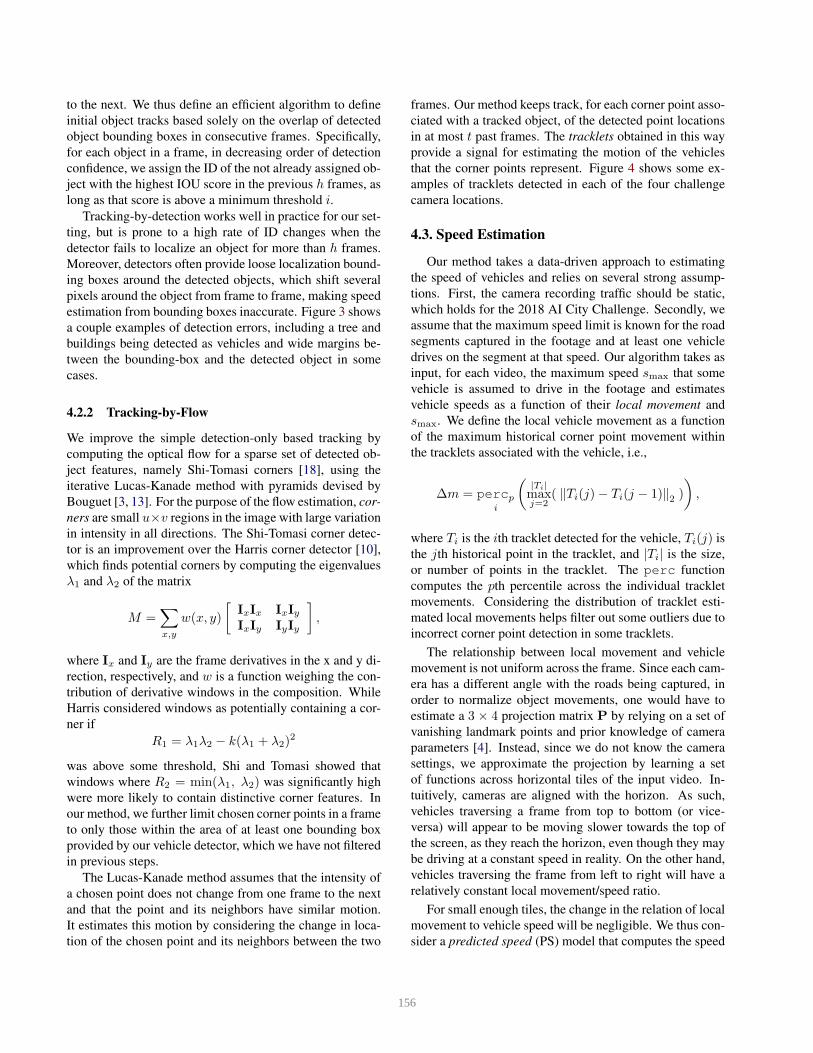
4.2.2 Tracking-by-Flow

We improve the simple detection-only based tracking by

computing the optical flow for a sparse set of detected ob-

ject features, namely Shi-Tomasi corners [18], using the

iterative Lucas-Kanade method with pyramids devised by

Bouguet [3, 13]. For the purpose of the flow estimation, cor-

ners are small u×v regions in the image with large variation

in intensity in all directions. The Shi-Tomasi corner detec-

tor is an improvement over the Harris corner detector [10],

which finds potential corners by computing the eigenvalues

λ1 and λ2 of the matrix

M =∑

x,y

w(x, y)

[

IxIx IxIy

IxIy IyIy

]

,

where Ix and Iy are the frame derivatives in the x and y di-

rection, respectively, and w is a function weighing the con-

tribution of derivative windows in the composition. While

Harris considered windows as potentially containing a cor-

ner if

R1 = λ1λ2 − k(λ1 + λ2)2

was above some threshold, Shi and Tomasi showed that

windows where R2 = min(λ1, λ2) was significantly high

were more likely to contain distinctive corner features. In

our method, we further limit chosen corner points in a frame

to only those within the area of at least one bounding box

provided by our vehicle detector, which we have not filtered

in previous steps.

The Lucas-Kanade method assumes that the intensity of

a chosen point does not change from one frame to the next

and that the point and its neighbors have similar motion.

It estimates this motion by considering the change in loca-

tion of the chosen point and its neighbors between the two

frames. Our method keeps track, for each corner point asso-

ciated with a tracked object, of the detected point locations

in at most t past frames. The tracklets obtained in this way

provide a signal for estimating the motion of the vehicles

that the corner points represent. Figure 4 shows some ex-

amples of tracklets detected in each of the four challenge

camera locations.

4.3. Speed Estimation

Our method takes a data-driven approach to estimating

the speed of vehicles and relies on several strong assump-

tions. First, the camera recording traffic should be static,

which holds for the 2018 AI City Challenge. Secondly, we

assume that the maximum speed limit is known for the road

segments captured in the footage and at least one vehicle

drives on the segment at that speed. Our algorithm takes as

input, for each video, the maximum speed smax that some

vehicle is assumed to drive in the footage and estimates

vehicle speeds as a function of their local movement and

smax. We define the local vehicle movement as a function

of the maximum historical corner point movement within

the tracklets associated with the vehicle, i.e.,

∆m = percpi

(

|Ti|maxj=2

( ‖Ti(j)− Ti(j − 1)‖2)

)

,

where Ti is the ith tracklet detected for the vehicle, Ti(j) is

the jth historical point in the tracklet, and |Ti| is the size,

or number of points in the tracklet. The perc function

computes the pth percentile across the individual tracklet

movements. Considering the distribution of tracklet esti-

mated local movements helps filter out some outliers due to

incorrect corner point detection in some tracklets.

The relationship between local movement and vehicle

movement is not uniform across the frame. Since each cam-

era has a different angle with the roads being captured, in

order to normalize object movements, one would have to

estimate a 3 × 4 projection matrix P by relying on a set of

vanishing landmark points and prior knowledge of camera

parameters [4]. Instead, since we do not know the camera

settings, we approximate the projection by learning a set

of functions across horizontal tiles of the input video. In-

tuitively, cameras are aligned with the horizon. As such,

vehicles traversing a frame from top to bottom (or vice-

versa) will appear to be moving slower towards the top of

the screen, as they reach the horizon, even though they may

be driving at a constant speed in reality. On the other hand,

vehicles traversing the frame from left to right will have a

relatively constant local movement/speed ratio.

For small enough tiles, the change in the relation of local

movement to vehicle speed will be negligible. We thus con-

sider a predicted speed (PS) model that computes the speed

156

Figure 3. Detection error. (Best viewed in color)

Loc 1 Loc 2

Loc 3 Loc 4

Figure 4. Tracklets obtained through optical-flow estimation. (Best viewed in color)

of a vehicle, in each tile, as

s =∆m

maxT

∆m× smax,

where maxT

∆m is the maximum local movement in any

tracklet of a vehicle passing through the tile within a win-

dow ∆t of the current vehicle. We further smooth out out-

liers by considering the maximum estimated vehicle speed

over at most h past frames. Finally, we limit estimated

speeds within the range [0, smax].

Many of the cars drive at constant speeds through the

frame, especially in highway traffic without congestion, as

found in Loc 1 and 2 videos of the challenge. We thus con-

sider a second constant speed (CS) model, which assigns

the input smax speed to all detected vehicles in the video,

after first filtering based on confidence and track overlap.

5. Experiments

In order to choose one of the two detection models we

first considered in Section 4.1, we first manually labeled

the first 250 frames in video 1 of location 1 as our ground-

157

Table 2. Detection performance.

Mddel mAP 0 mAP 1

Bhandary [2] 0.34 0.34

3D Deformable Model [16] 0.28 0.74

truth, used both models to detect vehicles in the video, and

then compared the mean Average Precision (mAP) of the

two models. For each model, we filtered low-confidence

detections with confidence scores α below 0.0 (no filter-

ing) and 0.1, respectively, which we denote in Table 2 by

mAP 0 and mAP 1. The results seem to indicate that the

3D Deformable model is superior to the one by Bhandary

et al., given proper confidence thresholding. In our Chal-

lenge submissions we tested 3D Deformable models with

minimum confidence scores α between 0.01 and 0.05.

All experiments were executed on a system equipped

with a 5th generation Core i7 2.8 GHz CPU, 16 GB RAM,

and an NVIDIA Titan X GPGPU. For each location, we

tested maximum speed limits smax±{5, 10, 15} miles/hour,

given posted speed limits noted in Table 1. For duplicate

detection filtering, we used an IOU threshold β of 0.9, Dur-

ing tracklet identification, we considered overlapping detec-

tions with minimum IOU 0.7, kept a history of up to h = 10corner points for each tracklet, and estimated local move-

ment from the top p = 80% tracklet segments.

The 2018 AI City Challenge Track 1 was evaluated based

on a composite score, S1 = DR× (1−NRMSE), where

DR is the vehicle detection rate for the set of ground-truth

vehicles, and NRMSE is the RMSE score across all de-

tections of the ground-truth vehicles, normalized via min-

max normalization with regards to the RMSE scores of all

best solutions of other teams submitting solutions to Track

1. Ground-truth vehicles were driven by NVIDIA employ-

ees through the camera viewpoints while recording instan-

taneous speeds with the aid of a GPS device. Additional

details regarding the Challenge datasets and evaluation cri-

teria can be found at [1].

6. Results

In this section, we analyze the results obtained by apply-

ing our tracking and speed estimation models to the Track 1

videos from the 2018 NVIDIA AI City Challenge. We first

describe our Challenge result and then analyze potential av-

enues of improvement for our model.

6.1. Challenge Submission

Our team’s best Challenge submission, which had a DR

score of 1.0 and an RMSE score of 12.1094, earned an S1score of 0.6547, 0.0017 below the next higher ranked team.

While our model had perfect detection performance, the

speed estimation component of our method was not accu-

rate enough to be competitive against the top teams, team48

and team79, which earned S1 scores of 1.0 and 0.9162, re-

spectively. Given the score of 1.0, it is clear that team48

also had a detection rate score of 1.0 and at the same time

managed the lowest RMSE score among the teams.

6.2. Model Analysis

Our best performing model was a constant speed model

with maximum speeds of 70, 70, 50, and 30, respectively,

for locations 1–4. Our predictive speed models suffered

from both lower detection rate and higher RMSE scores

than the CS model. Figure 5 shows the predicted speeds for

two consecutive frames from Location 1 using the PS (a)

and CS (b) models executed with the same parameters. The

PS model relies on the optical-flow-based tracklet detection

to estimate vehicle speeds and will only output a detection

if its speed can be reliably estimated. As such, a number of

vehicles that are detected in the CS model are missing from

the PS model output.

As a way to better understand the limitations of the PS

model, we selected 10 random tracks from each location

with a minimum length of 45 and maximum length of 60

frames, which we plot in Figure 7. While some tracks

show expected smooth transitions indicative of normal traf-

fic, many display sudden spikes in speed, which seems to

indicate the corner feature detector may be choosing alter-

nate similar corners in some frames.

We further verify the variability in speed estimates in the

PS model by plotting the distributions of speed ranges (dif-

ference between maximum and minimum speed) in tracks

of videos in all four locations. Given that most vehicles

are only seen for a few seconds while they pass through the

frame, they are expected to have almost constant speed and

very low variability. Each quadrant of Figure 6 shows, using

a line for each video at a given location, a uniform random

sample from the speed range distribution in the given video.

While some variability is expected due to normal traffic, our

model shows excessive variability, with almost 20% of vehi-

cles reporting more than 15 miles/hour variability. The per-

formance is even worse in Location 3, where videos capture

quality was impaired by constant camera movement due to

wind or bridge vibrations.

7. Conclusion & Future Work

In this paper, we introduced a model for tracking vehi-

cles in traffic videos based on a detect-then-track paradigm,

coupled with an optical-flow-based data-driven speed esti-

mation approach, and described our solutions for Track 1 of

the 2018 NVIDIA AI City Challenge. Our model performed

well but was not as competitive as some of the other Chal-

lenge teams, displaying excessive variability. Due to lack of

time, we did not compare our method against other detect-

then-track algorithms, which we leave as future work. Ad-

158

(a) Predicted Speed Model

(b) Constant Speed ModelFigure 5. Speed estimates of the predicted (a) and constant (b) speed models. (Best viewed in color)

0

20

40

60

Loc 1 Loc 2

0 20 40 60 80 1000

20

40

Loc 3

0 20 40 60 80 100

Loc 4 spee

d

Figure 6. Speed range distribution.

ditionally, we plan to investigate smoothing techniques for

the predicted vehicle speeds which may lead to improved

model performance.

References

[1] Data and Evaluation nvidia ai city challenge. https:

//www.aicitychallenge.org/?page_id=9. Ac-

cessed: 2018-04-01.

0

20

40

60Loc 1

0

20

40

60

Loc 2

0 20 40 600

10

20

30

40Loc 3

0 20 40 600

10

20

Loc 4

spee

d

track frameFigure 7. Speed of random tracks.

[2] N. Bhandary, C. MacKay, A. Richards, J. Tong, and D. C.

Anastasiu. Robust classification of city roadway objects for

traffic related applications. 2017.

[3] J.-Y. Bouguet. Pyramidal implementation of the lucas

kanade feature tracker description of the algorithm, 2000.

[4] B. Caprile and V. Torre. Using vanishing points for camera

calibration. Int. J. Comput. Vision, 4(2):127–140, May 1990.

[5] A. Dutta, A. Gupta, and A. Zissermann. VGG image anno-

159

tator (VIA). http://www.robots.ox.ac.uk/ vgg/software/via/,

2016. Accessed: January 10, 2018.

[6] R. Faragher. Understanding the basis of the kalman filter via

a simple and intuitive derivation [lecture notes]. IEEE Signal

Processing Magazine, 29(5):128–132, Sept 2012.

[7] N. J. Ferrier, S. Rowe, and A. Blake. Real-time traffic moni-

toring. In Proceedings of 1994 IEEE Workshop on Applica-

tions of Computer Vision, pages 81–88, 1994.

[8] M. Geist, O. Pietquin, and G. Fricout. Tracking in reinforce-

ment learning. In International Conference on Neural Infor-

mation Processing, pages 502–511. Springer, 2009.

[9] J. Gerat, D. Sopiak, M. Oravec, and J. Pavlovicova. Vehicle

speed detection from camera stream using image processing

methods. In ELMAR, 2017 International Symposium, pages

201–204. IEEE, 2017.

[10] C. Harris and M. Stephens. A combined corner and edge

detector. In Proceedings of the 4th Alvey Vision Conference,

pages 147–151, 1988.

[11] K. Kale, S. Pawar, and P. Dhulekar. Moving object

tracking using optical flow and motion vector estima-

tion. In Reliability, Infocom Technologies and Optimization

(ICRITO)(Trends and Future Directions), 2015 4th Interna-

tional Conference on, pages 1–6. IEEE, 2015.

[12] W. Liu and F. Yamazaki. Speed detection of moving vehi-

cles from one scene of quickbird images. In Urban Remote

Sensing Event, 2009 Joint, pages 1–6. IEEE, 2009.

[13] B. D. Lucas and T. Kanade. An iterative image registra-

tion technique with an application to stereo vision (darpa).

In Proceedings of the 1981 DARPA Image Understanding

Workshop, pages 121–130, April 1981.

[14] M. Naphade, D. C. Anastasiu, A. Sharma, V. Jagrlamudi,

H. Jeon, K. Liu, M. C. Chang, S. Lyu, and Z. Gao. The nvidia

ai city challenge. In 2017 IEEE SmartWorld Conference,

SmartWorld’17, Piscataway, NJ, USA, 2017. IEEE.

[15] A. G. Rad, A. Dehghani, and M. R. Karim. Vehicle speed

detection in video image sequences using cvs method. In-

ternational Journal of Physical Sciences, 5(17):2555–2563,

2010.

[16] Z. Tang, G. Wang, T. Liu, Y. Lee, A. Jahn, X. Liu, X. He,

and J. Hwang. Multiple-kernel based vehicle tracking using

3d deformable model and camera self-calibration. CoRR,

abs/1708.06831, 2017.

[17] P. H. Tobing et al. Application of system monitoring and

analysis of vehicle traffic on toll road. In Telecommunication

Systems Services and Applications (TSSA), 2014 8th Inter-

national Conference on, pages 1–5. IEEE, 2014.

[18] C. Tomasi and J. Shi. Good features to track. In Proc.

IEEE Conf. on Comp. Vision and Patt. Recog., pages 593–

600, 1994.

[19] J.-x. Wang. Research of vehicle speed detection algorithm

in video surveillance. In Audio, Language and Image Pro-

cessing (ICALIP), 2016 International Conference on, pages

349–352. IEEE, 2016.

[20] J. Wu, Z. Liu, J. Li, C. Gu, M. Si, and F. Tan. An algorithm

for automatic vehicle speed detection using video camera. In

Computer Science & Education, 2009. ICCSE’09. 4th Inter-

national Conference on, pages 193–196. IEEE, 2009.

[21] F. Yamazaki, W. Liu, and T. T. Vu. Vehicle extraction and

speed detection from digital aerial images. In Geoscience

and Remote Sensing Symposium, 2008. IGARSS 2008. IEEE

International, volume 3, pages III–1334. IEEE, 2008.

[22] D. Zhang, H. Maei, X. Wang, and Y.-F. Wang. Deep rein-

forcement learning for visual object tracking in videos. arXiv

preprint arXiv:1701.08936, 2017.

160